Cool DZ white dwarfs in the SDSSwhite dwarf. In the (u −g)vs. ( r) color-colordiagram,this star 1...
11
arXiv:1105.0268v1 [astro-ph.SR] 2 May 2011 Astronomy & Astrophysics manuscript no. 16816 c ESO 2018 August 29, 2018 Cool DZ white dwarfs in the SDSS D. Koester 1 , J. Girven 2 , B.T. G¨ ansicke 2 , and P. Dufour 3 1 Institut f¨ ur Theoretische Physik und Astrophysik, University of Kiel, D-24098 Kiel, Germany e-mail: [email protected] 2 Department of Physics, University of Warwick, Coventry, UK 3 D´ epartement de Physique, Universit´ e de Montr´ eal, Montr´ eal, QC H3C 3J7, Canada ABSTRACT Aims. We report the identification of 26 cool DZ white dwarfs that lie across and below the main sequence in the Sloan Digital Sky Survey (SDSS) (u − g) vs. (g − r) two-color diagram; 21 of these stars are new discoveries. Methods. The sample was identified by visual inspection of all spectra of objects that fall below the main sequence in the two-color diagram, as well as by an automated search for characteristic spectral features over a large area in color space that included the main sequence. The spectra and photometry provided by the SDSS project are interpreted with model atmospheres, including all relevant metals. Effective temperatures and element abundances are determined, while the surface gravity has to be assumed and was fixed at the canonical value of log g = 8. Results. These stars represent the extension of the well-known DZ sequence towards cooler temperatures and fill the gap around T eff = 6500 K present in a previous study. The metal abundances are similar to those in the hotter DZ, but the lowest abundances are missing, probably because of our selection procedures. The interpretation is complicated in terms of the accretion/diffusion scenario, because we do not know if accretion is still occurring or has ended long ago. Independent of that uncertainty, the masses of the metals currently present in the convection zones – and thus an absolute lower limit of the total accreted masses – of these stars are similar to the largest asteroids in our solar system. Key words. white dwarfs – stars: abundances – accretion – diffusion – line: profiles 1. Introduction Cool white dwarfs with traces of metals other than carbon are designated with the letter “Z” in the current classification sys- tem. If Balmer lines are visible, they are called DAZ or DZA, depending on whether hydrogen lines or some metal lines are the strongest. Helium-dominated DBs with metals are DBZ, and finally, at lower temperature where no hydrogen or helium lines remain visible, there are the DZs. Helium-rich DBZs and DZs have been known for a long time; in fact, one of the first three classical white dwarfs, van Maanen 2, belongs to this class (Kuiper 1941). DAZs were discovered much later (Koester et al. 1997; Holberg et al. 1997), but this is purely observational bias, since the metal line strengths are much weaker in hydrogen at- mospheres with lower transparency. The almost mono-elemental composition of the outer lay- ers is caused by gravitational settling, with time scales much shorter than the white dwarf evolutionary time scales. The met- als can therefore not be primordial. For decades the standard explanation has been accretion from interstellar matter (ISM), with subsequent diffusion downward out of the atmosphere. This scenario has been discussed in detail and compared with obser- vations in a series of three fundamental papers by Dupuis et al. (1992, 1993a,b). A special case is the DQ spectral class, with pollution by the element carbon. The carbon can be dredged- up from below the outer helium layer by a deepening con- vection zone and does not necessarily need an exterior source (Koester et al. 1982; Pelletier et al. 1986). The ISM accretion hypothesis for the DZ has a number of problems, the most disconcerting ones being the lack of dense Send offprint requests to: D. Koester interstellar clouds in the solar neighborhood, and in many cases a large deficit of hydrogen in the accreted matter. These argu- ments have been summarized by Farihi et al. (2010a), who in the same paper argue for the accretion of circumstellar dust as the source of the accreted matter. This dust is thought to orig- inate from the the tidal disruption of some rocky material, left over from a former planetary system (Debes & Sigurdsson 2002; Jura 2003). This idea has gained more and more acceptance in the last decade, mainly through the discovery of infrared ex- cesses due to circumstellar dust in a significant fraction of DAZs and DBZs (Jura 2006; von Hippel et al. 2007; Farihi et al. 2009, 2010b,a). In particular the gaseous disks with Ca ii emission lines (G¨ ansicke et al. 2006, 2007, 2008) are the strongest con- firmation for the disk geometry and its location inside the Roche lobe of the white dwarfs, a key prediction of the tidal disruption hypothesis. A sample of 147 cool He-rich metal polluted white dwarfs (spectral class DZ) identified by SDSS has been analyzed by Dufour et al. (2007). Of these, only two have T eff below 6600 K (at 6090 and 4660 K). Given that already about half a dozen cool DZ known within 20 pc of the Sun are brighter than this SDSS sample (including van Maanen 2 at only 4.3 pc, Sion et al. 2009) this suggests that a large number of cooler DZ remain to be found. 2. Color selection We have been investigating the spectroscopic data base for white dwarfs with unusual properties (G¨ ansicke et al. 2010), and iden- tified SDSS0916+2540 (which we adopt as notation for SDSS objects throughout this paper) as a cool, very metal-rich DZ white dwarf. In the (u −g) vs. (g −r) color-color diagram, this star 1
Transcript of Cool DZ white dwarfs in the SDSSwhite dwarf. In the (u −g)vs. ( r) color-colordiagram,this star 1...

arX
iv:1
105.
0268
v1 [
astr
o-ph
.SR
] 2
May
201
1Astronomy & Astrophysicsmanuscript no. 16816 c© ESO 2018August 29, 2018
Cool DZ white dwarfs in the SDSSD. Koester1, J. Girven2, B.T. Gansicke2, and P. Dufour3
1 Institut fur Theoretische Physik und Astrophysik, University of Kiel, D-24098 Kiel, Germanye-mail:[email protected]
2 Department of Physics, University of Warwick, Coventry, UK3 Departement de Physique, Universite de Montreal, Montreal, QC H3C 3J7, Canada
ABSTRACT
Aims. We report the identification of 26 cool DZ white dwarfs that lie across and below the main sequence in the Sloan Digital SkySurvey (SDSS) (u− g) vs. (g− r) two-color diagram; 21 of these stars are new discoveries.Methods. The sample was identified by visual inspection of all spectraof objects that fall below the main sequence in the two-colordiagram, as well as by an automated search for characteristic spectral features over a large area in color space that included the mainsequence. The spectra and photometry provided by the SDSS project are interpreted with model atmospheres, including all relevantmetals. Effective temperatures and element abundances are determined, while the surface gravity has to be assumed and was fixed atthe canonical value of logg = 8.Results. These stars represent the extension of the well-known DZ sequence towards cooler temperatures and fill the gap aroundTeff
= 6500 K present in a previous study. The metal abundances are similar to those in the hotter DZ, but the lowest abundances aremissing, probably because of our selection procedures. Theinterpretation is complicated in terms of the accretion/diffusion scenario,because we do not know if accretion is still occurring or has ended long ago. Independent of that uncertainty, the masses of the metalscurrently present in the convection zones – and thus an absolute lower limit of the total accreted masses – of these stars are similar tothe largest asteroids in our solar system.
Key words. white dwarfs – stars: abundances – accretion – diffusion – line: profiles
1. Introduction
Cool white dwarfs with traces of metals other than carbon aredesignated with the letter “Z” in the current classificationsys-tem. If Balmer lines are visible, they are called DAZ or DZA,depending on whether hydrogen lines or some metal lines arethe strongest. Helium-dominated DBs with metals are DBZ,and finally, at lower temperature where no hydrogen or heliumlines remain visible, there are the DZs. Helium-rich DBZs andDZs have been known for a long time; in fact, one of the firstthree classical white dwarfs, van Maanen 2, belongs to this class(Kuiper 1941). DAZs were discovered much later (Koester et al.1997; Holberg et al. 1997), but this is purely observationalbias,since the metal line strengths are much weaker in hydrogen at-mospheres with lower transparency.
The almost mono-elemental composition of the outer lay-ers is caused by gravitational settling, with time scales muchshorter than the white dwarf evolutionary time scales. The met-als can therefore not be primordial. For decades the standardexplanation has been accretion from interstellar matter (ISM),with subsequent diffusion downward out of the atmosphere. Thisscenario has been discussed in detail and compared with obser-vations in a series of three fundamental papers by Dupuis et al.(1992, 1993a,b). A special case is the DQ spectral class, withpollution by the element carbon. The carbon can be dredged-up from below the outer helium layer by a deepening con-vection zone and does not necessarily need an exterior source(Koester et al. 1982; Pelletier et al. 1986).
The ISM accretion hypothesis for the DZ has a number ofproblems, the most disconcerting ones being the lack of dense
Send offprint requests to: D. Koester
interstellar clouds in the solar neighborhood, and in many casesa large deficit of hydrogen in the accreted matter. These argu-ments have been summarized by Farihi et al. (2010a), who inthe same paper argue for the accretion of circumstellar dustasthe source of the accreted matter. This dust is thought to orig-inate from the the tidal disruption of some rocky material, leftover from a former planetary system (Debes & Sigurdsson 2002;Jura 2003). This idea has gained more and more acceptance inthe last decade, mainly through the discovery of infrared ex-cesses due to circumstellar dust in a significant fraction ofDAZsand DBZs (Jura 2006; von Hippel et al. 2007; Farihi et al. 2009,2010b,a). In particular the gaseous disks with Caii emissionlines (Gansicke et al. 2006, 2007, 2008) are the strongest con-firmation for the disk geometry and its location inside the Rochelobe of the white dwarfs, a key prediction of the tidal disruptionhypothesis.
A sample of 147 cool He-rich metal polluted white dwarfs(spectral class DZ) identified by SDSS has been analyzed byDufour et al. (2007). Of these, only two haveTeff below 6600 K(at 6090 and 4660 K). Given that already about half a dozencool DZ known within 20 pc of the Sun are brighter than thisSDSS sample (including van Maanen 2 at only 4.3 pc, Sion et al.2009) this suggests that a large number of cooler DZ remain tobe found.
2. Color selection
We have been investigating the spectroscopic data base for whitedwarfs with unusual properties (Gansicke et al. 2010), andiden-tified SDSS0916+2540 (which we adopt as notation for SDSSobjects throughout this paper) as a cool, very metal-rich DZwhite dwarf. In the (u−g) vs. (g−r) color-color diagram, this star
1

D. Koester et al.: Cool DZ white dwarfs in the SDSS
Fig. 1. SDSS Two-color diagram for objects with spectra iden-tified as normal stars (grey S-shaped region in the middle ofthe figure), QSO (cyan dots), DZ white dwarfs analyzed byDufour et al. (2007) (solid black dots) and cool “extreme” DZdiscovered by our search (red open circles).
lies below the main sequence, a region that has hitherto not beensystematically explored for its stellar content. SDSS intensivelytargeted this region as part of its quasar program (Richardset al.2002). Inspecting all spectroscopic objects within SDSS DataRelease 7 (Abazajian et al. 2009) that have colors within thedashed region shown in Fig. 1 confirms that the vast majorityarez ∼ 3 quasars, however, we also identified 16 of these ob-jects as cool DZ white dwarfs characterized by a strong com-plex of MgI absorption lines near 5170 Å (one of these turnedout to be a carbon-rich DQ, see below). This finding, coupledwith the fact that all except one of the SDSS DZ stars analyzedby Dufour et al. (2007) are located above the main sequence in(u− g) vs. (g− r) (Fig. 1) strongly suggested that part of the DZpopulation will fall right into the color space occupied by themain sequence. In the view of the large number of DR7 spec-tra of ∼K-A type stars we developed a search routine in theregion bounded by the solid lines in Fig. 1, which checks forthe characteristic spectral features, foremost the Mgi lines near5170 Å. Secondary criteria were the presence of the Na D linesand the absence of Hα. A heavy contamination are still K starswith molecular bands of MgH, but since the slope of the spec-trum is quite different, they can be identified by visual inspec-tion. This procedure led to the discovery of nine additionalDZwhite dwarfs, two of which were already in the Dufour sample.Two additional objects, SDSS0143+0113 and SDSS2340+0817,were identified independently by Dufour in a search for DZs.The complete list of cool DZ (plus one DQ) white dwarfs iden-tified and theirugrizphotometry is given in Table 1.
3. Input physics and models
3.1. Line identification and broadening
All spectral features found in the spectra of the new coolDZ white dwarfs can be identified with lines from Ca, Mg,
3900.0 3920.0 3940.0 3960.0
3.00
4.00
5.00
6.00
7.00
8.00
9.00
λ [Α]
log
P(λ)
3500.0 4000.0 4500.0
-2.50
0.00
2.50
5.00
7.50
λ [Α]
log
P(λ)
Fig. 2. Quasi-static line profile for the CaiiK resonance line(dashed, red), compared with the impact approximation (con-tinuous, black). Parameters are 6000 K for the temperature anda neutral He perturber density of 1019cm−3. The central regionis enlarged in the top panel. The quasi-static calculation is onlyuseful for the wing; approximately within the central region be-tween the crossing points of the two profiles the impact calcula-tion is the superior approximation.
Na, Fe, Ti, and Cr, broadened predominantly through vander Waals broadening by neutral helium. The broadest linesshow strongly asymmetric profiles, which were in the caseof Mg i 5169/5174/5185 originally identified as due to quasi-static broadening by Wehrse & Liebert (1980) in their study ofSDSS1330+3029 (=G165-7). The same conclusion was reachedby Kawka et al. (2004) for SDSS1535+1247; both of these starsare in our present sample. The width of these lines, as well asthat of the Caii resonance lines is far beyond the range of valid-ity of the impact approximation, which is in these cases approxi-mately 8-10 Å from the line centers (see p. 312 in Unsold 1968).We have used the simple and elegant method of Walkup et al.(1984), who present numerical calculations for the transitionrange between impact and quasi-static regime, which can in bothlimits be easily extended with the asymptotic formulae. Theseprofiles are reasonable approximations for the MgI triplet.
For the much wider Caii resonance lines this approximationfails. The reason is very likely that for such strong interactionsneeded to produce a 600 Å wide wing the approximation witha simple van der Waalsr−6 law is not valid. We have used thequasi-static limit of the semiclassical quasi-molecular broaden-ing theory as described in Allard & Kielkopf (1982). This for-mulation (e.g. their eq. 59 in the cited paper) easily allowstheincorporation of a Boltzmann factor to account for the variationof the perturbation probability with distance of the perturber inthermal equilibrium. It would also allow us to take a variationin the dipole moments into account, which, however, are appar-ently not available in the published literature.
2
D. Koester et al.: Cool DZ white dwarfs in the SDSS
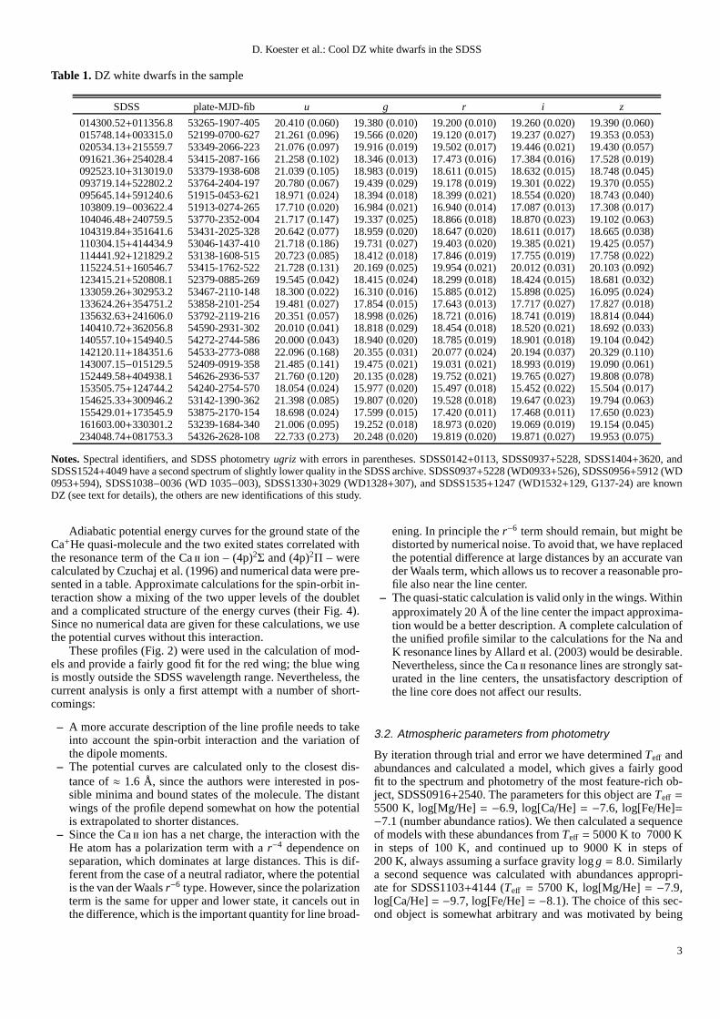
Table 1.DZ white dwarfs in the sample
SDSS plate-MJD-fib u g r i z
014300.52+011356.8 53265-1907-405 20.410 (0.060) 19.380 (0.010) 19.200 (0.010) 19.260 (0.020) 19.390 (0.060)015748.14+003315.0 52199-0700-627 21.261 (0.096) 19.566 (0.020) 19.120 (0.017) 19.237 (0.027) 19.353 (0.053)020534.13+215559.7 53349-2066-223 21.076 (0.097) 19.916 (0.019) 19.502 (0.017) 19.446 (0.021) 19.430 (0.057)091621.36+254028.4 53415-2087-166 21.258 (0.102) 18.346 (0.013) 17.473 (0.016) 17.384 (0.016) 17.528 (0.019)092523.10+313019.0 53379-1938-608 21.039 (0.105) 18.983 (0.019) 18.611 (0.015) 18.632 (0.015) 18.748 (0.045)093719.14+522802.2 53764-2404-197 20.780 (0.067) 19.439 (0.029) 19.178 (0.019) 19.301 (0.022) 19.370 (0.055)095645.14+591240.6 51915-0453-621 18.971 (0.024) 18.394 (0.018) 18.399 (0.021) 18.554 (0.020) 18.743 (0.040)103809.19−003622.4 51913-0274-265 17.710 (0.020) 16.984 (0.021) 16.940 (0.014) 17.087 (0.013) 17.308 (0.017)104046.48+240759.5 53770-2352-004 21.717 (0.147) 19.337 (0.025) 18.866 (0.018) 18.870 (0.023) 19.102 (0.063)104319.84+351641.6 53431-2025-328 20.642 (0.077) 18.959 (0.020) 18.647 (0.020) 18.611 (0.017) 18.665 (0.038)110304.15+414434.9 53046-1437-410 21.718 (0.186) 19.731 (0.027) 19.403 (0.020) 19.385 (0.021) 19.425 (0.057)114441.92+121829.2 53138-1608-515 20.723 (0.085) 18.412 (0.018) 17.846 (0.019) 17.755 (0.019) 17.758 (0.022)115224.51+160546.7 53415-1762-522 21.728 (0.131) 20.169 (0.025) 19.954 (0.021) 20.012 (0.031) 20.103 (0.092)123415.21+520808.1 52379-0885-269 19.545 (0.042) 18.415 (0.024) 18.299 (0.018) 18.424 (0.015) 18.681 (0.032)133059.26+302953.2 53467-2110-148 18.300 (0.022) 16.310 (0.016) 15.885 (0.012) 15.898 (0.025) 16.095 (0.024)133624.26+354751.2 53858-2101-254 19.481 (0.027) 17.854 (0.015) 17.643 (0.013) 17.717 (0.027) 17.827 (0.018)135632.63+241606.0 53792-2119-216 20.351 (0.057) 18.998 (0.026) 18.721 (0.016) 18.741 (0.019) 18.814 (0.044)140410.72+362056.8 54590-2931-302 20.010 (0.041) 18.818 (0.029) 18.454 (0.018) 18.520 (0.021) 18.692 (0.033)140557.10+154940.5 54272-2744-586 20.000 (0.043) 18.940 (0.020) 18.785 (0.019) 18.901 (0.018) 19.104 (0.042)142120.11+184351.6 54533-2773-088 22.096 (0.168) 20.355 (0.031) 20.077 (0.024) 20.194 (0.037) 20.329 (0.110)143007.15−015129.5 52409-0919-358 21.485 (0.141) 19.475 (0.021) 19.031 (0.021) 18.993 (0.019) 19.090 (0.061)152449.58+404938.1 54626-2936-537 21.760 (0.120) 20.135 (0.028) 19.752 (0.021) 19.765 (0.027) 19.808 (0.078)153505.75+124744.2 54240-2754-570 18.054 (0.024) 15.977 (0.020) 15.497 (0.018) 15.452 (0.022) 15.504 (0.017)154625.33+300946.2 53142-1390-362 21.398 (0.085) 19.807 (0.020) 19.528 (0.018) 19.647 (0.023) 19.794 (0.063)155429.01+173545.9 53875-2170-154 18.698 (0.024) 17.599 (0.015) 17.420 (0.011) 17.468 (0.011) 17.650 (0.023)161603.00+330301.2 53239-1684-340 21.006 (0.095) 19.252 (0.018) 18.973 (0.020) 19.069 (0.019) 19.154 (0.045)234048.74+081753.3 54326-2628-108 22.733 (0.273) 20.248 (0.020) 19.819 (0.020) 19.871 (0.027) 19.953 (0.075)
Notes.Spectral identifiers, and SDSS photometryugriz with errors in parentheses. SDSS0142+0113, SDSS0937+5228, SDSS1404+3620, andSDSS1524+4049 have a second spectrum of slightly lower quality in the SDSS archive. SDSS0937+5228 (WD0933+526), SDSS0956+5912 (WD0953+594), SDSS1038−0036 (WD 1035−003), SDSS1330+3029 (WD1328+307), and SDSS1535+1247 (WD1532+129, G137-24) are knownDZ (see text for details), the others are new identificationsof this study.
Adiabatic potential energy curves for the ground state of theCa+He quasi-molecule and the two exited states correlated withthe resonance term of the Caii ion – (4p)2Σ and (4p)2Π – werecalculated by Czuchaj et al. (1996) and numerical data were pre-sented in a table. Approximate calculations for the spin-orbit in-teraction show a mixing of the two upper levels of the doubletand a complicated structure of the energy curves (their Fig.4).Since no numerical data are given for these calculations, weusethe potential curves without this interaction.
These profiles (Fig. 2) were used in the calculation of mod-els and provide a fairly good fit for the red wing; the blue wingis mostly outside the SDSS wavelength range. Nevertheless,thecurrent analysis is only a first attempt with a number of short-comings:
– A more accurate description of the line profile needs to takeinto account the spin-orbit interaction and the variation ofthe dipole moments.
– The potential curves are calculated only to the closest dis-tance of≈ 1.6 Å, since the authors were interested in pos-sible minima and bound states of the molecule. The distantwings of the profile depend somewhat on how the potentialis extrapolated to shorter distances.
– Since the Caii ion has a net charge, the interaction with theHe atom has a polarization term with ar−4 dependence onseparation, which dominates at large distances. This is dif-ferent from the case of a neutral radiator, where the potentialis the van der Waalsr−6 type. However, since the polarizationterm is the same for upper and lower state, it cancels out inthe difference, which is the important quantity for line broad-
ening. In principle ther−6 term should remain, but might bedistorted by numerical noise. To avoid that, we have replacedthe potential difference at large distances by an accurate vander Waals term, which allows us to recover a reasonable pro-file also near the line center.
– The quasi-static calculation is valid only in the wings. Withinapproximately 20 Å of the line center the impact approxima-tion would be a better description. A complete calculation ofthe unified profile similar to the calculations for the Na andK resonance lines by Allard et al. (2003) would be desirable.Nevertheless, since the Caii resonance lines are strongly sat-urated in the line centers, the unsatisfactory descriptionofthe line core does not affect our results.
3.2. Atmospheric parameters from photometry
By iteration through trial and error we have determinedTeff andabundances and calculated a model, which gives a fairly goodfit to the spectrum and photometry of the most feature-rich ob-ject, SDSS0916+2540. The parameters for this object areTeff =
5500 K, log[Mg/He] = −6.9, log[Ca/He] = −7.6, log[Fe/He]=−7.1 (number abundance ratios). We then calculated a sequenceof models with these abundances fromTeff = 5000 K to 7000 Kin steps of 100 K, and continued up to 9000 K in steps of200 K, always assuming a surface gravity logg = 8.0. Similarlya second sequence was calculated with abundances appropri-ate for SDSS1103+4144 (Teff = 5700 K, log[Mg/He] = −7.9,log[Ca/He] = −9.7, log[Fe/He] = −8.1). The choice of this sec-ond object is somewhat arbitrary and was motivated by being
3

D. Koester et al.: Cool DZ white dwarfs in the SDSS
1.00
2.00
3.00
u-g
0.00 0.20 0.40 0.60 0.80
1.00
2.00
3.00
g-r
u-g
Fig. 3.Observed and model colors in theu−g vs.g− r two-colordiagram. Top panel: the continuous lines are model values for atemperature sequence from 5400 K (lower right) to 9000 K (up-per left) with steps of 200 K. The dotted lines connect the sameTeff for 2 different abundances; the upper line in the right half ofthe figure corresponds to abundances of SDSS0916+2540, theother line to SDSS1103+4144. The (red) circles are the observeddata. Bottom panel: the same models, but with the neutral broad-ening constant for the Mgii resonance lines increased by a factorof 10 to simulate a stronger blanketing effect in the near ultravi-olet.
Table 2.Lines identified in SDSS0916+2540
Ion Wavelengths[Å]
Cai 4227.918, 5590.301, 5596.015, 5600.0346104.413, 6123.912, 6163.878, 6440.8556464.353, 6495.575, 7150.121, 7204.185
Caii 3934.777, 3964.592, 8544.438, 8664.520Mg i 5168.761, 5174.125, 5185.047Fei 4384.775, 4405.987, 5271.004, 5271.823
5329.521, 5372.982, 5398.627, 5407.2775431.205, 5448.430
Ti i 4534.512, 4536.839, 4537.190, 4537.3134983.121, 4992.457, 5000.897, 5008,6075015.586, 5015.675, 5041.362, 5066.065
Cr i 5207.487, 5209.875Nai 5891.583, 5897.558
Notes.Some lines, in particular of Tii, are strongly blended and notidentified individually. The wavelengths are on the vacuum scale.
most distant from the first sequence in (u − g) vs. (g − r) colorspace.
Convolving the spectral energy distribution with theugrizband-passes of the SDSS photometric system, we constructedthe two-color (u − g) vs. (g − r) diagram shown in Fig. 3. Twoconclusions can be drawn from this diagram
– The location of the theoretical models depends in a compli-cated way on metal abundance, which is caused by an inter-play of direct absorption in the optical range, and an indirecteffect of the blanketing by very strong absorption in the ul-traviolet. It would be difficult to estimate abundances fromthe photometry.
– The observed objects form a temperature sequence, withsome scatter caused by different relative abundances of Mg,Ca, and Fe. The general shape agrees with the theoreticalgrid, but the observations are shifted downward and to theleft. This is a strong indication that we still underestimatethe blanketing effect of the near ultraviolet spectral lines, al-though all expected strong lines of the detected metals, (mostimportantly Fe, Mg and Ca) are included in our models.
The Mgi/Mg ii resonance lines are predicted to be extremelystrong, and it is well known that the simple impact approxi-mation fails to reproduce the spectra in detail (Zeidler-KTet al.1986). Potential energy curves for the MgII-He system were cal-culated by Monteiro et al. (1986), but are not available in tabularform in the literature. Since no ultraviolet spectra exist for ourobjects, a comparison with observations is not currently possi-ble.
In order to study the effect of stronger blanketing, wehave increased the neutral broadening constantΓ6 for theMg ii resonance lines by a factor of 10, which was shown byZeidler-KT et al. (1986) to produce a line consistent with the Mgabundance derived from the optical spectrum. The resultingtwo-color diagram is shown in the lower panel in Fig. 3. The new se-quence is a better fit to the observations, although the blanketingis still underestimated at the hot end of the sequences.
Since metals not observable in the optical spectra might con-tribute to the free electrons as well as to the absorption, wemadea few test calculations. We added the elements C, O, Al, Si, P,S,Sc, V, Mn, Co, Ni, Cu, and Zn with abundance ratios relative toMg taken from Klein et al. (2010), if observed in GD40, or withsolar ratios otherwise. In another test series we used only the ob-served metals, but added 372 bound-free cross sections, mostlyfrom Fei. These test models showed no significant differencesin the optical spectra and we therefore used only the identifiedelements in the analysis of the sample. The only exception ishydrogen, for which log[H/He] = −4 (number abundances) wasused unless otherwise noted in Table 3. This is a fairly typicalvalue in the cooler objects of the Dufour et al. (2007) sample. Itis also the upper limit in our spectra with higher signal-to-noiseratios, and a further reduction does not change the models any-more, since the electrons come predominantly from the metals.
As the next step we used the theoreticalugrizmagnitudes forboth sequences (with nominal broadening constants) to estimatean effective temperature for all objects in the sample using aχ2
minimization. The second parameter in the fitting procedurewasa number set to 1 for one sequence and 0 for the other. Thisallowed for an approximate interpolation between the two setsof abundances. The resulting temperature is given in Table 3asTeff(phot) in the second column. Assuming that logg = 8, thisfitting procedure also gives a photometric distance. More thanhalf of our sample are closer than 100 pc, and all closer than200 pc. Interstellar reddening should not be important, comparedto the other sources of uncertainty, and was neglected in ourfits.
3.3. Spectral fitting
We used the temperature of the grid point closest to the best-fit photometric temperature as a starting value in the analysis
4

D. Koester et al.: Cool DZ white dwarfs in the SDSS
SDSS0143+0113
SDSS0157+0033
SDSS0205+2155
SDSS0916+2540
SDSS0925+3130
SDSS0937+5228
5000.0 6000.0 7000.0 8000.0λ [Α]
SDSS0956+5912
SDSS1038-0036
SDSS1040+2407
SDSS1043+3516
SDSS1103+4144
SDSS1144+1218
SDSS1152+1605
5000.0 6000.0 7000.0 8000.0λ [Α]
SDSS1234+5208
Fig. 4. Observed spectra (light grey) and theoretical models (dark/red lines). Both spectra were convolved with a Gaussian with3Å FWHM corresponding to the resolution of the SDSS spectra.The vertical axis is the fluxFλ on a linear scale, with zero at thebottom.
5

D. Koester et al.: Cool DZ white dwarfs in the SDSS
SDSS1330+3029
SDSS1336+3547
SDSS1356+2416
SDSS1404+3620
SDSS1405+1549
SDSS1421+1843
5000.0 6000.0 7000.0 8000.0λ [Α]
SDSS1430-0151
SDSS1524+4049
SDSS1535+1247
SDSS1546+3009
SDSS1554+1735
SDSS1616+3303
5000.0 6000.0 7000.0 8000.0λ [Α]
SDSS2340+0817
Fig. 5.The same as Fig. 4 for the second half of the sample.
6
D. Koester et al.: Cool DZ white dwarfs in the SDSS
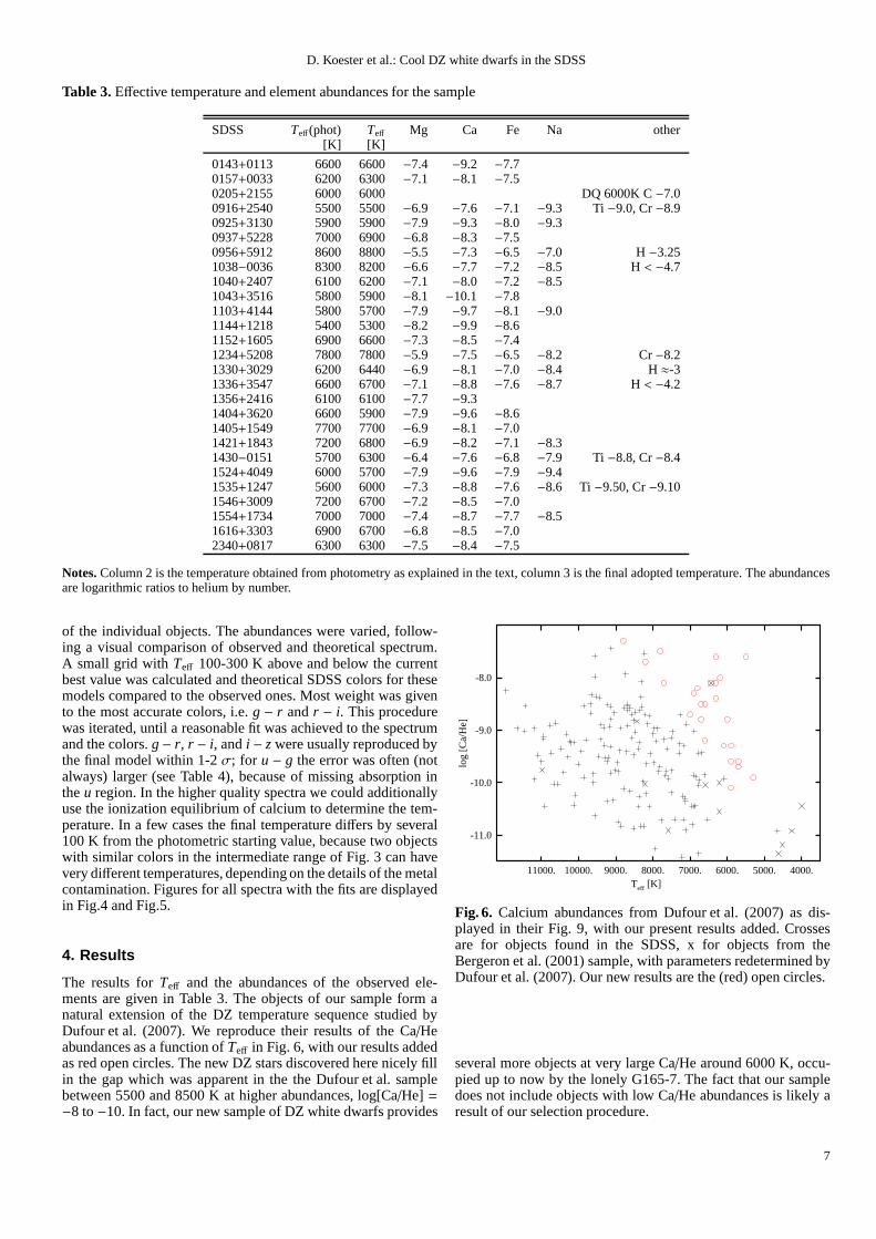
Table 3.Effective temperature and element abundances for the sample
SDSS Teff(phot) Teff Mg Ca Fe Na other[K] [K]
0143+0113 6600 6600 −7.4 −9.2 −7.70157+0033 6200 6300 −7.1 −8.1 −7.50205+2155 6000 6000 DQ 6000K C−7.00916+2540 5500 5500 −6.9 −7.6 −7.1 −9.3 Ti−9.0, Cr−8.90925+3130 5900 5900 −7.9 −9.3 −8.0 −9.30937+5228 7000 6900 −6.8 −8.3 −7.50956+5912 8600 8800 −5.5 −7.3 −6.5 −7.0 H−3.251038−0036 8300 8200 −6.6 −7.7 −7.2 −8.5 H< −4.71040+2407 6100 6200 −7.1 −8.0 −7.2 −8.51043+3516 5800 5900 −8.1 −10.1 −7.81103+4144 5800 5700 −7.9 −9.7 −8.1 −9.01144+1218 5400 5300 −8.2 −9.9 −8.61152+1605 6900 6600 −7.3 −8.5 −7.41234+5208 7800 7800 −5.9 −7.5 −6.5 −8.2 Cr−8.21330+3029 6200 6440 −6.9 −8.1 −7.0 −8.4 H≈-31336+3547 6600 6700 −7.1 −8.8 −7.6 −8.7 H< −4.21356+2416 6100 6100 −7.7 −9.31404+3620 6600 5900 −7.9 −9.6 −8.61405+1549 7700 7700 −6.9 −8.1 −7.01421+1843 7200 6800 −6.9 −8.2 −7.1 −8.31430−0151 5700 6300 −6.4 −7.6 −6.8 −7.9 Ti−8.8, Cr−8.41524+4049 6000 5700 −7.9 −9.6 −7.9 −9.41535+1247 5600 6000 −7.3 −8.8 −7.6 −8.6 Ti−9.50, Cr−9.101546+3009 7200 6700 −7.2 −8.5 −7.01554+1734 7000 7000 −7.4 −8.7 −7.7 −8.51616+3303 6900 6700 −6.8 −8.5 −7.02340+0817 6300 6300 −7.5 −8.4 −7.5
Notes.Column 2 is the temperature obtained from photometry as explained in the text, column 3 is the final adopted temperature. The abundancesare logarithmic ratios to helium by number.
of the individual objects. The abundances were varied, follow-ing a visual comparison of observed and theoretical spectrum.A small grid with Teff 100-300 K above and below the currentbest value was calculated and theoretical SDSS colors for thesemodels compared to the observed ones. Most weight was givento the most accurate colors, i.e.g − r andr − i. This procedurewas iterated, until a reasonable fit was achieved to the spectrumand the colors.g− r, r − i, andi − zwere usually reproduced bythe final model within 1-2σ; for u − g the error was often (notalways) larger (see Table 4), because of missing absorptionintheu region. In the higher quality spectra we could additionallyuse the ionization equilibrium of calcium to determine the tem-perature. In a few cases the final temperature differs by several100 K from the photometric starting value, because two objectswith similar colors in the intermediate range of Fig. 3 can havevery different temperatures, depending on the details of the metalcontamination. Figures for all spectra with the fits are displayedin Fig.4 and Fig.5.
4. Results
The results forTeff and the abundances of the observed ele-ments are given in Table 3. The objects of our sample form anatural extension of the DZ temperature sequence studied byDufour et al. (2007). We reproduce their results of the Ca/Heabundances as a function ofTeff in Fig. 6, with our results addedas red open circles. The new DZ stars discovered here nicely fillin the gap which was apparent in the the Dufour et al. samplebetween 5500 and 8500 K at higher abundances, log[Ca/He] =−8 to−10. In fact, our new sample of DZ white dwarfs provides
4000.5000.6000.7000.8000.9000.10000.11000.
-11.0
-10.0
-9.0
-8.0
Teff [K]
log
[Ca/
He]
Fig. 6. Calcium abundances from Dufour et al. (2007) as dis-played in their Fig. 9, with our present results added. Crossesare for objects found in the SDSS, x for objects from theBergeron et al. (2001) sample, with parameters redetermined byDufour et al. (2007). Our new results are the (red) open circles.
several more objects at very large Ca/He around 6000 K, occu-pied up to now by the lonely G165-7. The fact that our sampledoes not include objects with low Ca/He abundances is likely aresult of our selection procedure.
7
D. Koester et al.: Cool DZ white dwarfs in the SDSS
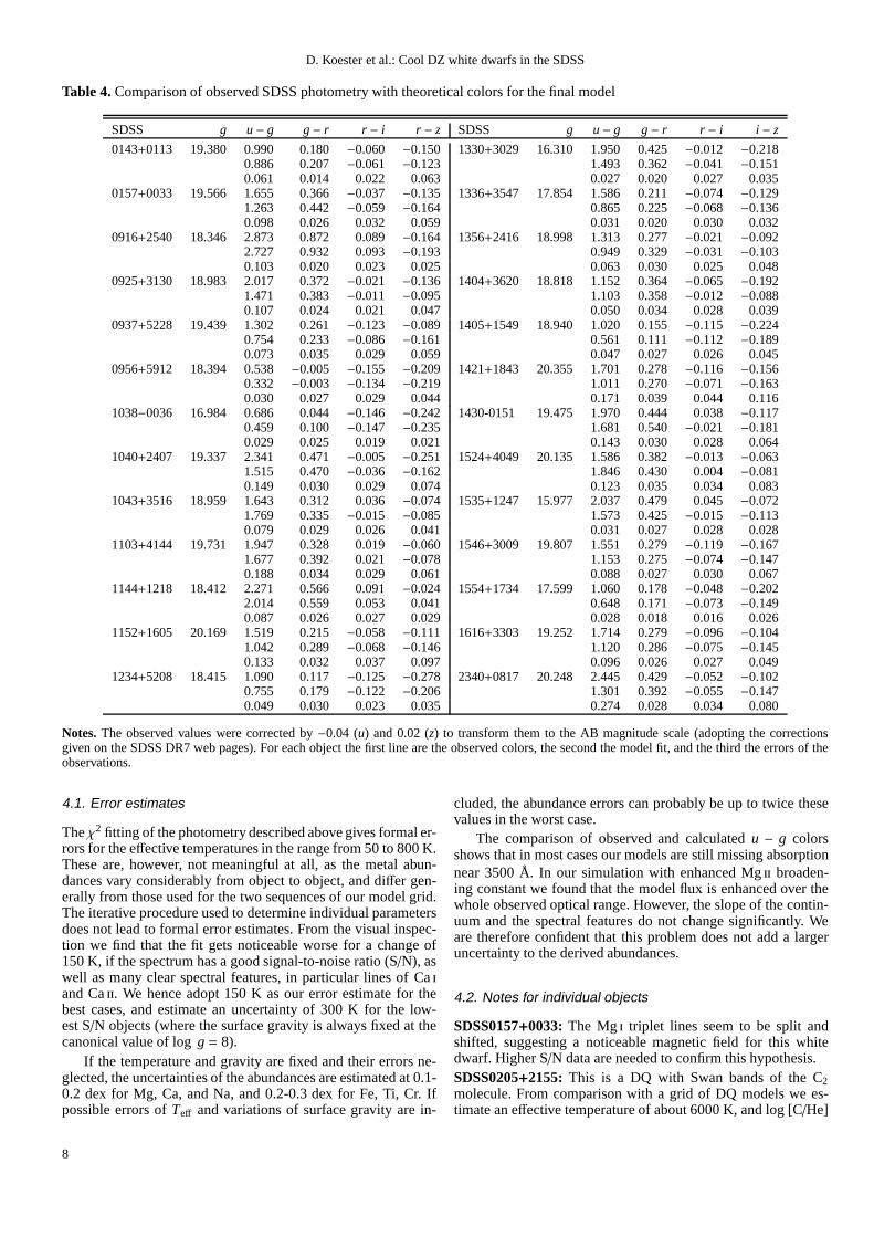
Table 4.Comparison of observed SDSS photometry with theoretical colors for the final model
SDSS g u− g g− r r − i r − z SDSS g u− g g− r r − i i − z
0143+0113 19.380 0.990 0.180 −0.060 −0.150 1330+3029 16.310 1.950 0.425 −0.012 −0.2180.886 0.207 −0.061 −0.123 1.493 0.362 −0.041 −0.1510.061 0.014 0.022 0.063 0.027 0.020 0.027 0.035
0157+0033 19.566 1.655 0.366 −0.037 −0.135 1336+3547 17.854 1.586 0.211 −0.074 −0.1291.263 0.442 −0.059 −0.164 0.865 0.225 −0.068 −0.1360.098 0.026 0.032 0.059 0.031 0.020 0.030 0.032
0916+2540 18.346 2.873 0.872 0.089−0.164 1356+2416 18.998 1.313 0.277 −0.021 −0.0922.727 0.932 0.093 −0.193 0.949 0.329 −0.031 −0.1030.103 0.020 0.023 0.025 0.063 0.030 0.025 0.048
0925+3130 18.983 2.017 0.372 −0.021 −0.136 1404+3620 18.818 1.152 0.364 −0.065 −0.1921.471 0.383 −0.011 −0.095 1.103 0.358 −0.012 −0.0880.107 0.024 0.021 0.047 0.050 0.034 0.028 0.039
0937+5228 19.439 1.302 0.261 −0.123 −0.089 1405+1549 18.940 1.020 0.155 −0.115 −0.2240.754 0.233 −0.086 −0.161 0.561 0.111 −0.112 −0.1890.073 0.035 0.029 0.059 0.047 0.027 0.026 0.045
0956+5912 18.394 0.538 −0.005 −0.155 −0.209 1421+1843 20.355 1.701 0.278 −0.116 −0.1560.332 −0.003 −0.134 −0.219 1.011 0.270 −0.071 −0.1630.030 0.027 0.029 0.044 0.171 0.039 0.044 0.116
1038−0036 16.984 0.686 0.044 −0.146 −0.242 1430-0151 19.475 1.970 0.444 0.038−0.1170.459 0.100 −0.147 −0.235 1.681 0.540 −0.021 −0.1810.029 0.025 0.019 0.021 0.143 0.030 0.028 0.064
1040+2407 19.337 2.341 0.471 −0.005 −0.251 1524+4049 20.135 1.586 0.382 −0.013 −0.0631.515 0.470 −0.036 −0.162 1.846 0.430 0.004 −0.0810.149 0.030 0.029 0.074 0.123 0.035 0.034 0.083
1043+3516 18.959 1.643 0.312 0.036−0.074 1535+1247 15.977 2.037 0.479 0.045−0.0721.769 0.335 −0.015 −0.085 1.573 0.425 −0.015 −0.1130.079 0.029 0.026 0.041 0.031 0.027 0.028 0.028
1103+4144 19.731 1.947 0.328 0.019−0.060 1546+3009 19.807 1.551 0.279 −0.119 −0.1671.677 0.392 0.021 −0.078 1.153 0.275 −0.074 −0.1470.188 0.034 0.029 0.061 0.088 0.027 0.030 0.067
1144+1218 18.412 2.271 0.566 0.091−0.024 1554+1734 17.599 1.060 0.178 −0.048 −0.2022.014 0.559 0.053 0.041 0.648 0.171 −0.073 −0.1490.087 0.026 0.027 0.029 0.028 0.018 0.016 0.026
1152+1605 20.169 1.519 0.215 −0.058 −0.111 1616+3303 19.252 1.714 0.279 −0.096 −0.1041.042 0.289 −0.068 −0.146 1.120 0.286 −0.075 −0.1450.133 0.032 0.037 0.097 0.096 0.026 0.027 0.049
1234+5208 18.415 1.090 0.117 −0.125 −0.278 2340+0817 20.248 2.445 0.429 −0.052 −0.1020.755 0.179 −0.122 −0.206 1.301 0.392 −0.055 −0.1470.049 0.030 0.023 0.035 0.274 0.028 0.034 0.080
Notes.The observed values were corrected by−0.04 (u) and 0.02 (z) to transform them to the AB magnitude scale (adopting the correctionsgiven on the SDSS DR7 web pages). For each object the first lineare the observed colors, the second the model fit, and the third the errors of theobservations.
4.1. Error estimates
Theχ2 fitting of the photometry described above gives formal er-rors for the effective temperatures in the range from 50 to 800 K.These are, however, not meaningful at all, as the metal abun-dances vary considerably from object to object, and differ gen-erally from those used for the two sequences of our model grid.The iterative procedure used to determine individual parametersdoes not lead to formal error estimates. From the visual inspec-tion we find that the fit gets noticeable worse for a change of150 K, if the spectrum has a good signal-to-noise ratio (S/N), aswell as many clear spectral features, in particular lines ofCaiand Caii. We hence adopt 150 K as our error estimate for thebest cases, and estimate an uncertainty of 300 K for the low-est S/N objects (where the surface gravity is always fixed at thecanonical value of logg= 8).
If the temperature and gravity are fixed and their errors ne-glected, the uncertainties of the abundances are estimatedat 0.1-0.2 dex for Mg, Ca, and Na, and 0.2-0.3 dex for Fe, Ti, Cr. Ifpossible errors ofTeff and variations of surface gravity are in-
cluded, the abundance errors can probably be up to twice thesevalues in the worst case.
The comparison of observed and calculatedu − g colorsshows that in most cases our models are still missing absorptionnear 3500 Å. In our simulation with enhanced Mgii broaden-ing constant we found that the model flux is enhanced over thewhole observed optical range. However, the slope of the contin-uum and the spectral features do not change significantly. Weare therefore confident that this problem does not add a largeruncertainty to the derived abundances.
4.2. Notes for individual objects
SDSS0157+0033: The Mgi triplet lines seem to be split andshifted, suggesting a noticeable magnetic field for this whitedwarf. Higher S/N data are needed to confirm this hypothesis.SDSS0205+2155: This is a DQ with Swan bands of the C2molecule. From comparison with a grid of DQ models we es-timate an effective temperature of about 6000 K, and log [C/He]
8

D. Koester et al.: Cool DZ white dwarfs in the SDSS
Table 5.Depth of the convection zone and diffusion time scales
SDSS q Teff Na Mg Ca Ti Cr Fe[K]
0143+0113 −5.3184 6600 5.908 5.916 5.840 5.802 5.824 5.8050157+0033 −5.4374 6300 5.820 5.833 5.736 5.713 5.718 5.6980916+2540 −5.6914 5500 5.633 5.654 5.530 5.517 5.496 5.4720925+3130 −5.4124 5900 5.879 5.896 5.799 5.790 5.789 5.7690937+5228 −5.3260 6900 5.903 5.906 5.828 5.781 5.798 5.7830956+5912 −5.2882 8800 5.972 5.957 5.872 5.808 5.802 5.8101038−0036 −5.1065 8200 6.069 6.080 6.014 5.957 5.938 5.9521040+2407 −5.4839 6200 5.774 5.788 5.684 5.668 5.667 5.6461043+3516 −5.4041 5900 5.885 5.902 5.806 5.797 5.797 5.7771103+4144 −5.4381 5700 5.870 5.890 5.789 5.788 5.779 5.7571144+1218 −5.4411 5300 5.918 5.943 5.841 5.852 5.835 5.8101152+1605 −5.3484 6600 5.894 5.902 5.820 5.782 5.803 5.7821234+5208 −5.2821 7800 5.961 5.946 5.867 5.808 5.811 5.8121330+3029 −5.4610 6440 5.799 5.810 5.706 5.679 5.683 5.6621336+3547 −5.3139 6700 5.924 5.930 5.853 5.811 5.831 5.8131356+2416 −5.3667 6100 5.903 5.918 5.830 5.811 5.819 5.8001404+3620 −5.3800 5900 5.907 5.923 5.832 5.822 5.825 5.8051405+1549 −5.1901 7700 6.026 6.016 5.950 5.893 5.888 5.8901421+1843 −5.3542 6800 5.879 5.885 5.802 5.760 5.779 5.7601430−0151 −5.5399 6300 5.734 5.748 5.634 5.616 5.611 5.5891524+4049 −5.4519 5700 5.859 5.878 5.776 5.774 5.764 5.7421535+1247 −5.4688 6000 5.803 5.819 5.717 5.707 5.703 5.6821546+3009 −5.3588 6700 5.876 5.884 5.801 5.761 5.781 5.7611554+1734 −5.2442 7000 5.978 5.973 5.908 5.856 5.870 5.8641616+3303 −5.3819 6700 5.862 5.870 5.782 5.743 5.762 5.7402340+0817 −5.4007 6300 5.858 5.870 5.779 5.754 5.762 5.742
Notes.q is the fractional depth of the convection zone,q = log Mcvz/M. Columns 4 to 9 give the logarithm of the diffusion time scaleτ for theelements Na to Fe in years.
= −7.0. The decrease of the flux at the blue end may be dueto calcium and possibly iron, which is an interesting possibil-ity, since the current explanation for the DQ stars is dredge-upof carbon from deeper layers (Koester et al. 1982; Pelletieret al.1986). We estimate that the Ca abundance would need to bearound log[Ca/He] = −10.0 to −10.5, but this is pure specula-tion at the moment.SDSS0937+5228: This is a previously known white dwarf(WD0933+526), first identified as a DZ by Harris et al. (2003).SDSS0956+5912: Dufour et al. (2007) findTeff = 8230 K forthis star, whereas we find a somewhat higher temperature fromthe SDSS photometry, continuum slope as well as blue flux. OurCa abundance is also higher by about a factor two.SDSS1038−0036:Our temperature is significantly higher thanthe 6770 K found by Dufour et al. (2007). As can be seen intheir Fig. 7, the Caii lines near 8600 Å are much too weak inthe model. It seems that a higher temperature is a better fit. Thespectrum from DR7 shows unexplained features near 4720 and4865 Å; we have used the reduction of DR4 for the same spec-trum, where the features are absent.SDSS1144+1218:The model fits the photometry very well, butthe slope and absolute scale of the observed spectrum disagree.We consider this to be a calibration problem of the spectrum andthe model in Fig 5 is adjusted with a linear correction.SDSS1152+1605:Although the spectrum is very noisy there aresome indications of possible Zeeman splitting in the strongerlines.SDSS1330+3029:This star is also known as WD 1328+307 andG 165-7. It was analyzed by Dufour et al. (2006) who found it tobe a weakly magnetic (≈ 650kG) DZ white dwarf with Zeemansplitting in lines of Ca, Na, and Fe. We used their parametersTeff
and log g, as well as their abundances and calculated a modelwithout considering a magnetic field. As expected, the lines areslightly weaker and narrower in our model, due to the absenceofthe splitting, but otherwise it agrees very well with their results.SDSS1404+3620: The photometric temperature is very likelytoo high. The continuum slope and Cai/Caii ionization demanda much lowerTeff, which we have adopted here. The theoreticalcolors from the final model agree with the observations.SDSS1535+1247:This is a known white dwarf (WD 1532+129,G137-24), which was classified as DZ by Kawka et al. (2004).Because the spectrum is similar to that of G165-7, they adoptedthe model of Wehrse & Liebert (1980) for that star withTeff =
7500 K and found metal abundances of≈ 1/100 solar. Theynote, however, that a fit to theVJH photometry results inTeff= 6000±400 K. The u − g and g − r colors are similar toSDSS1330+3029, yet the slope of the spectra is quite different.Also, adding thei andz magnitude for the photospheric fit re-sults in significantly lower temperature. The best compromiseusing the resonance and excited lines from the two ionizationstages isTeff = 6000 K, in agreement with the photometric resultof Kawka et al. (2004). The theoreticalgriz photometry for thefinal model agrees well with the observations (Table 4).SDSS1546+3009: This object may be weakly magnetic, withsplittings and shifts apparent in many metal lines. A higherS/Nspectrum is needed for confirmation.
5. Element abundances, diffusion, and accretion
Heavy elements in a helium-dominated atmosphere will sink outof the outer, homogeneously mixed convection zone into deeperlayers. The abundance observed depends on the interplay of ac-
9

D. Koester et al.: Cool DZ white dwarfs in the SDSS
cretion from the outside and diffusion at the bottom of the con-vection zone. These diffusion time scales can be calculated forall objects using the methods and input physics as describedinKoester & Wilken (2006) and Koester (2009). The data are col-lected in Table 5.
The size of the convection zone, and the diffusion time scalesdepend on the effective temperature, which determines the stellarstructure. In addition it depends on the metal composition of theatmosphere, because the atmospheric data at Rosseland opticaldepth 50 are used as outer boundary conditions for the envelopecalculations. However, the total range of time scales over all ob-jects and all elements only varies within a factor of≈ 4, from3 105 to 1.2 106 years.
As discussed in Koester (2009), the interpretation of ob-served abundances, and their relation to the abundances in theaccreted material depends on the identification of the currentphase within the accretion/diffusion scenario: initial accretion,steady state, or final decline. Except for the case of hotter DAZ,with diffusion time scales of a few years or less, we generallydo not know in which phase we observe the star. The currentlyfavored source for the accreted matter is a dusty debris disk,formed by the tidal disruption of planetary rocky material.Thelifetime of such a debris disk is highly uncertain; estimates putit around 1.5 105 yrs (Jura 2008; Kilic et al. 2008). If the life-time is really that short, the steady state phase would neverbereached for the cool DZ analyzed here. The observable abun-dances would be close to the accreted abundances during theinitial accretion phase. If the accretion rate declines exponen-tially, this abundance pattern could persist for a longer period.If the accretion is switched off abruptly, the element abundanceswould diverge, according to their diffusion time scales.
The differences between the time scales of the four elementsMg, Na, Ca, Fe, which are observed in most objects, are at mosta factor of 1.4. Given the relatively large differences betweenthe diffusion time scales of Mg and Fe, is possible to attributethe scatter of the Fe/Mg ratio to differences in the time sincethe accretion episode? Let us assume for a moment that all ob-jects have reached similar abundances when the accretion stops.The observed range in Mg abundances of 2.7 dex would, underthis assumption, be due to an exponential decline for a durationof 6.22τ(Mg). During this time the Mg/Fe ratio would changeby a factor of 12 or 1.1 dex, and we would expect a correlationbetween Mg abundance and the Fe/Mg ratio. This model is obvi-ously a strong oversimplification, but at least in a statistical senseit might be true that objects with lower overall metal abundancemight have spent more time since the accretion stopped. Is suchan effect observable?
Fig. 7 shows the comparison for the Na/Mg, Ca/Mg, andFe/Mg ratios. There is no evolution visible in the first two ratios.For Na/Mg this is expected, since the diffusion time scales arevery similar and the ratio should always stay close to the accre-tion ratio. This would imply that the Na/Mg ratio in the accretedmaterial can vary by much more than a factor of ten.
If anything, the Fe/Mg ratio shows an increase, in spite ofthe shorter time scales of iron. This means that the Mg abun-dance cannot be interpreted as an indicator of time since accre-tion; more likely the accretion reaches different values in differ-ent objects. The variation by a factor of ten in the Fe/Mg ratiocould then be explained by subsequent diffusion.
The above considerations are rather speculative and needto be taken with a grain of salt. Abundance errors in individ-ual objects could add up to 0.5 dex, and the theoretical diffu-sion time scales use several approximations (Koester 2009)– wecannot exclude that the uncertainties are as high as a factorof
-8.00-7.50-7.00-6.50-6.00
-2.00
-1.00
0.00
log [Mg/He]
log
[met
al/M
g]
Fig. 7. Ca/Mg (red circles), Fe/Mg (black crosses), and Na/Mg(blue x) as a function of the magnesium abundance.
Table 6. Average logarithmic abundance ratios for Fe/Mg,Ca/Mg, Na/Mg, and Na/Ca
Data [Fe/Mg] [Ca/Mg] [Na/Mg] [Na/Ca]
average −0.35 −1.42 −1.56 −0.19σ(mean) 0.06 0.06 0.09 0.08
σ(distribution) 0.38 0.33 0.37 0.58bulk Earth −0.13 −1.21 −1.77 −0.56
solar −0.10 −1.26 −1.36 −0.10
Notes.σ(mean) is the statistical error of the mean value,σ(distribution)is the width of the distribution.
1.5. Because the time scales for the different elements given inTable 5 are very similar, such small changes could even invertthe trends discussed above.
An alternative interpretation could be to assume that themetal ratios are all still close to the accreted, assumed to be sim-ilar in all objects, and that the observed distribution is causedby uncertainties of the abundances and atmospheric parameters(e.g. log g). Table 6 collects relevant data for mean values anddistributions of the metal-to-Mg abundance ratios. The width ofthe distributions could be completely explained, assumingtypi-cal errors of 0.15 dex for Mg, and 0.25 dex for Fe, Ca, and Na.In view of the error discussion above this is not implausible.
6. Conclusions
We have identified 26 DZ and one DQ stars across and below themain sequence in theu − g vs. g − r SDSS two-color diagram,most of which are new detections. A search routine tailored tothe specific spectral features observed in these DZ was needed toavoid the confusion by the much more numerous main sequencestars and QSOs in this region. From our analysis with theoret-ical model atmospheres, which uses newly developed line pro-files for the strongly broadened Ca and Mg lines, we determinedthe white dwarf temperatures and abundances for the pollutingelements Ca, Mg, Fe, Na, and in a few cases Cr and Ti. Thetemperatures and abundances show that these objects form a se-quence which continues that of the hotter DZs in the sample ofDufour et al. (2007). The new objects fill the deficiency of ob-jects withTeff<∼ 8000 K at high Ca/He abundances, which wasapparent in that work. We do not find new low-abundance DZ,
10

D. Koester et al.: Cool DZ white dwarfs in the SDSS
which is most likely a consequence of the design of our searchalgorithm.
Very little is known for these DZ regarding their currentphase in the accretion/diffusion scenario. However, if the accre-tion is, or was, from a circumstellar dust disk, it is unlikely thata steady state phase occurs, since the diffusion time scales are ofthe same order as the expected lifetime of such a disk. Becausethe diffusion time scales of the observed elements are very simi-lar, we might expect that the metal-to-metal ratios are not too farfrom those in the accreted matter, and we compare the averagevalues of these elements in the bulk Earth (Allegre et al. 1995)and the Sun (Asplund et al. 2009) in Table 6. The average abun-dance ratios found for our DZ sample are similar to those of bothbulk Earth and the Sun, with the Na/Ca ratio slightly favoring thesolar abundance ratio.
An important element for a distinction between differentsources would be carbon, which is not detected in our sample.This element is about a factor of 100 under-abundant in the bulkEarth, compared to the Sun and the interstellar medium. The DQstar SDSS0205+2155 demonstrates that log[C/He] = −7 pro-duces clearly visible Swan bands. However, with the metal pol-lution in the other objects, the pressure and the transparency inthe atmosphere are lower (due to more free electrons), and thetypical upper limits are log [C/He] = −5.5 to −6.0, which istoo high to distinguish between bulk Earth and solar/ISM car-bon abundances.
Another critical element for all possible explanations is hy-drogen. We note that in all objects the abundance of hydrogenrelative to the metals is less than the solar value, even in theone case where it is detected. This is consistent with accre-tion of predominantly volatile-depleted material, since hydro-gen accreted from the interstellar matter or from circumstellarwater/ice would stay in the convection zone and can only accu-mulate with time.
In the case of the DBZ star GD40, Klein et al. (2010) wereable to deduce very detailed conclusions from a comparison ofphotospheric abundances with those of various solar systembod-ies. The abundance ratios we obtain here roughly follow thatofthe bulk Earth. However, the remaining uncertainties of surfacegravity, abundances, and time since the last accretion event donot allow us to draw any further conclusions in the present study.High resolution, high S/N observations and extending the spec-tral coverage at least to 3200 Å, or better to 2700 Å (to coverthe Mgii/Mg i resonance lines) are needed to refine the elementabundances and detect the very crucial element silicon, andifpossible carbon and oxygen.
We can, however, estimate a lower limit for the total ac-creted mass based on the available data for the convection zone.For SDSS0956+5912, which has the highest metal pollution,we find a total mass for theobservedmetals Mg, Ca, Fe, Naof 1.5 1023g. Adding oxygen with the same ratio to Mg as inGD40 (Klein et al. 2010) this number becomes 4.8 1023g, evenmore than in the extremely heavily polluted SDSS0738+1835(Dufour et al. 2010). The total amount of H in the convectionzone is 1.0 1024g. For SDSS1144+1218, which has the lowestabundances, these numbers are 3.2 1020g (observed metals), and7.9 1020g (including oxygen). These masses span the range ofthe most massive asteroids in our own planetary system. Theseare the absolute minimum of the accreted masses – depending onhow long ago the accretion ended, these masses can be at leasttwo orders of magnitude larger, which will require minor plan-ets much larger than known in the Solar system. Another openquestion, recently discussed by Farihi et al. (2011) in the con-text of G77-50, a DAZ of similar low temperature, is how such
a very massive asteroid is suddenly driven into its host starfroman orbit apparently stable over the past 5 Gyrs.
Acknowledgements.This work has made extensive use of VALD, theVienna Atomic Line Database (Piskunov et al. 1995; Ryabchikova et al. 1997;Kupka et al. 1999, 2000)
ReferencesAbazajian, K. N., Adelman-McCarthy, J. K., Agueros, M. A.,et al. 2009, 182,
543Allard, N. & Kielkopf, J. 1982, Reviews of Modern Physics, 54, 1103Allard, N. F., Allard, F., Hauschildt, P. H., Kielkopf, J. F., & Machin, L. 2003,
A&A, 411, L473Allegre, C. J., Poirier, J., Humler, E., & Hofmann, A. W. 1995, Earth and
Planetary Science Letters, 134, 515Asplund, M., Grevesse, N., Sauval, A. J., & Scott, P. 2009, ARA&A, 47, 481Bergeron, P., Leggett, S. K., & Ruiz, M. T. 2001, ApJS, 133, 413Czuchaj, E., Rebentrost, F., Stoll, H., & Preuss, H. 1996, Chemical Physics, 207,
51Debes, J. H. & Sigurdsson, S. 2002, ApJ, 572, 556Dufour, P., Bergeron, P., Liebert, J., et al. 2007, ApJ, 663,1291Dufour, P., Bergeron, P., Schmidt, G. D., et al. 2006, ApJ, 651, 1112Dufour, P., Kilic, M., Fontaine, G., et al. 2010, ApJ, 719, 803Dupuis, J., Fontaine, G., Pelletier, C., & Wesemael, F. 1992, ApJS, 82, 505Dupuis, J., Fontaine, G., Pelletier, C., & Wesemael, F. 1993a, ApJS, 84, 73Dupuis, J., Fontaine, G., & Wesemael, F. 1993b, ApJS, 87, 345Farihi, J., Barstow, M. A., Redfield, S., Dufour, P., & Hambly, N. C. 2010a,
MNRAS, 404, 2123Farihi, J., Dufour, P., Napiwotzki, R., & Koester, D. 2011, MNRAS, 358, ArXiv
e-prints 1101.2203Farihi, J., Jura, M., Lee, J., & Zuckerman, B. 2010b, ApJ, 714, 1386Farihi, J., Jura, M., & Zuckerman, B. 2009, ApJ, 694, 805Gansicke, B. T., Koester, D., Marsh, T. R., Rebassa-Mansergas, A., &
Southworth, J. 2008, MNRAS, 391, L103Gansicke, B. T., Marsh, T. R., & Southworth, J. 2007, MNRAS,380, L35Gansicke, B. T., Marsh, T. R., Southworth, J., & Rebassa-Mansergas, A. 2006,
Science, 314, 1908Gansicke, B. T., Koester, D., Girven, J., Marsh, T. R., & Steeghs, D. 2010,
Science, 327, 188Harris, H. C., Liebert, J., Kleinman, S. J., et al. 2003, AJ, 126, 1023Holberg, J. B., Barstow, M. A., & Green, E. M. 1997, ApJ, 474, L127Jura, M. 2003, ApJ, 584, L91Jura, M. 2006, ApJ, 653, 613Jura, M. 2008, AJ, 135, 1785Kawka, A., Vennes, S., & Thorstensen, J. R. 2004, AJ, 127, 1702Kilic, M., Farihi, J., Nitta, A., & Leggett, S. K. 2008, AJ, 136, 111Klein, B., Jura, M., Koester, D., Zuckerman, B., & Melis, C. 2010, ApJ, 709,
950Koester, D. 2009, A&A, 498, 517Koester, D., Provencal, J., & Shipmann, H. L. 1997, A&A, 320,L57Koester, D., Weidemann, V., & Zeidler-KT, E. M. 1982, A&A, 116, 147Koester, D. & Wilken, D. 2006, A&A, 453, 1051Kuiper, G. P. 1941, PASP, 53, 248Kupka, F., Piskunov, N., Ryabchikova, T. A., Stempels, H. C., & Weiss, W. W.
1999, A&AS, 138, 119Kupka, F. G., Ryabchikova, T. A., Piskunov, N. E., Stempels,H. C., & Weiss,
W. W. 2000, Baltic Astronomy, 9, 590Monteiro, T. S., Cooper, I. L., Dickinson, A. S., & Lewis, E. L. 1986, Journal of
Physics B Atomic Molecular Physics, 19, 4087Pelletier, C., Fontaine, G., Wesemael, F., Michaud, G., & Wegner, G. 1986, ApJ,
307, 242Piskunov, N. E., Kupka, F., Ryabchikova, T. A., Weiss, W. W.,& Jeffery, C. S.
1995, A&AS, 112, 525Richards, G. T., Fan, X., Newberg, H. J., et al. 2002, 123, 2945Ryabchikova, T. A., Piskunov, N. E., Kupka, F., & Weiss, W. W.1997, Baltic
Astronomy, 6, 244Sion, E. M., Holberg, J. B., Oswalt, T. D., McCook, G. P., & Wasatonic, R. 2009,
138, 1681Unsold, A. 1968, Physik der Sternatmospharen (Berlin: Springer-Verlag)von Hippel, T., Kuchner, M. J., Kilic, M., Mullally, F., & Reach, W. T. 2007,
ApJ, 662, 544Walkup, R., Stewart, B., & Pritchard, D. E. 1984, Phys. Rev. A, 29, 169Wehrse, R. & Liebert, J. 1980, A&A, 86, 139Zeidler-KT, E. M., Weidemann, V., & Koester, D. 1986, A&A, 155, 356
11