Convolutional Neural Networks for CroatianTraffic Signs Recognition

Vedran Vukotic, Josip Krapac and Siniša ŠegvicUniversity of Zagreb - Faculty of Electrical Engineering and Computing

Zagreb, HR-10000, CroatiaEmail: vevukotic@gmail.com

Abstract—We present an approach to recognition of Croatiantraffic signs based on convolutional neural networks (CNNs). Alibrary for quick prototyping of CNNs, with an educational scope,is first developed1. An architecture similar to LeNet-5 is thencreated and tested on the MNIST dataset of handwritten digitswhere comparable results were obtained. We analyze the FER-MASTIF TS2010 dataset and propose a CNN architecture fortraffic sign recognition. The presented experiments confirm thefeasibility of CNNs for the defined task and suggest improvementsto be made in order to improve recognition of Croatian trafficsigns.

I. INTRODUCTION

Traffic sign recognition is an example of the multipleclasses recognition problem. Classical approaches to this prob-lem in computer vision typically use the following well-known pipeline: (1) local feature extraction (e.g. SIFT), (2)feature coding and aggregation (e.g. BOW) and (3) learning aclassifier to recognize the visual categories using the chosenrepresentation (e.g. SVM). The downsides of these approachesinclude the suboptimality of the chosen features and the needfor hand-designing them.

CNNs approach this problem by learning meaningful repre-sentations directly from the data, so the learned representationsare optimal for the specific classification problem, thus elim-inating the need for hand-designed image features. A CNNarchitecture called LeNet-5 [1] was successfully trained forhandwritten digits recognition and tested on the MNIST dataset[2] yielding state-of-art results at the time. An improved andlarger CNN was later developed [3] and current state-of-the-artresults on the GTSRB dataset [4] were obtained.

Following the results by [3], we were motivated to evaluatea similar architecture on the Croatian traffic signs dataset FER-MASTIF TS2010 [5]. To do so, we first developed a librarythat would allow us to test different architectures easily. Afterdifferent subsets were tested for successful convergence, anarchitecture similar to LeNet-5 was built and tested on theMNIST dataset, yielding satisfactory results. Following thesuccessful reproduction of a handwritten digit classifier (anerror rate between 1.7% and 0.8%, where LeNet-X architec-tures yield their results), we started testing architectures for asubset of classes of the FER-MASTIF TS2010 dataset.

In the first part of this article, CNNs are introduced andtheir specifics, compared to classical neural networks, are pre-sented. Ways and tricks for training them are briefly explained.

1Available at https://github.com/v-v/CNN/

In the second part the datasets are described and the choiceof a subset of classes for the FER-MASTIF TS2010 dataset iselaborated. In the last part of the paper, the experimental setupis explained and the results are discussed. Finally, commonproblems are shown and suggestions for future improvementsare given.

II. ARCHITECTURAL SPECIFICS OF CNNS

Convolutional neural networks represent a specialization ofgeneric neural networks, where the individual neurons form amathematical approximation of the biological visual receptivefield [6]. Visual receptive fields correspond to small regions ofthe input that are processed by the same unit. The receptivefields of the neighboring neurons overlap, allowing thus robust-ness of the learned representation to small translations of theinput. Each receptive field learns to react to a specific feature(automatically learned as a kernel). By combining many layers,the network forms a classifier that is able to automatically learnrelevant features and is less prone to translational variancein data. In this section, the specific layers (convolutional andpooling layers) of CNNs will be explained. A CNN is finallybuilt by combining many convolutional and pooling layers,so the number of output in each successive layer grows,while size of images on the output is reducing. The outputof the last CNN layer is a vector image representation. Thisimage representation is then classified using a classical fully-connected MLP [3], or another classifier, e.g. an RBF network[1]).

INPUT IMAGE FEATURE MAPS FEATURE MAPS

FEATU

RE M

APS

HID

DEN

LAYER

OU

TPU

T LA

YER

KER

NELS

{ { {CONVOLUTION POOLING FULLY CONNECTED LAYERS

Fig. 1: Illustration of the typical architecture and the differentlayers used in CNNs. Many convolutional and pooling layersare stacked. The final layers consist of a fully connectednetwork.

A. Feature maps

Fig. 2 shows a typical neuron (a) and a feature map (b).Neurons typically output a scalar, while feature maps represent

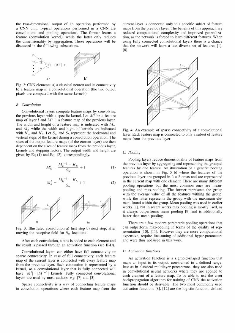
the two-dimensional output of an operation performed bya CNN unit. Typical operations performed in a CNN areconvolutions and pooling operations. The former learns afeature (convolution kernel), while the latter only reducesthe dimensionality by aggregation. These operations will bediscussed in the following subsections.

b

a) b)

Σ

x1

x2

...xn

σ(∙) y

w1

w2

wn

.

Fig. 2: CNN elements: a) a classical neuron and its connectivityb) a feature map in a convolutional operation (the two outputpixels are computed with the same kernels)

B. Convolution

Convolutional layers compute feature maps by convolvingthe previous layer with a specific kernel. Let M l be a featuremap of layer l and M l−1 a feature map of the previous layer.The width and height of a feature map is indicated with Mw

and Mh while the width and hight of kernels are indicatedwith Kw and Kh. Let Sw and Sh represent the horizontal andvertical steps of the kernel during a convolution operation. Thesizes of the output feature maps (of the current layer) are thendependent on the sizes of feature maps from the previous layer,kernels and stepping factors. The output width and height aregiven by Eq (1) and Eq. (2), correspondingly.

M lw =

M l−1w −Kw

Sw+ 1 (1)

M lh =

M l−1h −Kh

Sh+ 1 (2)

FEATURE M

AP Ml-1

KERNEL

FEATURE M

AP M

l

FEATURE M

AP Ml-1

KERNEL

FEATURE M

AP M

l

a) b)

b

b

Fig. 3: Illustrated convolution a) first step b) next step, aftermoving the receptive field for Sw locations

After each convolution, a bias is added to each element andthe result is passed through an activation function (see II-D).

Convolutional layers can either have full connectivity orsparse connectivity. In case of full connectivity, each featuremap of the current layer is connected with every feature mapfrom the previous layer. Each connection is represented by akernel, so a convolutional layer that is fully connected willhave |M l| · |M l−1| kernels. Fully connected convolutionallayers are used by most authors, e.g. [7] and [3].

Sparse connectivity is a way of connecting feature mapsin convolution operations where each feature map from the

current layer is connected only to a specific subset of featuremaps from the previous layer. The benefits of this approach arereduced computational complexity and improved generaliza-tion, as the network is forced to learn different features. Whenusing fully connected convolutional layers there is a chancethat the network will learn a less diverse set of features [1],[8].

b

b

b

Fig. 4: An example of sparse connectivity of a convolutionallayer. Each feature map is connected to only a subset of featuremaps from the previous layer

C. Pooling

Pooling layers reduce dimensionality of feature maps fromthe previous layer by aggregating and representing the groupedfeatures by one feature. An illustration of a generic poolingoperation is shown in Fig. 5 b) where the features of theprevious layer are grouped in 2× 2 areas and are representedin the current map with one element. There are many differentpooling operations but the most common ones are mean-pooling and max-pooling. The former represents the groupwith the average value of all the features withing the group,while the latter represents the group with the maximum ele-ment found within the group. Mean pooling was used in earlierworks [1], but in recent works max pooling is mostly used, asit always outperforms mean pooling [9] and is additionallyfaster than mean pooling.

There are a few modern parametric pooling operations thatcan outperform max-pooling in terms of the quality of rep-resentation [10], [11]. However they are more computationalexpensive, require fine-tuning of additional hyper-parametersand were thus not used in this work.

D. Activation functions

An activation function is a sigmoid-shaped function thatmaps an input to its output, constrained to a defined range.Just as in classical multilayer perceptrons, they are also usedin convolutional neural networks where they are applied toeach element of a feature map. To be able to use the errorbackpropagation algorithm for training of CNN the activationfunction should be derivable. The two most commonly usedactivation functions [8], [12] are the logistic function, defined

SAME KERNEL

a) b)

Fig. 5: a) Weight sharing in convolutional layers, the samekernel is used for all the elements within a feature map b) ageneric pooling operation

in Eq. (3) and a scaled tanh sigmoidal function, defined in Eq.(4)

f(x) =2

1 + e−βx− 1 (3)

f(x) = 1.7159 tanh

(2

3x

)(4)

Weights and kernel elements are randomly initialized byusing a uniform distribution [13]. However, the samplinginterval depends on the choice of the activation function. Forthe logistic function, the interval is given in (5), while for thescaled tanh sigmoidal function the interval is given in (6). Inthose equations nin indicates the number of neurons (or featuremap elements) in the previous layer, while nout indicates thenumber of neurons (or feature map elements) in the currentlayer. Improper initialization may lead to poor convergence ofthe network.

[√6

nin + nout,

√6

nin + nout

](5)

[−4

√6

nin + nout, 4

√6

nin + nout

](6)

III. TRAINING CNNS

In supervised training, convolutional neural networks aretypically trained by the Backpropagation algorithm. The algo-rithm is the same as for multilayer perceptrons but is extendedfor convolutional and pooling operations.

A. Backpropagation for convolutional layers

For convolutional layers, the backpropagation algorithm isthe same as for multilayer perceptrons (if every element ofa feature map is treated as a neuron and every element ofa kernel is treated as a weight) with the only exception thatweights are shared inside a feature map. Fig. 5 a) illustratesweight sharing in a convolution between two feature maps.The weight sharing easily fits into backpropagation algorithm:because multiple elements of the feature map contribute to theerror, the gradients from all these elements contribute to thesame set of weights.

B. Backpropagation for pooling layers

Pooling layers require a way to reverse the pooling oper-ation and backpropagate the errors from the current featuremap to the previous one. For the case of max-pooling, theerror propagates to the location where the maximal featureis located while the other locations receives an error of zero.For mean-pooling, the error is equally distributed within thelocations that were grouped together in the forward pass andcan be expressed as E′ = E⊗ 1, where E′ is the error of theprevious layer, E the error of the current layer and ⊗ representsthe Kronecker product.

IV. IMPROVING LEARNING

A. Backpropagation with momentum

The classical Backpropagation algorithm uses a globallearning rate η to scale the weight updates. This modifiedversion scales the learning rate dynamically depending on thepartial derivative in the previous update. The method is definedin the Eq. (7), where α represents the amortization factor(typical values between 0.9 and 0.99).

∆w(t) = α∆w(t− 1)− η ∂E∂w

(t) (7)

B. Adding random transformations

Generalization can be improved by increasing the numberof training samples. However that usually requires additionalhuman effort for collection and labelling. Adding randomtransformations can increase the generalization capability ofa classifier without additional effort. There are two main waysfor deploying random transformations into a system: (1) byintegrating them into the network, after the input layers [3]or (2) by generating additional samples and adding them tothe training set [14]. In this work we opted for generatingadditional samples since the code is currently not optimizedfor speed, and adding an additional task to be performed foreach iteration would further slow the learning process.

C. Dropout

A typical approach in machine learning when improvinggeneralization consists of combining different architectures.However, that can be computationally quite expensive. Thedropout method suggests randomly disabling some hiddenunits during training, thus generating a large set of combinedvirtual classifiers without the computational overhead [15].For a simple multilayer perceptron with N neurons in onehidden layer, 2N virtual architectures would be generated whenapplying dropout. Usually, half the units are disabled in eachlearning iteration and that is exactly what we used in this work.

V. DATASETS

Two datasets were used in this work. The MNIST dataset ofhandwritten digits [2] and the FER-MASTIF TS2010 datasetof Croatian traffic signs [5] [16].

A. MNIST

The MNIST dataset consists of 10 classes (digits from 0to 9) of 28× 28 grayscale images. It is divided into a trainingset of 60000 samples and a testing set of 10000 samples. Thedataset was unaltered except for preprocessing it to a mean ofzero and unit variance.

Fig. 6: Samples from the MNIST dataset

B. FER-MASTIF TS2010

This dataset consists of 3889 images of 87 different trafficsigns and was collected with a vehicle mounted video cameraas a part of the MASTIF (Mapping and Assessing the State ofTraffic InFrastructure) project. In [17], images were selectedby the frame number and split in two different sets, a trainingset and a test set. This method ensured that images of the sametraffic sign do not occur in both sets. The sizes varies from 15pixels to 124 pixels. We opted for classes containing at least20 samples of sizes greater or equal to 44× 44. Fig. 8 showsthe nine classes that met that criteria.

Fig. 7: Part of the histogram showing the number of samplesbigger or equal to 44×44 for two sets. The black line separatesthe classes that we chose (more than 20 samples) for ourexperiments.

Each sample was first padded with 2 pixels on each side(thus expanding their size to 48×48) to allow the convolutionallayers to relevant features close to the border. The selectedsubset of samples was then expanded by applying randomtransformations until 500 samples per class were obtained.

The random transformations applied are: (1) rotation sampledfrom N (0, 5◦) and (2) translation of each border (that servesthe purpose of both scaling and translation), sampled fromN (0, 1px). In the end, every sample was preprocessed so thatit has a mean of zero and unit variance.

Fig. 8: The selected 9 classes of traffic signs.

VI. EXPERIMENTS AND RESULTS

Different architectures were built and evaluated for eachdataset. In the following section the architectural specifics ofconvolutional neural networks for each experiment are defined,their performance is illustrated and results are discussed.

A. MNIST

The following architecture was built:

• input layer - 1 feature map 32× 32• first convolutional layer - 6 feature maps 28× 28• first pooling layer - 6 feature maps 14× 14• second convolutional layer - 16 feature maps 10×10• second pooling layer - 16 feature maps 5× 5• third convolutional layer - 100 feature maps 1× 1• hidden layer - 80 neurons• output layer - 10 neurons

The network was trained by stochastic gradient descentwith 10 epochs of 60000 iterations each. No dropout and norandom transformations were used. Such network yielded aresult of 98.67% precision on the MNIST test set. Table Ishows the obtained confusion matrix. The three most commonmistakes are as shown in Fig. 9. It can be noticed that samplesthat were mistaken share a certain similarity with the wronglypredicted class.

Predicted class0 1 2 3 4 5 6 7 8 9

Act

ual

clas

s

0 973 0 1 0 0 0 3 1 2 01 0 1127 4 1 0 0 1 0 2 02 3 0 1020 0 0 0 0 4 5 03 0 0 2 992 0 6 0 3 5 24 1 0 1 0 963 0 4 0 2 115 1 0 0 3 0 884 1 1 0 26 10 2 0 0 1 2 943 0 0 07 0 1 7 2 0 0 0 1014 1 38 2 0 1 0 1 1 1 3 962 39 3 2 0 3 1 3 1 4 3 989

TABLE I: Confusion matrix for the MNIST dataset

a) 9

b) 0

c) 2

PREDICTED CLASS SAMPLES

Fig. 9: The three most common errors on the MNIST dataset:a) number 4 classified as 9, b) number 6 classified as 0, c)number 7 classified as 2

B. FER-MASTIF TS2010

The following architecture was built:

• input layer - 3 feature maps 48× 48• first convolutional layer - 10 feature maps 42× 42• first pooling layer - 10 feature maps 21× 21• second convolutional layer - 15 feature maps 18×18• second pooling layer - 15 feature maps 9× 9• third convolutional layer - 20 feature maps 6× 6• third pooling layer - 10 feature maps 3× 3• fourth convolutional layer - 40 feature maps 1× 1• hidden layer - 80 neurons• output layer - 9 neurons

The network was trained with 20 epochs of 54000 iterationseach by stochastic gradient descent. Random transformationswere used (as defined in Section V) while dropout was notused. The trained network yielded a result of 98.22% on thetest set. Table II shows the full confusion matrix on the testset and Fig. 10 shows the three most common errors made bythe network.

Predicted classC02 A04 B32 A33 C11 B32 A05 B46 A03

Act

ual

clas

s

C02 100 0 0 0 0 0 0 0 0A04 0 99 0 0 0 0 1 0 0B32 0 0 97 3 0 0 0 0 0A33 0 0 0 100 0 0 0 0 0C11 0 0 0 0 100 0 0 0 0B31 0 0 0 0 0 100 0 0 0A05 0 0 0 0 0 0 98 0 2B46 0 0 0 0 0 0 0 100 0A03 0 3 0 0 0 0 7 0 90

TABLE II: Confusion matrix obtained on the FER-MASTIFTS2010 dataset

a)

b)

c)

A05

A04

A33

PREDICTEDCLASS

SAMPLES

Fig. 10: The three most common errors on the FER-MASTIFTS2010 dataset a) A03 predicted as A05, b) A03 predicted asA04, c) B32 predicted as A33

C. FER-MASTIF TS2010 with smaller samples included

Fig. 11 shows the distribution of sample sizes (of the cho-sen 9 classes) in the FER-MASTIF TS2010 set. To determinethe influence of sample size to the classification error, wescaled all samples to the same size (44 × 44 with paddingleading to an input image of 48 × 48), matching the inputof the network. In the previous experiment, samples smallerthan 44 × 44 that were not used. However, in the followingexperiment they were included in the test set by upscaling tothe required size.

Fig. 11: Number of samples of different sizes (within the 9chosen classes)

Fig. 12 shows the percentage of misclassified samples fordifferent sizes. It can be seen that samples bigger than 45×45produce significantly lower error rates than smaller samples,thus confirming our choice of the input dimensionality to theCNN.

Fig. 12: Dependency of the error rate on the sample size. (Thevertical line denotes the limit of 44px from where samples forthe experiments in subsections A and B were taken.)

D. FER-MASTIF TS2010 with dropout

The same architecture was trained again with dropout inthe final layers. We used the previously defined 9 classesand, again, only samples larger than 44 × 44. Using dropoutimproved the network generalization capability that yielded aresult of 99.33% precision.

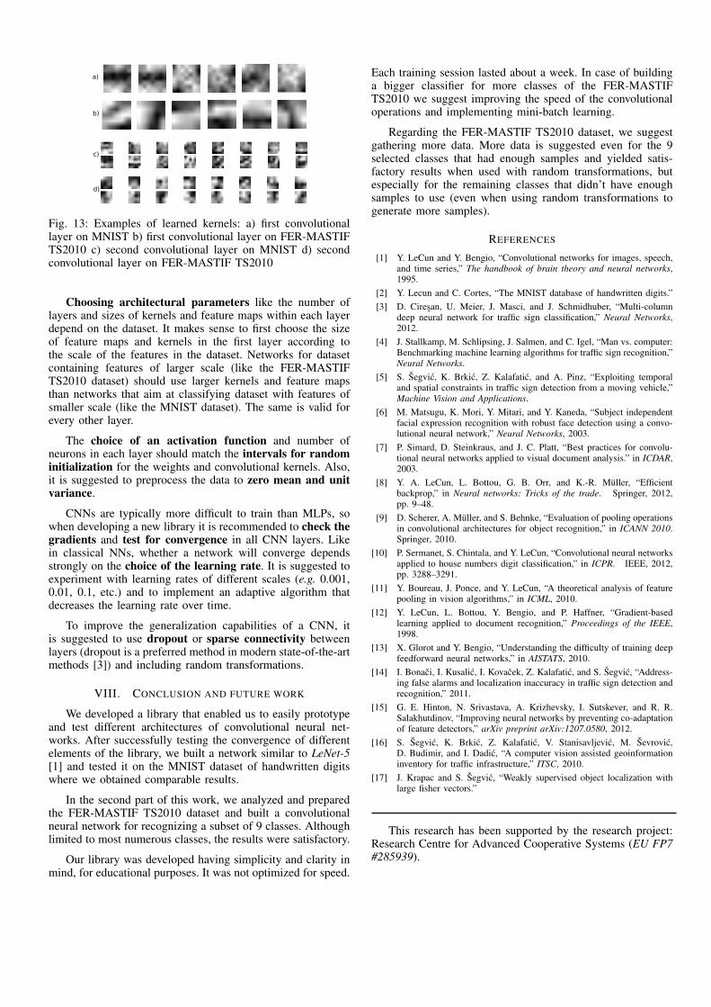
E. Comparison of learned kernels

Fig. 13 shows a few learned convolutional kernels fromthe first and second convolutional layers on the two differentdatasets. It is clearly visible that the network adapted to thedataset and learned different distinct features for each dataset.

VII. COMMON PROBLEMS IN TRAINING CNNS

CNNs are difficult to train because they have many hyper-parameters and learning procedure parameters, which needto be set correctly in order for learning to converge. In thissection, we discuss a few issues that we had during thedevelopment of our library and the two networks.

a)

b)

c)

d)

Fig. 13: Examples of learned kernels: a) first convolutionallayer on MNIST b) first convolutional layer on FER-MASTIFTS2010 c) second convolutional layer on MNIST d) secondconvolutional layer on FER-MASTIF TS2010

Choosing architectural parameters like the number oflayers and sizes of kernels and feature maps within each layerdepend on the dataset. It makes sense to first choose the sizeof feature maps and kernels in the first layer according tothe scale of the features in the dataset. Networks for datasetcontaining features of larger scale (like the FER-MASTIFTS2010 dataset) should use larger kernels and feature mapsthan networks that aim at classifying dataset with features ofsmaller scale (like the MNIST dataset). The same is valid forevery other layer.

The choice of an activation function and number ofneurons in each layer should match the intervals for randominitialization for the weights and convolutional kernels. Also,it is suggested to preprocess the data to zero mean and unitvariance.

CNNs are typically more difficult to train than MLPs, sowhen developing a new library it is recommended to check thegradients and test for convergence in all CNN layers. Likein classical NNs, whether a network will converge dependsstrongly on the choice of the learning rate. It is suggested toexperiment with learning rates of different scales (e.g. 0.001,0.01, 0.1, etc.) and to implement an adaptive algorithm thatdecreases the learning rate over time.

To improve the generalization capabilities of a CNN, itis suggested to use dropout or sparse connectivity betweenlayers (dropout is a preferred method in modern state-of-the-artmethods [3]) and including random transformations.

VIII. CONCLUSION AND FUTURE WORK

We developed a library that enabled us to easily prototypeand test different architectures of convolutional neural net-works. After successfully testing the convergence of differentelements of the library, we built a network similar to LeNet-5[1] and tested it on the MNIST dataset of handwritten digitswhere we obtained comparable results.

In the second part of this work, we analyzed and preparedthe FER-MASTIF TS2010 dataset and built a convolutionalneural network for recognizing a subset of 9 classes. Althoughlimited to most numerous classes, the results were satisfactory.

Our library was developed having simplicity and clarity inmind, for educational purposes. It was not optimized for speed.

Each training session lasted about a week. In case of buildinga bigger classifier for more classes of the FER-MASTIFTS2010 we suggest improving the speed of the convolutionaloperations and implementing mini-batch learning.

Regarding the FER-MASTIF TS2010 dataset, we suggestgathering more data. More data is suggested even for the 9selected classes that had enough samples and yielded satis-factory results when used with random transformations, butespecially for the remaining classes that didn’t have enoughsamples to use (even when using random transformations togenerate more samples).

REFERENCES

[1] Y. LeCun and Y. Bengio, “Convolutional networks for images, speech,and time series,” The handbook of brain theory and neural networks,1995.

[2] Y. Lecun and C. Cortes, “The MNIST database of handwritten digits.”[3] D. Ciresan, U. Meier, J. Masci, and J. Schmidhuber, “Multi-column

deep neural network for traffic sign classification,” Neural Networks,2012.

[4] J. Stallkamp, M. Schlipsing, J. Salmen, and C. Igel, “Man vs. computer:Benchmarking machine learning algorithms for traffic sign recognition,”Neural Networks.

[5] S. Šegvic, K. Brkic, Z. Kalafatic, and A. Pinz, “Exploiting temporaland spatial constraints in traffic sign detection from a moving vehicle,”Machine Vision and Applications.

[6] M. Matsugu, K. Mori, Y. Mitari, and Y. Kaneda, “Subject independentfacial expression recognition with robust face detection using a convo-lutional neural network,” Neural Networks, 2003.

[7] P. Simard, D. Steinkraus, and J. C. Platt, “Best practices for convolu-tional neural networks applied to visual document analysis.” in ICDAR,2003.

[8] Y. A. LeCun, L. Bottou, G. B. Orr, and K.-R. Müller, “Efficientbackprop,” in Neural networks: Tricks of the trade. Springer, 2012,pp. 9–48.

[9] D. Scherer, A. Müller, and S. Behnke, “Evaluation of pooling operationsin convolutional architectures for object recognition,” in ICANN 2010.Springer, 2010.

[10] P. Sermanet, S. Chintala, and Y. LeCun, “Convolutional neural networksapplied to house numbers digit classification,” in ICPR. IEEE, 2012,pp. 3288–3291.

[11] Y. Boureau, J. Ponce, and Y. LeCun, “A theoretical analysis of featurepooling in vision algorithms,” in ICML, 2010.

[12] Y. LeCun, L. Bottou, Y. Bengio, and P. Haffner, “Gradient-basedlearning applied to document recognition,” Proceedings of the IEEE,1998.

[13] X. Glorot and Y. Bengio, “Understanding the difficulty of training deepfeedforward neural networks,” in AISTATS, 2010.

[14] I. Bonaci, I. Kusalic, I. Kovacek, Z. Kalafatic, and S. Šegvic, “Address-ing false alarms and localization inaccuracy in traffic sign detection andrecognition,” 2011.

[15] G. E. Hinton, N. Srivastava, A. Krizhevsky, I. Sutskever, and R. R.Salakhutdinov, “Improving neural networks by preventing co-adaptationof feature detectors,” arXiv preprint arXiv:1207.0580, 2012.

[16] S. Šegvic, K. Brkic, Z. Kalafatic, V. Stanisavljevic, M. Ševrovic,D. Budimir, and I. Dadic, “A computer vision assisted geoinformationinventory for traffic infrastructure,” ITSC, 2010.

[17] J. Krapac and S. Šegvic, “Weakly supervised object localization withlarge fisher vectors.”

This research has been supported by the research project:Research Centre for Advanced Cooperative Systems (EU FP7#285939).