GRADUATE CENTER, THE CITY UNIVERSITY OF NEW YORK

Convolutional Neural Network forComputer Vision and

Natural Language Processing

Mingbo Ma

Department of Computer ScienceThe Graduate Center

City University of New York

August, 2015

Abstract

Machine learning techniques are widely used in the domain of Natural Language Processing

(NLP) and Computer Vision (CV), In order to capture complex and non-linear features deeper

machine learning architectures become more and more popular. A lot of the state of art per-

formance have been reported by employing deep learning techniques. Convolutional Neural

Network (CNN) is one variant of deep learning architectures which has received intense atten-

tion in recent years. CNN is inspired from the domain of biology, which tries to mimic the

way of how signal are processed in human brain. CNN is type of feed forward artificial neural

network which are constructed by multiple layers. Signals are passed through these layers with

non-linear activation functions. Within each layer, there are a lot of independent node to process

the signal in different regions or aspects. CNN has achieved great success in sentence modeling,

image recognition and feature detection. In this paper, we introduce the motivation, intuition,

architectures and algorithm of CNN. In particular, we discuss several recent achievements of

CNN in NLP and CV.

i

Contents

Abstract i

1 Convolution in Signal Processing 11.1 Definition of Convolution . . . . . . . . . . . . . . . . . . . . . . . . . . . . . 11.2 2D Convolutional . . . . . . . . . . . . . . . . . . . . . . . . . . . . . . . . . 3

2 Basic Compontents of Convolutional Neural Networks 62.1 Multiple Layer Perceptron . . . . . . . . . . . . . . . . . . . . . . . . . . . . 62.2 Two Important Components of Convolutional Neural Network . . . . . . . . . 9

2.2.1 Convolution Layer . . . . . . . . . . . . . . . . . . . . . . . . . . . . 92.2.2 Pooling Layer . . . . . . . . . . . . . . . . . . . . . . . . . . . . . . . 11

3 Convolutional Neural Networks in Computer Vision 113.1 Multiple Level of Convolution and Pooling . . . . . . . . . . . . . . . . . . . 123.2 Deconvolutional Networks for Decoding Purpose . . . . . . . . . . . . . . . . 14

4 Convolutional Neural Networks in Natural Language Processing 164.1 CNN for Sentence Modeling . . . . . . . . . . . . . . . . . . . . . . . . . . . 17

4.1.1 Sequential CNN . . . . . . . . . . . . . . . . . . . . . . . . . . . . . 174.1.2 Tree Based CNN . . . . . . . . . . . . . . . . . . . . . . . . . . . . . 18

4.2 CNN for Machine Translation . . . . . . . . . . . . . . . . . . . . . . . . . . 22

5 Conclusion 25

References 26

ii

1 Convolution in Signal Processing

In this section, we first introduce the technique of convolution in signal processing. This is

where the idea of Convolutional Neural Network (CNN) was inspired. Formal formulation and

definition will be given in the first part of this section. Then we talk about CNN in the second

part of this second. We highlight the intuition and difference of convolution in signal processing

and machine learning. The basic components of CNN is also mentioned in the second part of

this section.

1.1 Definition of Convolution

Convolution is a mathematical operation between two signals. The goal here is to combine

these two signals into new form of third signal. Convolution is the most important technique in

Digital Signal Processing. By using convolution, we can represent the input signal with a new

representation of signal. The most important characteristic of given signal become very obvious

in the new representation of given signal. We also could reconstruct the input signal from output

signal when the impulse response of the system is given by deconvolution. Convolution is

important because it relates to input signal, the output signal and the impulse response.

If we have a input signal s(t) passing through a system with impulse response h(t), the output

is the convolution of s(t) with h(t). The convolution is simply the integral of the product of

the two functions (in this example the functions are s(t) and h(t)), where one is reversed in

Equation 1

(s ∗ h)(t) =

∫ ∞

0s(τ)h(t− τ)dτ (1)

The reason why we reverse the above function is following. Consider the response of the

system to an impulse at time tn: it is h(t− tn). At t = tn, we will have h(0) and all other points

of h(t) will be shifted in the same way. At this point, we are convolving the system’s function

1

with a delta function in Equation 2

δ(t− tn) ∗ h(t) =

∫ ∞

0δ(τ − tn)h(t− τ)dτ = h(t− tn) (2)

Only for τ = tn the multiplication inside the integral is non-zero and it is equal to h(tτ) =

h(ttn). Now imagine a sequence of impulses at times t0, t1, and so on until tn that form a

discrete signal. The impulse responses accumulate, and you will have the accumulation of all

the impulse responses shifted by each impulse.

∑

i

∫ ∞

0δ(τ − ti)h(t− τ)dτ (3)

we can put the sum inside the integral:

∫ ∞

0

(∑

i

δ(τ − ti))h(t− τ)dτ (4)

n the limit of a continuous signal (the combination of very close together impulses creates a

signal), the summation will lead to signal s(t):

∫ ∞

0s(τ)h(t− τ)dτ (5)

Figure 1 shows an example of simple convolution between two signals. In this example,

s(t) = 3, 4, 5 and h(t) = 2, 1. s(t) onlyu has non-zero values at t = 0, 1, 2 and impulse

response, h(t) is not zero at t = 0, 1. Others which are not listed are all zeros.

To summarize, a signal is decomposed into a set of impulses and the output signal can be

computed by adding the scaled and shifted impulse responses.

Furthermore, there is an important fact under convolution; the only thing we need to know

about the system’s characteristics is the impulse response of the system, h[t]. If we know a

system’s impulse response, then we can easily find out how the system reacts for any input

signal.

2

⇤s(t) h(t)

=y(t)

Figure 1: An example of convolution of two 1 dimensional signals.

h

Figure 2: An example of 2D convolution filter.

Convolution and correlation are very alike. In fact, the only difference is that no function is

reversed in the correlation:

ρs,h = corr(s, h) = s(t) ∗ h(−t) =

∫ ∞

0s(τ)h(τ − t)dτ (6)

1.2 2D Convolutional

2D convolution is just extension of previous 1D convolution by convolving both horizontal and

vertical directions in 2 dimensional spatial domain. Convolution is frequently used for image

processing, such as smoothing, sharpening, and edge detection of images.

The impulse (delta) function is also in 2D space, so h[m,n] has 1 where m and n is zero and

zeros at m,n 6= 0. The impulse response in 2D is usually called ”kernel” or ”filter” in image

processing.

3

s[n] h[n] o[n]

⇤

⇤

=

=

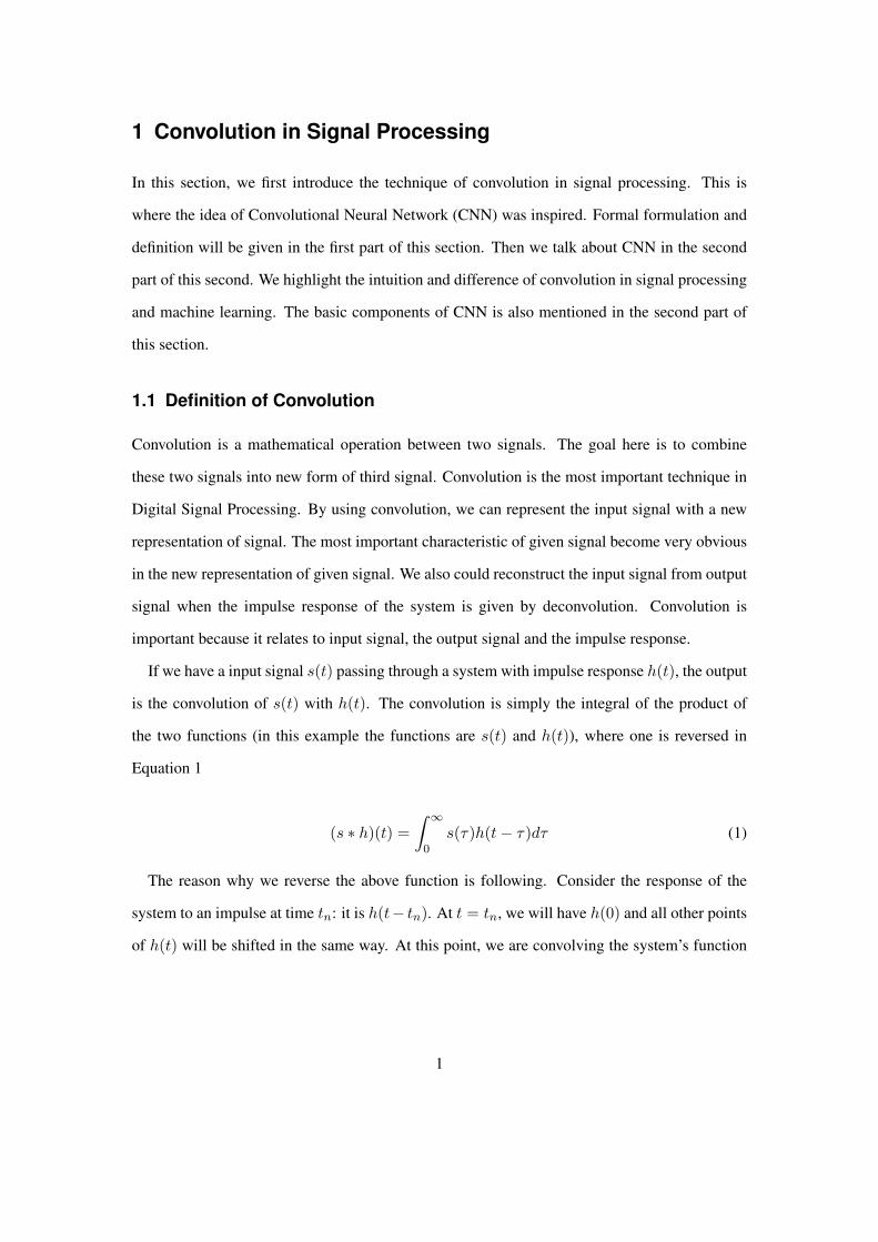
Figure 3: An example of 2D convolution.

Figure 1 shows an example of 2D matrix representation of impulse function h[n]. The shaded

center point is the origin where m = 0 and n = 0.

Once again, a signal can be decomposed into a sum of scaled and shifted impulse functions

h[n]

o[m,n] = s[m,n] ∗ h[m,n] =

∞∑

u=−∞

∞∑

v=−∞s[u, v]h[m− u, n− v] (7)

Notice that the kernel (impulse response) in 2D is center originated in most cases, which

means the center point of a kernel is h[0, 0]. For example, if the kernel size is 5, then the array

index of 5 elements will be -2, -1, 0, 1, and 2. The origin is located at the middle of kernel.

Figure 3 is a simple example of convolution of 3×3 input signal and impulse response (kernel)

in 2D spatial.

In general, the size of output signal is getting bigger than input signal, but we compute only

same area as input has been defined. Because we forced to pad zeros where inputs are not

defined, such as x[−1,−1], the results around the edge cannot be accurate. Plus, the size of

output is fixed as same as input size in most image processing.

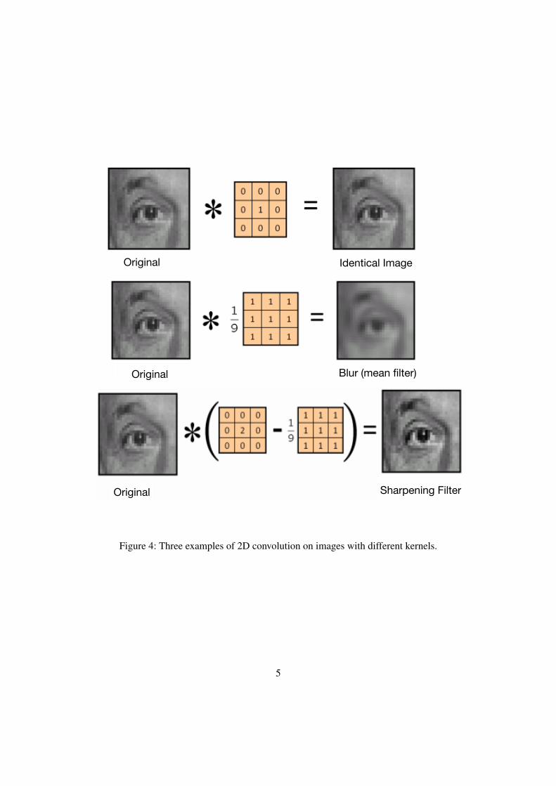
Figure 4 shows three diferent filters operate on the same image. From the results on the

right side we could easily tell the differnce. The first kernel funcion as an identical operation,

which did nothing on original image. The second filter blurs the original image. The last filter

accentuates the edges on the given image.

4

Original

Original

Original

Identical Image

Blur (mean filter)

Sharpening Filter

Figure 4: Three examples of 2D convolution on images with different kernels.

5

2 Basic Compontents of Convolutional Neural Networks

In recent years, deep artificial neural networks (including recurrent ones) have won numerous

contests in pattern recognition and machine learning. Convolutional Neural Networks is one of

the most widely used model of deep learning. In this section, we first introduce the Multiple

Layer Perceptron (MLP) which is the deep model CNN build on. And we discuss the most

important two basic componients of CNN. The application of CNN in both computer vision and

NLP can be viewed as varients of this basic model.

2.1 Multiple Layer Perceptron

In this section, we are going to use one hidden-layer Multi-Layer Perceptron (MLP) for demon-

strating the basic architechture of deep neural networks. An MLP function as a logistic regres-

sion classifier whose input signal is first transformed by a learnt non-linear transformation Φ.

The goal of this non-linear projection is trying to project the data into a new space where the

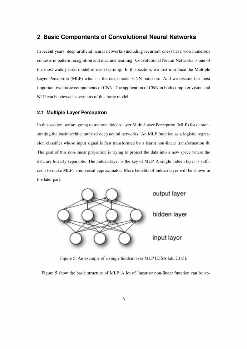
data are linearly separable. The hidden layer is the key of MLP. A single hidden layer is suffi-

cient to make MLPs a universal approximator. More benefits of hidden layer will be shown in

the later part.

Figure 5: An example of a single hidden layer MLP [LISA lab, 2015].

Figure 5 show the basic structure of MLP. A lot of linear or non-linear function can be ap-

6

proach by MLP. For similarity, we only consider the most classical case of a single hidden layer

neural network, mapping a d-vector to an m-vector:

g(x) = b+Wtanh(c+ V x) (8)

where x ∈ Rd is input vector, V ∈ Rk×d is called input to hidden weights, c ∈ Rk is hidden

units offsets or biases, b ∈ Rm is ouput bias or offset, and W ∈ Rm×h is hidden to output

weights.

The vector function h(x) = tanh(c+ V x) is called the output of the hidden layer. Note how

the output is an affine transformation of the hidden layer, in the above network. A non-linearity

may be tacked on to it in some network architectures. The elements of the hidden layer are

called hidden units.

The kind of operation computed by the above h(x) can be applied on h(x) itself, but with

different parameters (different biases and weights). This would give rise to a feedforward multi-

layer network with two hidden layers. More generally, one can build a deep neural network by

stacking more such layers. Each of these layers may have a different dimension (k above). A

common variant is to have skip connections, i.e., a layer can take as input not only the layer at

the previous level but also some of the lower layers.

In order to train the MLP, we first need to do forward propagation of a training pattern’s input

through the neural network in order to generate the propagation’s output activations. When

the forward propagation reaches the last layer, there is a error can be calculated based on the

expected output and real output value.

Backward propagation of the propagation’s output activations through the neural network

using the training pattern target in order to generate the deltas of all output and hidden neurons.

The idea of backward propagation is trying to compute how the error is generated from each

node in each layer. Then we could use gradient decent based method to correct these mistakes

or errors recursively or layer by layer.

7

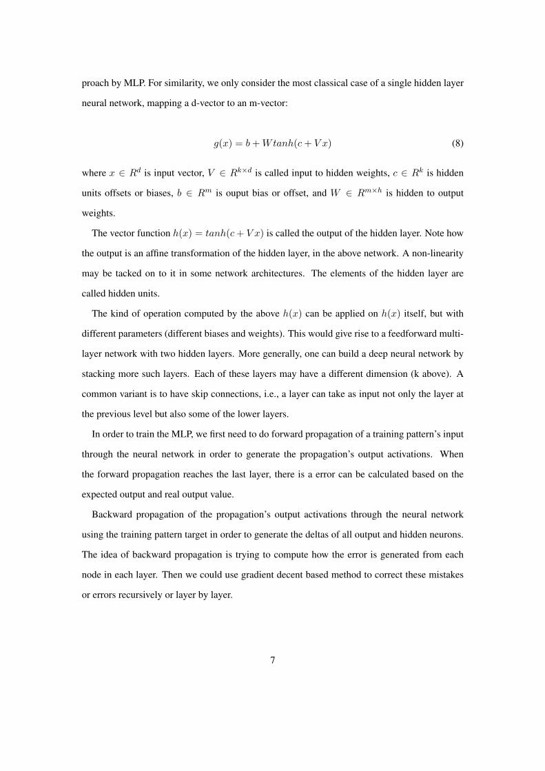
The error function is defined as follows:

E =1

2(t− y)2 (9)

where E is the squared error, t is the target output,

y =n∑

i=1

wihk − 1 (10)

y is the output from forward propagation. n is the number of input units to the neuron.

In order to caculate the error in each layer, we compute the gradient respect to E recursively

at each layer, as show in following:

∂E

∂wi=dE

dy

dy

dnet

∂net

∂wi(11)

In above equation, ∂E∂wi

represents how the error changes when the weights are changed. dEdy

represents how the error changes when the output is changed. dydnet represents how the output

changes when the weighted sum changes. ∂net∂wi

represents how the weighted sum changes as the

weights change.

Then we could update the weight wi by the following equation:

∆wi = α(t− y)xi (12)

where ∆wi is the amount of updated we will make for each layer, α represents the learning rate.

There are several hyper-parameters in the above code, which are not optimized by gradient

descent. Strictly speaking, finding an optimal set of values for these hyper-parameters is not a

feasible problem. First, we cant simply optimize each of them independently. Second, we cannot

readily apply gradient techniques that we described previously (partly because some parameters

are discrete values and others are real-valued). Third, the optimization problem is not convex

and finding a (local) minimum would involve a non-trivial amount of work.

8

2.2 Two Important Components of Convolutional Neural Network

The idea of convolution is first applied in signal processing area. But The concepts of Convolu-

tional Neural Networks (CNN) are inspired from biological area. The concepts of visual cortex

receives high attention from Hubel and Wiesels early work on the cats visual cortex [Hubel and

Wiesel, 1968] study. The visual cortex contains a complex arrangement of cells which are sensi-

tive to small sub-regions of visual field. In our visual field, there are many visual cortex are tiled

together to get the global view. Each visual cortex cells functions as local filter over the entire

input feature space to exploit the strong spatial local correlation in natural images.

The model of CNN is different when it was applied to different area such as computer vision

and NLP. However, there are two basic components are still kept: convolution layer and pooling

layer. We will discuss these two components separately in two different sections. The difference

will be highlighted in the section of computer vision and NLP.

2.2.1 Convolution Layer

In each convolutional layer, the convolutional filter exploits the local correlation by enforcing

a local connectivity pattern among adjacent layers. The upper layer m are already get from a

subset of units from lower layer m-1. Comparing with MLP, another advantage of convolutional

layer is the number of parameters are significantly reduced due to the sharing parameters. The

connectivity is illustrated in Figure 6.

Layer m-1 is feature input from retina. In Figure 6, we take the example of receptive fields

with the width of 3 and thus 3 adjacent neurons are connected with the same parameter in the

retina layer (the button layer). For the above layer, the convolutional operation follows the same

process as previous layers. There is one thing we need to note here is, in layer m-1, only three

adjacent neurons are connected. But for upper layer, their receptive field with respect to the

input is larger (5 instead of 3). During the training processing, the filters are learnt to produce

strongest response to a spatially local input pattern. The example in Figure 6 only represent three

layers of convolution. If we stack more and more layers, the filter become increasingly global.

9

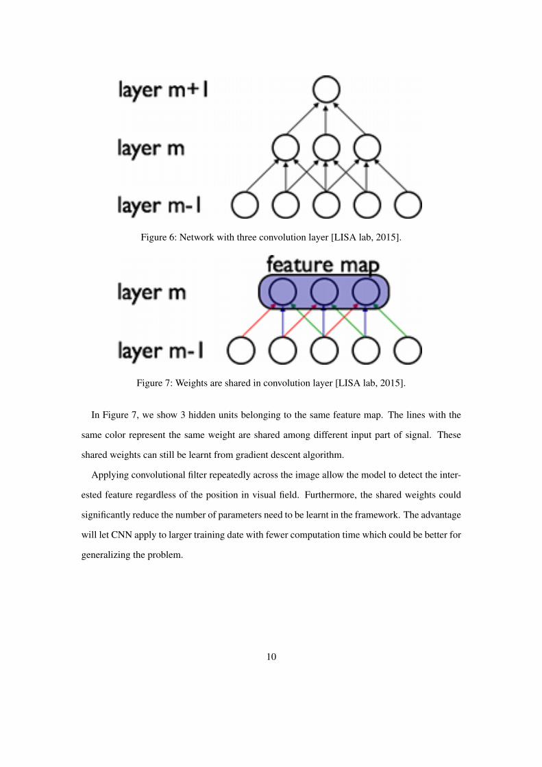
Figure 6: Network with three convolution layer [LISA lab, 2015].

Figure 7: Weights are shared in convolution layer [LISA lab, 2015].

In Figure 7, we show 3 hidden units belonging to the same feature map. The lines with the

same color represent the same weight are shared among different input part of signal. These

shared weights can still be learnt from gradient descent algorithm.

Applying convolutional filter repeatedly across the image allow the model to detect the inter-

ested feature regardless of the position in visual field. Furthermore, the shared weights could

significantly reduce the number of parameters need to be learnt in the framework. The advantage

will let CNN apply to larger training date with fewer computation time which could be better for

generalizing the problem.

10

2.2.2 Pooling Layer

The second important component of CNN is pooling. The pooling layer functions as non-linear

down-sampling. The pooling algorithm only focus on particular sub-region of feature map. The

goal for pooling is trying to the most meaningful information from a particular region.

Pooling algorithm is important for three reasons:

• By eliminating non-maximal values, it reduces computation for upper layers.

• It provides a form of translation invariance. Imagine cascading a max-pooling layer with

a convolutional layer.

• In some case, pooling is helpful for summarizing different feature length into same di-

mension.

3 Convolutional Neural Networks in Computer Vision

CNN is first introduced for solving digits recognition problems [LeCun et al., 1995]. In that digit

recognition task CNN has demonstrated excellent performance. Since then, CNN has received a

great attention in the area of computer vision for many different tasks, such as, face recognition,

object detection, salience detection and so on. There are several reasons for this: (1) CNN could

handle larger training sets due to the weights are shared in convolutional layer; (2) better model

regularization methods are introduced for avoiding over-fitting, such as Dropout [Hinton et al.,

2012]; (3) Larger datasets become available for training, such as ImageNet [Deng et al., 2009];

(4) powerful GPU based convolution implementations, such as CUDA.

In this section, we show the basic structure of CNN in computer vision. We first show the spe-

cial structure of CNN in computer vision application. Then the second part focuses on another

CNN variation, Deconvolutional Neural Network.

11

3.1 Multiple Level of Convolution and Pooling

As we mentioned in 2, CNN model has two basic components: convolutional layer and max-

pooling. The first process for CNN in computer vision problem is apply convolutional kernel

repeatedly across sub-regions of the entire image. From mathematical point of view, this process

operates the convolutional processes with a fixed filter over image. In order to chapter enough

non-linearity of the input signal, in most cases, we will apply a non-linear function, such as

tanh, over the convolution results. We denote the the kth feature map at a given layer as hk. The

feature map, hk, is determined by the weights W k and bias bk. Equation 14 formally defined

how the feature map, hk is calculated with non-linear activation function tanh.

hkij = tanh(bk + (W k ∗ x)i,j) (13)

The above equation is only for the feature map which is obtained by one filter. However,

one filter only can capture one particular signal pattern. In order to capture enough variance

of data patterns, only one filter is far from enough. Therefore, in order to form a richer rep-

resentation of the in put signal, in most cases, we will use multiple filters (e.g. 100). Since

multiple convolutional filter is employed, each hidden layer is composed of multiple feature

maps, {h(k), k = 0..K}. A 4D tensor containing elements for every combination of destination

feature map, source feature map, input image’s vertical and horizontal position is represented

as W. The biases b can be represented as a vector containing one element for every destination

feature map. The idea of the convolutional layer is shown in Figure 16

Figure 16 shows two layers of a CNN. There are four feature maps in the layer m − 1. And

two feature maps (h0 and h1) in hidden layer m. Different color in layer m− 1 represents four

different feature maps in layer m− 1. We first apply one 2× 2 convolutional filter upon the four

feature maps in m − 1 layer, then we save the result in the first feature map in layer m. Then

the second convolutional filter is apply with the same process, and we get the second feature

map in the layer m. We call the 2× 2 convolutional filter in layer m− 1 as receptive field. The

12

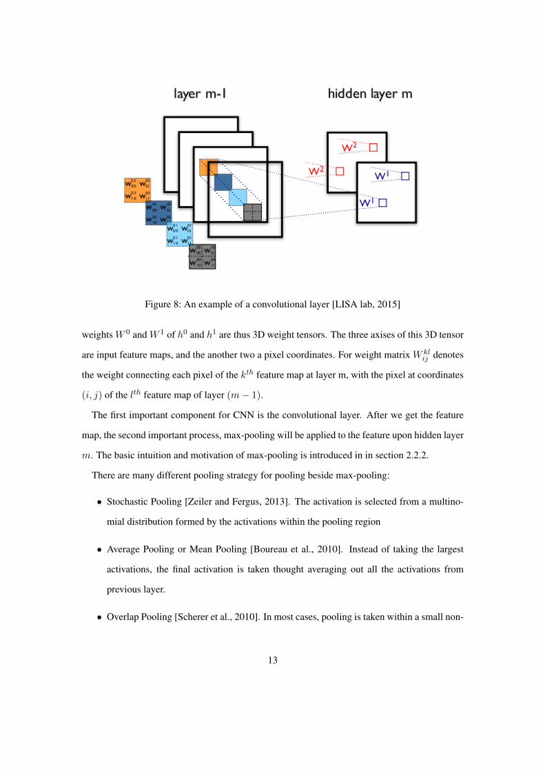
Figure 8: An example of a convolutional layer [LISA lab, 2015]

weights W 0 and W 1 of h0 and h1 are thus 3D weight tensors. The three axises of this 3D tensor

are input feature maps, and the another two a pixel coordinates. For weight matrix W klij denotes

the weight connecting each pixel of the kth feature map at layer m, with the pixel at coordinates

(i, j) of the lth feature map of layer (m− 1).

The first important component for CNN is the convolutional layer. After we get the feature

map, the second important process, max-pooling will be applied to the feature upon hidden layer

m. The basic intuition and motivation of max-pooling is introduced in in section 2.2.2.

There are many different pooling strategy for pooling beside max-pooling:

• Stochastic Pooling [Zeiler and Fergus, 2013]. The activation is selected from a multino-

mial distribution formed by the activations within the pooling region

• Average Pooling or Mean Pooling [Boureau et al., 2010]. Instead of taking the largest

activations, the final activation is taken thought averaging out all the activations from

previous layer.

• Overlap Pooling [Scherer et al., 2010]. In most cases, pooling is taken within a small non-

13

Figure 9: Pipeline of CNN for computer vision tasks [LISA lab, 2015].

overlapping receptive field of the previous layer. Overlap pooling is taken over a serious

of overlapped areas.

The above discussion only include one convolution layer and one pooling layer. However, in

most computer vision tasks, there are multiple convolutional layers and pooling layer. Figure 9

show a pipeline of CNN for computer vision tasks. As we discuss in section 2, convolutional

layer only capture the information from one small region of given image. In order to get global

view of given image, multiple level of convolutional layers and pooling layers are usually used.

Convolutional layers and max-pooling are at the heart of the LeNet family of models. After

multiple step of convolution and pooling, the final representation of given image are feed into a

traditional MLP for classification purpose.

3.2 Deconvolutional Networks for Decoding Purpose

CNN is a type of feed-forward network that trying to encode the input image’s information into

a final representation. In this encoding process, many feature detectors spatially pool edge in-

formation which destroys cues such as edge intersections, parallelism and symmetry. In kind of

encoding frameworks serves well for classification problems in computer vision tasks. However,

there are also some computer vision tasks are dealing with corrupted images.

Deconvolutional Networks [Zeiler et al., 2010] are introduced to solve these problems. CNN

is a bottom-up framework whose input signal is subjected to multiple layers of convolutionss,

nonlinearities and sub-sampling. Comparing with CNN, Deconvolutional Networks are top-

14

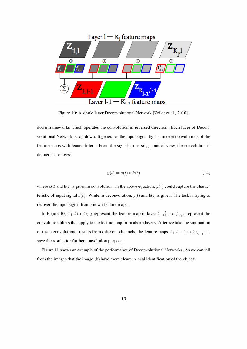
Figure 10: A single layer Deconvolutional Network [Zeiler et al., 2010].

down frameworks which operates the convolution in reversed direction. Each layer of Decon-

volutional Network is top-down. It generates the input signal by a sum over convolutions of the

feature maps with leaned filters. From the signal processing point of view, the convolution is

defined as follows:

y(t) = s(t) ∗ h(t) (14)

where s(t) and h(t) is given in convolution. In the above equation, y(t) could capture the charac-

teristic of input signal s(t). While in deconvolution, y(t) and h(t) is given. The task is trying to

recover the input signal from known feature maps.

In Figure 10, Z1, l to ZK1,l represent the feature map in layer l. f l1,1 to f lKi,1represent the

convolution filters that apply to the feature map from above layers. After we take the summation

of these convolutional results from different channels, the feature maps Z1, l − 1 to ZKl−1,l−1

save the results for further convolution purpose.

Figure 11 shows an example of the performance of Deconvolutional Networks. As we can tell

from the images that the image (b) have more clearer visual identification of the objects.

15

(a) Original Image (b) Image after Deconvolutional Net-work

Figure 11: Deconvolutional Networks performance [Xu et al., 2014]

4 Convolutional Neural Networks in Natural Language

Processing

Convolutional neural networks (CNNs), originally invented in computer vision [LeCun et al.,

1995], has recently attracted much attention in natural language processing (NLP) on problems

such as sequence labeling [Collobert et al., 2011], semantic parsing [Yih et al., 2014], and search

query retrieval [Shen et al., 2014]. In particular, recent work on CNN-based sentence modeling

[Kalchbrenner et al., 2014, Kim, 2014] has achieved excellent, often state-of-the-art, results on

various classification tasks such as sentiment, subjectivity, and question-type classification.

The first section of covers several techniques that use CNN as an encoding method for sen-

tence modeling. The first method is simply applied CNN framework from computer vision to

NLP task. The second method acheives better performance by using more NLP domain specific

knowledges such as linguistics infomation and sentence structure information. The second part

of this section introduce several techniques that employ CNN as encoding model for Machine

Translation.

16

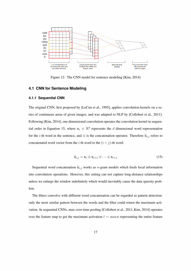
Figure 12: The CNN model for sentence modeling [Kim, 2014]

4.1 CNN for Sentence Modeling

4.1.1 Sequential CNN

The original CNN, first proposed by [LeCun et al., 1995], applies convolution kernels on a se-

ries of continuous areas of given images, and was adapted to NLP by [Collobert et al., 2011].

Following [Kim, 2014], one dimensional convolution operates the convolution kernel in sequen-

tial order in Equation 15, where xi ∈ Rd represents the d dimensional word representation

for the i-th word in the sentence, and ⊕ is the concatenation operator. Therefore xi,j refers to

concatenated word vector from the i-th word to the (i+ j)-th word:

xi,j = xi ⊕ xi+1 ⊕ · · · ⊕ xi+j (15)

Sequential word concatenation xi,j works as n-gram models which feeds local information

into convolution operations. However, this setting can not capture long-distance relationships

unless we enlarge the window indefinitely which would inevitably cause the data sparsity prob-

lem.

The filters convolve with different word concatenation can be regarded as pattern detection:

only the most similar pattern between the words and the filter could return the maximum acti-

vation. In sequential CNNs, max-over-time pooling [Collobert et al., 2011,Kim, 2014] operates

over the feature map to get the maximum activation c = max c representing the entire feature

17

Despite the film ’s shortcomings the stories are quietly moving .

ROOT

Figure 1: Running example from Movie Reviews dataset.

mensional word representation for the i-th word inthe sentence, and ⊕ is the concatenation operator.Therefore xi,j refers to concatenated word vectorfrom the i-th word to the (i+ j)-th word:

xi,j = xi ⊕ xi+1 ⊕ · · · ⊕ xi+j (1)

Sequential word concatenation xi,j works asn-gram models which feeds local information intoconvolution operations. However, this setting cannot capture long-distance relationships unless weenlarge the window indefinitely which would in-evitably cause the data sparsity problem.

In order to capture the long-distance dependen-cies we propose the dependency tree-based con-volution model (DTCNN). Figure 1 illustrates anexample from the Movie Reviews (MR) dataset(Pang and Lee, 2005). The sentiment of this sen-tence is obviously positive, but this is quite dif-ficult for sequential CNNs because many n-gramwindows would include the highly negative word“shortcomings”, and the distance between “De-spite” and “shortcomings” is quite long. DTCNN,however, could capture the tree-based bigram“Despite – shortcomings”, thus flipping the senti-ment, and the tree-based trigram “ROOT – moving– stories”, which is highly positive.

2.1 Convolution on Ancestor PathsWe define our concatenation based on the depen-dency tree for a given modifier xi:

xi,k = xi ⊕ xp(i) ⊕ · · · ⊕ xpk−1(i) (2)

where function pk(i) returns the i-th word’s k-thancestor index, which is recursively defined as:

pk(i) =

{p(pk−1(i)) if k > 0

i if k = 0(3)

Figure 2 (left) illustrates ancestor paths patternswith various orders. We always start the convo-lution with xi and concatenate with its ancestors.If the root node is reached, we add “ROOT” asdummy ancestors (vertical padding).

For a given tree-based concatenated word se-quence xi,k, the convolution operation applies afilter w ∈ Rk×d to xi,k with a bias term b de-scribed in equation 4:

ci = f(w · xi,k + b) (4)

where f is a non-linear activation function such asrectified linear unit (ReLu) or sigmoid function.The filter w is applied to each word in the sen-tence, generating the feature map c ∈ Rl:

c = [c1, c2, · · · , cl] (5)where l is the length of the sentence.

2.2 Max-Over-Tree Pooling and DropoutThe filters convolve with different word concate-nation in Eq. 4 can be regarded as pattern detec-tion: only the most similar pattern between thewords and the filter could return the maximum ac-tivation. In sequential CNNs, max-over-time pool-ing (Collobert et al., 2011; Kim, 2014) operatesover the feature map to get the maximum acti-vation c = max c representing the entire featuremap. Our DTCNNs also pool the maximum ac-tivation from feature map to detect the strongestactivation over the whole tree (i.e., over the wholesentence). Since the tree no longer defines a se-quential “time” direction, we refer to our poolingas “max-over-tree” pooling.

In order to capture enough variations, we ran-domly initialize the set of filters to detect differentstructure patterns. Each filter’s height is the num-ber of words considered and the width is alwaysequal to the dimensionality d of word representa-tion. Each filter will be represented by only onefeature after max-over-tree pooling. After a seriesof convolution with different filter with differentheights, multiple features carry different structuralinformation become the final representation of theinput sentence. Then, this sentence representationis passed to a fully connected soft-max layer andoutputs a distribution over different labels.

Neural networks often suffer from overtrain-ing. Following Kim (2014), we employ randomdropout on penultimate layer (Hinton et al., 2012).in order to prevent co-adaptation of hidden units.In our experiments, we set our drop out rate as 0.5and learning rate as 0.95 by default. FollowingKim (2014), training is done through stochasticgradient descent over shuffled mini-batches withthe Adadelta update rule (Zeiler, 2012).

2.3 Convolution on SiblingsAncestor paths alone is not enough to capturemany linguistic phenomena such as conjunction.

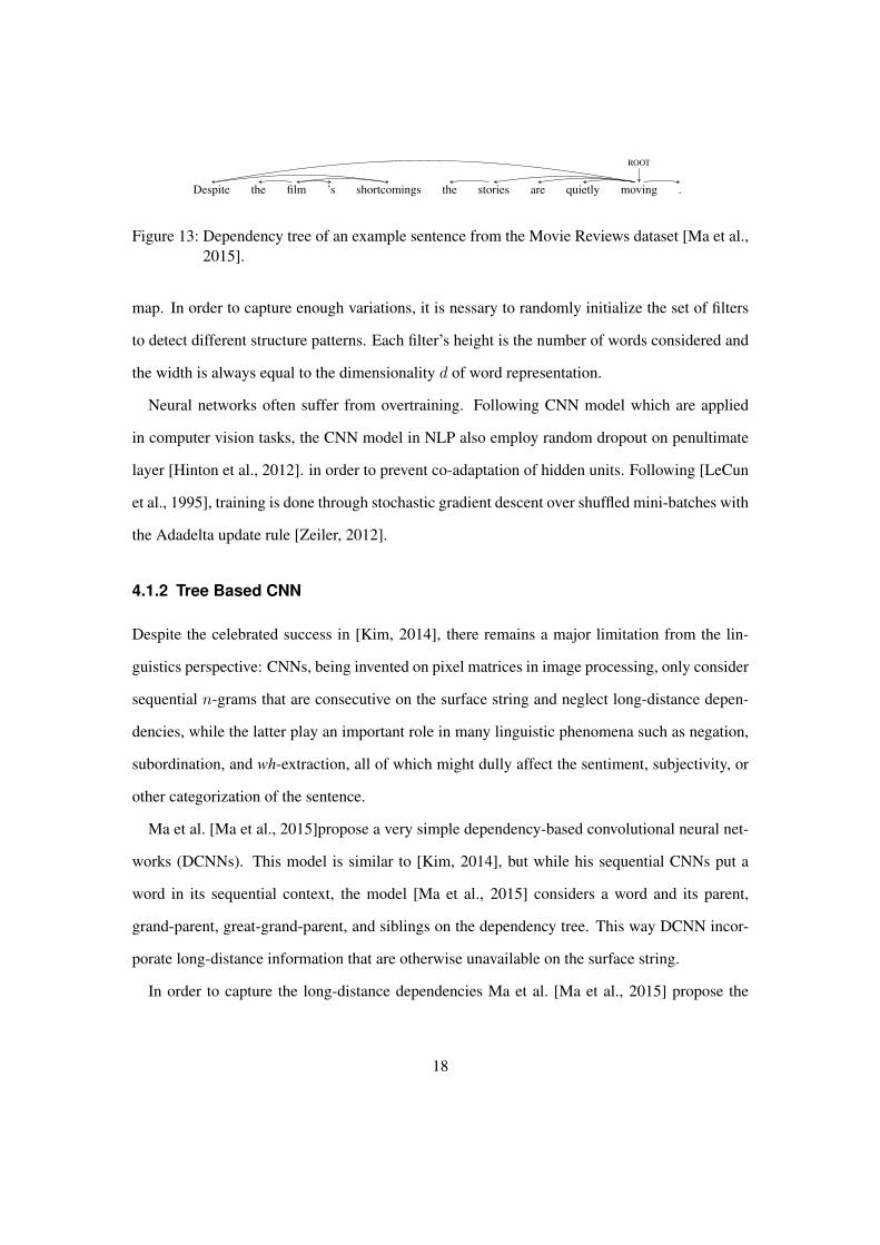
Figure 13: Dependency tree of an example sentence from the Movie Reviews dataset [Ma et al.,2015].

map. In order to capture enough variations, it is nessary to randomly initialize the set of filters

to detect different structure patterns. Each filter’s height is the number of words considered and

the width is always equal to the dimensionality d of word representation.

Neural networks often suffer from overtraining. Following CNN model which are applied

in computer vision tasks, the CNN model in NLP also employ random dropout on penultimate

layer [Hinton et al., 2012]. in order to prevent co-adaptation of hidden units. Following [LeCun

et al., 1995], training is done through stochastic gradient descent over shuffled mini-batches with

the Adadelta update rule [Zeiler, 2012].

4.1.2 Tree Based CNN

Despite the celebrated success in [Kim, 2014], there remains a major limitation from the lin-

guistics perspective: CNNs, being invented on pixel matrices in image processing, only consider

sequential n-grams that are consecutive on the surface string and neglect long-distance depen-

dencies, while the latter play an important role in many linguistic phenomena such as negation,

subordination, and wh-extraction, all of which might dully affect the sentiment, subjectivity, or

other categorization of the sentence.

Ma et al. [Ma et al., 2015]propose a very simple dependency-based convolutional neural net-

works (DCNNs). This model is similar to [Kim, 2014], but while his sequential CNNs put a

word in its sequential context, the model [Ma et al., 2015] considers a word and its parent,

grand-parent, great-grand-parent, and siblings on the dependency tree. This way DCNN incor-

porate long-distance information that are otherwise unavailable on the surface string.

In order to capture the long-distance dependencies Ma et al. [Ma et al., 2015] propose the

18

ancestor paths siblingsn pattern(s) n pattern(s)

3m h g

2s m

4m h g g2

3s m h t s m

5m h g g2 g3

4t s m h s m h g

Table 1: Tree-based convolution patterns. Word concatenation always starts with m, while h, g, and g2

denote parent, grand parent, and great-grand parent, etc., and “ ” denotes words excluded in convolution.

2.3 Convolution on SiblingsAncestor paths alone is not enough to capturemany linguistic phenomena such as conjunction.Inspired by higher-order dependency parsing (Mc-Donald and Pereira, 2006; Koo and Collins, 2010),we also incorporate siblings for a given word invarious ways. See Table 1 (right) for details.

2.4 Combined ModelPowerful as it is, structural information still doesnot fully cover sequential information. Also, pars-ing errors (which are common especially for in-formal text such as online reviews) directly affectDTCNN performance while sequential n-gramsare always correctly observed. To best exploitboth information, we want to combine both mod-els. The easiest way of combination is to con-catenate these representations together, then feedinto fully connected soft-max neural networks. Inthese cases, combine with different feature fromdifferent type of sources could stabilize the perfor-mance. The final sentence representation is thus:

c = [c(1)a , ..., c(Na)a︸ ︷︷ ︸

ancestors

; c(1)s , ..., c(Ns)s︸ ︷︷ ︸

siblings

; c(1), ..., c(N)

︸ ︷︷ ︸sequential

]

where Na, Ns, and N are the number of ancestor,sibling, and sequential filters. In practice, we use100 filters for each template in Table 1. The fullycombined representation is 1100-dimensional bycontrast to 300-dimensional for sequential CNN.

3 ExperimentsWe implement our DTCNN on top of the opensource CNN code by Kim (2014).1 Table 2summarizes our results in the context of otherhigh-performing efforts in the literature. We usethree benchmark datasets in two categories: senti-ment analysis on both Movie Review (MR) (Pangand Lee, 2005) and Stanford Sentiment Treebank

1https://github.com/yoonkim/CNN sentence

(SST-1) (Socher et al., 2013) datasets, and ques-tion classification on TREC (Li and Roth, 2002).

For all datasets, we first obtain the dependencyparse tree from Stanford parser (Manning et al.,2014).2 Different window size for different choiceof convolution are shown in Table 1. For thedataset without a development set (MR), we ran-domly choose 10% of the training data to indicateearly stopping. In order to have a fare compari-son with baseline CNN, we also use 3 to 5 as ourwindow size. Most of our results are generatedby GPU due to its efficiency, however CPU poten-tially could generate better results.3 Our imple-mentation can be found on Github.4

3.1 Sentiment AnalysisBoth sentiment analysis datasets (MR and SST-1) are based on movie reviews. The differencesbetween them are mainly in the different num-bers of categories and whether the standard splitis given. There are 10,662 sentences in the MRdataset. Each instance is labeled positive or neg-ative, and in most cases contains one sentence.Since no standard data split is given, following theliterature we use 10 fold cross validation to includeevery sentence in training and testing at least once.Concatenating with sibling and sequential infor-mation obviously improves tree-based CNNs, andthe final model outperforms the baseline sequen-tial CNNs by 0.4, and ties with Zhu et al. (2015).

Different from MR, the Stanford SentimentTreebank (SST-1) annotates finer-grained labels,very positive, positive, neutral, negative and verynegative, on an extension of the MR dataset. Thereare 11,855 sentences with standard split. Ourmodel achieves an accuracy of 49.5 which is sec-ond only to Irsoy and Cardie (2014). We set batchsize to 100 for this task.

2The phrase-structure trees in SST-1 are actually automat-ically parsed, and thus can not be used as gold-standard trees.

3GPU only supports float32 while CPU supports float64.4https://github.com/cosmmb/DTCNN

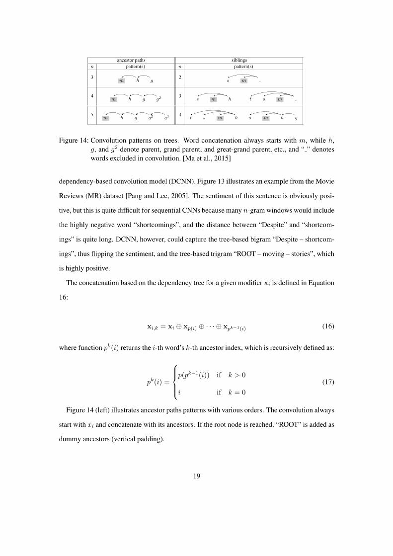
Figure 14: Convolution patterns on trees. Word concatenation always starts with m, while h,g, and g2 denote parent, grand parent, and great-grand parent, etc., and “ ” denoteswords excluded in convolution. [Ma et al., 2015]

dependency-based convolution model (DCNN). Figure 13 illustrates an example from the Movie

Reviews (MR) dataset [Pang and Lee, 2005]. The sentiment of this sentence is obviously posi-

tive, but this is quite difficult for sequential CNNs because many n-gram windows would include

the highly negative word “shortcomings”, and the distance between “Despite” and “shortcom-

ings” is quite long. DCNN, however, could capture the tree-based bigram “Despite – shortcom-

ings”, thus flipping the sentiment, and the tree-based trigram “ROOT – moving – stories”, which

is highly positive.

The concatenation based on the dependency tree for a given modifier xi is defined in Equation

16:

xi,k = xi ⊕ xp(i) ⊕ · · · ⊕ xpk−1(i) (16)

where function pk(i) returns the i-th word’s k-th ancestor index, which is recursively defined as:

pk(i) =

p(pk−1(i)) if k > 0

i if k = 0

(17)

Figure 14 (left) illustrates ancestor paths patterns with various orders. The convolution always

start with xi and concatenate with its ancestors. If the root node is reached, “ROOT” is added as

dummy ancestors (vertical padding).

19

Category Model MR SST-1 TREC TREC-2

This workDCNNs: ancestor 80.4† 47.7† 95.4† 88.4†

DCNNs: ancestor+sibling 81.7† 48.3† 95.6† 89.0†

DCNNs: ancestor+sibling+sequential 81.9 49.5 95.4† 88.8†

CNNsCNNs-non-static [Kim, 2014] – baseline 81.5 48.0 93.6 86.4∗

CNNs-multichannel [Kim, 2014] 81.1 47.4 92.2 86.0∗

Deep CNNs [Kalchbrenner et al., 2014] - 48.5 93.0 -

Recursive NNsRecursive Autoencoder [Socher et al., 2011] 77.7 43.2 - -Recursive Neural Tensor [Socher et al., 2013] - 45.7 - -Deep Recursive NNs [Irsoy and Cardie, 2014] - 49.8 - -

Recurrent NNs LSTM on tree [Zhu et al., 2015] 81.9 48.0 - -Other deep learning Paragraph-Vec [Le and Mikolov, 2014] - 48.7 - -Hand-coded rules SVMS [Silva et al., 2011] - 95.0 90.8

Table 1: Results on Movie Review (MR), Stanford Sentiment Treebank (SST-1), and TRECdatasets. TREC-2 is TREC with fine grained labels. †Results generated by GPU (allothers generated by CPU). ∗Results generated from [Kim, 2014]’s implementation. [Maet al., 2015]

For a given tree-based concatenated word sequence xi,k, the convolution operation applies a

filter w ∈ Rk×d to xi,k with a bias term b described in equation 18:

ci = f(w · xi,k + b) (18)

where f is a non-linear activation function such as rectified linear unit (ReLu) or sigmoid func-

tion. The filter w is applied to each word in the sentence, generating the feature map c ∈ Rl:

c = [c1, c2, · · · , cl] (19)

where l is the length of the sentence.

DCNNs also pool the maximum activation from feature map to detect the strongest activation

over the whole tree (i.e., over the whole sentence). Since the tree no longer defines a sequential

“time” direction, the pooling for tree-based convolution are referred as “max-over-tree” pooling.

Table 1 summarizes results for both sequential based and tree based convolution results. As

we can tell from the results. Tree based convolution acheives better result accross all the tasks.

Figure 15 visualizes examples where CNN errs while DCNN does not. For example, CNN

20

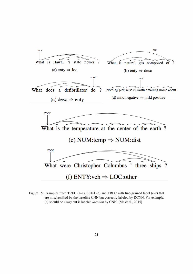
Figure 15: Examples from TREC (a–c), SST-1 (d) and TREC with fine-grained label (e–f) thatare misclassified by the baseline CNN but correctly labeled by DCNN. For example,(a) should be entity but is labeled location by CNN. [Ma et al., 2015]

21

labels (a) as location due to “Hawaii” and “state”, while the long-distance backbone “What –

flower” is clearly asking for an entity. Similarly, in (d), DCNN captures the obviously negative

tree-based trigram “Nothing – worth – emailing”. Note that DCNN model also works with non-

projective dependency trees such as the one in (b). The last two examples in Figure 15 visualize

cases where DCNN outperforms the baseline CNNs in fine-grained TREC. In example (e), the

word “temperature” is at second from the top and is root of a 8 word span “the ... earth”. When

DCNN use a window of size 5 for tree convolution, every words in that span get convolved with

“temperature” and this should be the reason why DCNN get correct.

4.2 CNN for Machine Translation

Most machine translation technique are statical based approach. The basic component of trans-

lation systems need to estimate translation probabilities for pairs of phrases. One phrase comes

from source side and the another comes from target side. Such model need to count the occur-

rences of the phrase pairs. Although distinct phrase pairs share significant similarities, they do

not share statistical weight in the model’s estimation of their translation probabilities. There-

fore, it is intuitive helpful if we could use continuous representations for the phrase pair. CNN

demonstrates a powerful ability for sentence modeling. Based on this successful sentence en-

coding ability, CNN is also can be served as powerful technique for Machine Translation tasks

due to the continuous representation from word embedding.

The first CNN based machine translation model is proposed with the name of Recurrent

Continuous Translation Models (RCTM) [Kalchbrenner and Blunsom, 2013]. RCTM map the

source language to a probability distribution over the sentence in the target language without

losing generality. In this model, they use CNN as an encoding method and use Recurrent Neural

Network for decoding or generating the target sentence.

Figure 16 is the encoding framework for RCTM. Ee represents the sentence matrix from

source side. K2 to K3 are the filters for different convolutional layers. L3 represents the weight

matrix that merge the previous convolutional results into a final representation e.The encoding

22

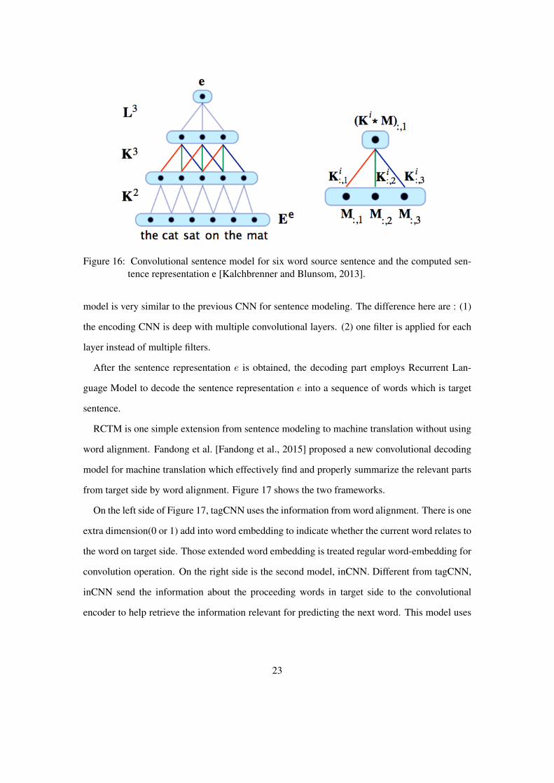
Figure 16: Convolutional sentence model for six word source sentence and the computed sen-tence representation e [Kalchbrenner and Blunsom, 2013].

model is very similar to the previous CNN for sentence modeling. The difference here are : (1)

the encoding CNN is deep with multiple convolutional layers. (2) one filter is applied for each

layer instead of multiple filters.

After the sentence representation e is obtained, the decoding part employs Recurrent Lan-

guage Model to decode the sentence representation e into a sequence of words which is target

sentence.

RCTM is one simple extension from sentence modeling to machine translation without using

word alignment. Fandong et al. [Fandong et al., 2015] proposed a new convolutional decoding

model for machine translation which effectively find and properly summarize the relevant parts

from target side by word alignment. Figure 17 shows the two frameworks.

On the left side of Figure 17, tagCNN uses the information from word alignment. There is one

extra dimension(0 or 1) add into word embedding to indicate whether the current word relates to

the word on target side. Those extended word embedding is treated regular word-embedding for

convolution operation. On the right side is the second model, inCNN. Different from tagCNN,

inCNN send the information about the proceeding words in target side to the convolutional

encoder to help retrieve the information relevant for predicting the next word. This model uses

23

Figure 17: Joint language model based on CNN encoder [Fandong et al., 2015].

the information from preceeding word, h(e2, e3, e4) to injected into every convolution window

in the source language sentence. In this model, inCNN provides complementary information in

the augmented joint language model of taqCNN. The results of both model is shown in Figure

18.

Figure 18: BLEU score on NIST MT04 and MT05 [Fandong et al., 2015].

24

5 Conclusion

In this survey, we first show the intuition and definition of convolution in signal processing.

Then we show how the convolution is used in machine learning area. Two important components

of CNN are highlighted: convolution layer and max-pooling. In the applications of computer

vision, we show the details of how the convolution layer and max-pooling are used. Another

variation of CNN, Deconvolutional Network is also covered. We also show how CNN is adapted

into NLP problems such like sentence modeling and machine translation. The details of the how

the CNN is adapted into NLP problem is also discussed.

25

References

Boureau, Y.-L., Ponce, J., and Lecun, Y. (2010). A theoretical analysis of feature pooling in vi-

sual recognition. In 27TH INTERNATIONAL CONFERENCE ON MACHINE LEARNING,

HAIFA, ISRAEL.

Collobert, R., Weston, J., Bottou, L., Karlen, M., Kavukcuoglu, K., and Kuksa, P. (2011). Natu-

ral language processing (almost) from scratch. volume 12, pages 2493–2537.

Deng, J., Dong, W., Socher, R., Li, L.-J., Li, K., and Fei-Fei, L. (2009). ImageNet: A Large-

Scale Hierarchical Image Database. In CVPR09.

Fandong, M., Zhengdong, L., Mingbxuan, W., Hang, l., Wenbin, J., and Qun, L. (2015). Encod-

ing source language with convolutional neural network for machine translation. Beijing.

Hinton, G. E., Srivastava, N., Krizhevsky, A., Sutskever, I., and Salakhutdinov, R. (2012).

Improving neural networks by preventing co-adaptation of feature detectors. volume

abs/1207.0580.

Hubel, D. H. and Wiesel, T. N. (1968). Receptive fields and functional architecture of monkey

striate cortex. Journal of Physiology (London), 195:215–243.

Irsoy, O. and Cardie, C. (2014). Deep recursive neural networks for compositionality in lan-

guage. In Advances in Neural Information Processing Systems, pages 2096–2104.

Kalchbrenner, N. and Blunsom, P. (2013). Recurrent continuous translation models. Seattle.

Association for Computational Linguistics.

Kalchbrenner, N., Grefenstette, E., and Blunsom, P. (2014). A convolutional neural network

for modelling sentences. In Proceedings of the 52nd Annual Meeting of the Association for

Computational Linguistics (Volume 1: Long Papers), pages 655–665, Baltimore, Maryland.

Association for Computational Linguistics.

26

Kim, Y. (2014). Convolutional neural networks for sentence classification. In Proceedings of the

2014 Conference on Empirical Methods in Natural Language Processing (EMNLP), pages

1746–1751, Doha, Qatar. Association for Computational Linguistics.

Le, Q. V. and Mikolov, T. (2014). Distributed representations of sentences and documents.

LeCun, Y., Jackel, L., Bottou, L., Brunot, A., Cortes, C., Denker, J., Drucker, H., Guyon, I.,

Mller, U., Sckinger, E., Simard, P., and Vapnik, V. (1995). Comparison of learning algo-

rithms for handwritten digit recognition. In INTERNATIONAL CONFERENCE ON ARTI-

FICIAL NEURAL NETWORKS, pages 53–60.

LISA lab, U. o. M. (2015). Deep learning tutorial.

Ma, M., Huang, L., Zhou, B., and Xiang, B. (2015). Tree-based convolution for sentence mod-

eling.

Pang, B. and Lee, L. (2005). Seeing stars: Exploiting class relationships for sentiment catego-

rization with respect to rating scales. In Proceedings of ACL, pages 115–124.

Scherer, D., Muller, A., and Behnke, S. (2010). Evaluation of pooling operations in convolu-

tional architectures for object recognition. In Proceedings of the 20th International Confer-

ence on Artificial Neural Networks: Part III, ICANN’10, pages 92–101, Berlin, Heidelberg.

Springer-Verlag.

Shen, Y., he, X., Gao, J., Deng, L., and Mesnil, G. (2014). Learning semantic representations

using convolutional neural networks for web search. WWW 2014.

Silva, J., Coheur, L., Mendes, A. C., and Wichert, A. (2011). From symbolic to sub-symbolic

information in question classification. Artificial Intelligence Review, 35.

Socher, R., Pennington, J., Huang, E. H., Ng, A. Y., and Manning, C. D. (2011). Semi-

Supervised Recursive Autoencoders for Predicting Sentiment Distributions. In Proceedings

of the 2011 Conference on Empirical Methods in Natural Language Processing (EMNLP).

27

Socher, R., Perelygin, A., Wu, J., Chuang, J., Manning, C. D., Ng, A. Y., and Potts, C. (2013).

Recursive deep models for semantic compositionality over a sentiment treebank. In Pro-

ceedings of the 2013 Conference on Empirical Methods in Natural Language Processing,

pages 1631–1642, Stroudsburg, PA. Association for Computational Linguistics.

Xu, L., Ren, J. S., Liu, C., and Jia, J. (2014). Deep convolutional neural network for image

deconvolution. In Ghahramani, Z., Welling, M., Cortes, C., Lawrence, N., and Weinberger,

K., editors, Advances in Neural Information Processing Systems 27, pages 1790–1798.

Curran Associates, Inc.

Yih, W.-t., He, X., and Meek, C. (2014). Semantic parsing for single-relation question answer-

ing. In Proceedings of the 52nd Annual Meeting of the Association for Computational

Linguistics (Volume 2: Short Papers), pages 643–648. Association for Computational Lin-

guistics.

Zeiler, M. (2012). Adadelta: An adaptive learning rate method. Unpublished manuscript:

http://arxiv.org/abs/1212.5701.

Zeiler, M. D. and Fergus, R. (2013). Stochastic pooling for regularization of deep convolutional

neural networks. CoRR, abs/1301.3557.

Zeiler, M. D., Krishnan, D., Taylor, G. W., and Fergus, R. (2010). Deconvolutional networks. In

In CVPR.

Zhu, X., Sobhani, P., and Guo, H. (2015). Long short-term memory over tree structures.

28