Convex Optimization M2 - École Normale Supérieureaspremon/PDF/MVA/FirstOrderMethods.pdf · Convex...

Convex Optimization M2

Lecture 6

A. d’Aspremont. Convex Optimization M2. 1/30

Large Scale Optimization


Outline

� First-order methods: introduction

� Exploiting structure

� First order algorithms

◦ Subgradient methods

◦ Gradient methods

◦ Accelerated gradient methods

� Other algorithms

◦ Coordinate descent methods

◦ Localization methods

◦ Franke-Wolfe

◦ Dykstra, alternating projection

◦ Stochastic optimization


First-order methods: introduction

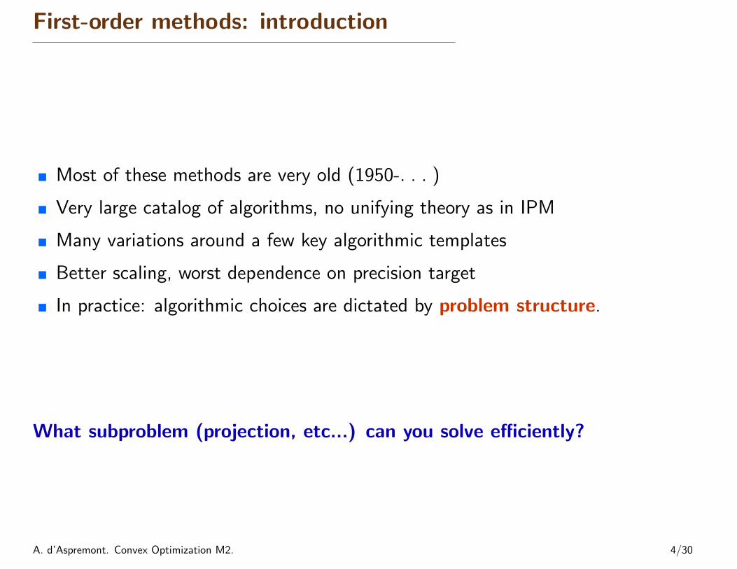
� Most of these methods are very old (1950-. . . )

� Very large catalog of algorithms, no unifying theory as in IPM

� Many variations around a few key algorithmic templates

� Better scaling, worst dependence on precision target

� In practice: algorithmic choices are dictated by problem structure.

What subproblem (projection, etc...) can you solve efficiently?


First Order Algorithms



minimize f(x)subject to x ∈ C

In theory:

� The theoretical convergence speed of gradient based methods is mostlycontrolled by the smoothness of the objective.

� Obviously, the geometry of the (convex) feasible set also has an impact.

Convex objective f(x) Iterations. . .Nondifferentiable O(1/ε2)Differentiable O(1/ε2)Smooth (Lipschitz gradient) O(1/

√ε)

Strongly convex O(log(1/ε))

In practice:

� Compared to IPM, much larger gap between theoretical complexity guaranteesand empirical performance.

� Conditioning, well-posedness, etc. also have a very strong impact.



Solveminimize f(x)subject to x ∈ C

in x ∈ Rn, with C ⊂ Rn convex.

Main assumptions in the subgradient/gradient methods that follow:

� The gradient ∇f(x) or a subgradient can be computed efficiently.

� If C is not Rn, for any y ∈ Rn, the following subproblem can be solvedefficiently

minimize yTx+ d(x)subject to x ∈ C

in the variable x ∈ Rn, where d(x) is a strongly convex function.

Typically, d(x) = ‖x‖2 and this is an Euclidean projection.


Subgradient Method


Subgradient Methods

Subgradient

� Suppose that f is a convex function with domf = Rn, and that there is avector g ∈ Rn such that:

f(y) ≥ f(x) + gT (y − x), for all y ∈ Rn

� The vector g is called a subgradient of f at x, we write g ∈ ∂f .

� Of course, if f is differentiable, the gradient of f at x satisfies this condition

� The subgradient defines a supporting hyperplane for f at the point x


Subgradient Methods

Subgradient method:

� Suppose f : Rn → R is convex

� We update the current point xk according to:

xk+1 = xk + αkgk

where gk is a subgradient of f at xk

� αk is the step size sequence

� Similar to gradient descent but, not a descent method . . .

� Instead: use the best point and the minimum function value found so far


Subgradient Methods

Step size strategies:

� Constant step size: αk = h for all k ≥ 0

� Constant step length: αk/‖gk‖ = h for all k ≥ 0

� Square summable but not summable:

∞∑k=0

αk =∞ and∞∑k=0

α2k <∞

� Nonsummable diminishing:

∞∑k=0

αk =∞ and limk→∞

αk = 0


Subgradient Methods

Convergence:

Assuming ‖g‖2 ≤ G, for all g ∈ ∂f , we can show

fbest − f? ≤dist(x1, x

∗) +G2∑k

i=1α2i

2∑k

i=1αi

For constant step αi = h, this becomes

fbest − f? ≤dist(x1, x

∗)

2hk+G2h/2

to get an ε solution, we set h = 2ε/G2 and

dist(x1, x∗)

2hk≤ ε

hence

k ≥ dist(x1, x∗)G2

4ε2.


Subgradient Methods

� If the problem has constraints:

minimize f(x)subject to x ∈ C

where C ⊂ Rn is a convex set

� Use the Euclidean projection pC(·)

xk+1 = pC(xk + αkgk)

� Similar complexity analysis

� Some numerical examples on piecewise linear minimization. . . Probleminstance with n = 10 variables, m = 100 terms


Subgradient Methods: Numerical Examples

Constant step length, h = 0.05, 0.02, 0.005

0 100 200 300 400 50010

−2

10−1

100

h = 0.05h = 0.02h = 0.005

k

f(x

(k) )−

p⋆


Constant step size h = 0.05, 0.02, 0.005

0 100 200 300 400 50010

−2

10−1

100

h = 0.05h = 0.02h = 0.005

k

f(x

(k) )−

p⋆


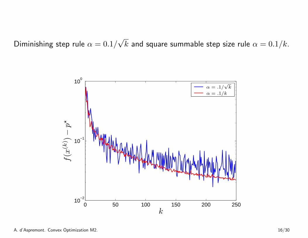
Diminishing step rule α = 0.1/√k and square summable step size rule α = 0.1/k.

0 50 100 150 200 25010

−2

10−1

100

α = .1/√k

α = .1/k

k

f(x

(k) )−

p⋆


Constant step length h = 0.02, diminishing step size rule α = 0.1/√k, and square

summable step rule α = 0.1/k

0 500 1000 1500 2000 2500 3000 350010

−3

10−2

10−1

100

h = 0.02

α = .1/√k

α = .1/k

k

f(k

)best−

p⋆


Gradient Descent


Gradient descent method

general descent method with ∆x = −∇f(x)

given a starting point x ∈ dom f .repeat

1. ∆x := −∇f(x).2. Line search. Choose step size t via exact or backtracking line search.3. Update. x := x+ t∆x.

until stopping criterion is satisfied.

� stopping criterion usually of the form ‖∇f(x)‖2 ≤ ε

� convergence result: for strongly convex f ,

f(x(k))− p? ≤ ck(f(x(0))− p?)

c ∈ (0, 1) depends on m, x(0), line search type.

� this means O(log 1/ε) iterations to get ε solution.

� very simple, but often very slow; rarely used in practice


quadratic problem in R2

f(x) = (1/2)(x21 + γx22) (γ > 0)

with exact line search, starting at x(0) = (γ, 1):

x(k)1 = γ

(γ − 1

γ + 1

)k

, x(k)2 =

(−γ − 1

γ + 1

)k

� very slow if γ � 1 or γ � 1

� example for γ = 10:

x1

x2

x(0)

x(1)

−10 0 10

−4

0

4


Accelerated Gradient Methods



Solveminimize f(x)subject to x ∈ C

in x ∈ Rn, with C ⊂ Rn convex.

� Additional smoothness assumption: the gradient is Lipschitz continuous

‖∇f(x)−∇f(y)‖ ≤ L‖x− y‖ for all x, y ∈ C

where ‖ · ‖ is the Euclidean norm (to simplify).



� Under this new smoothness assumption, we can improve the complexity boundfor the most basic gradient method

xk+1 = xk − h∇f(xk)

for some h > 0. We get

f(xk)− f(x∗) ≤ 2L(f(x0)− f(x∗))‖x0 − x∗‖2

2L‖x0 − x∗‖2 + k(f(x0)− f(x∗))

having set h = 1/L.

� Roughly O(1/ε) iterations to get ε-solution. This is suboptimal as the lowercomplexity bound is O(1/

√ε). In what follows, we will see how to reach this

optimal complexity.



The fact that the gradient ∇f(x) is Lipschitz continuous

‖∇f(x)−∇f(y)‖ ≤ L‖x− y‖ for all x, y ∈ C

has important algorithmic consequences:

� For any x, y ∈ Rn,

f(y) ≤ f(x) +∇f(x)T (y − x) +L

2‖y − x‖2

and we get a quadratic upper bound on the function f(x).

� This means in particular that if y = x− 1L∇f(x), then

f(y) ≤ f(x)− 1

2L‖∇f(x)‖2

and we get a guaranteed decrease in the function value at each gradient step.



We construct an estimate sequence φk(x) of the function f(x), together withsequences xk ∈ Rn and λk ≥ 0, satisfying

φk(x) ≤ (1− λk)f(x) + λkφ0(x)

andf(xk) ≤ φ∗k , min

x∈Rnφk(x).

This means in particular that

f(xk)− f∗ ≤ λk(φ0(x∗)− f∗)

(just plug x∗ in the inequalities above) so we get convergence if λk → 0.



The function f(x) and its estimate functions φk(x):

φ0(x)

φk(x)

φ∗k

(1− λk)f(x) + λkφ0(x)

f(x)

The functions are φk(x) are increasingly precise approximations of f(x) aroundthe optimum and are easier to minimize.



Intuition behind the method. Use the fact that the gradient is Lipschitzcontinuous.

� The inequality

f(y) ≤ f(x) +∇f(x)T (y − x) +L

2‖y − x‖2

helps us build the bounds φk(x).

� In fact, we can pickφk(x) = φ∗k + γk‖x− vk‖2

for some γk ≥ 0 and vk ∈ Rn.

� We get the points xk+1 by making a gradient step starting around theminimum of φk(x) (easy to compute), using the guarantee

f(y) ≤ f(x)− 1

2L‖∇f(x)‖2



Also solves minimization problems over simple convex sets C ⊂ Rn. Define thegradient mapping

gC(y, γ) = γ(y − xC(y, γ))

wherexC(y, γ) = argmin

x∈C

(f(y) +∇f(y)T (x− y) +

γ

2‖x− y‖2

)� Here, gC(y, γ) plays the role of the gradient for constrained problems, and

satisfies

f(x) ≥ f(xC(y, γ)) + gC(y, γ)T (x− y) +1

2γ‖gC(y, γ)‖2 +

µ

2‖x− y‖2

� This means in particular

f(xC(y, γ)) ≤ f(y)− 1

2γ‖gC(y, γ)‖2

(just set y = x in the previous inequality).



Minimize f(x) over C ⊂ Rn. Assuming ∇f(x) is Lipschitz continuous withconstant L and that f(x) is strongly convex with parameter µ ≥ 0.

� Choose x0 ∈ Rn and α0 ∈ (0, 1), set y0 = x0 and q = µ/L.

� For k = 1, . . . , kmax iterate

1. Compute ∇f(yk) and set

xk+1 = xC(yk, γ)

2. Compute αk+1 ∈ (0, 1) by solving

α2k+1 = (1− αk+1)α

2k + qαk+1

3. Update the current point, with

yk+1 = xk+1 +αk(1− αk)

α2k + αk+1

(xk+1 − xk)



Suppose we set α0 ≥√µ/L, we have the following complexity bound

f(xk)− f∗ ≤ ∆0 min

{(1−

√µ

L

)k

,4L

(2√L+ k

√γ0)2

}

where

∆0 =(f(x0)− f∗ +

γ02‖x0 − x∗‖2

)and γ0 =

α0(α0L− µ)

1− α0.

When the strong convexity parameter µ = 0, this means roughly O(1/√ε)

iterations to get an ε solution.

Remarks:

� The iterates yk are not guaranteed to be feasible (in some case, f(x) is notdefined outside of C).

� The norm ‖ · ‖ is Euclidean. Using other norms is sometimes more efficient.

Both issues can be remedied using an extra minimization subproblem.


Convex Optimization M2 - École Normale Supérieureaspremon/PDF/MVA/FirstOrderMethods.pdf · Convex...

Documents

Transcript of Convex Optimization M2 - École Normale Supérieureaspremon/PDF/MVA/FirstOrderMethods.pdf · Convex...