Convex formulations of inverse modeling problems on ...

Convex formulations of inverse modeling problems on

systems modeled by Hamilton-Jacobi equations:

applications to traffic flow engineering

Christian Claudel

Electrical Engineering and Computer SciencesUniversity of California at Berkeley

Technical Report No. UCB/EECS-2011-5

http://www.eecs.berkeley.edu/Pubs/TechRpts/2011/EECS-2011-5.html

January 20, 2011

Copyright © 2011, by the author(s).All rights reserved.

Permission to make digital or hard copies of all or part of this work forpersonal or classroom use is granted without fee provided that copies arenot made or distributed for profit or commercial advantage and that copiesbear this notice and the full citation on the first page. To copy otherwise, torepublish, to post on servers or to redistribute to lists, requires prior specificpermission.

Acknowledgement

I gratefully acknowledge Professors Bayen (CEE) and Tomlin (EECS) fortheir guidance.

Convex formulations of inverse modeling problems on systems modeled byHamilton-Jacobi equations: applications to traffic flow engineering

by

Christian G. Claudel

A dissertation submitted in partial satisfaction of the

requirements for the degree of

Doctor of Philosophy

in

Engineering - Electrical Engineering and Computer Sciences

in the

Graduate Division

of the

University of California, Berkeley

Committee in charge:

Professor Claire J. Tomlin, ChairAssociate Professor Alexandre M. Bayen

Professor Laurent El-Ghaoui

Fall 2010

Convex formulations of inverse modeling problems on systems modeled byHamilton-Jacobi equations: applications to traffic flow engineering

Copyright 2010by

Christian G. Claudel

1

Abstract

Convex formulations of inverse modeling problems on systems modeled by Hamilton-Jacobiequations. Applications to traffic flow engineering

by

Christian Claudel

Doctor of Philosophy in Engineering - Electrical Engineering and Computer Sciences

University of California, Berkeley

Professor Claire Jennifer Tomlin, Chair

This dissertation presents a new convex optimization-based estimation framework forsystems modeled by scalar Hamilton-Jacobi equations. Leveraging the control frameworkof viability theory, we characterize the solutions to the Hamilton-Jacobi equation by a Lax-Hopf formula, and show that the solution satisfies an inf-morphism property. These twoproperties, enable us to construct a semi-analytic formula for the solution associated withpiecewise affine initial, boundary and internal conditions. The semi-analytic solution isthe first major contribution of the thesis. This enables the construction of a scheme whichprovides numerical solutions of the partial differential equation. In addition to being gridless,the semi-analytic numerical scheme has two main advantages over standard computationalmethods: it is both exact and very fast.

Using the semi-analytic formulation of the solution, we also prove that the Hamilton-Jacobi equation restricts the possible values that the piecewise affine initial, boundary andinternal conditions can take, and that the corresponding set of possible values can be ex-pressed in the form of convex constraints. This enables the creation of a framework forsolving inverse modeling problems on systems modeled by Hamilton-Jacobi equations usinglinear programming, which is a contribution of the thesis. The formulation of these inversemodeling problems as convex programs was previously unknown. More generally, the thesisoutlines a series of problems, which can now be cast in convex form, thanks to the semi-analytic solution proposed in the first part of the thesis. We apply this framework to solvingseveral inverse modeling and estimation problems arising in transportation engineering, us-ing experimental data from fixed sensors and mobile GPS devices. The problems that canbe solved using linear programming include four classes of problems: data consistency veri-fication, data assimilation, data reconciliation, and coefficient estimation. Data consistencyverification is used to check if the measurements are compatible with the model assump-tions, and are applied to sensor fault detection for instance. Data assimilation and datareconciliation techniques enable the estimation of the state of the system in situations for

2

which the model constraints are incompatible with the measurement constraints. When themodel and data constraints are compatible, some quantities related to the state (for instancetravel time in the context of transportation engineering) can be estimated using coefficientestimation.

i

To Coralie...

ii

Contents

List of Figures v

1 Introduction 11.1 Background . . . . . . . . . . . . . . . . . . . . . . . . . . . . . . . . . . . . 11.2 Partial differential equation models of large scale infrastructure systems . . . 21.3 Control and estimation of partial differential equations . . . . . . . . . . . . 2

1.3.1 Filtering based methods . . . . . . . . . . . . . . . . . . . . . . . . . 21.3.2 Other methods . . . . . . . . . . . . . . . . . . . . . . . . . . . . . . 3

1.4 Hamilton-Jacobi equations . . . . . . . . . . . . . . . . . . . . . . . . . . . . 41.5 Numerical analysis for Hamilton-Jacobi equations . . . . . . . . . . . . . . . 41.6 Contributions . . . . . . . . . . . . . . . . . . . . . . . . . . . . . . . . . . . 51.7 Structure of the dissertation . . . . . . . . . . . . . . . . . . . . . . . . . . . 6

2 Fast and exact semi-analytic schemes for scalar Hamilton-Jacobi partialdifferential equations 82.1 Macroscopic highway traffic modeling . . . . . . . . . . . . . . . . . . . . . . 8

2.1.1 State of the art . . . . . . . . . . . . . . . . . . . . . . . . . . . . . . 82.1.2 First order scalar conservation laws . . . . . . . . . . . . . . . . . . . 92.1.3 Hamilton Jacobi equations with concave Hamiltonians . . . . . . . . 92.1.4 Hamiltonian . . . . . . . . . . . . . . . . . . . . . . . . . . . . . . . . 10

2.2 Value conditions . . . . . . . . . . . . . . . . . . . . . . . . . . . . . . . . . . 122.2.1 General definition . . . . . . . . . . . . . . . . . . . . . . . . . . . . . 122.2.2 Initial, boundary and internal conditions . . . . . . . . . . . . . . . . 13

2.3 Viability formulation of the solution . . . . . . . . . . . . . . . . . . . . . . . 142.3.1 Barron-Jensen/Frankowska solutions . . . . . . . . . . . . . . . . . . 142.3.2 Viability characterization of Barron-Jensen/Frankowska solutions . . 142.3.3 The Lax-Hopf formula . . . . . . . . . . . . . . . . . . . . . . . . . . 20

2.4 Properties of the Barron-Jensen/Frankowska solutions to Hamilton-Jacobiequations . . . . . . . . . . . . . . . . . . . . . . . . . . . . . . . . . . . . . 222.4.1 Domain of definition . . . . . . . . . . . . . . . . . . . . . . . . . . . 222.4.2 The inf-morphism property . . . . . . . . . . . . . . . . . . . . . . . 24

iii

2.4.3 Convexity property of the solutions associated with convex value con-ditions . . . . . . . . . . . . . . . . . . . . . . . . . . . . . . . . . . . 25

2.5 Analytic solutions associated with affine initial, boundary and internal condi-tions . . . . . . . . . . . . . . . . . . . . . . . . . . . . . . . . . . . . . . . . 272.5.1 Analytic Lax-Hopf formula associated with an affine initial condition 272.5.2 Analytic Lax-Hopf formula associated with an affine upstream bound-

ary condition . . . . . . . . . . . . . . . . . . . . . . . . . . . . . . . 302.5.3 Analytic Lax-Hopf formula associated with an affine downstream bound-

ary condition . . . . . . . . . . . . . . . . . . . . . . . . . . . . . . . 342.5.4 Analytic Lax-Hopf formula associated with an affine internal condition 38

2.6 Extension to piecewise affine initial, boundary and internal conditions . . . . 442.6.1 Semi-analytic solutions . . . . . . . . . . . . . . . . . . . . . . . . . . 442.6.2 Lax Hopf algorithm . . . . . . . . . . . . . . . . . . . . . . . . . . . . 45

2.7 Extension to scalar conservation laws . . . . . . . . . . . . . . . . . . . . . . 462.7.1 Spatial derivatives of the solutions to affine initial, boundary and in-

ternal conditions . . . . . . . . . . . . . . . . . . . . . . . . . . . . . 462.7.2 Computation of the density function . . . . . . . . . . . . . . . . . . 472.7.3 Extension of the Lax-Hopf algorithm for scalar conservation laws . . 48

2.8 Numerical examples . . . . . . . . . . . . . . . . . . . . . . . . . . . . . . . . 502.8.1 Integration of internal conditions into Hamilton-Jacobi equations . . 502.8.2 Numerical validation of the Lax-Hopf algorithm (density function) . . 512.8.3 Comparison with standard numerical schemes . . . . . . . . . . . . . 53

3 Convex formulations of the model constraints in Hamilton-Jacobi partialdifferential equations 553.1 Model constraints for well-posedness . . . . . . . . . . . . . . . . . . . . . . 55

3.1.1 Compatibility conditions . . . . . . . . . . . . . . . . . . . . . . . . . 583.1.2 Sufficient conditions on the Hamiltonian for compatibility of true value

conditions . . . . . . . . . . . . . . . . . . . . . . . . . . . . . . . . . 593.2 Properties of the model compatibility constraints . . . . . . . . . . . . . . . 63

3.2.1 Concavity property of the solutions with respect to their coefficients . 633.2.2 Convex formulation of the model compatibility constraints . . . . . . 653.2.3 Monotonicity property of the model compatibility conditions . . . . . 66

4 Applications 674.1 Traffic flow measurement data and value conditions . . . . . . . . . . . . . . 67

4.1.1 Fixed detector data . . . . . . . . . . . . . . . . . . . . . . . . . . . . 674.1.2 Mobile sensor data . . . . . . . . . . . . . . . . . . . . . . . . . . . . 684.1.3 Experimental setup . . . . . . . . . . . . . . . . . . . . . . . . . . . . 684.1.4 Link between measurement data and value conditions . . . . . . . . . 69

iv

4.2 Explicit instantiation of the model compatibility conditions for triangularHamiltonians . . . . . . . . . . . . . . . . . . . . . . . . . . . . . . . . . . . 72

4.3 Data constraints . . . . . . . . . . . . . . . . . . . . . . . . . . . . . . . . . 764.4 Compatibility and consistency problems . . . . . . . . . . . . . . . . . . . . 76

4.4.1 Data and model compatibility problem . . . . . . . . . . . . . . . . . 774.4.2 Data consistency problem . . . . . . . . . . . . . . . . . . . . . . . . 77

4.5 Estimation problems . . . . . . . . . . . . . . . . . . . . . . . . . . . . . . . 784.5.1 Definition for general functions of traffic-related coefficients . . . . . . 784.5.2 Lower and upper bounds on traffic coefficients . . . . . . . . . . . . . 784.5.3 Guaranteed ranges for traffic coefficients estimation . . . . . . . . . . 83

4.6 Data assimilation and data reconciliation problems . . . . . . . . . . . . . . 844.6.1 Problem definition . . . . . . . . . . . . . . . . . . . . . . . . . . . . 844.6.2 Numerical example . . . . . . . . . . . . . . . . . . . . . . . . . . . . 85

4.7 Cybersecurity, sensor fault detection and privacy analysis problems . . . . . 874.7.1 Consistency problems applied to sensor failure detection . . . . . . . 874.7.2 Consistency problems applied to cybersecurity . . . . . . . . . . . . . 894.7.3 Privacy analysis problems . . . . . . . . . . . . . . . . . . . . . . . . 90

5 Conclusion 955.1 Contributions . . . . . . . . . . . . . . . . . . . . . . . . . . . . . . . . . . . 955.2 Open problems . . . . . . . . . . . . . . . . . . . . . . . . . . . . . . . . . . 96

5.2.1 Mathematical problems . . . . . . . . . . . . . . . . . . . . . . . . . . 965.2.2 Application problems . . . . . . . . . . . . . . . . . . . . . . . . . . . 96

5.3 Future work . . . . . . . . . . . . . . . . . . . . . . . . . . . . . . . . . . . . 97

Bibliography 98

v

List of Figures

1.1 Illustration of the state estimation procedure. . . . . . . . . . . . . . 6

2.1 Illustration of the flow-density relationship. . . . . . . . . . . . . . . . 112.2 Illustration of the Greenshields and trapezoidal Hamiltonians. . . . 122.3 Illustration of the convex transforms associated with the Green-

shields and trapezoidal Hamiltonians. . . . . . . . . . . . . . . . . . . . 162.4 Illustration of the auxiliary dynamical system used to construct the

solutions to the HJ PDE. . . . . . . . . . . . . . . . . . . . . . . . . . . 172.5 Illustration of a capture basin associated with an epigraphical target. 182.6 Illustration of a viability episolution. . . . . . . . . . . . . . . . . . . . 192.7 Illustration of the domain of influence of a value condition. . . . . . 232.8 Illustration of the inf-morphism property. . . . . . . . . . . . . . . . . 242.9 Construction of the solution associated with an affine initial condition. 302.10 Construction of the solution associated with an affine upstream

boundary condition. . . . . . . . . . . . . . . . . . . . . . . . . . . . . . . 342.11 Construction of the solution associated with an affine downstream

boundary condition. . . . . . . . . . . . . . . . . . . . . . . . . . . . . . . 382.12 Construction of the solution associated with an affine internal con-

dition. . . . . . . . . . . . . . . . . . . . . . . . . . . . . . . . . . . . . . . . 442.13 Example of integration of an internal condition into the solution of

the HJ PDE (2.5). . . . . . . . . . . . . . . . . . . . . . . . . . . . . . . . 512.14 Comparison between the Lax-Hopf algorithm and the analytical so-

lution of problem (2.97). . . . . . . . . . . . . . . . . . . . . . . . . . . . 522.15 Computational time comparison between the Lax-Hopf algorithm

and the Godunov scheme (2.97). . . . . . . . . . . . . . . . . . . . . . . 53

3.1 NGSIM experimental data. . . . . . . . . . . . . . . . . . . . . . . . . . 563.2 Illustration of an upper estimate function ψ0(·). . . . . . . . . . . . . . 62

4.1 Experiment site layout. . . . . . . . . . . . . . . . . . . . . . . . . . . . . 69

vi

4.2 Illustration of the domains of the possible value conditions used toconstruct the solution of the Moskowitz HJ PDE. . . . . . . . . . . . 70

4.3 Initial number of vehicles estimation using linear programming. . . 794.4 Travel time estimation using linear programming. . . . . . . . . . . . 824.5 Solutions to data assimilation and data reconciliation problems. . . 864.6 Faulty sensor detection. . . . . . . . . . . . . . . . . . . . . . . . . . . . 884.7 Cyberattack detection using linear programming. . . . . . . . . . . . 924.8 Illustration of the choice of a subset of measurement data. . . . . . 934.9 Vehicle reidentification using linear programming. . . . . . . . . . . . 94

vii

Acknowledgments

I would like first to express my deepest gratitude to my two advisors Professor AlexandreBayen and Professor Claire Tomlin for their help and support ever since I arrived to Berkeleyin 2007. I am forever indebted to Alexandre, who gave me the opportunity to join hisresearch group. During these years of PhD studies, Alexandre has been an exceptionalmentor, available to help me 24/7 in my research and sending me to the nicest conferencesaround. Alexandre also taught me more about myself than anybody else.

It has been an honor to be advised by Claire. Her vision and scientific achievements arean inspiration for all of us. Her outstanding teaching qualities motivated me to become aprofessor myself.

I would like to thank Professor Laurent El-Ghaoui for serving on my Dissertation Com-mittee and Professors Murat Arcak and Jean Walrand for serving on my Qualifying ExamCommittee.

Professors Jean-Pierre Aubin and Patrick Saint-Pierre are gratefully acknowledged fortheir vision and for their scientific generosity. Jean-Pierre suggested to me new ways of ap-proaching an old problem. His expertise in Hamilton-Jacobi equations was extremely helpfulfor deriving my results. Patrick’s advice on numerical computations was also invaluable.

I would also like to thank Professor Carlos Daganzo, who was the first to formulate thetraffic flow model used in this thesis as a Hamilton-Jacobi equation.

The Mobile Millennium gang was a fantastic team to work with. I would like to thankthe French connection (Aude, Julie, Pierre-Emmanuel, Sebastien, Timothy), the Chicagosyndicate (Dan, Matthieu, Olli-Pekka) and numerous other gangsters: Andrew, Mohammad,Ryan, Samitha, Saurabh and Tarek, for being so nice to work with. I will miss you all!

The support staff of the CCIT was also wonderful. Saneesh Apte, Joe Butler, DanielEdwards and Tom West have been working hard during the last three years to make MobileMillennium a success.

On a more personal note, I would like to thank my parents Jacques and Anne-Marie, andmy sisters Aurelia and Anne-Claire who always offered me their love, support and help.

Finally, my wife Coralie offered me her endless love during all these years at UC Berkeley,and the strength to overcome difficulties. I want to dedicate my thesis to her.

1

Chapter 1

Introduction

‘

1.1 Background

Traffic congestion is a major issue in urban environments. Regardless of its cause, it cre-ates both delays and increased fuel consumption, which has a major impact on the economy.In the United States alone, the cost traffic congestion is approximately $500 per driver peryear and the total annual cost of traffic congestion represents 0.5% of the GDP [43]. Sincecongestion occurs when user demand exceeds the infrastructure capacity, congestion can besolved by either increasing the infrastructure capacity (for instance building new roads),or reducing user demand (for instance through better traffic information systems). Withthe decreasing cost of sensors and the increasing number of computational platforms (forinstance GPS-enabled smartphones) that can act as sensors [101] themselves, there is nowan unprecedented amount of traffic data, which can be leveraged to provide better trafficinformation. This information in turn could be used to help reduce congestion, by providingtraffic management authorities with the proper tools to spread used demand over the daymore efficiently.

While increasing quantities of traffic measurement data become available, the problemof estimating traffic from significantly different data sources is very complex. The highwaynetwork is usually modeled as a distributed parameter system, which means that it can beviewed as an infinite dimensional system. In addition, the physics of traffic are known tobe nonlinear. Finally, measurement data comes from different types of sensors which do notnecessarily measure the same physical quantities. The main goal of this dissertation is toaddress the problem of integrating the constraints of the traffic model in a tractable manner,using a convex-optimization based framework. This framework is applied to solve variousestimation problems arising in transportation engineering, using experimental data.

2

1.2 Partial differential equation models of large scale

infrastructure systems

Large scale infrastructure systems, such as transportation networks, networked waterchannels, or air transportation networks are distributed parameter systems, that is, their stateis usually described by a function of space and time, in contrast to a finite dimensional vector.Another way to think about this would be as an “infinite dimensional” vector. A commonmathematical tool for modeling such systems is partial differential equations (PDEs). Theyprovide an efficient way of representing physical phenomena in a mathematically compactmanner, which integrates the distributed features of the systems of interest [44].

Among PDEs, a specific class stands out, conservation laws [71, 19], which model phe-nomena in which a balance equation governs the physics (for example mass balance, mo-mentum balance, charge balance, etc.). Water channels for instance can be modeled usingthe Saint-Venant PDE [73], obtained from the conservation of water mass and momentum.Examples of applications of such models can be found in [34, 84, 74, 34]. Ground [72, 86]and air transportation networks [92] can both be modeled by the Lighthill-Whitham-Richards(LWR) PDE, which is based on the conservation of vehicles. Alternatively, traffic flow canalso be modeled using second order models [33, 11, 81, 17, 100], which are non-scalar con-servation laws. All these PDEs and others used to describe distributed parameter systemsare not necessarily conservation laws however. In structural engineering for instance, beamdeformation can be modeled by the Euler-Bernoulli beam PDE [66], which is not a conser-vation law. In electrical engineering, the Telegraph equation [50] can be used to model wavepropagation in telecommunication lines, and is also not a conservation law.

1.3 Control and estimation of partial differential equa-

tions

1.3.1 Filtering based methods

State estimation and control for PDE-based systems is more complex than for theirordinary differential equation (ODE) based counterparts, because of the distributed natureof the state.

The tools available for estimating [90] and controlling [66] the states of an ODE can beextended to systems modeled by a PDE, for instance using variations of Kalman Filtering(KF), originally derived for systems modeled by linear ODEs [15]. Extended Kalman Filtering(EKF) [3] is a modification of Kalman filtering for nonlinear systems. EKF techniques havebeen applied to water channels state estimation problems in [46], and in traffic flow estimationproblems in [96, 3] for instance.

The EKF can however perform poorly for specific nonlinear systems, for which Monte

3

Carlo techniques are a possible alternative. For example, when the dynamics exhibits nons-moothness or nondifferentiability, EKF is known to have problems [97]. Monte Carlo methodsinvolve estimating the current probable value of the state, computing the state evolution, andcomparing it against new measurement data to obtain a current estimate. By their nature,Monte-Carlo based methods can apply to any model, albeit with some computational costpenalty. Ensemble Kalman Filtering (EnKF) [47] is a Monte-Carlo based method that canbe used for systems modeled by nonlinear PDEs, for instance the LWR [97] PDE, withoutapproximating the model around the current estimate as done in EKF. Other examples ofapplication of EnKF include Shallow Water Equations [94], or meteorology [62]. The EnKFsamples the possible current states of the system according to a probability distribution,computes the evolution of these samples, and combine these evolutions with new measure-ments to obtain the best estimate of the state. The Mobile Millennium system [101] isan example of operational implementation of the EnKF for traffic flow modeling using theLWR PDE. More generally, the state of distributed parameter systems can be estimatedusing Particle Filtering (PF), which can be used for general nonlinear systems, albeit witha higher computational cost [26].

1.3.2 Other methods

Backstepping methods [66] are control design methods that can be applied to some classesof nonlinear systems. They involve designing a controller for a known-stable system and“back out” new controllers that progressively stabilize each outer supersystem.

The theory of differential flatness, which was originally developed in [49], consists ina parametrization of the trajectories of a system by one of its outputs, called the “flatoutput” [82, 1]. It can be used to control the state of water channels [85] for instance.

Lyapunov methods [65] are based the extension of the Lyapunov theory for ODE-basedsystems to the PDE case. Similarly to ODE-based systems, they involve the use of a Lya-punov function associated with the state of the system, and which is either bounded ordecreasing.

Machine learning methods [63] in contrast rely on experimental datasets to learn howthe state evolves. One of the main focuses of machine learning methods is to automaticallylearn to recognize specific patterns using statistical methods [2]. Machine learning methodscan be applied to very different problems, including estimation problems [59] on systemsmodeled by PDEs.

Finally, spectral methods [99, 27] use modal decomposition techniques to transform dy-namic constraints into static constraints in the frequency domain, and subsequently obtaina static inverse modeling problem, which is easier to solve.

One of the major difficulties arising when dealing with sensing problems on systemsmodeled by PDEs is the integration of the model constraints into the estimation problem.The PDEs investigated in this dissertation are nonlinear. Their solutions can be nonsmoothand even discontinuous, which makes the model constraints difficult to derive. One of the

4

contributions of this dissertation is to express the model constraints as convex inequalities,which are both explicit and computationally tractable.

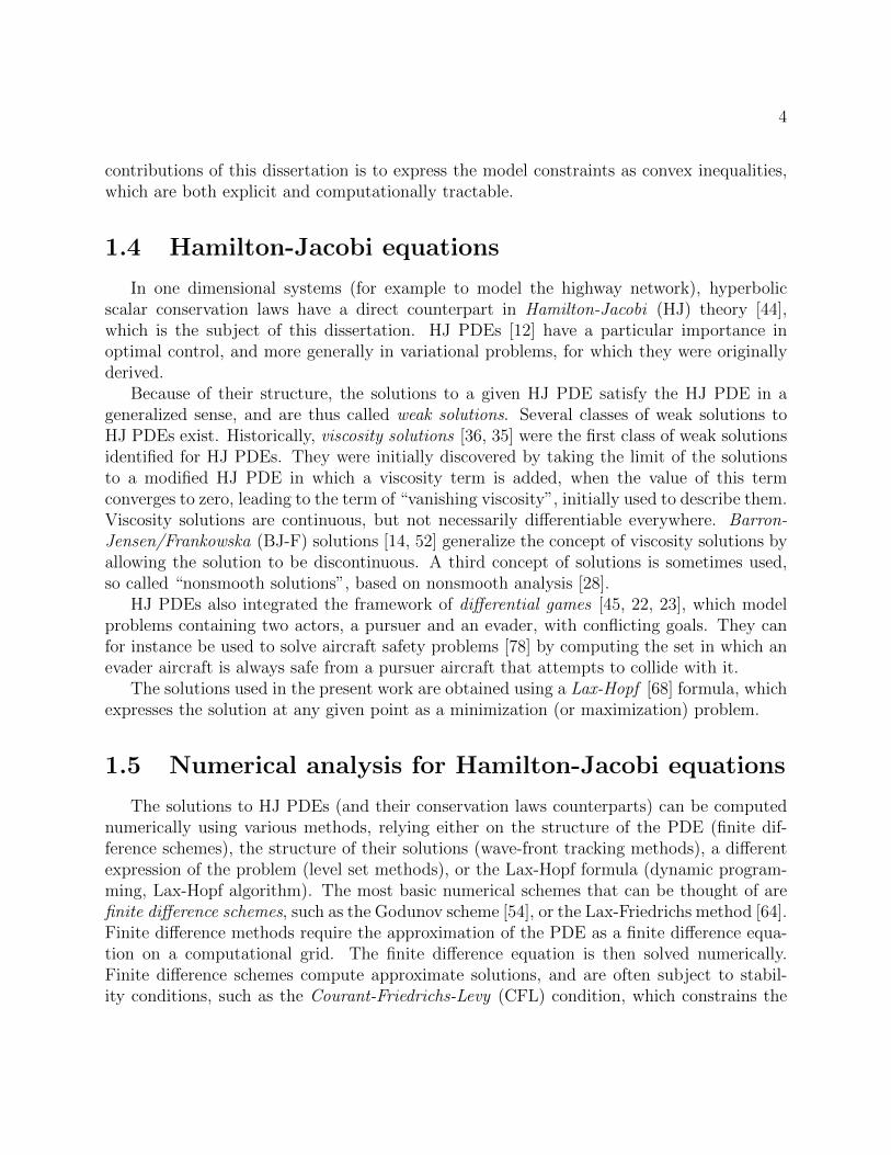
1.4 Hamilton-Jacobi equations

In one dimensional systems (for example to model the highway network), hyperbolicscalar conservation laws have a direct counterpart in Hamilton-Jacobi (HJ) theory [44],which is the subject of this dissertation. HJ PDEs [12] have a particular importance inoptimal control, and more generally in variational problems, for which they were originallyderived.

Because of their structure, the solutions to a given HJ PDE satisfy the HJ PDE in ageneralized sense, and are thus called weak solutions. Several classes of weak solutions toHJ PDEs exist. Historically, viscosity solutions [36, 35] were the first class of weak solutionsidentified for HJ PDEs. They were initially discovered by taking the limit of the solutionsto a modified HJ PDE in which a viscosity term is added, when the value of this termconverges to zero, leading to the term of “vanishing viscosity”, initially used to describe them.Viscosity solutions are continuous, but not necessarily differentiable everywhere. Barron-Jensen/Frankowska (BJ-F) solutions [14, 52] generalize the concept of viscosity solutions byallowing the solution to be discontinuous. A third concept of solutions is sometimes used,so called “nonsmooth solutions”, based on nonsmooth analysis [28].

HJ PDEs also integrated the framework of differential games [45, 22, 23], which modelproblems containing two actors, a pursuer and an evader, with conflicting goals. They canfor instance be used to solve aircraft safety problems [78] by computing the set in which anevader aircraft is always safe from a pursuer aircraft that attempts to collide with it.

The solutions used in the present work are obtained using a Lax-Hopf [68] formula, whichexpresses the solution at any given point as a minimization (or maximization) problem.

1.5 Numerical analysis for Hamilton-Jacobi equations

The solutions to HJ PDEs (and their conservation laws counterparts) can be computednumerically using various methods, relying either on the structure of the PDE (finite dif-ference schemes), the structure of their solutions (wave-front tracking methods), a differentexpression of the problem (level set methods), or the Lax-Hopf formula (dynamic program-ming, Lax-Hopf algorithm). The most basic numerical schemes that can be thought of arefinite difference schemes, such as the Godunov scheme [54], or the Lax-Friedrichs method [64].Finite difference methods require the approximation of the PDE as a finite difference equa-tion on a computational grid. The finite difference equation is then solved numerically.Finite difference schemes compute approximate solutions, and are often subject to stabil-ity conditions, such as the Courant-Friedrichs-Levy (CFL) condition, which constrains the

5

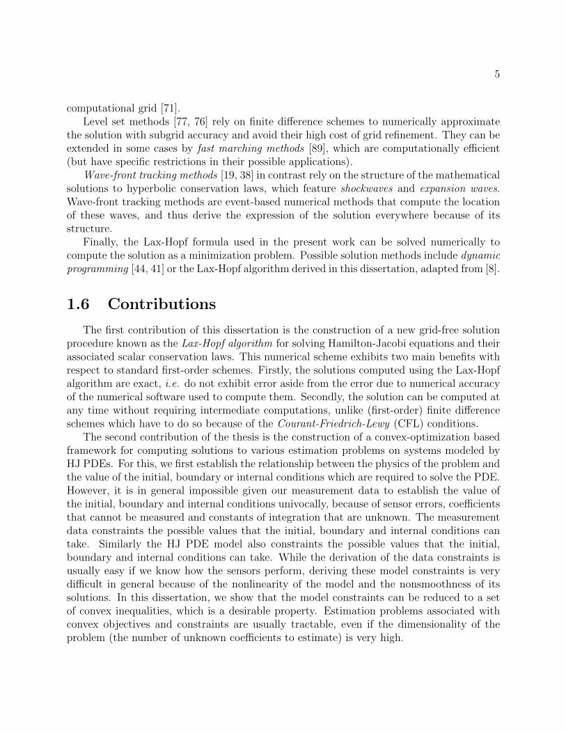
computational grid [71].Level set methods [77, 76] rely on finite difference schemes to numerically approximate

the solution with subgrid accuracy and avoid their high cost of grid refinement. They can beextended in some cases by fast marching methods [89], which are computationally efficient(but have specific restrictions in their possible applications).

Wave-front tracking methods [19, 38] in contrast rely on the structure of the mathematicalsolutions to hyperbolic conservation laws, which feature shockwaves and expansion waves.Wave-front tracking methods are event-based numerical methods that compute the locationof these waves, and thus derive the expression of the solution everywhere because of itsstructure.

Finally, the Lax-Hopf formula used in the present work can be solved numerically tocompute the solution as a minimization problem. Possible solution methods include dynamicprogramming [44, 41] or the Lax-Hopf algorithm derived in this dissertation, adapted from [8].

1.6 Contributions

The first contribution of this dissertation is the construction of a new grid-free solutionprocedure known as the Lax-Hopf algorithm for solving Hamilton-Jacobi equations and theirassociated scalar conservation laws. This numerical scheme exhibits two main benefits withrespect to standard first-order schemes. Firstly, the solutions computed using the Lax-Hopfalgorithm are exact, i.e. do not exhibit error aside from the error due to numerical accuracyof the numerical software used to compute them. Secondly, the solution can be computed atany time without requiring intermediate computations, unlike (first-order) finite differenceschemes which have to do so because of the Courant-Friedrich-Lewy (CFL) conditions.

The second contribution of the thesis is the construction of a convex-optimization basedframework for computing solutions to various estimation problems on systems modeled byHJ PDEs. For this, we first establish the relationship between the physics of the problem andthe value of the initial, boundary or internal conditions which are required to solve the PDE.However, it is in general impossible given our measurement data to establish the value ofthe initial, boundary and internal conditions univocally, because of sensor errors, coefficientsthat cannot be measured and constants of integration that are unknown. The measurementdata constraints the possible values that the initial, boundary and internal conditions cantake. Similarly the HJ PDE model also constraints the possible values that the initial,boundary and internal conditions can take. While the derivation of the data constraints isusually easy if we know how the sensors perform, deriving these model constraints is verydifficult in general because of the nonlinearity of the model and the nonsmoothness of itssolutions. In this dissertation, we show that the model constraints can be reduced to a setof convex inequalities, which is a desirable property. Estimation problems associated withconvex objectives and constraints are usually tractable, even if the dimensionality of theproblem (the number of unknown coefficients to estimate) is very high.

6

Figure 1.1: Illustration of the state estimation procedure.

The third contribution is the numerical implementation of this estimation frameworkillustrated in Figure 1.1 for solving various transportation engineering problems using exper-imental traffic data. The same framework can be used for very different problems, such asestimation problems (for instance travel time estimation), sensor fault detection problems, oruser privacy analysis. All these problems are posed as Linear Programs (LPs), a particularclass of convex-optimization problems for which numerous solvers exist [18].

1.7 Structure of the dissertation

The rest of this dissertation is organized as follows. We construct the Lax-Hopf algorithmintroduced as the backbone of our method, and present some of its benefits and applicationsin chapter 2. For this, section 2.1 introduces the HJ PDE model investigated in this disser-tation. Section 2.2 presents the notion of value condition, which encompasses the traditionalconcepts of initial and boundary as well as a new concept of internal conditions. We thenderive a possible method for solving the HJ PDE using the control framework of ViabilityTheory in section 2.3. This method enables us to define a Lax-Hopf formula, which charac-terizes the solution. In section 2.4, we describe the mathematical properties of the solution,derived from the structure of the Lax-Hopf formula. In particular, the inf-morphism prop-erty enables us to decompose a complex problem involving multiple initial, boundary andinternal conditions into more tractable subproblems. We then show in section 2.5 that thesubproblems, namely the problems of computing the solutions associated with affine initial,boundary and internal conditions can be solved exactly and explicitly. Using these solutions

7

and the inf-morphism property derived earlier, we build in section 2.6 a semi-analytic nu-merical scheme for solving the HJ PDE exactly and without requiring a computational grid.We also show in section 2.7 that a similar numerical scheme can be used to solve the corre-sponding scalar conservation laws. Numerical illustrations and a comparison with standardfirst-order numerical schemes are performed in section 2.8.

The derivation of the model constraints as convex inequalities on systems modeled byHJ PDEs is presented in Chapter 3. We derive the model constraints in section 3.1 andpresent some important properties of the model constraints in section 3.2. Using the Lax-Hopf formula, we show that the model constraints are convex, and can be written explicitly.The nature of the model constraints also imply an important monotonicity property withrespect to new data, which states that adding new data into the estimation problem canonly increase the accuracy of the solution.

The applications of this framework to practical problems are presented in Chapter 4. Wefirst establish the relationship between measurement data and initial, boundary and internalconditions in section 4.1. We then instantiate the model compatibility constraints explicitlyfor triangular Hamiltonians in section 4.2. We also derive the corresponding measurementdata constraints explicitly (in section 4.3). In section 4.4, we introduce two fundamentalconvex feasibility problems that can be used to determine if the model and data constraintsare compatible and if the measurement data is consistent with the physics of the problem.This is used in section 4.5 to present different estimation problems that can be solved usingLPs obtained by direct instantiation of the convex problems derived earlier. We show inparticular that some nonconvex estimation problems such as the travel time estimationproblem can still be decomposed as a series of LPs and thus are computationally tractable.In section 4.6, we define two important inverse modeling problems for situations in which thedata and model constraints are incompatible. These problems are respectively known as dataassimilation and data reconciliation, and are obtained by relaxing model and data constraintsrespectively. We then proceed to solve different problems of interest for transportationengineering. The examples presented in this dissertation involve experimental highway trafficdata sets, obtained from the Performance Measurement System (PeMS) and the MobileCentury experiment in California. Some of the resulting algorithms have been implementedin the Mobile Millennium system [101], in particular a sensor fault detection algorithmdetailed in section 4.7 that runs in real time, every 30s for all highways in northern California.

8

Chapter 2

Fast and exact semi-analytic schemesfor scalar Hamilton-Jacobi partialdifferential equations

2.1 Macroscopic highway traffic modeling

2.1.1 State of the art

Traffic flow models can be separated into at least two distinct classes, depending on thescale at which they describe traffic. Microscopic models such as the car following model [51],describe traffic at the individual vehicle level as a flow of particles. Their objective is toprovide a relationship between the velocity of a given vehicle and its environment. In con-trast, macroscopic models [56, 72, 86] describe traffic flow as a continuous medium and arerelated to fluid mechanics models. In this dissertation, we focus on the Lighthill-Whitham-Richards [72, 86] (LWR) model, which is a first order macroscopic flow model. Owing to itssimplicity and its robustness, the LWR model and its related cell transmission model [39, 40]are commonly used in transportation engineering [95, 41, 3, 97]. Note that macroscopicmodels are not necessarily first order models, see for instance [17]. Traffic flow can also bedescribed at an intermediate scale using mesoscopic models [21]. Mesoscopic models fol-low methods of statistical mechanics, and express the solution using an integro-differentialequation such as the Boltzmann equation [25].

Similarly to other large scale infrastructure systems such as the water channel network,the highway transportation network is a very complex graph containing highway sectionsconnected by junctions or splits. In this dissertation, we do not consider the effects of thenetwork and solely focus on the description of traffic flow on a highway section. Extendingthis framework to the whole transportation network [20, 53] requires the computation ofboundary conditions of each highway section, and is out of the scope of this thesis. Itis still a somewhat open problem which will require the generalization of weak boundary

9

conditions [13, 70], commonly used in traffic engineering [91, 97, 58].

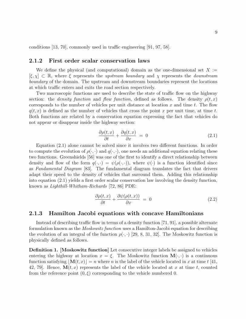
2.1.2 First order scalar conservation laws

We define the physical (and computational) domain as the one-dimensional set X :=[ξ, χ] ⊂ R, where ξ represents the upstream boundary and χ represents the downstreamboundary of the domain. The upstream and downstream boundaries represent the locationsat which traffic enters and exits the road section respectively.

Two macroscopic functions are used to describe the state of traffic flow on the highwaysection: the density function and flow function, defined as follows. The density ρ(t, x)corresponds to the number of vehicles per unit distance at location x and time t. The flowq(t, x) is defined as the number of vehicles that cross the point x per unit time, at time t.Both functions are related by a conservation equation expressing the fact that vehicles donot appear or disappear inside the highway section:

∂ρ(t, x)

∂t+∂q(t, x)

∂x= 0 (2.1)

Equation (2.1) alone cannot be solved since it involves two different functions. In orderto compute the evolution of ρ(·, ·) and q(·, ·), one needs an additional equation relating thesetwo functions. Greenshields [56] was one of the first to identify a direct relationship betweendensity and flow of the form q(·, ·) = ψ(ρ(·, ·)), where ψ(·) is a function identified sinceas Fundamental Diagram [83]. The fundamental diagram translates the fact that driversadapt their speed to the density of vehicles that surround them. Adding this relationshipinto equation (2.1) yields a first order scalar conservation law involving the density function,known as Lighthill-Whitham-Richards [72, 86] PDE:

∂ρ(t, x)

∂t+∂ψ(ρ(t, x))

∂x= 0 (2.2)

2.1.3 Hamilton Jacobi equations with concave Hamiltonians

Instead of describing traffic flow in terms of a density function [71, 91], a possible alternateformulation known as the Moskowitz function uses a Hamilton-Jacobi equation for describingthe evolution of an integral of the function ρ(·, ·) [29, 8, 31, 32]. The Moskowitz function isphysically defined as follows.

Definition 1. [Moskowitz function] Let consecutive integer labels be assigned to vehiclesentering the highway at location x = ξ. The Moskowitz function M(·, ·) is a continuousfunction satisfying bM(t, x)c = n where n is the label of the vehicle located in x at time t [41,42, 79]. Hence, M(t, x) represents the label of the vehicle located at x at time t, countedfrom the reference point (0, ξ) corresponding to the vehicle numbered 0.

10

The properties of the Moskowitz function have been extensively studied, for instance inthe famous Newell trilogy [80]. The formal link between the density function ρ(·, ·), the flowfunction q(·, ·) and the Moskowitz function M(·, ·) is given by:

M(t2, x2)−M(t1, x1) =

∫ x2

x1

−ρ(t1, x)dx+

∫ t2

t1

q(t, x2)dt (2.3)

Conversely, the flow and density functions q(·, ·) and ρ(·, ·) are related to the spatial andtemporal derivatives of the Moskowitz function M(·, ·):

q(t, x) = ∂M(t,x)∂t

ρ(t, x) = −∂M(t,x)∂x

(2.4)

The Moskowitz function M(·, ·) solves the following equation, obtained by combining (2.4)and the LWR PDE (2.2):

∂M(t, x)

∂t− ψ

(−∂M(t, x)

∂x

)= 0 (2.5)

Equation (2.5) is an Hamilton-Jacobi (HJ) PDE [35, 8]. In the context of HJ PDEs, theparameter ψ(·) is known as Hamiltonian, while it is known as fundamental diagram in thecontext of the LWR PDE (2.2) and traffic engineering [39].

2.1.4 Hamiltonian

The LWR PDE (2.2) and its associated HJ PDE (2.5) are both characterized by a Hamil-tonian ψ(·), which describes the relationship between density and flow. For low densities,

the average velocity of traffic v(·, ·) = q(·,·)ρ(·,·) is close to maximal velocity allowed on the road

section, denoted by ν[. As the density increases, traffic velocity progressively drops andvanishes for the maximal density ω that the highway section can contain and known as jamdensity. Hence, the Hamiltonian ψ(·) satisfies the following properties:

• limρ→0

ψ(ρ)

ρ= ν[

• the function ρ→ ψ(ρ)ρ

is decreasing

• ψ(ω) = 0

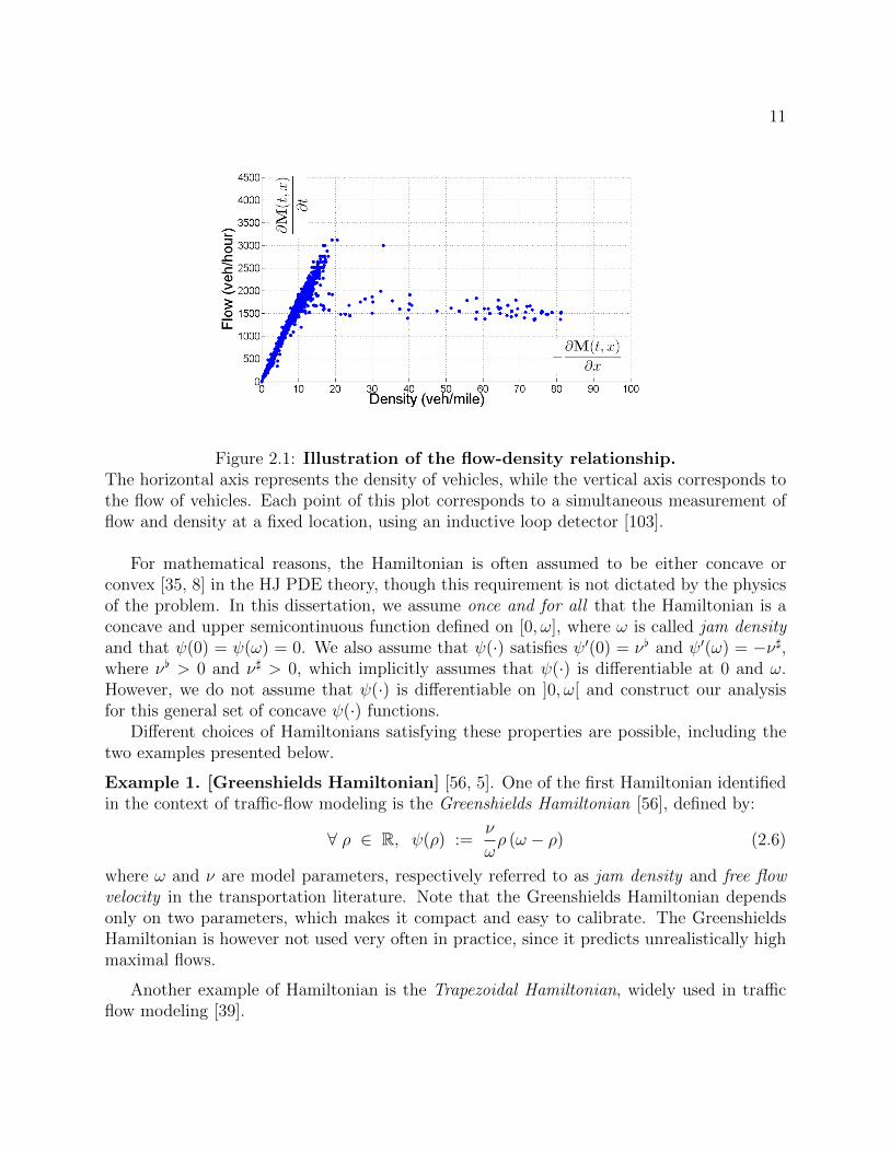
An example of flow-density plot using experimental data from the Performance Measure-ment System (PeMS) [103] is shown in Figure 2.1.

11

Figure 2.1: Illustration of the flow-density relationship.The horizontal axis represents the density of vehicles, while the vertical axis corresponds tothe flow of vehicles. Each point of this plot corresponds to a simultaneous measurement offlow and density at a fixed location, using an inductive loop detector [103].

For mathematical reasons, the Hamiltonian is often assumed to be either concave orconvex [35, 8] in the HJ PDE theory, though this requirement is not dictated by the physicsof the problem. In this dissertation, we assume once and for all that the Hamiltonian is aconcave and upper semicontinuous function defined on [0, ω], where ω is called jam densityand that ψ(0) = ψ(ω) = 0. We also assume that ψ(·) satisfies ψ′(0) = ν[ and ψ′(ω) = −ν],where ν[ > 0 and ν] > 0, which implicitly assumes that ψ(·) is differentiable at 0 and ω.However, we do not assume that ψ(·) is differentiable on ]0, ω[ and construct our analysisfor this general set of concave ψ(·) functions.

Different choices of Hamiltonians satisfying these properties are possible, including thetwo examples presented below.

Example 1. [Greenshields Hamiltonian] [56, 5]. One of the first Hamiltonian identifiedin the context of traffic-flow modeling is the Greenshields Hamiltonian [56], defined by:

∀ ρ ∈ R, ψ(ρ) :=ν

ωρ (ω − ρ) (2.6)

where ω and ν are model parameters, respectively referred to as jam density and free flowvelocity in the transportation literature. Note that the Greenshields Hamiltonian dependsonly on two parameters, which makes it compact and easy to calibrate. The GreenshieldsHamiltonian is however not used very often in practice, since it predicts unrealistically highmaximal flows.

Another example of Hamiltonian is the Trapezoidal Hamiltonian, widely used in trafficflow modeling [39].

12

Example 2. [Trapezoidal Hamiltonian] [39, 40, 93]. The trapezoidal Hamiltonian iscommonly used to model the hybrid nature of traffic flow propagation:

ψ(ρ) =

ν[ρ if ρ ≤ γ[

δ if ρ ∈ [γ[, γ]]ν](ω − ρ) if ρ ≥ γ]

where ν[, ν], ω, δ, γ[ and γ] are constants and satisfy the following relations: δ ≤ ων[ν]

ν[+ν]

(called capacity in the transportation engineering literature),γ[ := δν[

(called lower critical

density in the transportation engineering literature) and γ] := ν]ω−δν]

(called upper critical

density in the transportation engineering literature). When γ[ = γ], the Hamiltonian istriangular, as used in the applications of Chapter 4.

The Greenshields and trapezoidal Hamiltonians are illustrated in Figure 2.2.

Figure 2.2: Illustration of the Greenshields and trapezoidal Hamiltonians.Numerical values are represented in the context of transportation, i.e. the variable ρ ishomogeneous to the vehicle density (in percent of the maximal density). The Hamiltonianψ(ρ) is represented in vehicles per hour. Left: representation of a Greenshields Hamiltonian.Right: representation of a trapezoidal Hamiltonian.

Solving the HJ PDE (2.5) requires the definition of value conditions, which we now define.

2.2 Value conditions

2.2.1 General definition

Value conditions encompass the traditional concepts of initial, boundary and internalconditions and are defined as follows.

13

Definition 2. [Value condition] A value condition c(·, ·) is a lower semicontinuous functiondefined on a subset of [0, tmax]×X.

By convention, a value condition c(·, ·) as defined in definition 2 satisfies c(t, x) = +∞if (t, x) /∈ Dom(c). The domain of definition of a value condition represents the subset ofthe space time domain R+ × X in which we want the value condition to apply. Differenttypes of value condition exist, including the traditional initial, upstream and downstreamboundary conditions [8, 39]. More complex value conditions do exist however. Internalconditions consist in value condition whose domains of definition are connected and of emptyinterior [41, 69]. Hybrid conditions [29] are the most general type of value condition, but areout of the scope of this dissertation.

2.2.2 Initial, boundary and internal conditions

Initial, boundary are common in problems involving PDEs. Internal conditions are spe-cific to the problem introduced in this thesis, though it applies to numerous other fields.These value conditions are defined as follows.

Definition 3. [Initial condition] An initial condition is a value condition c(·, ·) definedon Dom(c) := {0} ×X.

Note that the traditional Cauchy problem consists in finding the solution to (2.5) associ-ated with a value condition defined on {0}×R, i.e. an initial condition defined on an infinitespatial domain.

In contrast, the upstream and downstream boundary conditions are related to the valueof the state on the boundaries of the physical domain.

Definition 4. [Upstream and downstream boundary conditions] An upstream bound-ary condition is a value condition c(·, ·) defined on the set Dom(c) := [0, tmax]×{ξ}. A down-stream boundary condition is a value condition c(·, ·) defined on Dom(c) := [0, tmax]× {χ}.

Note that the traditional mixed Initial-Boundary conditions problem [91] consists in find-ing the solution to (2.5) associated with a value condition defined on {0} ×X ∪R+ × {ξ} ∪R+ × {χ}, i.e. an initial condition, an upstream boundary condition and a downstreamboundary condition defined on an infinite temporal domain.

Note that the initial, upstream and downstream boundary conditions are all defined at theboundary of the computational domain [0, tmax] × X. Since probe measurements originatefrom the interior of the computational domain, a specific type of value condition, knownas internal condition has to be defined as follows.

Definition 5. [Internal condition] An internal condition is a value condition c(·, ·) definedon a domain of the form Dom(c) := {(t, xv(t)), t ∈ Dom(xv)}, where xv(·) is a function of[0, tmax].

14

In definition 5, the function xv(·) represents the velocity function associated with theinternal condition. The set {(t, xv(t)), t ∈ Dom(xv)} is the trajectory associated with theinternal condition.

Note that in the applications of this dissertation, measurement data alone is not sufficientto define the value conditions unambiguously, since some of coefficients used to build thesevalue conditions are impossible to measure, or are not perfectly known due to measurementerrors.

We now present a characterization of the solutions to the HJ PDE (2.5) associated withthe value conditions defined earlier. This characterization uses Viability theory, an areaof optimal control studying the evolution of dynamical systems evolving under state con-straints [6, 7] known as viability constraints.

2.3 Viability formulation of the solution

2.3.1 Barron-Jensen/Frankowska solutions

As mentioned earlier, several classes of solutions to HJ PDEs exist. Viscosity solu-tions [35] to HJ PDEs are continuous functions. The specific type of solutions to (2.5) thatwe consider in the present work is the Barron-Jensen/Frankowska (B-J/F) solutions [14, 52].B-J/F solutions extend the concept of viscosity solutions by allowing the solution to be lowersemicontinuous. Note that both concepts are identical for mixed initial-boundary conditionsproblems involving Lipschitz-continuous initial and boundary conditions [52].

The B-J/F solutions to (2.5) can be derived using the control framework of Viabilitytheory [6], presented in the following section.

2.3.2 Viability characterization of Barron-Jensen/Frankowska so-lutions

We now introduce some tools used in the context of viability theory [6, 7], which areessential building blocks for the work presented here.

Definition 6. [6, 7] [Capture basin] Given a dynamical system F and two sets K(called the constraint set) and C (called the target set) satisfying C ⊂ K, the capture basinCaptF (K, C) is the subset of states of K from which there exists at least one evolution solutionto F reaching the target C in finite time while remaining in K.

Note that the capture basin associated with a given dynamical system, constraint andtarget set can be numerically computed using the Capture Basin Algorithm [22, 23, 88]. Inorder to properly define the dynamical system used to construct B-J/F solutions to (2.5),we first need to define a convex transform ϕ∗(·) of the Hamiltonian ψ(·) as follows.

15

Definition 7. [Convex transform] Given a concave and upper semicontinuous functionψ(·) with domain Dom(ψ), we define the convex transform ϕ∗(·) of ψ(·) as follows:

ϕ∗(u) := supp∈Dom(ψ)

[p · u+ ψ(p)] (2.7)

The inverse transform of a convex and lower semicontinuous function ϕ∗(·) is defined [8]by:

ψ(p) := infu∈Dom(ϕ∗)

[ϕ∗(u)− p · u] (2.8)

Note that equation (2.7) in definition 7 differs from the traditional definition of theLegendre-Fenchel transform by a sign change.

The function ϕ∗(·) defined by (2.7) is convex as the pointwise supremum of affine func-tions [18, 87] and is defined on the interval Dom(ϕ∗) := [−ν[, ν]]. Since ϕ∗(·) is convex,it is subdifferentiable [18] on [−ν[, ν]] and its subderivative satisfies the Legendre-Fenchelinversion formula [8]:

u ∈ −∂+ψ(ρ) if and only if ρ ∈ ∂−ϕ∗(u) (2.9)

in which, following [18], we use the following definition of the subderivative ∂−(·) and thesuperderivative ∂+(·):

v ∈ ∂−F(x0) if and only if ∀x ∈ Dom (F) , F(x) ≥ F(x0) + v(x− x0) (2.10)

v ∈ ∂+F(x0) if and only if ∀x ∈ Dom (F) , F(x) ≤ F(x0) + v(x− x0) (2.11)

Note that any convex (respectively concave) function F(·) is subdifferentiable (respec-tively superdifferentiable) on its domain of definition [18].

The convex transform satisfies ϕ∗(−ν[) := supp∈Dom(ψ)

[−pν[ + ψ(p)] = 0 since ψ(·) is

concave and satisfies ψ′(0) = ν[. In addition, it is positive by (2.7) since ψ(0) = 0 and0 ∈ [0, ω].

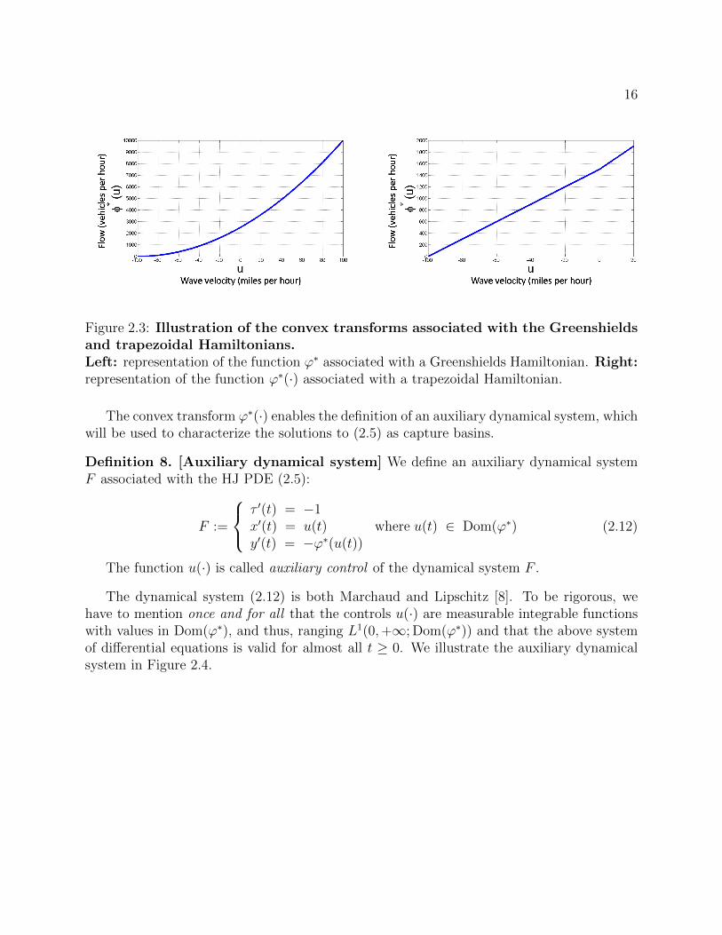
The convex transforms associated with Greenshields and trapezoidal Hamiltonians de-fined in section 2.1.4 are represented in Figure 2.3.

16

Figure 2.3: Illustration of the convex transforms associated with the Greenshieldsand trapezoidal Hamiltonians.Left: representation of the function ϕ∗ associated with a Greenshields Hamiltonian. Right:representation of the function ϕ∗(·) associated with a trapezoidal Hamiltonian.

The convex transform ϕ∗(·) enables the definition of an auxiliary dynamical system, whichwill be used to characterize the solutions to (2.5) as capture basins.

Definition 8. [Auxiliary dynamical system] We define an auxiliary dynamical systemF associated with the HJ PDE (2.5):

F :=

τ ′(t) = −1x′(t) = u(t) where u(t) ∈ Dom(ϕ∗)y′(t) = −ϕ∗(u(t))

(2.12)

The function u(·) is called auxiliary control of the dynamical system F .

The dynamical system (2.12) is both Marchaud and Lipschitz [8]. To be rigorous, wehave to mention once and for all that the controls u(·) are measurable integrable functionswith values in Dom(ϕ∗), and thus, ranging L1(0,+∞; Dom(ϕ∗)) and that the above systemof differential equations is valid for almost all t ≥ 0. We illustrate the auxiliary dynamicalsystem in Figure 2.4.

17

Figure 2.4: Illustration of the auxiliary dynamical system used to construct thesolutions to the HJ PDE.The auxiliary dynamical system (2.12) is illustrated by a box. The compound line representsa possible evolution of this dynamical system.

The environment set K is defined in epigraphical form as K := Epi(b(·, ·)), where b(·, ·)is a lower semicontinuous function. b(·, ·) represents a lower bound that we impose on thesolution to the HJ PDE (2.5). The problem of finding a solution to (2.5) under lower boundconstraints is extensively studied in [8]. In the present dissertation, we do not impose a lowerbound on the solution and thus choose the following environment set:

Definition 9. [Environment set] We define the environment K as K := R+ × [ξ, χ]× R.

The target set is also defined in epigraphical form as C := Epi(c(·, ·)), where c(·, ·)represents an upper bound that we impose on the solution to the HJ PDE (2.5).

Definition 10. [Target set] Let a value condition c(·, ·) be given. The epigraphical targetset associated with c(·, ·) is defined as C := Epi(c).

Note that the target set C = Epi(c) associated with a value condition c(·, ·) is closed,since it is the epigraph of a lower semicontinuous function.

Using the above definitions of auxiliary dynamical system F , environment set K andtarget set C, we can now represent the capture basin CaptF (K, C) as in definition 6. Weillustrate the construction of CaptF (K, C) in Figure 2.5.

18

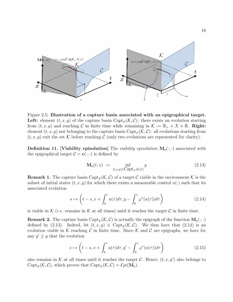
Figure 2.5: Illustration of a capture basin associated with an epigraphical target.Left: element (t, x, y) of the capture basin CaptF (K, C): there exists an evolution startingfrom (t, x, y) and reaching C in finite time while remaining in K := R+ × X × R. Right:element (t, x, y) not belonging to the capture basin CaptF (K, C): all evolutions starting from(t, x, y) exit the set K before reaching C (only two evolutions are represented for clarity).

Definition 11. [Viability episolution] The viability episolution Mc(·, ·) associated withthe epigraphical target C = c(·, ·) is defined by

Mc(t, x) := inf(t,x,y)∈CaptF (K,C)

y (2.13)

Remark 1. The capture basin CaptF (K, C) of a target C viable in the environment K is thesubset of initial states (t, x, y) for which there exists a measurable control u(·) such that itsassociated evolution

s 7→(t− s, x+

∫ s

0

u(τ)dτ, y −∫ s

0

ϕ∗(u(τ))dτ

)(2.14)

is viable in K (i.e. remains in K at all times) until it reaches the target C in finite time.

Remark 2. The capture basin CaptF (K, C) is actually the epigraph of the function Mc(·, ·)defined by (2.13). Indeed, let (t, x, y) ∈ CaptF (K, C). We thus have that (2.14) is anevolution viable in K reaching C in finite time. Since K and C are epigraphs, we have forany y′ ≥ y that the evolution

s 7→(t− s, x+

∫ s

0

u(τ)dτ, y′ −∫ s

0

ϕ∗(u(τ))dτ

)(2.15)

also remains in K at all times until it reaches the target C. Hence, (t, x, y′) also belongs toCaptF (K, C), which proves that CaptF (K, C) = Epi(Mc).

19

We illustrate the viability episolution associated with a given value condition in Fig-ure 2.6.

Figure 2.6: Illustration of a viability episolution.We represent on the same figure a target C and its associated viability episolution Mc(·, ·).The episolution is the lower boundary of the capture basin CaptF (K, C), shaded in this figure.

The viability episolution Mc(·, ·) defined by equation (2.13) is shown in theorem 1 to bea B-J/F solution to equation (2.5). If furthermore Mc(·, ·) is differentiable, it is a classicalsolution to equation (2.5).

The work [8] defines the B/J-F solution in hypographical form for a function N(·, ·)satisfying an inhomogeneous HJ PDE:

∂N(t, x)

∂t+ ψ

(∂N(t, x)

∂x

)= ψ(v(t)) (2.16)

The following theorem is identical to the main existence and uniqueness theorem of [8]modulo the variable change M(t, x) = −N(t, x)+

∫ t0ψ(v(u))du, the translation of hypographs

into epigraphs and the corresponding change on epi/hypo derivatives and differentials.

Theorem 1. [Barron-Jensen/Frankowska solution] [8] For any lower semicontinuousvalue condition ci, the associated solution Mci is the unique lower semicontinuous functionlower than ci satisfying:

{(i) ∀(t, x) ∈ Dom(Mci)\Dom(ci), ∀(pt, px) ∈ d−Mci(t, x), pt − ψ(−px) = 0(ii) ∀(t, x) ∈ Dom(Mci)\Dom(ci), ∀(pt, px) ∈ (Dom(D↑Mci(t, x)))+, pt − σ(Dom(ϕ∗), px) = 0

(2.17)

where the epiderivative D↑ is defined by its epigraph:

Ep(D↑Mci(t, x)) := TEp(Mci )(t, x,Mci(t, x)) (2.18)

20

where in the formulae (2.18) and (2.17) TZ(z) represents the contingent cone to Z at z(see [10]), σ(·, ·) is the support function (see [6, 10, 9]), the + superscript denotes the normalcone (see [8]) and where the subdifferential d− of a function u : X → R ∪ {+∞} is definedby d−u(x) = {p ∈ X∗|∀v ∈ X, 〈p, v〉 ≤ D↑u(x)(v)}.

Theorem 1 ensures that Mci is a solution to the HJ PDE (2.5) in the B-J/F sense. In

particular, since d−Mci(t, x) = {(∂Mci (t,x)

∂t,∂Mci (t,x)

∂x)} whenever Mci(t, x) is differentiable,

equation (2.17) implies the following property:

∀(t, x) ∈ Dom(Mci)\Dom(ci) such that Mci is differentiable,∂Mci (t,x)

∂t− ψ

(−∂Mci (t,x)

∂x

)= 0

(2.19)The construction of the B-J/F solution to (2.5) as a capture basin enables the definition

of a Lax-Hopf formula.

2.3.3 The Lax-Hopf formula

The viability episolution Mc(·, ·) associated with a general value condition c(·, ·) can becomputed using the following generalized Lax-Hopf formula. The classical Lax-Hopf formulaecan be found in [8] for initial and upstream boundary conditions.

Theorem 2. [Generalized Lax Hopf formula] The viability episolution Mc(·, ·) associ-ated with a target C := Epi(c), for a given lower semicontinuous function c(·, ·) and definedby equation (2.13) can be expressed as:

Mc(t, x) = inf(u,T )∈Dom(ϕ∗)×R+

(c(t− T, x+ Tu) + Tϕ∗(u)) (2.20)

Proof — We fix (t, x) ∈ R+ × X and define R as the set of elements (u(·), T, y)belonging to L1(0,∞; Dom(ϕ∗))× R+ × R and satisfying viability property (2.21):

∀s ∈ [0, T ]

(t− s, x+

∫ s

0

u(τ)dτ, y −∫ s

0

ϕ∗(u(τ))dτ

)∈ K (2.21)

Equations (2.13) and (2.14) thus imply the following formula:

Mc(t, x) = inf(u(·),T,y)∈R such that (t−T,x+

∫ T0 u(τ)dτ,y−

∫ T0 ϕ∗(u(τ))dτ)∈Epi(c)

y (2.22)

Since the graph of the value condition c(·, ·) (denoted Graph(c)) is the lower boundaryof Epi(c), we have that(

t− T, x+∫ T0u(τ)dτ, y −

∫ T0ϕ∗(u(τ))dτ

)∈ Epi(c)

and(t− T, x+

∫ T0u(τ)dτ, z −


)∈ Graph(c)

}⇒ z ≤ y (2.23)

21

Hence, we can (without any further assumption) write equation (2.22) as:

Mc(t, x) = inf(u(·),T,y)∈R such that (t−T,x+

∫ T0 u(τ)dτ,y−

∫ T0 ϕ∗(u(τ))dτ)∈Graph(c)

y (2.24)

Since c is infinite outside of its domain of definition and given the definition of Graph(c),equation (2.24) can be expressed as follows:

Mc(t, x) = inf(u(·),T,y)∈R

[c

(t− T, x+

∫ T

0

u(τ)dτ

)+

∫ T

0

ϕ∗(u(τ))dτ

](2.25)

We consider a fixed element (u(·), T, y) ∈ R and define the following constant controlfunction u on the time interval [0, T ] as:

u :=1

T

∫ T

0

u(τ)dτ (2.26)

The control function u is the average value of the control function u(·) on the time interval[0, T ]. Note that by convexity of K, (u, T, y) ∈ R if (u(·), T, y) ∈ R. In the following, weslightly abuse the notation by calling u(·) the constant function t→ u.

We define y(u(·), T ) and y(u(·), T ) respectively as the values of the term minimizedin (2.25) obtained for the control functions u(·) and u(·) and for the capture time T :{

y(u(·), T ) = c(t− T, x+∫ T0u(τ)dτ) +


y(u(·), T ) = c(t− T, x+ T u) + Tϕ∗(u)(2.27)

Since ϕ∗ is convex and lower semicontinuous, Jensen’s inequality implies

ϕ∗(

1

T

∫ T

0

u(τ)dτ

)≤ 1

T

∫ T

0

ϕ∗(u(τ))dτ (2.28)

and thus, since uT =∫ T0u(τ)dτ

y(u(·), T ) ≤ y(u(·), T ) (2.29)

Equation (2.29) thus implies that one can replace the search of the infimum over the classof measurable functions u(·) by the search of the infimum over the set of constant functionsu(·).

Hence, we can write equation (2.25) as:

Mc(t, x) = inf(u,T )∈Dom(ϕ∗)×R+

(c(t− T, x+ Tu) + Tϕ∗(u)) (2.30)

which enables us to restrict ourselves to the set of constant controls and completes theproof. �

22

Remark 3. Given a constant control function u, the coefficient T used for the minimiza-tion in equation (2.20) can be restricted to the elements of the set Sc(t, x, u) defined byformula (2.31):

Sc(t, x, u) := {s ∈ R+ such that (t− s, x+ su) ∈ Dom(c)} (2.31)

Indeed, when T /∈ Sc(t, x, u), c(t− T, x+ Tu) is infinite.

We could also alternatively define for any (t, x) the set Rc(t, x) as Rc(t, x) := {(u, T ) ∈Dom(ϕ∗) × R+ s. t. (t − T, x + Tu) ∈ Dom(c)}. Note that the coefficients (u, T ) usedfor the minimization in equation (2.20) can also be restricted to the elements of Rc (when(u, T ) /∈ Rc(t, x), c(t− T, x+ Tu) is infinite).

Remark 4. When ∀u ∈ Dom(ϕ∗), Sc(t, x, u) = ∅, equation (2.30) involves a minimizationon an empty set and Mc(t, x) is infinite.

Remark 5. Since c(t − T, x + Tu) = +∞ when (t − T, x + Tu) /∈ Dom(c), we can writeequation (2.30) as:

Mc(t, x) = inf{(u,T )∈Dom(ϕ∗)×R+ such that T∈Sc(t,x,u)}

(c(t− T, x+ Tu) + Tϕ∗(u)) (2.32)

or alternatively as:

Mc(t, x) = inf{(u,T )∈Rc(t,x)}

(c(t− T, x+ Tu) + Tϕ∗(u)) (2.33)

Specific forms of the Lax-Hopf formula (2.20) associated with affine initial, boundary andinternal conditions are presented in section 2.5.

2.4 Properties of the Barron-Jensen/Frankowska solu-

tions to Hamilton-Jacobi equations

2.4.1 Domain of definition

Proposition 1. [Domain of definition] For a given value condition c(·, ·), the domain ofdefinition of Mc(·, ·), also called domain of influence of c(·, ·), is defined by the followingformula:

Dom(Mc) =⋃

(t,x)∈Dom(c)

⋃T∈R+

{t+ T} × [x− ν]T, x+ ν[T ]

(2.34)

23

Proof — The generalized Lax Hopf formula (2.20) implies that

Dom(Mc) = {(t, x) ∈ R+ ×X such that ∃(T, u) ∈ R+ ×Dom(ϕ∗)and (t− T, x+ Tu) ∈ Dom(c)}

Equation (2.34) is derived from the previous formula, observing that u ranges in Dom(ϕ∗) :=[−ν[, ν]]. �

Remark 6. The domain of influence of c(·, ·) is the union of the cones originating at (t, x) ∈Dom(c) and limited by the minimal −ν[ and maximal ν] slopes of the Hamiltonian. Thisproperty is illustrated in Figure 2.7.

Figure 2.7: Illustration of the domain of influence of a value condition.We define a value condition c(·) on a domain represented by two black segments at t = 0.The domain of influence of c(·, ·) is highlighted in gray.

24

Figure 2.8: Illustration of the inf-morphism property.Top: representation of the target C1 := Epi(c1) (left), representation of the correspondingepisolution M1(·, ·) (right). Center: representation of the target C2 := Epi(c2) (left),representation of the corresponding episolution M2(·, ·) (right). Bottom: Representationof the target C := C1

⋃C2 (left). The episolution M(·, ·) associated with the target C (right)

is the minimum of the episolutions M1(·, ·) and M2(·, ·) associated with C1 and C2.

2.4.2 The inf-morphism property

It is well known [6, 7, 8] that for a given environment K, the capture basin of a finiteunion of targets is the union of the capture basins of these targets.

25

CaptF

(K,⋃i∈I

Ci

)=⋃i∈I

CaptF (K, Ci) (2.35)

This property can be translated in epigraphical form as follows.

Proposition 2. [Inf-morphism property] [8] Let ci (i belongs to a finite set I) be afamily of functions whose epigraphs are the targets Ci. Since the epigraph of the minimumof the functions ci is the union of the epigraphs of the functions ci, the target C :=

⋃i∈I Ci

is the epigraph of the function c := mini∈I ci. Hence, equation (2.35) implies the followingproperty, known as inf-morphism property :

∀ t ≥ 0, x ∈ X, Mc(t, x) = mini∈I

Mci(t, x) (2.36)

Remark 7. The inf-morphism property enables us to decompose a complex problem intomore tractable subproblems. For instance, a piecewise affine initial condition can be decom-posed as the minimum of a finite number of affine initial conditions. Hence, the solutionassociated with a piecewise affine initial condition is the minimum of a finite number ofsolutions associated with affine initial conditions.

The inf-morphism property is illustrated in Figure 2.8.Note that in the context of traffic flow engineering, this property was identified but not

proved mathematically by Newell in [80].

2.4.3 Convexity property of the solutions associated with convexvalue conditions

We now show an important convexity property of the solution to (2.5) associated withconvex value conditions. Let a convex value condition c(·, ·) be defined defined on a compactand nonempty domain Dom(c) ⊂ [0, tmax] × X. Since c(·, ·) is convex and defined on acompact set, it is bounded below. In order to prove the convexity of the solution Mc(·, ·)associated with c(·, ·), we first need to define a variable change as follows.

Definition 12. [Variable change for the auxiliary control] We define a new variablev as v = Tu and define the cone D :=

{[−ν[t, ν]t]× {t} | t ∈ R+

}.

Note that definition 12 implies that (u, T ) ∈ Dom(ϕ∗)×R+ if and only if (v, T ) ∈ D. Wenow define an auxiliary objective function f(·, ·, ·, ·), which is the argument of the Lax-Hopfformula (2.20) with the variable change v = Tu.

Definition 13. [Auxiliary objective function] We define the function f(·, ·, ·, ·) as:

∀(t, x, v, T ) ∈ R+ ×X ×D,f(t, x, v, T ) := c(t− T, x+ v) + Tϕ∗

(vT

)

26

Note that f(·, ·, ·, ·) is bounded below since the value condition c(·, ·) is bounded belowand the function ϕ∗(·) is positive. By definition of f(·, ·, ·, ·), we can rewrite equation (2.20)as:

Mc(t, x) = inf(v,T )∈D

f(t, x, v, T ) (2.37)

Equation (2.37) implies:

Epi(Mc) = {(t, x, y) | ∃(v, T ) ∈ D s.t. (t, x, v, T, y) ∈ Epi(f)} (2.38)

The above variable change enables us to prove the following convexity property.

Proposition 3. [Convexity property of solutions associated with convex valueconditions] The solution Mc(·, ·) associated with a convex value condition c(·, ·) is convex.

Proof — Since ϕ∗(·) is convex, its associated perspective function (v, T )→ Tϕ∗( vT

) isalso convex [18] for T > 0. Since the function (t, x, v, T )→ (t− T, x+ v) is affine and c(·, ·)is convex, the function (t, x, v, T ) → c(t − T, x + v) is convex [87, 18]. Hence the functionf(·, ·, ·, ·) is convex as the sum of two convex functions.

Since the function f(·, ·, ·, ·) is convex, its epigraph Epi(f) is also convex. Since theset Epi(c) is nonempty, the epigraph of Mc(·, ·) is nonempty by the inclusion Epi(c) ⊂CaptF (K, Epi(c)) := Epi(Mc) (see [6] for a proof of this property).

Hence, equation (2.38) implies that the epigraph of Mc is convex, since it is the projectionof a convex set on a subspace [87, 18]. �

In particular, proposition 3 implies that the solutions associated with affine initial, bound-ary and internal conditions are convex. We now prove that they can also be computedexplicitly for general concave Hamiltonians.

27

2.5 Analytic solutions associated with affine initial, bound-

ary and internal conditions

In this section, we compute the solutions associated with affine initial, boundary andinternal conditions analytically. For each type of value condition, we follow the procedureoutlined below.

1. Write the Lax-Hopf formula associated with the corresponding affine value condition.Because of the structure of the affine value condition, we can compute the set Sc(t, x, u)defined by (2.31) explicitly, which enables us to express (2.32) as a minimization overa single variable.

2. Write the minimization problem associated with this instantiation of the Lax-Hopfformula as a convex optimization problem (convex objective and convex constraints).

3. Analytically find a minimizer of the convex optimization problem, using subderiva-tives (2.10).

2.5.1 Analytic Lax-Hopf formula associated with an affine initialcondition

Definition 14. [Affine initial condition] We consider the following affine initial conditionM0,i(0, x), where i is an integer:

M0,i(0, x) =

{aix+ bi if x ∈ [αi, αi+1]+∞ otherwise

(2.39)

The following formula expresses the Lax-Hopf formula (2.20) for the specific initial con-dition (2.39).

Proposition 4. [Lax-Hopf formula for an affine initial condition] The Lax-Hopfformula associated with the initial condition (2.39) can be expressed as:

MM0,i(t, x) = inf

u∈Dom(ϕ∗)∩[αi−xt

,αi+1−x

t

] (ai(x+ tu) + bi + tϕ∗(u)) , ∀(t, x) ∈ R∗+ ×X

(2.40)and

∀x×X, MM0,i(0, x) = inf

(T,u)∈Dom(ϕ∗)×[0,0](ai(x+ 0u) + bi + 0ϕ∗(u)) = aix+ bi (2.41)

28

Proof — The Lax-Hopf formula associated with an initial condition reads:

MM0,i(t, x) = inf

(T,u)∈Dom(ϕ∗)×[0,t] such that (x+Tu)∈[αi,αi+1] and t−T=0

(ai(x+ tu) + bi + Tϕ∗(u))

(2.42)This formula is valid for all (t, x) ∈ R+×X. Since t−T = 0, we have T = t. Since t > 0,

the condition (x + tu) ∈ [αi, αi+1] is equivalent to u ∈ [αi−xt, αi+1−x

t], which in turn implies

equation (2.40). �The domain of definition of the solution can be explicitly characterized as follows.

Proposition 5. [Domain of influence of an affine initial condition] The domain ofdefinition of MM0,i

(·, ·) is given by the following formula:

Dom(MM0,i) =

{(t, x) ∈ R∗+ ×Xsuch that αi − ν]t ≤ x ≤ αi+1 + ν[t

}(2.43)

Proof — The Lax-Hopf formula (2.40) implies:

Dom(MM0,i) :=

{(t, x) ∈ R∗+ ×Xsuch that ∃u ∈ Dom(ϕ∗) ∩

[αi−xt, αi+1−x

t

]}Equation (2.43) is obtained using the above formula and noting that Dom(ϕ∗) = [−ν[, ν]].�

The solution can be computed analytically by minimizing an auxiliary function, whichwe now define.

Definition 15. [Auxiliary objective function] For all (ai, bi, t, x) ∈ R2 × Dom(MM0,i),

we define an objective function ζai,bi,t,x(·) by the following formula:

∀u ∈ Dom(ϕ∗), ζai,bi,t,x(u) := ai(x+ tu) + bi + tϕ∗(u) (2.44)

Given this definition, equation (2.40) becomes:

∀(t, x) ∈ R∗+ ×X, MM0,i(t, x) = inf

u∈Dom(ϕ∗)∩[αi−xt

,αi+1−x

t

]ζai,bi,t,x(u)(2.45)

The function ζai,bi,t,x(·) is convex as the sum of two convex functions and thus subdiffer-entiable on Dom(ϕ∗) in the sense of (2.10). The subderivative of ζai,bi,t,x(·) is given by:

∀u ∈ Dom(ϕ∗), ∂−ζai,bi,t,x(u) = {w | ∃v ∈ ∂−ϕ∗(u), w = ait+ vt}:= t · ({ai}+ ∂−ϕ

∗(u))(2.46)

with a slight abuse of notation for the summation of the two sets in the second equality.This last expression can now be used to analytically compute the minimizer.

29

Proposition 6. [Explicit minimization of ζai,bi,t,x(·)] We now assume that ai in thevalue condition M0,i given by (2.39) satisfies the condition −ai ∈ Dom(ψ) := [0, ω]. Sinceψ(·) is concave, it is also superdifferentiable on its domain of definition and thus ∀ρ ∈[0, ω], ∂+ψ(ρ) 6= ∅.

Let u0(ai) be an element of −∂+ψ(−ai) 6= ∅. Note that the Legendre-Fenchel inversionformula (2.9) implies that u0(ai) ∈ Dom(ϕ∗) and −ai ∈ ∂−ϕ∗(u0(ai)). Using this definitionof u0(ai), the function ζai,bi,t,x(·) has the following minimizer over Dom(ϕ∗) ∩ [αi−x

t, αi+1−x

t]:

u = u0(ai) if u0(ai) ∈ [αi−xt, αi+1−x

t]

u = αi−xt

if u0(ai) ≤ αi−xt

u = αi+1−xt

if u0(ai) ≥ αi+1−xt

(2.47)

Proof — The function ζai,bi,t,x(u) is minimal for a given u ∈ Dom(ϕ∗) if and only if 0 ∈∂−ζai,bi,t,x(u) by [18]. By equation (2.46), this happens if and only if for this u, −ai ∈ ∂−ϕ∗(u).Using the Legendre-Fenchel inversion formula (2.9), we can rewrite u := u0(ai) ∈ −∂+ψ(−ai)as −ai ∈ ∂−ϕ

∗(u0(ai)) and thus u0(ai) minimizes ζai,bi,t,x(·) over Dom(ϕ∗). Hence, sinceζai,bi,t,x(·) is convex, ζai,bi,t,x(u) is decreasing for u ≤ u0(ai) and increasing for u ≥ u0(ai),which implies equation (2.47). �

Proposition 7. [Computation of MM0,i(·, ·)] Let u0(ai) be defined as in proposition 6.

For all (t, x) ∈ Dom(MM0,i), the expression MM0,i

(t, x) can be computed using the followingformula:

MM0,i(t, x) =

(i) tψ(−ai) + aix+ biif u0(ai) ∈ [αi−x

t, αi+1−x

t]

(ii) aiαi + bi + tϕ∗(αi−xt

)if u0(ai) ≤ αi−x

t

(iii) aiαi+1 + bi + tϕ∗(αi+1−xt

)

if u0(ai) ≥ αi+1−xt

(2.48)

Proof — The cases (ii) and (iii) of equation (2.48) are trivially obtained by combiningequations (2.40) and (2.47). Since the function −ψ(·) is convex, it is identical [18] to itsFenchel biconjugate:

∀ρ ∈ [0, ω], ψ(ρ) = infu∈Dom(ϕ∗)

(−ρu+ ϕ∗(u))

The function g : u → aiu + ϕ∗(u) is convex and thus subdifferentiable on Dom(ϕ∗).By definition of u0(ai), 0 ∈ ∂−g(u0(ai)). This last property implies that u0(ai) minimizesg(·) over Dom(ϕ∗) and thus that ψ(−ai) = aiu0(ai) + ϕ∗(u0(ai)). Hence, the case (i) ofequation (2.48) is obtained by combining equations (2.40), (2.47) and the property ψ(−ai) =aiu0(ai) + ϕ∗(u0(ai)). �

30

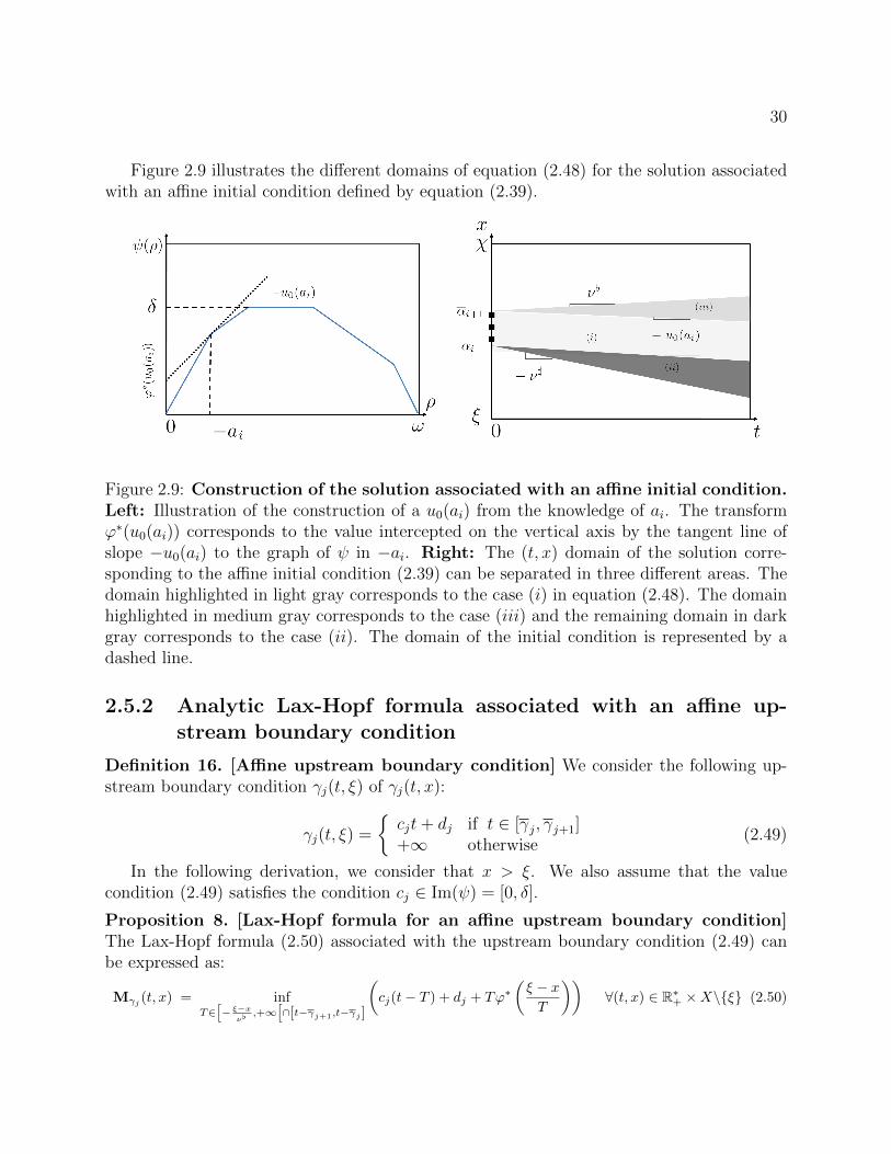
Figure 2.9 illustrates the different domains of equation (2.48) for the solution associatedwith an affine initial condition defined by equation (2.39).

Figure 2.9: Construction of the solution associated with an affine initial condition.Left: Illustration of the construction of a u0(ai) from the knowledge of ai. The transformϕ∗(u0(ai)) corresponds to the value intercepted on the vertical axis by the tangent line ofslope −u0(ai) to the graph of ψ in −ai. Right: The (t, x) domain of the solution corre-sponding to the affine initial condition (2.39) can be separated in three different areas. Thedomain highlighted in light gray corresponds to the case (i) in equation (2.48). The domainhighlighted in medium gray corresponds to the case (iii) and the remaining domain in darkgray corresponds to the case (ii). The domain of the initial condition is represented by adashed line.

2.5.2 Analytic Lax-Hopf formula associated with an affine up-stream boundary condition

Definition 16. [Affine upstream boundary condition] We consider the following up-stream boundary condition γj(t, ξ) of γj(t, x):

γj(t, ξ) =

{cjt+ dj if t ∈ [γj, γj+1]+∞ otherwise

(2.49)

In the following derivation, we consider that x > ξ. We also assume that the valuecondition (2.49) satisfies the condition cj ∈ Im(ψ) = [0, δ].

Proposition 8. [Lax-Hopf formula for an affine upstream boundary condition]The Lax-Hopf formula (2.50) associated with the upstream boundary condition (2.49) canbe expressed as:

Mγj (t, x) = infT∈

[− ξ−x

ν[,+∞

[∩[t−γj+1,t−γj]

(cj(t− T ) + dj + Tϕ∗

(ξ − xT

))∀(t, x) ∈ R∗+ ×X\{ξ} (2.50)

31

Proof — The Lax-Hopf formula (2.32) associated with the upstream boundary condi-tion reads:

Mγj(t, x) = inf(u,T )∈Dom(ϕ∗)×R+ such that x+Tu=ξ and γj≤t−T≤γj+1

(cj(t− T ) + dj + Tϕ∗(u))

(2.51)We define the variable change T := ξ−x

u> 0, which represents the capture time using

the control u (see [31]). Since T = ξ−xu

> 0 and x > ξ, we have u < 0. The constraint

u ∈ Dom(ϕ∗) := [−ν[, ν]] thus implies T ∈ [− ξ−xν[,+∞[. The additional constraint t− ξ−x

u∈

[γj, γj+1] results from the definition of γj(·, ·) and implies T ∈ [t− γj+1, t− γj], which yieldsequation (2.50). �

Proposition 9. [Domain of influence of an affine upstream boundary condition]The domain of definition of Mγj(·, ·) is given by the following formula:

Dom(Mγj) ={

(t, x) ∈ R+ ×X such that x ≤ ξ + ν[(t− γj)}

(2.52)


Dom(Mγj) :=

{(t, x) ∈ R+ ×X such that ∃T ∈

[−ξ − x

ν[,+∞

[∩[t− γj+1, t− γj

]}Hence, (t, x) ∈ Dom(Mγj) if and only if − ξ−x

ν[≤ t − γj, which in turn implies equation

(2.52). �

Definition 17. [Auxiliary objective function] For all (t, x) ∈ Dom(Mγj), we define anobjective function ηcj ,dj ,t,x(·) by the following formula:

∀T ∈ R∗+ ηcj ,dj ,t,x(T ) := cj(t− T ) + dj + Tϕ∗(ξ − xT

)(2.53)


Mγj(t, x) =inf

T∈[− ξ−x

ν[,+∞


ηcj ,dj ,t,x(T )(2.54)

Since ϕ∗(·) is convex, its associated perspective function T → Tϕ∗( ξ−xT

) is also convex [18]for T > 0. Hence the function ηcj ,dj ,t,x(·) is convex as the sum of two convex functions. Thesubderivative of ηcj ,dj ,t,x(·) is given by:

∀T ∈ [− ξ−xν[,+∞[, ∂−ηcj ,dj ,t,x(T ) =

{w | ∃v ∈ ∂−ϕ∗( ξ−xT ), w = −cj + ϕ∗( ξ−x

T)− ξ−x

Tv}

:={−cj + ϕ∗( ξ−x

T)}− ξ−x

T∂−ϕ

∗( ξ−xT

)(2.55)

with a slight abuse of notation for the second line as previously.

32

Definition 18. [Density associated with cj] Recalling that Im (ψ) := [0, δ], we define ρcas:

ρc = infρ∈[0,ω] such that ψ(ρ)=δ

ρ

Since cj ∈ Im(ψ) = [0, δ], there exists ρj ∈ [0, ρc] such that ψ(ρj) = cj. Note that sinceψ(·) is concave and δ > 0, ψ(·) is increasing on [0, ρc] and thus ∂+ψ(ρj) ∩ R+ 6= ∅.

• Let u0(ρj) be an element of −∂+ψ(ρj) ∩ R− 6= ∅.

• Let T0(ρj, x) be defined as

T0(ρj, x) :=

{ ξ−xu0(ρj)

if u0(ρj) 6= 0

+∞ if u0(ρj) = 0(2.56)

We have by the Legendre-Fenchel inversion formula that u0(ρj) ∈ Dom(ϕ∗) and ρj ∈∂−ϕ

∗(u0(ρj)).

Proposition 10. [Explicit minimization of ηcj ,dj ,t,x(·)] Let T0(ρj, x) be given by defini-tion 18. For all (t, x) ∈ Dom(Mγj), the function ηcj ,dj ,t,x(·) has the following minimizer over

[− ξ−xν[,∞[∩[t− γj+1, t− γj]:

T0(ρj, x) if T0(ρj, x) ∈ [t− γj+1, t− γj]t− γj if t− γj ≤ T0(ρj, x)t− γj+1 if T0(ρj, x) ≤ t− γj+1

(2.57)

Proof — The function ηcj ,dj ,t,x(·) is minimal for a given T > 0 if and only if 0 ∈∂−ηcj ,dj ,t,x(T ) by [18]. Since u0(ρj) ∈ −∂+ψ(ρj)∩R−, we have by the Legendre-Fenchel inver-sion formula that ρj ∈ ∂−ϕ∗(u0(ρj)). This last formula implies 0 ∈ ∂− (ϕ∗(·)− ·ρj) (u0(ρj))and thus that:

ψ(ρj) = infu∈Dom(ϕ∗)

[ϕ∗(u)− ρju] = ϕ∗(u0(ρj))− ρju0(ρj)

The property cj = ψ(ρj) implies that −cj + ϕ∗ (u0(ρj)) = ρju0(ρj) by the previous formula.Equation (2.55) thus implies:

∂−ηcj ,dj ,t,x(ξ−xu0(ρj)

) = {w | ∃v ∈ ∂−ϕ∗ (u0(ρj)) , w = ρju0(ρj)− u0(ρj)v}:= {ρju0(ρj)} − u0(ρj)∂−ϕ∗ (u0(ρj))

(2.58)

Since ρj ∈ ∂−ϕ∗ (u0(ρj)), this last property implies that 0 ∈ ∂−ηcj ,dj ,t,x(

ξ−xu0(ρj)

). Hence,

T0(ρj, x) := ξ−xu0(ρj)

minimizes the convex function ηcj ,dj ,t,x(·) over R∗+.

33

Since ηcj ,dj ,t,x(·) is convex, it is decreasing for T ≤ T0(ρj, x) and increasing for T ≥T0(ρj, x). The values of the capture time T which minimize ηcj ,dj ,t,x(T ) over [− ξ−x

ν[,∞[∩[t−

γj+1, t − γj] are thus given by equation (2.57). Note that the property u0(ρj) ∈ [−ν[, 0]

implies − ξ−xν[≤ T0(ρj, x). Note also that since (t, x) ∈ Dom(Mγj), we have − ξ−x

ν[≤ t − γj.

�

Proposition 11. [Computation of Mγj(·, ·)] For all (t, x) ∈ Dom(Mγj), the solutionMγj(t, x) can be computed using the following formula:

Mγj(t, x) =

(i) tψ(ρj) + ρj(ξ − x) + dj if T0(ρj, x) ∈ [t− γj+1, t− γj](ii) ψ(ρj)γj + dj + (t− γj)ϕ∗( ξ−xt−γj

) if t− γj ≤ T0(ρj, x)

(iii) ψ(ρj)γj+1 + dj + (t− γj+1)ϕ∗( ξ−xt−γj+1

) if T0(ρj, x) ≤ t− γj+1

(2.59)

Proof — The cases (ii) and (iii) in equation (2.59) are trivially obtained by combiningequations (2.54) and (2.57). The case (i) in equation (2.59) is obtained by combining (2.53),

(2.57) and observing that ϕ∗(

ξ−xT0(ρj ,x)

)= ψ(ρj) + ξ−x

T0(ρj ,x)ρj. �

Remark 8. Equation (2.59) can also be obtained from equation (2.83), observing that theaffine upstream boundary condition (2.49) can be viewed as an affine internal condition ofthe form (2.73), where:

δl = γjδl+1 = γj+1

xl = ξvl = 0gl = cjhl = cjγj + dj

(2.60)

Figure 2.10 illustrates the different domains of equation (2.59) for the solution associatedwith an affine upstream condition defined by equation (2.49).

34

Figure 2.10: Construction of the solution associated with an affine upstreamboundary condition.Left: Illustration of the construction of a u0(ρj) from a known cj. The transform ϕ∗(u0(ρj))corresponds to the value intercepted on the vertical axis by the tangent line of slope −u0(ρj)to the graph of ψ in ρj. Right: The (t, x) domain of the solution corresponding to theaffine upstream boundary condition (2.49) can be separated in three different areas. Thedomain highlighted in light gray corresponds to the case (i) in equation (2.59). The domainhighlighted in dark gray corresponds to the case (ii) and the remaining domain in mediumgray corresponds to the case (iii). The domain of the upstream boundary condition isrepresented by a dashed line.

2.5.3 Analytic Lax-Hopf formula associated with an affine down-stream boundary condition

Definition 19. [Affine downstream boundary condition] We consider the followingdownstream boundary condition βk(t, χ) of β(t, x):

βk(t, x) =

{ekt+ fk if t ∈ [βk, βk+1]+∞ otherwise

(2.61)

In the following computation, we consider that x < χ. We also assume that the valuecondition (2.61) satisfies the condition ek ∈ Im(ψ) = [0, δ].

Proposition 12. [Lax-Hopf formula for an affine downstream boundary condition]The Lax-Hopf formula (2.62) associated with the downstream boundary condition (2.61) can

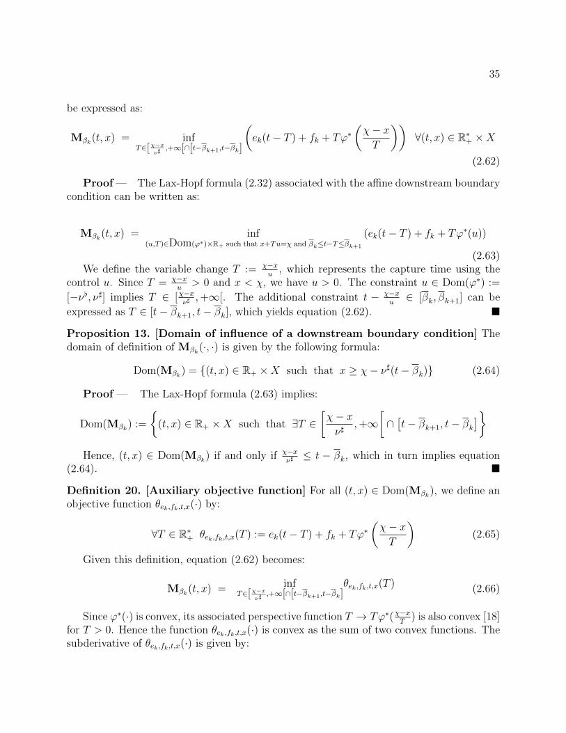
35

be expressed as:

Mβk(t, x) = infT∈[χ−x

ν],+∞[∩[t−βk+1,t−βk]

(ek(t− T ) + fk + Tϕ∗

(χ− xT

))∀(t, x) ∈ R∗+ ×X

(2.62)

Proof — The Lax-Hopf formula (2.32) associated with the affine downstream boundarycondition can be written as:

Mβk(t, x) = inf(u,T )∈Dom(ϕ∗)×R+ such that x+Tu=χ and βk≤t−T≤βk+1

(ek(t− T ) + fk + Tϕ∗(u))

(2.63)We define the variable change T := χ−x

u, which represents the capture time using the

control u. Since T = χ−xu

> 0 and x < χ, we have u > 0. The constraint u ∈ Dom(ϕ∗) :=

[−ν[, ν]] implies T ∈ [χ−xν],+∞[. The additional constraint t − χ−x

u∈ [βk, βk+1] can be

expressed as T ∈ [t− βk+1, t− βk], which yields equation (2.62). �

Proposition 13. [Domain of influence of a downstream boundary condition] Thedomain of definition of Mβk(·, ·) is given by the following formula:

Dom(Mβk) = {(t, x) ∈ R+ ×X such that x ≥ χ− ν](t− βk)} (2.64)


Dom(Mβk) :=

{(t, x) ∈ R+ ×X such that ∃T ∈

[χ− xν]

,+∞[∩[t− βk+1, t− βk

]}Hence, (t, x) ∈ Dom(Mβk) if and only if χ−x

ν]≤ t − βk, which in turn implies equation

(2.64). �

Definition 20. [Auxiliary objective function] For all (t, x) ∈ Dom(Mβk), we define anobjective function θek,fk,t,x(·) by:

∀T ∈ R∗+ θek,fk,t,x(T ) := ek(t− T ) + fk + Tϕ∗(χ− xT

)(2.65)



ν],+∞[∩[t−βk+1,t−βk]

θek,fk,t,x(T ) (2.66)

Since ϕ∗(·) is convex, its associated perspective function T → Tϕ∗(χ−xT

) is also convex [18]for T > 0. Hence the function θek,fk,t,x(·) is convex as the sum of two convex functions. Thesubderivative of θek,fk,t,x(·) is given by:

36

∀T ∈ [χ−xν],+∞[, ∂−θek,fk,t,x(T ) =

{w | ∃v ∈ ∂−ϕ∗(χ−xT ), w = −ek + ϕ∗(χ−x

T)− χ−x

Tv}

:={−ek + ϕ∗(χ−x

T)}− χ−x

T∂−ϕ

∗(χ−xT

)(2.67)

with a slight abuse of notation for the second line as in the previous two sections.

Definition 21. [Density associated with ek] Recalling that Im(ψ) = [0, δ], we define ρcas:

ρc = supρ∈[0,ω] such that ψ(ρ)=δ

ρ

Since ek ∈ Im(ψ) = [0, δ], there exists ρk ∈ [ρc, ω] such that ψ(ρk) = ek. Note that since ψ(·)is concave and δ > 0, ψ(·) is decreasing on [ρc, ω] and thus ∂+ψ(ρk) ∩ R− 6= ∅.

• Let u0(ρk) be an element of −∂+ψ(ρk) ∩ R+

• Let T0(ρk, x) be defined as

T0(ρk, x) :=

{ ξ−xu0(ρk)

if u0(ρk) 6= 0

+∞ if u0(ρk) = 0(2.68)

We have by the Legendre-Fenchel inversion formula that ρk ∈ ∂−ϕ∗(u0(ρk)), which impliesthat u0(ρk) ∈ Dom(ϕ∗).

Remark 9. Note that the definition of ρc differs from the previous section for functions ψ(·)which are not strictly concave. This is sometimes referred as “lower critical density” (section2.5.2) and “upper critical density” (section 2.5.3), but we have kept the same notation sincethe two corresponding densities are only intermediate variables in our derivations.

Proposition 14. [Explicit minimization of θek,fk,t,x(·)] For all (t, x) ∈ Dom(Mβk), thefunction θek,fk,t,x(·) has the following minimizer over [χ−x

ν],+∞[∩[t− βk+1, t− βk]:

T0(ρk, x) if T0(ρk, x) ∈ [t− βk+1, t− βk]t− βk if t− βk ≤ T0(ρk, x)

t− βk+1 if T0(ρk, x) ≤ t− βk+1

(2.69)

Proof — The function θek,fk,t,x(·) is minimal for a given T > 0 if and only if 0 ∈∂−θek,fk,t,x(T ) by [18]. Since u0(ρk) ∈ −∂+ψ(ρk), we have by the Legendre-Fenchel inversionformula that ρk ∈ ∂−ϕ

∗(u0(ρk)). In the exact same way as the previous section, this lastformula implies that 0 ∈ ∂− (ϕ∗(·)− ·ρk) (u0(ρk)) and thus that:

ψ(ρk) = infu∈Dom(ϕ∗)

[ϕ∗(u)− ρku] = ϕ∗(u0(ρk))− ρku0(ρk)

37

The property ek = ψ(ρk) implies that −ek + ϕ∗(u0(ρk)) = ρku0(ρk). Equation (2.67) thusimplies:

∂−θek,fk,t,x(χ−xu0(ρk)

) = {w | ∃v ∈ ∂−ϕ∗ (u0(ρk)) , w = ρku0(ρk)− u0(ρk)v}:= {ρku0(ρk)} − u0(ρk)∂−ϕ∗ (u0(ρk))

(2.70)

with the same abuse of notation for the second line.Since ρk ∈ ∂−ϕ∗ (u0(ρk)), this last property implies that 0 ∈ ∂−θek,fk,t,x(

χ−xu0(ρk)

). Hence,

T0(ρk, x) := χ−xu0(ρk)

minimizes the convex function θek,fk,t,x(·) over R∗+.

Since θek,fk,t,x(·) is convex, it is decreasing for T < T0(ρk, x) and increasing for T >T0(ρk, x). The values of the capture time T which minimize θek,fk,t,x(T ) over [χ−x

ν],+∞[∩[t−

βk+1, t−βk] are thus given by equation (2.69). Note that the property u0(ρk) ∈ [0, ν]] impliesχ−xν]≤ T0(ρk, x). Note also that since (t, x) ∈ Dom(Mβk), we have χ−x

ν]≤ t− βk. �

Proposition 15. [Computation of Mβk(·, ·)] For all (t, x) ∈ Dom(Mβk), the expressionMβk(t, x) can be computed using the following formula:

Mβk(t, x) =

(i) tψ(ρk) + ρk(χ− x) + fk if T0(ρk, x) ∈ [t− βk+1, t− βk](ii) ψ(ρk)βk + fk + (t− βk)ϕ∗( χ−xt−βk

) if t− βk ≤ T0(ρk, x)

(iii) ψ(ρk)βk+1 + fk + (t− βk+1)ϕ∗( χ−xt−βk+1

) if T0(ρk, x) ≤ t− βk+1

(2.71)

Proof — The cases (ii) and (iii) in equation (2.71) are trivially obtained by combiningequations (2.66) and (2.69). The case (i) in equation (2.71) is obtained by combining (2.66),

(2.69) and observing that ϕ∗(

χ−xT0(ρk,x)

)= ψ(ρk) + χ−x

T0(ρk,x)ρk. �

Remark 10. Equation (2.71) can be obtained from equation (2.84), observing that the affinedownstream boundary condition (2.61) can be viewed as an affine internal condition of theform (2.73), where:

δl = βkδl+1 = βk+1

xl = χvl = 0gl = ekhl = ekβk + fk

(2.72)

Figure 2.11 illustrates the different domains of equation (2.71) for the solution associatedwith an affine downstream boundary condition defined by equation (2.61).

38

Figure 2.11: Construction of the solution associated with an affine downstreamboundary condition.Left: Illustration of the construction of a u0(ρk) from a known ek. The transform ϕ∗(u0(ρk))corresponds to the value intercepted on the vertical axis by the tangent line of slope −u0(ρk)to the graph of ψ in ρk. Right: The (t, x) domain of the solution corresponding to theaffine downstream boundary condition (2.61) can be separated in three different areas. Thedomain highlighted in light gray corresponds to the case (i) in equation (2.71). The domainhighlighted in dark gray corresponds to the case (ii) and the remaining domain in mediumgray corresponds to the case (iii). The domain of the downstream boundary condition isrepresented by a dashed line.

2.5.4 Analytic Lax-Hopf formula associated with an affine internalcondition

The previous section explained how to compute the solution to affine initial and boundaryconditions. We now treat the problem of internal conditions using a similar approach. Aswill appear in this section, the algebra involved in doing this mathematical construction ismore involved than the previous case.

Definition 22. [Affine internal condition] We consider the following affine internal con-dition µl(·, ·), where l is an integer:

µl(t, x) =

gl(t− δl) + hl if x = xl + vl(t− δl)

and t ∈ [δl, δl+1]+∞ otherwise

(2.73)

For the computation of the corresponding solution Mµl(t, x), we assume that (t, x) satisfyx 6= xl + vl(t − δl). In addition, we assume that the constants gl and vl satisfy 0 ≤ gl ≤ϕ∗(−vl).

39

Proposition 16. [Lax-Hopf formula for affine internal condition] The Lax-Hopf for-mula (2.74) associated with the internal boundary condition (2.73) can be expressed as:

Mµl(t, x) = infT∈R+∩[t−δl+1,t−δl]

(gl(t− T − δl) + hl + Tϕ∗

(xl + vl(t− δl − T )− x

T

))(2.74)

Proof — The Lax-Hopf formula (2.32) associated with an affine internal conditionreads:

Mµl(t, x) =

inf(u,T )∈Dom(ϕ∗)×R+ such that x+Tu=xl+vl(t−T−δl) and δl≤t−T≤δl+1

(gl(t− T − δl) + hl + Tϕ∗(u)

)(2.75)

Since x+Tu = xl+vl(t−T −δl), we have u = xl+vl(t−T−δl)−xT

. In addition, the constraint

δl ≤ t− T ≤ δl+1 can be written as T ∈ [t− δl+1, t− δl], which yields (2.74). �The solution to the affine internal condition has a domain of definition, which can be

computed analytically as follows.

Proposition 17. [Domain of influence of an affine internal condition] The domainof definition of Mµl(·, ·) is given by the following formula:

Dom(Mµl) = {(t, x) ∈ R+ ×X such that t ≥ δl and xl − ν](t− δl) ≤ x ≤ xl + ν[(t− δl)}(2.76)


Dom(Mµl) :={

(t, x) ∈ R+ ×X s.t. ∃T ∈ R∗+ ∩ [t− δl+1, t− δl]and xl+vl(t−δl−T )−x

T∈ Dom(ϕ∗)

}Since T > 0, the condition xl+vl(t−δl−T )−x

T∈ Dom(ϕ∗) = [−ν[, ν]] is equivalent to T ≥

xl+vl(t−δl)−xν]+vl

and T ≥ xl+vl(t−δl)−x−ν[+vl

. Hence, (t, x) ∈ Dom(ϕ∗) if and only if the set R∗+ ∩ [t −δl+1, t− δl] ∩ [xl+vl(t−δl)−x

ν]+vl,+∞[∩[xl+vl(t−δl)−x−ν[+vl

,+∞[ is not empty, which implies

max

(0,xl + vl(t− δl)− x

−ν[ + vl,xl + vl(t− δl)− x

ν] + vl

)≤ t− δl

This last inequality implies equation (2.76). �The method followed next also makes use of an auxiliary objective function, which is

later used to explicitly find the minimizer.

40

Definition 23. [Auxiliary objective function] For all (t, x) ∈ Dom(Mµl), we define thefunction κδl,gl,hl,xl,vl,t,x(·) as:

∀T ∈ R∗+, κδl,gl,hl,xl,vl,t,x(T ) :=(gl(t− T − δl) + hl + Tϕ∗

(xl+vl(t−δl−T )−x

T

))(2.77)


Mµl(t, x) = infT∈[max

(0,xl+vl(t−δl)−x−ν[+vl

,xl+vl(t−δl)−x

ν]+vl,t−δl+1

),t−δl

]κδl,gl,hl,xl,vl,t,x(T )(2.78)

Since ϕ∗(·) is convex, the function h : u → ϕ∗(u − vl) is convex and its associated

perspective function T → Th(xl+vl(t−δl)−xT

) is also convex for T > 0 by [18]. Hence thefunction κδl,gl,hl,xl,vl,t,x(·) is convex as the sum of two convex functions. The subderivative ofκδl,gl,hl,xl,vl,t,x(·) is given by:

∀T ∈[max

(0, xl+vl(t−δl)−x−ν[+vl

, xl+vl(t−δl)−xν]+vl

, t− δl+1

), t− δl

], ∂−κδl,gl,hl,xl,vl,t,x(T ) ={

w | ∃v ∈ ∂−ϕ∗(xl+vl(t−δl)−xT− vl), w = −gl + ϕ∗(xl+vl(t−δl)−x

T− vl)− xl+vl(t−δl)−x

Tv}(2.79)

which can be written using a slight abuse of notation as:

∂−κδl,gl,hl,xl,vl,t,x(T ) := −gl+ϕ∗(xl + vl(t− δl)− x

T−vl)−

xl + vl(t− δl)− xT

∂−ϕ∗(xl + vl(t− δl)− x

T−vl)

(2.80)

Because of the higher complexity of this case, we need to define intermediate quantitiesused in the explicit minimization.

Definition 24. [Densities associated with vl and gl]

• We define the function fvl(·) as fvl : ρ→ ψ(ρ)−ρvl. The function fvl is concave as thesum of concave functions and attains its maximum value ϕ∗(−vl) (by definition of thefunction ϕ∗(·)) for a given ρ := ρl.

• Note that since vl ∈ [0, ν[[, the function fvl satisfies fvl(0) = 0 and fvl(ω) ≤ 0. Byassumption, we also have gl ≤ ϕ∗(−vl) and since fvl(·) is concave and continuous, thereexist two solutions ρ1(vl, gl) ∈ [0, ρl] and ρ2(vl, gl) ∈ [ρl, ω] such that fvl(ρp(vl, gl)) = glfor p ∈ {1, 2} (see Figure 2.12).

41

• For p ∈ {1, 2}, we also define up(vl, gl) as elements of −∂+ψ(ρp(vl, gl)). Note that sincefvl is concave, it is increasing on [0, ρl] and decreasing on [ρl, ω], which implies thatu1(vl, gl) ≤ −vl and u2(vl, gl) ≥ −vl. Note also that the Legendre-Fenchel inversionformula implies that up(vl, gl) ∈ Dom(ϕ∗) for p ∈ {1, 2}.

Definition 25. [Capture times associated with up(vl, gl), for p ∈ {1, 2}]

• We define Tp(t, x, vl, gl) for p ∈ {1, 2} as:

Tp(t, x, vl, gl) :=

{xl+vl(t−δl)−xup(vl,gl)+vl

if up(vl, gl) 6= −vl+∞ if up(vl, gl) = −vl

(2.81)

• The definition of Tp(·, ·, ·, ·) implies that T1(t, x, vl, gl) ≥ 0 if and only if xl+vl(t−δl)−x ≤ 0 and that T2(t, x, vl, gl) ≥ 0 if and only if xl + vl(t− δl)− x ≥ 0.

• Note also that since up(vl, gl) ∈ [−ν[, ν]], we have T1(t, x, vl, gl) ≥ xl+vl(t−δl)−x−ν[+vl

when

xl + vl(t− δl)− x ≤ 0 and T2(t, x, vl, gl) ≥ xl+vl(t−δl)−xν]+vl

when xl + vl(t− δl)− x ≥ 0.

The previous definitions can now be used to compute the explicit minimizer.

Proposition 18. [Explicit minimization of κδl,gl,hl,xl,vl,t,x(·)] For all (t, x) ∈ Dom(Mµl),the function κδl,gl,hl,xl,vl,t,x(·) has the following minimizer over[

max(

0, xl+vl(t−δl)−x−ν[+vl, xl+vl(t−δl)−x

ν]+vl, t− δl+1

), t− δl

]:

(i) T1(t, x, vl, gl) if xl + vl(t− δl)− x ≤ 0

and T1(t, x, vl, gl) ∈[t− δl+1, t− δl

](ii) t− δl if xl + vl(t− δl)− x ≤ 0

and T1(t, x, vl, gl) ≥ t− δl(iii) t− δl+1 if xl + vl(t− δl)− x ≤ 0

and T1(t, x, vl, gl) ≤ t− δl+1

(iv) T2(t, x, vl, gl) if xl + vl(t− δl)− x ≥ 0

and T2(t, x, vl, gl) ∈[t− δl+1, t− δl

](v) t− δl if xl + vl(t− δl)− x ≥ 0

and T2(t, x, vl, gl) ≥ t− δl(vi) t− δl+1 if xl + vl(t− δl)− x ≥ 0

and T2(t, x, vl, gl) ≤ t− δl+1

(2.82)

Proof — The function κδl,gl,hl,xl,vl,t,x(T ) is minimal for a given T > 0 if and only if0 ∈ ∂−κδl,gl,hl,xl,vl,t,x(T ). Since up(vl, gl) ∈ −∂+ψ(ρp(vl, gl)) for p ∈ {1, 2}, we have by the

42

Legendre-Fenchel inversion formula that ρp(vl, gl) ∈ ∂−ϕ∗(up(vl, gl)). This last formula implythat 0 ∈ ∂− (ϕ∗(·)− ·ρp(vl, gl)) (up(vl, gl)) and thus that:

ψ(ρp(vl, gl)) = infu∈Dom(ϕ∗)

[ϕ∗(u)− ρp(vl, gl)u]

= ϕ∗(up(vl, gl))− ρp(vl, gl)up(vl, gl)

Since we consider only positive capture times T , we have to consider two situations:

• If xl + vl(t − δl) − x ≤ 0, we have that T2(t, x, vl, gl) ≤ 0 and T1(t, x, vl, gl) ≥ 0. Therelations ψ(ρ1(vl, gl))− ρ1(vl, gl)vl = gl, ρ1(vl, gl) ∈ ∂−ϕ∗(u1(vl, gl)) and ψ(ρ1(vl, gl)) =ϕ∗(u1(vl, gl))− ρ1(vl, gl)u1(vl, gl) imply that−gl + ϕ∗(u1(vl, gl)) − (u1(vl, gl) + vl)ρ1(vl, gl) = 0. Hence, using our definition of

T1(t, x, vl, gl) := xl+vl(t−δl)−xu1(vl,gl)+vl

, we have that:

0 = −gl + ϕ∗(xl+vl(t−δl)−xT1(t,x,vl,gl)

− vl)− xl+vl(t−δl)−x

T1(t,x,vl,gl)ρ1(vl, gl)

Using equation (2.79), we have 0 ∈ ∂−κδl,gl,hl,xl,vl,t,x(T1(t, x, vl, gl)) and thus T1(t, x, vl, gl)minimizes κδl,gl,hl,xl,vl,t,x(T ) for positive times T .

The cases (i), (ii) and (iii) in equation (2.82) are obtained using the convexity ofκδl,gl,hl,xl,vl,t,x(·). Note that in our situation, definition 25 implies that T1(t, x, vl, gl) ≥xl+vl(t−δl)−x−ν[+vl

.

Since xl + vl(t− δl)− x ≤ 0, we also have that xl+vl(t−δl)−xν]+vl

≤ 0. Hence, we have that:

T1(t, x, vl, gl) ≥ max(


ν]+vl

)Hence, the condition T1(t, x, vl, gl) ≥ max



, t− δl+1

)is sat-

isfied if and only if T1(t, x, vl, gl) ≥ t− δl+1. Note also that if the previous condition is

not satisfied, then max(


ν]+vl, t− δl+1

)= t− δl+1.

• If xl + vl(t − δl) − x ≥ 0, we have that T1(t, x, vl, gl) ≤ 0 and T2(t, x, vl, gl) ≥ 0. Therelations ψ(ρ1(vl, gl))− ρ1(vl, gl)vl = gl, ρ2(vl, gl) ∈ ∂−ϕ∗(u2(vl, gl)) and ψ(ρ2(vl, gl)) =ϕ∗(u2(vl, gl))−ρ2(vl, gl)u2(vl, gl) imply that−gl+ϕ∗(u1(vl, gl))−(u1(vl, gl)+vl)ρ1(vl, gl) =

0. Hence, using our definition of T2(t, x, vl, gl) := xl+vl(t−δl)−xu2(vl,gl)+vl

, we have that:

0 = −gl + ϕ∗(xl+vl(t−δl)−xT2(t,x,vl,gl)

− vl)− xl+vl(t−δl)−x

T2(t,x,vl,gl)ρ2(vl, gl)

Using equation (2.79), we have 0 ∈ ∂−κδl,gl,hl,xl,vl,t,x(T2(t, x, vl, gl)) and thus T2(t, x, vl, gl)minimizes κδl,gl,hl,xl,vl,t,x(T ) for positive times T .

43

The cases (iv), (v) and (vi) in equation (2.82) are obtained using the convexity ofκδl,gl,hl,xl,vl,t,x(·). Note that in our situation, definition 25 implies that T2(t, x, vl, gl) ≥xl+vl(t−δl)−x

ν]+vl.

Since xl + vl(t− δl)− x ≥ 0, we also have that xl+vl(t−δl)−x−ν[+vl

≤ 0. Hence, we have that:

T2(t, x, vl, gl) ≥ max(


ν]+vl

)Hence, the condition T2(t, x, vl, gl) ≥ max



, t− δl+1

)is sat-

isfied if and only if T2(t, x, vl, gl) ≥ t− δl+1. Note also that if the previous condition is

not satisfied, then max(


ν]+vl, t− δl+1

)= t− δl+1.

Once the minimizer is computed, it can be used to find the explicit expression of thevalue function.

Proposition 19. [Computation of Mµl(·, ·)] For all (t, x) ∈ Dom(Mµl), the expressionMµl(t, x) can be computed using the following formulae:

Mµl(t, x) =

(i) ψ(ρ1(vl, gl))(t− δl) + (xl − x)ρ1(vl, gl) + hlif xl + vl(t− δl) ≤ xand T1(t, x, vl, gl) ∈

[t− δl+1, t− δl

](ii) ψ(ρ2(vl, gl))(t− δl) + (xl − x)ρ2(vl, gl) + hl

if xl + vl(t− δl) ≥ xand T2(t, x, vl, gl) ∈

[t− δl+1, t− δl

](2.83)

and

Mµl(t, x) =

(iii) hl + (t− δl)ϕ∗(xl−xt−δl

)if xl + vl(t− δl) ≤ x and T1(t, x, vl, gl) ≥ t− δlor if xl + vl(t− δl) ≥ x and T2(t, x, vl, gl) ≥ t− δl

(iv) gl(δl+1 − δl) + hl + (t− δl+1)ϕ∗(xl+vl(δl+1−δl)−x

t−δl+1

)if xl + vl(t− δl) ≤ x and T1(t, x, vl, gl) ≤ t− δl+1

or if xl + vl(t− δl) ≥ x and T2(t, x, vl, gl) ≤ t− δl+1

(2.84)

Proof — The cases (iii) and (iv) in equation (2.84) are trivially obtained by combiningequations (2.78) and (2.82).

The cases (i) and (ii) in equation (2.83) are also obtained by combining equations

(2.78) and (2.82). By combining the formula ϕ∗(xl+vl(t−δl−Tp(t,x,vl,gl))−xTp(t,x,vl,gl)

) = ψ(ρp(vl, gl)) +xl+vl(t−δl−Tp(t,x,vl,gl))−x

Tp(t,x,vl,gl)ρp(vl, gl) and the definition of ρp(vl, gl), we have:

−gl + ϕ∗(xl + vl(t− δl − Tp(t, x, vl, gl))− x

Tp(t, x, vl, gl)

)= ρp(vl, gl)

xl + vl(t− δl)− xTp(t, x, vl, gl)

44

Using again the definition of ρp(vl, gl), we have gl − ρp(vl, gl)vl = ψ(ρp(vl, gl)), which aftersome algebra leads to the cases (i) and (ii) in equation (2.83). �

Figure 2.12 illustrates the domains of equation (2.83) and (2.84), for the solution to anaffine internal condition defined by equation (2.73).

Figure 2.12: Construction of the solution associated with an affine internal condi-tion.Left: Illustration of the construction of a u1(vl, gl) and u2(vl, gl) from known vl and gl.Right: The (t, x) domain of the solution corresponding to the affine internal condition (2.73)can be separated in four different areas. The domains highlighted in dark gray correspondto the case (iii) in equation (2.84). The domains highlighted in light gray correspond to thecases (i) and (ii) in equation (2.83). The remaining domain in medium gray corresponds tothe case (iv) in (2.84). The domain of the internal condition is represented by a dashed line.

2.6 Extension to piecewise affine initial, boundary and

internal conditions

2.6.1 Semi-analytic solutions

Using the inf-morphism property (2.36), we can express the solution associated withpiecewise affine initial, boundary and internal conditions as a semi-analytic formula. Asemi-analytic formula is defined here as an operation (in the present case a minimization)on a finite set of closed-form expression functions.

In order to establish the Lax-Hopf algorithm, we first need to establish the followingresult.

45

Proposition 20. [Decomposition of piecewise affine functions] Let c(·, ·) be a piece-wise affine value condition defined on a finite number of segments of R2. There exists a finitenumber of affine functions ci(·, ·), i ∈ I of R2 such that:

c(·, ·) = mini∈I

ci(·, ·) (2.85)

Proof — Since c(·, ·) is a piecewise affine function defined on segments of R2, thereexist xmin,i, xmax,i, tmin,i, tmax,i, sx,i, st,i, sp,i such that

c(t, x) =

sp,i + sx,ix+ st,it if ∃i ∈ I and α ∈ [0, 1] such that x = xmin,i + α(xmax,i − xmin,i)

and t = tmin,i + α(tmax,i − tmin,i)+∞ otherwise

(2.86)Let us define the affine functions ci(·, ·) for i ∈ I as follows:

ci(t, x) =

sp,i + sx,ix+ st,it if ∃α ∈ [0, 1] such that x = xmin,i + α(xmax,i − xmin,i)

and t = tmin,i + α(tmax,i − tmin,i)+∞ otherwise

(2.87)This definition trivially implies (2.85), which completes the proof. �Proposition 20 implies that a set of piecewise affine initial, boundary and internal condi-

tions can be decomposed as the minimum of a finite number of affine initial, boundary andinternal conditions. In addition, the solutions associated with affine initial, boundary and in-ternal conditions have a closed form expression by equations (2.48), (2.59), (2.71), (2.83) and(2.84). Hence, using the inf-morphism property (2.36), we can compute the solution associ-ated with a set of piecewise affine initial, boundary and internal conditions semi-analytically.The corresponding Lax-Hopf algorithm is presented in the following section.

2.6.2 Lax Hopf algorithm

We now present a specific instantiation of the Lax-Hopf algorithm for a rectangular gridand for the mixed initial-boundary-internal conditions problem. Note that any grid canbe used, since each point of the solution is computed using the coefficients of the initial,boundary and internal conditions only. The space and time steps are denoted by ∆x and∆t respectively. The grid is defined by the set G := {1, . . . , nt} × {1, . . . , nx}, where nt andnx are positive integers.

46

Lax-Hopf algorithm for the Moskowitz function

InitializationM(M,N)←− +∞ ∀(M,N) ∈ G [Output matrix containing the Moskowitz function]

Main loopFor M := 0 to nt do [time iteration]

For N := 0 to nx do [space iteration]Definition of xN := N∆x+ ξ and tM := M∆t [space and time grid definition]For i ∈ I do [iteration on the set of initial conditions]

Compute MM0i(tM , xN) [using equation (2.48)]

If MM0,i(tM , xN) ≤M(M,N) then M(M,N) = MM0,i

(tM , xN)For j ∈ J do [iteration on the set of upstream boundary conditions]

Compute Mγj(tM , xN) [using equation (2.59)]If Mγj(tM , xN) ≤M(M,N) then M(M,N) = Mγj(tM , xN)

For k ∈ K do [iteration on the set of downstream boundary conditions]Compute Mβk(tM , xN) [using equation (2.71)]If Mβk(tM , xN) ≤M(M,N) then M(M,N) = Mβk(tM , xN)

For l ∈ L do [iteration on the set of internal conditions]Compute Mµl(tM , xN) [using equations (2.83) and (2.84)]If Mµl(tM , xN) ≤M(M,N) then M(M,N) = Mµl(tM , xN)

Return M(M,N)

The quantity M(M,N) represents the exact value of the Moskowitz function at (tM , xN),up to machine accuracy.

2.7 Extension to scalar conservation laws

In this section, we extend the Lax-Hopf algorithm for solving scalar conservation laws,related to scalar HJ PDEs by a variable change. Indeed, as mentioned in section 2.1, thederivatives of a function modeled by a HJ PDE satisfy a scalar conservation law themselves.

2.7.1 Spatial derivatives of the solutions to affine initial, boundaryand internal conditions

The solutions MM0i(·, ·), γj(·, ·), βk(·, ·) and Mµl(·, ·) are convex since they are associated

with convex target functions defined on a compact subset of R+×X. Hence, these functionsare differentiable almost everywhere on their domains of definition. The spatial derivativesof the above functions can be computed (whenever ϕ∗(·) is differentiable and using ϕ∗

′(·) as

the notation for the derivative of ϕ∗(·)) explicitly as:

47

∂MM0i(t, x)

∂x=

ai if u0(ai) ∈]αi−x

t, αi+1−x

t[

−ϕ∗′(αi−xt

) if u0(ai) <αi−xt

−ϕ∗′(αi+1−xt

) if u0(ai) >αi+1−x

t

(2.88)

In the previous formula, u0(ai) is an element of −∂+ψ(−ai).

∂Mγj(t, x)

∂x=

−ρj if T0(ρj, x) ∈ [t− βj+1, t− βj]−ϕ∗′( ξ−x

t−βj) if t− βj < T0(ρj, x)

−ϕ∗′( ξ−xt−βj+1

) if T0(ρj, x) < t− βj+1

(2.89)

In the previous formula, ρj and T0 are computed by definition 18.

∂Mβk(t, x)

∂x=

−ρk if T0(ρk, x) ∈]t− γk+1, t− γk[−ϕ∗′( χ−x

t−γk) if t− γk < T0(ρk, x)

−ϕ∗′( χ−xt−γk+1

) if T0(ρk, x) < t− γk+1

(2.90)

In the previous formula, ρk and T0 are computed by definition 21.

∂Mµl(t, x)

∂x=

−ρ1(vl, gl) if xl + vl(t− δl) < x

and T1(t, x, vl, gl) ∈]t− δl+1, t− δl

[−ρ2(vl, gl) if xl + vl(t− δl) > x

and T2(t, x, vl, gl) ∈]t− δl+1, t− δl

[−ϕ∗′

(xl−xt−δl

)if xl + vl(t− δl) < x

and T1(t, x, vl, gl) > t− δlor if xl + vl(t− δl) > x

and T2(t, x, vl, gl) > t− δl−ϕ∗′

(xl+vl(δl+1−δl)−x

t−δl+1

)if xl + vl(t− δl) < x

and T1(t, x, vl, gl) < t− δl+1

or if xl + vl(t− δl) > x

and T2(t, x, vl, gl) < t− δl+1

(2.91)

In the previous formula, ρ1, ρ2, T1 and T2 are computed by definition 25.

2.7.2 Computation of the density function

In order to provide a similar algorithm for the density, we now assume that the Moskowitzfunction is Lipschitz-continuous on R+×X in order to define a measurable-integrable densityfunction by equation (2.92). Note that this assumption is only required for the computationof ρ and not for the computation of the Moskowitz function M(·, ·). For instance, the solutionto the HJ PDE (2.5) associated with any Lipschitz-continuous initial, left and downstreamboundary condition functions (but not internal conditions) is itself Lipschitz-continuous [35,41, 42].

48

Whenever the Moskowitz function is differentiable in (t, x), we compute the density func-tion ρ(t, x) by:

ρ(t, x) = −∂M(t, x)

∂x(2.92)

Proposition 21. [Computation of the spatial derivative of M(·, ·)] Let us consider(t, x) ∈ R+ × X such that M(·, ·) is differentiable at (t, x). Since the Moskowitz functionM(·, ·) is the minimum of the convex functions MM0,i

(·, ·), Mγj(·, ·), Mβk(·, ·) and Mµl(·, ·)for (i, j, k, l) ∈ I × J × K × L, there exists a solution Ma(·, ·) associated with a valuecondition a(·, ·) which is equal to the Moskowitz function at (t, x), i.e. M(t, x) = Ma(t, x).We assume that Ma(·, ·) is differentiable at (t, x). Given these assumptions, we have thefollowing property:

∂M(t, x)

∂x=∂Ma(t, x)

∂x(2.93)

Proof — Let us define the function g(·, ·) as g(·, ·) := Ma(·, ·)−M(·, ·). Since M(·, ·)and Ma(·, ·) are both differentiable at (t, x), g(·, ·) is also differentiable at (t, x). By definitionof M(·, ·), the function g(·, ·) is positive and satisfies g(t, x) = 0. Hence, (t, x) minimizes

g(·, ·) and we have ∂g(t,x)∂x

= 0, which implies equation (2.93). �Since M(·, ·) is the minimum of convex functions, it is differentiable almost every-

where [18]. Hence, its associated density function ρ(·, ·) is defined almost everywhere onR+ ×X. We use equation (2.93) to compute the density function ρ(·, ·) exactly whenever itis defined using the following algorithm, extending the Lax-Hopf algorithm.

2.7.3 Extension of the Lax-Hopf algorithm for scalar conservationlaws

We consider the specific instantiation of the extension of the Lax-Hopf algorithm for arectangular grid and for the mixed initial-boundary-internal conditions problem. Note againthat any grid can be used, since each point of the solution is computed using the coefficientsof the initial, boundary and internal conditions only. The space and time steps are denotedby ∆x and ∆t respectively. The grid is defined by the set G := {1, . . . , nt} × {1, . . . , nx},where nt and nx are positive integers.

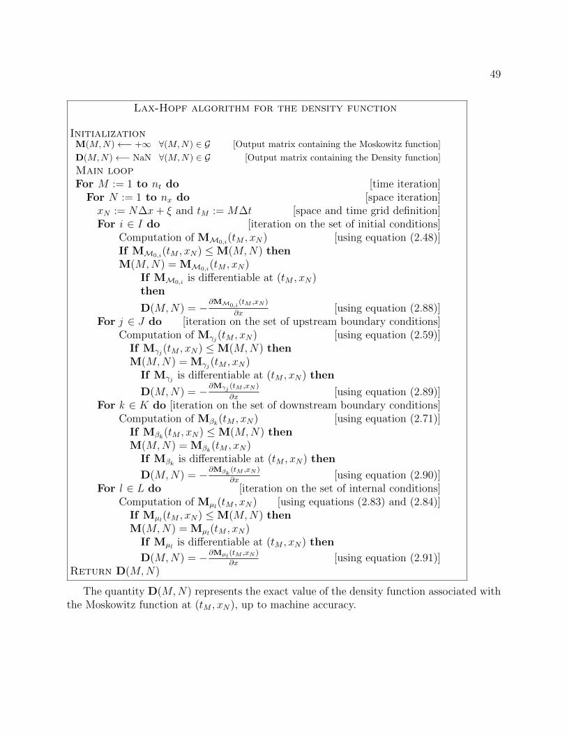
49

Lax-Hopf algorithm for the density function

InitializationM(M,N)←− +∞ ∀(M,N) ∈ G [Output matrix containing the Moskowitz function]

D(M,N)←− NaN ∀(M,N) ∈ G [Output matrix containing the Density function]

Main loopFor M := 1 to nt do [time iteration]

For N := 1 to nx do [space iteration]xN := N∆x+ ξ and tM := M∆t [space and time grid definition]For i ∈ I do [iteration on the set of initial conditions]

Computation of MM0,i(tM , xN) [using equation (2.48)]

If MM0,i(tM , xN) ≤M(M,N) then

M(M,N) = MM0,i(tM , xN)

If MM0,iis differentiable at (tM , xN)

then

D(M,N) = −∂MM0,i(tM ,xN )

∂x[using equation (2.88)]

For j ∈ J do [iteration on the set of upstream boundary conditions]Computation of Mγj(tM , xN) [using equation (2.59)]

If Mγj(tM , xN) ≤M(M,N) thenM(M,N) = Mγj(tM , xN)

If Mγj is differentiable at (tM , xN) then

D(M,N) = −∂Mγj (tM ,xN )


For k ∈ K do [iteration on the set of downstream boundary conditions]Computation of Mβk(tM , xN) [using equation (2.71)]

If Mβk(tM , xN) ≤M(M,N) thenM(M,N) = Mβk(tM , xN)

If Mβk is differentiable at (tM , xN) then

D(M,N) = −∂Mβk(tM ,xN )


For l ∈ L do [iteration on the set of internal conditions]Computation of Mµl(tM , xN) [using equations (2.83) and (2.84)]

If Mµl(tM , xN) ≤M(M,N) thenM(M,N) = Mµl(tM , xN)

If Mµl is differentiable at (tM , xN) then

D(M,N) = −∂Mµl(tM ,xN )


Return D(M,N)

The quantity D(M,N) represents the exact value of the density function associated withthe Moskowitz function at (tM , xN), up to machine accuracy.

50

2.8 Numerical examples

2.8.1 Integration of internal conditions into Hamilton-Jacobi equa-tions

In this implementation, we consider a triangular Hamiltonian as defined in example 2,with parameters ν[ = 1, γ = 1, ω = 6, ν] = 1

5and δ = ϕ∗(0) = 1. We also consider

piecewise affine initial, upstream, downstream and internal condition functions defined byequation (2.94):

M0(t, x) =

aix+ bi if t = 0,and ∃i ∈ I such that x ∈ [αi, αi+1]

+∞ otherwise

γ(t, x) =

cjt+ dj if x = ξ

and ∃j ∈ J such that t ∈ [γj , γj+1]+∞ otherwise

β(t, x) =

ekt+ fk if x = χ

and ∃k ∈ K such that t ∈ [βk, βk+1]+∞ otherwise

µp(t, x) =

gpl(t− δpl) + hpl if ∃l ∈ Lp such that

x = vpl(t− δpl) + xpland t ∈ [δpl, δpl+1]

+∞ otherwise

(2.94)

In this numerical application, we choose the following set of coefficients ai, bi, αi, cj, dj,γj, ek, fk, βk:

a := (−1,−7/2,−1/10,−7/5)b := (0,−25

2,−43

2, 92)

α := (0, 5, 10, 20, 25)c := (1, 1/2, 4/5, 7/10)d := (0, 3

2,−9

5,− 3

10)

γ := (0, 3, 11, 15, 20)e := (0, 2/5, 0, 4/5)f := (−61

2,−289

10,−221

10,−365

10)

β := (0, 4, 17, 18, 20)

(2.95)

We first compute the solution to equation (2.5) associated with (2.95) numerically usingthe Lax-Hopf algorithm. The results are shown in Figure 2.13.

51

Figure 2.13: Example of integration of an internal condition into the solution ofthe HJ PDE (2.5).Left: Computation of the solution to the mixed initial-boundary conditions problem with pa-rameters listed in (2.95). Right: Computation of the solution to the mixed initial-boundary-internal conditions problem (2.95) and (2.96). The initial, boundary and internal conditionsare represented by solid lines.

We then incorporate a single internal condition, defined by the following coefficients.v1 := (2/5, 0, 1/2, 1/2)g1 := (1/5, 1, 1/4, 0)h1 := (−18,−19,−20,−21,−21)

δ1 := (3, 8, 9, 14, 15)

(2.96)

As can be seen in Figure 2.13, the incorporation of the internal condition modifies thevalue of the solution around it and enables us to add new information.

2.8.2 Numerical validation of the Lax-Hopf algorithm (densityfunction)

We compare the Lax-Hopf algorithm and the Godunov scheme [91, 54, 48] (and its specificinstantiation as the Daganzo cell transmission model [39, 40]), which is widely used by thetransportation research community.

In this implementation, we consider a (non piecewise affine) Greenshields Hamiltoniandefined as in example 1, where ν = 1 and ρ∗ = 4 (dummy values). We consider the followinginitial and upstream boundary condition functions:

a := (−2,−4,−1)b := (0, 20,−40)α := (0, 10, 20, 30)

c := (2)d := (0)γ := (0, 20)

(2.97)

52

These initial and upstream boundary conditions were used previously in the article [91].We compute the Moskowitz and density functions solution to the initial and upstream

boundary conditions problem (2.97) using the Lax-Hopf algorithm and compare the resultswith the analytical formula derived in [91]. The results are illustrated in Figure 2.14.

Figure 2.14: Comparison between the Lax-Hopf algorithm and the analytical so-lution of problem (2.97).The solutions at times t = 0, t = 5, t = 10 and t = 15 are represented in the upper left,upper right, lower left and lower right subfigures respectively. In each of these subfigures, theanalytical solution is represented by a dashed line and the solution yielded by the Lax-Hopfalgorithm is represented using dots. The difference between the two solutions is of the orderof machine error and thus not visible on these figures.

As can be seen in Figure 2.14, the numerical solution of the LWR PDE using the Lax-Hopfalgorithm is identical to the analytical solution computed by the method of characteristicsin [16]. In addition to its high accuracy, the Lax-Hopf algorithm is not limited by the CourantFriedrichs Lewy (CFL) time step size condition inherent to many finite difference schemesand can thus compute the solution at a given time faster than finite difference schemes, suchas the Godunov scheme.

The Godunov scheme is only stable when the CFL condition ν∆t ≤ ∆x is satisfied,where ∆t and ∆x represent the discretized time and space steps. We consider the mixedinitial-boundary-internal conditions problem (2.97) as previously and compute the solutionat time t = 15 using the Godunov scheme and the Lax-Hopf algorithm, for different space

53

resolutions ∆x. The computational times are shown in Figure 2.15. For fairness of thecomparison, all algorithms presented here have been implemented in the same programminglanguage (Matlab) and run on the same platform (Thinkpad T61 running Windows XP).

Figure 2.15: Computational time comparison between the Lax-Hopf algorithmand the Godunov scheme (2.97).This figure represents the time required to compute the solution of problem (2.97) at timet = 15, using both the Godunov scheme (dots) and the Lax-Hopf algorithm (dashed line).

Figure 2.15 shows that the Lax-Hopf algorithm is significantly faster than the Godunovscheme when high accuracy is required. Indeed, the Lax-Hopf algorithm can compute thesolution at time t = 15 using only the knowledge of the initial and boundary conditions. Incontrast, the Godunov scheme has to compute the solution for each time step ∆t, which isupper-constrained by the CFL condition and thus cannot be arbitrary large.

2.8.3 Comparison with standard numerical schemes

The striking difference in terms of computational cost between the Lax-Hopf algorithmand any finite difference scheme, such as the Lax-Friedrichs scheme, is that one does notneed intermediate computations for times M ∈ {1, . . . , nt} to compute the solution at timestep nt. In other words, no iteration is needed to compute the value of the solution at anygiven time.

Another difference is that the computational cost of the Lax-Hopf algorithm is relatedto the number of piecewise affine elements in the initial, boundary and internal conditionsonly. In particular, the computational time required to solve a given problem depends

54

upon its complexity (i.e. the total number of piecewise affine elements in the definition ofthe piecewise affine initial, boundary and internal conditions). In finite difference schemeshowever, the computational time is independent of the complexity of the problem to solve.

Unlike finite difference schemes, the solution computed using the Lax-Hopf algorithm is(up to machine accuracy) exact. Indeed, the formulae (2.48), (2.59), (2.71), (2.83) and (2.84)are closed form and the minimization process used in the Lax-Hopf algorithm yields exactresults.

Note that other computational methods such as front tracking methods [19, 38, 61]can also be used to explicitly compute solutions to conservation laws, from which the HJPDE (2.5) is derived. However, the Lax-Hopf algorithm is different, since it can be ap-plied to a general concave Hamiltonian, is not event-based and does not require the explicitcomputation of shockwaves propagation.

55

Chapter 3

Convex formulations of the modelconstraints in Hamilton-Jacobi partialdifferential equations

3.1 Model constraints for well-posedness

In this section, we investigate the constraints that must apply on a general set of valueconditions to ensure that the solution to the HJ PDE satisfies all prescribed value conditions.One of the specificities of the HJ PDE (2.5) investigated in this dissertation is the fact thatthe solution itself may not reflect the value conditions that are imposed on it. Indeed,an arbitrary set of value conditions is said to apply in the strong sense if the solution isidentical to the set of value conditions (on their respective domains of definition) and inthe weak sense if at least one of the value conditions does not apply everywhere. In thefollowing, we determine the conditions on the value conditions and on the Hamiltonian ψ(·)that ensure that all value conditions apply in the strong sense.

For this, we first have to define an binary relation that characterizes the order betweengeneral concave or convex functions.

Definition 26. [Hypographical and epigraphical characterizations of pointwiseinequality between functions] Let Hyp(·) denote the hypograph of a function and Epi(·)its epigraph. Let two concave functions ψ1(·) and ψ2(·) be given. The binary relation ofinequality between these functions is defined by:

ψ1(·) ≤ ψ2(·)⇐⇒ Hyp(ψ1) ⊂ Hyp(ψ2)⇐⇒{

Dom(ψ1) ⊂ Dom(ψ2) and∀p ∈ Dom(ψ1), ψ1(p) ≤ ψ2(p)

(3.1)

Let two convex functions ϕ1(·) and ϕ2(·) be given. The binary relation of inequality

56

between these functions is defined by:

ϕ1(·) ≤ ϕ2(·)⇐⇒ Epi(ϕ1) ⊃ Epi(ϕ2)⇐⇒{

Dom(ϕ1) ⊃ Dom(ϕ2) and∀u ∈ Dom(ϕ2), ϕ1(u) ≤ ϕ2(u)

(3.2)

We now define the concept of true state, i.e. the actual value of the Moskowitz function,which plays a particular role in our estimation problem.

Definition 27. [True state] The true state M(·, ·) represents the state of the system,which could be obtained if measured by errorless sensors covering the entire space-timedomain [0, tmax]×X.

Some experimental data sets such as the NGSIM data [102] enable us to derive the truestate function M(·, ·). An example of true state function M(·, ·) derived from the NGSIMdata is illustrated in Figure 3.1.

Figure 3.1: NGSIM experimental data.This figure represents of the experimental Moskowitz surface obtained from the NGSIM data.

In most real time applications, M(·, ·) is not known, since measuring it requires a sensorobserving the state of traffic on the whole spatial domain and for all times. In the NGSIMdataset [102] for instance, the true state M(·, ·) was observed by using a camera filminga highway section from above. This data however required post-processing and was notavailable in real time.

Our data assimilation framework requires the following assumption on the true statefunction M(·, ·).

57

Fact 1. [Mathematical properties of the state] The true state M(·, ·) is assumed to beLipschitz-continuous [41, 42].

Note that the Lipschitz continuity of M(·, ·) implies the existence almost everywhere and

boundedness of the flow ∂M(t,x)∂t

and the density −∂M(t,x)∂x

. This assumption is true for mostphysical systems, including highway traffic modeling [41]. Note also that no assumptionis made that M(·, ·) satisfies the HJ PDE (2.5) exactly, which is in general true for mostphysical systems (i.e. their state does not satisfy a model perfectly).

The true state function enables the definition of corresponding true value conditions,which will be later shown to satisfy specific constraints.

Definition 28. [True value condition] Let M(·, ·) denote the true state of the system.A true value condition c(·, ·) is a function defined on a subset of [0, tmax]×X and satisfying:

c(t, x) :=

{M(t, x) if(t, x) ∈ Dom(c)+∞ otherwise

(3.3)

The following property holds:

Proposition 22. [Minimum of true value conditions] Let cj(·, ·)j∈J be a finite familyof true value conditions, as in definition 28. The minimum c(·, ·) := min

j∈J(cj(·, ·)) of the true

value conditions cj(·, ·) is also a true value condition, whose domain of definition is given by:

Dom(c) :=⋃j∈J

Dom(cj) (3.4)

In addition, we have the following property:

∀j ∈ J, ∀(t, x) ∈ Dom(cj), c(t, x) = cj(t, x) (3.5)

Proof — The proof of this proposition is straightforward and follows directly fromdefinition 28. �

A value condition represents some knowledge of the true state of the system, which isused in conjunction with the HJ PDE (2.5) to construct an estimated state of the system.

Definition 29. [Estimated state] Let a value condition c(·, ·) be defined as in defini-tion 2. The estimated state is defined as the solution (2.20) associated with c(·, ·) and theHamiltonian ψ(·) and denoted by Mc,ψ(·, ·).

Note the ψ(·) index in the definition above, which as previously indicates that the value ofthe solution Mc,ψ(·, ·) associated with the value condition c(·, ·) depends (implicitly) on theHamiltonian of the HJ PDE. As a consequence of theorem 1, the estimated state Mc,ψ(·, ·)is a solution to (2.5) in the B-J/F sense. However, the estimated state does not necessarilysatisfy the true value condition that we want to impose on it [31, 32].

58

In the following section, we find the conditions on a finite set of value conditions (cj(·, ·))j∈Jsuch that all of these value conditions apply in the strong sense when solving (2.5). In thiscase, we say that the value conditions are compatible with the model. The correspondingconstraints on the value conditions are called model compatibility constraints. The valueconditions (cj(·, ·))j∈J satisfy the model compatibility constraints if and only if the followingequality is true:

∀j ∈ J, ∀(t, x) ∈ Dom(cj), Mcj ,ψ(t, x) = cj(t, x) (3.6)

The following section presents an equivalent formulation of (3.6), based on the propertiesof the solution (2.20), which results in algebraic conditions to be verified for (3.6) to besatisfied.

3.1.1 Compatibility conditions

Because of the inf-morphism property (2.36) and the Lax-Hopf formula (2.20), the equal-ity (3.6) can be decomposed as a set of inequalities known as compatibility conditions, whichwe now express.

Proposition 23. [Compatibility conditions] Let us define a finite family of value condi-tion functions cj(·, ·), j ∈ J as in definition 2 and their minimum c(·, ·) := min

j∈Jcj(·, ·). The

estimated state Mc,ψ(·, ·) associated with c(·, ·) satisfies the property (3.6) if and only if thefollowing set of inequalities is satisfied:

Mci,ψ(t, x) ≥ cj(t, x), ∀(t, x) ∈ Dom(cj), ∀i ∈ J, ∀j ∈ J (3.7)

Proof — Let us first start from (3.6). By definition of c(·, ·), we have that (t, x) ∈Dom(c) if and only if (t, x) ∈ Dom(cj) for some j ∈ J . Hence, using equation (3.5), we canequivalently rewrite (3.6) as:

∀j ∈ J, ∀(t, x) ∈ Dom(cj), Mc,ψ(t, x) = cj(t, x) (3.8)

We now prove that (3.8) implies (3.7). The inf-morphism property (2.36) implies thatthe estimated state Mc,ψ(·, ·) associated with the value condition c(·, ·) is the minimum ofthe estimated states Mci,ψ(·, ·) associated with the value conditions ci(·, ·):

Mc,ψ(t, x) = mini∈J

Mci,ψ(t, x) (3.9)

Hence, the condition (3.8) implies the constraints (3.7).Reciprocally, we prove that (3.7) implies the equality (3.8). When (3.7) is satisfied,

equation (3.9) implies that Mc,ψ(t, x) ≥ cj(t, x) for all j ∈ J and for all (t, x) ∈ Dom(cj).The converse inequality is obtained from the Lax-Hopf formula (2.20):

59

Mcj ,ψ(t, x) = inf(u,T )∈Dom(ϕ∗)×R+

(cj(t− T, x+ Tu) + Tϕ∗(u)) (3.10)

By taking T = 0 and u ∈ Dom(ϕ∗) in (3.10), we have that ∀j ∈ J, ∀(t, x) ∈Dom(cj), Mcj ,ψ(t, x) ≤ cj(t, x). By the inf-morphism property, this last inequality im-plies ∀j ∈ J, ∀(t, x) ∈ Dom(cj), Mc,ψ(t, x) ≤ cj(t, x) which completes the proof. �

We assumed in this section that ψ(·) was given. In the next section, we define conditionson ψ(·) and the true state M(·, ·) which ensure that the compatibility conditions (3.7) asso-ciated with true value condition cj(·, ·) are automatically satisfied, i.e. the equality (3.6) issatisfied. In general, the true state M(·, ·) not given, but some of its properties are known.Thus, the following results amount to finding the proper Hamiltonian ψ(·) such that thecompatibility conditions (3.7) are satisfied.

3.1.2 Sufficient conditions on the Hamiltonian for compatibilityof true value conditions

While the true state is generally unknown, the properties of its derivatives have beenextensively studied in the literature [56, 72, 86]. Note that by (2.4), the derivatives of thetrue state function represent the true density and true flow functions. We assume that wecan measure some values of the derivatives of M(·, ·) which are representative of the rangeof physical measurements of the system. Using these measurements, we define a particularclass of Hamiltonians as follows.

Proposition 24. [Upper estimate of the Hamiltonian]. For a given true state M(·, ·),we define the set B(M) as follows:

B(M) :={(−∂M(t,x)

∂x , ∂M(t,x)∂t

), (t, x) ∈ [0, tmax]×X such that M(·, ·) is differentiable

}There exists a concave and upper semicontinuous function ψ0(·) such that:

B(M) ⊂ Hyp(ψ0) (3.11)

Proof — Recall that the true state is Lipschitz-continuous by assumption. Thus, itsderivatives are defined almost everywhere and bounded, which implies the boundedness ofB(M). Hence, we can choose for ψ0(·) any concave function greater than the upper concaveenvelope of B(M). �

Note that the choice of a function ψ0(·) compatible with (3.11) is not unique. An exampleof choice of ψ0(·) satisfying (3.11) is illustrated in Figure 3.2 later.

The conditions (3.7) are necessarily satisfied for a true value condition c(·, ·) and for aHamiltonian ψ0(·) satisfying (3.11), as shown in the following proposition.

60

Proposition 25. [Compatibility property for true value conditions] Let us define afinite set of true value condition functions cj(·, ·), j ∈ J as in definition 28, a concave andupper semicontinuous Hamiltonian ψ0(·) satisfying (3.11) and its associated convex transformϕ∗0 as in (2.7). Let us also define the set of solutions Mcj ,ψ0(·, ·) associated with cj(·, ·) asin (2.20). Given these assumptions, the set of inequalities (3.7) are satisfied.

Proof — In the present case, the compatibility conditions (3.7) can be written as:

Mci,ψ0(t, x) ≥ cj(t, x), ∀(t, x) ∈ Dom(cj), ∀i ∈ J, ∀j ∈ J (3.12)

Let us fix i ∈ J , j ∈ J and (t, x) ∈ Dom(cj).We first express Mci,ψ0(t, x) in terms of ci(·, ·) using the Lax-Hopf formula (2.20):

Mci,ψ0(t, x) = inf(u,T )∈Dom(ϕ∗0)×R+

(ci(t− T, x+ Tu) + Tϕ∗0(u)) (3.13)

Since (t, x) ∈ Dom(cj), we have by definition 28 that cj(t, x) = M(t, x). Hence, we canwrite the inequality (3.12) which we want to prove as:

inf(T,u)∈[0,tmax]×Dom(ϕ∗

0)(ci(t− T, x+ Tu) + Tϕ∗0(u)) ≥M(t, x) (3.14)

By definition 28, we have that ci(t − T, x + Tu) ≥ M(t − T, x + Tu) for all (T, u) ∈[0, tmax]×Dom(ϕ∗0). Indeed, ci(t−T, x+Tu) = M(t−T, x+Tu) if (t−T, x+Tu) ∈ Dom(ci)and that ci(t− T, x+ Tu) = +∞ otherwise. Hence, if the equation (3.15) below is satisfied,then inequality (3.14) will be automatically true:

inf(T,u)∈[0,tmax]×Dom(ϕ∗

0)

(M(t− T, x+ Tu) + Tϕ∗0(u)

)≥M(t, x) (3.15)

We now prove that (3.15) holds. Since M(·, ·) is Lipschitz-continuous by assumption andassuming that M(·, ·) is differentiable almost everywhere on {(t− τ, x+ τu), τ ∈ [0, T ]}, wecan write:

M(t− T, x+ Tu) + Tϕ∗0(u)−M(t, x) =∫ T0

(−∂M(t−τ,x+τu)

∂t + u∂M(t−τ,x+τu)∂x + ϕ∗0(u)

)dτ (3.16)

Since ψ0(·) is concave and upper semicontinuous, it is equal to its Legendre-Fenchelbiconjugate [8]. Hence, we have that ψ0(ρ) = inf

u∈Dom(ϕ∗0)(−ρu+ ϕ∗0(u)) and thus that ψ0(ρ) ≤

−ρu + ϕ∗0(u) for all u ∈ Dom(ϕ∗0). This result enables us to derive the following inequalityfrom equation (3.16):

M(t− T, x+ Tu) + Tϕ∗0(u)−M(t, x) ≥∫ T0

(− ∂M(t−τ,x+τu)

∂t + ψ0


∂x

))dτ (3.17)

61

Using (3.11), we have that −∂M(t−τ,x+τu)∂t

+ψ0


∂x

)≥ 0 for all (τ, u) ∈ [0, T ]×

Dom(ϕ∗0). Since T > 0, the right hand side of equation (3.17) is nonnegative, which impliesthe following inequality:

∀(T, u) ∈ R+ ×Dom(ϕ∗0), M(t− T, x+ Tu) + Tϕ∗0(u)−M(t, x) ≥ 0 (3.18)

Equation (3.15) is obtained from equation (3.18) by taking the infimum over (T, u) ∈R+ × Dom(ϕ∗0), which completes the proof. Note that if M(·, ·) is not differentiable al-most everywhere on the set {(t− τ, x+ τu), τ ∈ [0, T ]}, it will be differentiable on the set{(t− τ, x+ δx+ τu), τ ∈ [0, T ]} for a small δx, by Lipschitz-continuity. Hence, we havethat M(t− T, x+ δx+ Tu) + Tϕ∗0(u)−M(t, x+ δx) ≥ 0, which implies M(t− T, x+ δx+Tu) + Tϕ∗0(u)−M(t, x+ δx) ≥ 0 by (Lipschitz) continuity of M(·, ·). �

Proposition 25 thus implies that the estimated state Mc,ψ0(·, ·) associated with any truevalue condition c(·, ·) satisfies the imposed true value condition when the Hamiltonian ψ0(·)satisfies (3.11).

Because of the order-preserving property of (2.7), the constraints (3.7) are satisfied fora given Hamiltonian ψ1(·) only if they are also satisfied for any Hamiltonian ψ2(·) greaterthan ψ1(·), as expressed by the following proposition.

Proposition 26. [Hamiltonian inequality property] Let us define a finite set of truevalue conditions cj(·, ·), j ∈ J as in definition 28. Let us also define two concave andupper semicontinuous Hamiltonians ψ1(·) and ψ2(·), satisfying ψ1(·) ≤ ψ2(·). The associatedsolutions Mcj ,ψ1(·, ·) and Mcj ,ψ2(·, ·) associated with the true value condition cj(·, ·) aredefined by (2.20). We have the following property:


implies


Proof — The proof of this proposition is a direct consequence of the following property:

Mci,ψ1(t, x) ≤Mci,ψ2(t, x), ∀(t, x) ∈ [0, tmax]×X, ∀i ∈ J (3.21)

Indeed, since ψ1(·) ≤ ψ2(·), we have that pu + ψ1(p) ≤ pu + ψ2(p) ∀(p, u) ∈ R2. Hence,the convex transforms ϕ∗1(·) and ϕ∗2(·) respectively associated with ψ1(·) and ψ2(·) satisfyϕ∗1(·) ≤ ϕ∗2(·).

Let us fix (t, x, j) ∈ [0, tmax]×X × J . The solutions Mci,ψ1(t, x) and Mci,ψ2(t, x) can beexpressed using the following Lax-Hopf formulae:

62


(ci(t− T, x+ Tu) + Tϕ∗1(u))


(ci(t− T, x+ Tu) + Tϕ∗2(u))(3.22)

Since ϕ∗1(·) ≤ ϕ∗2(·), we have that Dom(ϕ∗2) ⊂ Dom(ϕ∗1). Hence, equation (3.22) im-plies (3.21) and thus, (3.19) implies (3.20). �

In consequence, the smallest concave function satisfying (3.11), illustrated in Figure 3.2plays a particular role in our problem.

Figure 3.2: Illustration of an upper estimate function ψ0(·).In this figure, the horizontal axis represents the density and the vertical axis the flow. Thescatter plot represents the values of flow and density obtained from experimental traffic flow

data [103]. Each point in this plot is a given(−∂M(t,x)

∂x, ∂M(t,x)

∂t

)for some (t, x) ∈ [0, tmax]×X.

A typical example of upper estimate function ψ0(·) is the upper concave envelope of thepoints, represented by a dashed line and which satisfies (3.11).

Proposition 27. [Smallest concave upper estimate] Let M be given and let B(M) bedefined as in proposition 24. Let C be the set of upper semicontinuous concave functionsfrom R to R and let us define the set of functions A by:

A :={ψ ∈ C such that B(M) ⊂ Hyp(ψ)

}(3.23)

Let us define the function ψinf(·) as:

Hyp(ψinf) :=⋂ψ∈A

Hyp(ψ) (3.24)

63

The function ψinf(·) defined by (3.24) is the smallest element of A.

Proof — The set A is not empty by proposition 24 and thus the function ψinf(·) definedby (3.24) exists. We now prove that ψinf(·) is the smallest element of A. Let ψ(·) ∈ A. Sinceψ(·) is concave, upper semicontinuous and satisfies (3.11), its hypograph is closed, convexand contains the set B(M). By (3.24), the hypograph of ψinf(·) is thus closed, convex andcontains B(M) since it is the (infinite) intersection of closed and convex sets containingB(M). Hence, ψinf is concave, upper semicontinuous and satisfies (3.11), which impliesψinf ∈ A. The function ψinf(·) is also the smallest element of A, since any element ψ(·) of Asatisfies Hyp(ψinf(·)) ⊂ Hyp(ψ(·)) by (3.24). �

Proposition 28. [Minimal conditions] Let A be defined as in proposition 27 and letψinf(·) be defined as in as in (3.24). Let ψ(·) ∈ A and let us define a finite set of truevalue conditions cj(·, ·), j ∈ J and their associated solutions Mcj ,ψinf

(·, ·) and Mcj ,ψ(·, ·) asin (2.20). Given the above definitions, we have the following property:

Mci,ψ(t, x) ≥ cj(t, x), ∀(t, x) ∈ Dom(cj), ∀i ∈ J, ∀j ∈ J, ∀ψ(·) ∈ A (3.25)

if and only if

Mci,ψinf(t, x) ≥ cj(t, x), ∀(t, x) ∈ Dom(cj), ∀i ∈ J, ∀j ∈ J (3.26)

Proof — The conditions (3.25) imply (3.26), since ψinf(·) ∈ A by proposition 27.Conversely, the conditions (3.26) imply (3.25), by proposition 26, remarking thatHyp(ψinf) ⊂Hyp(ψ). �

Proposition 28 enables the verification of the conditions (3.25) for a true value condi-tion c(·, ·) and for all Hamiltonians ψ(·) satisfying (3.11) using the conditions (3.26) only.

We now present some important properties of the model compatibility constraints.

3.2 Properties of the model compatibility constraints

3.2.1 Concavity property of the solutions with respect to theircoefficients

Because of the Lax-Hopf formula (2.20), the solutions associated with affine initial,boundary and internal conditions have a concavity property with respect to some of theircoefficients, which we now present.

Proposition 29. [Concavity property of the solution associated with an affineinitial condition] The solution MM0,i

(·, ·) associated with the affine initial condition (2.39)is a concave function of the coefficients ai and bi.

64

Proof — The Lax-Hopf formula (2.20) associated with the solution MM0,i(·, ·) can be

written as:

MM0,i(t, x) = inf

u∈Dom(ϕ∗) s. t. (x+tu)∈[αi,βi](ai(x+ tu) + bi + tϕ∗(u)) (3.27)

Let us fix (t, x, u) ∈ [0, tmax] ×X × Dom(ϕ∗). The function f(·, ·) defined as f(ai, bi) =ai(x + tu) + bi + tϕ∗(u) is concave (indeed, affine). Hence, the solution MM0,i

(t, x) is aconcave function of (ai, bi), since it is the infimum of concave functions of (ai, bi) [18, 87].�

Proposition 30. [Concavity property of the solution associated with an affineupstream boundary condition] The solution Mγj(·, ·) associated with the affine upstreamboundary condition (2.49) is a concave function of the coefficients cj and dj.

Proof — The Lax-Hopf formula (2.20) associated with the solution Mγj(·, ·) can bewritten as:

Mγj(t, x) = infT∈[− ξ−x

ν[,+∞


(cj(t− T ) + dj + Tϕ∗

(ξ − xT

))(3.28)

Let us fix (t, x, T ) ∈ [0, tmax]×X ×[− ξ−x

ν[,+∞

[∩[t− γj+1, t− γj

]. The function g(·, ·)

defined as f(cj, dj) = cj(t − T ) + dj + Tϕ∗(ξ−xT

)is concave (indeed, affine). Hence, the

solution Mγj(t, x) is a concave function of (cj, dj), since it is the infimum of concave functionsof (cj, dj) [18, 87]. �

Proposition 31. [Concavity property of the solution associated with an affinedownstream boundary condition] The solution Mβk(·, ·) associated with the affine down-stream boundary condition (2.61) is a concave function of the coefficients ek and fk.

Proof — The Lax-Hopf formula (2.20) associated with the solution Mβk(·, ·) can bewritten as:


ν],+∞[∩[t−βk+1,t−βk]

(ek(t− T ) + fk + Tϕ∗

(χ− xT

))(3.29)

Let us fix (t, x, T ) ∈ [0, tmax] ×X ×[χ−xν],+∞

[∩[t− βk+1, t− βk

]. The function h(·, ·)

defined as f(ek, fk) = ek(t − T ) + fk + Tϕ∗(χ−xT

)is concave (indeed, affine). Hence, the

solution Mβk(t, x) is a concave function of (ek, fk), since it is the infimum of concave functionsof (ek, fk) [18, 87]. �

65

Proposition 32. [Concavity property of the solution associated with an affineinternal condition] The solution Mµl(·, ·) associated with the internal condition (2.73) isa concave function of the coefficients gl and hl.

Proof — The Lax-Hopf formula (2.20) associated with the solution Mµl(·, ·) can bewritten [31, 32] as:

Mµl(t, x) = infT∈R+∩[t−δl,t−γl]

gl(t− T − γl) + hl + Tϕ∗(xl + vl(t− γl − T )− x

T

)(3.30)

Let us fix (t, x, T ) ∈ [0, tmax] × X × R+. The function d(·, ·) defined as d(gl, hl) :=

gl(t − T − γl) + hl + Tϕ∗(xl+vl(t−γl−T )−x

T

)is concave (indeed, affine). Hence, the solution

Mµl(t, x) is a concave function of (gl, hl), since it is the infimum of concave functions [18, 87].�

3.2.2 Convex formulation of the model compatibility constraints

For the initial, boundary and internal conditions defined by (2.39), (2.49), (2.61) and (2.73),the model compatibility constraints (3.7) define constraints on the coefficients ai, bi, cj, dj,ek, fk, gl, hl. We now prove that these constraints are convex.

Proposition 33. [Convexity property of the model constraints] Let initial, boundaryand internal conditions be defined as in (2.39), (2.49), (2.61) and (2.73), for i ∈ I, j ∈ J , k ∈K and l ∈ L where I, J , K and L are finite sets. The model compatibility constraints (3.7)are convex inequalities in the coefficients ai, bi, cj, dj, ek, fk, gl and hl.

Proof — The constraints (3.7) are of the form:

Mcn(t, x) ≥ cm(t, x), ∀(t, x) ∈ Dom(cm), ∀n ∈ N, ∀m ∈ N (3.31)

Let (n,m) ∈ N2 and (t, x) ∈ Dom(cm). The quantity cm(t, x) is an affine function ofthe coefficients ai, bi, cj, dj, ek, fk, gl and hl. In addition, Mcn(t, x) is a concave functionof ai, bi, cj, dj, ek, fk, gl and hl. The constraint Mcn(t, x) ≥ cm(t, x) can be written as−Mcn(t, x) + cm(t, x) ≤ 0 where −Mcn(t, x) + cm(t, x) is a convex function (as the sum ofconvex functions) of ai, bi, cj, dj, ek, fk, gl and hl. Hence, Mcn(t, x) ≥ cm(t, x) is a convexconstraint [18] in ai, bi, cj, dj, ek, fk, gl and hl. �

Proposition 33 states that the inequality constraints (3.7) define a convex set in the space(ai, bi, cj, dj, ek, fk, gl, hl). Using this property, we pose inverse modeling problems as convexoptimization programs in chapter 4.

66

3.2.3 Monotonicity property of the model compatibility condi-tions

An important property of the model compatibility constraints (3.7) is their monotonicitywith respect to new data, outlined in the following proposition.

Proposition 34. [Monotonicity property] Let a set of affine initial, boundary and in-ternal conditions be defined as in (2.39), (2.49), (2.61) and (2.73) for i ∈ I, j ∈ J , k ∈ Kand l ∈ L where I, J , K and L are finite sets. The convex set defined by the inequalityconstraints (3.31) is decreasing (in the sense of inclusion) as new initial, boundary or internalconditions are added.

Proof — The model compatibility constraints can be written as:

Mcn(t, x) ≥ cm(t, x), ∀(t, x) ∈ Dom(cm), ∀n ∈ N, ∀m ∈ N (3.32)

Let N ⊂ R|N | be the convex set defined by (3.32). We now add a finite number of newvalue conditions cp, defined for p ∈ P . The model compatibility constraints become:

Mcn(t, x) ≥ cm(t, x), ∀(t, x) ∈ Dom(cm), ∀n ∈ N ∪ P, ∀m ∈ N ∪ P (3.33)

Let M ⊂ R|N |+|P | be the convex set defined by (3.33). Since the constraints (3.33) im-ply (3.32), we the projection of M on R|N | is a subset of N , which completes the proof.�

The above property is very important in practice, since it ensures that the feasible setsdecreases in size when new data is added. Hence, the results of the estimation problemsderived in the next chapter necessarily improve when new data is added, which is not thecase for Monte-Carlo based estimation methods.

67

Chapter 4

Applications

In chapter 3, we established the convexity of the model compatibility constraints. We nowuse this result to solve different estimation problems arising in traffic-flow engineering. Forthis, we first derive the relationship between value condition coefficients and measurementdata. We then instantiate the convex model compatibility constraints as linear inequalitiesfor triangular Hamiltonians defined by example 2. Similarly, we show that the measurementdata yields data compatibility constraints, which can also be formulated as linear inequalities.

4.1 Traffic flow measurement data and value conditions

In the context of traffic flow monitoring, measurement data traditionally originates fromEulerian (i.e. fixed) sensors. This is in contrast with new Lagrangian (i.e. mobile) sensors,which sense traffic conditions while moving alongside it.

4.1.1 Fixed detector data

Fixed sensors are currently the backbone of traffic monitoring. They measure variousquantities related to traffic flow at a fixed location and for all times. Current fixed-sensortechnology includes:

• Inductive loop detectors, such as the Performance Measurement System PeMS [103]in California and magnetometers [24] are based on measurements of the inductanceof an electromagnetic loop. They can measure two quantities: the flow of vehiclesabove the sensor and the occupancy which can be related to the density of vehiclesabove the sensor. Dual loop detector arrangements [103], as well as some classes ofmagnetometers [24] can also directly measure traffic speed.

• Speed radars, which are measuring the doppler shift as well as the time of flight ofelectromagnetic waves. They can measure three quantities: the flow and density ofvehicles around the sensor, as well as the average traffic speed.

68

• Speed cameras, which are paired with image recognition systems. They usually mea-sure flow, density and average traffic speed.

One of the biggest problems associated with the fixed sensing infrastructure is theirdeployment and maintenance costs. Since this sensing infrastructure is dedicated (i.e. theinfrastructure cannot be used to sense other physical phenomena besides traffic flow), thesehigh costs are limiting the deployment of new sensors. In practice, the Departments ofTransportation (DOTs) are operating these sensors, and usually have to spend their fundingon more urgent issues.

4.1.2 Mobile sensor data

The emergence of new portable computational platforms with communication and sens-ing capabilities, provides the engineering community with unprecedented opportunities forsensing. In the context of traffic flow, cellular phones [97, 57] located onboard vehicles andequipped with positioning systems such as the GPS can act as traffic sensors. Other pos-sible mobile sensing systems exist, including toll tag readers such as the FasTrak system inCalifornia.

All mobile sensing systems pose an additional mathematical and computational challengewith respect to fixed sensors. Since most of the current traffic sensing systems are fixed,most of the estimation techniques for traffic-flow engineering are not specifically designed toincorporate mobile measurements.

In order to estimate the state of traffic based on Eulerian and Lagrangian sensor measure-ments, we first need to establish the relation between the measurement data and the valueconditions which incorporate the measurement constraints into the HJ PDE (2.5). This willbe explained later in the thesis

4.1.3 Experimental setup

In the following sections, we pose different problems arising in transportation engineeringas Linear Programs (LPs) or series of LPs and test their performance using experimentaldata from the Mobile Century [57] experiment.

In all numerical applications, we consider a 3.858 km long spatial domain, located be-tween the PeMS [103] stations 400536 and 400284 on Highway I − 880 N in Hayward,California. The measurement data comes from two sources. The flow data qmeas

in (·) andqmeasout (·) is generated by the PeMS stations 400536 and 400284 respectively. The probe lo-

cation and timing data comes from GPS measurements generated by Nokia N95 cellphoneslocated onboard probe vehicles. The layout is illustrated in Figure 4.1.

69

Figure 4.1: Experiment site layout.The upstream and downstream PeMS stations are delimiting a 3.858 km spatial domain,outlined by a solid line. The direction of traffic flow is represented by an arrow.

The complete experimental setting is described in [57]. The data set used in all numericalapplications of this dissertation can be freely downloaded from [101].

All LPs have been implemented in Matlab, using the package CVX [55]. The problemssolved in this dissertation are relatively tractable: they typically involve thousands of vari-ables and constraints and can be solved numerically in a few seconds on a typical laptopcomputer.

4.1.4 Link between measurement data and value conditions

In our specific application, the sensor data does not provide the initial condition of theproblem, since this would require us instrumenting the entire spatial domain. Fixed traf-fic sensors traditionally measure the inflow and outflow of vehicles on the spatial domain,which are related to the upstream and downstream boundary conditions. In addition tofixed sensors, mobile sensors onboard vehicles track the vehicle trajectory and thus gener-ate internal conditions [31]. The formal link between traffic measurement data and valuecondition (boundary and internal conditions) blocks is shown in the following definition.

Definition 30. [Affine upstream, downstream and internal conditions] Let us defineN = {0, . . . , nmax} and M = {0, . . . ,mmax}. For all n ∈ N and m ∈M, we define the following

70

upstream, downstream and internal conditions:

γn(t, x) =

∑n−1

i=0 qin(i)T + qin(n)(t− nT ) if x = ξand t ∈ [nT, (n+ 1)T ]

+∞ otherwise(4.1)

βn(t, x) =

{∑n−1i=0 qout(i)T + qout(n)(t− nT )−∆ if x = χ and t ∈ [nT, (n+ 1)T ]

+∞ otherwise(4.2)

µm(t, x) =

Lm + rm(t− tmin(m)) if x = xmin(m) + vmeas(m)(t− tmin(m))

and t ∈ [tmin(m), tmax(m)]+∞ otherwise

(4.3)

where vmeas(m) = xmax(m)−xmin(m)tmax(m)−tmin(m)

.

The domains of definitions of these functions are illustrated in Figure 4.2.

Figure 4.2: Illustration of the domains of the possible value conditions used toconstruct the solution of the Moskowitz HJ PDE.The time is represented by the horizontal axis, while the location is represented by thevertical axis. The coefficients ξ and χ represent respectively the upstream and downstreamboundaries of the highway segment of interest.

The coefficients in equations (4.1), (4.2) and (4.3) can be physically interpreted as follows:

71

qin(n) average inflow between times nT and (n+1)Tqout(n) average outflow between times nT and (n+1)T∆ initial number of vehicles on the highway section

tmin(m) initial time at which the internal condition m appliestmax(m) final time at which the internal condition m appliesxmin(m) initial location at which the internal condition m appliesxmax(m) final location at which the internal condition m appliesvmeas(m) speed of the internal condition mLm label of the vehicle m at time tmin(m)rm rate of change of the label of vehicle m

(4.4)

Since the Moskowitz function is increasing in time and decreasing in space, the coefficientsof (4.1), (4.2) and (4.3) satisfy the following conditions:

∆ ≥ 0 positivity of the initial number of vehicles∀n ∈ N, qin(n) ≥ 0 positivity of the inflow∀n ∈ N, qout(n) ≥ 0 positivity of the outflow∀m ∈M, rm ≥ 0 positivity of the passing rate

(4.5)

The monotonicity properties of the Moskowitz function with respect to its variables followdirectly from the positivity of flow and density functions (2.4) and are derived in [80].

Some of the above coefficients can be obtained (with some error) through traffic measure-ment data. Inductive loop detectors [103] and speed radars located in ξ and χ can measurethe inflow qin(n) and outflow qout(n) for all time intervals [nT, (n + 1)T ]. The coefficientstmin(m), tmax(m), xmin(m) and xmax(m) can be obtained using vehicle positioning systems,such as GPS-enabled cellphones onboard vehicles [101]. In contrast, the coefficients Lm andrm cannot be measured using conventional traffic sensors. Similarly, the initial number of ve-hicles ∆ cannot be measured using conventional sensors. Hence, the available measurementsdo not enable us to define the upstream (4.1), downstream (4.2) and internal conditions (4.3)univocally. In order to estimate the state M(·, ·) of the system, one has to estimate the co-efficients (4.4), which are constrained both by the model and the measurement data.

In the applications of this dissertation, the coefficients xmin(m), xmax(m), tmin(m) andtmax(m) are measured by are measured by GPS systems, which are very accurate. Hence,we assume that these coefficients are fixed. Given this assumption, we define the decisionvariable of our estimation problems as follows.

Definition 31. The coefficients of the upstream, downstream and internal conditions to beestimated are defined by the following decision variable:

y := (qin(1), . . . , qin(nmax), qout(1), . . . , qout(nmax), L1, . . . , Lmmax , r1, . . . , rmmax) (4.6)

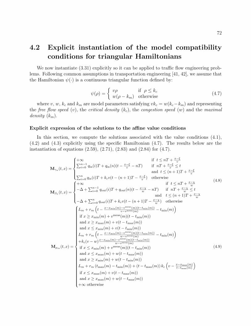
72

4.2 Explicit instantiation of the model compatibility

conditions for triangular Hamiltonians

We now instantiate (3.31) explicitly so it can be applied to traffic flow engineering prob-lems. Following common assumptions in transportation engineering [41, 42], we assume thatthe Hamiltonian ψ(·) is a continuous triangular function defined by:

ψ(ρ) =

{vρ if ρ ≤ kcw(ρ− km) otherwise

(4.7)

where v, w, kc and km are model parameters satisfying vkc = w(kc−km) and representingthe free flow speed (v), the critical density (kc), the congestion speed (w) and the maximaldensity (km).

Explicit expression of the solutions to the affine value conditions

In this section, we compute the solutions associated with the value conditions (4.1),(4.2) and (4.3) explicitly using the specific Hamiltonian (4.7). The results below are theinstantiation of equations (2.59), (2.71), (2.83) and (2.84) for (4.7).

Mγn(t, x) =

+∞ if t ≤ nT + x−ξ

v∑n−1i=0 qin(i)T + qin(n)(t− x−ξ

v − nT ) if nT + x−ξv ≤ t

and t ≤ (n+ 1)T + x−ξv∑n

i=0 qin(i)T + kcv(t− (n+ 1)T − x−ξv ) otherwise

Mβn(t, x) =

+∞ if t ≤ nT + x−χ

w

−∆ +∑n−1i=0 qout(i)T + qout(n)(t− x−χ

w − nT ) if nT + x−χw ≤ t

and t ≤ (n+ 1)T + x−χw

−∆ +∑ni=0 qout(i)T + kcv(t− (n+ 1)T − x−χ

w ) otherwise

(4.8)

Mµm(t, x) =

Lm + rm

(t− x−xmin(m)−vmeas(m)(t−tmin(m))

v−vmeas(m) − tmin(m))

if x ≥ xmin(m) + vmeas(m)(t− tmin(m))

and x ≥ xmax(m) + v(t− tmax(m))

and x ≤ xmin(m) + v(t− tmin(m))

Lm + rm

(t− x−xmin(m)−vmeas(m)(t−tmin(m))

w−vmeas(m) − tmin(m))

+kc(v − w)x−xmin(m)−vmeas(m)(t−tmin(m))w−vmeas(m)

if x ≤ xmin(m) + vmeas(m)(t− tmin(m))

and x ≤ xmax(m) + w(t− tmax(m))

and x ≥ xmin(m) + w(t− tmin(m))

Lm + rm (tmax(m)− tmin(m)) + (t− tmax(m)) kc

(v − x−xmax(m)

t−tmax(m)

)if x ≤ xmax(m) + v(t− tmax(m))

and x ≥ xmax(m) + w(t− tmax(m))

+∞ otherwise

(4.9)

73

Explicit instantiation of the model constraints

For the specific boundary and internal conditions (4.1), (4.2) and (4.3), the model com-patibility constraints (3.31) are:

Mγn(t, ξ) ≥ γp(t, ξ) ∀t ∈ [pT, (p+ 1)T ],∀(n, p) ∈ N2 (i)

Mγn(t, χ) ≥ βp(t, χ) ∀t ∈ [pT, (p+ 1)T ],∀(n, p) ∈ N2 (ii)

Mγn(t, x) ≥ µm(t, x) ∀(t, x) ∈ Dom(µm),∀n ∈ N,∀m ∈M (iii)

Mβn(t, ξ) ≥ γp(t, ξ) ∀t ∈ [pT, (p+ 1)T ],∀(n, p) ∈ N2 (iv)

Mβn(t, χ) ≥ βp(t, χ) ∀t ∈ [pT, (p+ 1)T ],∀(n, p) ∈ N2 (v)

Mβn(t, x) ≥ µm(t, x) ∀(t, x) ∈ Dom(µm),∀n ∈ N,∀m ∈M (vi)

Mµm(t, ξ) ≥ γp(t, ξ) ∀t ∈ [pT, (p+ 1)T ],∀(m, p) ∈M× N (vii)

Mµm(t, χ) ≥ βp(t, χ) ∀t ∈ [pT, (p+ 1)T ],∀(m, p) ∈M× N (viii)

Mµm(t, x) ≥ µp(t, x) ∀(t, x) ∈ Dom(µp),∀(m, p) ∈M2 (ix)

(4.10)

Although inequalities (4.10) are a function of the decision variable (4.6), they cannotnecessarily be expressed as linear inequalities (in terms of the decision variable) in general.However, because of the specific structure of the solutions (4.8) for triangular Hamiltonians,the inequalities (4.10) can be rewritten as a finite number of linear inequality constraints, asshown in the following proposition.

Proposition 35. [Model constraints for triangular Hamiltonians] For triangularHamiltonians defined by (4.7), the inequality constraints (4.10) can be expressed as a fi-nite number of inequality constraints:

Mγn(pT, ξ) ≥ γp(pT, ξ) ∀(n, p) ∈ N2 (i)

Mγn(pT, χ) ≥ βp(pT, χ) ∀(n, p) ∈ N2 (ii)(a)

Mγn(nT + χ−ξv , χ) ≥ βp(nT + χ−ξ

v , χ) ∀(n, p) ∈ N2 such that

nT + χ−ξv ∈ [pT, (p+ 1)T ] (ii)(b)

(4.11)

Mγn(tmin(m), xmin(m)) ≥ µm(tmin(m), xmin(m)) ∀n ∈ N,∀m ∈M (iii)(a)

Mγn(tmax(m), xmax(m)) ≥ µm(tmax(m), xmax(m)) ∀n ∈ N,∀m ∈M (iii)(b)

Mγn(t1(m,n), x1(m,n)) ≥ µm(t1(m,n), x1(m,n)) ∀n ∈ N,∀m ∈M such that

t1(m,n) ∈ [tmin(m); tmax(m)] (iii)(c)

(4.12)

Mβn(pT, ξ) ≥ γp(pT, ξ) ∀(n, p) ∈ N2 (iv)(a)

Mβn(nT + ξ−χw , ξ) ≥ γp(nT + ξ−χ

w , ξ) ∀(n, p) ∈ N2 such that

nT + ξ−χw ∈ [pT, (p+ 1)T ] (iv)(b)

Mβn(pT, χ) ≥ βp(pT, χ) ∀(n, p) ∈ N2 (v)

(4.13)

Mβn(tmin(m), xmin(m)) ≥ µm(tmin(m), xmin(m)) ∀n ∈ N,∀m ∈M (vi)(a)

Mβn(tmax(m), xmax(m)) ≥ µm(tmax(m), xmax(m)) ∀n ∈ N,∀m ∈M (vi)(b)

Mβn(t2(m,n), x2(m,n)) ≥ µm(t2(m,n), x2(m,n)) ∀n ∈ N,∀m ∈M such that

t2(m,n) ∈ [tmin(m); tmax(m)] (vi)(c)

(4.14)

74

Mµm(pT, ξ) ≥ γp(pT, ξ) ∀(m, p) ∈M× N (vii)(a)

Mµm(t3(m), ξ) ≥ γp(t3(m), ξ) ∀(m, p) ∈M× Nsuch that t3(m) ∈ [pT, (p+ 1)T ] (vii)(b)

Mµm(t4(m), ξ) ≥ γp(t4(m), ξ) ∀(m, p) ∈M× Nsuch that t4(m) ∈ [pT, (p+ 1)T ] (vii)(c)

(4.15)

Mµm(pT, χ) ≥ βp(pT, χ) ∀(m, p) ∈M× N (viii)(a)

Mµm(t5(m), χ) ≥ βp(t5(m), χ) ∀(m, p) ∈M× Nsuch that t5(m) ∈ [pT, (p+ 1)T ] (viii)(b)

Mµm(t6(m), χ) ≥ βp(t6(m), χ) ∀(m, p) ∈M× Nsuch that t6(m) ∈ [pT, (p+ 1)T ] (viii)(c)

(4.16)

Mµm(tmin(p), xmin(p)) ≥ µp(tmin(p), xmin(p)) ∀(m, p) ∈M2 (ix)(a)

Mµm(tmin(p), xmax(p)) ≥ µp(tmax(p), xmax(p)) ∀(m, p) ∈M2 (ix)(b)

Mµm(t7(m, p), x7(m, p)) ≥ µp(t7(m, p), x7(m, p)) ∀(m, p) ∈M2 such that

t7(m, p) ∈ [tmin(p), tmax(p)] (ix)(c)


t8(m, p) ∈ [tmin(p), tmax(p)] (ix)(d)


t9(m, p) ∈ [tmin(p), tmax(p)] (ix)(e)


t10(m, p) ∈ [tmin(p), tmax(p)] (ix)(f)


t11(m, p) ∈ [tmin(p), tmax(p)] (ix)(g)

(4.17)

where

t1(m,n) = nTv−vmeas(m)tmin(m)+xmin(m)−ξv−vmeas(m)

x1(m,n) = vmeas(m)(nTv−vmeas(m)tmin(m)+xmin(m)−ξ

v−vmeas(m) − tmin(m))

+ xmin(m)

t2(m,n) = nTw−vmeas(m)tmin(m)+xmin(m)−χw−vmeas(m)

x2(m,n) = vmeas(m)(nTw−vmeas(m)tmin(m)+xmin(m)−χ

w−vmeas(m) − tmin(m))

+ xmin(m)

t3(m) = ξ−xmin(m)+wtmin(m)w

t4(m) = ξ−xmax(m)+wtmax(m)w

t5(m) = χ−xmin(m)+vtmin(m)v

t6(m) = χ−xmax(m)+vtmax(m)v

(4.18)

and

75

t7(m, p) = xmin(m)−xmin(p)+vmeas(p)tmin(p)−vmeas(m)tmin(m)

vmeas(p)−vmeas(m)

x7(m, p) = vmeas(p)(xmin(m)−xmin(p)+v

meas(p)tmin(p)−vmeas(m)tmin(m)vmeas(p)−vmeas(m) − tmin(p)

)+ xmin(p)

t8(m, p) = xmax(m)−xmin(p)+vmeas(p)tmin(p)−vtmax(m)

vmeas(p)−v

x8(m, p) = vmeas(p)(xmax(m)−xmin(p)+v

meas(p)tmin(p)−vtmax(m)vmeas(p)−v − tmin(p)

)+ xmin(p)

t9(m, p) = xmin(m)−xmin(p)+vmeas(p)tmin(p)−vtmin(m)

vmeas(p)−v


meas(p)tmin(p)−vtmin(m)vmeas(p)−v − tmin(p)

)+ xmin(p)

t10(m, p) = xmax(m)−xmin(p)+vmeas(p)tmin(p)−vtmax(m)

vmeas(p)−w

x10(m, p) = vmeas(p)(xmax(m)−xmin(p)+v

meas(p)tmin(p)−vtmax(m)vmeas(p)−w − tmin(p)

)+ xmin(p)

t11(m, p) = xmin(m)−xmin(p)+vmeas(p)tmin(p)−vtmin(m)

vmeas(p)−w


meas(p)tmin(p)−vtmin(m)vmeas(p)−w − tmin(p)

)+ xmin(p)

(4.19)

Proof — The inequality constraints (4.10) are of the following form:

Mcj(t, x) ≥ ci(t, x), ∀(t, x) ∈ Dom(ci) (4.20)

where Dom(ci) is a line segment of R2, ci(·, ·) is an affine function of the form (4.1), (4.2)or (4.3) and Mcj(·, ·) is a piecewise affine function of the form (4.8). Hence, Mcj(·, ·)−ci(·, ·)is a piecewise affine function, defined on Dom(Mcj) ∩ Dom(ci). Note that Dom(Mcj) isconvex by proposition 3 and that Dom(ci) is a line segment of R2. Hence, Dom(Mcj) ∩Dom(ci) is also a line segment of R2, which can thus be written as Dom(Mcj) ∩Dom(ci) ={u+ αv, α ∈ [0, 1]} for some (u, v) ∈ R4.

Let us define f(·) on [0, 1] as f : α→Mcj(u+αv). With this definition, inequality (4.20)can be written as:

f(α) ≥ 0, ∀α ∈ [0, 1] (4.21)

Since Mcj(·, ·) − ci(·, ·) is piecewise affine and continuous, so is f(·). Let us define theintervals in which f(·) is affine by [0, α1], . . . , [αp, 1]. Since f(·) is monotonic on the intervals[0, α1], . . . , [αp, 1], inequality (4.21) is satisfied if and only if f(0) ≥ 0, f(α1) ≥ 0,. . . ,f(αp) ≥0 and f(1) ≥ 0, which yields the finite number of inequalities (4.11), (4.12), (4.13), (4.14),(4.15), (4.16) and (4.17). �

Since the model inequality constraints (4.5), (4.11), (4.12), (4.13), (4.14), (4.15), (4.16)and (4.17) are all linear inequalities in the decision variable y defined by (4.6), we can writethem in a compact form as follows:

Amodel(ψ)y ≤ bmodel(ψ) (4.22)

Note that the model constraints are a function of the parameters of the Hamiltonian.

76

4.3 Data constraints

Similarly to the model constraints shown above, measurement data also restricts thepossible values that the coefficients (4.4) can take. The values of tmin(·), tmax(·), xmin(·),xmax(·), qin(·) and qout(·) can be directly measured, though we assume that tmin(·), tmax(·),xmin(·) and xmax(·) are perfectly known. The measured values of qin(·) and qout(·) are denotedby qmeas

in (·) and qmeasout (·) respectively. In the remainder of this dissertation, we choose the

following error model for qin(·) and qout(·):

|| qin(·)−qmeasin (·)

qmeasin (·) ||p ≤ emax

|| qout(·)−qmeasout (·)

qmeasout (·) ||p ≤ emax

(4.23)

where || · ||p is the standard Lp norm:

||f(·)||p = (nmax∑n=1

|f(n)|p)1p (4.24)

Different choices of norm are possible, but all choices of p ≥ 1 yield convex constraints byconvexity of the norm. In particular, the choices p = 1 and p = +∞ yield linear constraints,which can be written as:

Adatay ≤ bdata for p = 1 or p = +∞ (4.25)

The choice q = 2 yields quadratic convex constraints, which can be written as:

yTQ(i)y ≤ bdata(i), (Q(i) ≥ 0), ∀i ∈ [1, imax] for p = 2 (4.26)

Note that the error model (4.23), for p = +∞ is commonly used in practice. It corre-sponds to a situation in which we assume that the relative error on each measurement ofthe sensor is bounded by a constant value. In the remainder of this dissertation, we assumethat the error model yields linear inequalities of the form (4.25) for simplicity. Note that theresults presented below could be trivially extended for quadratic constraints (4.26), yieldingquadratically constrained convex programs.

4.4 Compatibility and consistency problems

We now define two fundamental convex feasibility problems which will play an importantrole in the subsequent sections.

77

4.4.1 Data and model compatibility problem

Let y denote the decision variable (4.6), and let the model and data constraints be definedas in (4.22) and (4.25) respectively. The data and model compatibility constraints can besatisfied at the same time if and only if the following problem is feasible:

Find y

such that

{Amodel(ψ)y ≤ bmodel(ψ)Adatay ≤ bdata

(4.27)

When the above problem is feasible, one can estimate the minimum (respectively max-imum) of a piecewise affine convex (respectively concave) function of the decision variableusing a LP. One can thus estimate lower and upper bounds on linear functions of the deci-sion variable using LPs. We apply this property in section 4.5 to estimate upper and lowerbounds on linear functions of the decision variable.

In contrast, when (4.27) is infeasible, no set of value conditions satisfying both the modeland data constraints can exist. However, by relaxing alternatively the model or data con-straints, one can define [30] two problems of interest, which are the subject of section 4.6.The data reconciliation problem consists in finding the set of value conditions satisfyingthe model constraints, that is as close as possible (in some norm sense) to satisfy the dataconstraints. In contrast, the data assimilation problem consists in finding the set of valueconditions satisfying the data constraints, that is as close as possible to satisfy the modelconstraints.

4.4.2 Data consistency problem

The problem (4.27) must be feasible when the following conditions are satisfied:

1 - The Hamiltonian ψ(·) satisfies (3.11) (that is, the hypograph of the Hamiltoniancontains all experimental flow-density values, as in Figure 3.2.

2 - The coefficients y associated with the actual value condition satisfythe data constraints (4.25)

(4.28)Indeed, if the conditions (4.28) are met, the coefficients y associated with the true value

condition will satisfy (4.25) and (4.22) by proposition 25. The problem of checking thefeasibility of (4.27) under the constraints (4.28) is referred to as consistency check. Thisproblem is used in section 4.7 to detect cyberattacks and in section 4.5 to give guaranteedbounds on some traffic-related quantities.

78

4.5 Estimation problems

4.5.1 Definition for general functions of traffic-related coefficients

A number of traffic-flow related quantities can be written as linear functions of thedecision variable (4.29) and can be estimated using Linear Programming, as shown in thefollowing proposition.

y := (qin(1), . . . , qin(nmax), qout(1), . . . , qout(nmax), L1, . . . , Lmmax , r1, . . . , rmmax) (4.29)

Proposition 36. [Estimation of linear functions] Let f(·) be a linear function of (4.6),defined as f(y) = cTy. The possible values that f(·) can take under the linear model (4.22)and data (4.23) constraints (for the L1 or L∞ norms) is the interval [fmin, fmax], where fmin

and fmax are solutions to the following LPs:

Minimize (respectively Maximize) cTy

such that


(4.30)

Note that the above estimation problem has a sense only if the compatibility prob-lem (4.27) is feasible. Not also that when the conditions (4.28) are satisfied, (4.27) is feasibleand the true value condition y is an element of the feasible set. Hence the actual value f(y)of f(·) is guaranteed to be in the interval [fmin, fmax].

4.5.2 Lower and upper bounds on traffic coefficients

Estimation of the initial number of vehicles using linear programming

The initial number of vehicles ∆ on the highway section can be estimated through Lin-ear Programming. Indeed, ∆ appears linearly in the decision variable (4.6), while themodel (4.22) and data constraints (4.25) are linear inequalities in (4.6). Since the feasi-ble set is convex by the constraints of (4.30), the possible values of ∆ such that the modeland data constraints are satisfied are ∆min ≤ ∆ ≤ ∆max, where ∆min and ∆max are solutionsto the following optimization programs:

minimize (respectively maximize) ∆

such that


(4.31)

We illustrate the estimation process in Figure 4.3, in which we show the evolution ofthe interval [∆min,∆max] as we increase the quantity of measurement data. In this prob-lem, we consider the spatial domain defined in section 4.1.3, between the times 11:40 AM

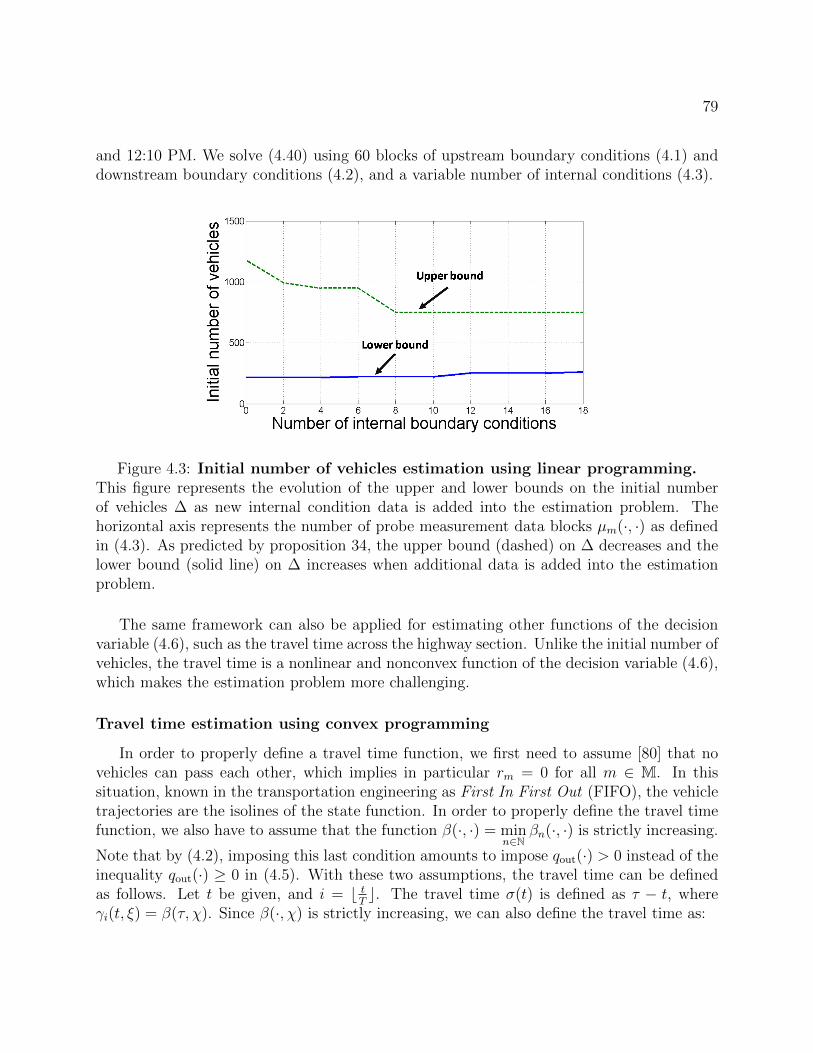
79

and 12:10 PM. We solve (4.40) using 60 blocks of upstream boundary conditions (4.1) anddownstream boundary conditions (4.2), and a variable number of internal conditions (4.3).

Figure 4.3: Initial number of vehicles estimation using linear programming.This figure represents the evolution of the upper and lower bounds on the initial numberof vehicles ∆ as new internal condition data is added into the estimation problem. Thehorizontal axis represents the number of probe measurement data blocks µm(·, ·) as definedin (4.3). As predicted by proposition 34, the upper bound (dashed) on ∆ decreases and thelower bound (solid line) on ∆ increases when additional data is added into the estimationproblem.

The same framework can also be applied for estimating other functions of the decisionvariable (4.6), such as the travel time across the highway section. Unlike the initial number ofvehicles, the travel time is a nonlinear and nonconvex function of the decision variable (4.6),which makes the estimation problem more challenging.

Travel time estimation using convex programming

In order to properly define a travel time function, we first need to assume [80] that novehicles can pass each other, which implies in particular rm = 0 for all m ∈ M. In thissituation, known in the transportation engineering as First In First Out (FIFO), the vehicletrajectories are the isolines of the state function. In order to properly define the travel timefunction, we also have to assume that the function β(·, ·) = min

n∈Nβn(·, ·) is strictly increasing.

Note that by (4.2), imposing this last condition amounts to impose qout(·) > 0 instead of theinequality qout(·) ≥ 0 in (4.5). With these two assumptions, the travel time can be definedas follows. Let t be given, and i = b t

Tc. The travel time σ(t) is defined as τ − t, where

γi(t, ξ) = β(τ, χ). Since β(·, χ) is strictly increasing, we can also define the travel time as:

80

σ(y, t) = mins∈R+ s. t. β(s,χ)≥γi(t,ξ)

(s− t) (4.32)

or alternatively:σ(y, t) = max

s∈R+ s. t. β(s,χ)≤γi(t,ξ)(s− t) (4.33)

Since βj(s, χ) and γi(t, χ) are functions of the decision variable (4.6), the travel timefunction σ(·, ·) hereby defined is a function of the decision variable (4.6), though not linear.While we cannot estimate the travel time using a LP of the form (4.30), we can still obtainvaluable information on upper and lower bounds of the travel time function using LPs, asoutlined in the following proposition.

Proposition 37. [Upper and lower bounds on travel time function] Let us assumethat (4.27) is feasible, that is, the model and data constraints are compatible. Let two timest and τ be given, and let i = b t

Tc and j = b τ

Tc. We have that τ − t is a lower bound on

the travel time σ(y, t) (under the model and data constraints) if and only if the followingproblem is infeasible:

find y

such that

Amodel(ψ)y ≤ bmodel(ψ)Adatay ≤ bdataβj(τ, χ)− γi(t, ξ) ≥ 0

(4.34)

Similarly, τ − t is an upper bound on the travel time σ(y, t) under the model and dataconstraints if and only if the following problem is infeasible:

find y

such that

Amodel(ψ)y ≤ bmodel(ψ)Adatay ≤ bdataβj(τ, χ)− γi(t, ξ) ≤ 0

(4.35)

Proof — We prove that τ − t is a lower bound on the travel time function if andonly if (4.34) is infeasible. Let us assume that (4.34) is infeasible. This amounts to sayingthat βj(τ, χ) < γi(t, ξ) whenever the model and data constraints Amodel(ψ)y ≤ bmodel(ψ)and Adatay ≤ bdata are both satisfied. Hence, since β(τ, χ) = βj(τ, χ) by construction, this isequivalent to saying that β(τ, χ) < γi(t, ξ) whenever the model and data constraints are bothsatisfied. By the definition (4.33) of σ(y, t), this is equivalent to σ(y, t) > τ − t, whenever ysatisfies the model and data constraints, which completes the proof. The proof relative tothe upper bound is similar, and involves the definition (4.32) of σ(y, t). �

Note that the feasibility programs (4.34) and (4.35) enable us to compute the largestlower bound σd(t) and the smallest upper bound σu(t) on the travel time by trial and error.

81

We illustrate the above results by computing the upper and lower bounds on the travel timefunction, using the experimental setup of section 4.1.3, between times 11:40 AM and 12:10PM. For this, we check the feasibility of problems (4.34) and (4.35) for τ = jT , and plotin Figure 4.4 respectively the lowest and highest value of jT such that (4.35) and (4.34)are respectively infeasible. The lowest value jmaxT for which (4.35) is infeasible implies thatσu(t) is in the interval [(jmax − 1)T − t, jmaxT − t]. Similarly, the highest value jminT forwhich (4.34) is infeasible implies that σd(t) is in the interval [jminT − t, (jmin + 1)T − t]. Asstated in proposition 34, the distance between the upper and lower bounds decreases as moredata is added into the estimation problem.

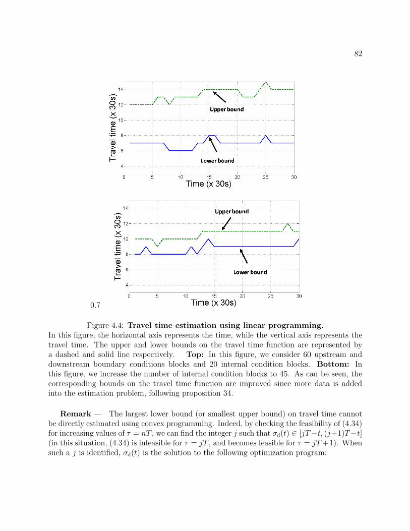
82

0.7

Figure 4.4: Travel time estimation using linear programming.In this figure, the horizontal axis represents the time, while the vertical axis represents thetravel time. The upper and lower bounds on the travel time function are represented bya dashed and solid line respectively. Top: In this figure, we consider 60 upstream anddownstream boundary conditions blocks and 20 internal condition blocks. Bottom: Inthis figure, we increase the number of internal condition blocks to 45. As can be seen, thecorresponding bounds on the travel time function are improved since more data is addedinto the estimation problem, following proposition 34.

Remark — The largest lower bound (or smallest upper bound) on travel time cannotbe directly estimated using convex programming. Indeed, by checking the feasibility of (4.34)for increasing values of τ = nT , we can find the integer j such that σd(t) ∈ [jT−t, (j+1)T−t](in this situation, (4.34) is infeasible for τ = jT , and becomes feasible for τ = jT +1). Whensuch a j is identified, σd(t) is the solution to the following optimization program:

83

minimize zqout(j)

such that

Amodel(ψ)y ≤ bmodel(ψ)Adatay ≤ bdataβj(

zqout(j)

, χ)− γi(t, ξ) ≤ 0

(4.36)

The decision variable of (4.36) can be written as (y, z), where y is the decision variabledefined by (4.6). The constraints Amodel(ψ)y ≤ bmodel(ψ) and Adatay ≤ bdata are both linearin the new decision variable (they indeed depend only upon y). The constraint βj(

zqout(j)

, χ)−γi(t, ξ) ≤ 0 is also linear, since it can be written as:

j−1∑k=0

qout(k)T + qout(j)(z

qout(j)− jT )

−∆−i−1∑k=0

qin(k)T − qin(i)(t− iT ) ≤ 0

(4.37)

The choice of zqout(j)

in the objective function is made to enforce the linearity of the

constraints (and it plays the role of τ in the previous equations). The objective is howevernonconvex, since (z, q) → z

qis not convex. Problem (4.36) thus cannot be solved using

convex programming, but may still be solved numerically using other optimization methods.�

4.5.3 Guaranteed ranges for traffic coefficients estimation

The upper and lower bounds on functions of the decision variable investigated above donot necessarily hold in practice, since the true value y of the decision variable (4.6) may notsatisfy the model and data constraints. However, when the conditions (4.28) hold, the valuesof the upper and lower bounds are guaranteed. Indeed, when (4.28) is satisfied, y belongsto the set {y|Amodel(ψ)y ≤ bmodel(ψ)} ∩ {Adatay ≤ bdata}, which implies

f(y) ≥

minimize f(y)

such that


(4.38)

and

f(y) ≤

maximize f(y)

such that


(4.39)

In order to obtain guaranteed bounds in practice, one has to choose the model parametersuch that the condition (4.28) holds. In the context of traffic flow, the typical values of the

84

model parameter are accurately known, and do not vary significantly between experimentalsites. They are available from [75] for instance. In order to impose (4.28) on all practi-cal traffic scenarios, one simply has to overapproximate these values to define the modelparameters.

4.6 Data assimilation and data reconciliation problems

4.6.1 Problem definition

In the field of distributed parameters system estimation, the problems of data assim-ilation [47] and data reconciliation [37] are closely linked. The data assimilation processconsists in finding the value of the state of the system that satisfies the observations, andthat is the closest to being a solution to the evolution model. In contrast, the data reconcil-iation process consists in finding a solution to the evolution model that is the closest to theobservations. Given the framework detailed above, the data assimilation and reconciliationproblems are related to the solutions of the following convex optimization program.

minimize ||y1 − y2||q

such that

{Amodel(ψ)y1 ≤ bmodel(ψ)Adatay2 ≤ bdata

(4.40)

In the above optimization program, we have to choose q = 1 or q = +∞ to obtain alinear objective. Two situations can arise:

• If the optimal value of (4.40) is 0, the model and data constraints can be satisfied at thesame time. In this situation, the data assimilation and data reconciliation problemscoincide in a setting in which data and model are compatible. The solution is notnecessarily unique.

• If the optimal value of (4.40) is nonzero, the optimal solutions yoptimal1 and yoptimal

2

enable us to compute the upstream, downstream and internal conditions respectivelyassociated with the data reconciliation and data assimilation problems. Note that thesesolutions may not be unique. The value conditions associated with yoptimal

1 satisfy themodel constraints by construction, i.e. all upstream boundary, downstream boundaryand internal conditions blocks apply in the strong sense [8, 13]. They however donot satisfy the data constraints, but are as close as possible in the || · ||q sense to

satisfy them. In contrast, the value conditions associated with yoptimal2 satisfy the data

constraints by construction, but do not satisfy the model constraints (they are as closeas possible to satisfy them in the || · ||q sense).

85

4.6.2 Numerical example

In this application, we consider the spatial domain defined in section 4.1.3, betweenthe times 11:40 AM and 12:05 PM for data collected on February 8th, 2008. We use thefollowing Hamiltonian parameters: kc = 0.048 m−1, v = 24.6 m/s, w = −4.5 m/s, and amaximal relative error level of emax = 0.01. We solve (4.40) for q = 1, using 604 variablesand 17415 linear constraints. For this specific application, the optimal value of (4.40) is+8.58, which ensures that the data assimilation and data reconciliation problems are welldefined. As mentioned above, yoptimal

1 and yoptimal2 enable us to compute the value conditions

associated with the data assimilation and data reconciliation problems. We compute thesolutions to (2.5) associated with these value conditions, and display them in Figure 4.5. Thesolution to the data reconciliation problem at the top of Figure 4.5 satisfies all the boundaryand internal conditions that are prescribed on it. The model applies in the strong sense,however the decision variable violates the data constraints (4.25). In contrast, the upstreamand downstream boundary conditions do not apply everywhere in the solution to the dataassimilation problem (Figure 4.5, center). In the illustrated data assimilation example, thedata constraints some internal conditions to be set in a way that is incompatible with theupstream and downstream boundary conditions. This can be seen for instance around timet = 1100s: a back propagating wave hits the upstream boundary condition at x = 11000m,which prevents it from applying between times t = 1100s and t = 1400s.

86

Figure 4.5: Solutions to data assimilation and data reconciliation problems.Top: Solution to the data reconciliation problem, in which the model constraints are satis-

fied, but the data constraints are not. Center: Solution to the data assimilation problem,in which the data constraints are satisfied, but the model constraints are not. Both problemsare solved simultaneously by (4.40). Bottom: Difference (in number of vehicles) betweenthe solution to the data reconciliation problem and the solution to the data assimilationproblem.

87

4.7 Cybersecurity, sensor fault detection and privacy

analysis problems

4.7.1 Consistency problems applied to sensor failure detection

The framework developed in section 4.4 can also be applied to detect failures in sensornetworks. In this section, we are interested in checking the consistency of the data generatedby sensors of the PeMS system [103], which is a network of loop detectors measuring trafficon California highways. The PeMS system is one of the data feeds currently integrated inthe Mobile Millennium traffic monitoring system [98, 101], operated jointly by Nokia andUC Berkeley. One of the main challenges arising when using data from the PeMS system isthe automated identification of the mislocated or faulty sensors. Previous approaches suchas [67] have successfully implemented sensor fault detection algorithms based on statisticalcorrelation with adjacent sensors. Our approach is different though, since it can guaranteeusing the PDE model that at least one of the sensors in an array of sensors is failing.

We solve the fault detection problem either by checking the feasibility of the consistencyproblem (4.27) using a Hamiltonian satisfying (4.28) on all pairs of consecutive sensorspresent on the highway network.

We assume that the maximal allowable error of a PeMS sensor is emax = 0.3 in (4.23).There are multiple sources of uncertainty arising when dealing with loop detectors, such aspavement depth, loop layout, which typically creates maximal errors of this magnitude. Wealso choose an Hamiltonian ψ(·) satisfying (4.28) by overapproximating the tabulated valuesof [75]: kc = 0.05 m−1, v = 30 m/s, w = −7 m/s.

As an application, we consider five consecutive PeMS sensors, labeled 401339, 401714,401376, 400609 and 400835 respectively, as illustrated in Figure 4.6. For each one of thefour adjacent pairs of sensors, we compute the minimal value of the error emax such that theconsistency problem (4.27) is feasible during a one month period at the frequency of one day.The distribution of these results is shown in Figure 4.6. Note that since emax appears linearlyin the data constraints, the minimal value of the error emax such that (4.27) is feasible is alsoa LP.

Figure 4.6 shows that there is no indication of malfunction for the first and the last pairsof sensors. Note that the success to the minimal error test does not guarantee that a pairof sensors is working, since the actual error of the pair of sensors can be above the maximalallowable error.

The second and third pairs exhibit errors that are higher than 0.3, which indicates amalfunction of the corresponding pairs. Further analysis has shown that the pair 401714−400609 is passing the minimal error test and thus that sensor 401376 is likely incorrectlymapped.

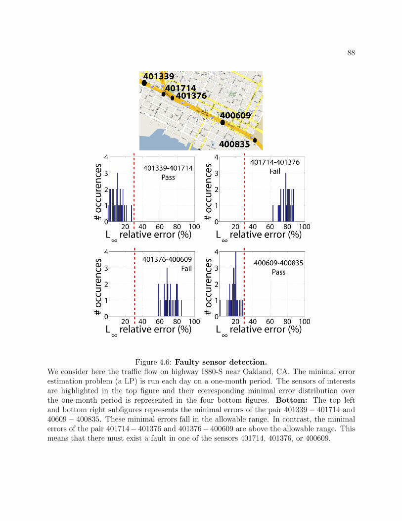
88

Figure 4.6: Faulty sensor detection.We consider here the traffic flow on highway I880-S near Oakland, CA. The minimal errorestimation problem (a LP) is run each day on a one-month period. The sensors of interestsare highlighted in the top figure and their corresponding minimal error distribution overthe one-month period is represented in the four bottom figures. Bottom: The top leftand bottom right subfigures represents the minimal errors of the pair 401339− 401714 and40609− 400835. These minimal errors fall in the allowable range. In contrast, the minimalerrors of the pair 401714− 401376 and 401376− 400609 are above the allowable range. Thismeans that there must exist a fault in one of the sensors 401714, 401376, or 400609.

89

4.7.2 Consistency problems applied to cybersecurity

One type of cyberattack [4] consists in faking sensor data and sending it to the monitoringsystem as if it was originating from valid sensors. Detecting this form of cyberattack is acomplex problem in general. Detecting fake data that follows some pattern (for instance ifthe faked data is periodic) or that falls out of physically reasonable bounds is easy. However,detecting fake data that is both random and consistent with the expected value of sensormeasurements is difficult.

A possible approach for solving this problem is to check if (4.27) is feasible, under theassumption (4.28). If (4.27) is feasible, this implies that the data is consistent with ourmodel and data assumptions. Note that this does not guarantee that no cyberattack occurs.Indeed, an attacker can send fake data in a way that is consistent with the model and errorlevels assumptions. However, if (4.27) is infeasible, at least one of the assumptions (4.28)is false. Either the Hamiltonian does not satisfy (4.28), or the error model (4.28) is wrong.Any of these two situations can denote a cyber-attack if the conditions (4.28) are known tohold. However, note that other phenomena such as sensor failures can also cause (4.27) tobe infeasible. The same framework can be applied to sensor fault detection.

We illustrate the cyberattack detection method (4.27) by simulating an attacker sendingfake random values of xmin(·), xmax(·), tmin(·) and tmax(·), leading to the construction of newfake internal conditions using (4.3). The values of xmin(·), xmax(·), tmin(·) and tmax(·) are cho-

sen randomly as follows. The speed xmax(·)−xmin(·)tmax(·)−tmin(·) associated with the internal condition is

chosen uniformly in an interval [vmin, vmax]. The coefficients satisfy xmin(·) ≥ ξ, xmax(·) ≤ χ,tmin(·) ≥ 0 and tmax(·) ≤ nmaxT . In the numerical applications, we consider the experimentalsetup described in section 4.1.3, between times 11:40 AM and 12:00 PM. We use 30 exper-imental internal conditions (4.3), 40 experimental upstream boundary conditions (4.1) and40 experimental downstream boundary conditions (4.2). We progressively add fake internalconditions (4.3) and solve problem (4.40) for q = 1, and for a Hamiltonian satisfying (4.28).Note that (4.27) is feasible if and only if the solution to (4.40) is zero. Thus, the solutionto (4.40) is a measure of the “distance” or incompatibility between data and model. In orderto facilitate comparisons and reproduce the results, each result in Figure 4.7 top and bottomwas averaged over 10 different choices of fake internal conditions.

As illustrated in Figure 4.7 top, adding fake speed measurements increases the incom-patibility between data and model. The incompatibility between data and model is 0 whenno fake measurements are added, which is consistent with the fact that (4.28) holds. Notethat adding fake speeds does not have a significant impact on the level of incompatibilitybetween data and model when the fake speeds are close to the average speed on the highwaysection (20 mph in this experiment) which is also consistent with the physics of the problem.

Figure 4.7 bottom shows that the configuration of the measurement data plays a criticalrole. In this figure, we study the influence of the measurement data on the detection ofcyberattacks. For this, we consider four different subsets of 30 internal conditions each,extracted from our measurement data. An example of subset of 12 internal conditions among

90

28 available measurements is illustrated in Figure 4.8. We fix the fake speeds range to [30mph, 35 mph], and show the solution to (4.27) for these four configurations, represented onthe horizontal axis. As can be seen from this figure, depending on the configuration of ourmeasurement data, we can have very different ranges of level of incompatibility between dataand model, for identical number of actual measurements, number of fake internal conditionsand range of fake speeds. In the configurations ]1 and ]4, it is very difficult to detect that aspoofing attack occurs, since no change in the optimal value of (4.40). However, the spoofingattack is easily detected in the configuration ]2, even though all configurations contain thesame amount of measurement data. These results thus show that it is almost impossibleto determine if detecting a cyberattack is easy based on the amount of measurement dataalone.

4.7.3 Privacy analysis problems

Another possible application of the framework defined in section 4.5 is the analysis ofuser privacy using linear programming. The label of the vehicle represented by the internalcondition µm(·, ·) defined by (4.3) is Lm. In practical problems, the same vehicle sendsdifferent packets of information, representing different internal conditions (4.3). To whatextent is it possible to “reidentify” one vehicle, i.e. to track it by identifying the pieces ofdata that came from the same vehicle?

Standard methods [60] do not take into account the model constraints: they usuallytry to reidentify vehicles under the assumption that vehicles maintain a relatively constantspeed. While this is true for a large number of traffic scenarios, it does not take into accountthe underlying model, and can fail if the the traffic speeds change significantly through thecomputational domain.

If we assume that vehicles do not pass each other (this implies rm = 0 for all m ∈ M),the minimal and maximal number of vehicles between two different internal condition blocksµi(·, ·) and µj(·, ·) is solution to the following LP:

minimize (or maximize) |Li − Lj|

such that

Amodel(ψ)y ≤ bmodel(ψ)Adatay ≤ bdatarm = 0 ∀m ∈M

(4.41)

The above LP enables us to identify situations in which the privacy of users could bebreached. Indeed, when the maximal number of vehicles between µi(·, ·) and µj(·, ·) is zero,these boundary conditions represent the same vehicle. In contrast, when the minimal numberof vehicles between µi(·, ·) and µj(·, ·) is nonzero, these boundary conditions cannot originatefrom the same vehicle. We thus have three cases:

91

1. If the optimal value |Li−Lj|max of the maximization problem (4.41) is zero, then µi(·, ·)and µj(·, ·) have been generated by the same vehicle.

2. If the optimal value |Li − Lj|min of the minimization problem (4.41) is nonzero, thenµi(·, ·) and µj(·, ·) cannot have been generated from the same vehicle.

3. Other cases are inconclusive

We show an example of vehicle reidentification in Figure 4.9, using the experimentalsetup of section 4.1.3.

In practical computations, given an internal condition µi(·, ·), there may exist multiplej ∈ M such that the solution to the minimization problem (4.41) is zero. If this happen,we lost track of vehicle i, which can be desirable in the context of traffic flow engineering(see [60] for an analysis of user privacy in mobile traffic sensing systems).

92

Figure 4.7: Cyberattack detection using linear programming.In these figures, we represent the solution to (4.40) as a color map. Low values are representedas dark areas, and correspond to situations in which the “compatibility” between model anddata is “good”, i.e. lower values of ||y2− yi|| in (4.27). High values are represented as light-colored areas, and denote a higher degree of incompatibility between the model and dataconstraints. Top: The horizontal axis in this figure represents the lower bound k of theinterval [k mph, k+5 mph] in which the fake speed data is drawn. The vertical axis representsthe number of fake internal conditions added. For instance, the cell (15, 12) corresponds to12 fake internal conditions for which the speed is in the interval [15 mph, 20 mph]. As canbe seen from this figure, the distance increases when more fake measurements are added intothe estimation problem, and when they correspond to a speed that is far away from the trueaverage speed (around 20 mph in this application). Bottom: This figure illustrates the highsensitivity of the solution to (4.40) with respect to the available measurement data. In thisfigure, we consider four different sets of 30 actual internal boundary conditions each. Theprocedure used for choosing a random subset of the available measurement data is illustratedin Figure 4.8. For each of these subsets (configurations), we add an increasing quantity offake internal conditions, associated with random speeds ranging in [30 mph, 35 mph]. Ascan be seen, the results vary dramatically depending on which subset of the available datawas chosen, even if the number of fake internal conditions is identical.

93

Figure 4.8: Illustration of the choice of a subset of measurement data.In this figure, each segment represents the domain of an internal condition (4.3), obtainedusing experimental data. We illustrate the choice of two subsets of 12 internal conditionsamong 28 speed measurements, which we call “configuration”. The same process applies forFigure 4.7, bottom, with four different configurations involving 30 internal conditions eachamong 94 available speed measurements.

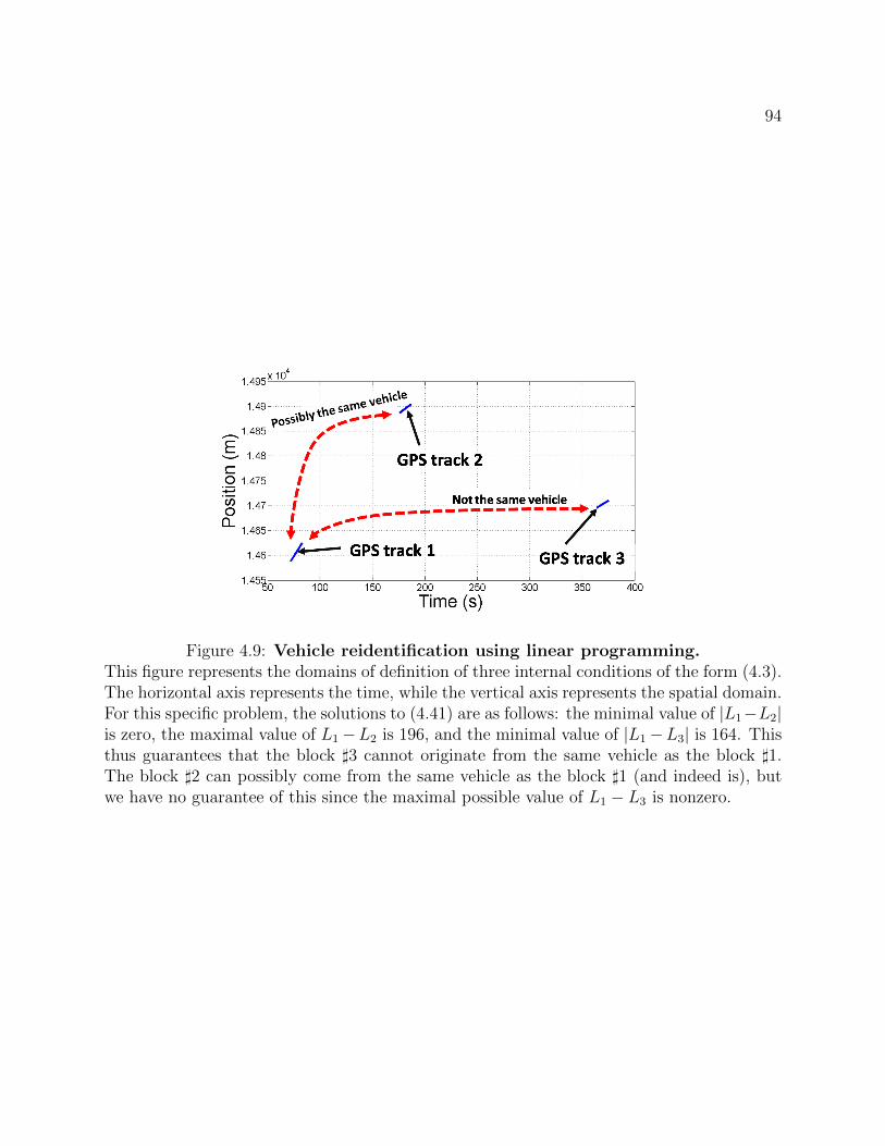
94

Figure 4.9: Vehicle reidentification using linear programming.This figure represents the domains of definition of three internal conditions of the form (4.3).The horizontal axis represents the time, while the vertical axis represents the spatial domain.For this specific problem, the solutions to (4.41) are as follows: the minimal value of |L1−L2|is zero, the maximal value of L1−L2 is 196, and the minimal value of |L1−L3| is 164. Thisthus guarantees that the block ]3 cannot originate from the same vehicle as the block ]1.The block ]2 can possibly come from the same vehicle as the block ]1 (and indeed is), butwe have no guarantee of this since the maximal possible value of L1 − L3 is nonzero.

95

Chapter 5

Conclusion

5.1 Contributions

This dissertation presented a new computational method for solving the Hamilton Ja-cobi (HJ) partial differential equation (PDE), as well as a new convex optimization-basedestimation framework based on this computational method. Using the control frameworkof viability theory, we characterized the solutions to the HJ PDE by a Lax-Hopf formulaand derived an important inf-morphism property. With these properties, we showed thatthe solution associated with piecewise affine initial, boundary and internal conditions can becomputed as the minimum of solutions associated with affine initial, boundary and internalconditions. We then showed that the later can be computed explicitly, which enables theconstruction of a semi-analytic numerical scheme for computing the solutions to HJ PDEs.The key advantages of this numerical scheme over standard computational methods are itsexactness and fast computational speed.

The semi-explicit expression of the solutions enabled us to derive the HJ PDE modelconstraints explicitly. Using the Lax-Hopf formula, we proved that these model constraintsare convex. Given that the measurement data constraints are also convex, a large number ofestimation problems for which the model is a HJ PDE can be posed as convex-optimizationprograms. We presented various practical applications of this framework, which were im-plemented as Linear Programs. Numerical applications using experimental data sets wereperformed.

Some of the estimation problems developed in this thesis have been implemented in theMobile Millennium system, a real-time traffic flow monitoring system operated jointly byUC Berkeley and Nokia. The main application of this framework to Mobile Millennium hasbeen the detection of faulty sensors. For this specific application, a set of algorithms runsin real time and checks the consistency of the data generated by more than 2000 sensors inNorthern California every 30 seconds. These algorithms have already identified a numberof faulty and misplaced sensors, which enables the Mobile Millennium system to run faster

96

and with greater confidence.

5.2 Open problems

5.2.1 Mathematical problems

Numerous mathematical and computational problems remain for the general problem ofcontrol and estimation of highway networks. The extension of this framework to the highwaynetwork as a whole is a very complex problem. Indeed, in networks, the boundary conditionsof each computational domain are not necessarily known because sensors are not necessarilylocated at the edge of each link. Hence, while we assumed that the boundary conditions ofthe computational domain were known in the numerical examples presented in this thesis,this assumption is not necessarily satisfied in practice. In addition, the coupling betweenlinks induces additional mathematical difficulties when relating the model compatibility con-straints from link to link. This is a major problem, which only has a partial solution in thecase of LWR PDEs [53], and is still open for HJ PDEs.

The framework presented above could also be extended for the case in which we con-sider the viscosity solutions to the HJ PDE. While Barron-Jensen/Frankowska solutions andviscosity solutions to Hamilton-Jacobi equations can be shown to be equivalent for Lipschitz-continuous initial and boundary conditions, they differ when internal boundary conditionsare present. In this case, the solution associated with the scalar conservation counterpart ofthe HJ PDE is the derivative of the viscosity (and not the B-J/F) solution of the HJ PDE.Hence, in order to extend this estimation framework to scalar conservation laws, one needsto derive the model compatibility constraints for viscosity solutions, which differ from themodel constraints established in this dissertation. This extension would enable the estima-tion of quantities related to the density and flow functions, which are more easily observedthan their integrals (the Moskowitz function).

Finally, the explicit mathematical link between weak boundary conditions in HJ PDEsand weak boundary conditions of the associated conservation laws is still not established.Neither is the proper functional space requirement needed to unify both theories.

5.2.2 Application problems

This framework has yet to be extended to other traffic estimation problems, such as queuelength estimation, which is of great interest for traffic estimation in urban environments.These problems are usually driven by the periodic forcing of the boundary conditions bytraffic lights or stop signs which results in periodic behavior of the flow. Solving suchproblems requires the identification of free-flow and congested areas, which is usually difficultsince it involves the derivatives of the Moskowitz function. Thus, the resulting problemswould be non-convex by nature, but may still be computationally tractable. Also, by nature

97

of the problem, shock waves appear periodically, which need to be incorporated in themethod.

5.3 Future work

Future work will be first dedicated to extending the framework presented in this thesisto systems modeled by conservation laws. Preliminary analysis shows that if we consider theviscosity solutions to the HJ PDE, the resulting model compatibility constraints become non-convex, and the estimation problems take the general form of mixed integer linear programs(MILPs). MILPs are significantly harder to solve than LPs, but may still be tractable inreal time for specific systems.

Estimation on general highway networks will be the second focus, in particular the prob-lem of integrating a set of boundary condition constraints into the estimation problem. Thestate of networked highway sections is more complex to estimate, since the sections interactat their respective boundaries. Hence, the estimation of the state of traffic on the highwaynetwork cannot be decoupled into separate traffic estimation problems on highway sections.Integrating the boundary condition constraints between sections into the respective estima-tion problems yields a non-convex problem. Again, this problem may still be decomposedinto a series of convex problems.

Finally, a promising avenue is to study how flow models can enable us to better esti-mate pollution levels in urban environments. While pollution can be directly measured andmapped, the integration of traffic flow estimates (with traffic flow emission models) intothe problem of estimating urban pollution will improve the quality of the estimation. Thisproblem is mathematically very challenging because of the coupling of both phenomena. Itwill however open the door to traffic flow control for controlling pollution levels in urbanenvironment to safe limits.

98

Bibliography

[1] O. M. Aamo, A. Smyshlyaev, P. Rouchon, and P. Martin. Boundary control ofa nonlinear Stefan problem. In Proceedings of the IEEE Conference on Decision andControl, pages 1309–1314, Maui, HI, Dec. 2003.

[2] P. Abbeel and A. Y. Ng. Apprenticeship learning via inverse reinforcement learning.In Proceedings of the twenty-first international conference on Machine learning, page 1.ACM, 2004.

[3] L. Alvarez-Icaza, L. Munoz, X. Sun, and R. Horowitz. Adaptive observer fortraffic density estimation. In Proceedings of the American Control Conference, pages2705–2710, Boston, MA, June 2004.

[4] S. Amin, A. Cardenas, and S. Sastry. Safe and Secure Networked Control Systemsunder Denial-of-Service Attacks. Number 5469 in Lecture Notes in Computer Science,pages 31–45. Springer, San Francisco, CA, 2009.

[5] R. Ansorge. What does the entropy condition mean in traffic flow theory? Trans-portation Research, 24B(2):133–143, 1990.

[6] J.-P. Aubin. Viability Theory. Systems and Control: Foundations and Applications.Birkhauser, Boston, MA, 1991.

[7] J.-P. Aubin. Viability kernels and capture basins of sets under differential inclusions.SIAM Journal of Control and Optimization, 40:853–881, 2001.

[8] J.-P. Aubin, A. M. Bayen, and P. Saint-Pierre. Dirichlet problems for someHamilton-Jacobi equations with inequality constraints. SIAM Journal on Control andOptimization, 47(5):2348–2380, 2008. Also available as a technical report, Preprint diMathematica - n. 4, Scuola Normale Superiore, Pisa, Italy, May, 2006.

[9] J.-P. Aubin and A. Cellina. Differential inclusions. Springer-Verlag, New York, NY,1984.

[10] J.-P. Aubin and H Frankowska. Set Valued Analysis. Birkhauser, Boston, MA,1990.

99

[11] A. Aw and M. Rascle. Resurrection of “second order” models of traffic flow. SIAMjournal on applied mathematics, 60(3):916–938, 2000.

[12] M. Bardi and I. Capuzzo-Dolcetta. Optimal Control and Viscosity Solutions ofHamilton-Jacobi-Bellman equations. Birkhauser, Boston, MA, 1997.

[13] C. Bardos, A. Y. Leroux, and J. C. Nedelec. First order quasilinear equationswith boundary conditions. Communications in partial differential equations, 4(9):1017–1034, 1979.

[14] E. N. Barron and R. Jensen. Semicontinuous viscosity solutions for Hamilton-Jacobi equations with convex Hamiltonians. Comm. Partial Differential Equations,15:1713–1742, 1990.

[15] Y. Bar-Shalom, X.R. Li, and T. Kirubarajan. Estimation with applications totracking and navigation. Wiley-Interscience, 2001.

[16] A. M. Bayen, R. L. Raffard, and C. Tomlin. Network congestion alleviation usingadjoint hybrid control: Application to highways. Number 1790 in Lecture Notes inComputer Science, pages 95–110. Springer Verlag, 2004.

[17] S. Blandin, D. Work, P. Goatin, B. Piccoli, and A. Bayen. A general phasetransition model for vehicular traffic. Preprint, 2009.

[18] S. Boyd and L. Vandenberghe. Convex Optimization. Cambridge University Press,Cambridge, UK, 2004.

[19] A. Bressan. Hyperbolic systems of conservation laws: the one dimensional Cauchyproblem. Oxford Lecture Series in Mathematics and its Applications, 20. Oxford Uni-versity Press, Oxford, UK, 2000.

[20] A. Bressan, G. Crasta, and B. Piccoli. Well-posedness of the Cauchy problem fornxn systems of conservation laws. American Mathematical Society, 2000.

[21] W. Burghout. Hybrid microscopic-mesoscopic traffic simulation. Royal Institute ofTechnology Doctoral Dissertation, 2004.

[22] P. Cardaliaguet, M. Quincampoix, and P. Saint-Pierre. Optimal times for con-strained nonlinear control problems without local controllability. Applied Mathematicsand Optimization, 36:21–42, 1997.

[23] P. Cardaliaguet, M. Quincampoix, and P. Saint-Pierre. Set-valued numeri-cal analysis for optimal control and differential games. In M. Bardi, T.E.S. Raghavan,and T. Parthasarathy, editors, Stochastic and Differential Games: Theory and Numer-ical Methods, Annals of the International Society of Dynamic Games, pages 177–247.Birkhauser, 1999.

100

[24] S. Y. Cheung, S. C. Ergen, and P. Varaiya. Traffic surveillance with wirelessmagnetic sensors. In Proceedings of the 12th ITS World Congress, 2005.

[25] A. J. Chorin. Numerical solution of Boltzmann’s equation. Communications on Pureand Applied Mathematics, 25(2):171–186, 1972.

[26] A. J. Chorin and X. Tu. Implicit sampling for particle filters. Proceedings of theNational Academy of Sciences, 106(41):17249, 2009.

[27] P. D. Christofides. Nonlinear and robust control of PDE systems: methods andapplications to transport-reaction processes. Birkhauser, 2001.

[28] P. H. Clarke, Y. S. Ledyaev, R. J. Stern, and P. R. Wolenski. Qualitativeproperties of trajectories of control systems: a survey. Journal of dynamical andcontrol systems, 1(1):1–48, 1995.

[29] C. G. Claudel and A. M. Bayen. Solutions to switched Hamilton-Jacobi equationsand conservation laws using hybrid components. Number 4981 in Lecture Notes inComputer Science, pages 101–115. Springer Verlag, Saint Louis, MO, 2008.

[30] C. G. Claudel and A. M. Bayen. Convex formulations of data assimilation problemsfor a class of Hamilton-Jacobi equations. Submitted to SIAM Journal on Control andOptimization, 2009.

[31] C. G. Claudel and A. M. Bayen. Lax-Hopf based incorporation of internal bound-ary conditions into Hamilton-Jacobi equation. Part I: theory. IEEE Transactions onAutomatic Control, 55(5):1142–1157, 2010. doi:10.1109/TAC.2010.2041976.

[32] C. G. Claudel and A. M. Bayen. Lax-Hopf based incorporation of inter-nal boundary conditions into Hamilton-Jacobi equation. Part II: Computationalmethods. IEEE Transactions on Automatic Control, 55(5):1158–1174, 2010.doi:10.1109/TAC.2010.2045439.

[33] R. M. Colombo. Hyperbolic phase transitions in traffic flow. SIAM Journal onApplied Mathematics, 63(2):708–721, 2002.

[34] J. M. Coron, B. d’Andrea-Novel, and G. Bastin. A strict Lyapunov functionfor boundary control of hypebolic systems of conservation laws. In Proceedings of theAmerican Control Conference, pages 3319–3323, Paradise Island, Bahamas, Dec. 2004.

[35] M. G. Crandall, L. C. Evans, and P.-L. Lions. Some properties of viscosity so-lutions of Hamilton-Jacobi equations. Transactions of the American MathematicalSociety, 282(2):487–502, 1984.

101

[36] M. G. Crandall and P.-L. Lions. Viscosity solutions of Hamilton-Jacobi equations.Transactions of the American Mathematical Society, 277(1):1–42, 1983.

[37] C. M. Crowe. Data reconciliation-progress and challenges. Journal of Process Control,6(2):89–98, 1996.

[38] C. M. Dafermos. Polygonal approximations of solutions of the initial value problemfor a conservation law. Journal of Mathematical Analysis and Applications, 38(1):33–41, 1972.

[39] C. Daganzo. The cell transmission model: a dynamic representation of highway trafficconsistent with the hydrodynamic theory. Transportation Research, 28B(4):269–287,1994.

[40] C. Daganzo. The cell transmission model, part II: network traffic. TransportationResearch, 29B(2):79–93, 1995.

[41] C. Daganzo. A variational formulation of kinematic waves: basic theory and complexboundary conditions. Transporation Research B, 39B(2):187–196, 2005.

[42] C. Daganzo. On the variational theory of traffic flow: well-posedness, duality andapplications. Networks and Heterogeneous Media, 1:601–619, 2006.

[43] A. Downs. Still stuck in traffic: coping with peak-hour traffic congestion. BrookingsInst Pr, 2004.

[44] L. C. Evans. Partial Differential Equations. Graduate Studies in Mathematics. Amer-ican Mathematical Society, Providence, RI, 1998.

[45] L. C. Evans and P. E. Souganidis. Differential games and representation formulasfor solutions of Hamilton-Jacobi-Isaacs equations. Indiana University MathematicsJournal, 33(5):773–797, 1984.

[46] G. Evensen. Using the extended Kalman filter with a multilayer quasi-geostrophicocean model. Journal of Geophysical Research, 97(C11):17905–17924, 1992.

[47] G. Evensen. Data Assimilation: The Ensemble Kalman Filter. Springer-Verlag,Berlin Heidelberg, Germany, 2007.

[48] M. Falcone and R. Ferretti. Semi-Lagrangian schemes for Hamilton-Jacobi equa-tions, discrete representation formulae and Godunov methods. Journal of computa-tional physics, 175(2):559–575, 2002.

[49] M. Fliess, J. Levine, P. Martin, and P. Rouchon. Flatness and defect of non-linear systems: introductory theory and examples. International Journal of Control,61(6):1327–1361, 1995.

102

[50] M. Fliess, P. Martin, N. Petit, and P. Rouchon. Active signal restoration for thetelegraph equation. In IEEE Conference on Decision and Control, volume 2, pages1107–1111, 1999.

[51] G. F.Newell. A simplified car-following theory: a lower order model. TransportationResearch Part B: Methodological, 36(3):195–205, 2002.

[52] H. Frankowska. Lower Semicontinuous Solutions of Hamilton-Jacobi-Bellman Equa-tions. SIAM Journal of Control and Optimization, 31(1):257–272, 1993.

[53] M. Garavello and B. Piccoli. Traffic flow on networks. American Institute ofMathematical Sciences, Springfield, MO, USA, 2006.

[54] S. K. Godunov. A difference method for numerical calculation of discontinuous solu-tions of the equations of hydrodynamics. Math. Sbornik, 47:271–306, 1959.

[55] M. Grant and S. Boyd. CVX: Matlab software for disciplined convex programming,version 1.21. http://cvxr.com/cvx, July 2010.

[56] B. D. Greenshields. A study of traffic capacity. Proceedings of the Highway ResearchBoard, 14:448–477, 1935.

[57] J. C. Herrera, D. B. Work, R. Herring, X. J. Ban, Q. Jacobson, and A. M.Bayen. Evaluation of traffic data obtained via GPS-enabled mobile phones: The Mo-bile Century field experiment. Transportation Research Part C: Emerging Technologies,18:568–583, 2010.

[58] J.C. Herrera and A.M. Bayen. Incorporation of Lagrangian measurements infreeway traffic state estimation. Transportation Research Part B: Methodological,44(4):460–481, May 2010.

[59] R. Herring, A. Hofleitner, P. Abbeel, and A. M. Bayen. Estimating arterialtraffic conditions using sparse probe data. In Proceedings of the 13th InternationalIEEE Conference on Intelligent Transportation Systems, Madeira Island, Portugal,2010.

[60] B. Hoh, M. Gruteser, R. Herring, J. Ban, D. Work, J. C. Herrera, A. M.Bayen, M. Annavaram, and Q. Jacobson. Virtual trip lines for distributed privacy-preserving traffic monitoring. In MobiSys, Breckenridge, CO, June 2008.

[61] H. Holden and N.H. Risebro. Front tracking for hyperbolic conservation laws.Springer Verlag, New York, N.Y., 2002.

[62] P. L. Houtekamer and H. L. Mitchell. A sequential ensemble Kalman filter foratmospheric data assimilation. Monthly Weather Review, 129:123–137, 2001.

103

[63] T. Hunter, R. Herring, P. Abbeel, and A.M. Bayen. Path and travel timeinference from GPS probe vehicle data. In Proceedings of the Neural InformationProcessing Systems foundation (NIPS), Vancouver, Canada, 2009.

[64] C. Y. Kao, S. Osher, and J. Qian. Lax-Friedrichs sweeping scheme for staticHamilton-Jacobi equations. Journal of Computational Physics, 196(1):367–391, 2004.

[65] M. Krstic and A. Smyshlyaev. Adaptive boundary control for unstable parabolicPDEs. Part I: Lyapunov design. IEEE Transactions on Automatic Control, 53(7):1575,2008.

[66] M. Krstic and A. Smyshlyaev. Backstepping boundary control for first-order hy-perbolic PDEs and application to systems with actuator and sensor delays. Systems& Control Letters, 57(9):750–758, 2008.

[67] J. Kwon, C. Chen, and P. Varaiya. Statistical methods for detecting spatial config-uration errors in traffic surveillance sensors. Transportation Research Record: Journalof the Transportation Research Board, 1870(1):124–132, 2004.

[68] P. D. Lax. Hyperbolic systems of conservation laws II. Selected Papers Volume I,pages 233–262, 2005.

[69] L. Leclercq. Bounded acceleration close to fixed and moving bottlenecks. Trans-portation research. Part B: methodological, 41(3):309–319, 2007.

[70] P. Le Floch. Explicit formula for scalar non-linear conservation laws with boudarycondition. Mathematical Methods in the Applied Sciences, 10:265–287, 1988.

[71] R. LeVeque. Numerical methods for conservation laws. Birkhauser, Basel, Switzer-land, 1992.

[72] M. J. Lighthill and G. B. Whitham. On kinematic waves. II. A theory of traffic flowon long crowded roads. Proceedings of the Royal Society of London, 229(1178):317–345,1956.

[73] X. Litrico. Robust flow control of single input multiple outputs regulated rivers.Journal of Irrigation and Drainage Engineering, 127(5):281–286, 2001.

[74] X. Litrico and V. Fromion. Boundary control of linearized saint-venant equationsoscillating modes. In Proceedings of the American Control Conference, pages 2131–2136, Paradise Island, Bahamas, Dec. 2004.

[75] Highway Capacity Manual. Special report 209. Transportation Research Board, Wash-ington, DC, 1985.

104

[76] I. Mitchell. A toolbox of level set methods. http://www.cs.ubc.ca/ mitchell,2005.

[77] I. Mitchell. Games of two identical vehicles. Technical Report SUDAAR 740, De-partment of Aeronautics and Astronautics, Stanford University, Stanford, CA, July2001.

[78] I. M. Mitchell, A. M. Bayen, and C. J. Tomlin. Computing reachable sets forcontinuous dynamic games using level set methods. IEEE Transactions on AutomaticControl, 50(7):947–957, 2005.

[79] K. Moskowitz. Discussion of ‘freeway level of service as influenced by volume andcapacity characteristics’ by D.R. Drew and C. J. Keese. Highway Research Record,99:43–44, 1965.

[80] G. F. Newell. A simplified theory of kinematic waves in highway traffic. Transpora-tion Research B, 27B(4):281–303, 1993.

[81] M. Papageorgiou. Some remarks on macroscopic traffic flow modelling. Transporta-tion Research Part A: Policy and Practice, 32(5):323–329, 1998.

[82] N. Petit. Delay Systems. Flatness in Process Control and Control of some Wave Equa-tions. PhD thesis, Ecole des Mines de Paris, Centre d’Automatique et des Systemes,Paris, France, 2000.

[83] L.A. Pipes. Car following models and the fundamental diagram of road traffic. Trans-portation Research, 1(1):21–29, 1967.

[84] C. Prieur and J. de Halleux. Stabilization of a 1-D tank containing a fluid modeledby the shallow water equations. Systems & Control Letters, 52(3-4):167–178, 2004.

[85] T.S. Rabbani, F. Di Meglio, X. Litrico, and A.M. Bayen. Feed-forward controlof open channel flow using differential flatness. IEEE Transactions on Control SystemsTechnology, 18(1):213–221, 2009.

[86] P. I. Richards. Shock waves on the highway. Operations Research, 4(1):42–51, 1956.

[87] R.T. Rockafellar. Convex Analysis. Princeton University Press, 1970.

[88] P. Saint-Pierre. Approximation of the viability kernel. Applied Mathematics andOptimization, 29:187–209, 1994.

[89] J. A. Sethian. Level Set Methods and Fast Marching Methods. Cambridge UniversityPress, New York, NY, 1999.

105

[90] R. C. Smith and M. A. Demetriou. Research Directions in Distributed ParameterSystems. SIAM, Philadelphia, PA, 2000.

[91] I. S. Strub and A. M. Bayen. Weak formulation of boundary conditions for scalarconservation laws. International Journal of Robust and Nonlinear Control, 16:733–748,2006.

[92] D. Sun and A. M. Bayen. Multicommodity Eulerian-Lagrangian large-capacity celltransmission model for en route traffic. Journal of Guidance Control and Dynamics,31(3):616, 2008.

[93] X. Sun, L. Munoz, and R. Horowitz. Methodological calibration of the cell trans-mission model. In Proceedings of the American Control Conference, Boston, MA, June2004.

[94] O. P. Tossavainen, J. Percelay, A. Tinka, Q. Wu, and A.M. Bayen. Ensemblekalman filter based state estimation in 2d shallow water equations using lagrangiansensing and state augmentation. In 47th IEEE Conference on Decision and Control,2008, pages 1783–1790, 2008.

[95] P. Varaiya. Reducing highway congestion: an empirical approach. European Journalof Control, 11(4-5), 2005.

[96] Y. Wang and M. Papageorgiou. Real-time freeway traffic state estimation basedon extended Kalman filter: a general approach. Transportation Research Part B:Methodological, 39(2):141–167, 2005.

[97] D. Work, S. Blandin, O. Tossavainen, B. Piccoli, and A. Bayen. A distributedhighway velocity model for traffic state reconstruction. Applied Research MathematicseXpress (ARMX), 1:1–35, April 2010.

[98] D. Work, O.P. Tossavainen, S. Blandin, A. Bayen, T. Iwuchukwu, andK. Tracton. An ensemble Kalman filtering approach to highway traffic estimationusing GPS enabled mobile devices. In Proceedings of the 47th IEEE Conference onDecision and Control, pages 2141–2147, Cancun, Mexico, December 2008.

[99] Q. Wu, X. Litrico, and A. M. Bayen. Data reconciliation of an open channel flownetwork using modal decomposition. Advances in Water Resources, 32(2):193–204,2009.

[100] H. M. Zhang. A theory of nonequilibrium traffic flow. Transportation Research PartB: Methodological, 32(7):485–498, 1998.

[101] http://traffic.berkeley.edu/.

106

[102] http://www.ngsim.fhwa.dot.gov/.

[103] http://pems.eecs.berkeley.edu.

Convex formulations of inverse modeling problems on ...

Documents

Transcript of Convex formulations of inverse modeling problems on ...