Converted-wave moveout and conversion-point equations … · Converted-wave moveout and...

www.elsevier.com/locate/jappgeo

Journal of Applied Geophysics 54 (2003) 297–318

Converted-wave moveout and conversion-point equations in

layered VTI media: theory and applications

Xiang-Yang Lia,*, Jianxin Yuanb

aBritish Geological Survey, West Mains Road, Edinburgh EH9 3LA, Scotland, UKbPGS Inc., 10550 Richmond Avenue, Suite 300, Houston, TX 77042, USA

Abstract

We have developed improved equations for calculating the conversion point of the P-SV converted wave (C-wave) in

transversely isotropic media with a vertical symmetry axis (vertical transverse isotropy (VTI)). We have also derived modified

C-wave moveout equations for layered VTI media. The derived equations for the conversion-point are valid for offsets about

three-times the reflector depth (x/z= 3.0) and those for the C-wave moveout about twice the reflector depth (x/z = 2.0). The new

equations reveal some additional analytical insights into the converted-wave properties. The anisotropy has a more significant

effect on the conversion point than on the moveout, and using the effective binning velocity ratio ceff only is often insufficient toaccount for the anisotropic effect, even when higher-order terms are considered. Also for C-wave propagation, the anisotropy

appears to affect the P-wave leg more than the S-wave leg. The ratio of the anisotropic contributions from P- and S-waves is

close to the vertical velocity ratio c0. Consequently S-wave anisotropic parameters may be recovered from converted-waves

when P-wave anisotropic parameters are known. The new equations suggest that the C-wave moveout in layered VTI media

over intermediate-to-far offsets is determined by the anisotropic parameter veff in addition to C-wave stacking velocity VC2, and

the velocity ratios c0 and ceff. We refer to these four parameters as the C-wave ‘‘stacking velocity model’’. Two practical work

flows are presented for determining this model: the double-scanning flow and the single-scanning flow. Applications to

synthetic and real data show that although the single-scanning flow is less accurate than the double-scanning flow, it is more

efficient and, in most cases, can yield sufficiently accurate results.

D 2003 Elsevier B.V. All rights reserved.

Keywords: Converted-waves; Transverse isotropy; Parameter estimation; VTI

1. Introduction

Converted-wave (C-wave) moveout is inherently

non-hyperbolic and has been intensively studied over

recent years (e.g. Tsvankin and Thomsen, 1994; Li

and Yuan, 1999; Cheret et al., 2000; Tsvankin and

0926-9851/$ - see front matter D 2003 Elsevier B.V. All rights reserved.

doi:10.1016/j.jappgeo.2003.02.001

* Corresponding author. Tel.: +44-131-667-1000; fax: +44-131-

667-1877.

E-mail address: [email protected] (X.-Y. Li).

Grechka, 2000a,b; Tsvankin, 2001). Apart from the

asymmetric raypath, the wide occurrence of polar

anisotropy (vertical transverse isotropy, VTI) in ma-

rine sediments and the associated layering effects

contribute to the non-hyperbolic behaviour. One

common approach in describing the non-hyperbolic

moveout is the use of a higher-order Taylor series

expansion. This approach is good for parameter

estimation and makes it possible to process C-wave

data independently of P-waves. Thomsen (1999)

gave a good description of the Taylor-series ap-

X.-Y. Li, J. Yuan / Journal of Applied Geophysics 54 (2003) 297–318298

proach, which was widely used in the industry.

However, the equations of Thomsen (1999) for the

moveout are limited to the middle offsets approxi-

mately equal to the reflector depth (offset-depth ratio

x/z = 1.0). Note that, for reaction moveout, Thomsen

(1999) presented a simplified version of the equa-

tions given in Tsvankin and Thomsen (1994), which

is accurate up to offsets about twice the reflector

depth (x/z = 2.0).

In addition to moveout analysis, determining the

conversion point is also an important step in C-wave

processing. Traditionally, there are also two approaches

to this problem. One approach involves solving a

fourth order polynomial equation, (e.g. Tessmer and

Behle, 1988), and the other is based on the Taylor

series expansion of the conversion-point offset, in-

cluding both asymptotic (first-order) and higher-order

expansions (e.g. Thomsen, 1999). However, most of

these equations have been derived only for layered

isotropic media.

The above shortcomings of the existing theory

have limited the use of anisotropy in C-wave

processing. When the need for anisotropic process-

ing arises, ray-tracing has been the main tool for

calculating C-wave travel-times. Ray tracing itself is

very accurate, but there is a lack of effective tools

to build the anisotropic model for ray tracing

purposes. Existing methods for model building are

often based on borehole extrapolation. This substan-

tially increases the turnaround time, and the result

may also not be sufficiently accurate for areas away

from the borehole. Thus more accurate analytical

theories are required to understand the converted-

wave behaviour and to simplify the processing

sequence.

Recently, 4C seismic acquisition has become in-

creasingly common in the industry due to the potential

for imaging through gas clouds and lithology-fluid

prediction. For analyzing the reaction moveout in 4C

seismic data, various velocities, velocity ratios and

anisotropic parameters have been used in the litera-

ture. For example, there are stacking velocities for P-,

S- and C-waves, VP2, VS2 and VC2, respectively,

vertical and effective binning velocity ratios c0 and

ceff, and anisotropic parameters g and r, etc. The key

issue is how to retrieve these parameters robustly from

4C data and build an accurate anisotropic velocity

model.

Gaiser and Jackson (2000) and Thomsen (1999)

proposed the following procedures to estimate some of

those parameters: determine VC2 from short-spread

hyperbolic moveout analysis, c0 from a coarse corre-

lation of P- and C-wave stacked sections, and invert

ceff from VC2 and the P-wave short-spread stacking

velocity VP2. However, there are often 3–5% errors

associated with C-wave short-spread stacking veloci-

ties, and this error increases with offsets. This may not

be a serious problem for P-wave processing, but it is

very critical for C-waves, due to severe error propa-

gation. Existing results in P-wave data analysis

(Grechka and Tsvankin, 1988) suggest that it may be

possible to determine VC2 accurately using a generic

non-hyperbolic moveout equation with fitted coeffi-

cients. This idea will be utilized for building new work

flows for processing 4C seismic data.

In this paper, we first introduce the notation and

present improved equations for calculating the C-

wave conversion point in layered VTI media. We

then present the modified moveout equation and

discuss its implications for parameter estimation.

Following that, we present two work flows for deter-

mining the C-wave stacking velocity model. illustrat-

ed by both synthetic and real data examples.

2. Notation and definitions

Throughout the paper, Thomsen’s (1999) notation

is used. Subscripts P, S and C denote P-, S- and C-

waves, respectively. Subscript 1 denotes interval

quantities, subscript 2 denotes root-mean-squared

(rms) quantities and subscript 0 denotes vertical, or

average quantities where appropriate. t stands for

travel time. V for velocity and c for velocity ratio.

Thus, tP0, tS0 and tC0 stand for the vertical travel-time

for P-, S- and C-wave, respectively; VP0, VS0 and VC0

stand for the vertical or average velocities for the three

waves, respectively; VP2, VS2 and VC2 stand for the

stacking (rms) velocities; c0, c2 and ceff stand for the

vertical, stacking (rms) and effective velocity ratios,

respectively.

2.1. Model and definitions

Consider an n-layered VTI medium, and a P-SV

wave converted at the bottom of the n-th layer with a

Fig. 1. Geometry of converted-wave raypath in horizontally layered transversely isotropic media.

X.-Y. Li, J. Yuan / Journal of Applied Geophysics 54 (2003) 297–318 299

down-going P-wave leg and an up-going SV-wave leg

(Fig. 1). Each layer in the model is homogeneous with

the following interval parameters for the i-th layer

(i= 1,2,. . .,n): P- and S-wave vertical velocities VP0i

and VS0i, P- and S-wave short-spread NMO velocities

VP2i and VS2i, vertical one-way travel times DtP0i and

DtS0i, respectively, and Thomsen (1986) parameters eiand di.

Using Thomsen’s (1999) notation, the velocity

ratios are defined as

c0i ¼VP0i

VS0i

; c2i ¼VP2i

VS2i

; ceff i ¼c22ic0i

ð1Þ

and the interval parameters and rms quantities have

the following relationship,

tP0 ¼Xni¼1

DtP0i; tS0 ¼Xni¼1

DtS0i; tC0 ¼ tP0 þ tS0;

ð2Þ

V 2P2 ¼

1

tP0

Xni¼1

V 2P2iDtP0i; V 2

S2 ¼1

tS0

Xni¼1

V 2S2iDtS0i;

ð3Þ

tC0V2C2 ¼ tP0V

2P2 þ tS0V

2S2; ð4Þ

and

c0 ¼tS0

tP0; c2 ¼

VP2

VS2

; ceff ¼c22c0

: ð5Þ

2.2. Basic relationships

From the above definitions, we can derive the

following relationships between the velocity ratios

and stacking velocities,

ceff ¼V 2P2

V 2C2ð1þ c0Þ � V 2

P2

; ð6Þ

V 2P2 ¼ V 2

C2

ceff ð1þ c0Þ1þ ceff

; ð7Þ

and

V 2S2 ¼ V 2

C2

1þ c0ð1þ ceff Þc0

: ð8Þ

2.3. Anisotropic parameters g and f

Introduce two more anisotropic parameters gi andfi satisfying

gi ¼ðei � diÞð1þ 2diÞ2

1þ 2di1� V 2

S0i=V2P0i

� �; ð9Þ

fi ¼ri

ð1þ 2riÞ21þ 2di

1� V 2S0i=V

2P0i

� �; ð10Þ

where ri is defined as

ri ¼ c20ðei � diÞ: ð11Þ

The reason for introducing parameters gi and fi is thatgi controls the anisotropic behaviour in long-spread P-

wave reaction moveout, and fi controls the anisotropic


behaviour in intermediate-spread S-wave moveout, as

shown by Tsvankin and Thomsen (1994). Note that giin Eq. (9) is different from the conventional definition,

which it will reduce to after some simplifications (see

below). gi and fi also control the anisotropy in the

calculation of the C-wave conversion point, as shown

in Appendix A.

Eqs. (9) and (10) are the exact definitions and

appear to be complicated in terms of practical appli-

cations. Alkhalifah and Tsvankin (1995) found that

the effects of the term VS0i/VP0i in Eq. (9) is small and

may be ignored for long-spread P-wave propagation.

Similarly, Yuan (2002) found out that this term in Eq.

(10) may also be neglected for intermediate-spread S-

wave propagation. This leads to the following simpli-

fied expressions:

gi ¼ei � di1þ 2di

; fi ¼ c2eff igi: ð12Þ

Eq. (12) shows that gi is reduced to the anisotropic

parameter g (Alkhalifah and Tsvankin, 1995).

3. Calculating the conversion point

VTI is common in sedimentary rocks. Thomsen

(1999) discussed various methods to account for the

anisotropic effects using isotropic methods for conver-

sion-point calculation, where the effects of anisotropy

were only considered in the form of the effective

velocity ratio ceff (ceff ‘‘compensation’’). This ap-

proach may introduce significant conversion-point

errors even for relatively weak anisotropy over modest

offset ranges (x/z = 1.0) (Gaiser and Jackson, 2000).

For a homogeneous VTI medium, Li and Yuan (1999)

derived a higher-order Taylor-series equation with

sufficient accuracy up to x/z= 3.0. Here we extend

the results of Li and Yuan (1999) to multilayered

media.

3.1. Generalized equations

The conversion-point offset xC for a C-wave ray

converted at the bottom of the n-th layer and emerging

at offset x can be written as (Fig. 1),

xC ¼ x c0 þc2x

2

1þ c3x2

� �; ð13Þ

where c3 = c2/(1� c0) (Thomsen, 1999). Note that the

conversion point offset xC is defined as the offset of

the P-wave leg, xP, i.e., xC = xP (Fig. 1). Coefficients c0and c2 are derived as (Appendix A),

c0 ¼

Xni¼1

V 2P2iDtP0i

Xni¼1

V 2P2iDtP0i þ

Xni¼1

V 2S2iDtS0i

; ð14Þ

and

c2 ¼

Xni¼1

V 2S2iDtS0i

" # Xni¼1

V 2P2iDtP0ið1þ 8giÞ

" #�

Xni¼1

V 2P2iDtP0i

" # Xni¼1

V 2S2iDtS0ið1� 8fiÞ

" #

2Xni¼1

V 2P2iDtP0i þ

Xni¼1

V 2S2iDtS0i

" #4

ð15Þ

Substituting Eqs. (2)–(5) into Eqs. (14) and (15), and

introducing

geff ¼1

8tP0V4P2

Xni¼1

V 4P2ið1þ 8giÞDtP0i � tP0V

4P2

" #;

ð16Þ

and

feff ¼1

8tS0V4S2

tS0V4S2 �

Xni¼1

DtS0iV4S2ið1� 8fiÞ

" #;

ð17Þ

gives

c0 ¼ceff

1þ ceff; ð18Þ

and

c2 ¼ceff ð1þ c0Þ

2t2C0V2C2c0ð1þ ceff Þ3

�½c0ceff � 1þ 8ðgeffc0ceff þ feff Þ�: ð19Þ

geff is the effective anisotropic parameter for P-wave

in multilayered media and is the same as the geffintroduced by Alkhalifah and Tsvankin (1995). feff isthe corresponding parameter for SV-wave in layered

VTI media. For a single-layered VTI medium, geff andfeff reduce to g and f, respectively.

Table 1

Parameters for a three-layer model with VTI anisotropy

No. Material VP0i VS0i ei di VC2 geff feff

1 Dog Creek

shale

1875 826 0.225 0.100 1541 0.104 0.154

2 Limestone

shale

3306 1819 0.134 0.000 2047 0.187 0.130

3 Taylor

sandstone

3368 1829 0.110 � 0.035 2264 0.187 0.119

The layer parameters are taken from Thomsen (1986).

plied Geophysics 54 (2003) 297–318 301

3.2. Special cases

Let’s examine whether the above equations reduce

to the isotropic case as studied by Thomsen (1999)

and the single-layered anisotropic case by Li and

Yuan (1999).

3.2.1. Isotropic case

For layered isotropic media, the parameters geff andfeff become

geff ¼1

8tP0V4P2

Xni¼1

V 4P2iDtP0i � tP0V

4P2

!; ð20Þ

and

feff ¼1

8tS0V4S2

tS0V4S2 �

Xni¼1

DtS0iv4S2i

!: ð21Þ

In this case, geff and feff control the residual layering

effects on P- and S-waves, respectively. Ignoring these

residual effects leads to,

c2 ¼ceff ð1þ c0Þðc0ceff � 1Þ2t2C0V

2C2c0ð1þ ceff Þ3

: ð22Þ

Eq. (22) has the same form as the expression given by

Thomsen (1999).

3.2.2. Single-VTI layer case

Using Eq. (12) for single-layer case, Eq. (19)

reduces to

c2 ¼ceff ð1þ c0Þ


�½c0ceff � 1þ 8ðc0 þ ceff Þceffg�: ð23Þ

This has the same form as the expression given by Li

and Yuan (1999). Thus, the new generalized equations

for multilayered VTI media do reduce to known

equations for special cases.

3.3. Numerical accuracy

The accuracy of Eqs. (13), (18) and (19) is tested

here by numerical modelling. Table 1 shows the

parameters of a three-layer model. Each layer has a

X.-Y. Li, J. Yuan / Journal of Ap

thickness of 500 m. The conversion points calculated

by the approximations are compared with the results

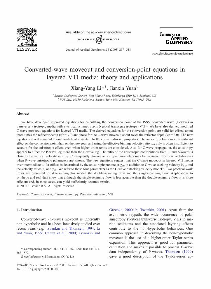
of ray-tracing. Fig. 2a shows the comparisons of the

anisotropic Eqs. (13), (18) and (19) with ray tracing,

and Fig. 2b shows the comparison of the isotropic

Eqs. (13), (18) and (22) with ray tracing. Note that the

difference between Fig. 2a and b lies in the calculation

of the coefficient c2. Fig. 2a uses the anisotropic Eq.

(19) and Fig. 2b uses the isotropic Eq. (22). For all

three reflectors, the conversion point error is less than

0.5% for x/z = 1.0 and less than 1.5% for x/z= 3.0

when using the anisotropic Eq. (19) (Fig. 2a). How-

ever, if the anisotropy parameters geff and feff are

ignored, the error increases to 5% for x/z = 1.0 and to

more than 10% for x/z= 3.0 (Fig. 2b).

3.4. Effects of geff and feff

For most earth models, one can expect that geff andfeff have the same sign. Thus, the residual term

[8(geffc0ceff + feff)] in Eq. (19) may often be of the

same order as the first term (c0ceff� 1). This confirms

Gaiser and Jackson’s (2000) numerical analysis that

compensating for ceff only, i.e., ignoring the term

[8(geffc0ceff + feff)] in Eq. (19) is not sufficient to

account for anisotropy. They also found that an

increase in e or a decrease in d increases the errors

in xC. This can be easily explained by Eq. (19) or Eq.

(23), since either an increase in e or a decrease in dgives rise to an increase in g or f, and hence increases

the errors in xC.

It is also worth noting that the residual term after

ceff compensation in Eq. (19) is determined by the

anisotropic parameters g and f, rather than by d and rdirectly. (As d does for P-wave, r measures the

relative difference between the S-wave stacking and

vertical velocity; Thomsen, 1986.) As shown in Sec-

Fig. 2. Accuracy of approximations for the three-layer model in

Table 1. (a) Results obtained from Eq. (19) that consider both ceffand the anisotropic residual term, and (b) results from Eq. (22) that

only considers ceff and ignores the residual anisotropic term. The

horizontal axis is the offset-to-depth ratio x/z, and the vertical axis is

the relative error of the conversion point xC calculated as

[xC(exact)� xC

(approx)]/x. The dotted line is from the first reflector, the

solid line from the second reflector and the dashed line from the

third reflector.


tion 4, C-wave moveout signature is also determined

by g and f.

4. Taylor-series based moveout equations

Tsvankin and Thomsen (1994) derived a generic

form of the C-wave moveout equation based on a

Taylor series expansion, but their expression for the

quadratic coefficient A4 is of a complicate form.

Thomsen (1999) and Cheret et al. (2000) presented

simplified forms. However, the expression for A4 in

Thomsen’s (1999) paper is less accurate and limited to

an offset-depth ratio of 1.0. The expression for A4 in

Cheret et al. (2000) contains a parameter called the

‘‘horizontal converted-wave velocity’’ (VCh), which is

not well defined and difficult to determine. Here, we

present an alternative and more accurate approach to

utilize the non-hyperbolic moveout equation of Tsvan-

kin and Thomsen (1994) for moveout analysis in

layered VTI media.

4.1. Generalized equations

The moveout for a C-wave ray tC, converted at the

bottom of the n-th layer and emerging at offset x (Fig.

1), can be written as (Tsvankin and Thomsen, 1994)

t2C ¼ t2C0 þx2

V 2C2

þ A4x4

1þ A5x2ð24Þ

where (see Appendix B)

A4 ¼ðc0ceff � 1Þ2 þ 8ð1þ c0Þðgeffc0c2eff � feff Þ


;

ð25Þ

and

A5 ¼A4

1=V 2Ph � 1=V 2

C2

: ð26Þ

VPh is the horizontal P-wave velocity.

4.2. The four-parameter moveout equation

Introduce a combined parameter veff,

veff ¼ geffc0c2eff � feff ; ð27Þ

which describes the total influence of the VTI and

layering on the C-wave moveout signature. Note that

for a single VTI layer, Eq. (27) reduces to

v ¼ gðc0 � 1Þc2eff : ð28Þ

substituting Eq. (27) into Eq. (25) gives

A4 ¼ � ðc0ceff � 1Þ2 þ 8ð1þ c0Þveff4t2C0V

4C2c0ð1þ ceff Þ2

: ð29Þ

Following Alkhalifah and Tsvankin’s (1955) em-

pirical relationship between VPh and geff, we suggest asimilar empirical relationship between VPh and veff,

VPh ¼ VP2

ffiffiffiffiffiffiffiffiffiffiffiffiffiffi1þ 2g

pcVP2

ffiffiffiffiffiffiffiffiffiffiffiffiffiffiffiffiffiffiffiffiffiffiffiffiffiffiffiffiffiffiffiffiffiffi1þ 2veff

ðc0 � 1Þc2eff:

sð30Þ

Fig. 3. Accuracy of the moveout approximations for the three-layer

model in Table 1. The residual moveout is calculated as DtC =

tC(exact)� tC

(approx), and tC(exact) is calculated by ray tracing. (a) Results

of the four-parameter Eqs. (24), (29) and (31), and (b) those of the

isotropic equations with geff = 0 and feff = 0 from Thomsen (1999).

The horizontal axis is the offset-to-depth ratio, and the vertical axis

is the residual moveout. The dotted line is from the first reflector,

the solid line from the second reflector and the dashed line from the

third reflector.

X.-Y. Li, J. Yuan / Journal of Applied

The above equation is strictly valid only for a single

VTI layer, but it is a good approximation for move-

out analysis in layered media. Substituting Eqs. (29)

and (30) into Eq. (26) and using Eq. (7) gives,

A5 ¼A4V

2C2ð1þ c0Þceff ðc0 � 1Þc2eff þ 2veff

� �ðc0 � 1Þc2eff ð1� c0ceff Þ � 2ð1þ c0Þceffveff

:

ð31Þ

Thus, the C-wave moveout, as described by Eqs. (24),

(29) and (31), is controlled by four parameters, VC2,

c0, ceff and veff. We refer to Eqs. (24), (29) and (31) as

the four parameter equations, which form the basis for

parameter estimation and moveout correction. Note

that the P-wave moveout signature is controlled only

by two parameters VP2 and geff.

4.3. Special cases

Here, for comparison, we consider the special cases

of a single isotropic layer and a single VTI layer,

which were studied by Thomsen (1999).

4.3.1. Single isotropic layer

In this case, ceff = c0, veff = 0 and Eqs. (29) and (31)

reduce to

A4 ¼�ðc0 � 1Þ2

4t2C0V4C2c0

; A5 ¼A4V

2C2c0

1� c0: ð32Þ

Eq. (32) differs from the original equation given in

Thomsen (1999) here referred to as A4*, which has the

following form,

A4* ¼ �ðc0 � 1Þ2

4t2C0V4C2ðc0 þ 1Þ ; A5 ¼

A4*V2C2c0

1� c0: ð33Þ

4.3.2. Single VTI layer

In this case, Eq. (29) reduces to

A4¼�1

t2C0V2C2ð1þ ceff Þ2

2gðc20 � 1Þ

c0c2eff þ

ðc22 � 1Þ2

4c0

" #:

ð34Þ

and has the same for as Eq. (31). Again note that Eq.

(34) differs from the original equation in Thomsen

(1999) in the isotropic term.

4.4. Accuracy and comparison

We first examine the accuracy of the four-param-

eter Eqs. (24), (29) and (31). We then compare the

accuracy of the isotropic Eqs. (32) and (33) since they

differ from each other. For the first task, we again use

the model in Table 1. The moveouts calculated by the

approximate equations are compared with those by

ray-tracing. Fig. 3a shows the output of Eqs. (24), (29)

and (31), and Fig. 3b shows the output of the isotropic

equations (letting veff = 0). The new approximations

are accurate up to the offset-to-depth ratio (x/z) of 2.0,

whilst the isotropic equations are only accurate to x/z

of 1.0.

To examine the accuracy of Eqs. (32) and (33), we

use the simple model of a single isotropic layer. The

results are shown in Fig. 4. For comparison, we also

enclose the results of the hyperbolic moveout equa-

Geophysics 54 (2003) 297–318 303

Fig. 4. Accuracy of moveout approximation for a single isotropic layer with VP= 2500 m/s, c0 = 2.5 and depth at 1000 m. The three

approximations are: squares—hyperbolic, crosses—Eq. (33) derived by Thomsen (1999) and circles—new Eq. (32). The residual moveout is

calculated as DtC = tC(exact)� tC

(approx), and tC(exact) is calculated by ray tracing.


tion. We can see that the hyperbolic moveout equation

is accurate up to x/z = 0.7, and the original Thomsen

equation is accurate to x/z = 1.0, whereas the new

equation is accurate up to x/z = 0.7. Note that, for

multilayer media, the new equations are more accurate

than for the single-layer case.

Table 2

Influence of P- and S-wave anisotropy on converted wave in single-

layered medium

Material xC—Eq. (19) tC—Eq. (25)

gc0ceff f= gceff2 gc0ceff

2 f= gceff2

Dog Creek shale 0.282 0.154 0.335 0.154

Pierre shale � 0.434 � 0.932 � 2.06 � 0.932

Taylor sandstone 0.248 0.113 0.214 0.113

5. Influence of anisotropy on converted-waves

VTI influences both the position of the conversion

point and converted-wave moveout. This influence

comes from two sources, the P-wave anisotropy

described by g or geff and the S-wave anisotropy

described by f or feff. One intriguing question is

whether the effects of anisotropy seen in the con-

verted-wave are mainly from the P-wave leg, the S-

wave leg or both. This has implications in parameter

estimation. For examples, if the converted-wave an-

isotropy is mainly from the P-wave leg, then we may

still not be able to recover all the necessary aniso-

tropic information even if both P-wave and converted-

wave are available. With the above analytical equa-

tions, it is possible to gain some insight into this

problem.

5.1. P-wave anisotropy vs. S-wave anisotropy

For simplicity, we consider the single-layer case.

We represent the anisotropic effects using the corres-

ponding terms in Eqs. (19) and (25) for P- and S-

waves, respectively. For example, for conversion-

point calculation, the corresponding term representing

the P-wave anisotropic effect is gc0ceff2 (Eq. (19)) and,

for moveout, the P-wave anisotropic term is gc0ceff2 . In

both cases, the S-wave anisotropic term is f = gceff2 .

Therefore, for anisotropic materials with ceff close to

1.0, the ratio of the anisotropic contributions from P-

and S-waves is close to c0. Table 2 lists these terms for

three materials, Dog Creek shale, Pierre shale and

Taylor sandstone. It can be seen that the P-wave

anisotropic term is about c0 times larger than that of

the S-wave in both conversion-point and moveout

calculations. The only exception is the calculation of

conversion point xC for Pierre shale, where the S-

wave anisotropic term is stronger. Note that Pierre

shale has a negative r, giving rise to a ceff larger thanc0, which is relatively rare in published measurements

(Thomsen, 1986).

In multilayered media, g and f are replaced by geffand feff. From their definitions in Eqs. (16) and (17),


both geff and feff are combinations of the layering

effect and interval anisotropy. However, as follows

from the definition of geff, the layering effect and

interval gi reinforce each other, and thus geff generallyincreases with depth, as shown in the three-layer

model in Table 1. In contrast, for feff, the layering

effect and interval fi have opposite signs, and thus

cause feff to decrease with depth (Table 1).

In summary, the P-wave anisotropic term appears

to be larger than the S-wave anisotropic term, partic-

ularly for moveout calculation. From the cases we

examined, the ratio of P- to S-wave anisotropic terms

is close to the vertical velocity ratio c0. Thus, it may

be possible to recover S-wave anisotropic information

from converted-wave data.

5.2. Conversion-point vs. moveout

As shown Fig. 2b, if anisotropy is ignored in the

calculation of the conversion point (letting geff = 0 and

feff = 0), the isotropic Eq. (22) is only accurate for

offsets up to half the reflector depth (x/z= 0.5). In

comparison, if anisotropy is ignored in the moveout

calculation, the isotropic equation is still accurate for

offsets up to the reflector depth (x/z= 1.0), as shown

in Fig. 3b. This shows that VTI has a stronger

influence on the conversion point than on moveout.

This can also be explained from the analytical equa-

tions. As shown in Eq. (19), P-wave anisotropy (geff)and S-wave anisotropy (feff) reinforce each other in

determining the conversion point, whilst they have

opposite signs in Eq. (25). This further increases the

anisotropic influence on the calculation of the con-

version point, which may lead to mis-positioning of

reservoir formations.

6. Implications for parameter estimation

The above expressions for converted-wave kine-

matic include three kinds of parameters: medium

Fig. 5. Sensitivity analysis for a single VTI layer of Dog Creek shale

(VP0 = 1875 m/s, VS0 = 826 m/s, e= 0.225 and d= 0.1) at depth

z = 1000 m. (a) Synthetic gather. (b) Double-scanning for c0 and ceffby fixing VC2 (1540 m/s) and veff (0.187). (c) Double-scanning for

VC2 and veff by fixing c0 (2.270) and ceff (1.191). The dots indicatemodel results.


parameters, conversion-point attributes and moveout

attributes. The medium parameters may include the P-

and S-wave stacking velocities VP2 and VS2, vertical

velocity ratio c0, and P- and S-wave anisotropic

parameters geff and feff. Note that the four generic

Thomsen parameters are also medium parameters

which are required for depth processing. The C-wave

moveout attributes may include VC2 and veff, whilstceff is a conversion-point attribute. With this kind of

parameterization, the issue is how to estimate the

stacking velocity model VC2, c0, ceff and veff usingthe new equations. Here, we examine the sensitivity to

the parameters, and investigate the viability of the

double-scanning procedure for parameter estimation.

6.1. Sensitivity analysis of velocity ratios c0 and ceff

In general, the C-wave moveout is not sensitive to

variations of c0 and ceff (Li and Yuan, 2001). Fig. 5a

and b illustrate whether or not the two velocity ratios

can be resolved by semblance analysis with sufficient

resolution and accuracy, where we assume known VC2

and veff and directly invert for c0 and ceff. Syntheticmodelling (Fig. 5a) is generated by ray tracing for the

Dog Creek shale, and the depth of reflector is 1000 m,

maximum offset is 3000 m, and a 30 Hz Ricker’s

wavelet is used. Eq. (24) is used for inversion, where

the exact VC2 and veff values are used as inputs. The

traces are stacked for semblance analysis as shown in

Fig. 5b. The resolutions of semblance analysis for

Fig. 6. Error propagation from estimated VC2 to ceff. Three curves indicate(circles), respectively.

both c0 and ceff are poor. Tests have also been carried

out for other materials (Pierre shale and Taylor sand-

stone; Yuan, 2002) and all materials studied show

poor resolution when determining c0 and ceff fromsemblance analysis. These results indicate that c0 andceff may be difficult, if not impossible, to obtain from

C-wave moveout inversion. On the other hand, if c0and ceff are fixed, double scanning for VC2 and veffshows good resolution and correct results (Fig. 5c).

6.2. Estimating c0 and ceff

The previous results suggest that c0 and ceff can notbe determined from C-wave reaction moveout, and

that correlation of P- and C-wave sections is likely the

only means to obtain a reliable c0 in the absence of

other independent information. The next question is

how to estimate ceff?First, from the conversion-point Eqs. (13), (18) and

(19), one can see that ceff is separated from other

parameters in the first order term. Thus, ceff can be

reliably determined from the conversion-point signa-

ture provided the signature can be estimated from the

data. This forms the basis of the CCP scanning

technique (Bagaini et al., 1999). Unfortunately, the

conversion-point signature can only be estimated in

the presence of certain geological features, such as the

apex of an anticline, a fault or a dipping layer.

Secondly, if VP2, VC2 and c0 are known, ceff may be

determined from Eq. (6). However, error propagation

different velocity ratios VP/VS: 2.0 (triangles), 2.5 (squares) and 3.0


is known to be a problem for this approach. Normally,

VP2 can be determined rather precisely from P-wave

data when signal-to-noise ratio is reasonable, whereas

errors are often associated with VC2, and will propa-

gate into ceff through Eq. (6).

Fig. 6 shows the error propagation from VC2 to cefffor different velocity ratios. A 3% error in VC2 will

result in 15–20% errors in ceff when the average

velocity ratio varies from 2.0 to 3.0. Thus, the use

of Eq. (6) for estimating ceff requires accurate deter-

mination of VC2 with errors less than 2%, assuming a

10% error margin in ceff.

Fig. 7. Semblance analysis for VC2 and veff with a priori information about ccircles are model values of VC2 and veff. (a) Synthetic seismogram from ray

reflector and (d) third reflector.

6.3. Double-scanning in layered VTI media

Here we use the three-layer model in Table 1 to

demonstrate the viability of the double-scanning pro-

cedure in layered media. We assume that c0 was

obtained by correlating P- and C-wave stacked sec-

tions, and ceff was found from Eq. (6), where the P-

wave moveout velocity VP2 can be determined from

P-wave data. Fig. 7a is a synthetic gather calculated

by ray tracing for the three-layer model in Table 1.

Fig. 7b–d shows the results of semblance analyses for

VC2 and veff, using ceff and c0 as a priori information.

0 and ceff for a given tC0, using the three-term moveout Eq. (24). The

tracing and semblance analysis for the (b) first reflector, (c) second


The offset range used for semblance analysis is

limited to an offset-to-depth ratio of 2.0. The circles

are the exact values of VC2 and veff. The semblance

spectra show high resolution and good inversion

results for VC2 and veff.Note that it may be easy to confuse the issues

of moveout correction and parameter estimation.

Moveout correction itself can be accomplished using

the generic form of Tsvankin and Thomsen (1994)

with the coefficients determined by semblance anal-

ysis. In contrast, parameter estimation requires accu-

rate analytical expressions for the relevant moveout

coefficients, and this is the main purpose of this

paper.

6.4. Error analysis

The above analysis shows that the modified move-

out Eqs. (24), (29) and (31) allow the use of existing P-

wave semblance procedures, as developed by Grechka

and Tsvankin (1988), for C-wave moveout analysis

and parameter estimation. Grechka and Tsvankin

(1988) also gave a detailed account of the effects

of correlated travel-time errors on non-hyperbolic

moveout analysis. They showed that random travel-

time errors have very little influence on the results

of semblance analysis. In contrast, correlated travel-

time errors can have a significant effect, although they

may not affect the resolution of the semblance analy-

sis. These findings are expected to hold for C-wave

moveout analysis as well.

7. Single-scanning for estimating VC2 and ceff

The double-scanning procedure may be robust, but

may also be time-consuming. Thus, it is worth to

investigate the use of single-scanning procedure for

parameter estimation. For this, the accuracy of VC2 is

essential. VC2 is the short-spread NMO stacking

velocity, but it often cannot be determined accurately

using conventional hyperbolic procedures.

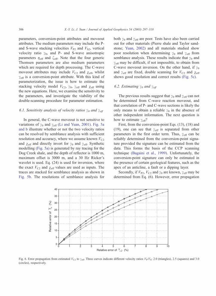
7.1. Single-scanning for VC2

Here, we introduce a simple single-scanning pro-

cedure over the intermediate offsets (offset-depth ratio

up to x/z= 1.5) for determining VC2 accurately. The

procedure utilizes a background c to quantify the non-

hyperbolic moveout over the intermediate offsets. The

C-wave moveout over intermediate offsets up to x/

z = 1.5 may be expressed as, with a background

velocity ratio c (Yuan, 2002),

t2C ¼ t2C0 þx2

V 2C2

� ðc � 1Þ2

cV 2C2

x4

4t2C0V2C2 þ ðc � 1Þx2 :

ð35Þ

Thus, if a background velocity ratio c is given, we

may use Eq. (35) for velocity analysis. We test this

idea using the synthetic data in Fig. 7a, and the single-

scanning results of VC2 are shown in Fig. 8. The errors

in hyperbolic analysis are about 3% over offsets up to

x/z = 1.0 (Fig. 8a), whilst those in the non-hyperbolic

analysis are less than 1% over offsets up to x/z = 1.5

(Fig. 8b and c).

To check the influence of the background velocity

ratio on velocity analysis, a velocity ratio of 2.0 is

used in Fig. 8b, whilst a velocity ratio of 3.0 is used in

Fig. 8c. Comparing Fig. 8b with Fig. 8c shows that

20% change in velocity ratio does not affect VC2

scanning results very much. The insensitivity of C-

wave moveout signature to the velocity ratios over

intermediate offsets means that for velocity analysis

purposes, detailed knowledge about the velocity ratio

is not necessary. The differences between c0 and ceffcan also be ignored. This justifies the use of a

homogeneous and isotropic Eq. (35) for non-hyper-

bolic moveout analysis over intermediate offsets.

7.2. Single-scanning for veff

The previous section shows that it is possible to

determine VC2 accurately from intermediate offsets

using non-hyperbolic velocity analysis. Thus, with

VC2, c0 and ceff all determined, it may be possible to

determine veff by a single-scanning technique from the

far offset C-wave data affected by veff. Here, we use

the three-layer model in Figs. 7a and 8 to test this

idea. Fig. 9 shows the results with good resolution and

accuracy. However, this single-scanning technique is

very sensitive to the accuracy of VC2. A 2% pertur-

bation in VC2 gives about 15% changes in veff. Notehere the input VC2 is 2% higher than the exact values,

which gives the veff curve a constant shift toward the

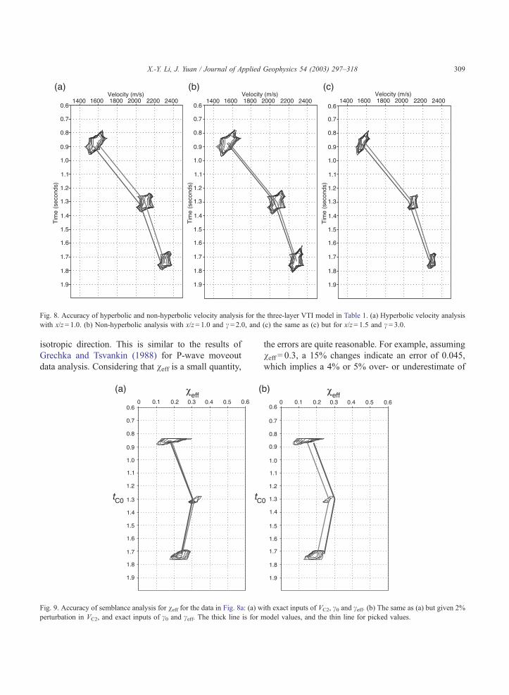
Fig. 8. Accuracy of hyperbolic and non-hyperbolic velocity analysis for the three-layer VTI model in Table 1. (a) Hyperbolic velocity analysis

with x/z = 1.0. (b) Non-hyperbolic analysis with x/z = 1.0 and c = 2.0, and (c) the same as (c) but for x/z = 1.5 and c= 3.0.


isotropic direction. This is similar to the results of

Grechka and Tsvankin (1988) for P-wave moveout

data analysis. Considering that veff is a small quantity,

Fig. 9. Accuracy of semblance analysis for veff for the data in Fig. 8a: (a) w

perturbation in VC2, and exact inputs of c0 and ceff. The thick line is for m

the errors are quite reasonable. For example, assuming

veff = 0.3, a 15% changes indicate an error of 0.045,

which implies a 4% or 5% over- or underestimate of

ith exact inputs of VC2, c0 and ceff. (b) The same as (a) but given 2%

odel values, and the thin line for picked values.


the anisotropy. Still, due to trade-offs between VC2

and veff, the single-scanning procedures have to be

used carefully.

8. Work flows for anisotropic velocity analysis

From the above theoretical and numerical analyses,

two possible work flows can be suggested to deter-

mine the stacking velocity model (VC2, c0, ceff andveff) using 4C seismic data: a double-scanning work

flow and a single-scanning work flow.

8.1. The double-scanning work flow

In the numerical analysis, we used c0 and ceff asinput parameters for the double-scanning algorithm.

In real data processing, it may be more convenient to

use VP2 to replace ceff as the input parameter. During

the scanning process, for each given set of VP2, VC2

and c0, the corresponding ceff can be calculated using

Eq. (6). This increases the computation of double

scanning, but simplifies the work flow and reduces

the number of iterations. (The flow involves one

iteration for VC2 due to the requirement for correlation

to obtain c0.) With this in mind, the work flow can be

designed as follows.

The first step is to process the P-wave data and

build the P-wave velocity model VP2. This is inde-

pendent of the C-wave data. Standard methods may be

used to obtain the best imaging and the velocity

model.

The second step is to obtain c0 through an initial

processing of the C-wave data and a coarse correlation

with the P-wave data. The main purpose of the C-

wave processing is to obtain a brute stack for corre-

lation with the P-wave section. The key information to

preserve during processing is the time tC0. Thus,

standard hyperbolic processing can be used and the

C-wave data may even be processed in the CDP

domain. Care should be taken to limit the data to

the short offsets up to x/z = 1.0. The third step is to

determine VC2 and veff by the double-scanning proce-

dure on selected horizons using VP2 and c0 as input

parameters. The final step is to determine ceff usingEq. (6) from VP2 and VC2. Note that here VC2 is the

double scanning result. During the initial processing

of the C-wave data, an initial estimate of VC2* is also

obtained from hyperbolic analysis; this VC2* should be

ignored.

8.2. The single-scanning work flow

This flow also has four steps. The first step is the

P-wave processing and is the same as that in the

double scanning work flow.

The second step is to obtain accurate estimates of

VC2 by non-hyperbolic velocity analysis using Eq.

(35). The C-wave data is processed in the ACCP

Asymptotic Common Conversion Point domain with

a background c. After ACCP binning, non-hyperbolic

velocity analysis with the same c is employed to

determine VC2 and to generate a C-wave stacked

section. The data have to be limited to the intermedi-

ate offsets up to x/z= 1.5. The third step is to estimate

c0 and ceff. As before, c0 is estimated by a coarse

correlation of the P- and C-wave stacked sections, and

ceff is obtained from Eq. (6) using VP2, VC2 and c0 asinputs.

Once VC2, c0 and ceff are determined, the final

step is to obtain veff by single-scanning semblance

analysis as shown in Fig. 9 over the entire offsets

up to x/z = 3.0.

This work flow is more efficient in real data

processing. However, the single-scanning results of

veff has an error margin of 15–20% depending on the

accuracy of VC2, as shown in the synthetic test (Fig.

9), and this trade-off may invalidate the single-scan-

ning procedure.

9. Field data example

The above work flows have been applied to several

4C datasets from the North Sea including Guillemot,

Alba and Valhall; here, we use the Guillemot 4C data

(courtesy of Shell Expro). Details of acquisition

geometry of this dataset were documented in Yuan

et al. (1998) and standard P- and C-wave wave

processing can also be found in Yuan et al. (1998)

and Li and Yuan (1999).

We select the gathers at CCP (or CDP) 1100 to

illustrate anisotropic velocity analysis. In this con-

text, CCP and CDP are co-located. Fig. 10 shows

the P- and C-wave data at location CCP 1100. A

background c of 2.5 was used to obtain the CCP

Fig. 10. (a) P-wave CDP gather at CDP 1100 of the Guillemot data and (b) the corresponding C-wave gather at CCP 1100. CDPs and CCPs are

co-located. The solid lines mark some horizons correlated by Yuan et al. (1998).


gather. Some correlated horizons based on previous

work (e.g., Yuan et al., 1998; Li and Yuan, 1999)

are marked on the data. The overall quality of this

dataset is excellent, and the processing of both P-

and C-wave is straightforward. The estimated P-

wave stacking velocity VP2 and vertical velocity

ratio c0 at CDP or CCP location 1100 (both

obtained by conventional processing) are listed in

Table 3 for the three correlated events in Fig. 10.

Next, using these as a priori information, we ex-

amine the sensitivity of double-scanning, the accu-

racy of non-hyperbolic velocity analysis, and the

effectiveness of single-scanning.

Table 3

VC2, ceff and veff obtained from the double-scanning work flow (Fig. 11)

analysis for VC2 (Fig. 12) and single scanning for veff (Fig. 14)

No. tC0 (ms) tP0 (ms) VP2 (ms) c0 Doub

VC2 (

1 1531 707 1920 3.33 1130

2 2064 980 2000 3.21 1165

3 2574 1243 2047 3.14 1235

9.1. Double scanning for VC2 and veff

The three correlated events at tC0 = 1520, 2050 and

2570 ms (Fig. 10) are selected to illustrate the double-

scanning processing. The input parameters are VP2

and c0 and are listed in Table 3. Good resolution in

VC2 and veff is obtained, and values picked from Fig.

11a–c are listed in Table 3. The average veff is about0.22, indicating a significant amount of converted-

wave anisotropy.

To test the sensitivity of double-scanning to errors

in the input parameters, we add 10% errors to the

input c0, and the corresponding double scanning

and single-scanning work flow including non-hyperbolic velocity

le scanning Single scanning (non-hyperbolic)

m/s) ceff veff VC2 (m/s) ceff veff

2.00 0.16 1120 2.10 0.23

2.33 0.26 1190 2.04 0.21

1.97 0.27 1240 1.93 0.28

Fig. 11. Double-scanning analysis for VC2 and ceff using a priori information for VP2 and c0 for the data in Fig. 10b. VP2 and c0 are listed in Table 3.Events at (a) tC0 = 1520 ms, (b) tC0 = 2050 ms and (c) tC0 = 2570 ms. (d), (e) and (f) are the same as (a), (b) and (c), but there are 10% errors added

to the corresponding c0.


results are shown in Fig. 11d–f. The errors in c0 havealmost no effect on VC2, but there are about 15%

differences in the values of veff.

9.2. Non-hyperbolic velocity analysis for VC2

Eq. (35) has been used to perform non-hyperbolic

velocity analysis with the same background c= 2.5 as

ACCP binning. The offsets are limited to the inter-

mediate range up to x/z = 1.5 in order to determine

VC2. Fig. 12a shows the semblance spectra for the

CCP gather in Fig. 10b. Fig. 12b shows the

corresponding hyperbolic spectra for comparison.

The two lines show a possible picking error of 2%.

The quality of the spectra obtained by non-hyperbolic

velocity analysis is substantially improved in terms of

the signal-to-noise ratio. There are 5–7% differences

between the non-hyperbolic and hyperbolic results

(Fig. 12). The difference in velocities is substantial

and is due to the significant non-hyperbolic moveout

enhanced by the presence of anisotropy.

9.3. Verifications and comparisons

There are 1–2% differences between the VC2

from double scanning and those from non-hyperbol-

ic velocity analysis (Table 3). They both differ from

the hyperbolic VC2* significantly. To examine the

accuracy of these velocities, we use them to perform

moveout correction by Eq. (24), and the results are

shown in Fig. 13. Most events are substantially

under-corrected when the hyperbolic velocities VC2*

are used for moveout correction, confirming that VC2*

is too high (Fig. 13b). In contrast, most of the

events are properly aligned when using the non-

hyperbolic velocity (Fig. 13a), except for the events

at tC0 = 1.6 s and tC0 = 2.1 s, which are slightly over-

corrected. In Fig. 13a and b, veff is set to zero. Note

that those events at tC0 = 1.6 s and tC0 = 1.6 s can

also be aligned with corresponding veff values of

0.16 and 0.26 (Fig. 13c). This shows that the veffhas accurately captured the anisotropic effects in the

data.

Fig. 12. Comparison of (a) non-hyperbolic with (b) hyperbolic velocity analyses for the intermediate offsets up to x/z = 1.5. The lines show a

possible picking error of 2%.

Fig. 13. Comparison of C-wave moveout correction using different values of VC2. ceff and veff with c0 fixed as in Table 3: (a) veff = 0 and VC2 and

ceff from the non-hyperbolic velocity analysis in Fig. 12a; (b) the same as in a but VC2 and ceff from the hyperbolic velocity analysis in Fig. 12b;

(c) the same as in (a) but veff from the double-scanning analysis in Fig. 11.


plied Geophysics 54 (2003) 297–318

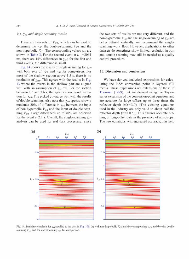
9.4. ceff and single-scanning results

There are two sets of VC2, which can be used to

determine the ceff: the double-scanning VC2 and the

non-hyperbolic VC2. The corresponding values ceff areshown in Table 3. For the second event at tC0 = 2064

ms, there are 15% differences in ceff; for the first and

third events, the difference is small.

Fig. 14 shows the results of single-scanning for veffwith both sets of VC2 and ceff for comparison. For

most of the shallow section above 1.5 s, there is no

resolution of veff. This agrees with the results in Fig.

13 where the events in the shallow part are aligned

well with an assumption of veff = 0. For the section

between 1.5 and 2.6 s, the spectra show good resolu-

tion for veff. The picked veff agree well with the resultsof double scanning. Also note that veff spectra show a

moderate 20% of difference in veff between the input

of non-hyperbolic VC2 and the input of double scan-

ning VC2. Large differences up to 40% are observed

for the event at 2.1 s. Overall, the single-scanning veffanalysis can be used for real data processing. Since

X.-Y. Li, J. Yuan / Journal of Ap314

Fig. 14. Semblance analysis for veff applied to the data in Fig. 10b: (a) with

scanning VC2 and the corresponding ceff for comparison.

the two sets of results are not very different, and the

non-hyperbolic VC2 and the single-scanning of veff arebetter defined vertically, we recommend the single-

scanning work flow. However, applications to other

datasets do sometimes show limited resolution in veff,and double-scanning may still be needed as a quality

control procedure.

10. Discussion and conclusions

We have derived analytical expressions for calcu-

lating the P-SV conversion point in layered VTI

media. These expressions are extensions of those in

Thomsen (1999), but are derived using the Taylor-

series expansion of the conversion-point equation, and

are accurate for large offsets up to three times the

reflector depth (x/z = 3.0). [The existing equations

used in the industry are only valid to about half the

reflector depth (x/z= 0.5).] This ensures accurate bin-

ning of long-offset data in the presence of anisotropy.

The new equations, with increased accuracy, may help

non-hyperbolic VC2 and the corresponding ceff, and (b) with double


to estimate anisotropy at locations with distinct geo-

logical features, such as fault points (Yuan and Li,

2002).

We have presented modified equations of Tsvankin

and Thomsen (1994) for calculating converted-wave

travel-times in layered VTI media in order to utilize

the existing semblance analysis procedures for param-

eter estimation. These equations are accurate up to

offsets twice the reflector depth (x/z = 2.0), as com-

pared to just x/z = 1.0 of those modified equations in

Thomsen (1999). The new equation uses four param-

eters to describe the C-wave moveout: the converted-

wave stacking velocity VC2, vertical velocity ratio c0,effective velocity ratio ceff and a new anisotropic

parameter veff.We have also discussed the application of these

equations for determining the C-wave stacking veloc-

ity model described by VC2, c0, ceff and veff, and

demonstrated the application using both synthetic and

real data. With a priori knowledge of the vertical and

effective velocity ratios c0 and ceff, the C-wave stack-ing velocity VC2 and the anisotropic parameter veffmay be estimated from far-offset C-wave data using

either a double-scanning or a single-scanning proce-

dure. Real data applications show that the double-

scanning is robust but time-consuming. The single-

scanning flow with non-hyperbolic velocity analysis

for VC2 may provide an alternative. The non-hyper-

bolic velocity analysis has a similar accuracy to that of

the double-scanning analysis, and veff obtained from

single-scanning semblance analysis agrees with the

double scanning results in most cases. However, care

should be taken with the single-scanning procedure

due to the trade-offs between parameters.

We conclude that the newly derived expressions

have captured the conversion-point and moveout

signatures in terms of measurable moveout attributes

for mid-to-long offset data. An anisotropic parameter

veff is introduced to quantify the anisotropic effects on

the C-wave reflaction moveout, and another coefficient

feff is introduced to quantify the anisotropic effects

in the S-wave leg of a C-wave ray. In a single-layered

VTI medium, veff = v = c0ceff2 g� f=(c0� 1)ceff

2 g, andfeff = f = ceff

2 g. The derived equations enable the use

of conventional procedures such as semblance anal-

ysis and Dix-type model building to implement

anisotropic processing, and make anisotropic pro-

cessing affordable.

Acknowledgements

We thank Leon Thomsen for useful discussion. We

thank Shell Expro for providing the Guillemot data

and for permission to show the data. The data was

original provided to the University of Edinburgh

industry-sponsored project Processing of four-compo-

nent Sea Floor Seismic Data (BP, DTI, Elf, Mobil,

PGS, Shell and Western Geophysical). We thank

Floris Strijbos and Professor Anton Ziolkowski for

agreeing to share the data with the Edinburgh

Anisotropy Project (EAP). This work is funded by

the EAP of the British Geological Survey (BGS) and

is published with the approval of the Executive

Director of the BGS and the EAP sponsors: Agip,

BG, BP, ChevronTexaco, CNPC, ConocoPhillips,

DTI/RIPED-LangFang, KerrMcGee, Landmark, Mar-

athon, Norsk Hydro, PGS, Schlumberger, Texaco,

TotalFinaElf, Veritas DGC.

Appendix A. Derivation of conversion-point

equation in layered anisotropic media

Consider a horizontally layered medium, as shown

in Fig. 1, with each layer being homogeneous and

transversely isotropic with a vertical symmetry axis

(VTI). vPi, wPi are the interval P-wave phase and

group velocities, vSi and wSi are their S-wave counter-

parts, and Dzi is the thickness of the i-th layer. hPi andhSi are the angles between the group velocity vectors

and the vertical axis. xP is the conversion point offset

from the source for the P-wave path, and xS is the

corresponding offset to the receiver for the shear wave

path. Note that in this context, we have xC = xP.

The total offset of ray path x is

x ¼ xP þ xS; ðA� 1Þwhere

xP ¼Xni¼1

DxPi ¼ pXni¼1

UPiDtPi;

xS ¼Xni¼1

DxSi ¼ pXni¼1

USiDtSi; Ui ¼w1i

p:

ðA� 2ÞHere, p is the horizontal component of slowness

vector (the ray parameter, dt/dx for the ray emerg-


ing at offset x, Dti is the oblique one-way travel-

time in the i-th layer, w1 is the horizontal compo-

nent of the group velocity vector. The subscripts

‘‘P’’ and ‘‘S’’ indicate terms related with P- or S-

wave paths.

Because xP is the odd function of x, Taylor series

expansion of the conversion point offset xP at total

offset x can be written as

xP ¼ limx!0

Xlk¼0

c2kx2kþ1 ¼ lim

p!0

Xlk¼0

c2kx2kþ1; ðA� 3Þ

where

c2k ¼1

ð2k þ 1Þ!d2kþ1xp

dx2kþ1:

A.1. Deriving Eq. (14) for c0

When k = 0,

c0 ¼ limp!0

dxp

dx¼ lim

p!0

dxp

dp

dp

dx: ðA� 4Þ

From Eqs. (A-1) and (A-2),

dxp

dp

dp

dx

¼

Xni¼1

UPiDtPi þ pd

dp

Xni¼1

UPiUPiDtPi

!

Xni¼1

UPiDtPi þ pd

dp

Xni¼1

UPiDtPi

!þXni¼1

USiDtSiþpd

dp

Xni¼1

USiDtSi

! ;

ðA� 5Þ

where

pd

dp

Xni¼1

UPiDtPi

!¼ pXni¼1

dUPi

dpDtPiþp2

Xni¼1

U 2PiDtPi;

ðA� 6Þ

pd

dp

Xni¼1

USiDtSi

!¼ pXni¼1

dUSi

dpDtSiþp2

Xni¼1

U 2SiDtSi:

ðA� 7Þ

For a VTI medium, Tsvankin and Thomsen (1994)

obtained

limp!0

UPi ¼ v2P2i ¼ v2P0ið1þ 2diÞ; ðA� 8Þ

limp!0

USi ¼ v2S2i ¼ v2S2ið1þ 2riÞ; ðA� 9Þ

limp!0

1

p

dUPi

dp¼ lim

p!0

d2UPi

dp2

¼ 8v4P0iðei � diÞ 1þ 2di

1� v2S0iv2P0i

0BBB@

1CCCA;

ðA� 10Þ

and

limp!0

1

p

dUSi

dp¼ lim

p!0

d2USi

dp2¼ �8v4S0iri 1þ 2di

1� v2S0iv2P0i

0BBB@

1CCCA:

ðA� 11Þ

Substituting Eqs. (A-8)–(A-11) into Eq. (A-4) and

taking the limit for the ray parameter p! 0, we get

Eq. (14).

A.2. Deriving Eq. (15) for c2

When k = 1,

c2 ¼1

6limp!0

d3xP

dx3:

By differentiating Eq. (A-5) with regard to p, after

some tedious algebraic manipulation, one can get

d3xP

dx3¼ d

dp

d

dp

dxP

dp

dp

dx

� �dp

dx

� �dp

dx

¼ðePþ pfPþeSþ pfSÞ

�3ðeSgP� ePgSÞþ p d

dpðeSgP� ePgSÞþ d

dpðp2ðfSgP� fPgSÞÞ

�ðeP þ pfP þ eS þ pfSÞ5

� 3ð2fP þ pgP þ 2fS þ pgSÞð2ðeS fP � ePfSÞ þ pðeSgP � ePgSÞ þ p2ðfSgP � fPgSÞÞðeP þ pfP þ eS þ pfSÞ5

ðA� 12Þ


where

e ¼Xni¼0

UiDti;

f ¼ de

dp¼ d

dp

Xni¼0

UiDti ¼Xni¼0

dUi

dpDti þ p

Xni¼0

U 2i Dti;

and

g ¼ df

dp¼Xni¼0

U2i Dti þ

Xni¼0

d2Ui

dp2Dti

þ3pX

Ui

dUi

dpDti þ p2

XU 3

i Dti:

From Eqs. (A-8)–(A-11), by taking the limit of p! 0,

we get

limp!0

eP ¼Xni¼0

v2P2iDtP0i ¼ V 2P2tP0; ðA� 13Þ

limp!0

eS ¼Xni¼0

v2S2iDtS0i ¼ V 2S2tS0; ðA� 14Þ

limp!0

fP ¼ limp!0

fS ¼ 0; ðA� 15Þ

limp!0

gP ¼ limp!0

Xni¼0

U2PiDtPi þ lim

p!0

Xni¼0

d2UPi

dp2DtPi

¼Xni¼0

v4P2iDtP0i þXni¼0

8v4P0iðei � diÞ

� 1þ 2di

1� v2S0iv2P0i

0B@

1CADtP0i; ðA� 16Þ

and

limp!0

gS ¼ limp!0

Xni¼0

U2SiDtSi þ lim

p!0

Xni¼0

d2USi

dp2DtSi

¼Xni¼0

v4S2iDtS0i �Xni¼0

8v4S0iri

� 1þ 2di

1� v2S0iv2P0i

0B@

1CADtS0i: ðA� 17Þ

Substituting Eqs. (A-13)–(A-17) into Eq. (A-12), the

c2 term of Taylor series expansion of conversion point

in layered VTI media becomes

c2 ¼1

6limp!0

d3xP

dx3¼ lim

p!0

ðeSgP � ePgSÞ2ðeP þ eSÞ4

¼ 1

2

V 2S2tS0

Xni¼0

DtP0iv4P0i ð1þ 2diÞ2 þ 8ðei � diÞ 1þ 2di

1� v2S0iv2P0i

0BBB@

1CCCA

0BBB@

1CCCA

0BBB@

1CCCA

ðV 2Pn2tP0 þ V 2

Sn2tS0Þ4

� 1

2

�V 2P2tP0

Xni¼0

DtS0iV4S0i ð1þ 2riÞ2 � 8ri 1þ 2di

1� v2S0iv2P0i

0BBB@

1CCCA

0BBB@

1CCCA

0BBB@

1CCCA

ðV 2P2tP0 þ V 2

S2tS0Þ4

:

ðA� 18Þ

Eqs. (9) and (10) in combination with Eq. (A-18)

gives Eq. (15).

Appendix B. Derivation of the C-wave moveout

equations in layered VTI media

The C-wave reaction moveout equation for lay-

ered VTI has the form (Tsvankin and Thomsen,

1994):

t2C ¼ t2C0 þx2

V 2C2

þ A4x4

1þ A5x2; ðB� 1Þ

where

A4 ¼tC0V

4C2 �

Xni¼1

ðHPi þ v4P2iÞDtP0i þXni¼0

ðHSi þ v4S2iÞDtS0i

!

4t3C0V8C2

;

ðB� 2Þ

HPi ¼ 8v4P0iðei � diÞ 1þ 2di1� 1=c20i

� �; ðB� 3Þ

and

HSi ¼ �8v4S0iri 1þ 2di1� 1=c20i

� �: ðB� 4Þ


Using the parameters gi and fi defined by Eqs. (9)

and (10), we obtain

HPi ¼ 8v4P2igi; ðB� 5Þ

and

HSi ¼ �8v4S2ifi: ðB� 6Þ

Inserting the definitions of geff and feff from Eqs.

(16) and (17) gives

Xni¼1

ðHPi þ v4P2iÞDtP0i ¼ ð1þ 8geff ÞtP0V 4P2; ðB� 7Þ

and

Xni¼1

ðHSi þ v4S2iÞDtS0i ¼ ð1� 8feff ÞtS0V 4S2: ðB� 8Þ

Substituting Eqs. (B-7) and (B-8) into Eq. (B-2)

gives

A4 ¼tC0V

4C2�ðð1þ8geff ÞtP0V 4

P2þð1�8feff ÞtS0V 4S2Þ

4t3C0V8C2

:

ðB� 9Þ

Replacing VP2 and VS2 with VC2, and tP0 and tS0 with

tC0, we obtain

A4 ¼ðc0ceff � 1Þ2 þ 8ð1þ c0Þðgeffc0c2eff � feff Þ


:

ðB� 10Þ

References

Alkhalifah, T., Tsvankin, I., 1995. Velocity analysis for transversely

isotropic media. Geophysics 60, 1550–1566.

Bagaini, C., Bale, R., Caprioli, P., Ronen, S., 1999. Converted wave

binning analysis: in search of c. 69th Internat. Mtg., Soc. Explor.

Geophys. Expanded., pp. 703–706.

Cheret, T., Bale, R., Leaney, S., 2000. Parameterization of polar

anisotropic moveout for converted waves. 70th Annual Internat.

Mtg., Soc. Expl. Expanded Abstracts., pp. 1181–1184.

Gaiser, J.E., Jackson, A.R., 2000. Accuracy and limitations of

PS-wave converted-point computations: how effective is ceff?70th Annual Internat. Mtg., Soc. Expl. Expanded Abstracts.,

pp. 1138–1141.

Grechka, V., Tsvankin, I., 1988. Feasibility of nonhyperbolic move-

out inversion in transversely isotropic media. Geophysics 63,

957–969.

Li, X.-Y., Yuan, J., 1999. Converted-wave moveout and parameter

estimation for transverse isotropy. 61st EAGE Conference, Ex-

panded Abstract, vol. I, pp. 4–35.

Li, X.-Y., Yuan, J., 2001. Converted-wave imaging in inhomoge-

neous, anisotropic media: Part I. Parameter estimation. 63rd

EAGE Conference, Expanded Abstract, vol. I, p. 109.

Tessmer, G., Behle, A., 1988. Common reaction point data-stacking

technique for convertedwaves. Geophys. Prospect. 36, 671–688.

Thomsen, L., 1986. Weak elastic anisotropy. Geophysics 51,

1954–1966.

Thomsen, L., 1999. Converted-wave reflection seismology over

inhomogeneous, anisotropic media. Geophysics 64, 678–690.

Tsvankin, I., 2001. Seismic Signatures and Analysis of Reaction

Data in Anisotropic Media. Elsevier.

Tsvankin, I., Grechka, V., 2000a. Dip moveout of converted waves

and parameter estimation in transversely isotropic media. Geo-

phys. Prospect. 48, 257–292.

Tsvankin, I., Grechka, V., 2000b. Two approaches to anisotropic

velocity analysis of converted waves. 70th Annual Internat.

Mtg., Soc. Expl. Expanded Abstracts., pp. 1193–1196.

Tsvankin, I., Thomsen, L., 1994. Nonhyperbolic reflection moveout

in anisotropic media. Geophysics 59, 1290–1304.

Yuan, J., 2002. Analysis of four-component seaoor seismic data for

seismic anisotropy. PhD thesis, The University of Edinburgh.

Yuan, J., Li, X.-Y., 2002. C-wave anisotropic parameter estimation

from conversion point. 64th EAGE Conference, Expanded Ab-

stract, vol. II, p. 253.

Yuan, J., Li, X.-Y., Ziolkowski, A., Strijbos, F., 1998. Processing

4C sea-floor seismic data: a case example from the North

Sea. 68th Ann. Internat. SEG Mtg., Expanded Abstracts.,

pp. 714–717.

Converted-wave moveout and conversion-point equations … · Converted-wave moveout and...

Documents

Transcript of Converted-wave moveout and conversion-point equations … · Converted-wave moveout and...