Louisiana State UniversityLSU Digital Commons

LSU Historical Dissertations and Theses Graduate School

1970

Convergence of the Finite Element Method.Nasrollah TabandehLouisiana State University and Agricultural & Mechanical College

Follow this and additional works at: https://digitalcommons.lsu.edu/gradschool_disstheses

This Dissertation is brought to you for free and open access by the Graduate School at LSU Digital Commons. It has been accepted for inclusion inLSU Historical Dissertations and Theses by an authorized administrator of LSU Digital Commons. For more information, please contactgradetd@lsu.edu.

Recommended CitationTabandeh, Nasrollah, "Convergence of the Finite Element Method." (1970). LSU Historical Dissertations and Theses. 1890.https://digitalcommons.lsu.edu/gradschool_disstheses/1890

71-6610

TABANDEH, Nasrollah, 1934-CONVERGENCE OF THE FINITE ELEMENT METHOD.

The Louisiana State University and Agricultural and Mechanical College, Ph.D., 1970 Engineering Mechanics

University Microfilms, Inc., Ann Arbor, Michigan

CONVERGENCE OF THE FINITE ELEMENT METHOD

A Dissertation

Submitted to the Graduate Faculty of the Louisiana State University and

Agricultural and Mechanical College in partial fulfillment of the requirements for the degree of

Doctor of Philosophy

in

The Department of Engineering Science

byNasrollah Tabandeh

B.E., University of Tehran, 1956 M.S., Louisiana State University, 1961 M.S., Louisiana State University, 1968

August, 1970

ACKNOWLEDGMENT

I wish to express my thanks and gratitude to Dr. Dan R. Scholz for his guidance and assistance in preparing and writing this dissertation. I am also grateful to the faculty of the Department of Engineering Science for giving me the opportunity to continue my studies in that department and prepare this dissertation.

Nasrollah Tabandeh

TABLE OF CONTENTS

PageACKNOWLEDGMENT........................................ iiABSTRACT . . . . ...................................... ivINTRODUCTION........................... '................1CHAPTER I

INTRODUCTORY DEFINITIONS AND THEOREMS........... 4CHAPTER II

THE FINITE ELEMENT METHOD . . * .................. 22CHAPTER III

UNIFORM CONVERGENCE......................... 50REFERENCES............................................ 73-VITA ................................................... 73

ABSTRACT

The Finite Element Method, with triangular elements and linear approximating functions, is studied purely from a mathematical point of view. The operator equation studied is

Bu - - fc [R(x-y)M ] - a7 [s(x'y)l7] + T ‘x 'y>u = f (x 'y>

on n4

u = 0 on the boundary do of Q

where R, S and T are smooth, R and S are positive and T is non-negative on the bounded region f2. The regions under study are regions for which a generalized solution exists but otherwise are. relatively general. For the purpose of convergence a method of refining the triangulation is proposed and,as can be expected in this method, the area covered by the triangular elements is assumed to converge to the area of the region. The angles of the triangles of the triangulation will remain unchanged for all refinements. The inclusion of the approximating functions in the Hilbert space containing the generalized solution, which is an essential part of the proof, is proved. Then by the properties and relations existing in Hilbert spaces and their subspaces, the convergence in the norm of the Hilbert space, as well as in the mean, is discussed and shown. An alternative proof, namely the proof that the approximating

functions constitute a minimizing sequence, is given.In Chapter 3 we specialize the operator B to the

simpler form

33u 3s u “ “ Bx3" ~ By3" = f (x,y) on Q,

u = 0 on 30

For this special case the uniform cbnvergence of the approximate solutions to the exact solution, for a special triangulation having equilateral triangles, is proved. In this proof we use almost the same technique as is used in the convergence proof of the finite difference method. An estimate of the truncation error is given. It seems that the proof of the uniform convergence for this special case can be extended to a general triangulation, with some limitations on type of triangles, and slight modifications in the proof.

v

INTRODUCTION

The need for solutions of many engineering problems, together with the inaccessibility of analytic solutions of these problems, is the main cause of an engineer's appeal to approximate solutions. Recent introductions to such approximation procedures are the finite difference method and, even more recently, the finite element method. The finite element method was developed originally for the solution of structural problems, however at the present time its use is wider and it is employed in heat conduc­tion, fluid flow, etc. The development of fast electronic computers is a decisive factor in broadening the use of all approximate methods, particularly the finite element method which is readily adaptable to the digital computer.

Apparently, one of the first men who tried to find some kind of mathematical justification for the use of the finite element method (in the form of proving convergence of the approximate solution to the exact solution as the maximum length of the sides of elements tends to zero)was Key [7]. Although his results are true and acceptable, as we show here, he seems to ignore the proof of some of the essential basics. In some parts he goes beyond his needs and defines and proves some things which are not needed.

We will examine only a small class of problems and a small subset of finite element approximations to these problems. These approximations are continuous and

1

piecewise linear.As we will see here, the proof of convergence of

the approximate solutions to the exact one, in the normof some constructed Hilbert space H_, is wholly dependentBon minimizing the variational functional

(1.1) F(u) = (Bu,f) - 2(u,f)

in Hg. Here (u,f) is the inner product defined in La (Q)and Bu = f is the operator equation whose solution issought. Theorem 1.13 states that in case this operatorequation, defined for feL2 (Q) has a solution in H , thenBthe variational functional (1.1) is minimum in H forBthat solution. It is very important to note that this isthe minimum value of the functional on H . Now if weBare able to extend this functional, somehow, to a largerspace M containing H , but not equal to H , the minimumB Bof the functional is not necessarily the same value andtherefore may not be obtained for the same function, thatis,for the solution of Bu = f. Therefore theoreticallyand practically the argument, for approximationsrests not only upon the fact that the functional(1.1) can be solved (in a simple manner) in the functionspace M which is "close" to H^, but that the minimum of thefunctional must be the same in the function space Mand H^. Therefore if the approximate solutions arechosen from some Hilbert space M containing H^ but notequal to H , there is no assurance that for somefunction 0 of M, the functional (1.1) does not assume Ka value less than its minimum on H , and thus the whole argument fails. This is one thing that Key ignores and we will show that the linear functions, among which

3

we seek an approximate solution to the Dirichlet problem, are indeed in the same Hilbert space H^.

Key also tries to find a countable dense subspaceof the Hilbert space H^, from which he chooses theapproximate functions. Although it is true that La (Q),and therefore H^, are separable and thus we can choose sucha subspace, as we see in this thesis we do not need sucha subspace in order to prove the convergence in H , whichBis his final aim. ^

One other thing that we have done here, and is not in Key's thesis, is to prove the convergence for a wide variety of bounded regions. Key considers only polygonal regions; however, here we examine almost every kind of bounded regions encountered in practice. In order to do that we had to define refinement of a triangulation in a manner that after each refinement, the region defined by the triangulation gets closer to the original region. In this way the error of the approximation due to approximating the region by a polygonal region is reduced.

Finally in the last chapter, we prove the uniform convergence of the approximate solution to the exact solution, as the length of the side of the triangles tends to zero, for a wide class of practical problems provided that all the triangles of the triangulation are equilateral triangles, with but few modifications and bu.t slightly more labor, uniform convergence can seemingly be proved for rather arbitrary triangulation schemes, where some kind of lower and upper limits to the angles of the triangles are imposed.

CHAPTER IINTRODUCTORY DEFINITIONS AND THEOREMS

In this chapter we list in outline form the elementarybackground material for later use.

Definition 1.1 - A metric space is a set X and anoperation d on X xX to R (the non-negative reals) with+the following properties

(i) d(x,y) £ 0, with equality if and only if x = y,(ii) d(x,y) = d(y,x),(iii) d(x,y) <: d(x,z) + d(z,y)

for all elements x, y, z in X. In the metric of X, d(x,y) is sometimes called the distance between x and y.

Example 1.1 - The two dimensional Euclidean space Rs is a metric space under the metric

d(A,B) = - x ^ 2 + (ya - yb ) =

where (x , y ) and (x, , y., ) are the coordinates of the points a a b bA and B respectively. The distance, d (A,B), between anytwo elements A and B of this space is sometimes denotedby | | A - B | | .

Definition 1.2 - A subset S of a metric space X issaid to be dense in a set Y C X if for every yeY and everye > 0, there exists an element s of S such that d(s,y) < f.

Definition 1.3 - A sequence |xnj- in a metric spaceis called a Cauchy sequence if d(xn#xm) -» 0 as n,m -* ro,i.e., for every e > 0, there exists a positive integerN(e) such that d(x ,x ) < e whenever n,m £ N(e).' n m

4

5

Definition 1.4 - A sequence a metric space issaid to converge to an element x of the space ifd(x ,x ) -> 0 as m - » “ . Such an element x is said to be ma limit of the sequence can be shown that thislimit is unique.

Definition 1.5 - A metric space is said to be complete if every Cauchy sequence in the space has a limit.

Definition 1.6 - The smallest complete metric space containing a metric space X is called the completion of the space X.

Theorem 1.1 - Every metric space X has a completion in which the set X is dense.

Definition 1.7 - A set X is called a linear or a vector space over a_ given field I? if for all x,y and z^X and a, peF

a) the sum x + y is defined, and is an element of X,b) the product ax is defined, and is an element of X,c) the above operations of addition of elements of X

and multiplication of an element of X by a field element satisfy the following conditions1) x + y = y + x,2) (x + y) + z = x + (y + z) ,3) there exists an additive identity 0 such that

x + e = e + x = x for any xeX,4) for each x^x there is an additive inverse element,

denoted by (- x), such that x + (- x) =0,5) a(px) = (ap)x,6) (a + p)x = ax + (3x,7) a(x + y) = ax + ay,8) ex = x, where e is the multiplicative identity

of F.

The elements of X are called vectors and the members of F are scalars. if F is the field of complex numbers, the vector space is called a complex vector space and if F is the field of real numbers, X is called a. real vector space. The term vector space from here on will mean a complex vector space unless stated otherwise.

Example 1.2 - Let Q denote a region (open connected set) in n-dimensional Euclidean space Rn and let X denote the set of all continuous, complex valued functions on fi. Then X is a vector space with the sum and product defined as follows. If f and g are functions and a is a scalar, then h = f + g is the function h(x) = f(x) + g(x) and h = af is the function h(x) = af(x).

Definition 1.8 - A vector space X is called an inner (or scalar) product space if for any pair of elements x, yeX there exists a complex number, denoted by (x,y), satisfying the following axioms;

1) (y*x) = (*,y)»2) (\xxx + \ 2X3/y) = x l (x1 ,y) + \ 3 (xS /y)/3) (x,x) > 0 , if x / 6 and (x,x) = 0 if x = 0.

The complex number (x,y) is called the inner (or scalar) product of the vectors x and y.

Theorem 1.2 - For any two vectors x and y in an inner product space, the inequality

| (x,y) f £ (x,x) (y,y) is true. This inequality is called the Cauchy-Bunyakovsk (or Cauchy-Schwarz) inequality. [1]

Example 1.3 - Given a region Q in Rn , n-dimensional Euclidean space, the symbol La (Q) denotes the set of all square Lebesgue-integrable functions on fi. The integral

7

(f,g) = \ fg^n ,

defines an inner product on the set Lg(Q).Definition 1.9 - A vector space X is said to be a

normed space if to every element x^X there corresponds a non-negative real number | | x | | satisfying the following axioms:

1) | | x | | = 0 if and only if. x = 0,2) j | ax I | = | a I I I x | | for any complex number a,3) | | x + y | | <: || x-1 | + | | y | | .

The number | | x | | is called the norm of the vector x.By defining an operation d as

d (x, y) = | j x - y | | for each x, yeX, a normed space becomes a metric space.If X is an inner product space, by defining

I I X I I = ^(x,x)for any xeX, this vector space becomes a normed space.This norm is called the norm induced by the inner product. Although it is a relatively simple task, the assertions above require verification.

Definition 1.10 - A complete normed space is called Banach space, and a complete inner product space, under the induced norm, is called a Hilbert space.

Example 1.4 - i) Consider the space La (Q) given in example 1.3. With the inner product defined by

(f,g) = C fgdn

L2 (Q) is a Hilbert space. Convergence in this space is called convergence in the mean.

ii) The set of all complex valued continuous functions with the operations defined as in example 1.2,

is a vector space. This vector space, considered as a subset of L2 (Q) and with the inner product

(f,g) = ^ fg<to

is not complete and therefore is not a Hilbert space.However if we define a norm for this vector space as

| | x | | = sup | x(t) | ten

this space becomes a complete norm space and therefore aBanach space. '

Theorem 1.3 - If B.is a closed subspace of an inner 'product space and x is a- vector not in B, then there isa unique element yeB* such that

I I x - Y | | = inf | | x - 2 | |ze B

i.e., among elements of B, y is the closest to x. [1]Theorem 1.4 - If S is a closed subset of a Hilbert

space H, then any element hcH can be written uniquely in the form h = hx + h2 where and (h2 , s) = 0 for allseS. [1]

Theorem 1.5 - Suppose S is a closed subset of a Hilbert space II. If h = 0 is the only element in H such that (h,s) = 0 for all s^S, then S = H.

Theorem 1.6 - If S is dense in a Hilbert space H and if for some heH, and for all seS, (h,s) = 0, then h = 0.

Definition 1.11 - Let X and Y be vector spaces,Xj C X and Y x C Y. If there is assigned to. .each vector xcXx a unique vector ycYj. , where every vector yeYj. is assigned to at least one vector xcXt , then we shall say that an operator y - A (x) on X1_ onto Y, is given.

9

Xx is called the domain of the operator A and denoted subsequently by D (A) . Yj, is the range of operator and denoted by R(A). If Yj is a proper subset of Y, the operator is said to be from X into Y . If X = Y we say that A is an operator in X . If Y is the set of complex (or real) numbers, then A is said to be a_functional in X. If the scalar fields of X and.,Y arethe same, then A is said to be linear if

A ( a x x 1 + oc2x3 ) = ax A (xl) + a2A,(x2) for all xx , Xg^Xiand scalars a*, , a2eF. The operator A is called bounded if | | A x | | ^ K | | x | | for some fixedK > 0 and all xeD(A). The smallest such K is called the norm of A and denoted by | | A | | .

Definition 1.12 - An operator A from X into Y is said to be isometric if

| | Ax - Ay | | = | j x - y | |Two normed spaces X and Y are called isometric if thereis an isometric operator on X onto Y.

Theorem 1.7 - Let A be a bounded linear operatorfrom some Hilbert space Hx into a Hilbert space H2 and let D(A) be dense in Hx . Then A can be extended to a bounded linear operator Ax defined on all of Hx such that Axx = Ax for xeD(A) and | | A | | = | | Ax j | . [1]

Theorem 1.8 (Riesz) - If A is a bounded linearfunctional on H, then there is a unique element yeH such that for any x^H,

Ax = (x,y). [1]

10

Definition 1.13 - Two operators A and B are said to be equal A = B, if D(A) = D(B) and A(x) = B(x) for all XfD(A). By A c B we mean D(A)cD(B) and A (x) = B(x) for all x^D (A) .

Definition 1.14 - Suppose M is a dense subset of a Hilbert space H and A is an operator defined on M. Then A is said to be symmetric if for all x, yeM we have

(Ax, y) = (x, Ay)Definition 1.15 - Suppose M is a dense subset of a

Hilbert space H and A is an operator defined on M. Suppose there is a set S and for each seS a vector y such that (Ax, s) = (x,y) for all xeM. Then define the operator A* by A*(s) = y with D(A*) = S. This operator A* is called the adjoint of A.

Example 1.5 - i) Suppose that A is a bounded linear operator in a Hilbert space H then for a fixed s^H, the expression (Ax,s) is a bounded linear functional. Indeed using the Cauchy-Schwarz inequality we have

I (Ax, s) I s || Ax || | | 8 I I * I I A I I I I x I I I I s I I

s K I I x | Iwhere K = | | A | | | | s | | . According to theorem 1.8 then,there exists an element yeH such that

(Ax,s) = (x,y)for all xcH. Therefore seD(A*) and A*(s) = y. Since s

*was an arbitrary element of H, then D(A ) = H.

ii) Suppose A is a symmetric operator, then (Ax,y) = (x,Ay) for all x, ycD(A). Therefore yeD(A*) and A*y = Ay, that is A c A*.

11

iii) Let the space X be the set of complex n-tuples.This space is a Hilbert space with the inner productdefined as

n

(x.y) = I x.77i=l

Let A = (a. .) be an n xn matrix where the a . . (i,j=l,...,n)13 13 J '

denote complex numbers, thenn n

(Ax,y ) - £ 1 a..x.i=l j=l

n n

■ I xi I ^ ■ <x' A*y)i=l j=l

where b „ = a,i' that is A is the transposed conjugateof A. Thus if the matrix A is non-singular and a. . = a..,

13 31it will be symmetric and positive definite.

Definition 1.16 - An operator A is said to be closed if whenever f^ converges to f and Af^ converges to g asn -> co/ then f^D(A) and Af = g.

Theorem 1.9 - The adjoint of an operator is unique, linear and closed. [1]

Definition 1.17 - A symmetric operator A is called self-adjoint if A = A .

Definition 1.18 - An operator A defined on a dense subset of a Hilbert space H is said to be positive if (Ax,x) > 0 for all xcD(A), x ^ 0 . If (Ax,x) £ C 2 (x,x) for some real number C , then A is called a positive definite operator.

Theorem 1.10 - Every positive (a_ fortiori, every positive definite) operator is symmetric. [8]

Example 1.6 - The inner productb _ ‘

(f/9) = \ fgdx Ja

defines a Hilbert space on the set of all square Lebesgue- integrable functions on the interval [a,b]. Let A be the linear operator

a2 (x)'D® + al (x)D + a0 (x)A Xdwhere . If f and g are sufficiently smooth

functions, then by partial integrationb _

(Af,g) = jj' (a2f" + a x f ' + a2f) gdx

= |a3 f ' 9 - f (asg) ' + fg j-(1.6 - 1) ^b — --------- = ------- 3 ---

+ f[(a3g)" - (aig)' + a0g] d*

r i I b *= {...} ® + (f, A g)

Although the operator A* is often called the adjoint of A, in the sense of our definition of this adjoint A* is not the adjoint unless the boundary terms in (1.6 - 1) vanish. Thus let A be restricted to the set M[a,b] of twice continuously differentiable functions which with their first derivatives vanish at x = a, x = b. It is well-known that M[a,b] is dense in the given Hilbert space and A is then the adjoint of A.

Under special conditions, e.g., aa real, aa = (Real part of ax) and (imaginary part of a.,) = 2 (imaginary part of a0), A becomes self-adjoint.

With even stronqer conditions, e.g., defining A as - » x l > (x)Dx ( + q(x) where p (x) is positive anddifferentiable and q(x) ^ 0 and continuous on [a,b], then for feM[a,b]

b _(Af, f) = - ^ [(pf ') ' + qf] fdx

b= C (pf'f1 + qff) dx

Jab

= § [p(f ')3 + q(f)2] c3x

If q is continuous and non-negative, then bC q (f)3 dx £ 0 a

Since p > 0 on [a,b], the integral cannot vanish unless f is constant, but, then f(a) = 0 implies f ~ 0.Therefore the operator A is positive.

Theorem 1.11 - Every positive definite operator defined on a dense subset of a Hilbert space can be ex­tended to a self-adjoint operator. Moreover, if the range of the operator is dense, this extension in unique. [8]

Definition 1.19 - Suppose |unj- is a sequence in aninner product space X, and ucX. Then we say u^ convergesweakly to u as n -> oo.if for every x^X, (u ,x) converges

wto (u,x). This is denoted by u - u.

Theorem 1.12 - A self-adjoint operator A, defined on a dense subset D(A) of a Hilbert space H is weakly continuous; i.e., if ueD(A) and {un}’c D (A ) such that u^ u, then for any veD(A), we have

(Au , v) -* (Au,v). nProof - Let u^ u where ^un| c D (A) and u^D(A) .

Let v be any element of D (A) , then considering the symmetry of A we have

(AV V) = (un , Sv) - (U, av) = (au, V).

Example 1.7 - Of direct concern to us is the linear operator A, as given below, in the Hilbert space of all square Lebesgue integrable functions on a bounded two- dimensional region 0 with the inner product,

(f#g) = fg<to

Au = - [R(x,y)ux]x - [s (x,y)u ] + T(x,y)u,

where R, S and T are smooth, R and S positive and T non-negative, functions on Q. As the previous example (1.6) indicates, the properties of being positive, self-adjoint, etc., depend not only on the form of A but also on the boundary terms obtained in the process of partial integration.

Thus let D(A) be the set of all twice continuously differentiable functions on Q (the closure of fi) vanish­ing on the boundary dQ of 0* It is well known that D (A) is dense in L3 (Q) [8]. Now with the help of an auxiliary lemma we will prove that A is positive definite.

Lemma 1.1 - Let a bounded region Q be divided intoa finite number of subregions Cl. such that Q = uQ.-x _ 1Suppose u is a continuous function on Cl, vanishes on the boundary dQ of Cl and is continuously differentiable on each fK; then

, i is.''0

where | | . | | is the L3 (n) norm given by

| | u | |3 = £ usdn .

Proof - Since 0 is bounded, we can enclose it in a square K of side a. Suppose the origin is on a vertex of K. Suppose u is continuous on Q and continuously differentiable on each Q., then we extend u to K bylsetting u(x,y) = 0 for all points (x,y) in K but not in 0. This extension of u to K is continuous on K and continuously differentiable on each and on k\q , thus

xA 11 f 1“ \7\ 0 £ x £ a

’ 0 +", pX du(t,y) nt u(x,y) = ^

By the Cauchy-Schwarz inequality we have

I u(x,y) I3 ^ x C I du ^ dt s a ^I ^0

du(t,y)at

3dt

Finally, integrating over Q and making some obvious estimates, we get

\ | u(x,.y) |3 dQ = | u (x, y) |3 dxdyJn J0J00^0

a a 5u(t,y)3t

= as

= ac

a _ a dt\L dx] dy

'0^0dtdy

du3x dQ

- s [ (i)a * o " \ * ■which with C = 1/a becomes

n o'QBu\3 , 'b u\a-i .ax) + (ay) J dn u

Now we will prove the positive definiteness of the operator A. Let u, veD(A), then

(Au, v) = { [- (Rux)x - (Suy)y + Tu]• L

vdQ

Since

- [ (Rux>x + (SV y ] v = - [ (RuxV)x + (Suyv)y]

+ Ru v + Su v x x y y

then, by Green's theorem and using the assumption that v vanishes on the boundary of Q,

1 /

(Au,v) = V Ru vdy - Su vdxJ«i x y

+ \ (Ru v + Su v + Tuv) dn • x x y y

r / Bu 3v „ 3u 9v m —\= \ ( R r— — + S — — + Tuv) dQ\ dx Bx dy dy /

With the notationa = min jminimum of R on fi, minimum of S on oj- > 0,

and noting lemma 1.1, we finally have

«*■•»> ■ L Mi)* + s(lf)2 + Tu2l anA I

■ » S„ [ © ' * © ■ ] « * S„ “

t b

In this thesis we are concerned with the convergence of approximate solutions, arising from the use of the finite element method, to a certain class of problems represented generally by the operator equation

(l.a) Au = f .

Here A is a positive definite operator defined on a dense subset D(A) of a Hilbert space H and f^H. Mikhlin [8] establishes the existence and uniqueness of a solution of (l.a), the theory of which we outline below before considering special problems.

18

Theorem 1.13 - Let A be a positive operator. If equation (l.a) has a solution, then the functional

(l.b) F(u) = (Au, u) - (u, f) - (f,u)

assumes its minimum value for this solution, conversely, an element which minimizes the functional (l.b) satisfies (l.a). [8]

The problem of minimizing a functional of the form(l.b) is called the basic variational problem.\

This theorem is important in two respects. The existence proof can now center on (l.b), a form which apparently provides more insight than (l.a) does. Secondly, the form (l.b) is obviously better for numerical work than (l.a).

The solution described by the theorem above is called a classical solution. It is well known however that a classical solution in the domain of A does not exist for every fell, that is, there may be no function in D(A) which minimizes l.b (or, equivalently, satisfies (l.a)). However, in the case of a positive definite operator we can extend the operator in such a manner that for every f^H there is a u(f) in the domain of the extension that minimizes (l.b)

For elements u and v of D(A), define

[u,v] = (Au, v)

Since A is positive this can be verified to be an inner product defined on D(A). Let | | | | be the norm inducedby this inner product. Then (

(l.c) | | u | | 2 = [u,u] = (Au,u) s c2 | | u | | 2

By theorem 1.1, the set D(A) can be completed, with thisnorm, in a Hilbert space H in such a way that D(A) isdense in H„.A

Theorem 1.14 - H^c H in such a way that if thesequence u -* u in H , then u -* u in H also.^ n A n

Note that the inequality (l.c) is valid not only for UfD(A) but also for any u^H . Indeed u^H is theA nlimit of a sequence of function un'eD(A), then

Nov;, the basic variational problem consists of finding an element of D(A) for which

F(u) = (Au, u) - (u, f) - (f,u)= [u,u] - (u,f) - (f,u)

assumes its minimum on D(A). However, as mentioned previously, this is not always possible. Let f be a fixed element of H and let u be any element of H , thenn

I <u.f> I * II f II II «il m uii aTherefore (u,f) is a bounded functional on H . Byntheorem 1.8 (Riesz), there exists a unique element u0eH such that

(u, f) = [u,u0] for all u^H^.

We now have, for u^D(A)

F (u) = [u,u] - [u,u0] - [u0 ,u]= [ u - u0 , u - u0 ] - [ u0 , u0 ]

This formula is for elements u^D (A), but its right sideis defined on all of ?L and F can be extended, by thisA

formula, to all of H . Then

(l.d) P(u) = | | u - u0 | | a - | | u0 | | a

and it is clear that P assumes its minimum for u = u0 and min F(u) = - | | uG | | Thus we have shown

Theorem 1.15 - The functionalF(u) = [u,u] - (u,f) - (f,u)

has a unique minimizing element Uq in H .nBy theorem 1.11 A can be extended to a self-adjoint

operator. Mikhlin [8] shows that the domain of this extension is the set of all u ^ e H which minimizes the functional

F (u) = (Au,u) - (f, u) - (u , f)

.for some feH, i.e., the set I fcHj-The element u0 which minimizes F(u) is in I-I but

may not be in D(A). Therefore u0 is called a generalized solution of the operator equation

Au = f

Definition 1.20 - Let A be a positive definite operator, then a sequence ^vnj- c is called a minimizing sequence for the functional (l.d) if

lim F(V ) = inf F(u)n ttn-*00 uc HnTheorem 1.16 - Every minimizing sequence |vnj-

converges in to the minimizing element u0 .

lim I I vn - u 0 I 1 3 - ! I uon-*«>

which implies

■lim | | vn - u0 | | 2 = 0n->°3

v -* uQ in H_n 0 A

Proof - As given in (l.d)

p(vn> = I I vn - uo I I 2 “ I I “o " 2and

inf F (u) = - | | u0 | | 2 ,then

3 _ I I n I 1 3 s= _ I I u 113•*0

Definition 1.20 - A sequence {xnj-n _ in aHilbert space is said to be weakly Cauchy if _is a Cauchy sequence for every vector y.

Theorem 1.17 - A sequence in a Hilbert space isweakly convergent if and only if it is weakly Cauchy [1],

CHAPTER II THE FINITE ELEMENT METHOD

Consider a bounded region Cl. Suppose we partition this region with a finite number of subregions 0 in such a way that for i ^ j., fK and fl_. have no commoninterior points, i.e., Cl° n 0 = 0 if i ^ j and also

n0 = . u, Cl. where n is the number of subregions. Each1 = 1 l *subregion is called an element of Q (Fig. 2.1). ifa subregion Cl. has an arc in common with the boundary BO of Q we will call that element a boundary element. All other elements will be called interior elements.

In the finite element method of approximating a solution of some operator equation

Au = f

we seek an approximate solution in each element and the approximate solution to the problem is obtained by patching these approximate solutions together. Therefore it is apparent that there are two important factors in simplifying this process, the geometry of these sub- regions and the type of approximating functions. In many of the physical problems we must maintain the continuity of the solution on the region Q. As an example, in the solution of displacement vector of an elastic body, we solve the equations for tne displace­ments instead of stresses so that the compatibility

22

equations do not come into the scene. However, since we are studying the body before rupture, the displacements must be continuous.

To simplify the subregions, there are a number of methods and we refer the reader to the papers by Flippa and Clough [5] and Oden [10] which contain extensive references.

The most common type of the elements are triangles.In this method of dividing the region, all but the boundary elements are triangles. In practice, the boundary elements consist of an area enclosed by an arc of BO and a path made up of one or more straight lines connecting two points of BQ, (Fig. 2.2). The triangles are so constructed that a vertex of a triangle must be a vertex of all adjoining triangles. The division of the region 0 into a finite number of boundary elements and triangular interior elements is called a triangular partition of 0 .

In this study, let the closed region 0 be covered by a finite number of non-overlapping triangles each vertex of which must be a vertex of all adjoining triangles and call this set of triangles Sj . Let Tj1 denote the set of all triangles of Sj which are contained entirely in fi. A side of a triangle of Tj1 is said to be a boundary side if it is a side of only one triangle of Tj' . A vertex V of a triangle is called a boundary vertex

Definition 2.1 - A set C = |c | c a subset of the •lane} is said to be a cover of fic R2 if

c u c . ceC

Zft-

Figure 2.1

Boundary elements

Figure 2.2

if there is at least one boundary side containing V.All other vertices of the triangles of Tx' are called interior vertices. The set Tx of all triangles of Tx'having at most one boundary side will be called atriangulation of the region Q. The vertices of thetriangles of Tx will be called nodes. Boundary nodesand interior nodes are defined accordingly. Note that in choosing triangles of T for triangulation Tj , we have eliminated the triangles having three boundary vertices. If two nodes A and B are vertices of the same triangle, they are called neighborhood nodes. By a neighborhood triangle of the.node we mean a triangle having A as a vertex. Neighborhood sides of A_ are those sides that connect two neighborhood nodes. The union of all boundary sides of the triangulation Tt .is called the boundary of the triangulation and denoted by STX. A point in Q is said to be a point of the triangulation if it is in some tr.iang.1e of the triangu­lation. Note that the word triangulation is used indiscriminately for the region contained in the triangles of the triangulation as well as the set of triangles. Also note that a triangulation is not necessarily connected.

To obtain a refinement of the triangulation T ,Kwe first refine S in the following manner. We obtainKS' from S by introducing three segments in each K-t-1 Ktriangle joining the midpoints of each side. Then theset S , contains all triangles of S' .. which contain K+l _ K+lat least one point of Q in its interior. This will givea refinement of the triangles of S in which the anglesKof the new triangles are those of the old ones. In

particular, the maximum and the minimum angles will not change. Exactly in the same way that the triangulation

G*(*Ta was obtained from Sx , we obtain the (K+l) triangulationT from S„ . Since S, and T, were defined, then in this K+l K+l. 1 1manner S and T will be defined for all positive integers K KK. In the above method of refining, the triangulation

contains all the points of the triangulation plus,probably, some additional points, in particular, allnodes of the triangulation T are nodes of the triangulationKT . Note that if lx denotes the longest side of the K+ltriangles of Sx and 1 that of S , then 1 £ • -■1 . Thus

K K K 2 ~1 tends to zero as K tends to infinity.

We limit the remainder of the discussion to regionsCl which have area and which have the property that

I the area of S • - the area of T IK • Ktends to zero as K -> “ . Since

area of T ^ area of Cl <, area of S K Kthen,

the area of Q - the area of T = the area of fi\TK N Ktends to zero as K -> 00.

Lemma 2.1 - if P is a point in ft\TK and Q is aboundary node of T , then there are points P0 and Q0Kon the boundary dQ of Q such that

| P - P0 | < 2 1k and | Q - Q0 | < 1R

Proof - Let Q be a boundary node and suppose contraryto the lemma the distance of all the points on bCl from Qis greater than or equal to 1 . Then all the neighborhoodKtriangles of the node Q belong to the triangulation and

Q is not a boundary node. This is a contradiction.Suppose PefiVy T . Since Peft, P is in some triangle t

of S . Suppose contrary to the lemma the distance of all Kpoints on dft from P is greater than or equal to 21 . LetKB be a vertex of the traingle t, then

| B - P0 | * | P - P0 | - | B - P | > 1R

fpr all P0 cdfi» Therefore all the triangles in theneighborhood of B, including t, are in ft and thus in thetriangulation T . This contradicts the assumption thatKPcq\ tr .

Note that if we let S(P0 ,21 ) be a disk of radiusK21 centered at the point P0edft and let S = U S(21 ,P), K KP0edQthen (the area S) ^ 21 L where L is the length of Bft.ixAlso note that by lemma 2.1

d\TK c S

and thusn\s c

Sincec nus,K

then(the area of S ) < (the area of ft) "+ (the area of S)K(the area of T ) > (the area of ft) - (the area of S)K(the area of S ) - (the area of T ) < 2 (the area of S) K K

Therefore if the length of the boundary dft is finite, then ft is in the category of regions under study.

We w i l l c o n s i d e r t h e s p e c i a l c l a s s o f p r o b l e m s

B u s - [R (x,y)uJx - [&(x,y)-ii ]y + T(x,y) u = f(x,y)

on a bounded region Q in R3 having area and

u(x,y) = 0 for (x,y)edQ

where R, S > 0 and T ^ 0 on fl. As noted in example (1.7), Chapter I, B is a positive definite operator on the dense subset D(B) of the space L8 (Q). Note that D(B) is the set of all twice continuously differentiable functions u(x,y) on Cl which vanish on the boundary SQ of Q. Since R, S and T are real valued functions, the solution to Bu = f will be a real function, thus the corresponding variational functional is

F(u) = (Bu,u) - 2(u,f)

on the set D(B). By virtue of Green's theorem (partial integration) the functional is equivalent to the form

on the set D(B), and according to the theory in chapter I, there exists a function u0 minimizing F(u) in the Hilbert

elements) of the set D(B) normed by the inner product

There are many extensions of the finite element method of generating approximations to the solution of

F(u) = [uju] - 2 (u,f)

space H consisting of the functions (and the ideal B

(2 .1 ) [u,v] = (Bu,v)

Bu = f on Q(2.2) u = 0 on SQ

Indeed, it can be shown that many of the classical finitedifference methods are specializations of this technique.Here we will consider only continuous, piecewise linearapproximations constructed in conjunction with a particularsubdivision of the domain Q, namely the triangulationsexplained earlier in this chapter.

Let P . be any node in a triangulation T of the closed _ 3 K

region n and let t , r = 1 , ..., n denote the neighborhoodr K

triangles of P^. Define the continuous function g^(x,y) on the region O' as follows

1 if (x,y) = PK /(2.3) 9 j(x,y) = { 0 if (x,y) is on a neighborhood side

of Pj or if (x,y)/tr , r = 1 , ..., n. Kand gj(x,y) is linear on each triangle t^. Then define

^K(x,y) = X ajgj (X,Y) ' j

where the summation is taken over the nodes P . of T and K 3 K

where a.'s are real numbers and if P . is on the boundary3 K 1BT of the triangulation T . a. = 0. Note that 0 is aK __ K l K

continuous function on Q , vanishes on the boundary Bn of0 and is linear on each triangle of the triangulation T .KAlso

J M x v y J =. k : 3 j

if (Xj,y^) is a node. The function 0^ is called a polyhedralfunction. We will denote the set of all functions 0 ,

K ^where a . varies over the set of real numbers by M . Thus 3 K[ = [ 0 | a . is a real number for every interiorK 1 K 3

j}node P

Note that all functions 0 of M vanish on dQ.K KWe extend the inner product introduced on D(B),

i.e., eq, (2 .1 ), to the set of all continuous functions vanishing on dQ and whose first partial derivatives are in La(Q); then this inner product is defined on M, where

M = U M . k=l K

The completion of this space is the Hilbert space M with

I I I I B n6rm‘Lemma 2.2 ~ mk + i => \ •

Proof - Suppose then

K K0K (x,y) = £ a_.g_. (x,y)

We will prove that ^ we can s^ow thatfor all nodes p •. Consider a function g1!" for some

K+l K 3node j and define a^ = 9 j(x^,y^) for every node (x^/y^)

K+l K+lV =K+1 K+l. . K+l = 1 3i 9i (X'y)

Then on each node (x ,y ) of T , we havep p K+l/ X K+l K, ,-> (x >y ) = a = g-(x ,y ).K+l p p p u p p

Since all nodes of T are nodes of T , , then g. isK K+l . ^3linear on each triangle of T , and g. being

* K+l K+l ^3 *linear on each triangle and being equal on the vertices of the triangles imply

0K+1 = 9j £ * WSince each g. is in M ., any linear combination of them

3 K+lincluding 0T, is in MK K+l

Theorem 2.1 - Let

M = lim Mn 1Ck- 0000(or equivalently, since M c M , M = u M ). Then everyK K+1 ^ K

u^D(B) can be approximated, in the norm | | | | , by elements of the space M.

We will prove this theorem by. the aid of the following lemma.

Lemma 2.3 - Let v be a twice continuously differen­tiable function on a triangle t. Suppose v(x,y) is zero on the vertices of the triangle and

I vx (xi ' Y i ) - vx (x3-y2) I < eand

I vy (xi • Y \ ) - (xa ,y3) | < c

for any two points (xx ,yx) and (x2 ,y3) of the triangle, then there is a constant number p., depending on the maximum and minimum angles of the triangle, such that

vs + v3 < pe3 x yProof of lemma 2.3 - Let the angle between the

n-axis (directed line AB) and x-axis be a and that of the m-axis (directed line BC) with the x-axis be p (Fig. (2.3). Then

m

s- x

n

Figure 2.3

n

Sincev (A) = v (B) = v (C) = 0

there are points p on AB and Q on BC such that

!^<P) = 0 and |i(Q) = 0

Then for any point N on the triangle

i ! > > i = i ! > - ! > > i= | cos a^v^(N) - v^(P4)J + sin a^v^(N) -

< e | cos a I + c | sin a |

Similarly we obtain

■(N) | < ^ 2 e.— idmd v d vSolving equations 2.4 and 2.5 for -gy and we obtain

sin a dv sin 3 dv(2.6) v = — :— — -r-r— +-— ;— rr-r -—x sm(p-a) dm sm(p-a) dn

- cos a dv cos 3 dv(2.7) v = — ;— — . r— +-— r— — --. r—y sm(p-a) 3m sin(3-a) dn

The geometry of the triangle shows that

| sin(3-a) | = | sin angle ABC |If 0 is that angle of t whose sine is a minimum, then

| sin(p-a) | s sin 0

and by equations 2.6 and 2.7 we have

( S ' - 5 3 ^ 0 ( S ’0 dv 3v . .-i

' 2 ^ ^ 7 cos(p-a)J

<; 8 £ 3 coss 0

= ti ca

Proof of theorem 2.1 - Let ue.D (B) and £>0, we mustshow that there is a triangulation T and a polyhedralKfunction 0 defined on T such that K K

II 0K - U IIB < e-Since u is twice continuously differentiable function on Q , then the second derivatives of u are bounded. Let N3 be this bound. Thus for any two points P and Q in n

P n p, Bu. . Bu_. , , r 3 u _ 3 u ,I Bx^ 3x^ I Bx3 x + BxBy y

P<; \ I u I dx + | u I dyjQ xx 1 xy 1

< I xP - xQ I + Na I yp - y Q I

< 2% | P - Q |

Similarly

| u (P) - Uy (Q) I < 2N2 I P - Q I

Let 6S = — where ei>0 is to be determined in terms of3 2N2 1

c later. Let the bound for the first order partial derivatives of u be Nx . Since the area of q\ t convergesJi\ 3to zero, let Kx be such that the area of fi\T < •Ki JMi

For any two points P and QP

| u(P) - u(Q) | = | ^ u dx + u dy | < 2NX | P - Q | .Q y

Therefore if K is chosen so that K ^ Kj, and that themaximum length of the sides of the triangles of thetriangulation T is less than or equal to 6a , i.e., 1 £ 6aK Kand also

1K * 61 = 2 ^ '

then for any P and Q on a triangle,

| ux (P) - (Q) | < €X

I uy (p) = uy (Q) I < €x

|’u(P) - u(Q) | < ci

Since for a point P in q \t , there is some point Q on dn such' Kthat I P - Q t < 21 , then | u(P) | < 2 ^ . For each nodeKP.(x.,y.) of T , let a. = u(x.,y.) and define

3 3 3 K 3 3 3r-i K

0 K (x,y) = ^ aj9j(X 'Y) j

Letv(x,y) = u(x,y) - 0K (x,y)

Then v(P.) = 0 for every node P. in T . If A is a3 3 K

point in the interior of any triangle t, then since 0 v

is linear on t, there are two nodes P and Q (vertices of t) such that

0K (P) < 0r (A) < 0r (Q)

J b

andc > u(A) - u(P) = u (A) - 0R (P) > u(A) - 0R (A )

> u(A) - 0r (Q)

= u(A) - u(Q) > - CiThus

I V (A ) I < €i .

for all points A of the triangulation. Also on each

triangle --- and t are constants then for P and Q onJ dx dya triangle t, we have

I vx (p) “ VX (Q) I = I ux (p > " UX (Q) I < Cx

I vy (p) " vy (Q) I = I uy (p ) - uy (Q) I < Ci

Then by lemma 2.3,

vx + Vy <On the triangulation where [i0 = max jj. on the

triangulation,

H " " 0K I I B = H a (RVK + SVy + TV2) dX(Jy

= W K K + Suy + Tu3) dxdy

+ (Rvx + Svy + TyS) dxdyK

Cl< p(N? + 4c?) + P(p0 c? + e?) (area

of Tr )

where

g = max {max rR(x,y), S(x,y), T(x,y)J j-x,y efi

By choosinga _ • f________ i___________ Ni_ FT_ \€i I3g(u0 +1) (area of Q)' 3g' 2 V3{3 J

we obtain ,

M u - \ I I b < c -

Lemma 2.4 - Let t>e a converging sequence in Mwith u as the limit. Then converges in La (Q) to afunction f and if | | f | | = 0 , then | | u | | = 0 .

Proof - By lemma 1.1 for any function v^M, we have

I I V I I B = & (RVx + Svy + Tv2) dxdY

2 “ S W vx + vy > dxdy + S o Tv3dxdy

2: Ca I I V 1 1 2

wherea = min {miniR(x,y), S(x,y) | {

x, yeQThen for the sequence -[fn{

Ilf - f I I ^ — I | f - f I I - 0 .11 n m 1 1 c M n m M B

Therefore is Cauchy in L2 (Q) and converges toa function f?Ls (Q).

Define the operator D = 7— on M. Then usingx dxGreen's theorem and the fact that if w^M then w vanishes on dQf we have

(V ' v) = SSo & vdxdy = - SSn w It dxdy + San wdy= (w, - D v) x

Since the domain of D (i.e., M) is dense in L2 (Q) , thenxwe can define the adjoint D* of D . Note that M c D(D*)x x xand for wvM, D*w = - D w. - D*w is called the generalizedx x xx-derivative of w. Let

|fnj -* u in M,then d f^ £ nD f = u ix n dx

If T(x,y) is not identically zero, then u i-n L2 (Q)also. But now if | | f | | = 0, then f = u = 0 in L3 and u = 0 in M.

If T = 0, we use the fact that the adjoint D*J xof is closed (Theorem 1.9). Thus

and

implies

Similarly

jfj- -* f in La (fi)

JD*f I = (- D f } I x nj I x nj - - Uj_

feD(D*) and D*f = - ux X X

feD(D*) and D*f = - u2

Now if | | f | | =0, that is f = 0 in La (Q), then

u, = D*f = 0 1 x

U2 = D*f = 0s ydf af

which in turn imply that ux = 0 and -* u3 = 0

and u = 0 in M.

Since B is a positive definite operator, by theorem 1.11 and the paragraph after theorem 1.15, it can be extended uniquely (since the range is L3 (Q)) to a self- adjoint operator B.' The domain D(B) of B is the set of all elements of Hg which provide minima for the functional

F(u) = [u,u] - 2 (u,f) fcLa (Q).

For further details see Mikhlin [8 ].Lemma 2.5 - For ucM and v<?D (B), we have

[u,v] = (u,Bv)

Proof - Let u^M. Since D(B) is dense in L3 (Q) wecan get a sequence -^u^j-cDfB) such that -* u inL3 (d) . Let VfD(B) c and select a sequence ^v^j-c DfB)such that |v 1 -* v in H . Then I nj B

v — v I I ^ — I I v - v I ] — 0n 1 1 c 11 n 1 1 Band thus

{Vn} V in Ls (^) •By Green's theorem for u^M and v cD(B) we haveJC

[u- v 1 - S o (R s r - s If s F - Tuvk ) dxdy

“ So [ (R r)x + (s w)y + T\] Udxdy= .(u,Bvk )

Since u ,v, eD(B) and B is self-adjoint, then by theorem n k1.12, B is weakly continuous and

Then _ __[u,v] = lim [u,v. ] = lim (u,Bv ) = lim lim (u ,Bv )

k K k n k n= lim (u ,Bv) = (u,Bv) n n

Lemma 2.6 - Let ueD(B) and veH„, then ■ B[u,v] = (Bu,vj

Proof - Let ueD(B), v^H and let u -» u and v -* v ----- B n nin Hg where {un|c D (B) and jvnj-cD(B).. Then by virtueof Theorem 1.14, u -* u and v -* v in La (Q) .n n y

[u,v] = lim lim [u ,v ] = lim lim (u ,Bv ), n k , . n Kn k n k= lim (u,Bv ) = lim (Bu,v )

k k= (Bu,v)

Theorem 2.2 - M = H_. BProof - To show H^c M, let ucD(B). By theorem 2.1 " B

for each integer n there is an index K and a function

0neM such that I I 0n - u I I < — . Then the sequenceK K 1 1 K 1 1 B nis a sequence in M converging to u in | | . | | ^

its limit is u and is in M. Thus D(B)c M. Since Mis complete and H is the smallest complete space con-Btaining D(B), then H c M and II is a closed subspace ofB B _the Hilbert space M. Let u be any element of M such that

[u,v] = 0 for all vcH_.BLet u be a sequence in M such that u -» u in M. Sincen _ n _u € La (Q), there is a w eD(B) such that Bw = u . Thenn 3 n n nby lemma 2 .5

and for f^H , by lemma 2 .6 ,B[w - W , f] = (B (w - w ) = (u - u , f) . n m \ n m / n m

Since (u - u ) -> 0 in M, then (u - u ) -» 0 in La (Q) n m n mand the sequence jw^ - w^J is weakly Cauchy. By theorem 1.17 converges weakly to an element w of Hfi. Then we have

II I I 3 = (Ur,'uJ = (B^ /U ) = [w ,u ]1 1 n 1 1 n n n n n nand

2

n nlim | | un | | 2 = 1:i-m £wn 'un3 = Cwf u] .

Since weHg, then

[w,u] = 0 .

By lemma 2.4, || u|| = 0 which implies u = 0 in M.Finally by theorem 1.5

Kb = M.

In the finite element method, we will choose ourthapproximating function from M for some K— refinementK

of the triangulation Tx . The function u^ which is anapproximate solution of Bu = f is that member of M Kwhich minimizes the variational functional

F (u) = (Bu, u) - 2 (f, u)

= ^ (Ru3 + Su3 + Tu3- 2uf) dOJO x yon the space M . Note thatK

F(u) = | | u - u0 | | | - | | u0 | | “

and therefore the minimizing element uu of M minimizesJc K| | u - u° | | g- Since Mk is a finite-dimensional, and

therefore a closed subspace of the space M, there is(Theorem 1.3) a v eM such thatk K

I I vk ■ u° 11 B = inf I I v - u° I L-vcMk a

Then v, minimizes I I v - uD | I in the set M„, since thisk 11 1 1 B Kelement is unique u = v . Since M -* M as K -♦ 00 andk k K tsince M is dense in M, then | j uk “ uo | | g/ that is, thedistance from the vector u0 to the subspace M , tends toKzero as K -* «.

uk - u0 in Hb

Note here the importance of theorem 2.2 that states M = Suppose for the moment that it were not true that M = H^. Then if for ucM and feL2 (Q) (u,f) were defined and shownto be a bounded linear functional on M, we would obtain (as in Theorem 1.15) a function v0sM such that

F(u) = | | u - v0 | | - | v,B i i ° i ' b

on M. If M were not equal to H , it would not beBnecessary that either Uq be in TT or v0eH and certainlyit would be possible that v0 be different from u0 . Notealso that the minimizing function u would converge toKv0 as K -> 00 and not to u0 , which is the generalizedsolution to the problem. Therefore if M is not equal to

we cannot be certain of the convergence of u^ to' the solution.

Another way to prove the convergence is to show is a' minimizing sequence for the variational functional F and use Theorem 1.16.

Lemma 2.7 - The sequence f°rms a minimizingsequence for the functional F.

Proof - First we note that the functional F(u) is continuous. To show that, let |vnj- be a sequence in H,Bconverging to u. We must show F(vn) -* F(u) .

I I vn - I I B " I I u " I I B S I I (vn ' Uo) -(u " U°

v - u I I -* 0 n 1 1 BThus we have

| I vn - U o I I B - | | u - u0 I I B -

Since v -* u in H , then I I v - uQ I I and I I u - uD I In B M n 1 1 B 11 ° H Bare bounded and

F (vn) - F(u) = | | vn - u0 | | * - | | u - u0| | | *B

= ( I I vn " uo I I B + I I u " uo | I B)

U I vn " 110 I I B " I I U " U° I I B ) °

Now to show that u^ is a minimizing sequence we must show that for a given c > 0, there is an N(e) such that for n £ N (e )

| F(uq) - F(un ) | < c .

By continuity of F, there is a 6 > 0 such that

B

F(u ) - F(v) I < to 1

whenever

Since M is dense in H , v can be chosen from M.B

F(uq) < F(v ) < F(uq) + <r

vcM implies vcM„, for some N = N(e), then u minimizes theN Nfunctional F on M , andN

F(uq) < F(un ) £ F(v )

and therefore

P ( uo ) = F t u ^ ) £ P(uk )

for all K = 1,2,... Then for n ^ N = N(e)

F (u^) < F (un) ^ ^ F (v) < F (uq) + e

Finally, then

Also by lemma 2.7, M^ + 1

Construction of The Approximate Solution With Homogeneous Boundary Conditions

In these problems, called Dirichlet problems, wehave Bu = - (Ru ) - (Su ) + Tu = f on fi and u = 0 onx x y ydfi. To find the approximate solution in M , we minimizeKthe functional

F(u) = (Bu,u) - 2(u,f) = ^ (Rux + Suy + Tu3- 2uf^dn

i - VConsider an interior node P . and one of its neigh-13

borhood triangles t in the triangulation T, Fig. (2.4).K rSince gj(x,y) is linear on this triangle, it is of the

form

(2 .8 ) 9 j(x,y) r r r = a . x + p . y + v. tr 3 3* Y1

By direct computation we find

y -y ■r q l(2.9) a. = *---j x.(y.-y ) + x (y.-y.) + x.(y -y.) i J q q l 3 D q i

X —X(2.10) f3r = ;----- :------7 q ------:---'--r

3 x.(y.-y ) + x (y.-y.) + x .(y -y.)l j q q l j j q i

x y.-y x.(2 1 1 ) vr = --------------3L-JL— 9_1------:-------Yj x. (y,-y ) + x (y.-y .) + x .(y -y.)i 3 q q l j j q i

where P.(x.,y.) and P (x ,y ) are two other vertices of l l ■'l q q qthe triangle t .

4 5

Figure 2.4

Thus an element of M on the triangle t is,of theK rform

0K (X'y)| t = a jgj (X'y)|t + ai9i<x 'y)K + a gK (x,y)| t qyq x * | t

Ksince all g^ for n different from i, j and q are zero on the triangle t^. Thus

(2 .1 2 ) 0K (x,y)| t = (ajaj + + agCtg)x

/ J O JO J0\+ ( a .p . + a . p . + a p y V y j 1 1 q q/

+ a.v. + a . v . + a v 3 3 i i q q

(2.13)d0.Kdx

r r ra.a. + a.a. + a a 3 3 i i q q

(2.14)90,Kdy . = a .p* + a . pf + a prtr 3 3 i i q q

(2.15) a _ ! ? kda . dx 3

d0r d _ K , rt a j ' d a . dy t j r J 3 1 r

BF(0 k)To minimize the functional F(0_), we set — ---- = 0.K 03 .

Thus we obtain a system of n linear equations, onefor every intelrior node, and n unknowns a. for P. where

3 3P. is an interior node.3

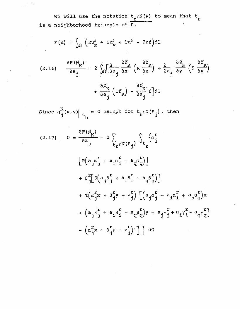
We will use the notation t eN(P) to mean thatr_____is a neighborhood triangle of P.

F(u)

(2.16)

Since g .

(2.17)

= ^ (Ru3 + Su3 + Tu3 - 2 u f W JQ V x y /

s p ( V = 2 r r 3 8_*s 30kn . a 30k0 r a k / k\ a k /jQLda . dx \ dx / + d a . dy \da . ^___ .

3 . 3 3

d0 90 .

3 3

x,y)| t = 0 except for theN(P^), then

dF (0 )

1"r (a .cu + a.af + a ar)l L \ ] ] x i q q / J

+ p T s ( a .pr + a.pr + a pr)lDL \ D : x i q q / J

/ r „r r\ r/ r r+ Tfa.x + p .y + y.) (a.a. + a. a. +\ 3 3 ]/ L\ ] ] i i

/ „r „r\ r r+ ( a . 6 . + a.p. + a p y + a .y . + a . y . + \ 3 3 i i q q/ 3 3 i i

aq

- (a jx + p / + Yj)f] } an

Since R, S, T and f are known, and very often, constantfunctions, we can compute the coefficients of a ., a and

3 qa_ . As was mentioned before, we obtain a system of nequations and n unknowns a_. , one for each interior node j.Note that the form of F(u) shows that if f = 0 on Q, theonly function in M minimizing F(u) is the zero functionKand therefore the solution to the system of equations obtained is unique. One other way to observe the existence and uniqueness of the solution is by theorem 1.3. Since u ., the minimizing element of F(u), is the closest element in in to uq , by theorem 1.3 this element is unique and since that element must satisfy (2.17), then a solution to this system exists. On the other hand the solution to the system (-2.17) minimizes F(u) and therefore is uicand unique.

CHAPTER III UNIFORM CONVERGENCE

Suppose 0 is ah open, simply connected, bounded point set (a region) in the x-y plane. In this section we will study the possibility of the uniform convergence of the finite element approximation to the solution of Poisson's equation, Bu = f (x,y) in Cl and u I = 0, where by dQ we mean the boundary of Q. We start with introducing some necessary definitions, notations and theorems.

Definition 3.1- A function f(x), defined on a bounded closed region of the n-dimensional Euclidean space Rn , is sa-id to be Holder Continuous of exponent g (0 < a < 1) in fi if there is a constant K such that | f (x) - f (y) | <; K | x-y | a for all x and y in fi. The smallest such K is called the Holder Coefficient. A function f(x) is said to be locally Holder Continuous, of exponent a, on an open set Q if, for each closed subset B of Cl there is a constant K(B) such that

| f (x) - f(y) | < K(B) | x-y | a

for every x and y in B. If K(B) is independent of theset B, then f is said to be uniformly Holder Continuousof exponent g .

We denote by cm (Q) the set of all functions whose partial derivatives of all order, up to and including m, are continuous functions in fi. If all of these partial derivatives, and the function itself, are locally

50

Holder Continuous, then we say that the function belongsm+a, * to c (Q).Theorem 3.1 - Let L be any elliptic operator in Q

of the form

,(u) = V a . . (x) -u — + Y b . (x) — - + c (x) u L ii dx. dx. L l dx.n n

d2 u V1 / » duix;ii _. . , i i . . li,1=l J i=l#

where x , i=l,...,n are independent variables. Suppose that f and the coefficients of L, a^ (x) , b^ (x) and c (x) belong to c^,+a(n) (psO), then any solution of Lu = f belongs to c ^ +^ +a(Q) [6 ],

In the special case of the Poisson's equation, the operator B is of the form

(3.1) Bu = - u - u = auxx yyand the variational functional F(u) will have the form

(3.2) F (u) = C (u2 + ua - 2uf)dfi.jn x y

We defined the set M as the set of all polyhedralKfunctions on a triangulation T , vanishing on dT . InK Kfinding the approximate solution u fM by the finiteJc Kelement method, using triangular elements of T , weKminimize the functional (3.2) on M . The minimizingKfunction u^ is obtained by solving the system ofequations dF(0. )/ da. = 0 , where a. is the value ofK 1 1u, at the node P., .i.e., u, (P.) = a.. For each interior k i k i inode A, we obtain one such equation, which we shallcall a nodal equation for the node A.

Let A be an interior node and B^, (r=l,...,n)its neighborhood nodes (Fig. 3.1), and set

a n du. (B ) = a . k r r

Suppose t^ is the triangle made by the sides AB^,B B ,/ B .A and that u, has the form r r+ 1 r+ 1 k

(3’3) \ |tr = (“°a° + “* ar + ar+lar+l)x

+ (p ? « o + + e r +1a^+ 1 ) y

r r r+ ao Yo + a Y + a iY n r 1r r+l'r+l

on triangle t (see equation 2 .1 2 ), where r+ 1 = 1 when r=n Then the nodal equation for the node A as obtained from equation (’2.17) is of the form

n

(3'4) I Ar [ + arar + V l V l Kr=l

/ ^r r r \0ri+ (aoPo + V r + ar+1 er+1)PoJ

nv p / r r r\

= £ ct0 x + p0 y + Y o j f d n

r=l rn

“ I St gAfdCi1 r r=l

where A^ denotes the area of t^. Using the geometry of the triangles and assuming 0^ is the counter clock­wise angle made by the x-axis and AB , B and Br r,r r+l,rare the angles AB B and AB B respectively,r r+l r+ 1 r(Pig. 3.2), we obtain

B B . sin (0 - B )r _ r r+ 1____ __r____ r , raA “ 2(Area t )

B B . cos(0 - B ) r _ r r+ 1 _ r ____ r , rA ~~ 2(Area of t )

t rSubstituting these and similar expressions for (3 , a ,IT 3TP and a into equation (3.4) we obtain r+ 1 r+ 1

n B B cot B , + cot B . _V r r+ 1 _ r+l,r * r-l,r-l _ pI “Sir- a° - - - - - - - - S- - - - - - - - r “

r=1 r

where h is the altitude of triangle t from the node A r rto the side B B Since g„(x,y) £ 0 then we canr r+1 Awrite n

JjgA fdfi = f(x0 ,y0 ) = f(x0 ,y0 ) j £ Area of t^ ,r=l

where (x0 ,y0 ) is a point in one of the neighborhood triangles of A. Letting F(A) = f(Xo,y0 ) we have

In B B n cot B .. + cot B . ,r r+ 1 r+l,r r-l,r-l

2h a° 2 arr=l r

= ^ - F ( A ) .

where S(A) is the total area of the neighborhood triangles of A.

Note that

B B . cot B + cot B . r r+1 r, r r+1 , r2hr 2

a n d t h e r e f o r e

cot Br+1 , r + cot B2

r-1 ,r- 1

A Special Triangulation

We will prove the uniform convergence of the approximation u to the solution of Bu = f for a specialK V

type of triangulation. In this type of triangulation we will assume that all angles equal to 60°. One simple and practical way to obtain this kind of triangulation is to have 3 classes of parallel lines , the lines of each class intersecting the lines of the two others at 60° angles Fig. (3.3). The lines of each class are separated by a predecided length h. Now if a line of the third class passes through the intersection of every two lines of the first two classes, then we obtain a grid desirable for the triangulation needed. The grid obtained consists of equilateral triangles and therefore for every vertex A of a triangle of the grid, there are exactly 6 neighborhood triangles of A. The triangular cover of the region Q, as defined in Chapter 2, is obtained from the triangles of this grid. Note that here again we do not require the convexity of the region and therefore the region obtained by the triangles of the triangulation is not necessarily a connected set. Also note that the boundary nodes are not necessarily on the boundary of Q.

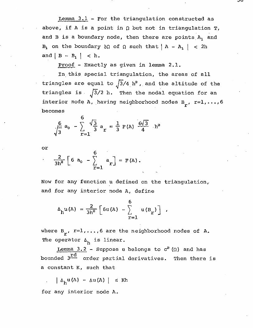
Lemma 3.1 - For the triangulation constructed as above, if A is a point in fi but not in triangulation T, and B is a boundary node, then there are points Ax and Bi on the boundary BQ of Q such that | A - Ax | < 2hand | B - Bx | < h.

Proof - Exactly as given in lemma 2.1.In this special triangulation, the areas of all

triangles are equal to ^3/4 ha , and the altitude of the triangles is h. Then the nodal equation for aninterior node A, having neighborhood nodes B^, r=l, . . . , 6 becomes

6

r=l

or 62[6 a ° - I ar] = p (a >-3h r=l

Now for any function u defined on the triangulation, and for any interior node A, define

6V ' fl)=3 M 6u(A)- I u(Br>] '

r=l

where B^, r=l, . . . , 6 are the neighborhood nodes of A.The operator is linear.

Lemma 3.2 - Suppose u belongs to c3 (Q) and has rdbounded 3— order partial derivatives. Then there is

a constant K, such that

| Ahu(A) - Au(A) | <; Kh

for any interior node A.

Proof - Let A be any interior node with (r=l,6 ) denoting its neighborhood nodes. Suppose 0^ is the counterclockwise angle between the x-axis and AB^ (Fig. 3.4). Note that

er = e, + (r-i) 3. .Suppose the coordinates of A are x , y , then for pointa aE (x ,y ) r r Jr

x = x + h cos 0r a r 'y = y + h sin 0r a r

Expanding the function u by Taylor's formula about thepoint A (x ,y ) we obtain a a

u(B ) = u(A) + h cos 0 u (A) + h sin 0 u (A) r r x r yu (A) h2 sin2 0 h2sin 0 cos 0

+ hscos2 er -§^ + --- ---------------T ” uxy ’

+ Rg .

rdSince the 3— order partial derivatives of u are bounded, say by Kj , then

Rs I ^ Ki/ .h3 = Ki/ h33 1 / 3 ' Ve

Expanding u(B ) , for every r, about point A and taking r 6

the summation ^ u(B^), we obtainr=l

Figure 3.4

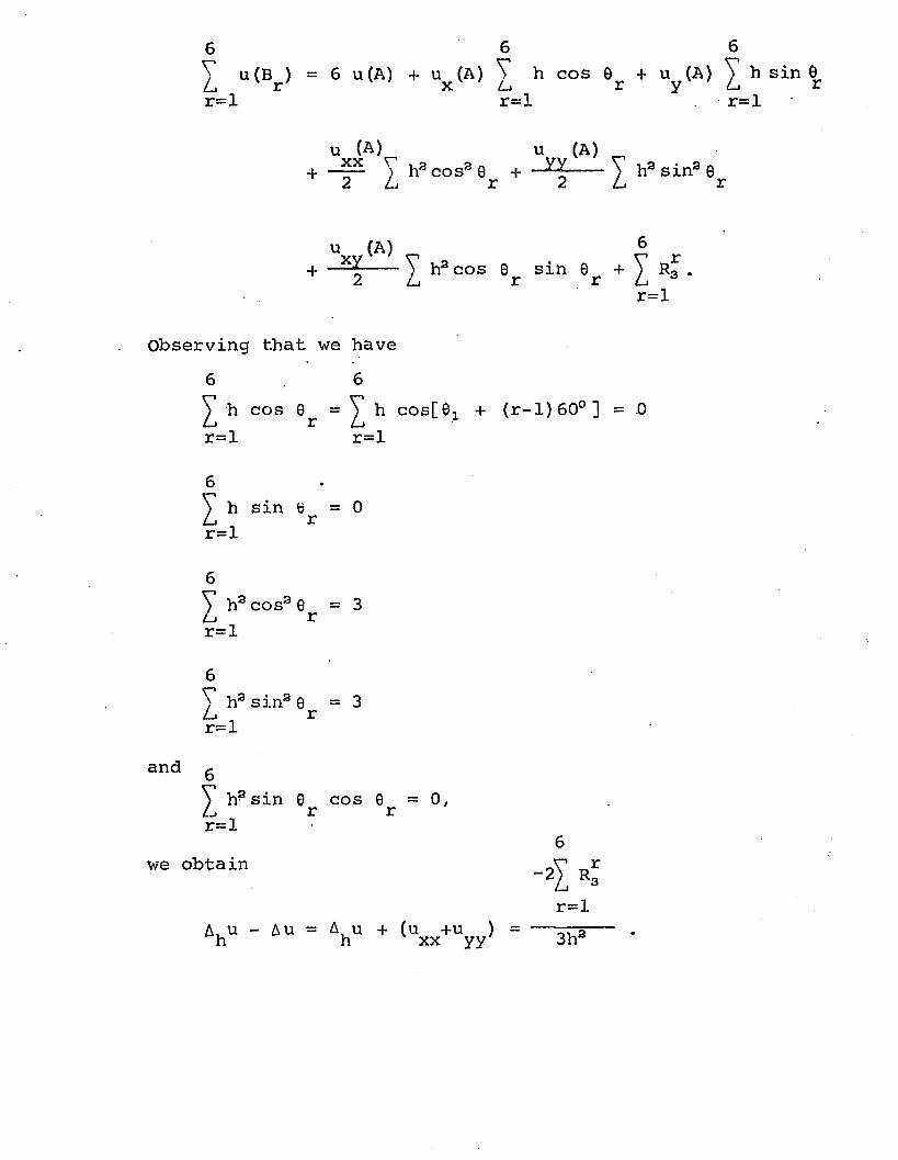
^ u (Br) = 6 u(A) + Ux (A) I h cos 0^ + u^(A) ^ h sin 6, r=l r=l r=l

u (A) u (A)+ "~V* Y cosa 9 + ’~ ^ r — y sin3 ®2 Li r 2 Lj r

u (A) B+ £ ha cos 0r sin ®r + ^ R 3

r=l

Observing that we have 6 6^ h cos 0r = ^ h cosC©! + (r-l)60°] = .0 r=l r=l

Ih sin B = 0 r r=l

^ ha cosa 0^ = 3r=l

6V h3 sin3 0 = 3L rr=l

and 6

Y h3sin 0 cos 0 = 0 ,L r rr=l 6

we obtain nr3- 2l

r=lA, u - Au = A u + (u +u ) = — . h h xx yy 3ha

Since6 6

l£ r3 i * £l 41 * Kxh3 ,r=l r=l

we finally have the stated result,

2| A^u - Au | £ — Kx h .

Lemma 3.3 - (Maximum Principle) Suppose v is apolyhedral function, i.e., v is linear on each triangleof the triangulation. Also suppose that for eachinterior node A, A, v(A) 0. Then v takes on itshmaximum on a boundary node.

Proof - Since v is linear on each triangle, it attains its maximum on that triangle at a vertex of the triangle, i.e., a node. Now suppose contrary to the lemma, there is an interior node A having boundary nodes B^, (r=l,...,6 ) such that v(A) > v(B^) for some1 s j <s 6 and v(A) £ v (Br) (r=l,...,6 ). Then

6v (A) = 3^ [ 6v(a) - I v(v ]r=l

> 3 ^ [ Z v(v - I v(V j = or-l r=l

This is contrary to the assumption A^v(A) <: 0.The finite element approximation is obtained by

solving the nodal equations which are themselves theresult of minimizing the functional

, . C(ua + u2 - 2uf)dfi F(u) = ^ x y

in the space M of all polyhedral functions defined on . Kthe given triangulation. If f is the zero function,then the only function minimizing this functional is thezero function, which states that the only solution tothe system of homogeneous nodal equations is the zerofunction. By a well-known theorem in linear algebra,this implies that the solution to the system of nodalequations and equations expressing'the boundary valuesis unique, i.e., the system A^u(A) = F(A) for an interiornode A and u(B) = a_ for a boundary node B, has aBunique solution.

At this stage' we introduce the finite element analogue of the Green's function. Define

6 <P 'Q> “ { I if P Q

for any two points P and Q of the triangulation. For a given point P, suppose G^(P,Q) is the unique solution to the system of equations

A^G^P/Q) = if Q is an interior node

G^(P,Q) = 6 (P,Q) if Q is a boundary node.

Suppose also that G^ is linear on each triangle and therefore is a polyhedral function.

Denote the set of all interior nodes of a triangulation T, by I(T).

Lemma 3.4 - Let v be a polyhedral function defined on the triangulation under study, then for any interior

node A,

v (A) = h2 £ Gh (A,c) [Ahv(c)] . c d (T)

Proof - Define a polyhedral function w(A) in the following way: for a boundary node B, let w(B) = v(fi)and for an interior node P, let

w(P) = h2 £ Gh (P,Q) [Ahv(Q)J .Qel(T)

Then since A^ is a linear operator

V (P) = Aj, [h« I Gh (P,Q) *hv(Q)]QeKT)

= h3 I Ahv (Q) AhGh (P,Q) •QeKT)

Since6 (P/Q)

then

AhGh (P,Q) =

Ahw.(P) = Ahv(P) .

Therefore w and v both are the solution of the system of nodal equations A^u(A) = = A^v(A) for the interiornode A and u(B) = v(B) on the boundary nodes B. Since the solution to this system is unique, we have w(P) = v(P) for all points P. For interior nodes A,

v(A) = w(A) = h3 £ Gh (A,C) [Ahv(c)]ccX(T)

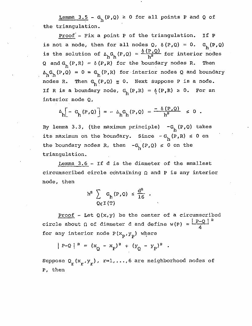
Lemma 3.5 - G^(P,Q) £: 0 for all points P and Q ofthe triangulation.

Proof'- Fix a point P of the triangulation. If Pis not a node, then for all nodes Q, 6 (P,Q) = 0. G, (P,Q)is the solution of A, G. (P,Q) = — — ~ for interior nodesh h h*3Q andGh (PjR) = 6 (P,R) for the boundary nodes R. ThenA,G, (P.Q) = 0 = G. (P,R) for interior nodes Q and boundary h h hnodes R. Then G^(P,Q) = 0. Next suppose P is a node.If R is a boundary node, G^(P,R) = 6 (P,R) ^ 0. For an interior node Q,

V P>Q)] ■ - AhGh(p'Q) = ~ h ^ 4 0 •By lemma 3.3, (the maximum principle) -G^(P,Q) takesits maximum on the boundary. Since -G^(P,R) ^ 0 onthe boundary nodes R, then -G^(P,Q) s 0 on thetriangulation.

Lemma 3 .6 - If d is the diameter of the smallest circumscribed circle containing Q and P is any interior node, then

h 3 1 < y p'Q) s f ? •QeKT)

Proof - Let Q(x,y) be the center of a circumscribedI p_Q I acircle about 0 of diameter d and define w(p) = '— -— 1fr

for any interior node P(xp/yp) where

| P-Q |a = <xQ - xp )2 + (yQ - yp)a .

Suppose Q (x ,y ), r=l, . . . , 6 are neighborhood nodes of P , then

V (P) “ 3 ^ [ 6W(I,) ~1 WiQi)]i=l

66h*= [ 6 | P-Q | a - £| Qr-Q | ■»]

r=lSince

x = x + h cos 0 r p ]

. y = y + h sin 0 r p r

where 0^ is the counterclockwise angle made by the x-axis and the line PQr' then we have

I I V Q | 2 (xr " V + <yr-yQ>r=l r=l

= I (XP_XQ+ h COS 9r)2 + (yP~yQ + hr=l

- 6 [ < V * Q > ‘ + ‘V V * ]6 6

+ 2h(xp“xQ)^cos 0r+ 2h(yp-yQ )^sin 0 r=l r=l

= 6 I P-Q I 3 + 6ha .

Therefore

>hw(P) = ^ r [ - 6h»] - - i

sin 0 )a r

+ 6ha

for all interior nodes p.

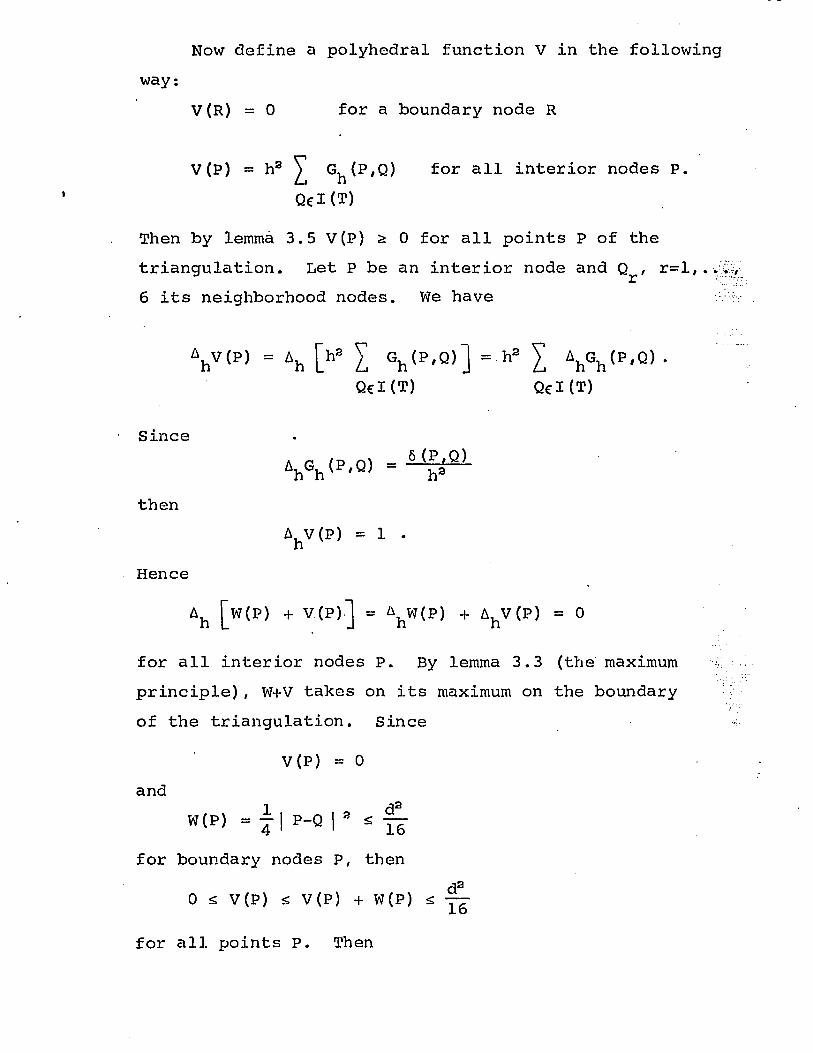
Now define a polyhedral function V in the followingway:

V (R) = 0 for a boundary node R

V (P) = h3 ^ G^(P/Q) for all interior nodes P.QeKT)

Then by lemma 3.5 V(P) ^ 0 for all points P of the triangulation. Let P be an interior node and Q , r=l, . . 6 its neighborhood nodes. We have

V (p) ■ ah [h21 Gh (p-Q)] -■h31 AhGh (p'Q)-QeKT) Qel(T)

Since

then

Hence

AhGh (P,Q)

AhV(P) = 1 .

Ah [w(P) + V(P)~| = Ahw(P) + AhV(P) = 0

for all interior nodes P. By lemma 3.3 (the maximum principle), W+V takes on its maximum on the boundary of the triangulation. Since

V(P) = 0and

W(P) = i I P-Q I 3 s f i

for boundary nodes P, thenj2

0 :£ V(P) <; V(P) + W(P) £ —lbfor all points P. Then

h3 £ Gh (P,Q) = V(P) £ —

QcI(T)

for any interior node P.Theorem 3.2 - Let f be a continuous function having

bounded first order partial derivatives on fi. Suppose u0 is the exact solution of the Poisson's equation

d3 u d2 u x- Au = i ^ + a p - =-f (x 'y) on a

andu = 0 on dfi

and u is the approximate solution obtained by the finiteelement method using a triangulation all of whose trianglesare equilateral. Then if u0 belongs to ca (Q) and has

rdbounded 3— order partial derivatives, there1 is a constant c0 , such that

| u0 (x,y) - uR (x,y) | < c0h

for all points (x,y) in the region fi.Proof - By lemma 3.2 | A, u0 (A) - Au0 (A) | < h

2for an interior node A , where K, = — K 1, K 1 being the rdbound for 3— order partial derivatives. Note that since

rdQ is a bounded region and the 3— order partialnd stderivatives of u0 are bounded, then the 2— and 1—

orders which are continuous will also be bounded. Lets t%K2 be the bound for the 1— order partial derivatives,

thenr 'Yl * , dun ,U0 (*1 , yx ) - u0 (x0 , y0 ) = ^ dx + dy .(xo • y0 )

Therefore if | (x^yj) - (Xp/y0 ) | £ h, we have

| (X£ , yt) - u0 (Xq ,y0) | < K3h .

For the triangulation under study, by lemma 3.1, to any boundary node A there is a point P on dn such that | A-P | < h and therefore , since u^(A)=Uo (P)=0, we obtain

(3.1) | ur (A) - u0 (A) | = | u0 (A) | •= | u0 (A) - u0 (P) | < K2h .

\Also if P is a point in a triangle and A a vertexof the same triangle, then| u0 (P) - u0 (A) | < K2 h .

Now let v represent a polyhedral function definedon the triangulation by v(A) = u (A) - u0 (A) for anyKnode A. By lemma 3.4

(3.2) v(A) = h2 £ Gh (A,o) [Ahv(c)]ce I(T)f

for all interior nodes A. Also

AhuK (A ) = F(A) = f(x0 ,y0 )

= f(A) - [f (A) - f (x0 ,y0)]

= &u0 (A) - (A) - ffXo.yj]

where, as seen before, (x0 ,y0 ) is some point in one of the neighborhood triangles of A and therefore

s t|C^o»Yo) - ^ | < h. Supposing the bound of the 1—derivatives of f is K3 , we have

| f (A) - f (Xq ,y0 ) | < K 3h .

We also find that(3.3) Ahv(A) = AhUK (A) - A ^ (A) = Au0 (A) - (A)

- (A) - f (Xq ,y0 ) Jand therefore ::

| Ahv(A) | ^ | Au0 (A) - Ahu0 (A) | + | f(A) - f (x0 ,y0 )

< (Kx + K 3 ) h .

Thus, for an interior node A

| v(A) | = | ha £ Gh (A,c) A^vCc)ccI(T)

< (Kx + K3 ) h | h8 ^ Gh (A,c)

By lemma 3 .6

I hS Z Gh (A'C) | 3J •c€I(T)

Thusda(3.4) | v (A) | s (Kx + Ka) h 16

r ds ^for an interior node A. If K4 = max | (Kx + K3 Jyg-# Kajthen equations (3.1) and (3.4) imply that for any nodeA, we have

| v(A) | ur (A) - u0 (A) | < K4h .

Now suppose D is a point of Q and D is not a node. IfD is not a point of the triangulation, then by lemma 3.1 there is a point P on the boundary of fi such that | D-P | < 2h and therefore

uk (D) - u0 (D) | =| u0 (D) | : =-|; ub (35) - u0 (P) | <; 2K3h.

If D is a point of the triangulation, but not a node,then D belongs to some triangle t . Since u is linearr Kon t , it attains its maximum and its minimum on the rvertices of t . Let A and B be two vertices of t such r rthat u (B) £ u (D) u (A). Then since ;;K K K i

| uk (b) “ u0 (B) | < K4h

and| Uq (B) - u0 (D) | < Kah

we obtain

uk (b).- U0 (D) = [uk (B) - u0 (B)] + [u0 (B) - u0 (D)J

> - K4h - Kah > - 2K4 h.

Also we find thatUK (A) - u0 (D) = [uk (a ) “ u0 (A)J + [u0 (A) - u0 (D)]

i 1< K4 h + K3h <; 2k4 h .

Therefore

- 2K4h < uk (B) - u0 (D) < uk (D) - u0 (D)

< uk (a) " u° ^ < 2K4h*

Thus| UK (°) - uo (D) | < 2K4 h.

f ■ da iIF c0 = max |2(K^ + K3) — , 2Kaj, then for any point Pon Q we have .-%v • ;

This theorem proves, not only the uniform convergence of the approximate solution to the exact solution but, gives a bound for the error in terms of the length of the sides of the triangles of the triangulation.

REFERENCES

1 .

2.

3.

4.

5.

6 .

7.

8.

9.

10.

Akhiezer, N. I. and Glazman, I. M. Theory of Linear Operators in Hilbert Space Volume I_. Frederick Ungar Publishing Co., New York, 1961.

Bramble, J. H. and Hubbard, B. E. On the Formulation of Finite Difference Analogues of the Dirichlet Problem for Poisson's Equation. Numerische Mathematik, 4B and 4 Heft> December 1962, 313-327.

Courant, R. and Hilbert D. Methods of Mathematical Physics Vol. II. Intersciences Publishers,New York, N. Y., 1962.

Crandall, S. H. Engineering Analysis. McGraw- Hill Book Co., New York, 1956.

Flippa, c. A. and Clough, R. W. The Finite Element Method in Solid Mechanics. Proceeding of the Symposium on Numerical Solutions of Field Problems in Continuum Mechanics, April 5-6, 1968.

Friedman, A. Partial Differential Equations of Parabolic Type. Prentice Hall, Inc. 1964.

Key, S. W. A Convergence Investigation of theDirect Stiffness Method, A Ph.D. Dissertation, University of Washington, 1966.

Mikhlin, S. G. The Problem of The Minimum of a Quadratic Functional. Holden-Day, Inc.San Francisco, Calif., 1965.

Mikhlin, S. G. Variational Methods in Mathematical Physics. Macmillan Co., New York, N. Y., 1964.

Oden, J. T. A General Theory of Finite Elements, I-Topological Considerations. International Journal of Numerical Methods in Engineering,Volume 1, 205-221, (1969).

71

11. Synge, J. L. The Hypercircle in Mathematical Physics.Cambridge University Press, Cambridge, 1957.'

12. Zienkiewicz, O. C. and Cheung, Y. K. The FiniteElement Method in Structural and Continuum Mechanics. McGraw-Hill Publishing Company Limited. New York, N. Y. 1967.

VITA

Nasrollah Tabandeh was born in Bidokht, Iran in 1934. He was graduated with a mathematics major from Fiouzat High School, Mashhad, Iran in 1952. Afterward he attended the University of Tehran and graduated with a "Mechanical Engineer" degree in 1956. He entered Louisiana State University in 1959 and received his Master of Science degree in Mechanical Engineering in 1961. In 1965,.he reentered Louisiana State University and received his Master of Science: degree in Mathematics in 1968. At the present time,".he is^aK candidate of the degree of Doctor of Philosophy in the'Deparf^t of Engineering Science of Louisiana State University'.

EXAMINATION AND THESIS REPORT

Candidate: Nasrollah Tabandeh

Major Field: Engineering Science

Title of Thesis: Convergence of the Finite Element Method

Approved:

ajor Professor and Chairman

Dean of the Graduate School

EXAMINING COMMITTEE:

W t \

Jl

Date of Examination:

May 29, 1970