Convergence in (Social) Influence Networks

Silvio Frischknecht, Barbara Keller, and Roger Wattenhofer

Computer Engineering and Networks Laboratory (TIK), ETH Zurich, Switzerlandfsilvio,barkelle,wattenhofer@tik.ee.ethz.ch

Abstract. We study the convergence of influence networks, where each nodechanges its state according to the majority of its neighbors. Our main result is anew Ω(n2/ log2 n) bound on the convergence time in the synchronous model,solving the classic “Democrats and Republicans” problem. Furthermore, we givea bound of Θ(n2) for the sequential model in which the sequence of steps isgiven by an adversary and a bound ofΘ(n) for the sequential model in which thesequence of steps is given by a benevolent process.

1 Introduction

What do social networks, belief propagation, spring embedders, cellular automata, dis-tributed message passing algorithms, traffic networks, the brain, biological cell systems,or ant colonies have in common? They are all examples of “networks”, where the enti-ties of the network are continuously influenced by the states of their respective neigh-bors. All of these examples of influence networks (INs) are known to be difficult toanalyze. Some of the applications mentioned are notorious to have long-standing openproblems regarding convergence.

In this paper we deal with a generic version of such networks: The network is givenby an arbitrary graph G = (V,E), and all nodes of the graph switch simultaneously tothe state of the majority of their respective neighbors. We are interested in the stabilityof such INs with a binary state. Specifically, we would like to determine whether anIN converges to a stable situation or not. We are interested in how to specify sucha stable setting, and in the amount of time needed to reach such a stable situation. Westudy several models how the nodes take turns, synchronous, asynchronous, adversarial,benevolent.

Our main result is for synchronous INs: Each node is assigned an initial state from theset R,B, and in every round, all nodes switch their state to the state of the major-ity of their neighbors simultaneously. This specific problem is commonly referred toas “Democrats and Republicans”, see e.g. Peter Winkler’s CACM column [Win08]. Itis well known that this problem stabilizes in a peculiar way, namely that each nodeeventually is in the same state every second round [GO80]. This result can be shownby using a potential bound argument, i.e., until stabilization, in each round at least onemore edge becomes “more stable”. This directly gives a O(n2) upper bound for theconvergence time. On the other hand, using a slightly adapted linked list topology, onecan see that convergence takes at least Ω(n) rounds. But what is the correct bound for

this classic problem? Most people that worked on this problem seem to believe that thelinear lower bound should be tight, at least asymptotically. Surprisingly, in the courseof our research, we discovered that this is not true. In this paper we show that the upperbound is in fact tight up to a polylogarithmic factor. Our new lower bound is based ona novel graph family, which has interesting properties by itself. We hope that our newgraph family might be instrumental to research concerning other types of INs, and mayprove useful in obtaining a deeper understanding of some of the applications mentionedabove.

We complement our main result with a series of smaller results. In particular, we lookat asynchronous networks where nodes update their states sequentially. We show thatin such a sequential setting, convergence may take Θ(n2) time if given an adversarialsequence of steps, and Θ(n) if given a benevolent sequence of steps.

2 Related Work

Influence networks have become a central field of study in many sciences. In biology,to give three examples from different areas, [RT98] study networks in the context ofbrain science, [AAB+11] study cellular systems and their relation to distributed al-gorithms, and [AG92] study networks in the context of ant colonies. In optimizationtheory, believe propagation [Pea82, BTZ+09] has become a popular tool to analyzelarge systems, such as Bayesian networks and Markov random fields. Nodes are con-tinuously being influenced by their neighbors; repeated simulation (hopefully) quicklyconverges to the correct solution. Belief propagation is commonly used in artificialintelligence and information theory and has demonstrated empirical success in numer-ous applications such as coding theory. A prominent example in this context are thealgorithms that classify the importance of web pages [BP98, Kle99]. In physics andmechanical engineering, force-based mechanical systems have been studied. A typicalmodel is a graph with springs between pairs of nodes. The entire graph is then simu-lated, as if it was a physical system, i.e. forces are applied to the nodes, pulling themcloser together or pushing them further apart. This process is repeated iteratively untilthe system (hopefully) comes to a stable equilibrium, [KK89, Koh89, FER91, KW01].Influence networks are also used in traffic simulation, where nodes (cars) change theirposition and speed according to their neighboring nodes [NS92]. Traffic networks of-ten use cellular automata as a basic model. A cellular automaton [Neu66, Wol02] is adiscrete model studied in many fields, such as computability, complexity, mathematics,physics, and theoretical biology. It consists of a regular grid of cells, each in one of afinite number of states, for instance 0 and 1. Each cell changes its state according to thestates of its neighbors. In the popular game of life [Gar70], cells can be either dead oralive, and change their states according to the number of alive neighbors.

Our synchronous model is related to cellular automata, on a general graph; however,nodes change their opinion according to the majority of their neighbors. As majorityfunctions play a central role in neural networks and biological applications this modelwas already studied during the 1980s. Goles and Olivos [GO80] have shown that asynchronous binary influence network with a generalized threshold function always

leads to a fixed point or to a cycle of length 2. This means that after a certain amount ofsynchronous rounds, each participant has either a fixed opinion or changes its mind inevery round. Poljak and Sura [PS83] extended this result to a finite number of opinions.In [GT83], Goles and Tchuente show that an iterative behavior of threshold functionsalways leads to a fixed point. Sauerwald and Sudholt [SS10] study the evolution of cutsin the binary influence network model. In particular, they investigate how cuts evolveif unsatisfied nodes flip sides probabilistically. To some degree, one may argue that welook at the deterministic case of that problem instead.

In sociology, understanding social influence (e.g. conformity, socialization, peer pres-sure, obedience, leadership, persuasion, sales, and marketing) has always been a cor-nerstone of research, e.g. [Kel58]. More recently, with the proliferation of online socialnetworks such as Facebook, the area has become en vogue, e.g. [MMG+07, AG10].Leskovec et al. [LHK10] for instance verify the balance theory of Heider [Hei46] re-garding conformity of opinions; they study how positive (and negative) influence linksaffect the structure of the network. Closest to our paper is the research dealing withinfluence, for instance in the form of sales and marketing. For example, [LSK06] in-vestigate a large person-to-person recommendation network, consisting of four millionpeople who made sixteen million recommendations on half a million products, andthen analyze cascades in this data set. Cascades can also be studied in a purely theoret-ical model, based on random graphs with a simple threshold model which is close toour majority function [Wat02]. Rumor spreading has also been studied algorithmically,using the random phone call model, [KSSV00, SS11, DFF11]. Using real data fromvarious sources, [ALP12] show that networks generally have a core of influential (elite)users. In contrast to our model, nodes cannot change their state back and forth, onceinfected, a node will stay infected. Plenty of work was done focusing on the predictionof influential nodes. One wants to find subset of influential nodes for viral marketing,e.g. [KKT05, CYZ10]. In contrast, [KOW08] studies the case of competitors, which iscloser to our model since nodes can have different opinions. However, also in [KOW08]nodes only change their opinion once. However, in all these social networks the under-lying graph is fixed and the dynamics of the stabilization process takes place on thechanging states of the nodes only. An interesting variant changes the state of the edgesinstead. A good example for this is matching. A matching is (hopefully) convergingto a stable state, based on the preferences of the nodes, e.g. [GS62, KPS10, FKPS10].Hoefer takes these edge dynamics one step further, as not only the state of the edgechanges, but the edge itself [Hoe11].

3 Model Definition

An influence network (IN) is modeled as a graph G = (V,E, o0). The set of nodesV is connected by an arbitrary set of edges E. Each node has an initial opinion (orstate) o0(v) ∈ R(ed), B(lue). A node only changes its opinion if a majority of itsneighbors has a different opinion. One may consider several options to breaking ties,e.g., using the node’s current opinion as a tie-breaker, or weighing the opinions of indi-vidual neighbors differently. As it turns out, for many natural tie-breakers, graphs can

be reduced to equivalent graphs in which no tie breaker is needed. For instance, usinga node’s own opinion as a tie-breaker is equivalent to cloning the whole graph, andconnecting each node with its clone and the neighbors of its clone.

In this paper we study both synchronous and asynchronous INs. The state of a syn-chronous IN evolves over a series of rounds. In each round every node changes its stateto the state of the majority of its neighbors simultaneously. The opinion of a node v inround t is denoted as ot(v).

As will be explained in Section 5, the only interesting asynchronous model is the se-quential model. In this model, we call the change of opinion of one node a step. Theopinion of node v after t steps is defined as ot(v). In general, more than one node maybe ready to take a step. Depending on whether we want convergence to be fast or slow,we may choose different nodes to take the next step. If we aim for fast convergence, wecall this the benevolent sequential model. Slow conversion on the other hand we call theadversarial sequential model.

We say that an IN stabilizes if it reaches a state where no node will ever change itsopinion again, or if each node changes its opinion in a cyclic pattern with periodicity q.In other words, a state can be stable even though some nodes still change their opinion.

Definition 1. An IN G = (V,E, o0) is stable at time t with periodicity q, if for allvertices v ∈ V : ot+q(v) = ot(v). A fixed state of an IN G is a stable state withperiodicity 1. The convergence time c of an IN G is the smallest t for which G is stable.

Note that since INs are deterministic an IN which has reached a stable state will staystable.

In this paper we investigate the stability, the convergence time c and the periodicity qof INs in the described models. Clearly, the convergence process depends not only onthe graph structure, but also on the initial opinions of the nodes. We investigated graphsand initial opinions that maximize convergence time. In the benevolent sequential inparticular, we investigate graphs and sets of initial opinions leading to the worst possibleconvergence time, given the respectively best sequence of steps.

4 Synchronous IN

A synchronous IN may stabilize in a state where some nodes change their opinion inevery round. For example, consider the graph K2 (two nodes, connected by an edge)where the first node has opinionB and the second node has opinionR. After one round,both vertices have changed their state, which leads to a symmetric situation. This INremains in this stable state forever with a period of length 2. As has already been shownin [GO80, Win08], a synchronous IN always reaches a stable state with a periodicity ofat most 2 after O(n2) rounds.

Theorem 1 ([Win08]). A synchronous IN reaches a stable state after at most O(n2)rounds.

Theorem 2 ([GO80]). The periodicity of the stable state in a synchronous IN is at most2.

In this paper, we prove this bound to be almost tight.

Theorem 3. There is a family of synchronous INs with convergence timeΩ(

n2

(log logn)2

).

Unfortunately, the technical proof of Theorem 3 does not fit into this paper. You canfind the full proof in Appendix A. In this section, we instead present a simpler IN withconvergence time Ω

(n3/2

).

The basic idea is to construct a mechanism which forces vertices on a simple path graphto change their opinion one after the other. Every time the complete path has changed,the mechanism should force the vertices of the path to change their opinions back againin the same order. To create this mechanism, we introduce an auxiliary structure calledtransistor, which is depicted in Figure 1.

B2

B3

E3B1 E1

C1 C3

E0 E2

C2C0

Fig. 1: A transistor T (4). The dotted lines indicate how the transistor will be connected.

Definition 2. A transistor of size k, denoted as T (k), is an undirected graph consistingof k collector vertices C = Ci | 0 ≤ i ≤ k−1, k emitter vertices E = E i | 0 ≤ i ≤ k−1and three base vertices B = B1,B2,B3. All edges between collector and emitter ver-tices, all edges between any two base vertices, and all edges between collector verticesand the third base vertex exist. Formally:

T (s) =(V,E)

V =C ∪ E ∪ BE =u, v | u ∈ C, v ∈ E ∪ u,B3 | u ∈ C∪u, v | u, v ∈ B, u 6= v

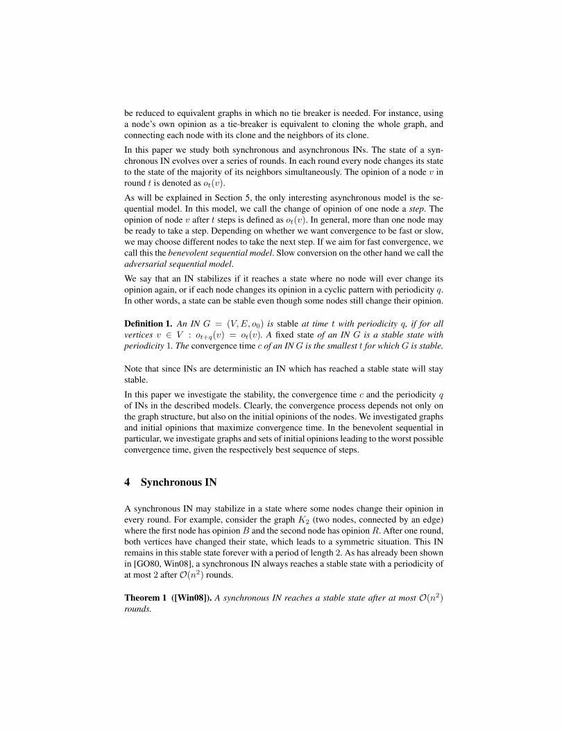
All nodes in a transistor are initialized with the same opinion X ∈ R = 1, B = −1.The 3 + k + k2 collector edges (dotted edges pointing to the top of Figure 1, includingthose originating from B1,B2 and B3) are connected to vertices with the constant opin-ion −X , while up to k2 − k emitter edges (dotted edges pointing to the bottom) andthe 2 base edges (dotted edges pointing to the left) may be connected to any vertex. Assoon as both base edges advertise opinion−X , the transistor will flip to opinion−X in4 rounds regardless of what is advertised over the emitter edges, i.e., the following setsof vertices will all change their opinion to −X in the given order: B1, B2,B3, C,E .

TR1

Fig. 2: Path with 4 vertices connectedto one transistor T (3).

TR1

T0B T

2B

Fig. 3: Path with 4 vertices connectedto 3 transistors T (3). Note that transis-tors at bottom of figures are always up-side down.

TR1

T1B

TR2

T0R

T0B T

2B

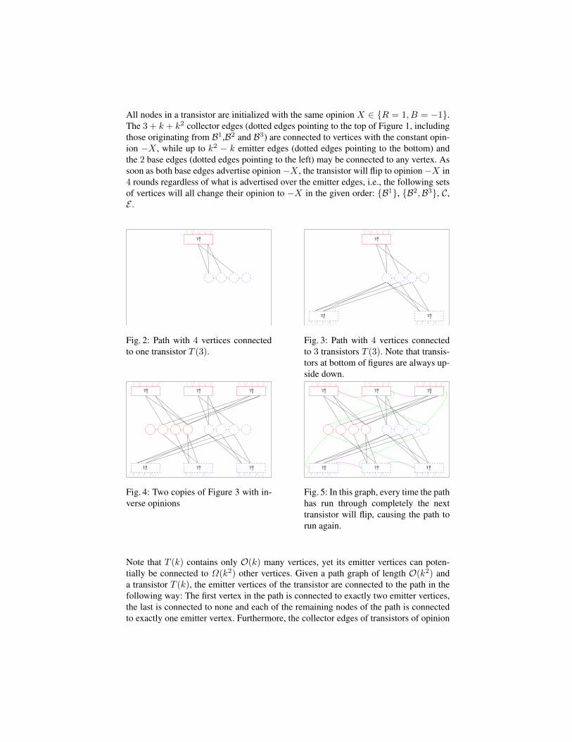
Fig. 4: Two copies of Figure 3 with in-verse opinions

TR1

T1B

TR2

T0R

T0B T

2B

Fig. 5: In this graph, every time the pathhas run through completely the nexttransistor will flip, causing the path torun again.

Note that T (k) contains only O(k) many vertices, yet its emitter vertices can poten-tially be connected to Ω(k2) other vertices. Given a path graph of length O(k2) anda transistor T (k), the emitter vertices of the transistor are connected to the path in thefollowing way: The first vertex in the path is connected to exactly two emitter vertices,the last is connected to none and each of the remaining nodes of the path is connectedto exactly one emitter vertex. Furthermore, the collector edges of transistors of opinion

TR1

T1B

TR2

T0R

T0B T

2B

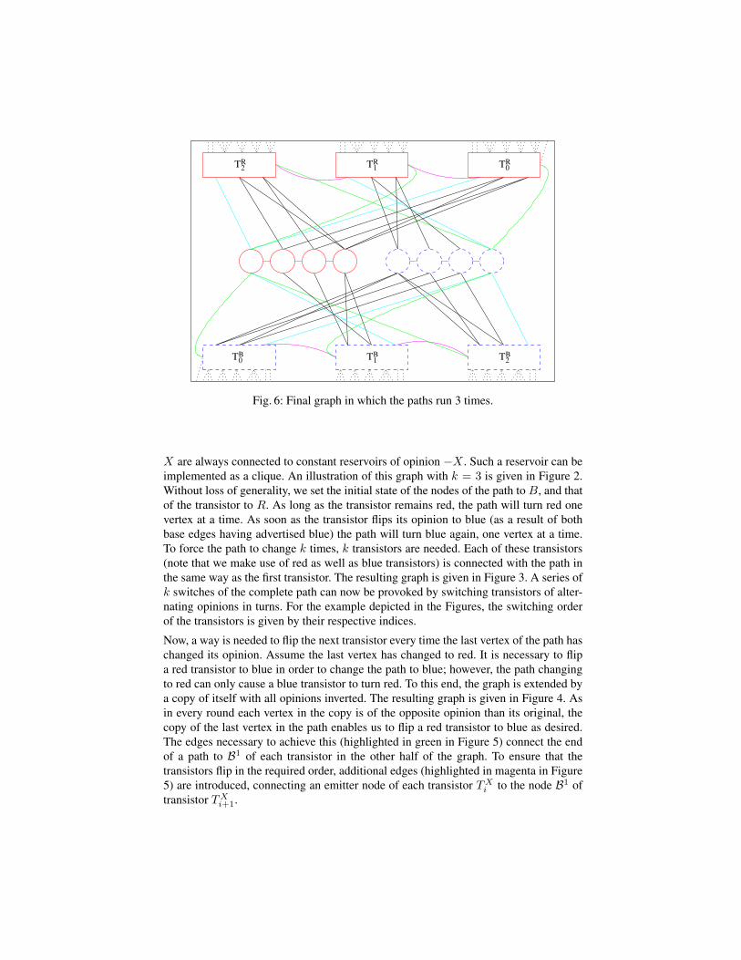
Fig. 6: Final graph in which the paths run 3 times.

X are always connected to constant reservoirs of opinion −X . Such a reservoir can beimplemented as a clique. An illustration of this graph with k = 3 is given in Figure 2.Without loss of generality, we set the initial state of the nodes of the path to B, and thatof the transistor to R. As long as the transistor remains red, the path will turn red onevertex at a time. As soon as the transistor flips its opinion to blue (as a result of bothbase edges having advertised blue) the path will turn blue again, one vertex at a time.To force the path to change k times, k transistors are needed. Each of these transistors(note that we make use of red as well as blue transistors) is connected with the path inthe same way as the first transistor. The resulting graph is given in Figure 3. A series ofk switches of the complete path can now be provoked by switching transistors of alter-nating opinions in turns. For the example depicted in the Figures, the switching orderof the transistors is given by their respective indices.

Now, a way is needed to flip the next transistor every time the last vertex of the path haschanged its opinion. Assume the last vertex has changed to red. It is necessary to flipa red transistor to blue in order to change the path to blue; however, the path changingto red can only cause a blue transistor to turn red. To this end, the graph is extended bya copy of itself with all opinions inverted. The resulting graph is given in Figure 4. Asin every round each vertex in the copy is of the opposite opinion than its original, thecopy of the last vertex in the path enables us to flip a red transistor to blue as desired.The edges necessary to achieve this (highlighted in green in Figure 5) connect the endof a path to B1 of each transistor in the other half of the graph. To ensure that thetransistors flip in the required order, additional edges (highlighted in magenta in Figure5) are introduced, connecting an emitter node of each transistor TX

i to the node B1 oftransistor TX

i+1.

The green edges cause an unwanted influence on the last vertex of the paths. This influ-ence can be negated by introducing additional edges (highlighted in cyan in Figure 6).These edges connect the last vertex of each path with an emitter vertex of each transistornot yet connected to that vertex.

The resulting graph contains O(k2) vertices, yet has a convergence time of Ω(k3). Interms of the number of vertices n, the convergence time is n3/2. The detailed proofin Appendix A shows that this technique can be applied to run the entire graph re-peatedly, just as the graph in this section runs two paths repeatedly. This leads to aconvergence time of Ω(n7/4). In this new graph, the transistors change back and fourthrepeatedly, always taking on the opinion advertised over the collector edges, just likereal transistors. When applied recursively log log n times, an asymptotic convergencetime of Ω(n2/(log log n)2) is reached. Since the full proof is long and involved, tocomplement our formal proof, we also simulated this recursively constructed networksfor path lengths of up to 100. Table 1 and Figure 7 show the outcome of this simulation.

path #nodes convergencelength time1 10 1

2 12 2

3 96 22

10 494 310

20 1614 3331

30 2010 5701

100 5518 45985

Table 1: Table summariz-ing the simulated results.

0

10000

20000

30000

40000

50000

60000

0 1000 2000 3000 4000 5000 6000

Converg

ence

tim

e

Number of vertices

Convergence time of simulated INs0.0015 n^2

Fig. 7: Shows how our simulation results compareto a quadratic curve. The point clusters arise whenfor several consecutive path lengths no new transis-tor is created. Small jumps in the number of verticesindicate that a new transistor was added; big jumpsindicate that a new layer of transistors was added.

5 Sequential IN

To complement our results for the synchronous model, we consider an asynchronoussetting in this section. In an asynchronous setting, nodes can take steps independentlyof each other, i.e. subsets of nodes may reassess and change their opinion concurrently.Unfortunately, in such a setting, convergence time is not well defined. To see this, con-sider a star-graph where the center has a different initial opinion than the leaves. Anadversary may arbitrarily often chooses the set of all nodes to reassess their opinion.After r such rounds the adversary chooses only the center node. Now this IN stabilizes,

after r rounds for an arbitrary r → ∞. In other words, asynchrony in its most generalform is not well defined, and we restrict ourselves to sequential steps only, whereas astep is a single node changing its opinion. The sequence of steps is chosen by an ad-versary which tries to maximize the convergence time. Note that the convergence upperbound presented in Lemma 1 implies immediately that the IN stabilizes in a fixed state.

Lemma 1. A sequential IN reaches a fixed state after at most O(n2) steps.

Proof. Divide the nodes into the following two sets according to their current opinion:SR = v | o(v) = R and SB : v | o(v) = B. If a node changes its opinion, ithas more neighbors in the opposite set than in its current set. Therefore the number ofedges X = u, v | u ∈ SR, v ∈ SB between nodes in set SR and set SB is strictlydecreasing. Each change of opinion reduces the number of edges of X by at least one.Therefore the number of steps is bounded by the number of edges in X . In a graph Gwith n nodes |X| is at most n2/4, therefore at most O(n2) steps can take place untilthe IN reaches a fixed state. ut

It is more challenging to show that this simple upper bound is tight. We show a graphand a sequence of steps in which way an adversary can provoke Ω(n2) convergencetime.

Lemma 2. There is a family of INs with n vertices such that a fixed state is reachedafter Ω(n2) steps.

Algorithm 1 Adversarial Sequence

S ← ()for i = 0 to n/3 doS = reverse(S);S ← (i, S);for all x ∈ S do

take step x;end for

end for

Proof. Consider the following graph G with n nodes. The nodes are numbered from 0to n−1, whereas nodes with an even id are initially assigned opinionB and nodes withan odd id are assigned opinion R. See also Figure 8. All even nodes with id ≤ n/3are connected to all odd nodes. All odd nodes with id ≤ n/3 are connected to alleven nodes respectively. In addition an even node with id ≤ n/3 is connected to nodes0, 2, 4, . . . , n − 2 · id − 2, respectively an odd node with id ≤ n/3 is connected tonodes 1, 3, 5, . . . , n − 2 · id − 3. For example, node 0 is a neighbor of all nodes,whereas node 1 is neighbor of all nodes except the nodes n − 1 and n − 3. Note that

0

1

2

3

4 n-4

5 n-3

n-2

n-1

n2

n2

n2 − 1 n

2 − 3

n2

n2

n6

n6

n6

n6

n6

n6

n-6

n-5

n2

n2

n2 − 3 n

2 − 5

n2 − 5

n2 − 7 n

2 − id− 2

n2

i ≤ n/3 i > n/3

n6

n6

n2

n2 − id− 1

i ≤ n/3 i > n/3

112

1

d(n− id)/4e

b(n− id)/4c

n-7

1

n6

n6

n-8

2

. . .

. . .

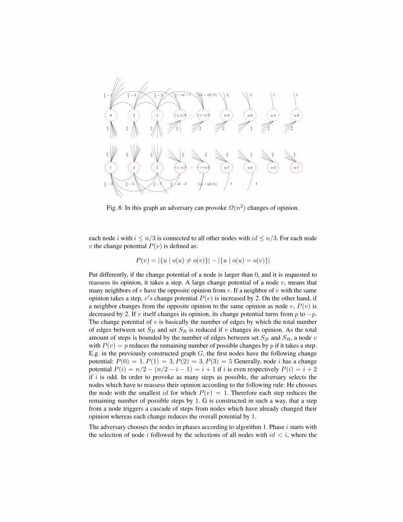
Fig. 8: In this graph an adversary can provoke Ω(n2) changes of opinion.

each node i with i ≤ n/3 is connected to all other nodes with id ≤ n/3. For each nodev the change potential P (v) is defined as:

P (v) = |u | o(u) 6= o(v)| − |u | o(u) = o(v)|

Put differently, if the change potential of a node is larger than 0, and it is requested toreassess its opinion, it takes a step. A large change potential of a node v, means thatmany neighbors of v have the opposite opinion from v. If a neighbor of v with the sameopinion takes a step, v′s change potential P (v) is increased by 2. On the other hand, ifa neighbor changes from the opposite opinion to the same opinion as node v, P (v) isdecreased by 2. If v itself changes its opinion, its change potential turns from p to −p.The change potential of v is basically the number of edges by which the total numberof edges between set SB and set SR is reduced if v changes its opinion. As the totalamount of steps is bounded by the number of edges between set SB and SR, a node vwith P (v) = p reduces the remaining number of possible changes by p if it takes a step.E.g. in the previously constructed graph G, the first nodes have the following changepotential: P (0) = 1, P (1) = 3, P (2) = 3, P (3) = 5 Generally, node i has a changepotential P (i) = n/2 − (n/2 − i − 1) = i + 1 if i is even respectively P (i) = i + 2if i is odd. In order to provoke as many steps as possible, the adversary selects thenodes which have to reassess their opinion according to the following rule: He choosesthe node with the smallest id for which P (v) = 1. Therefore each step reduces theremaining number of possible steps by 1. G is constructed in such a way, that a stepfrom a node triggers a cascade of steps from nodes which have already changed theiropinion whereas each change reduces the overall potential by 1.

The adversary chooses the nodes in phases according to algorithm 1. Phase i starts withthe selection of node i followed by the selections of all nodes with id < i, where the

adversary chooses the nodes in the reverse order than it did in round i − 1. Phase 0consists of node 0 changing its opinion, in phase 1 node 1 and then node 0 make steps,and in phase 2 the nodes change in the sequence 2, 0, 1. As a node v can only changeits opinion if P (v) > 0, we need to show that this is the case for each node v which isselected by the adversary. It is sufficient to show that each node which is selected has achange potential of 1.

We postulate:

(i) At the beginning of phase i, the following holds:P (i) = 1 and ∀v < i : o(v) = o(i).

(ii) Each node the adversary selects has change potential 1 and each node with id ≤ iis selected eventually in phase i.

(iii) At the end of phase i, all nodes with id ≤ i have opinion R if i is even and opinionB if i is odd.

We prove (i), (ii) and (iii) by induction. Initially, part (i) holds, as no node with id < 0exists and as node 0 is connected to n/2 nodes with opinion R and to n/2 − 1 nodeswith opinion B and therefore has change potential 1. In phase 0 only node 0 is selected,therefore part (ii) of holds as well. Node 0 changed its opinion and has therefore at theend of phase 0 opinion R, therefore part (iii) holds as well.

Now the induction step: To simplify the proof of part (i) of we consider odd and evenphases separately. Consider an odd phase i. At the start of phase i, no node with id ≥ ihas changed its opinion yet. Therefore node i still has its initial opinion o(i) = R.According to (iii), each node with id ≤ i − 1 has at the end of phase i − 1 opinionR = o(i). So (i + 1)/2 neighbors of i have compared to the initial state, changedtheir opinion from B to R. If a neighbor u of a node v with a different opinion thanv changes it, v′s change potential is decreased by 2. Therefore node i′s initial changepotential Pt0(i) = n/2− (n/2− i− 2) = i+ 2 is decreased by 2 · (i+ 1)/2 = i+ 1and is therefore P (i) = i + 2 − (i + 1) = 1 at the beginning of phase i. Therefore (i)holds before an odd phase.

Now consider an even phase i. At its start, all nodes with id ≥ i still have their initialopinion. Therefore node i has opinion o(i) = B. According to (iii) each node withid ≤ i − 1 has at the end of phase i − 1 opinion B = o(i). As node i′s initial changepotential was Pt0(i) = n/2 − (n/2 − i − 1) = i + 1 and i/2 neighbors of i changedfrom opinion R to opinion B compared to the initial state, i′s new change potential iscalculated as P (i) = i + 1 − 2 · i/2 = 1. Therefore (i) holds before an even phase,hence (i) holds.

To prove part (ii) let v be the last node which was selected in phase i − 1. As v wasselected, it had according to (ii) a change potential of 1. If a node changes its opinion,its change potential gets inversed. Therefore node v had at the beginning of phase ia change potential of −1. In addition, node v is by construction a neighbor of node iand has according to (i) at the start of phase i the same opinion as node i. As nodei changes its opinion, node v′s change potential is increased by 2. Therefore v′s newchange potential is again −1 + 2 = 1, when it is selected by the adversary. The sameargument holds for the second last selected node u. After it was selected in phase i− 1

its change potential was −1. Then v has changed its opinion which led to P (u) = −3.As node i and node v changed their opinions in phase i, P (u) was again 1. Hence ifthe adversary selects the nodes in the inverse sequence as in phase i− 1, each selectednode has a change potential of 1 and is selected eventually. Therefore (ii) holds.

As node i and all nodes with id ≤ i− 1 had at the beginning of phase i the opinion o(i)according to (iii) and all nodes have changed their opinion in phase i according to (ii),all nodes with id ≤ i must have the opposite opinion at the end of phase i, namely R ifi is even or B otherwise. Therefore (iii) holds as well.

We now have proven that in phase i, i nodes change their opinion. As the adversarystarts n/3 phases, the total number of steps is 1/2 · n/3 · (n/3− 1) ∈ Ω(n2). ut

Directly from Lemma 1 and Lemma 2, we get the following theorem.

Theorem 4. A worst case sequential IN reaches a fixed state after Θ(n2) steps.

We have seen, that with an adapted graph and an adversary an IN takes up to Θ(n2)steps until it stabilizes. But how bad can it get, if the process is benevolent instead?

Theorem 5. An IN with a benevolent sequential process reaches a fixed state afterΘ(n) steps.

Proof. A benevolent process needs Ω(n) steps to reach a stable state. This can be seenby considering the complete graphKn with initially bn/2c−1 red nodes and dn/2e+1blue nodes. Independently of the chosen sequence this IN needs exactly bn/2c−1 stepsto stabilize because the only achievable stable state is all nodes being blue. To proof thatthe number of steps is bounded by O(n) we define the following two sets: The set ofall red nodes which want to change: CRi = v | o(v) = R ∧ P (v) > 0 and the set ofall blue nodes which want to change: CB = v | o(v) = B ∧P (v) > 0. A benevolentprocess chooses nodes in two phases. In the first phase it chooses nodes from CB untilthe set is empty. During this phase, it may happen that additional nodes join CB (e.g. aleaf of a node v ∈ CB , after v made a step). However, no node which leftCB will rejoin,as those nodes turned red and can not turn blue again in this phase. In the second phase,the benevolent process chooses nodes from CR until this set is empty. The set CB willstay empty during the second phase since nodes turning blue can only reinforce bluenodes in their opinion. Both phases take at most n steps, therefore proving our upperbound. ut

References

[AAB+11] Yehuda Afek, Noga Alon, Omer Barad, Eran Hornstein, Naama Barkai, and ZivBar-Joseph. A biological solution to a fundamental distributed computing prob-lem. Science, 331:183–185, 2011.

[AG92] Frederick R. Adler and Deborah M. Gordon. Information collection and spread bynetworks of patrolling ants. The American Naturalist, 140:373–400, 1992.

[AG10] Arthur U. Asuncion and Michael T. Goodrich. Turning privacy leaks into floods:surreptitious discovery of social network friendships and other sensitive binaryattribute vectors. In Workshop on Privacy in the Electronic Society (WPES), pages21–30, 2010.

[ALP12] Chen Avin, Zvi Lotker, and Yvonne Anne Pignolet. On the elite of social networks.Personal communication, 2012.

[BP98] S. Brin and L. Page. The anatomy of a large-scale hypertextual web search engine.In Seventh International World-Wide Web Conference (WWW), 1998.

[BTZ+09] Danny Bickson, Yoav Tock, Argyris Zymnis, Stephen P. Boyd, and Danny Dolev.Distributed large scale network utility maximization. CoRR, abs/0901.2684, 2009.

[CYZ10] Wei Chen, Yifei Yuan, and Li Zhang. Scalable influence maximization in socialnetworks under the linear threshold model. In Industrial Conference on DataMining (ICDM), pages 88–97, 2010.

[DFF11] Benjamin Doerr, Mahmoud Fouz, and Tobias Friedrich. Social networks spreadrumors in sublogarithmic time. In Symposium on Theory of Computing (STOC),pages 21–30, 2011.

[FER91] Thomas M. J. Fruchterman, Edward, and Edward M. Reingold. Graph drawing byforce-directed placement. Software: Practice and experience, 21(11):1129–1164,1991.

[FKPS10] Patrik Floreen, Petteri Kaski, Valentin Polishchuk, and Jukka Suomela. Brief an-nouncement: distributed almost stable marriage. In Principles of Distributed Com-puting (PODC), pages 281–282, 2010.

[Gar70] Martin Gardner. Mathematical Games The fantastic combinations of John Con-way’s new solitaire game ”life”. Scientific American, 223:120–123, 1970.

[GO80] E. Goles and J. Olivos. Periodic behaviour of generalized threshold functions.Discrete Mathematics, 30(2):187 – 189, 1980.

[GS62] D. Gale and L. S. Shapley. College Admissions and the Stability of Marriage. TheAmerican Mathematical Monthly, 69:9–15, 1962.

[GT83] E. Goles and M. Tchuente. Iterative behaviour of generalized majority functions.Mathematical Social Sciences, 4:197 – 204, 1983.

[Hei46] F. Heider. Attitudes and cognitive organization. Journal of Psychology, 21:107–112, 1946.

[Hoe11] Martin Hoefer. Local matching dynamics in social networks. In InternationalColloquium on Automata, Languages and Programming (ICALP), pages 113–124,2011.

[Kel58] H.C. Kelman. Compliance, identification, and internalization: Three processes ofattitude change. Journal of Conflict Resolution, 2:51–60, 1958.

[KK89] Tomihisa Kamada and Satoru Kawai. An algorithm for drawing general undirectedgraphs. Information Processing Letters, 31:7 – 15, 1989.

[KKT05] David Kempe, Jon M. Kleinberg, and Eva Tardos. Influential nodes in a diffusionmodel for social networks. In ICALP, pages 1127–1138, 2005.

[Kle99] Jon M. Kleinberg. Hubs, authorities, and communities. ACM Comput. Surv., 31,1999.

[Koh89] T. Kohonen. Self-organization and associative memory. Springer series in infor-mation sciences. Springer, 1989.

[KOW08] Jan Kostka, Yvonne Anne Oswald, and Roger Wattenhofer. Word of Mouth:Rumor Dissemination in Social Networks. In 15th International Colloquium onStructural Information and Communication Complexity (SIROCCO), June 2008.

[KPS10] Alexander Kipnis and Boaz Patt-Shamir. On the complexity of distributed stablematching with small messages. Distributed Computing, 23:151–161, 2010.

[KSSV00] R. Karp, C. Schindelhauer, S. Shenker, and B. Vocking. Randomized rumorspreading. In 41st Annual Symposium on Foundations of Computer Science(FOCS), 2000.

[KW01] M. Kaufmann and D. Wagner. Drawing graphs: methods and models. Lecturenotes in computer science. Springer, 2001.

[LHK10] Jure Leskovec, Daniel P. Huttenlocher, and Jon M. Kleinberg. Signed networksin social media. In Conference on Human Factors in Computing Systems (CHI),pages 1361–1370, 2010.

[LSK06] J. Leskovec, A. Singh, and J. Kleinberg. Patterns of influence in a recommendationnetwork. Advances in Knowledge Discovery and Data Mining, pages 380–389,2006.

[MMG+07] Alan Mislove, Massimiliano Marcon, Krishna P. Gummadi, Peter Druschel, andBobby Bhattacharjee. Measurement and analysis of online social networks. In 7thACM SIGCOMM conference on Internet measurement, pages 29–42, 2007.

[Neu66] John Von Neumann. Theory of Self-Reproducing Automata. University of IllinoisPress, 1966.

[NS92] K. Nagel and M. Schreckenberg. A cellular automaton model for freeway traffic.Journal de Physique I, 2:22212229, 1992.

[Pea82] J. Pearl. Reverend Bayes on inference engines: A distributed hierarchical ap-proach. In Second National Conference on Artificial Intelligence (AAAI), pages133–136, 1982.

[PS83] Svatopluk Poljak and Miroslav Sra. On periodical behaviour in societies withsymmetric influences. Combinatorica, 3:119–121, 1983.

[RT98] Edmund T. Rolls and Alessandro Treves. Neural Networks and Brain Function.Oxford University Press, USA, 1 edition, 1998.

[SS10] Thomas Sauerwald and Dirk Sudholt. A self-stabilizing algorithm for cut prob-lems in synchronous networks. Theor. Comput. Sci., 411:1599–1612, 2010.

[SS11] Thomas Sauerwald and Alexandre Stauffer. Rumor spreading and vertex expan-sion on regular graphs. In Symposium on Discrete Algorithms (SODA), pages462–475, 2011.

[Wat02] Duncan J. Watts. A simple model of global cascades on random networks. Pro-ceedings of the National Academy of Sciences, 99:5766, 2002.

[Win08] Peter Winkler. Puzzled: Delightful graph theory. Communications of the ACM,51:104–104, 2008.

[Wol02] Stephen Wolfram. A New Kind of Science. Wolfram Media, 1 edition, 2002.

Appendix

A Synchronous IN

A.1 Transistor

In this section, we formally define how a transistor must be connected to the rest of the graph andhow it behaves in that case. The symbol T is used to denote a particular graph as well as instancesof that graph, which are induced subgraphs; the symbols C(T ), E(T ),Bx(T ) are used to denotethe respective vertex sets of an instance T . In order to talk about how a transistor should fit in anetwork, we introduce the outside influence function, which specifies how an induced subgraphis influenced by the rest of the graph.

Definition 3. For any vertex v ∈ V H , where H = (V H , EH) is an induced subgraph ofG = (V,E), the outside influence at time t exerted on said vertex is equal to the following:IHt (v) = o0(v) ·

∑u∈u′|v,u′∈E\EH ot(u).

So if IHt (v) is positive, node v will be influenced by the rest of the graph to stick with its initialopinion or change back to it; if IHt (v) is negative, v will be influenced to change away from itsinitial opinion. The upper right indices are sometimes left out if they are clear from the context.We are now able to formally specify an outside influence range in which the transistor will operatecorrectly.

Definition 4. An instance T = (V T , ET ) of a transistor T (k) with k ≥ 1 and with outsideinfluence ITt (·) is correctly accessed with initial opinionX if and only if the following conditionshold.

(i) o0(v) = X for all v ∈ V T

(ii) It(v) = −k for all t and all v ∈ C(T )(iii) |It(v) |≤ k − 1 for all t and all v ∈ E(T )(iv) It(B1(T )) ∈ −3,−1, 1 for all t(v) It(B2(T )) = −1 for all t

(vi) It(B3(T )) = −(k + 1) for all t

Note that if all collector edges in Figure 1 advertise R then the conditions (ii) through (vi) arefulfilled independent of that the other edges connecting the transistor to the rest of graph advertise.Because of (ii) there is a strong outside influence on the collector vertices to change their opinion.The first round t where It(B1(T )) is equal to −3 (both base edges in Figure 1 advertise R), willcause that eventually all vertices in the transistor flip their opinion to (−X). We call this event tflip time tf (T ) of T .

Lemma 3. If an instance T = (V T , ET ) of a transistor T (k) is correctly accessed with initialopinion X , then the following statements hold.

(i) All vertices v ∈ V T are of opinion ot(v) = X for all t ≤ tf (T )

(ii) All vertices v ∈ E(T ) are of opinion ot(v) = X for all tf (T ) < t ≤ tf (T ) + 3

(iii) All vertices v ∈ V T are of opinion ot(v) = (−X) for all t ≥ tf (T ) + 4

Proof. First note that the vertices in E(T ) can not change their opinion until at least one in C(T )has done so since they each have an outside influence of at most (k − 1) times (−X) after (iii)of definition 4 and an inside influence of k times X from the k vertices in C(T ). Similarly, thevertices in C(T ) can not change their opinion until B3(T ) and B2(T ) have done so and theyin turn have to wait for B1(T ) to change. Finally, B1(T ) will only change after the flip timetf (T ). This takes care of (i) and (ii). To see that (iii) is true note that after the flip event the sets(B1(T ), B2(T ),B3(T ), C(T ), E(T )) will indeed all change their opinion in the given orderand that even if after the flip event the outside influence of B1(T ) will go back to some number> −3, the process can still not be stopped or reversed. ut

A.2 Counters

The final graph for our intended lower bound is a recursively defined counter. In this section, wepresent the base case in form of a simple 2-Path graph as well as the recursive case. In the latter,a counter is combined with a number of transistors to form a bigger counter as suggested in theproof outline.

A counter K = (H = (V,E), I(·),RR,RB ,S(·)) consists of a graph H = (V,E), a func-tion I : V → Z, specifies the valid range of outside influence, two special interest verticesRR,RB ∈ V , which indicate when the graph has finished running, and an initial configurationS(·).We will postpone the definition of the axioms a counter must satisfy, and first describe how acounter is properly connected and accessed since the behavior of a counter need only be definedif it is connected and accessed correctly.

Definition 5. A counter K = (H = (V H , EH), I(·),RR,RB ,S(·)) is correctly accessed andcorrectly initialized from t1 to t2 if and only if the following condition holds.

(i) For all v in V H the initial state of v is set by ot1(v) = S(v).(ii) For all X and all t1 ≤ t ≤ t2 the outside influence is given by IHt (v) = I(v)

A counter is considered reversely initialized if (i) is changed to ot1(v) = −S(v), and it isconsidered reversely accessed if (ii) is changed to −I(v) = IHt (v). We sometimes add thekeyword virtually to indicate some deviations from the definition which do not result in an alteredbehavior of H .

Definition 6. A tuple K = (H = (V H , EH), I(·),RR,RR,S(·)) is a proper counter withconvergence time c and supply edge number e if and only if correct access and correct initializa-tion from t1 to t2 imply that the following statements hold.

(i) e =∑v∈V K |I(v)·S(v)>0 I(v) · S(v) =

∑v∈V K |I(v)·S(v)<0−I(v) · S(v)

(ii) d√e+ 2e+ 1 ≥ maxv∈V K |I(v)|

(iii) The verticesRX are of opinion X for all t ≤ mint1 + c− 1, t2 + 1(iv) For all vertices v ∈ V H and all t1 + c ≤ t ≤ t2 +1 the following is true ot(v) = −ot1(v).

The edge supply number corresponds to the number of black edges in Figure 2 and (i) satisfied ifit is the same for blue and red. We will need condition (ii) to make sure that we do not producea multigraph, (iii) indicates thatRX only change their opinion after l rounds when the graph hasfinished running, and (iv) makes it possible to run the counter again with reverse opinions. Notethat if a counter is correctly initialized and reversely accessed, or if it is reversely initialized andcorrectly accessed from t1 to t2, ot(v) will be time-constant from t1 to t2 because of (iv).

2-Path graph The 2-Path graph counter will be the base case of our final, recursively definedgraph. It consists just of two simple paths one of which is initialized withR and the other withB.If accessed correctly, the following will happen on both paths simultaneously. All vertices willchange their opinion in the order in which they occur on their respective paths.

Definition 7. A 2-Path graph is defined as P2(l) = (H = (V H , EH), I(·),RR,RB ,S(·))where

V H = vRi | 0 ≤ i < l ∪ vBi | 0 ≤ i < l

EH = vRi , vRi+1 | 0 ≤ i < l − 1 ∪ vBi , vBi+1 | 0 ≤ i < l − 1

I(v) =

−2 if v = vX0

−1 if v ∈ vXi | 1 ≤ i < l − 10 otherwise

RX = vXl−1

S(vXi ) = X

Lemma 4. A 2-Path graph P2(l) is a valid counter with n = 2l vertices, convergence time c = land supply edge number e = l.

Proof. We will have to prove the conditions in definition 6 under the assumption that the condi-tion in the definition 5.

The conditions (i) and (ii) are trivially true. For (iii) note that from condition (ii) of definition 5and the definition of I(·), it follows that the vertices in vXi | 1 ≤ i < l − 1 all have one moreoutside neighbor of the opinion −X than of the opinion X, the vertices vX0 has two more outsideneighbors of the opinion (−X) than of the opinion X, and vXl−1 has the same number of outsideneighbors of the opinion (−X) as of the opinion X . This means that the vertices vX0 will changeits opinion to (−X) in the first round, and cause vX1 to turn in the second and so forth. In otherwords, ot(vXi ) will be X for all t ≤ i and (−X) ever after. Therefore, ot(RX) = ot(v

Xl−1) is

equal to X for all t ≤ l − 1, and condition (iii) of definition 6 is satisfied.

Also note that at time l all vertices will have turned and are not going to reverse back to theiroriginal position therefore satisfying condition (iv). ut

Repeater A repeater is a function that takes a counter and uses transistors to repeatedly run thatcounter and so produce a counter with much higher convergence time at the expense of an onlyslightly increased number of vertices. However in addition to what was suggested in section 4 weneed two new verticesRR,RB to indicate when the graph has reached a stable state as displayedin Figure 9. On first reading, the reader is advised to have a look at the definition of a repeaterand the content of the Lemmas 6 and 9, and then skip to section A.3.

TR1

vR vBv3BvR3 v2

BvR2 v1R v1

Bv0Bv0

R

T1B

TR2 T0

R

T0B T2

B

C(4)

Fig. 9: Full repeater graph R(1, P2(4)) with a P2(4) as graph which is repeatedly runand six transistors to run P2(4) three times.

Definition 8. A repeater is a function R which when it is given a number j and a counterK = (H = (V H , EH), I(·), RR, RB , S(·)) with convergence time c, n vertices, and supply

edge number e, produces a tuple R(K, j) = (H = (V H , EH), I(·),RR,RB ,S(·)) where

TXi = (V X

i , EXi ) for 0 ≤ i ≤ 2j,X ∈ R,B are instances of transistors T (s)

V H =

j−1⋃X∈R,B,i=0

V Xi

∪ V H ∪ vR ∪ vB

EH =

j−1⋃X∈R,B,i=0

EXi

∪ EH ∪ E1 ∪ E2 ∪ E3 ∪ E4 ∪ E5

E1 = RX ,B1(T−X2i ) | 0 ≤ i ≤ 2j ∪ RX ,B1(TX

2i+1) | 0 ≤ i ≤ 2j − 1 (green in Figure 9)

E2 = RX ,RX|X ∈ R,B (orange in Figure 9)

I(v) =

−2 if v = B1(TX0 )

−1 if v = B1(TXi ) for some 1 ≤ i ≤ 2j

−1 if v = B2(TXi ) for some 0 ≤ i ≤ 2j

−(s+ 1) if v = B3(TXi ) for some 0 ≤ i ≤ 2j

−s if v ∈ E(TXi )

1 if v = RX

−1 if v = RX

0 otherwise

RR = vR

RB = vB

S(v) =

S(v) if v ∈ V T

X if v ∈ V Xi

X if v = RX

s = d√e+ 2e+ 1

E3 (black in Figure 9) consists the following edges. For every vertex v ∈ V H with k = |I(v)|and with X = sign(I(v)S(v)), there are edges from v to k different emitter vertices of everyT−X2i with 0 ≤ i ≤ j and of every TX

2i+1 with 0 ≤ i ≤ j − 1 .

E4 (magenta in Figure 9) consists of the following edges. For every 0 ≥ i ≥ 2j−1 andX , thereis an edge from B1(TX

i+1) to an emitter vertex of TXi and there is one edge from an emitter vertex

of TX2j toRX .

E5 (cyan in Figure 9) consists of the following edges. For all X , there is an edge from RX to anemitter vertex of every TX

2i with 0 ≤ i ≤ j and of every T−X2i+1 with 0 ≤ i ≤ j − 1.

Lemma 5. The repeater R(K, j) does indeed exist such that the emitter vertices of Ti are con-nected to no more than (s− 1) vertices outside Ti.

Proof. We have to show that there are E3, E4 and E5 such that the emitter vertices of thetransistors do not have too many outside edges. Every transistor’s emitter vertices have e edgesleaving the transistor in E3 because of condition (i) of definition 5, one edge in E4 and one edgein E5. This is a total of e+ 2 necessary edges. A transistor T (s) has s collector vertices each ofwhich should have no more than (s− 1) outside edges where s = d

√e+ 2e+ 1. This makes a

total of more than possible e+ 2 edges.

s(s− 1) = (d√e+ 2e+ 1)(d

√e+ 2e+ 1− 1)

> d√e+ 2e2

≥ e+ 2

Additionally condition (ii) of definition 5 shows that |I(v)| ≤ s. This is necessary because wecould otherwise only realize the graph if we were allowed multigraphs. ut

Lemma 6. The repeater R(K, j) has n = 2(2j +1)(2s+1)+ n+2 vertices and supply edgenumber e = (2j + 1)(s2 + s+ 3) + 3 where s = d

√e+ 2e+ 1.

Proof. To obtain the number of vertices we add the number of vertices in a transistor times thenumber of transistors to the number in the counter K and two verticesRX .

|V H | = 2(2j + 1)|T (s)|+ |V H |+ 2

= 2(2j + 1)(2s+ 3) + n+ 2

To obtain the supply edge number we just the go through the cases in the definition of S(·) andadd them up.

e = 1 · 2 + 2j · 1 + (2j + 1) · 1 + (2j + 1) · (s+ 1) + (2j + 1)s · s+ 1 · 1 + 1 · 1

= 2(2j + 1) + (2j + 1)(s+ 1) + (2j + 1)s2 + 3

= (2j + 1)(s2 + s+ 3) + 3

ut

Lemma 7. For all 0 ≤ i ≤ 2j and all X , TXi is accessed correctly.

Proof. Condition (i) of definition 4 is trivially true. The collector vertices as well as B2 andB3 of Ti have no edges to other parts of H so it holds that ITi

t (v) = IHt (v) = I(v) for allv ∈ C(Ti) ∪ B2(Ti) ∪ B3(Ti). Therefore, (ii),(v) and (vi) are fulfilled.

Condition (iii) of is fulfilled because of Lemma 5.

For condition (iv) we distinguish between i = 0 and i 6= 0. If i is equal to 0, then B1(TXi ) has 1

edge coming from outside V Xi but still insideH and an outside influence of IH(B1(TX

i )) = −2.If i is not equal to 0, then B1(TX

i ) has 2 edges coming from outside V Xi but still insideH and an

outside influence of IH(B1(TXi )) = −1. In both cases, the resulting IT

Xi (B1(TX

i )) will satisfy(iv). ut

Lemma 8. The transistors flip in order. That is, the following statements must hold.

(i) If tf (TXi ) = t there must be a t′ ≤ t− 4 such that tf (TX

i−1) = t′ for all 1 ≤ i ≤ 2j.(ii) If OR

X

t (RX) = −X there must be a t′ ≤ t− 4 such that tf (TX2j ) = t′

Proof. The vertexRX has total influence Ivt (RX) = IHt (RX) + ot(RX) + ot(E(TX2j )) which

is equal to 1 + X · (ot(RX) + ot(E(TX2j ))). So RX can only change its opinion to (−X)

if both ot(RX) and ot(E(TX2j )) are (−X). Similarly IT

Xi

t (B(TXi )) which can be written as

IHt (B(TXi )) +X(ot(E(TX

i−1)) + ot(R)) = −1 +X(ot(E(TXi−1)) + ot(R)) can only be −3 if

E(TXi−1) is −X for all 1 ≤ i ≤ 2j. This together with statements (i) and (ii) of Lemma 3 we get

the required statements. ut

Definition 9. We define 1IH(·), 2IH(·), 3IH(·) and 5IH(·) to be the outside influence exertedon vertices in H by E1, E2, E3 and E5 respectively.

Note that IHt (v) = 1IHt (v) + 2IHt (v) + 3IHt (v) + 5IHt (v) + IHt (v). The edges E4 are inten-tionally left out since they do not have endpoints in H .

Lemma 9. R(j, K) is indeed a counter of convergence time c = (2j + 1)(c+ 4) + 1.

Proof. So assume that the constant outside influence of all vertices is given by IH(·) = IH(·).We define c to be the smallest t with ot(RR) = B or ot(RB) = R. By Lemma 8 all transistorshave flipped at time c. For all t < c and all vertices v ∈ H , the outside influences of 2IHt (v) andof IHt (v) cancel out each other so we need only care about 1IH(), 3IH() and 5IH() until wereach time c.

To get a induction hypothesis we prove the following stronger statement: tf (T 2l) = 2l(c + 4)and o2l(c+4)(v) = S(v) for all 0 ≤ l ≤ j and for all vertices v in H .

The base case for l = 0 is trivial. For the induction step l → l + 1 assume tf (T 2l) = 2l(c+ 4)and o2l(v) = S(v) is true for all vertices v in H . We will in the following look at how the graphbehaves in the following intervals [2l(c+4), 2l(c+4)+3], [2l(c+4)+4, (2l+1)(c+4)− 1],[(2l+1)(c+4), (2l+1)(c+4)+3] and [(2l+1)(c+4)+4, (2l+2)(c+4)−1]. I.e., we takethe behavior during the interval [a, b] to mean the influences exerted in [a, b] and their outcomesin [a+ 1, b+ 1].

Interval [2l(c+ 4), 2l(c+ 4) + 3]. We will show that K is correctly initialized and virtuallyreversely accessed from 2l(c+4) to 2l(c+4)+3. Therefore and because of (iii) in definition 6,o2l(c+4)+4(·) will still be equal to S(·).

Let us start by considering 1IH(·) + 5IH(·). Using Lemma 8 we can deduce the followingstatement. All transistors TX

i with i < 2l have already switched completely by 2l(c + 4) (theyare in the region specified by (iii) of Lemma 3, similarly all such transistors with i > 2l can onlystart switching after i(c + 4) + 3 (they are in the region specified by (i) of Lemma 3. So thecontribution of TY

i to 1IH() is canceled out by the contribution of T−Yi to 5IH() for all i 6= 2l

and vice versa. And for TX2l we know that oi(E(TX

2j )) = X for i ≤ 2l(c4) + 3 from (i), (ii)of Lemma 3. Therefore, 1IHi (v) + 5IHi (v) must be non-negative for RX and zero for all othervertices.3IHi (·) will be exactly −I(·) for 2l(c + 4) ≤ i ≤ 2l(c + 4) + 3 because the transistors TY

i

with an even i 6= 2l cancel out each other and those with i = 2l will have ot(E(TXi )) = X

for t ≤ 2l(c+ 4) + 3 so TXi will exactly contribute the required outside influence of −I(·). So

ITt (v) = 1IHt (v) + 3IHt (v) + 5IHt (v) will be −I(v) for all v except forRR andRB . HoweverRX is supposed to stick with o(RX) = X , in case of correct initialization and reverse accessand the deviation introduced by 1IH() + 5IH() further encourages them to do so. Therefore Kis a correctly initialized and virtually reversely accessed counter.

Interval [2l(c + 4) + 4, (2l + 1)(c + 4) − 1]. We will use a proof of induction over kto show that K is accessed and initialized correctly from 2l(c + 4) + 4 to 2l(c + 4) + 4 + kand that tf (TX

2l+1) ≥ 2l(c + 4) + k for all k < c. Using (iv) of definition 6 the inductionstatement for k set to c− 1 will imply that o(2l+1)(c+4)(·) = −S(·). This in turn will imply thattf (TX

2l+1) = (2l + 1)(c+ 4).

Because of Lemma 8 and because o2l(c+4)(RX) = X , tf (T e2l+1) must be bigger than 2l(c+4)+4.

Therefore, of all transistors each one will be of uniform opinion at 2l(c + 4), and therefore1IH2l+4() +

5IH2l+4() will be 0. 3IH2l+4(v) will be exactly I(v). This is because for the same rea-son as in the previous interval all transistors TX

i with i 6= 2l cancel out the transistors i = 2l havealready flipped completely. Hence, K is accessed and initialized correctly from 2l(c+ 4) + 4 to2l(c+ 4) + 4. This covers the base case of our induction.

Now assuming K is accessed and initialized correctly from 2l(c+ 4) + 4 to 2l(c+ 4) + 4 + kand tf (TX

2l+1) ≥ 2l(c + 4) + k for some k < c. Because of the first assumption and becausek + 1 < c we can apply (iii) of definition 6. Hence o2l(c+4)+k(RX) = X will still be true andas a direct consequence tf (TX

2l+1) ≥ 2l(c+ 4) + k + 1 and we have proven the first part of ourinduction statement. Now since tf (TX

2l+1) ≥ 2l(c + 4) + k + 1 TX2l+1 is still uniformly of the

opinion X at 2l(c+4)+ k+1, so IH2l(c+4)+k+1(·) is still equal to I(·). This also means that Kis still correctly accessed and therefore proves our induction statement.

Interval [(2l + 1)(c + 4), (2l + 1)(c + 4) + 3] The graph K is reversely initialized andvirtually correctly accessed from (2l+ 1)(c+ 4) to (2l+ 1)(c+ 4) + 3. We know from the lastinterval that K is reversely initialized and that TX

(2l+1) = (2l + 1)(c + 4) The proof of correctaccess is completely analogous to the first interval. Therefore and because of (iii) in definition 6,o2l(c+4)+4(·) will still be equal to −S(·).

Interval [(2l+ 1)(c+ 4) + 4, (2l+ 2)(c+ 4)− 1] The graph K is accessed and initializedreversely from (2l+1)(c+4)+ 4 to (2l+2)(c+4)− 1 and tf (TX

2l+2) = 2l(c+4). We knowfrom the last interval that K is reversely initialized the rest of the proof is completely analogousto the second interval. Therefore o(2l+2)(c+4)(·) = S(·).This concludes the proof of the induction step. Now we only need to show that we can indeedderive the Lemma from this induction result. At time 2j(c+ 4) we basically have the same caseas at the beginning of the first interval and using the same technique as in the first and secondinterval we can deduce that the first time t with IHt (RX) < 0 is (2j+1)(c+4) (this proves (iii)of definition 6). We can in the same manner prove that o(2j+1)(c+4)(v) = −S(v) for all v ∈ V H .And since all transistors have already flipped completely and because K is reversely initializedand correctly accessed from (2j+1)(c+4) to infinity (iv) is also fulfilled. The conditions (i) aretrue because of Lemma 6 and finally (ii) is true since

d√e+ 2e+ 1 = d

√(2j + 1)(s2 + s+ 3) + 3 + 2e+ 1

≥ d√s2e+ 1

= s+ 1

= maxv∈V H

I(v).

ut

A.3 Putting it all together

Lemma 10. For every l ≥ 1 and h ≥ 0, there is a counter K with n ≤ (h + 1)54(1 + 80√

l

)hl

vertices, supply edge number e ≤ l2−12h ·

(1 + 80√

l

)hand convergence time c ≥ l2−

12h .

Proof. We prove this by induction over h. For h = 0K is trivially given by P2(l). Now given a

counter K with n ≤ (h + 1)54(1 + 80√

l

)hl vertices, convergence time c ≥ l

2− 12h and supply

edge number e ≤ l2− 1

2h ·(1 + 80√

l

)hwe construct K = R(K, 1

2bl

12h+1 c). By Lemma 9 the

convergence time c is at least (2 12bl

12h+1 c + 1)(l

2− 12h + 4) which is in turn at least l2−

12h+1 .

To prove the bound on the supply edge number, we first show a bound for the transistor size s byusing the definition of R. The required bound for the supply edge number of K can be deducedusing Lemma 6.

s = d√e+ 2e+ 1 (1)

≤

√l2− 1

2h ·(1 +

80√l

)h

+ 2 + 2 (2)

≤

√(1 +

2

l

)l2− 1

2h ·(1 +

80√l

)h

+ 2 (3)

≤(1 +

2

l

)√l2− 1

2h ·(1 +

80√l

)h

+ 2 (4)

≤(1 +

2

l+

2√l

)√l2− 1

2h ·(1 +

80√l

)h

(5)

≤(1 +

4√l

)√l2− 1

2h ·(1 +

80√l

)h

(6)

e = (2j + 1)(s2 + s+ 3) + 3 where j =1

2bl

12h+1 c

≤(1 +

1

l

)· l

12h+1 (s2 + s+ 3) + 3

≤(1 +

1

l

)· l

12h+1

((s+

1

2

)2

+11

4

)+ 3

≤(1 +

1

l

)· l

12h+1

(1 + 4√l

)√l2− 1

2h ·(1 +

80√l

)h

+1

2

2

+11

4

+ 3

≤(1 +

1

l

)· l

12h+1

(1 + 5√l

)√l2− 1

2h ·(1 +

80√l

)h2

+11

4

+ 3

≤(1 +

1

l

)· l

12h+1

((1 +

10√l+

25

l

)l2− 1

2h ·(1 +

80√l

)h

+11

4

)+ 3

≤(1 +

1

l

)· l

12h+1

(1 +

38√l

)l2− 1

2h ·(1 +

80√l

)h

+ 3

≤(1 +

77√l

)· l2−

12h+1 ·

(1 +

80√l

)h

+ 3

=

(1 +

80√l

)h+1

l2− 1

2h+1

When contracting terms in (3) and (5), we use the fact that l2−12h ≥ l and

(1 + 80√

l

)h≥ 1.

Using the same lemma, also gives the needed bound for the number of vertices n.

n = 2(2j + 1)(2s+ 3) + n+ 2 where n = (h+ 1)54

(1 +

80√l

)h

l

≤ 2

(1 +

1

l

)l

12h+1 (2s+ 3) + n+ 2

≤(2 +

2

l

)l

12h+1

2

(1 +

4√l

)√l2− 1

2h ·(1 +

80√l

)h

+ 3

+ n+ 2

≤(2 +

2

l

)l

12h+1

(2 +

11√l

)√l2− 1

2h ·(1 +

80√l

)h

+ n+ 2

≤(4 +

48√l

)l

12h+1 · l1−

12h+1

(1 +

80√l

)h2

+ n+ 2

≤(4 +

50√l

)(1 +

80√l

)h2

l + n

≤ 54

(1 +

80√l

)h2

l + (h+ 1)54

(1 +

80√l

)h

l

≤ (h+ 2)54

(1 +

80√l

)h

l

≤ (h+ 2)54

(1 +

80√l

)h+1

l

ut

We need one more additional tool from mathematics to proof our final Theorem 3.

Lemma 11. For every x > 0 and all n > 0 the following inequality holds(1 + x

n

)n ≤ ex

Proof. It is well known that the sequence sn(x) =(1 + x

n

)n converges to ex as n goes toinfinity. So we need only proof that sn(x) is non-decreasing in n. We achieve this by showing that

all coefficients in the power series sn(x) =∑∞

k=0 cknx

k =∑∞

k=0

(nk

)(xn

)k are non decreasing.

ckn+1

ckn=

(n+1k

)1

(n+1)k(nk

)1nk

(7)

=

(n+1)!k!(n+1−k)!

1(n+1)k

n!k!(n−k)!

1nk

(8)

=

1n+1−k

1(n+1)k−1

1nk

(9)

=nk

(n+ 1)k−1(n− (k − 1))(10)

≥ nk

nk(11)

= 1 (12)

In (10), the arithmetic mean of the factors in the denominator (numerator respectively) is n.Since the geometric mean of positive numbers can never be bigger than the arithmetic mean, thegeometric mean of the factors of the denominator has to be (≤ n) and the product (≤ nk). ut

Now we combine Lemma 10 and Lemma 11 to proof Theorem 3.

Proof. If we select h in Lemma 10 to be blog log lc we can get a counter with the followingdimensions for every l.

n ≤ (blog log lc+ 1)54

(1 +

80√l

)blog log lc

l (13)

≤ 108 log log l

(1 +

80

b√lc

)blog log lc

l (14)

≤ 108 log log l

(1 +

80

b√lc

)b√lc

l (15)

≤ 108 · e80 log log l · l (16)

e ≤ l2 · l−1

2blog log lc ·(1 +

80√l

)blog log lc

(17)

≤ l2 · l−1

log l · e80 (18)

=1

2l2 · e80 (19)

c ≥ l2 · l−1

2blog log lc (20)

≥ l2 · l−1

2(log log l)−1 (21)

= l2 · l−2

log l (22)

= l2 ·(l− 1

log l

)2(23)

=

(1

2

)2

l2 (24)

=1

4l2 (25)

(16) and (18) are true because of Lemma 11, and (19) and (24) are true because it holds thatlog(l− 1

log l

)= − 1

log llog l = −1 = log 1

2. We can also run this counter by creating a red and

a blue clique of size d√ee + 1 and then connecting the vertices in the counter to vertices in the

cliques according to I(·). Since√e = O(n) this increases the number of vertices only by a

constant fraction. So our final network has n = O(l · log log l) vertices and a convergence time

of Ω(l2) = Ω(

n2

(log log l)2

)≥ Ω

(n2

(log logn)2

). ut