Convergence Diagnostics - Patrick Lampatricklam.org/teaching/convergence_print.pdfAnother way to...

Convergence Diagnostics

Patrick Lam

Outline

Convergence

Visual Inspection

Gelman and Rubin Diagnostic

Geweke Diagnostic

Raftery and Lewis Diagnostic

Heidelberg and Welch Diagnostic

Running Example

As a running example, we will use the bivariate normal Metropolissampler from class.

> NormalMHExample <- function(n.sim, n.burnin) {

+ library(mvtnorm)

+ mu.vector <- c(3, 1)

+ variance.matrix <- cbind(c(1, -0.5), c(-0.5, 2))

+ theta.mh <- matrix(NA, nrow = n.sim, ncol = 2)

+ theta.current <- rnorm(n = 2, mean = 0, sd = 4)

+ theta.update <- function(index, theta.current, ...) {

+ theta.star <- rnorm(n = 1, mean = theta.current[index], sd = 2)

+ if (index == 1)

+ theta.temp <- c(theta.star, theta.current[2])

+ else theta.temp <- c(theta.current[1], theta.star)

+ r <- dmvnorm(theta.temp, mu.vector, variance.matrix)/dmvnorm(theta.current,

+ mu.vector, variance.matrix)

+ r <- min(r, 1, na.rm = T)

+ if (runif(1) < r)

+ theta.star

+ else theta.current[index]

+ }

+ for (i in 1:n.sim) {

+ theta.current[1] <- theta.mh[i, 1] <- theta.update(1, theta.current,


+ theta.current[2] <- theta.mh[i, 2] <- theta.update(2, theta.current,


+ }

+ theta.mh <- theta.mh[(n.burnin + 1):n.sim, ]

+ }

> mh.draws <- NormalMHExample(n.sim = 5000, n.burnin = 0)

Convergence

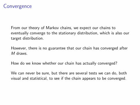
From our theory of Markov chains, we expect our chains toeventually converge to the stationary distribution, which is also ourtarget distribution.

However, there is no guarantee that our chain has converged afterM draws.

How do we know whether our chain has actually converged?

We can never be sure, but there are several tests we can do, bothvisual and statistical, to see if the chain appears to be converged.

Convergence Diagnostics in R

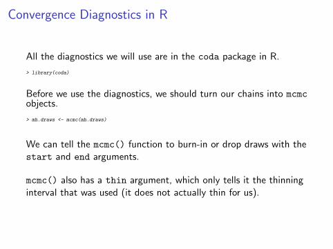
All the diagnostics we will use are in the coda package in R.

> library(coda)

Before we use the diagnostics, we should turn our chains into mcmcobjects.

> mh.draws <- mcmc(mh.draws)

We can tell the mcmc() function to burn-in or drop draws with thestart and end arguments.

mcmc() also has a thin argument, which only tells it the thinninginterval that was used (it does not actually thin for us).

Posterior Summary

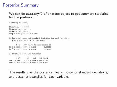
We can do summary() of an mcmc object to get summary statisticsfor the posterior.

> summary(mh.draws)

Iterations = 1:5000

Thinning interval = 1

Number of chains = 1

Sample size per chain = 5000

1. Empirical mean and standard deviation for each variable,

plus standard error of the mean:

Mean SD Naive SE Time-series SE

[1,] 3.0282 1.027 0.01453 0.03859

[2,] 0.9997 1.424 0.02014 0.04109

2. Quantiles for each variable:

2.5% 25% 50% 75% 97.5%

var1 0.864 2.37214 3.0489 3.733 5.016

var2 -1.622 0.03447 0.9984 1.927 3.777

The results give the posterior means, posterior standard deviations,and posterior quantiles for each variable.

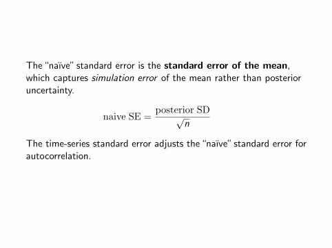
The“naıve” standard error is the standard error of the mean,which captures simulation error of the mean rather than posterioruncertainty.

naive SE =posterior SD√

n

The time-series standard error adjusts the“naıve”standard error forautocorrelation.

Outline

Convergence

Visual Inspection


Geweke Diagnostic



Mixing

One way to see if our chain has converged is to see how well ourchain is mixing, or moving around the parameter space.

If our chain is taking a long time to move around the parameterspace, then it will take longer to converge.

We can see how well our chain is mixing through visual inspection.

We need to do the inspections for every parameter.

TraceplotsA traceplot is a plot of the iteration number against the value ofthe draw of the parameter at each iteration.

We can see whether our chain gets stuck in certain areas of theparameter space, which indicates bad mixing.

0 2000 4000 6000 8000 10000

−2

02

4

Good Mixing

iteration

θθ

0 2000 4000 6000 8000 10000

0.5

1.0

1.5

2.0

2.5

3.0

3.5

Bad Mixing

iteration

θθ

Traceplots and Density Plots

We can do traceplots and density plots by plotting an mcmc objector by calling the traceplot() and densplot() functions.

> plot(mh.draws)

0 1000 3000 5000

01

23

45

6

Iterations

Trace of var1

0 2 4 6

0.0

0.1

0.2

0.3

N = 5000 Bandwidth = 0.196

Density of var1

0 1000 3000 5000

−4

02

46

8

Iterations

Trace of var2

−5 0 5 10

0.00

0.10

0.20

0.30

N = 5000 Bandwidth = 0.2726

Density of var2

Running Mean PlotsWe can also use running mean plots to check how well our chainsare mixing.

A running mean plot is a plot of the iterations against the mean ofthe draws up to each iteration.

0 2000 4000 6000 8000 10000

0.8

1.0

1.2

1.4

Good Mixing

Iteration

Mea

n

0 2000 4000 6000 8000 10000

1.4

1.5

1.6

1.7

1.8

1.9

2.0

Bad Mixing

Iteration

Mea

n

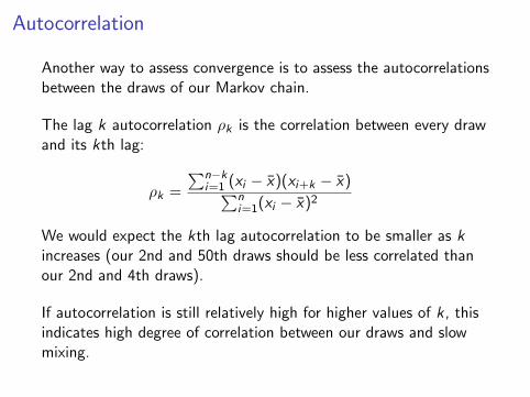
Autocorrelation

Another way to assess convergence is to assess the autocorrelationsbetween the draws of our Markov chain.

The lag k autocorrelation ρk is the correlation between every drawand its kth lag:

ρk =

∑n−ki=1 (xi − x)(xi+k − x)∑n

i=1(xi − x)2

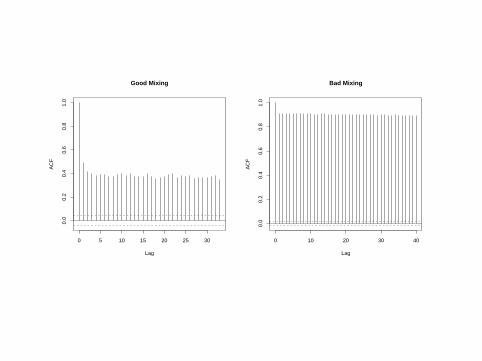
We would expect the kth lag autocorrelation to be smaller as kincreases (our 2nd and 50th draws should be less correlated thanour 2nd and 4th draws).

If autocorrelation is still relatively high for higher values of k, thisindicates high degree of correlation between our draws and slowmixing.

0 5 10 15 20 25 30

0.0

0.2

0.4

0.6

0.8

1.0

Lag

AC

F

Good Mixing

0 10 20 30 40

0.0

0.2

0.4

0.6

0.8

1.0

LagA

CF

Bad Mixing

Autocorrelation Plots

We can get autocorrelation plots using the autocorr.plot()function.

> autocorr.plot(mh.draws)

0 5 15 25

−1.

0−

0.5

0.0

0.5

1.0

Lag

Aut

ocor

rela

tion

0 5 15 25

−1.

0−

0.5

0.0

0.5

1.0

Lag

Aut

ocor

rela

tion

Rejection Rate for Metropolis-Hastings Algorithm

We can also get a rejection rate for the Metropolis-Hastingsalgorithm using the rejectionRate() function.

> rejectionRate(mh.draws)

var1 var2

0.5277055 0.4094819

To get the acceptance rate, we just want 1− rejection rate.

> acceptance.rate <- 1 - rejectionRate(mh.draws)

> acceptance.rate

var1 var2

0.4722945 0.5905181

Outline

Convergence

Visual Inspection


Geweke Diagnostic



Gelman and Rubin Multiple Sequence Diagnostic

Steps (for each parameter):

1. Run m ≥ 2 chains of length 2n from overdispersed startingvalues.

2. Discard the first n draws in each chain.

3. Calculate the within-chain and between-chain variance.

4. Calculate the estimated variance of the parameter as aweighted sum of the within-chain and between-chain variance.

5. Calculate the potential scale reduction factor.

Within Chain Variance

W =1

m

m∑j=1

s2j

where

s2j =

1

n − 1

n∑i=1

(θij − θj)2

s2j is just the formula for the variance of the jth chain. W is then

just the mean of the variances of each chain.

W likely underestimates the true variance of the stationarydistribution since our chains have probably not reached all thepoints of the stationary distribution.

Between Chain Variance

B =n

m − 1

m∑j=1

(θj − ¯θ)2

where

¯θ =1

m

m∑j=1

θj

This is the variance of the chain means multiplied by n becauseeach chain is based on n draws.

Estimated Variance

We can then estimate the variance of the stationary distribution asa weighted average of W and B.

Var(θ) = (1− 1

n)W +

1

nB

Because of overdispersion of the starting values, this overestimatesthe true variance, but is unbiased if the starting distribution equalsthe stationary distribution (if starting values were notoverdispersed).

Potential Scale Reduction Factor

The potential scale reduction factor is

R =

√Var(θ)

W

When R is high (perhaps greater than 1.1 or 1.2), then we shouldrun our chains out longer to improve convergence to the stationarydistribution.

If we have more than one parameter, then we need to calculate thepotential scale reduction factor for each parameter.

We should run our chains out long enough so that all the potentialscale reduction factors are small enough.

We can then combine the mn total draws from our chains toproduce one chain from the stationary distribution.

We can do the Gelman and Rubin diagnostic in R.

First, we run M chains at different (should be overdispersed)starting values (M = 5 here) and convert them to mcmc objects.

> mh.draws1 <- mcmc(NormalMHExample(n.sim = 5000, n.burnin = 0))





We then put the M chains together into an mcmc.list.

> mh.list <- mcmc.list(list(mh.draws1, mh.draws2, mh.draws3, mh.draws4,

+ mh.draws5))

We then run the diagnostic with the gelman.diag() function.

> gelman.diag(mh.list)

Potential scale reduction factors:

Point est. 97.5% quantile

[1,] 1.00 1.00

[2,] 1.00 1.00

Multivariate psrf

1.00

The results give us the median potential scale reduction factor andits 97.5% quantile (the psrf is estimated with uncertainty becauseour chain lengths are finite).

We also get a multivariate potential scale reduction factor that wasproposed by Gelman and Brooks.1

1Brooks, Stephen P. and Andrew Gelman. 1997. “General methods for monitoring convergence of iterative

simulations.” Journal of Computational and Graphical Statistics 7: 434-455.

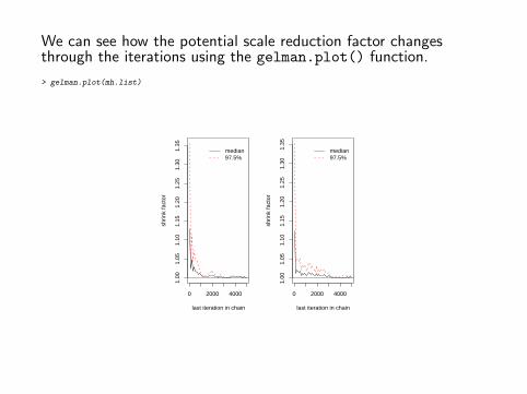
We can see how the potential scale reduction factor changesthrough the iterations using the gelman.plot() function.

> gelman.plot(mh.list)

0 2000 4000

1.00

1.05

1.10

1.15

1.20

1.25

1.30

1.35

last iteration in chain

shrin

k fa

ctor

median97.5%

0 2000 4000

1.00

1.05

1.10

1.15

1.20

1.25

1.30

1.35

last iteration in chain

shrin

k fa

ctor

median97.5%

Outline

Convergence

Visual Inspection


Geweke Diagnostic



Geweke Diagnostic

The Geweke diagnostic takes two nonoverlapping parts (usuallythe first 0.1 and last 0.5 proportions) of the Markov chain andcompares the means of both parts, using a difference of means testto see if the two parts of the chain are from the same distribution(null hypothesis).

The test statistic is a standard Z-score with the standard errorsadjusted for autocorrelation.

> geweke.diag(mh.draws)

Fraction in 1st window = 0.1

Fraction in 2nd window = 0.5

var1 var2

0.6149 0.1035

Outline

Convergence

Visual Inspection


Geweke Diagnostic




Suppose we want to measure some posterior quantile of interest q.

If we define some acceptable tolerance r for q and a probability sof being within that tolerance, the Raftery and Lewis diagnosticwill calculate the number of iterations N and the number ofburn-ins M necessary to satisfy the specified conditions.

The diagnostic was designed to test the number of iterations andburn-in needed by first running and testing shorter pilot chain.

In practice, we can also just test our normal chain to see if itsatisfies the results that the diagnostic suggests.

Inputs:

1. Select a posterior quantile of interest q (for example, the0.025 quantile).

2. Select an acceptable tolerance r for this quantile (for example,if r = 0.005, then that means we want to measure the 0.025quantile with an accuracy of ±0.005).

3. Select a probability s, which is the desired probability of beingwithin (q-r, q+r).

4. Run a“pilot” sampler to generate a Markov chain of minimumlength given by rounding up

nmin =

[Φ−1

(s + 1

2

) √q(1− q)

r

]2

where Φ−1(·) is the inverse of the normal CDF.

Results:

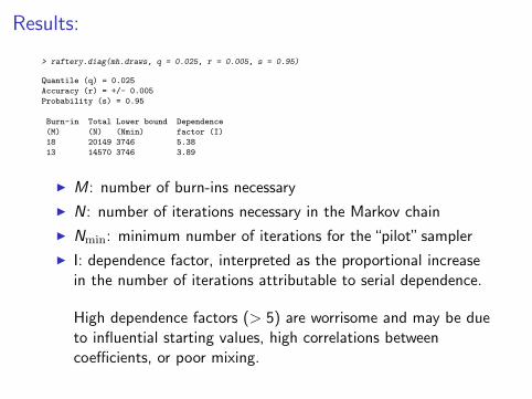
> raftery.diag(mh.draws, q = 0.025, r = 0.005, s = 0.95)

Quantile (q) = 0.025

Accuracy (r) = +/- 0.005

Probability (s) = 0.95

Burn-in Total Lower bound Dependence

(M) (N) (Nmin) factor (I)

18 20149 3746 5.38

13 14570 3746 3.89

I M: number of burn-ins necessary

I N: number of iterations necessary in the Markov chain

I Nmin: minimum number of iterations for the“pilot” sampler

I I: dependence factor, interpreted as the proportional increasein the number of iterations attributable to serial dependence.

High dependence factors (> 5) are worrisome and may be dueto influential starting values, high correlations betweencoefficients, or poor mixing.

The Raftery-Lewis diagnostic will differ depending on whichquantile q you choose.

Estimates tend to be conservative in that it will suggest moreiterations than necessary.

It only tests marginal convergence on each parameter.

Nevertheless, it often works well with simple models.

Outline

Convergence

Visual Inspection


Geweke Diagnostic




The Heidelberg and Welch diagnostic calculates a test statistic(based on the Cramer-von Mises test statistic) to accept or rejectthe null hypothesis that the Markov chain is from a stationarydistribution.

The diagnostic consists of two parts.

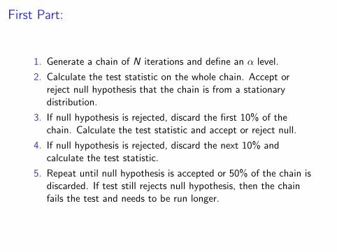
First Part:

1. Generate a chain of N iterations and define an α level.

2. Calculate the test statistic on the whole chain. Accept orreject null hypothesis that the chain is from a stationarydistribution.

3. If null hypothesis is rejected, discard the first 10% of thechain. Calculate the test statistic and accept or reject null.

4. If null hypothesis is rejected, discard the next 10% andcalculate the test statistic.

5. Repeat until null hypothesis is accepted or 50% of the chain isdiscarded. If test still rejects null hypothesis, then the chainfails the test and needs to be run longer.

Second Part:

If the chain passes the first part of the diagnostic, then it takes thepart of the chain not discarded from the first part to test thesecond part.

The halfwidth test calculates half the width of the (1− α)%credible interval around the mean.

If the ratio of the halfwidth and the mean is lower than some ε,then the chain passes the test. Otherwise, the chain must be runout longer.

> heidel.diag(mh.draws)

Stationarity start p-value

test iteration

var1 passed 1 0.834

var2 passed 1 0.693

Halfwidth Mean Halfwidth

test

var1 passed 3.03 0.0756

var2 passed 1.00 0.0805

Convergence Diagnostics - Patrick Lampatricklam.org/teaching/convergence_print.pdfAnother way to...

Documents

Transcript of Convergence Diagnostics - Patrick Lampatricklam.org/teaching/convergence_print.pdfAnother way to...