Convergence Analysis of Deterministic and … Analysis of Deterministic and Stochastic Methods for...
72
Convergence Analysis of Deterministic and Stochastic Methods for Convex Optimization by Riley Brooks A final project submitted to the Department of Applied Mathematics in partial fulfillment of the requirements for the degree of Master’s of Mathematics (MMath) Department of Applied Mathematics University of Waterloo August 2017 Waterloo Ontario
Transcript of Convergence Analysis of Deterministic and … Analysis of Deterministic and Stochastic Methods for...
Convergence Analysis of Deterministic
and Stochastic Methods for Convex
Optimization
by
Riley Brooks
A final project submitted to the
Department of Applied Mathematics
in partial fulfillment of the
requirements for the degree of
Master’s of Mathematics (MMath)
Department of Applied Mathematics
University of Waterloo
August 2017
Waterloo Ontario
Abstract
Numerous scientific problems can be formulated in terms of optimizing a convex objective func-
tion. As such, the study and developement of algorithms designed to solve these problems is of
considerable importance. This project attempts to act as an introduction to a selected number of
well known optimization algorithms by examining convergence results of deterministic and stochas-
tic algorithms. The concept of momentum is discussed and shown to have significant impact on
convergence. Throughout, it should become clear that deterministic methods which have been
known for decades are of fundamental importance for developing methods which noticably reduce
the computational complexity while preserving fast convergence. Several methods are shown to
achieve known optimal rates for a certain classes of algorithms. This is concluded with a variety of
numerical examples to illustrate the comparative performance of the algorithms presented.

Acknowledgments
I would like to extend my deepest thank you and appreciation to my supervisor Dr. Jun Liu
for his guidance and support during my time as a graduate student. I am grateful to have been
given the opportunity to advance my academic career. It has been a pleasure to work in such an
interdisciplinary environment, and what I have learned will be invaluable for my future career path.
A special thank you to Dr. Xinzhi Liu for contributing his time and expertise to reviewing this
paper.
Table of Contents
Abstract ii
Acknowledgments iii
List of Figures viii
1 Introduction 1
1.1 Motivation . . . . . . . . . . . . . . . . . . . . . . . . . . . . . . . . . . . . . . . . . 1
1.2 Outline . . . . . . . . . . . . . . . . . . . . . . . . . . . . . . . . . . . . . . . . . . . 3
2 Definitions and Inequalities 4
2.1 Lipschitz Continuity . . . . . . . . . . . . . . . . . . . . . . . . . . . . . . . . . . . 4
2.2 Convexity . . . . . . . . . . . . . . . . . . . . . . . . . . . . . . . . . . . . . . . . . 5
2.3 Expectation . . . . . . . . . . . . . . . . . . . . . . . . . . . . . . . . . . . . . . . . 7
3 Deterministic Methods 8
v
3.1 Gradient Descent . . . . . . . . . . . . . . . . . . . . . . . . . . . . . . . . . . . . . 8
3.1.1 General Convexity . . . . . . . . . . . . . . . . . . . . . . . . . . . . . . . . 9
3.1.2 Strong Convexity . . . . . . . . . . . . . . . . . . . . . . . . . . . . . . . . . 11
3.2 Nesterov Accelerated Gradient . . . . . . . . . . . . . . . . . . . . . . . . . . . . . . 12
3.2.1 General Convexity . . . . . . . . . . . . . . . . . . . . . . . . . . . . . . . . 14
3.2.2 Strong Convexity . . . . . . . . . . . . . . . . . . . . . . . . . . . . . . . . . 16
3.3 Newton’s Method . . . . . . . . . . . . . . . . . . . . . . . . . . . . . . . . . . . . . 21
3.3.1 General Convexity . . . . . . . . . . . . . . . . . . . . . . . . . . . . . . . . 22
4 Stochastic Optimization 25
4.1 Stochastic Gradient Descent . . . . . . . . . . . . . . . . . . . . . . . . . . . . . . . 26
4.1.1 General Convex . . . . . . . . . . . . . . . . . . . . . . . . . . . . . . . . . . 27
4.1.2 Strong Convexity . . . . . . . . . . . . . . . . . . . . . . . . . . . . . . . . . 28
4.2 Randomized Coordinate Gradient Descent . . . . . . . . . . . . . . . . . . . . . . . 31
4.2.1 General Convexity . . . . . . . . . . . . . . . . . . . . . . . . . . . . . . . . 32
4.2.2 Strong Convexity . . . . . . . . . . . . . . . . . . . . . . . . . . . . . . . . . 34
4.3 Accelerated Randomized Coordinate Gradient Descent . . . . . . . . . . . . . . . . 35
4.4 ADAM . . . . . . . . . . . . . . . . . . . . . . . . . . . . . . . . . . . . . . . . . . . 39
4.5 AdaGrad . . . . . . . . . . . . . . . . . . . . . . . . . . . . . . . . . . . . . . . . . . 46
5 Numerical Examples 48

vi
5.1 Ball Shaped . . . . . . . . . . . . . . . . . . . . . . . . . . . . . . . . . . . . . . . . 49
5.1.1 Sum of Squares Function . . . . . . . . . . . . . . . . . . . . . . . . . . . . . 49
5.1.2 Bohachevsky-1 function . . . . . . . . . . . . . . . . . . . . . . . . . . . . . 50
5.2 Plate Shaped . . . . . . . . . . . . . . . . . . . . . . . . . . . . . . . . . . . . . . . 52
5.2.1 Booth Function . . . . . . . . . . . . . . . . . . . . . . . . . . . . . . . . . . 52
5.2.2 McCormick Function . . . . . . . . . . . . . . . . . . . . . . . . . . . . . . . 53
5.3 Functions with Many Local Minima . . . . . . . . . . . . . . . . . . . . . . . . . . . 55
5.3.1 Ackley Function . . . . . . . . . . . . . . . . . . . . . . . . . . . . . . . . . . 55
5.3.2 Levy Function . . . . . . . . . . . . . . . . . . . . . . . . . . . . . . . . . . . 57
5.4 Additional Functions . . . . . . . . . . . . . . . . . . . . . . . . . . . . . . . . . . . 59
5.4.1 Beale Function . . . . . . . . . . . . . . . . . . . . . . . . . . . . . . . . . . 59
5.4.2 Styblinski-Tang 2D . . . . . . . . . . . . . . . . . . . . . . . . . . . . . . . . 60
List of Figures
5.1 Plots of the Sum of Squares function on the domain x, y ∈ [−5, 5] along with conver-
gence plot of all algorithms discussed. . . . . . . . . . . . . . . . . . . . . . . . . . . 50
5.2 Plots of the Bohachevsky function on the domain x, y ∈ [−100, 100] along with
convergence plot of all algorithms discussed. . . . . . . . . . . . . . . . . . . . . . . 51
5.3 Plots of the Booth function on the domain x, y ∈ [−5, 5] along with convergence plot
of all algorithms discussed. . . . . . . . . . . . . . . . . . . . . . . . . . . . . . . . . 53
5.4 Plots of the McCormick function on the domain x, y ∈ [−5, 5] along with convergence
plot of all algorithms discussed. . . . . . . . . . . . . . . . . . . . . . . . . . . . . . 55
5.5 Plots of the Ackley function on the domain x, y ∈ [−5, 5] along with convergence plot
of all algorithms discussed. . . . . . . . . . . . . . . . . . . . . . . . . . . . . . . . . 57
5.6 Plots of the Levy function on the domain x, y ∈ [−5, 5] along with convergence plot
of all algorithms discussed. . . . . . . . . . . . . . . . . . . . . . . . . . . . . . . . . 58
5.7 Plots of the Beale function on the domain x, y ∈ [−5, 5] along with convergence plot
of all algorithms discussed. . . . . . . . . . . . . . . . . . . . . . . . . . . . . . . . . 60
viii
5.8 . . . . . . . . . . . . . . . . . . . . . . . . . . . . . . . . . . . . . . . . . . . . . . . 61
5.9 Plots of convergence results for deterministic and stochastic methods on the Styblinski-
Tang function over the domain x, y ∈ [−5, 5]. . . . . . . . . . . . . . . . . . . . . . . 62
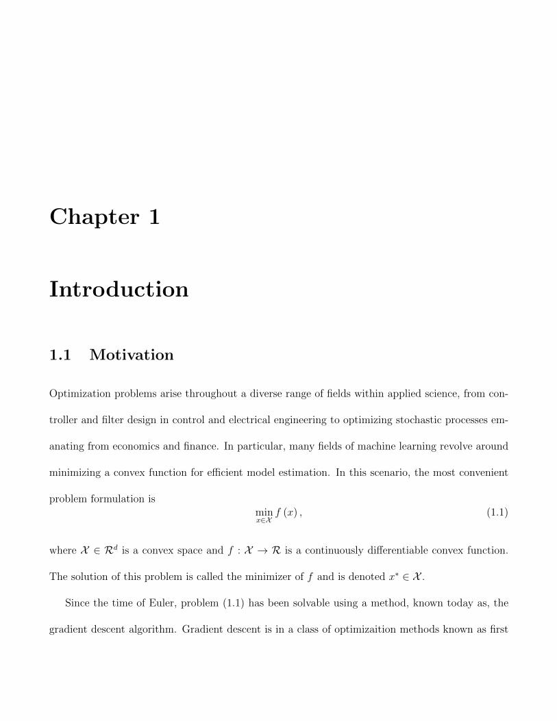
Chapter 1
Introduction
1.1 Motivation
Optimization problems arise throughout a diverse range of fields within applied science, from con-
troller and filter design in control and electrical engineering to optimizing stochastic processes em-
anating from economics and finance. In particular, many fields of machine learning revolve around
minimizing a convex function for efficient model estimation. In this scenario, the most convenient
problem formulation isminx∈X
f (x) , (1.1)
where X ∈ Rd is a convex space and f : X → R is a continuously differentiable convex function.
The solution of this problem is called the minimizer of f and is denoted x∗ ∈ X .
Since the time of Euler, problem (1.1) has been solvable using a method, known today as, the
gradient descent algorithm. Gradient descent is in a class of optimizaition methods known as first
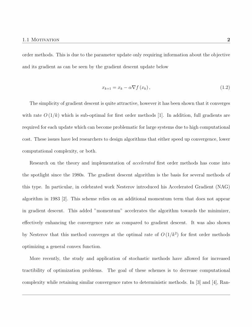
1.1 Motivation 2
order methods. This is due to the parameter update only requiring information about the objective
and its gradient as can be seen by the gradient descent update below
xk+1 = xk − α∇f (xk) , (1.2)
The simplicity of gradient descent is quite attractive, however it has been shown that it converges
with rate O (1/k) which is sub-optimal for first order methods [1]. In addition, full gradients are
required for each update which can become problematic for large systems due to high computational
cost. These issues have led researchers to design algorithms that either speed up convergence, lower
computational complexity, or both.
Research on the theory and implementation of accelerated first order methods has come into
the spotlight since the 1980s. The gradient descent algorithm is the basis for several methods of
this type. In particular, in celebrated work Nesterov introduced his Accelerated Gradient (NAG)
algorithm in 1983 [2]. This scheme relies on an additional momentum term that does not appear
in gradient descent. This added ”momentum” accelerates the algorithm towards the minimizer,
effectively enhancing the convergence rate as compared to gradient descent. It was also shown
by Nesterov that this method converges at the optimal rate of O (1/k2) for first order methods
optimizing a general convex function.
More recently, the study and application of stochastic methods have allowed for increased
tractibility of optimization problems. The goal of these schemes is to decrease computational
complexity while retaining similar convergence rates to deterministic methods. In [3] and [4], Ran-
1.2 Outline 3
domized Coordinate Gradient Descent (RCGD) was introduced to handle high dimensional problems
with a lower computational complexity than gradient descent. Shortly after, an accelerated version
of RCGD, called Accelerate Randomized Coordinate Gradient (ARCG) was proposed in [5]. The
proposal of these algorithms displayed how well known deterministic methods can be used to design
stochastic ones.
The most recent developements in optimization stretch this idea to use statistical moment
estimation to solve huge, sparse problems. Two such methods of this type are Adam and Adagrad
which were first introduced in [6] and [7] respectively. They use estimations of the mean and
uncentered variance of the gradient in place of the using the full gradient. As with RCGD and
ARCD, the goal is to lower the computational complexity while also holding on to quick convergence.
1.2 Outline
This project will proceed as follows, Chapter 2 will cover basic definitions, such as Lipschitz con-
tinuity and convexity, that will be required for all subsequent chapters. Chapter 3 will cover the
algorithms and convergence analysis of the most well known deterministic methods. In particular,
convergence results for Gradient Descent, Nesterov Accelerated Gradient and Newton’s Method
will be established for weakly and strongly convex objective function. Chapter 4 covers several
stochastic algorithms and proceeds in the same manner as chapter 3. Finally, numerical tests for all
methods covered will be presented and analyzed. The goal is to present a unified survey of several
deterministic and stochastic optimization algorithms commonly used or discussed in the literature.
Chapter 2
Definitions and Inequalities
2.1 Lipschitz Continuity
This property is extremely useful for convergence analysis as it provides access to several convenient
inequalities, especially when paired with convexity. It will be assumed throughout that f(x), and in
the case of stochastic optimization, each sub-function fi (x) will have Lipschitz continuous gradient.
Definition 2.0.1. A function f : Rd → R is Lipschitz Continuous with Lipschitz factor L if and
only if the following inequalities hold for all x, y ∈ Rd,
‖f (x)− f (y) ‖ ≤ L‖x− y‖, (2.1)
f (y) ≤ f (x) + 〈∇f (x) , y − x〉+L
2‖y − x‖2, (2.2)
2.2 Convexity 5
The two inequalities above are equivalent, so either can be used to represent Lipschitz continuity.
If, in addition, f (x) is twice differentiable then it is also true that ∇2f (x) ≤ LId, where Id is the
d× d identity matrix.
2.2 Convexity
If a function is known to be convex then it satisfies several inequalities that are practical when deriv-
ing convergence rates for optimization algorithms. Since this project’s focus is convex optimization
these inequalities are listed below for convenience. As mentioned previously, the combination of
convexity and Lipschitz continuity implies a function satisfies a wide selection of inequalities. The
definition for convexity and subsequent inequalities now follows.
Definition 2.0.2. Let χ ⊆ Rd be a convex set, a function f : χ → R is convex if ∀x, y ∈ χ,
∀α ∈ [0, 1]f (αx+ (1− α) y) ≤ αf (x) + (1− α) f (y) . (2.3)
This definition simply implies that a line segment connecting any two points of a function lies
above or on the graph of the function. This is especially important for convex optimization since
if f is differentiable then all stationary points of f are global minima. In this case, two additional
inequalities arise which are equivalent to f being convex.
f (y) ≥ f (x) +∇f (x) · (y − x) (2.4)
(∇f (x)−∇f (y)) · (x− y) ≥ 0 (2.5)
2.2 Convexity 6
In the case where f is twice differentiable, ∇2f (x) � 0, is equivalent to the definition above. Com-
bining the definitions of convexity and Lipschitz continuity of the gradient yields several practical
inequalities which will be used in later chapters and are listed below. As in the individual definitions
for convexity and Lipschitz continuity, if f is twice differentiable then all of the above are equivalent
to 0 � ∇2f (x) � LId.
0 ≤ f (y)− f (x)− 〈∇f (x) , y − x〉 ≤ L
2‖y − x‖2 (2.6)
f (y) ≥ f (x) + 〈∇f (x) , y − x〉+1
2L‖∇f (y)−∇f (x) ‖2 (2.7)
0 ≤ 〈∇f (x)−∇f (y) , x− y〉 ≤ L‖y − x‖2 (2.8)
〈∇f (y)−∇f (x) , y − x〉 ≥ 1
L‖∇f (y)−∇f (x) ‖2 (2.9)
Definition 2.0.3. A function f : Rd → R is strongly convex with convexity parameter µ if and
only if the following hold.
f (y)− f (x)−∇f (x) · (y − x)− µ
2‖y − x‖2 ≥ 0 (2.10)
(∇f (y)−∇f (x)) · (y − x)− µ‖y − x‖2 ≥ 0 ∀x, y ∈ R (2.11)
Once again, if f is twice differentiable there is another inequality, namely ∇2f (x) � µId.
2.3 Expectation 7
2.3 Expectation
Also known as expected value, the expectation of a discrete random variable is the probability
weighted average of all possible values. In the section on stochastic optimization the discrete random
variable will be denoted ik where i corresponds to an element of the gradient vector (a particular
dimension where i ∈ 1, . . . , d). The subscript k represents the iteration count, as such ik represents
the set of randomly selected coordinates during the kth iteration of the algorithm. Alternatively,
one could find the expectation with respect to ik over all k ∈ 1, . . . , K which is denoted as ξk−1 for
convenience. A short-hand that is used for this form of the expectation is φk = Eξk−1[f (xk)].
In all cases, the expectation with respect to the kth iteration (i.e. expectation w.r.t ik) is
considered first. It then follows that to complete the convergence inequality one must take the
expectation over all iterations, hence the need for the notation ξk−1. It is important to note that the
probability of selecting a particular coordinate is uniformly distributed so the probability weighted
average will be
Eik [f (xk)] =n∑i=1
p(i) · fi (xk) , p(i) =1
n.
Chapter 3
Deterministic Methods
3.1 Gradient Descent
In all likelihood, Gradient Descent was the first known method for finding optimal values of a
function. Whether or not this is the case, gradient descent is the foundation for most determinsitic
optimization methods as well as many well known stochastic schemes. As such, it is appropriate
to begin any general discussion of optimization algorithms with the gradient descent method. The
method is described by the iterative scheme below where αk is the time step and is optimally chosen
as α = 1L
:xk+1 = xk − αk∇f (xk) , (3.1)
Every algorithm discussed in this project, except Adam and Adagrad, will in some way include
this type of iterative step. Expectedly, the analysis for GD is much simpler than all susbequent
3.1 Gradient Descent 9
algorithms but will still provide useful intuition for when it comes time to analyze the remaining
methods. Since the main purpose of this report is to review methods for convex optimization we
begin with considering the case where the objective f is a general convex function.
3.1.1 General Convexity
A simple manipulation of the definition for Lipschitz continuity, given by (2.2), through the gradient
descent update rule yields another helpful inequality for this section.
f (xk+1)− f (xk) ≤ −1
L(∇f (xk) ,∇f (xk)) +
1
2L||∇f (xk)||2
= − 1
2L||∇f (xk)||2 (3.2)
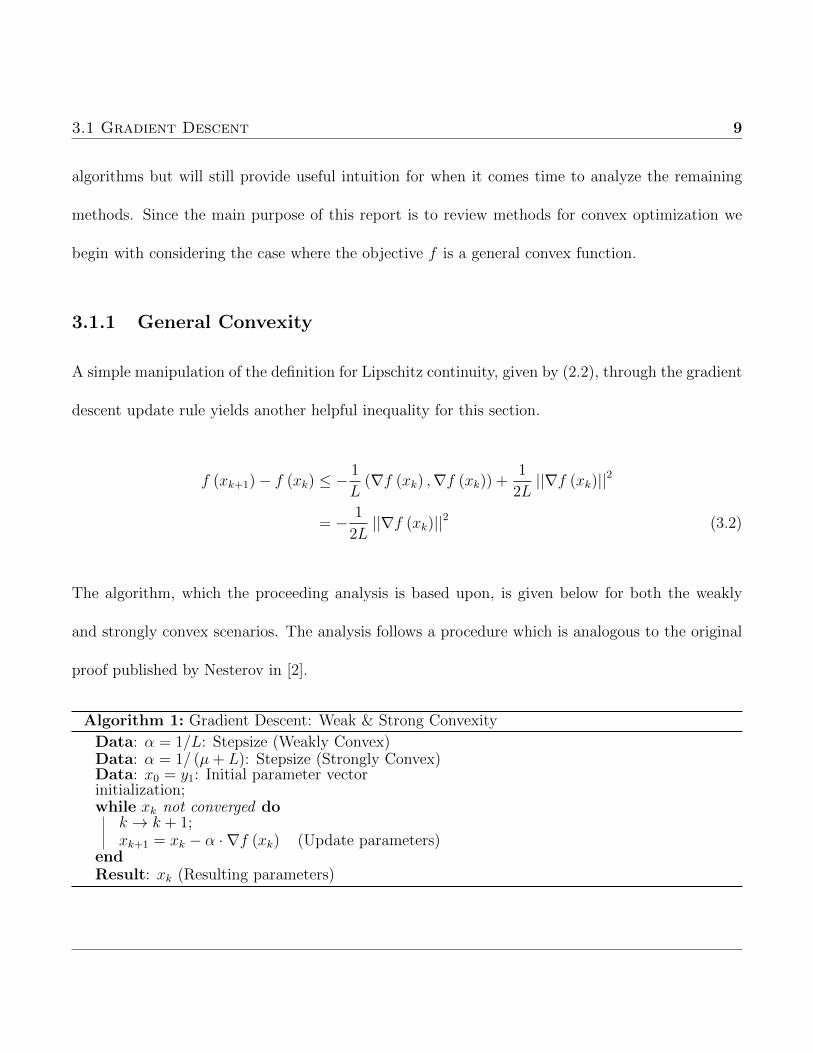
The algorithm, which the proceeding analysis is based upon, is given below for both the weakly
and strongly convex scenarios. The analysis follows a procedure which is analogous to the original
proof published by Nesterov in [2].
Algorithm 1: Gradient Descent: Weak & Strong Convexity
Data: α = 1/L: Stepsize (Weakly Convex)Data: α = 1/ (µ+ L): Stepsize (Strongly Convex)Data: x0 = y1: Initial parameter vectorinitialization;while xk not converged do
k → k + 1;xk+1 = xk − α · ∇f (xk) (Update parameters)
endResult: xk (Resulting parameters)
3.1 Gradient Descent 10
Theorem 3.1. Assume f is convex and has L-Lipschitz continuous gradient. Then the gradient
descent method with step size α = 1L
has the following global convergence rate
f (xk)− f ∗ ≤L
2k‖x0 − x∗‖2. (3.3)
Proof. We begin by subtracting f ∗ from both sides of (3.2) and take advantage of the convexity of
f .
f (xk+1)− f ∗ ≤ f (xk)− f ∗ −1
2L‖∇f (xk) ‖2
≤ 〈∇f (xk) , xk − x∗〉 −1
2L‖∇f (xk) ‖2
Now, use the GD update rule with a time step of 1L
and rearrange the resulting inequality.
f (xk+1)− f ∗ ≤ −L〈xk − x∗, xk+1 − xk〉 −L
2‖xk+1 − x∗‖2
= −L2
[xk+1 − x∗ + xk − x∗] · [xk+1 − x∗ − xk + x∗]
=L
2
[‖xk − x∗‖2 − ‖xk+1 − x∗‖2
]
Sum the inequality resulting from the last line from 0 to k − 1.
k−1∑k=0
(f (xk+1)− f ∗) ≤L
2
[‖x0 − x∗‖2 − ‖xk − x∗‖2
]f (xk)− f ∗ ≤
L
2k‖x0 − x∗‖2
3.1 Gradient Descent 11
Thus the expected sublinear convergence rate given by (3.3) is obtained.
3.1.2 Strong Convexity
The method shown here is primarily taken from Nesterov’s book on convex optimization [1]. To
begin, it is convenient to derive an inequality to use as a starting point for the proof.
‖xk+1 − x∗‖2 = ‖xk − x∗ − α∇f (xk) ‖2
= ‖xk − x∗‖2 − 2α〈∇f (xk) , xk − x∗〉+ α2‖∇f (xk) ‖2
≤ ‖xk − x∗‖2 −2αµL
µ+ L‖xk − x∗‖2 +
(α2 − 2α
µ+ L
)‖∇f (xk) ‖2 (3.4)
where the last inequality is due to
〈∇f (xk) , xk − x∗〉 ≥µL
µ+ L‖xk − x∗‖2 +
1
µ+ L‖∇f (xk) ‖2
Theorem 3.2. Assume f is convex with strong convexity parameter µ. Additionally, f has L-
Lipschitz continuous gradient and consider using a step size α = 2µ+L
. Then GD convereges linearly
as
‖xk+1 − x∗‖2 ≤(µ− Lµ+ L
)2
‖xk − x∗‖2. (3.5)
Proof. Setting the step size in (3.4) as α = 2µ+L
leads to
3.2 Nesterov Accelerated Gradient 12
‖xk+1 − x∗‖2 ≤(
1− 4µL
(µ+ L)2
)‖xk − x∗‖2
≤(µ− Lµ+ L
)2
‖xk − x∗‖2.
This implies GD converges linearly with rate µ−Lµ+L
.
3.2 Nesterov Accelerated Gradient
In recent years, momentum methods have come to play a powerful role in optimization. Intuitively,
momentum arises by adding a weighted version of the previously iterated step of an algorithm
to the current one. Applied to the gradient descent scheme, whose continuous time counterpart
is represented by the gradient flow dynamics x = ∇f (x), momentum leads to a second-order
DE when transitioning to continuous time. In a sense, one can interpret this physically as a
massive particle moving in a potential well as noted in [8]. This system exhibits acceleration due
to the presence of a second derivative term. As such momentum methods are said to accelerate
an algorithm towards the minimizer and are therefore expected to obtain faster convergence than
methods without momentum. In fact, for first order methods the optimal convergence rate is
O (1/k2) which is indeed quicker than gradient descent which achieves O (1/k) convergence. With
the publishing of Nesterov’s 1983 paper [2], NAG became the only known algorithm to achieve
the optimal convergence rate for first order optimization methods. This algorithm relies strongly
on gradient descent but rather than simply taking the most recently iterated solution, NAG uses
a convex combination of the current and previous solution vectors. In essence, this added step
3.2 Nesterov Accelerated Gradient 13
provides the algorithm momentum which accelerates the process towards finding the minimizer.
The iterative scheme involved in this process is given below:
xk+1 = yk − αk∇f (yk)
yk+1 = xk+1 + βk (xk+1 − xk) (3.6)
The value for βk depends on whether the objective is weakly or strongly convex. In [9], βk = k−1k+2
for f weakly convex and in [1], βk =√L−√µ√L+√µ
for strongly convex. In both cases αk ≤ 1L
where the
optimal choice is αk = 1L
.
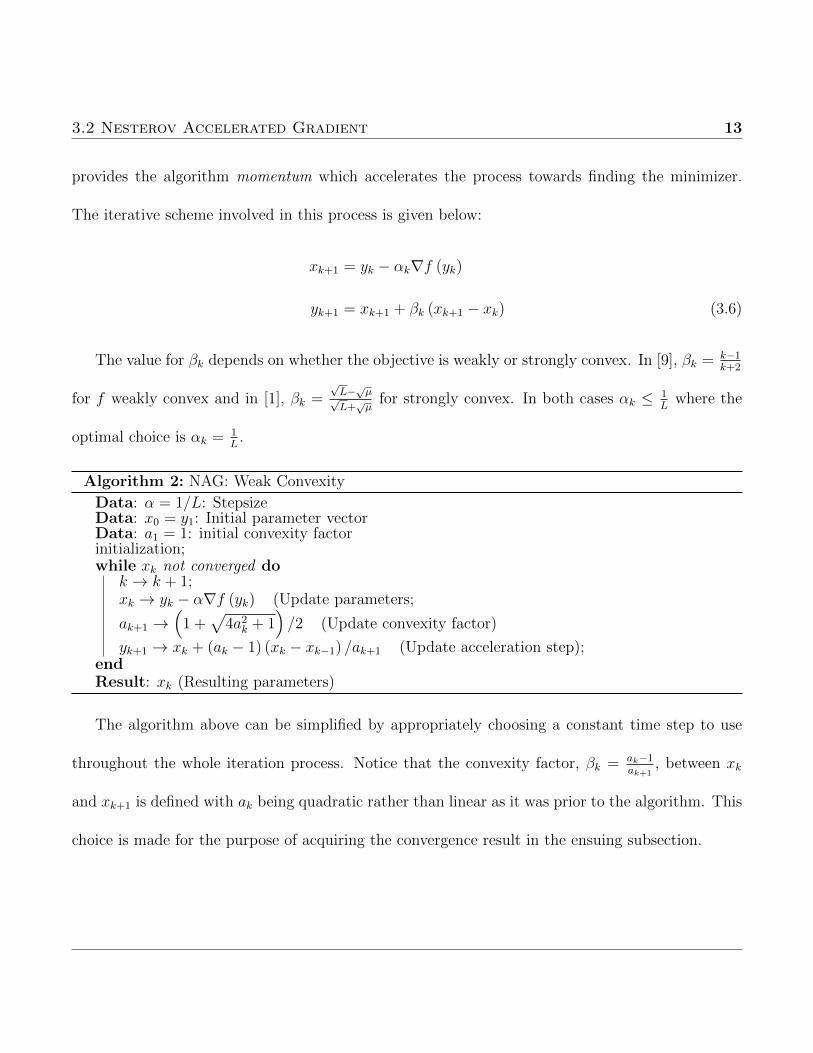
Algorithm 2: NAG: Weak Convexity
Data: α = 1/L: StepsizeData: x0 = y1: Initial parameter vectorData: a1 = 1: initial convexity factorinitialization;while xk not converged do
k → k + 1;xk → yk − α∇f (yk) (Update parameters;
ak+1 →(
1 +√
4a2k + 1)/2 (Update convexity factor)
yk+1 → xk + (ak − 1) (xk − xk−1) /ak+1 (Update acceleration step);endResult: xk (Resulting parameters)
The algorithm above can be simplified by appropriately choosing a constant time step to use
throughout the whole iteration process. Notice that the convexity factor, βk = ak−1ak+1
, between xk
and xk+1 is defined with ak being quadratic rather than linear as it was prior to the algorithm. This
choice is made for the purpose of acquiring the convergence result in the ensuing subsection.
3.2 Nesterov Accelerated Gradient 14
3.2.1 General Convexity
Theorem 3.3. Assume f : Rd → R is convex, has L-Lipschitz continuous gradient and has a
non-empty solution set. Then Nesterov’s accelerated gradient descent algorithm satisfies
f (xk)− f ∗ ≤4L‖y0 − x∗‖2
(k + 2)2(3.7)
Proof. We begin by mentioning an inequality that can be obtained in the same manner as (3.2)
while not choosing a constant time step.
f (yk)− f (xk) ≥1
2αk (2− αkL) ‖∇f (y − k) ‖2 (3.8)
Next, let zk = (ak − 1) (xk−1 − xk). Then yk+1 = xk− 1ak+1
zk, which implies zk+1−xk+1 = zk−xk +
ak+1αk+1∇f (yk + 1). Given this, the following holds
‖zk+1 − xk+1 + x∗‖2 = ‖zk − xk + x∗ + x∗ + ak+1αk+1∇f (yk+1) ‖2
= ‖zk − xk + x∗‖2 + 2ak+1αk+1〈∇f (yk+1) , zk − xk + x∗〉|a2k+1α2k+1‖∇f (yk+1) ‖2
= ‖zk − xk + x∗‖2 + 2ak+1αk+1〈∇f (yk+1) , zk〉
+ 2ak+1αk+1〈∇f (yk+1) , x∗ − xk〉+ a2k+1α
2k+1‖∇f (yk+1) ‖2
= ‖zk − xk + x∗‖2 + 2 (ak+1 − 1)αk+1〈∇f (yk+1) , zk〉
+ 2ak+1αk+1〈∇f (yk+1) , x∗ − yk+1〉+ a2k+1α
2k+1‖∇f (yk+1) ‖2.
(3.9)
3.2 Nesterov Accelerated Gradient 15
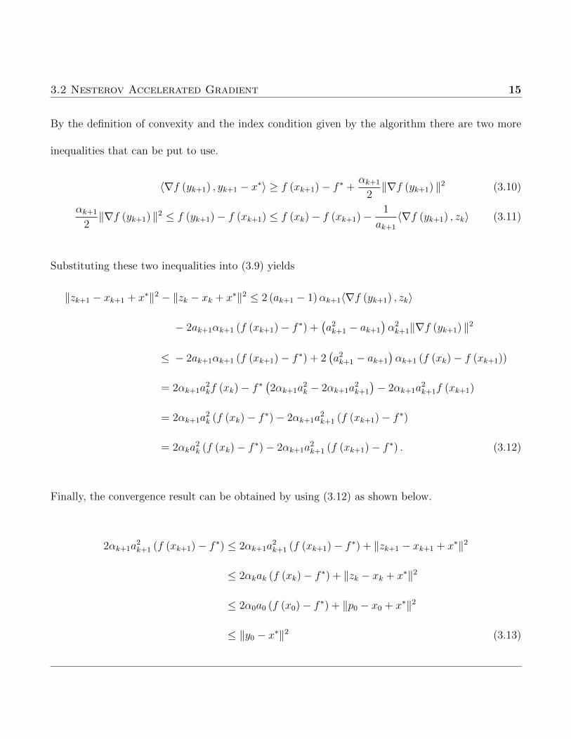
By the definition of convexity and the index condition given by the algorithm there are two more
inequalities that can be put to use.
〈∇f (yk+1) , yk+1 − x∗〉 ≥ f (xk+1)− f ∗ +αk+1
2‖∇f (yk+1) ‖2 (3.10)
αk+1
2‖∇f (yk+1) ‖2 ≤ f (yk+1)− f (xk+1) ≤ f (xk)− f (xk+1)−
1
ak+1
〈∇f (yk+1) , zk〉 (3.11)
Substituting these two inequalities into (3.9) yields
‖zk+1 − xk+1 + x∗‖2 − ‖zk − xk + x∗‖2 ≤ 2 (ak+1 − 1)αk+1〈∇f (yk+1) , zk〉
− 2ak+1αk+1 (f (xk+1)− f ∗) +(a2k+1 − ak+1
)α2k+1‖∇f (yk+1) ‖2
≤ − 2ak+1αk+1 (f (xk+1)− f ∗) + 2(a2k+1 − ak+1
)αk+1 (f (xk)− f (xk+1))
= 2αk+1a2kf (xk)− f ∗
(2αk+1a
2k − 2αk+1a
2k+1
)− 2αk+1a
2k+1f (xk+1)
= 2αk+1a2k (f (xk)− f ∗)− 2αk+1a
2k+1 (f (xk+1)− f ∗)
= 2αka2k (f (xk)− f ∗)− 2αk+1a
2k+1 (f (xk+1)− f ∗) . (3.12)
Finally, the convergence result can be obtained by using (3.12) as shown below.
2αk+1a2k+1 (f (xk+1)− f ∗) ≤ 2αk+1a
2k+1 (f (xk+1)− f ∗) + ‖zk+1 − xk+1 + x∗‖2
≤ 2αkak (f (xk)− f ∗) + ‖zk − xk + x∗‖2
≤ 2α0a0 (f (x0)− f ∗) + ‖p0 − x0 + x∗‖2
≤ ‖y0 − x∗‖2 (3.13)
3.2 Nesterov Accelerated Gradient 16
(3.7) is obtained by noting that the index condition given by the algorithm is satisfied when αk ≤ 1L
,
so the time step will not decrease after this point. Thus, one can assume αk ≥ 12L
. Also notice,
from the definition for ak+1 one has ak+1 ≤ ak ≤ 0.5 ≤ a0 +∑k
k=1 0.5 = 1 + 0.5 (k + 1).
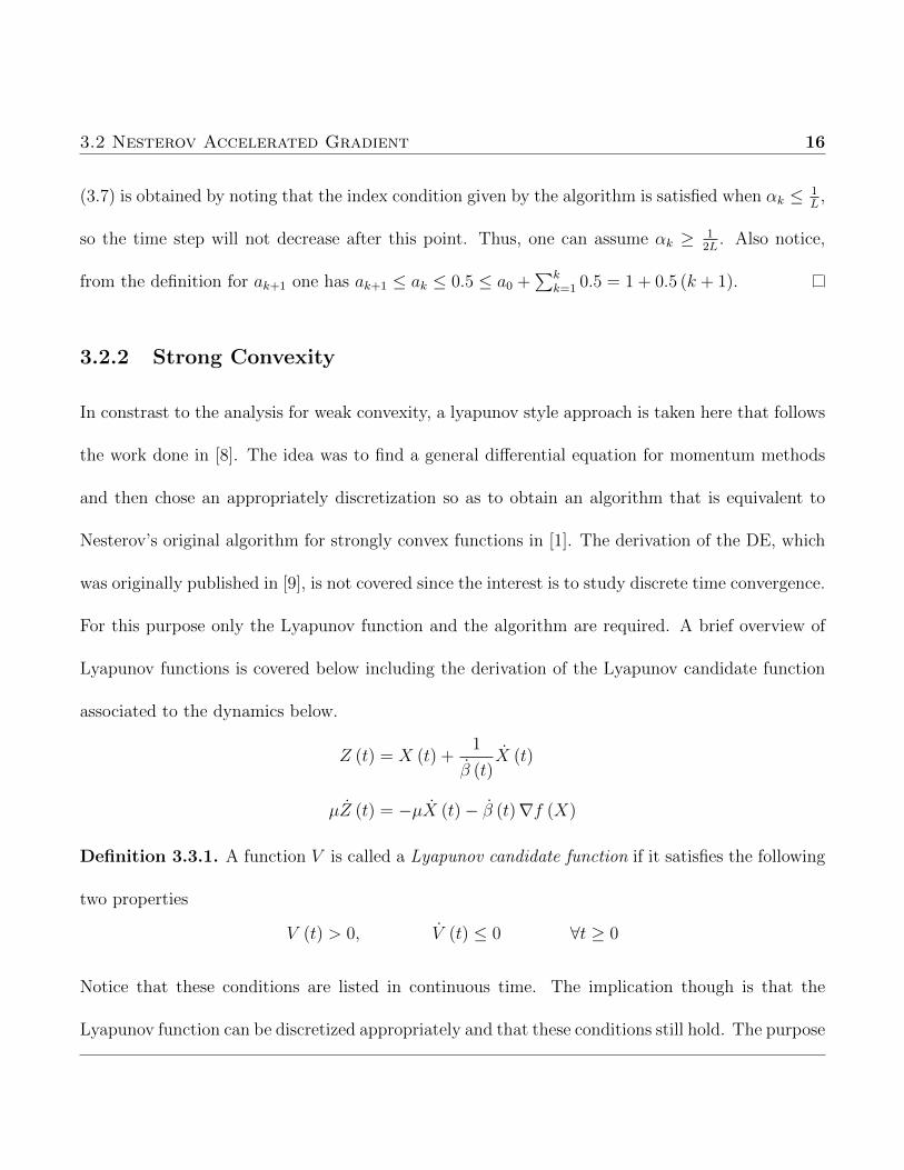
3.2.2 Strong Convexity
In constrast to the analysis for weak convexity, a lyapunov style approach is taken here that follows
the work done in [8]. The idea was to find a general differential equation for momentum methods
and then chose an appropriately discretization so as to obtain an algorithm that is equivalent to
Nesterov’s original algorithm for strongly convex functions in [1]. The derivation of the DE, which
was originally published in [9], is not covered since the interest is to study discrete time convergence.
For this purpose only the Lyapunov function and the algorithm are required. A brief overview of
Lyapunov functions is covered below including the derivation of the Lyapunov candidate function
associated to the dynamics below.
Z (t) = X (t) +1
β (t)X (t)
µZ (t) = −µX (t)− β (t)∇f (X)
Definition 3.3.1. A function V is called a Lyapunov candidate function if it satisfies the following
two properties
V (t) > 0, V (t) ≤ 0 ∀t ≥ 0
Notice that these conditions are listed in continuous time. The implication though is that the
Lyapunov function can be discretized appropriately and that these conditions still hold. The purpose
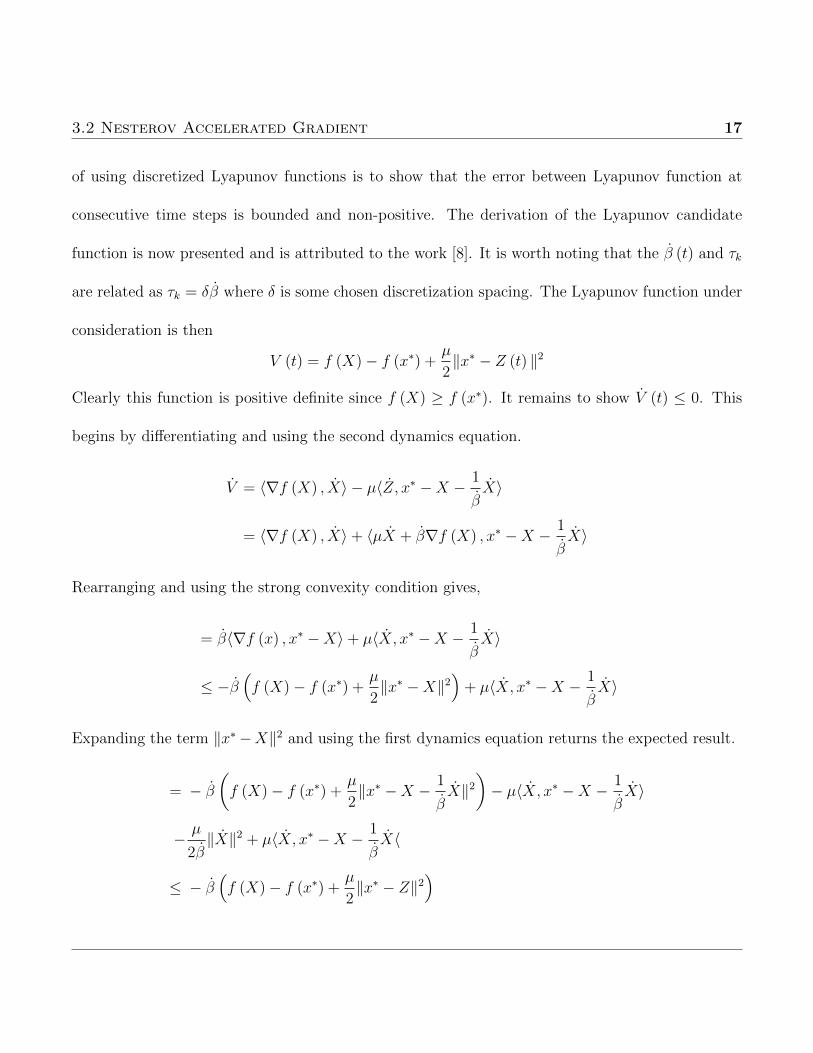
3.2 Nesterov Accelerated Gradient 17
of using discretized Lyapunov functions is to show that the error between Lyapunov function at
consecutive time steps is bounded and non-positive. The derivation of the Lyapunov candidate
function is now presented and is attributed to the work [8]. It is worth noting that the β (t) and τk
are related as τk = δβ where δ is some chosen discretization spacing. The Lyapunov function under
consideration is then
V (t) = f (X)− f (x∗) +µ
2‖x∗ − Z (t) ‖2
Clearly this function is positive definite since f (X) ≥ f (x∗). It remains to show V (t) ≤ 0. This
begins by differentiating and using the second dynamics equation.
V = 〈∇f (X) , X〉 − µ〈Z, x∗ −X − 1
βX〉
= 〈∇f (X) , X〉+ 〈µX + β∇f (X) , x∗ −X − 1
βX〉
Rearranging and using the strong convexity condition gives,
= β〈∇f (x) , x∗ −X〉+ µ〈X, x∗ −X − 1
βX〉
≤ −β(f (X)− f (x∗) +
µ
2‖x∗ −X‖2
)+ µ〈X, x∗ −X − 1
βX〉
Expanding the term ‖x∗−X‖2 and using the first dynamics equation returns the expected result.
= − β(f (X)− f (x∗) +
µ
2‖x∗ −X − 1
βX‖2
)− µ〈X, x∗ −X − 1
βX〉
− µ
2β‖X‖2 + µ〈X, x∗ −X − 1
βX〈
≤ − β(f (X)− f (x∗) +
µ
2‖x∗ − Z‖2
)
3.2 Nesterov Accelerated Gradient 18
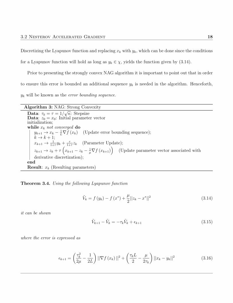
Discretizing the Lyapunov function and replacing xk with yk, which can be done since the conditions
for a Lyapunov function will hold as long as yk ∈ χ, yields the function given by (3.14).
Prior to presenting the strongly convex NAG algorithm it is important to point out that in order
to ensure this error is bounded an additional sequence yk is needed in the algorithm. Henceforth,
yk will be known as the error bounding sequence.
Algorithm 3: NAG: Strong Convexity
Data: τk = τ = 1/√κ: Stepsize
Data: z0 = x0: Initial parameter vectorinitialization;while xk not converged do
yk+1 → xk − 1L∇f (xk) (Update error bounding sequence);
k → k + 1;xk+1 → 1
1+τyk + τ
1+τzk (Parameter Update);
zk+1 → zk + τ(xk+1 − zk − 1
µ∇f (xk+1)
)(Update parameter vector associated with
derivative discretization);endResult: xk (Resulting parameters)
Theorem 3.4. Using the following Lyapunov function
Vk = f (yk)− f (x∗) +µ
2||zk − x∗||2 (3.14)
it can be shown
Vk+1 − Vk = −τkVk + εk+1 (3.15)
where the error is expressed as
εk+1 =
(τ 2k2µ− 1
2L
)||∇f (xk) ||2 +
(τkL
2− µ
2τk
)||xk − yk||2 (3.16)
3.2 Nesterov Accelerated Gradient 19
Proof. The error is required to be non-positive in order for Vk to satisfy the conditions of the Lya-
punov function. This results in the time step to be τk ≤ 1√κ, where equality yields the convergence
rate originally obtained by Nesterov for strongly convex functions.
Vk+1 − Vk = f (yk+1)− f (yk)− µ〈zk+1 − zk, x∗ − zk+1〉 −µ
2||zk+1 − zk||2
= f (yk+1)− f (xk) + f (xk)− f (yk)− µ〈zk+1 − zk, x∗ − zk〉+µ
2||zk+1 − zk||2
≤ f (yk+1)− f (xk) + 〈∇f (xk) , xk − yk〉 −µ
2||xk − yk||2 − µ〈zk+1 − zk, x∗ − zk〉+
µ
2||zk+1 − zk||2
= f (yk+1)− f (xk) + 〈∇f (xk) , xk − yk〉 −µ
2||xk − yk||2 +
1√κ〈∇f (xk)− µ (xk − zk) , x∗ − zk〉
+µ
2||zk+1 − zk||2
= f (yk+1)− f (xk) +1√κ〈∇f (xk) , x
∗ − xk〉 −µ
2||xk − yk||2 −
1√κµ〈xk − zk, x∗ − zk〉
+µ
2||zk+1 − zk||2
≤ − 1√κ
(f (xk)− f (x∗) +
µ
2||x∗ − xk||2
)+ f (yk+1)− f (xk)−
µ
2||xk − yk||2
− 1√κµ〈xk − zk, x∗ − zk〉+
µ
2||zk+1 − zk||2
Both inequalities above come from using the strong convexity property of f . The first equality
arises from the final line of Algorithm 3 while the last equality is due to the update for the error
bounding sequence.
In the succeeding analysis the first line is due to a simple manipulation of norms while the
subsequent two equalities come about due to the final line of Algorithm 3 and the parameter
update rule respectively. Both inequalities are a result of (2.6) which is based on the convexity and
3.2 Nesterov Accelerated Gradient 20
Lipschitz continuity of the objective.
Vk+1 − Vk = − 1√κ
(f (xk)− f (x∗) +
µ
2||x∗ − zk||2
)+ f (yk+1)− f (xk)−
µ
2||xk − yk||2 +
µ
2||zk+1 − zk||2
− µ
2√κ||xk − zk||2
= − 1√κ
(f (xk)− f (x∗) +
µ
2||x∗ − zk||2
)+ f (yk+1)− f (xk)−
µ
2||xk − yk||2
+µ
2|| 1√
κ(xk − zk) ||2 −
1√κ〈∇f (xk) ,
1√κ
(xk − zk)〉+1
2µκ||∇f (xk) ||2 −
µ√κ
2||xk − yk||2
= − 1√κ
(f (xk)− f (x∗) +
µ
2||x∗ − zk||2
)+ f (yk+1)− f (xk)−
1√κ〈∇f (xk) , yk − xk〉
+1
2µκ||∇f (xk) ||2 −
µ√κ
2||xk − yk||2
≤ − 1√κ
(f (xk)− f (x∗) +
µ
2||x∗ − zk||2
)+ f (yk+1)− f (xk)−
1√κ
(f (yk)− f (xk))
+1
2µκ||∇f (xk) ||2 +
(L
2√κ− µ√κ
2
)||xk − yk||2
= − 1√κ
(f (yk)− f (x∗) +
µ
2||x∗ − zk||2
)+ f (yk+1)− f (xk) +
1
2µκ||∇f (xk) ||2
+
(L
2√κ− µ√κ
2
)||xk − yk||2
≤ − 1√κ
(f (yk)− f (x∗) +
µ
2||x∗ − zk||2
)+
(1
2µκ− 1
2L
)||∇f (xk) ||2
+
(L
2√κ− µ√κ
2
)||xk − yk||2
Notice that the last two terms are zero since κ = Lµ
. Therefore the following relation holds
Vk+1 ≤(
1− 1√κ
)Vk (3.17)
Hence, the algorithm has the convergence rate previously mentioned and it matches that of
3.3 Newton’s Method 21
Nesterov’s accelerated scheme for strongly convex functions.
3.3 Newton’s Method
Unlike Gradient Descent and NAG, Newton’s method is a second order optimization scheme. This
means that information regarding the hessian of the objective is required for computation within
the algorithm. Although it can be shown that Newton’s method can converge quite quickly near the
optimizer, the fact that the Hessian is needed greatly increases the number of operations required
to perform the optimization. The iterative scheme looks quite similar to gradient descent, with the
timestep from GD seemingly being replaced by the inverse of the hessian.
xk+1 = xk − γ∇f (xk) /∇2f (xk) (3.18)
The parameter γ allows for control over the step size, however it is normally set to one.
It is important to realize that in general Newton’s method is not a global method; convergence
is only achieved if the initial parameter vector is ”close enough” to the minimizer. Thus, before
procceding to problems involving weakly convex objectives, a proof of local quadratic convergence
for this method is presented.
Theorem 3.5. Let f be L-Lipschitz continuous and the smallest eigenvalue of its Hessian is bounded
as |λmin| > 0. Then, as long as ‖x0 − x∗‖ is sufficiently small, the sequence generated by Newton’s
method converges quadratically to x∗.
3.3 Newton’s Method 22
Proof. The result is easily obtained by inspecting ‖xk+1 − x∗‖ and using the Lipschitz condition.
‖xk+1 − x∗‖ = ‖xk − x∗ −∇2f (xk)−1 · ∇f (xk) ‖
= ‖∇2f (xk)−1 ·
(∇f (xk)−∇2f (xk) (xk − x∗)
)‖
≤ ‖∇2f (xk)−1 ‖ · ‖∇f (xk)−∇f (x∗)−∇2f (xk) (xk − x∗) ‖
≤ β‖∇2f (xk)−1 ‖ · ‖xk − x∗‖2 ≤
β
λmin‖xk − x∗‖2
When βλmin‖x0 − x∗‖ < 1 then quadratic converge occurs:
β
λmin‖xk+1 − x∗‖ ≤
(β
λmin‖xk − x∗‖
)2
(3.19)
3.3.1 General Convexity
Theorem 3.6. Assume f : Rd → R is convex and meets a local Lipschitz condition such that
‖∇f (y)−∇f (x)−∇2f (x) · (y − x) ‖ ≤ L (y − x)T · ∇2f (x) · (y − x) (3.20)
∀x, y ∈ Rd and L ≥ 1. Then Newton’s method applied to the optimization problem
x (λ) = argminx∈Rdf (x) +λ
2‖x‖2 (3.21)
converges linearly.
3.3 Newton’s Method 23
Proof. The proof proceeds by way of induction. Since Newton’s method is being applied, the
problem listed above is equivalent to
∇f (x) + λx = 0. (3.22)
Thus, the error in the current iteration of the solution is simply ‖∇f (xk) + λkxk‖. Assume that
the approximate error for the kth iteration satisfies
‖∇f (xk) + λkxk‖ ≤1
2Lλk,
which can be assumed to hold for k = 0 by appropriately choosing λ. Now the goal is to show the
error relation above holds for the (k + 1)th iteration, where 0 ≤ λk+1 ≤ λk.
Let λk+1 = (1− η)λk for η ∈ (0, 1], and apply Newton’s method to the problem
(xk+1 − xk) · ∇2f (xk) + (1− η)λk (xk+1 − xk) = −∇f (xk)− (1− η)λkxk
‖ (xk+1 − xk) · ∇f (xk) + (1− η)λk (xk+1 − xk) ‖ = ‖ − ∇f (xk)− λkxk + ηλkxk‖
≤ ‖ −∇f (xk)− λkxk‖+ ηλk‖xk‖
≤ 1
2Lλk + ηλk‖xk‖.
Notice also that
‖ (xk+1 − xk) · ∇2f (xk) + (1− η)λk (xk+1 − xk) ‖2 = ‖ (xk+1 − xk) · ∇2f (xk) ‖2
+2 (1− η)λk (xk+1 − xk)T · ∇2f (xk) · (xk+1 − xk) + ((1− η)λk)2 ‖xk+1 − xk‖2,
3.3 Newton’s Method 24
which, by convexity, implies
(xk+1 − xk)T · ∇2f (xk) · (xk+1 − xk) ≤1
2 (1− η)
(1
2L+ η‖xk‖
)2
λk.
Using the Newton update rule and the convexity and Lipschitz relation one can determine
‖∇f (xk+1) + (1− η)λkxk+1‖
= ‖∇f (xk+1)−(∇f (xk) + (xk+1 − xk) · ∇2f (xk)
)+(∇f (xk) + (xk+1 − xk) · ∇2f (xk)
)+ (1− η)λxk+1‖
= ‖∇f (xk+1)−∇f (xk) + (xk+1 − xk) · ∇2f (xk) ‖
≤ L (xk+1 − xk)T · ∇2f (xk) · (xk+1 − xk) ≤L
2 (1− η)
(1
2L+ η‖xk‖
)2
λk
Choosing η = 12L(1+‖xk‖)
, one obtains the expected result of
‖∇f (xk+1) + λk+1xk+1‖ ≤1
2Lλk+1, (3.23)
which confirms the linear convergence rate of Newton’s method in this setting.
Notice that this differs from the local quadratic convergence previously attained for Newton’s
method. This occurs because the problem setting for weak convexity applies for all x ∈ domf ,
hence it is a globally convergent setting for Newton’s method.
Chapter 4
Stochastic Optimization
The algorithms presented in this chapter all rely on a probabilistic procedure to ensure convergence.
For this reason, the analysis differs slightly from the chapter on deterministic methods since the
concept of expectation arises when studying stochastic algorithms. The main goal remains the
same, find an upper bound on the difference between the function value at the kth iteration and the
minimal value. Since the algorithms call for randomly selecting elements of the parameter vector
to update one most consider not the actual value of the objective but the expected value. As in the
previous chapter the focus will be on objective functions which satisfy weak and strong convexity
conditions. For the final two methods, Adam and Adagrad, only general convexity is considered for
the convergence analysis.
4.1 Stochastic Gradient Descent 26
4.1 Stochastic Gradient Descent
We begin with one of the simplest stochastic variants of Gradient Descent, hence the name. Stochas-
tic gradient descent involves taking a gradient descent step during each iteration but instead of using
the full gradient the algorithm randomly selects a subgradient of the objective. This will decrease
the complexity as compared to gradient descent but hopefully retain the same convergence rate.
SGD follows a simple iterative procedure similar to gradient descent. The difference lies in the
objective since it will be assumed that f (x) =∑d
i=1 fi (x). From here subgradients of the objective
can be defined as ∇fi (x) which leads to the following iteration procedure.
xk+1 = xk − αk∇fi (xk) (4.1)
The index i is the aforementioned random variable which can take values in the set i ∈
{1, 2, . . . , d}. The SGD algorithm for both weak and strong convex scenarios is listed below and the
resulting analysis will be mainly based on the work done in [10]. The projection operator present
in the algorithm becomes useful when investigating the convergence for strongly convex objective
functions.
Algorithm 4: SGD: Weak & Strong Convexity
Data: α0: Initial StepsizeData: x0: Initial parameter vectorinitialization;while xk not converged do
Select gk (Subgradient chosen for current iteration);xk+1 =
∏χ (xk − αkgk) (Update parameters) k → k + 1;
endResult: xk (Resulting parameters)
4.1 Stochastic Gradient Descent 27
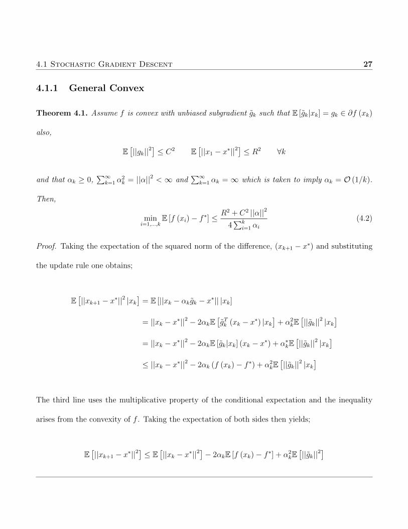
4.1.1 General Convex
Theorem 4.1. Assume f is convex with unbiased subgradient gk such that E [gk|xk] = gk ∈ ∂f (xk)
also,
E[||gk||2
]≤ C2 E
[||x1 − x∗||2
]≤ R2 ∀k
and that αk ≥ 0,∑∞
k=1 α2k = ||α||2 < ∞ and
∑∞k=1 αk = ∞ which is taken to imply αk = O (1/k).
Then,
mini=1,...,k
E [f (xi)− f ∗] ≤R2 + C2 ||α||2
4∑k
i=1 αi(4.2)
Proof. Taking the expectation of the squared norm of the difference, (xk+1 − x∗) and substituting
the update rule one obtains;
E[||xk+1 − x∗||2 |xk
]= E [||xk − αkgk − x∗|| |xk]
= ||xk − x∗||2 − 2αkE[gTk (xk − x∗) |xk
]+ α2
kE[||gk||2 |xk
]= ||xk − x∗||2 − 2αkE [gk|xk] (xk − x∗) + α∗kE
[||gk||2 |xk
]≤ ||xk − x∗||2 − 2αk (f (xk)− f ∗) + α2
kE[||gk||2 |xk
]
The third line uses the multiplicative property of the conditional expectation and the inequality
arises from the convexity of f . Taking the expectation of both sides then yields;
E[||xk+1 − x∗||2
]≤ E
[||xk − x∗||2
]− 2αkE [f (xk)− f ∗] + α2
kE[||gk||2
]
4.1 Stochastic Gradient Descent 28
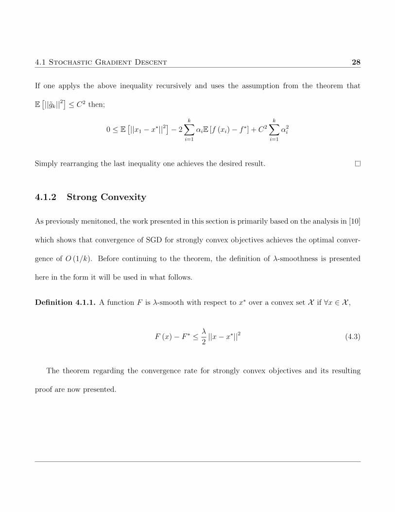
If one applys the above inequality recursively and uses the assumption from the theorem that
E[||gk||2
]≤ C2 then;
0 ≤ E[||x1 − x∗||2
]− 2
k∑i=1
αiE [f (xi)− f ∗] + C2
k∑i=1
α2i
Simply rearranging the last inequality one achieves the desired result.
4.1.2 Strong Convexity
As previously menitoned, the work presented in this section is primarily based on the analysis in [10]
which shows that convergence of SGD for strongly convex objectives achieves the optimal conver-
gence of O (1/k). Before continuing to the theorem, the definition of λ-smoothness is presented
here in the form it will be used in what follows.
Definition 4.1.1. A function F is λ-smooth with respect to x∗ over a convex set X if ∀x ∈ X ,
F (x)− F ∗ ≤ λ
2||x− x∗||2 (4.3)
The theorem regarding the convergence rate for strongly convex objectives and its resulting
proof are now presented.
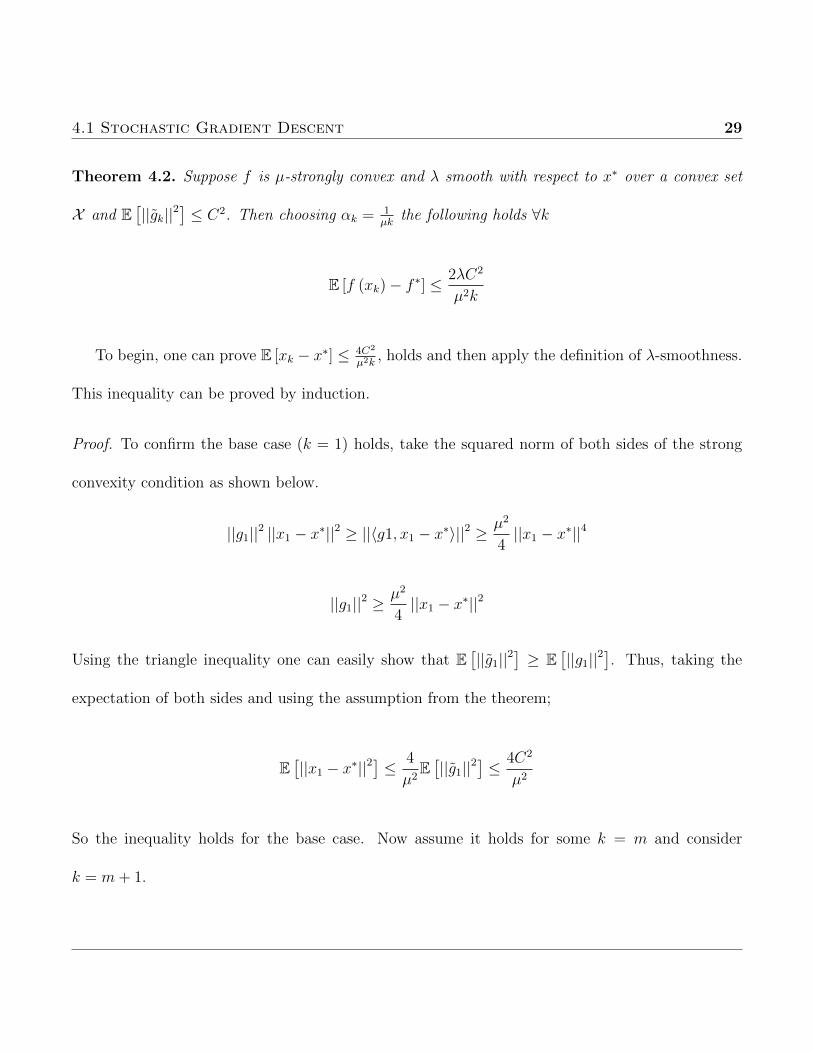
4.1 Stochastic Gradient Descent 29
Theorem 4.2. Suppose f is µ-strongly convex and λ smooth with respect to x∗ over a convex set
X and E[||gk||2
]≤ C2. Then choosing αk = 1
µkthe following holds ∀k
E [f (xk)− f ∗] ≤2λC2
µ2k
To begin, one can prove E [xk − x∗] ≤ 4C2
µ2k, holds and then apply the definition of λ-smoothness.
This inequality can be proved by induction.
Proof. To confirm the base case (k = 1) holds, take the squared norm of both sides of the strong
convexity condition as shown below.
||g1||2 ||x1 − x∗||2 ≥ ||〈g1, x1 − x∗〉||2 ≥µ2
4||x1 − x∗||4
||g1||2 ≥µ2
4||x1 − x∗||2
Using the triangle inequality one can easily show that E[||g1||2
]≥ E
[||g1||2
]. Thus, taking the
expectation of both sides and using the assumption from the theorem;
E[||x1 − x∗||2
]≤ 4
µ2E[||g1||2
]≤ 4C2
µ2
So the inequality holds for the base case. Now assume it holds for some k = m and consider
k = m+ 1.
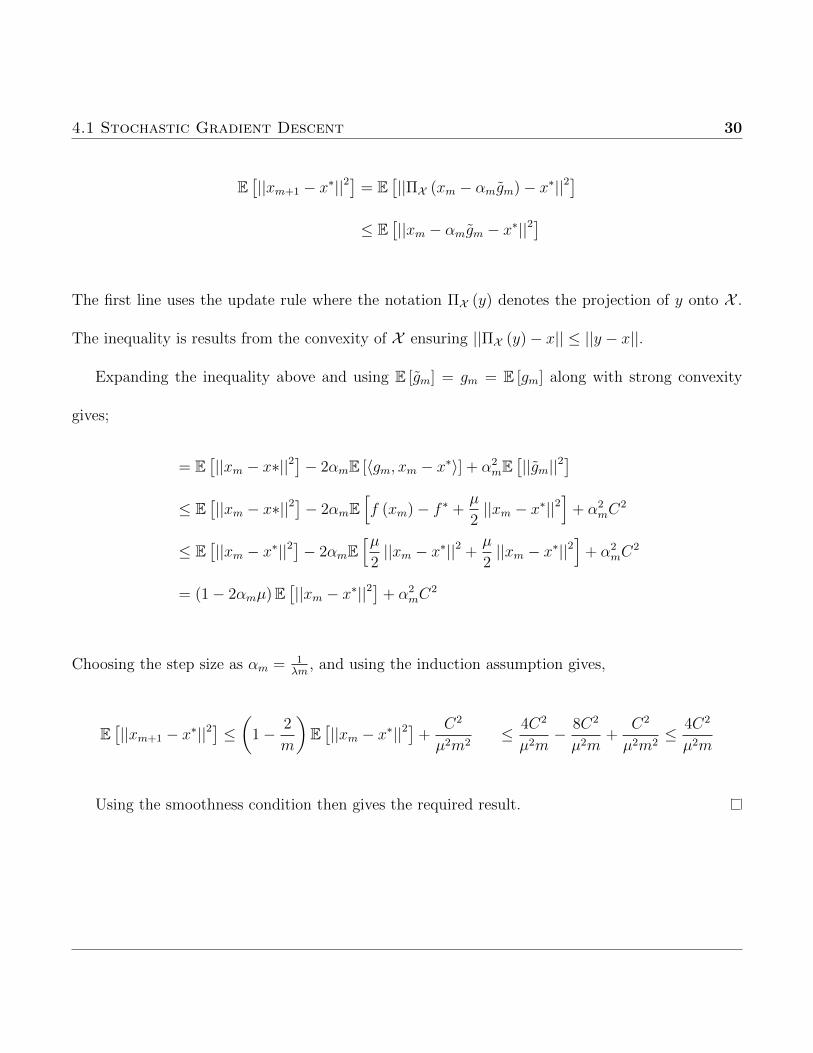
4.1 Stochastic Gradient Descent 30
E[||xm+1 − x∗||2
]= E
[||ΠX (xm − αmgm)− x∗||2
]≤ E
[||xm − αmgm − x∗||2
]
The first line uses the update rule where the notation ΠX (y) denotes the projection of y onto X .
The inequality is results from the convexity of X ensuring ||ΠX (y)− x|| ≤ ||y − x||.
Expanding the inequality above and using E [gm] = gm = E [gm] along with strong convexity
gives;
= E[||xm − x∗||2
]− 2αmE [〈gm, xm − x∗〉] + α2
mE[||gm||2
]≤ E
[||xm − x∗||2
]− 2αmE
[f (xm)− f ∗ +
µ
2||xm − x∗||2
]+ α2
mC2
≤ E[||xm − x∗||2
]− 2αmE
[µ2||xm − x∗||2 +
µ
2||xm − x∗||2
]+ α2
mC2
= (1− 2αmµ)E[||xm − x∗||2
]+ α2
mC2
Choosing the step size as αm = 1λm
, and using the induction assumption gives,
E[||xm+1 − x∗||2
]≤(
1− 2
m
)E[||xm − x∗||2
]+
C2
µ2m2≤ 4C2
µ2m− 8C2
µ2m+
C2
µ2m2≤ 4C2
µ2m
Using the smoothness condition then gives the required result.
4.2 Randomized Coordinate Gradient Descent 31
4.2 Randomized Coordinate Gradient Descent
The convergence analysis to be discussed in the two subsequent sections is prominently based on
work done by Nesterov in [3]. As suggested by the name, Randomized Coordinate Descent (RCD)
and its accelerated counterpart (ARCD) are applied coordinate-wise on the objective. Rather than
updating all parameters using a random subgradient, coordinate descent methods select a dimension
of the gradient and descend only in that direction during the current iteration. Thus, a general
form of the k + 1 iterate of this process is
xik+1= xik − αk∇fik (xk) (4.4)
Here, ik denotes the ith corrdinate of the kth iteration. Due to the clear depenedence on
corrdinate-wise operations of RCGD a definition of Lipschitz continuity that fits this setting will
be quite useful.
Definition 4.2.1. Coordinate-wise Lipschitz continuity A function f : Rd → R has coordinate-wise
Lipschitz continuous gradient with respect to coordinate i if
‖f ′i (x+ αei)− fi (x) ‖ ≤ Li‖αei‖, (4.5)
or equivalently
f (x+ αei) ≤ f (x) + α〈f ′i (x) , ei〉+αLi
2‖ei‖2 (4.6)
f (x)− f (yi) ≥1
2Li‖f ′i (x) ‖2 (4.7)
where yi (x) = x− 1Lif ′i (x).
4.2 Randomized Coordinate Gradient Descent 32
In [3] a random counter Rα, α ∈ R is defined which generates an integer i ∈ {1, . . . , n} with
probability that depends on the probability distribution assigned by α. For simplicity, α = 0 is the
distribution considered and corresponds to a uniform distribution. The random variable associated
to the sequence of integers is denoted as ξk = {i0, . . . , ik} and the expected value is written as
φk = Eξk−1f (xk).
Algorithm 5: RCD: Randomized Coordinate Descent
Data: x0: Initial parameter vectorinitialization;while xk not converged do
k → k + 1;ik → R0 (Randomly select coordinate to ”descend”);xk+1 → xk − 1
LikUikf
′ik
(xk) (Update parameters)
endResult: xk (Resulting parameters)
Access to coordinate-wise Lipschitz constants is usually not available, instead a constant time
step is used in practice which is equivalent to replacing Lik with an upper bound on all Lipschitz
factors.
4.2.1 General Convexity
Theorem 4.3. For f : Rd → R convex, with coordinate-wise Lipschitz continuous gradient and a
non-empty solution set the RCD method converges in the following manner for any k ≥ 0.
φk − f ∗ ≤2n
k + 4R2
1 (x0) , (4.8)
where R1 (x0) = maxx{maxx∗∈χ∗ ‖x− x∗‖1 : f (x) ≤ f (x0)}.
4.2 Randomized Coordinate Gradient Descent 33
Proof. If a sequence of integers ik is generated by the RCD method then
f (xk)− Eik (f (xk+1)) = Eik [f (xk)− f (xk+1)]
=n∑i=1
p(i) · [f (xk)− f (Ti (xk))]
≥n∑i=1
p(i)
2Li‖f ′i (xk) ‖21 =
1
2n‖∇f (xk) ‖21 (4.9)
where p(i) denotes the probability of occurrence for each ik. The first inequality is due to cooredinate-
wise Lipschitz continuity and the last line is a result of the probability distribution being uniform.
Now, by convexity, the Cauchy Schwarz inequality and f (xk) ≤ f (x0) one has
f (xk)− f ∗ ≤ 〈∇f (xk) , xk − x∗〉 ≤ ‖∇f (xk) ‖1R1 (x0) , (4.10)
substituting this inequality into previous expression yields,
f (xk)− Eik (f (xk+1)) ≥1
2nR21 (x0)
(f (xk)− f ∗)2 . (4.11)
Take the expectation of both sides with respect to ξk−1
φk − φk+1 ≥1
2nR21 (x0)
Eξk−1
[(f (xk)− f ∗)2
]≥ 1
2nR21 (x0)
(φk − f ∗)2 .
This implies the following
1
φk+1 − f ∗− 1
φk − f ∗=
φk − φk+1
(φk+1 − f ∗) (φk − f ∗)≥ φk − φk+1
(φk − f ∗)2≥ 1
2nR21 (x0)
. (4.12)
Applying this relation recursively and noting that φ0 = f (x0) and f (x0)− f ∗ ≤ 12n‖x0 − x∗‖21,
1
φk − f ∗≥ 1
φ0 − f ∗+
k
2nR21 (x0)
≥ k + 4
2nR21 (x0)
(4.13)
4.2 Randomized Coordinate Gradient Descent 34
4.2.2 Strong Convexity
The strongly convex case is very much related to general convexity. The difference between the two
is similar to the difference between strong and weak convexity for gradient descent. For this reason
the analysis begins from an inequality shown for weak convexity as mentioned in the proof.
Theorem 4.4. Let f : Rd → R be strongly convex with convexity parameter µ > 0, have coordinate-
wise Lipschitz continuous gradient and non-empty solution set. Then RCD satisfies the convergence
relation
φk − f ∗ ≤(
1− µ
n
)k(f (x0)− f ∗) (4.14)
Proof. The first inequality below is do to equation 4.9 from the weak convex case. To obtain a
tighter bound use the strong convexity condition f (xk)− f ∗ ≤ 12µ‖∇f (xk) ‖2.
f (xk)− E [f (xk+1)] ≥1
2n‖∇f (xk) ‖21 ≥
µ
n(f (xk)− f ∗)
Take the expectation with respect to ξk+1 and subtract f ∗ frm both sides.
φk+1 − f ∗ ≤(
1− µ
n
)(φk − f ∗)
φk − f ∗ ≤(
1− µ
n
)k(φ0 − f ∗) =
(1− µ
n
)k(f (x0)− f ∗) (4.15)
The last line arises from applying the first line recursively.
4.3 Accelerated Randomized Coordinate Gradient Descent 35
4.3 Accelerated Randomized Coordinate Gradient Descent
As one may deduce, the difference between RCGD and ARCD is anagolous to the difference between
gradient descent and NAG. Transitioning from RCGD requires adding momentum to the algorithm
in the same manner as in Nesterov’s original accelerated gradient method. Notice however that
accelerating RCD forces the method of estimate sequences, originally proposed in [1], to appear in
the algorithm. Convergence of NAG in the strongly convex case was proved to converge without
such a technique in [9], however it requires using discretized Lyapunov functions which are not
accessible in the stochastic domain. The iterative scheme is essentially contained in Algorithm 6
through the computation of yk, vk+1 and xk+1.
A final note on notation used in [3] is in order before proceeding to the algorithm. The symbol
s# is defined by
s# ∈ argmaxx
[〈s, x〉 − 1
2‖x‖2
]For large problems one need not restrict the selection to one single coordinate. Algorithm 6 includes
this case by considering a decomposition of Rd as done by [3].
Rd = ⊗ni=1Rni d =n∑i=1
ni
A partition of the unit matrix along with any vector x can be written as follows.
Id = (U1, . . . , Un) ∈ Rd×d x =n∑i=1
Uix(i) x(i) ∈ Rni Ui ∈ Rd×ni i = 1, . . . , n
The final piece needed is to define the optimal coordinate step, which is again defined in [3] as
Ti (x) = x− 1
LiUif
′i (x)#
4.3 Accelerated Randomized Coordinate Gradient Descent 36
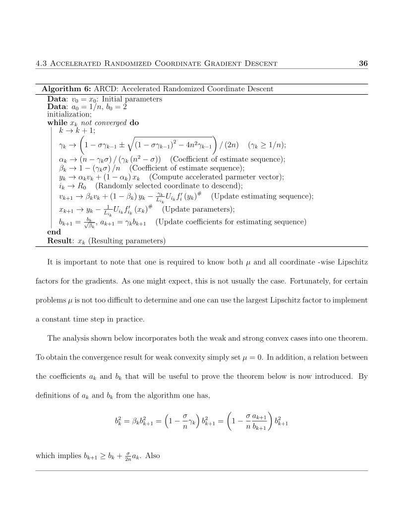
Algorithm 6: ARCD: Accelerated Randomized Coordinate Descent
Data: v0 = x0: Initial parametersData: a0 = 1/n, b0 = 2initialization;while xk not converged do
k → k + 1;
γk →(
1− σγk−1 ±√
(1− σγk−1)2 − 4n2γk−1
)/ (2n) (γk ≥ 1/n);
αk → (n− γkσ) / (γk (n2 − σ)) (Coefficient of estimate sequence);βk → 1− (γkσ) /n (Coefficient of estimate sequence);yk → αkvk + (1− αk)xk (Compute accelerated parmeter vector);ik → R0 (Randomly selected coordinate to descend);
vk+1 → βkvk + (1− βk) yk − γkLikUikf
′i (yk)
# (Update estimating sequence);
xk+1 → yk − 1LikUikf
′ik
(xk)# (Update parameters);
bk+1 = bk√βk
, ak+1 = γkbk+1 (Update coefficients for estimating sequence)
endResult: xk (Resulting parameters)
It is important to note that one is required to know both µ and all coordinate -wise Lipschitz
factors for the gradients. As one might expect, this is not usually the case. Fortunately, for certain
problems µ is not too difficult to determine and one can use the largest Lipschitz factor to implement
a constant time step in practice.
The analysis shown below incorporates both the weak and strong convex cases into one theorem.
To obtain the convergence result for weak convexity simply set µ = 0. In addition, a relation between
the coefficients ak and bk that will be useful to prove the theorem below is now introduced. By
definitions of ak and bk from the algorithm one has,
b2k = βkb2k+1 =
(1− σ
nγk
)b2k+1 =
(1− σ
n
ak+1
bk+1
)b2k+1
which implies bk+1 ≥ bk + σ2nak. Also
4.3 Accelerated Randomized Coordinate Gradient Descent 37
a2k+1
b2k+1
− ak+1
nbk+1
=βka
2k
b2k=
a2kb2k+1
,
similarly this leads to ak+1 ≥ ak + 12nbk. Now it is possible to prove by induction that
ak ≥1√σ
(Hk+1
1 −Hk+12
)bk ≥ Hk+1
1 +Hk+12 ,
where H1 = 1 +√σ
2nand H2 = 1−
√σ
2n.
Obviously these relations hold for k = 0 by the definitions given in the algorithm. Now assume
they hold for k = m and prove they hold true for k = m+ 1.
am+1 ≥ am +1
2nbm =
1√σ
(Hm+1
1 −Hm+12
)+
1√σ
(Hm+1
1 −Hm+12
)=
1√σ
(Hm+2
1 −Hm+22
)bm+1 ≥ bm +
σ
2nam = Hm+1
1 +Hm+12 +
σ
2n
1√σ
(Hm+1
1 −Hm+12
)= Hm+2
1 +Hm+22
Theorem 4.5. Let f : Rd → R have coordinate-wise Lipschitz continuous gradient, a non-empty
solution set and has convexity parameter µ ≥ 0. Then the ARCD method converges with the
following rate
φk − f ∗ ≤(
n
k + 1
)2 [2‖x0 − x∗‖2 +
1
n2(f (x0)− f ∗)
](4.16)
Proof. Assume xk and vk are the implementations of corresponding random variables generated by
ARCD. Let
r2k = ‖vk − x∗‖21 vk = yk +1− αkαk
(yk − xk) ,
where yk is defined by the ARCD algorithm. Then consider
4.3 Accelerated Randomized Coordinate Gradient Descent 38
r2k+1 = ‖βkvk + (1− βk) yk −γkLik
Uikf′i (yk)− x∗‖2
= ‖βkvk + (1− βk) yk − x∗‖21 +γ2kLik‖fik (yk) ‖2ik +
2γkLik〈f ′ik (yk) , (x
∗ − βkvk − (1− βk) yk)(ik)〉
≤ ‖βkvk + (1− βk) yk − x∗‖21 + 2γ2k (f (yk)− f (Tik (yk)))
+2γk〈f ′ik (yk) ,
(x∗ − yk +
βk (1− αk)αk
(xk − yk))(ik)
〉
The last equality arises by replacing the 1-norm with the norm with respect to the random variable
ik. The final line is a result of the convexity condition noted at the beginning of the RCD section.
Taking the expectation with respect to ik and then using the strong convexity condition gives,
Eik[r2k+1
]≤ βkr
2k + (1− βk) ‖yk − x∗‖21 + 2γ2k (f (yk)− Eik [f (xk+1)])
+2γkn〉∇f (yk) , x
∗ − yk +βk (1− αk)
αk(xk − yk)〉
≤ β2kr
2k + (1− βk) ‖yk − x∗‖2 + 2γ2k (f (yk)− Eik [f (xk=1)])
+2γkn
[f ∗ − f (yk)−
µ
2‖yk − x∗‖21 +
βk (1− αk)αk
(f (xk)− f (yk))
]
Eik[r2k+1
]= βkr
2k − 2γ2kEik [f (xk+1)] +
(1− βk −
µγkn
)‖yk − x∗‖21
+
(2γ2k −
2γkn
+2γkn
βk (1− αk)αk
)f (yk) +
2γkn
[f ∗ +
βk (1− αk)αk
f (xk)
]= βkr
2k − 2γ2kEik [f (xk+1)] +
2γkn
(f ∗ +
βk (1− αk)αk
f (xk)
)
The last line is due to βk = 1 − σγkn
, γ2k −γkn
= βkγk(1−αk)nαk
, both of which can be derived from the
algorithm. Also from the algorithm
4.4 ADAM 39
b2k+1 =b2kβk, a2k+1 = γ2kb
2k+1,
a2kb2k+1
=γkβk (1− αk)
nαk.
Using these relations, multiply both sides of the previous inequality by b2k+1 and take the expectation
in ξk−1.
b2k+1Eik[r2k+1
]≤ b2kr
2k − 2a2k+1 (Eik [f (xk+1)]− f ∗) + 2a2k (f (xk)− f ∗)
2a2k+1 (φk+1 − f ∗) ≤ 2a2k (φk − f ∗) + b2kr2k
≤ 2a20 (f (x0)− f ∗) + b20‖x0 − x∗‖21
Using the relation between a2k+1,a20 and b20 at the beginning of the section the expected convergence
result is easily obtained.
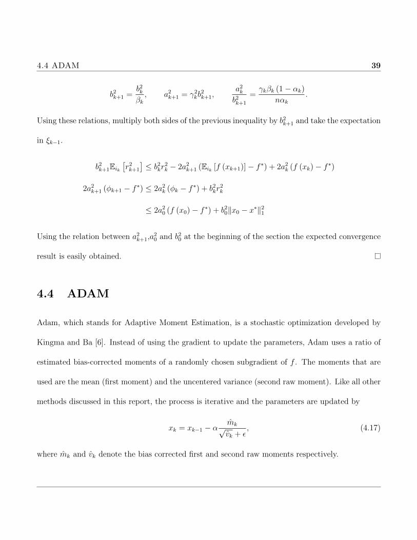
4.4 ADAM
Adam, which stands for Adaptive Moment Estimation, is a stochastic optimization developed by
Kingma and Ba [6]. Instead of using the gradient to update the parameters, Adam uses a ratio of
estimated bias-corrected moments of a randomly chosen subgradient of f . The moments that are
used are the mean (first moment) and the uncentered variance (second raw moment). Like all other
methods discussed in this report, the process is iterative and the parameters are updated by
xk = xk−1 − αmk√vk + ε
, (4.17)
where mk and vk denote the bias corrected first and second raw moments respectively.
4.4 ADAM 40
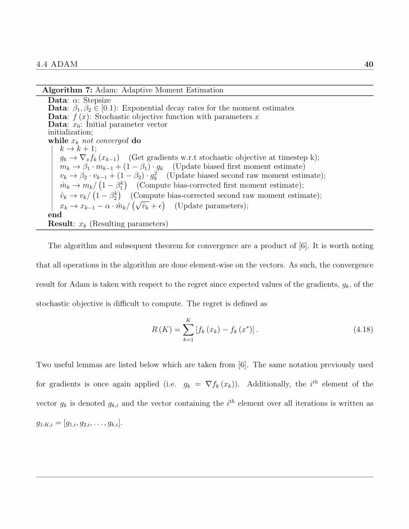
Algorithm 7: Adam: Adaptive Moment Estimation
Data: α: StepsizeData: β1, β2 ∈ [0.1): Exponential decay rates for the moment estimatesData: f (x): Stochastic objective function with parameters xData: x0: Initial parameter vectorinitialization;while xk not converged do
k → k + 1;gk → ∇xfk (xk−1) (Get gradients w.r.t stochastic objective at timestep k);mk → β1 ·mk−1 + (1− β1) · gk (Update biased first moment estimate)vk → β2 · vk−1 + (1− β2) · g2k (Update biased second raw moment estimate);mk → mk/
(1− βk1
)(Compute bias-corrected first moment estimate);
vk → vk/(1− βk2
)(Compute bias-corrected second raw moment estimate);
xk → xk−1 − α · mk/(√
vk + ε)
(Update parameters);endResult: xk (Resulting parameters)
The algorithm and subsequent theorem for convergence are a product of [6]. It is worth noting
that all operations in the algorithm are done element-wise on the vectors. As such, the convergence
result for Adam is taken with respect to the regret since expected values of the gradients, gk, of the
stochastic objective is difficult to compute. The regret is defined as
R (K) =K∑k=1
[fk (xk)− fk (x∗)] . (4.18)
Two useful lemmas are listed below which are taken from [6]. The same notation previously used
for gradients is once again applied (i.e. gk = ∇fk (xk)). Additionally, the ith element of the
vector gk is denoted gk,i and the vector containing the ith element over all iterations is written as
g1:K,i = [g1,i, g2,i, . . . , gk,i].
4.4 ADAM 41
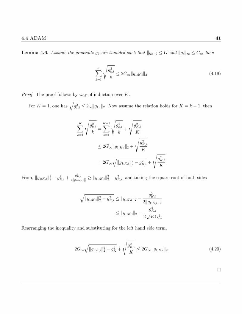
Lemma 4.6. Assume the gradients gk are bounded such that ‖gk‖2 ≤ G and ‖gt‖∞ ≤ G∞ then
K∑k=1
√g2k,ik≤ 2G∞‖g1:K,i‖2 (4.19)
Proof. The proof follows by way of induction over K.
For K = 1, one has√g21,i ≤ 2∞‖g1,i‖2. Now assume the relation holds for K = k − 1, then
K∑k=1
√g2k,ik
=K−1∑k=1
√g2k,ik
+
√g2K,iK
≤ 2G∞‖g1:K,i‖2 +
√g2K,iK
= 2G∞
√‖g1:K,i‖22 − g2K,i +
√g2K,iK
From, ‖g1:K,i‖22 − g2K,i +g4K,i
4‖g1:K,i‖22≥ ‖g1:K,i‖22 − g2K,i, and taking the square root of both sides
√‖g1:K,i‖22 − g2K,i ≤ ‖g1:T,i‖2 −
g2K,i2‖g1:K,i‖2
≤ ‖g1:K,i‖2 −g2K,i
2√KG2
∞
Rearranging the inequality and substituting for the left hand side term,
2G∞
√‖g1:K,i‖22 − g2K +
√g2K,iK≤ 2G∞‖g1:K,i‖2 (4.20)
4.4 ADAM 42
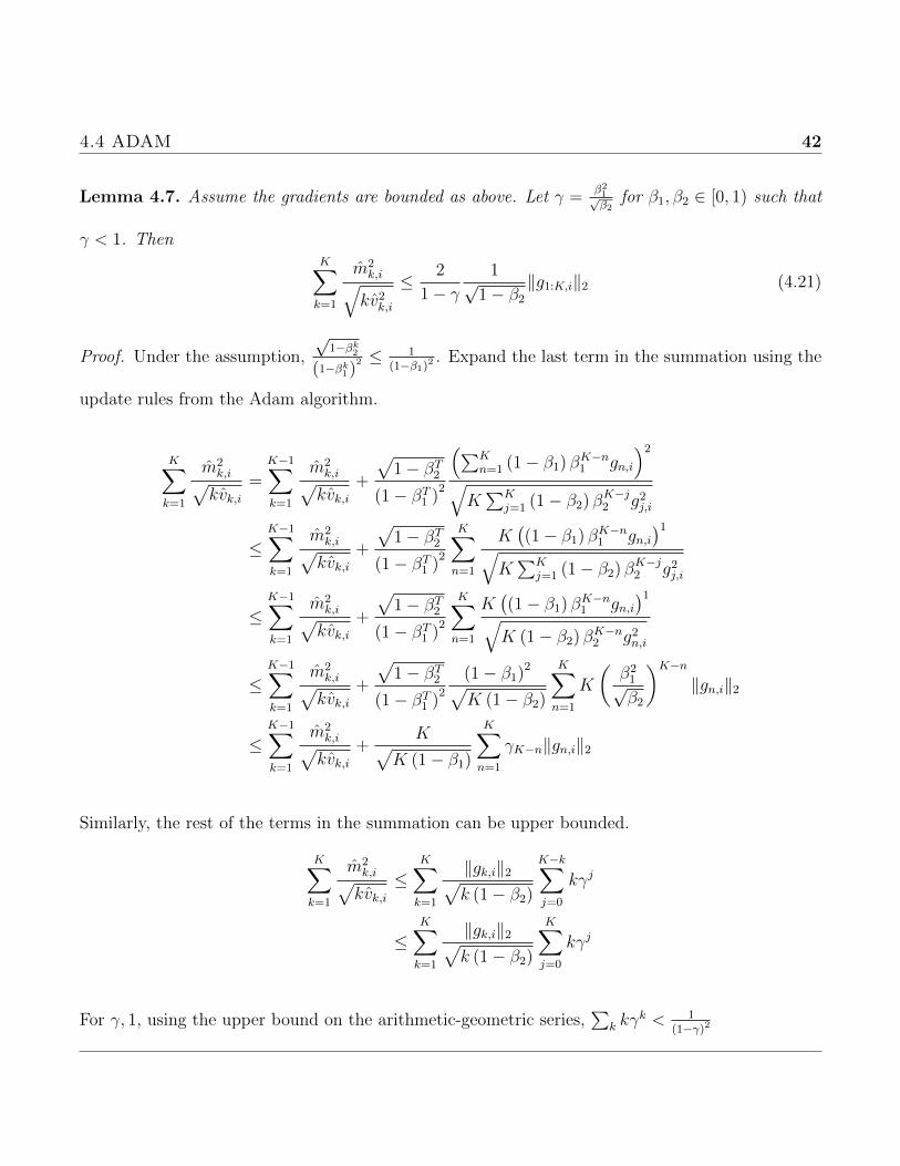
Lemma 4.7. Assume the gradients are bounded as above. Let γ =β21√β2
for β1, β2 ∈ [0, 1) such that
γ < 1. ThenK∑k=1
m2k,i√kv2k,i
≤ 2
1− γ1√
1− β2‖g1:K,i‖2 (4.21)
Proof. Under the assumption,
√1−βk
2
(1−βk1)
2 ≤ 1(1−β1)2
. Expand the last term in the summation using the
update rules from the Adam algorithm.
K∑k=1
m2k,i√kvk,i
=K−1∑k=1
m2k,i√kvk,i
+
√1− βT2
(1− βT1 )2
(∑Kn=1 (1− β1) βK−n1 gn,i
)2√K∑K
j=1 (1− β2) βK−j2 g2j,i
≤K−1∑k=1
m2k,i√kvk,i
+
√1− βT2
(1− βT1 )2
K∑n=1
K((1− β1) βK−n1 gn,i
)1√K∑K
j=1 (1− β2) βK−j2 g2j,i
≤K−1∑k=1
m2k,i√kvk,i
+
√1− βT2
(1− βT1 )2
K∑n=1
K((1− β1) βK−n1 gn,i
)1√K (1− β2) βK−n2 g2n,i
≤K−1∑k=1
m2k,i√kvk,i
+
√1− βT2
(1− βT1 )2
(1− β1)2√K (1− β2)
K∑n=1
K
(β21√β2
)K−n‖gn,i‖2
≤K−1∑k=1
m2k,i√kvk,i
+K√
K (1− β1)
K∑n=1
γK−n‖gn,i‖2
Similarly, the rest of the terms in the summation can be upper bounded.
K∑k=1
m2k,i√kvk,i
≤K∑k=1
‖gk,i‖2√k (1− β2)
K−k∑j=0
kγj
≤K∑k=1
‖gk,i‖2√k (1− β2)
K∑j=0
kγj
For γ, 1, using the upper bound on the arithmetic-geometric series,∑
k kγk < 1
(1−γ)2
4.4 ADAM 43
K∑k=1
‖gk,i‖2√k (1− β2)
K∑j=0
kγj ≤ 1
(1− γ)2√
1− β2
K∑k=1
‖gk,i‖2√k
Applying Lemma 4.6 one obtains,
K∑k=1
m2k,i√kvk,i
≤ 2G∞
(1− γ)2√
1− β2‖g1:K,i‖2
Theorem 4.8. Assume fk has bounded gradients, ‖∇fk (x) ‖2 ≤ G, ‖∇fk (x) ‖∞ ≤ G∞ for all
x ∈ Rd and the distance between any xk generated by Adam is bounded, ‖xn − xm‖2 ≤ D, ‖xn −
xm‖∞ ≤ D∞ for any m,n ∈ {1, . . . , K} and β1, β2 ∈ [0, 1) saitsfy β1√β2
< 1. Let αk = αk√k
and
β1,k = β1λk−1,λ ∈ (0, 1). Adam achieves the following guarantee for all K ≥ 1.
R (K) ≤d∑i=1
[D2
2α (1− β1)√KvK,i +
α (β1 + 1)G∞
(1− β1)√
1− β2 (1− γ)2‖g1:K,i‖2 +
D2∞G∞
√1− β2
2α (1− β1) (1− λ)2
](4.22)
Proof. From the convexity of each fk one has,
fk (xk)− fk (x∗) ≤ gTk (xk − x∗) =d∑i=1
gk,i(xk,i − x∗,i
)Now, in its full form the Adam update rule can be written as
xk+1 = xk −αk
1− βk1
(β1,k√vkmk−1 −
(1− β1,k)√vk
gk
)
4.4 ADAM 44
Since all of the operation from the Adam algorithm are performed element-wise, the focus now lies
on the ith dimension of xk. From here subtract x∗,i from both sides of the update rule above and
then square the resulting equation. This gives,
(xk+1,i − x∗,i
)2=(xk,i − x∗,i
)2 − 2αk1− βk1
(β1,k√vkmk−1,i +
1− β1,k√vk,i
gk,i
)(xk,i − x∗,i
)+ α2
k
(mk,i√vt,i
)2
Since the goal is to analyze the regret, it makes sense to rearrange the above equation for gk,i(xk,i − x∗,i
).
An upper bound on the first relation below is available by assigning
a =
(β1,k√vk−1,i
αk (1− β1,k)
)1/2
·(x∗,i − xk,i
), b =
(β1,tαk−1
(1− β1,t)√vk−1,i
)1/2
mk−1,i,
and using the the inequality a2 + b2 ≥ 2ab.
gk,i(xk,i − x∗,i
)=
(1− βk1
)√vk,i
2αk (1− β1,k)
[(xk,i − x∗,i
)2 − (xk+1,i − x∗,i)2]
+ a · b+αk(1− βk1
)√vk,i
2 (1− β1,k)
(mk,i√vk,i
)2
≤ 1
2αk (1− β1)
[(xk,i − x∗,i
)2 − (xk+1,i − x,i)2]√
vk,i
+β1,k
2αk−1 (1− β1,k)(x∗,i − xk,i
)2√vk−1,i +
β1αk−12 (1− β1)
m2k−1,i√vk−1,i
+αk
2 (1− β1)m2k,i√vk,i
The regret can be found by using inequality from Lemma 4.7 and summing the previous inequality
over all dimensions (i.e. i = 1, . . . , d).
R (K) ≤d∑i=1
[1
2α1 (1− β1)(x1,i − x∗,i
)2√v1,i +
K∑k=2
1
2 (1− β1)(xk,i − x∗,i
)2(√vk,i
αk−√vk−1,i
αk−1
)]
+d∑i=1
[α (1 + β1)G∞
(1− β1)√
1− β2 (1− γ)2‖g1:K,i‖2 +
K∑k=1
β1,k2αk (1− β1,k)
(x∗,i − xk,i
)2√vk,i
]
4.4 ADAM 45
≤d∑i=1
[D2
2α (1− β1)√KvK,i +
α (1 + β1)G∞
(1− β1)√
1− β2 (1− γ)2‖g1:K,i‖2 +
D2∞
2α
k∑k=1
β1,k1− β1,k
√kvk,i
]
≤d∑i=1
[D2
2α (1− β1)√KvK,i +
α (1 + β1)G∞
(1− β1)√
1− β2 (1− γ)2‖g1:K,i‖2 +
D2∞G∞
√1− β2
2α
k∑k=1
β1,k1− β1,k
√k
]
The last inequality is due to the bound on the 2-norm and ∞-norm of the parameter vector. One
arrives at the final result once it is noticed that the final term is upper bounded as laid out below.
Remember β1,k = β1λk−1 for λ ∈ (0, 1).
k∑k=1
β1,k1− β1,k
√k ≤
k∑k=1
1
1− β1λk−1√k ≤
k∑k=1
1
1− β1λk−1t ≤ 1
(1− β1) (1− λ)2
This bound on the regret can be verified by numerical results in practice. However, to do so
would require keeping track of all iterations of the parameter vector and gradients which is not
practical when dealing with very large problems. This result simply shows that the regret for Adam
obeys a O(√
k)
bound [6]. In particular, the summation in the theorem can be bounded in a
stronger sense if the input data is sparse since g1:K,i and vK,i will expectedly be sparse and thus can
be bounded above by G∞.
4.5 AdaGrad 46
4.5 AdaGrad
Introduced in 2011 by Duchi et al [7], Adagrad is simple variant of Adam which is useful when
working with sparse gradients. When bias-correction is applied to Adam, as it was above, Adagrad
corresponds to β1 = 0 and β2 = 1− ε. This coincides to an update rule of
xk+1 = xk − αkgk√∑kj=1 g
2j
(4.23)
This update arises from taking the limit of vk from Adam as β2 approaches 1.
limβ2→1
vk = limβ2→1
(1− β2)(1− βk2
) k∑j=1
βk−j2 · g2j =1
k
k∑j=1
g2j (4.24)
Theorem 4.9. Assume the distance between any xk generated by Adagrad is bounded ‖xn−xm‖2 ≤
D,‖xn− xm‖∞ ≤ D∞ for any m,n ∈ {1, . . . , K}. Suppose f is convex with non-empty solution set,
then Adagrad achieves the following guarantee for all K ≥ 1 and αk = α√k
R (K) ≤ 1
2α
d∑i=1
√Kg21:K,i +
d∑i=1
K∑k=1
αk2
g2k,j√∑kj=1 g
2j,i
(4.25)
Proof. First note that convexity of f implies
fk (xk)− fk (x∗) ≤d∑i=1
gk,i(xk,i − x∗,i
)(4.26)
4.5 AdaGrad 47
Next subtract x∗,i from both sides of the update rule and square the inequality.
(xk+1,i − x∗,i
)2=(xk,i − x∗,i
)2 − 2αkgk.i√∑kj=1 g
2j,i
(xk,i − x∗,i
)+ α2
k
gk,i√∑kj=1 g
2j,i
2
By using the convexity condition given above, this equation can be rearranged to give the regret
by adding over all k = 1, . . . , K
gk,i(xk,i − x∗,i
)=
1
2αk
√√√√ k∑j=1
g2j,i
[(xk,i − x∗,i
)2 − (xk+1,i − x∗,i)2]
+αk2
g2k,i√∑kj=1 g
2j,i
R (K) ≤d∑i=1
√g21,i
2αi
(x1,i − x∗,i
)2+
d∑i=1
K∑k=2
1
2
(xk,i − x∗,i
)2√∑k
j=1 g2j,i
2αk−
√∑k−1j=1 g
2j,i
2αk−1
+
d∑i=1
K∑k=1
αk2
g2k,i√∑kj=1 g
2j,i
(4.27)
As with Adam, one would have to have access to all iterations of the parameter vector and the
gradients in order to verify the regret bound. For this reason, in the next section, which covers
several numerical examples, the convergence will be qualitatively compared to one another rather
than individually corroborated.
Chapter 5
Numerical Examples
This chapter will cover several numerical examples in the hopes of providing a pratical understanding
of the optimization algorithms discussed in previous chapters. We begin by investigating multiple
two-dimensional objective functions in order to illustrate aspects of the algorithms within a relatively
simple setting. Not all of these functions are convex over the domain being consider which leads to
inefficient convergence for some methods while displaying the flexiblility of others. The functions
chosen are motivated by a list of optimization test functions and datasets found in [11]. In particular,
test functions are categorized based on the shape of the surface they define; for example, Bowl-
shaped, plate-shaped and multiple local minima. These classifications were chosen to attempt to
portray varying degrees of difficulty in optimizing test functions.
5.1 Ball Shaped 49
5.1 Ball Shaped
5.1.1 Sum of Squares Function
This is one of the simplest function to optimize since it simply involves summing up the squares of all
elements of the input vector. It is clearly convex and in two dimensions and has a global minimum
f (x∗) = 0 at x∗ = [0 0]. The intended search domain for this example will be xi = [−5 5].
The function for an arbitrary number of dimensions is listed below, however only d = 2 will be
considered.
f (~x) =d∑i=1
ix2i (5.1)
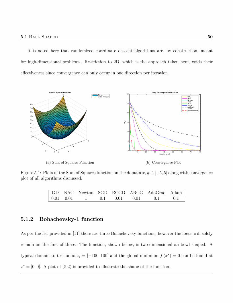
All discussed algorithms converge to the minimizer as expected. The purpose of including such
a simple test function is simply to ensure the supposed results a validated in a straightforward case.
The initial starting point was chosen as x0 = [−3,−3]. From 5.1(b), the first point to notice is
Newton converges in one iteration which is the predicted result. For NAG and GD it is challenging
to compare the actual rates of convergence (i.e. linear, quadratic) from 5.1(b) but the qualitatively
behaviour is the focus and in fact shows that NAG converges in less iterations than GD, which is
also the expected result.
Intuitively, SGD should converge more quickly than Adam or Adagrad since the SGD algorithm
allows for larger steps than Adagrad and Adam onvex functions. Namely, moment estimation tends
to under-estimate the magnitude of the subgradients for this test, hence when the three algorithms
use equivalent step sizes SGD will converge faster. Again this is the behaviour observed from 5.1(b).
5.1 Ball Shaped 50
It is noted here that randomized coordinate descent algorithms are, by construction, meant
for high-dimensional problems. Restriction to 2D, which is the approach taken here, voids their
effectiveness since convergence can only occur in one direction per iteration.
(a) Sum of Squares Function (b) Convergence Plot
Figure 5.1: Plots of the Sum of Squares function on the domain x, y ∈ [−5, 5] along with convergenceplot of all algorithms discussed.
GD NAG Newton SGD RCGD ARCG AdaGrad Adam0.01 0.01 1 0.1 0.01 0.01 0.1 0.1
5.1.2 Bohachevsky-1 function
As per the list provided in [11] there are three Bohachevsky functions, however the focus will solely
remain on the first of these. The function, shown below, is two-dimensional an bowl shaped. A
typical domain to test on is xi = [−100 100] and the global minimum f (x∗) = 0 can be found at
x∗ = [0 0]. A plot of (5.2) is provided to illustrate the shape of the function.

5.1 Ball Shaped 51
f (~x) = x21 + 2x22 − 0.3 cos (3πx1)− 0.4 cos (4πx2) + 0.7 (5.2)
As with the Sum of Squares function, all algorithms converge to the minimizer (with the excep-
tion of ARCG) assuming the step size is chosen small enough. The initial starting point for this
test was chosen as x0 = [−70, 70] simply due to symmetry, while x0 = [−15, 15] for Newton. In
terms of comparison, for the same time step GD and NAG converge as would be expected since
the function is convex. Newton requires more than one iteration this time since the function is not
quadratic. The stochastic methods appear to converge at a slower rate than the deterministic algo-
rithms for this test function, however choosing larger time steps for SGD, RCGD, and ARCG will
result in quicker convergence. Requiring such large step sizes for these convex functions suggests
that moment estimation is not as suitable for convergence in this scenario as simple deterministic
method would be. The step size values for each algorithm that were used for this test are given
below for reference as well.
(a) Bohachevsky Function (b) Convergence Plot
Figure 5.2: Plots of the Bohachevsky function on the domain x, y ∈ [−100, 100] along with conver-gence plot of all algorithms discussed.
5.2 Plate Shaped 52
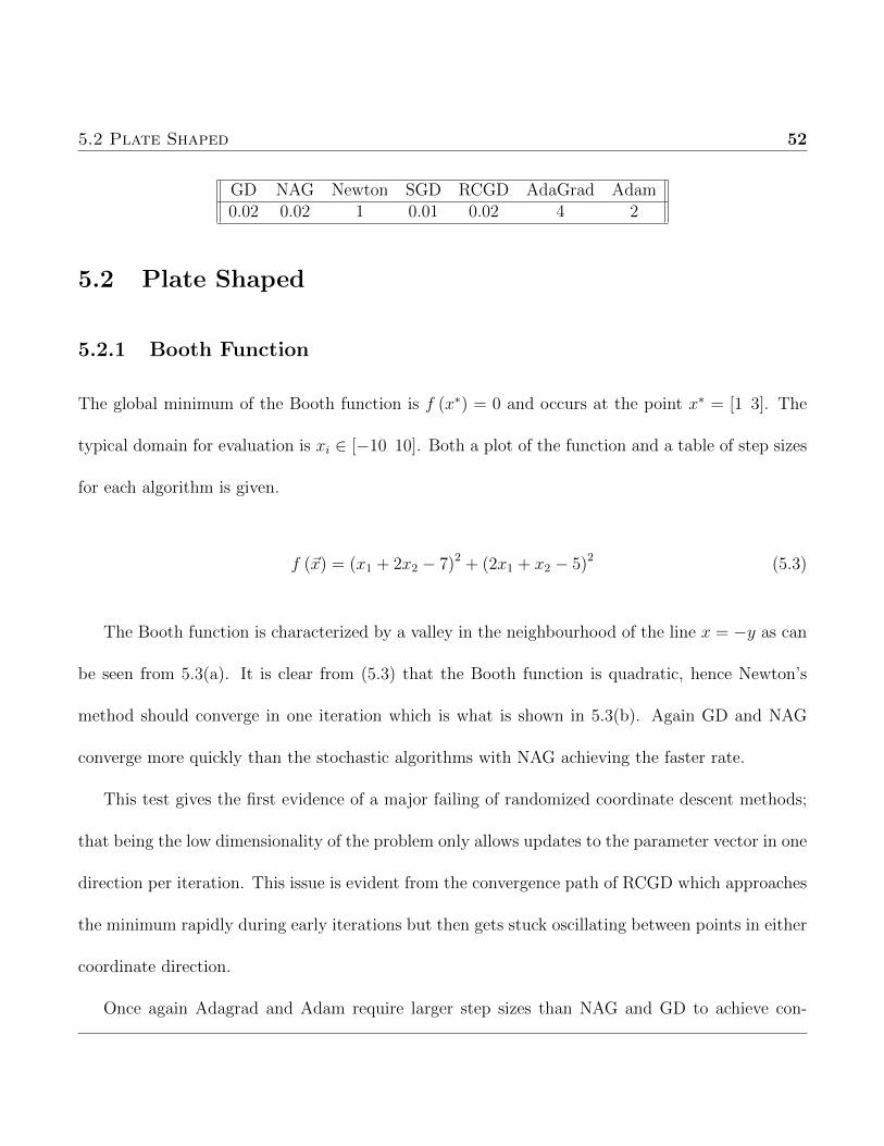
GD NAG Newton SGD RCGD AdaGrad Adam0.02 0.02 1 0.01 0.02 4 2
5.2 Plate Shaped
5.2.1 Booth Function
The global minimum of the Booth function is f (x∗) = 0 and occurs at the point x∗ = [1 3]. The
typical domain for evaluation is xi ∈ [−10 10]. Both a plot of the function and a table of step sizes
for each algorithm is given.
f (~x) = (x1 + 2x2 − 7)2 + (2x1 + x2 − 5)2 (5.3)
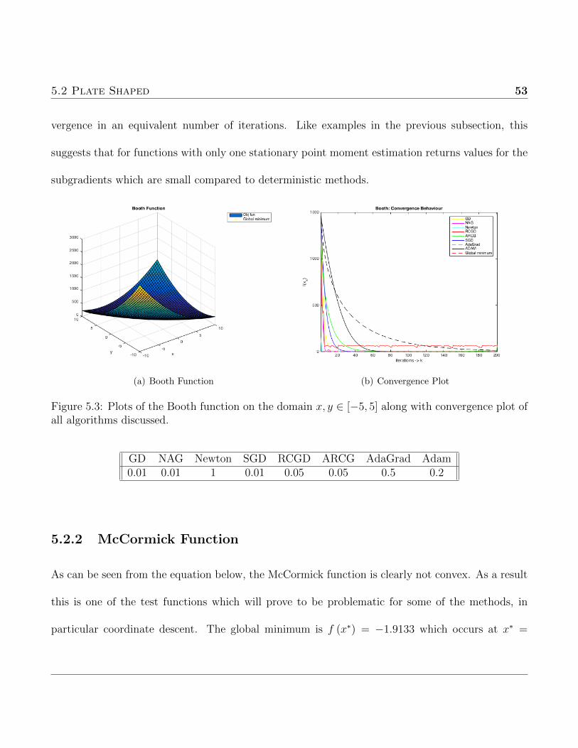
The Booth function is characterized by a valley in the neighbourhood of the line x = −y as can
be seen from 5.3(a). It is clear from (5.3) that the Booth function is quadratic, hence Newton’s
method should converge in one iteration which is what is shown in 5.3(b). Again GD and NAG
converge more quickly than the stochastic algorithms with NAG achieving the faster rate.
This test gives the first evidence of a major failing of randomized coordinate descent methods;
that being the low dimensionality of the problem only allows updates to the parameter vector in one
direction per iteration. This issue is evident from the convergence path of RCGD which approaches
the minimum rapidly during early iterations but then gets stuck oscillating between points in either
coordinate direction.
Once again Adagrad and Adam require larger step sizes than NAG and GD to achieve con-
5.2 Plate Shaped 53
vergence in an equivalent number of iterations. Like examples in the previous subsection, this
suggests that for functions with only one stationary point moment estimation returns values for the
subgradients which are small compared to deterministic methods.
(a) Booth Function (b) Convergence Plot
Figure 5.3: Plots of the Booth function on the domain x, y ∈ [−5, 5] along with convergence plot ofall algorithms discussed.
GD NAG Newton SGD RCGD ARCG AdaGrad Adam0.01 0.01 1 0.01 0.05 0.05 0.5 0.2
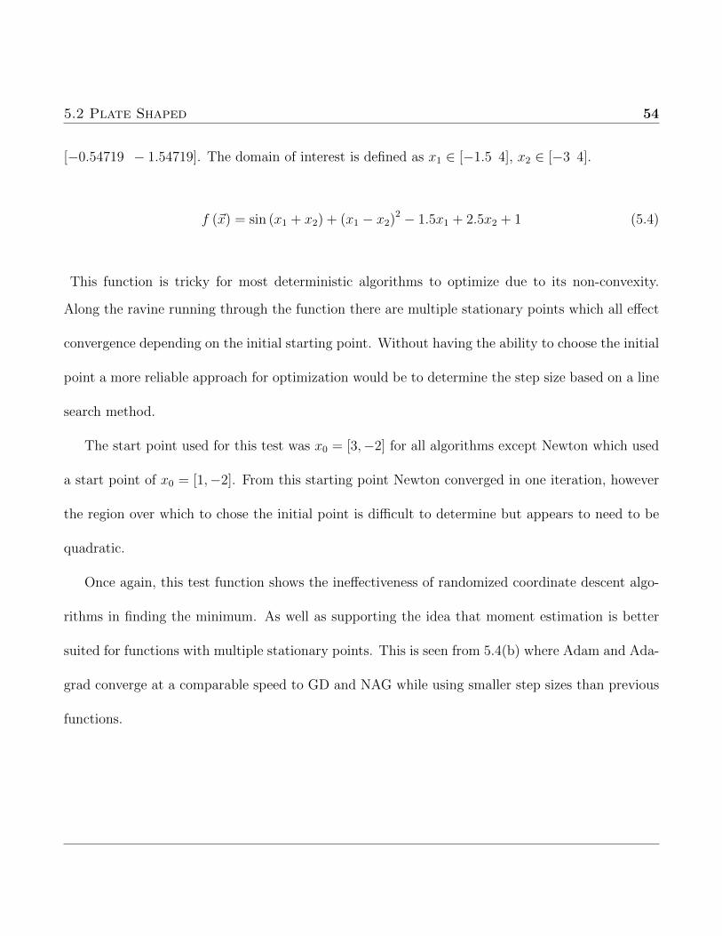
5.2.2 McCormick Function
As can be seen from the equation below, the McCormick function is clearly not convex. As a result
this is one of the test functions which will prove to be problematic for some of the methods, in
particular coordinate descent. The global minimum is f (x∗) = −1.9133 which occurs at x∗ =
5.2 Plate Shaped 54
[−0.54719 − 1.54719]. The domain of interest is defined as x1 ∈ [−1.5 4], x2 ∈ [−3 4].
f (~x) = sin (x1 + x2) + (x1 − x2)2 − 1.5x1 + 2.5x2 + 1 (5.4)
This function is tricky for most deterministic algorithms to optimize due to its non-convexity.
Along the ravine running through the function there are multiple stationary points which all effect
convergence depending on the initial starting point. Without having the ability to choose the initial
point a more reliable approach for optimization would be to determine the step size based on a line
search method.
The start point used for this test was x0 = [3,−2] for all algorithms except Newton which used
a start point of x0 = [1,−2]. From this starting point Newton converged in one iteration, however
the region over which to chose the initial point is difficult to determine but appears to need to be
quadratic.
Once again, this test function shows the ineffectiveness of randomized coordinate descent algo-
rithms in finding the minimum. As well as supporting the idea that moment estimation is better
suited for functions with multiple stationary points. This is seen from 5.4(b) where Adam and Ada-
grad converge at a comparable speed to GD and NAG while using smaller step sizes than previous
functions.
5.3 Functions with Many Local Minima 55
(a) McCormick Function (b) Convergence Plot
Figure 5.4: Plots of the McCormick function on the domain x, y ∈ [−5, 5] along with convergenceplot of all algorithms discussed.
GD NAG Newton SGD RCGD ARCG AdaGrad Adam0.01 0.01 1 0.1 0.001 0.001 0.4 0.2
5.3 Functions with Many Local Minima
5.3.1 Ackley Function
The Ackley function has a comparatively flat outer region but drops off quite drastically near the
global minimum f (~x) = 0 at x∗ = [0 0]. The test will be run on the domain xi = [−32.768 32.768]
with parameter values of a = 20, b = 0.2 and c = 2π. Notice that this function is also clearly not
convex over its domain. The purpose of testing this function is to better determine the flexibility
5.3 Functions with Many Local Minima 56
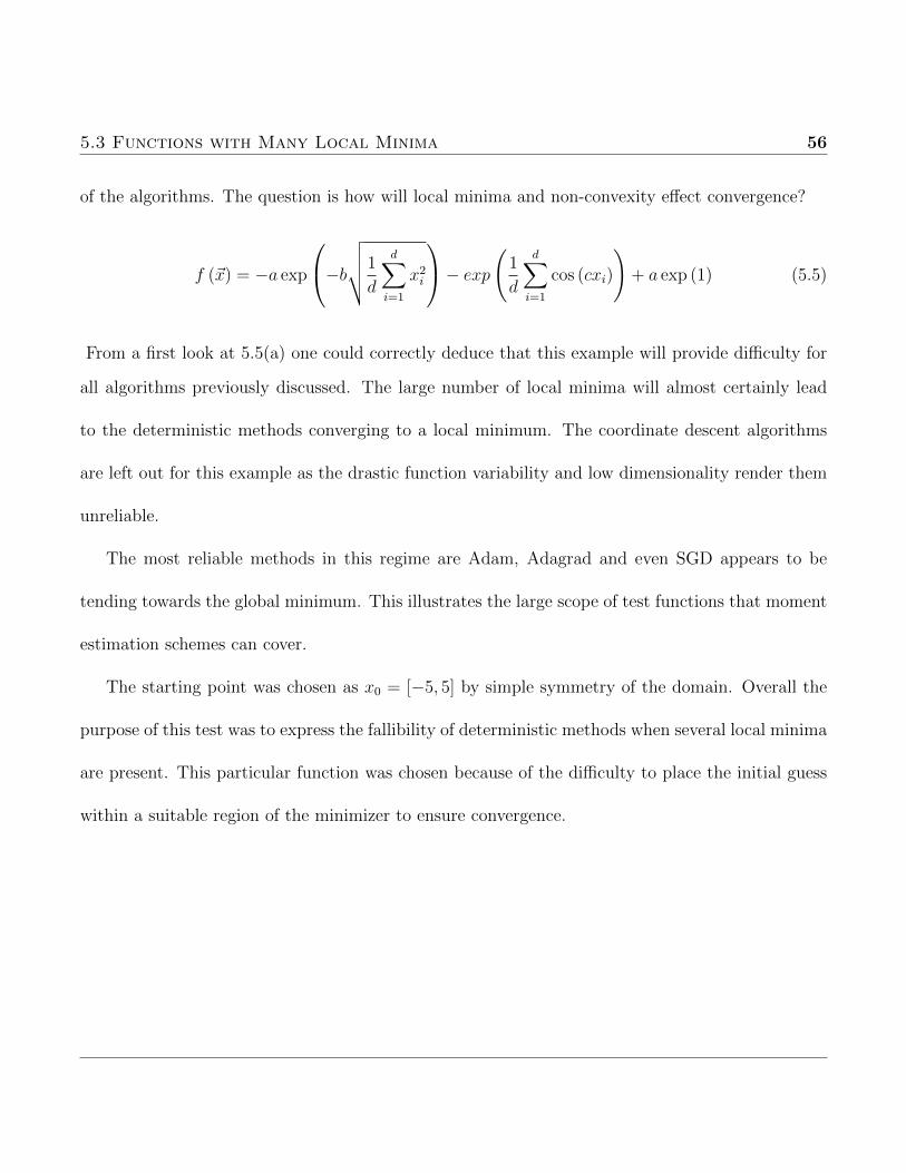
of the algorithms. The question is how will local minima and non-convexity effect convergence?
f (~x) = −a exp
−b√√√√1
d
d∑i=1
x2i
− exp(1
d
d∑i=1
cos (cxi)
)+ a exp (1) (5.5)
From a first look at 5.5(a) one could correctly deduce that this example will provide difficulty for
all algorithms previously discussed. The large number of local minima will almost certainly lead
to the deterministic methods converging to a local minimum. The coordinate descent algorithms
are left out for this example as the drastic function variability and low dimensionality render them
unreliable.
The most reliable methods in this regime are Adam, Adagrad and even SGD appears to be
tending towards the global minimum. This illustrates the large scope of test functions that moment
estimation schemes can cover.
The starting point was chosen as x0 = [−5, 5] by simple symmetry of the domain. Overall the
purpose of this test was to express the fallibility of deterministic methods when several local minima
are present. This particular function was chosen because of the difficulty to place the initial guess
within a suitable region of the minimizer to ensure convergence.
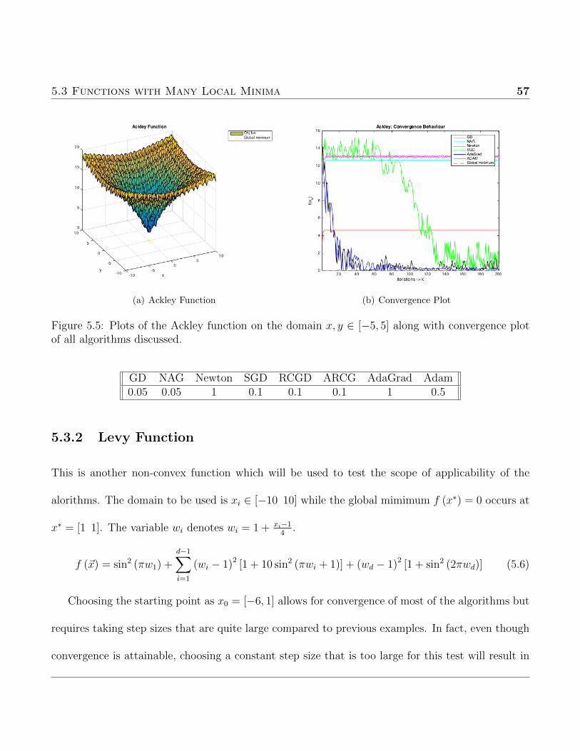
5.3 Functions with Many Local Minima 57
(a) Ackley Function (b) Convergence Plot
Figure 5.5: Plots of the Ackley function on the domain x, y ∈ [−5, 5] along with convergence plotof all algorithms discussed.
GD NAG Newton SGD RCGD ARCG AdaGrad Adam0.05 0.05 1 0.1 0.1 0.1 1 0.5
5.3.2 Levy Function
This is another non-convex function which will be used to test the scope of applicability of the
alorithms. The domain to be used is xi ∈ [−10 10] while the global mimimum f (x∗) = 0 occurs at
x∗ = [1 1]. The variable wi denotes wi = 1 + xi−14
.
f (~x) = sin2 (πw1) +d−1∑i=1
(wi − 1)2 [1 + 10 sin2 (πwi + 1)] + (wd − 1)2 [1 + sin2 (2πwd)] (5.6)
Choosing the starting point as x0 = [−6, 1] allows for convergence of most of the algorithms but
requires taking step sizes that are quite large compared to previous examples. In fact, even though
convergence is attainable, choosing a constant step size that is too large for this test will result in
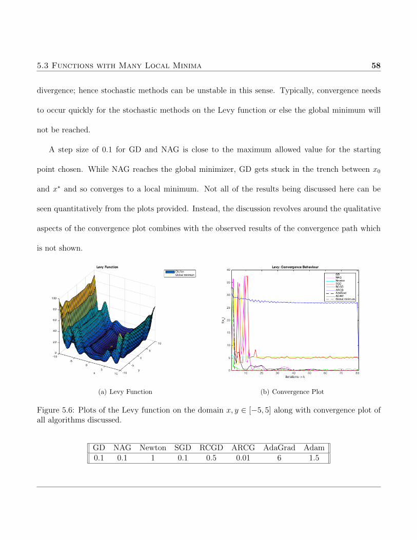
5.3 Functions with Many Local Minima 58
divergence; hence stochastic methods can be unstable in this sense. Typically, convergence needs
to occur quickly for the stochastic methods on the Levy function or else the global minimum will
not be reached.
A step size of 0.1 for GD and NAG is close to the maximum allowed value for the starting
point chosen. While NAG reaches the global minimizer, GD gets stuck in the trench between x0
and x∗ and so converges to a local minimum. Not all of the results being discussed here can be
seen quantitatively from the plots provided. Instead, the discussion revolves around the qualitative
aspects of the convergence plot combines with the observed results of the convergence path which
is not shown.
(a) Levy Function (b) Convergence Plot
Figure 5.6: Plots of the Levy function on the domain x, y ∈ [−5, 5] along with convergence plot ofall algorithms discussed.
GD NAG Newton SGD RCGD ARCG AdaGrad Adam0.1 0.1 1 0.1 0.5 0.01 6 1.5
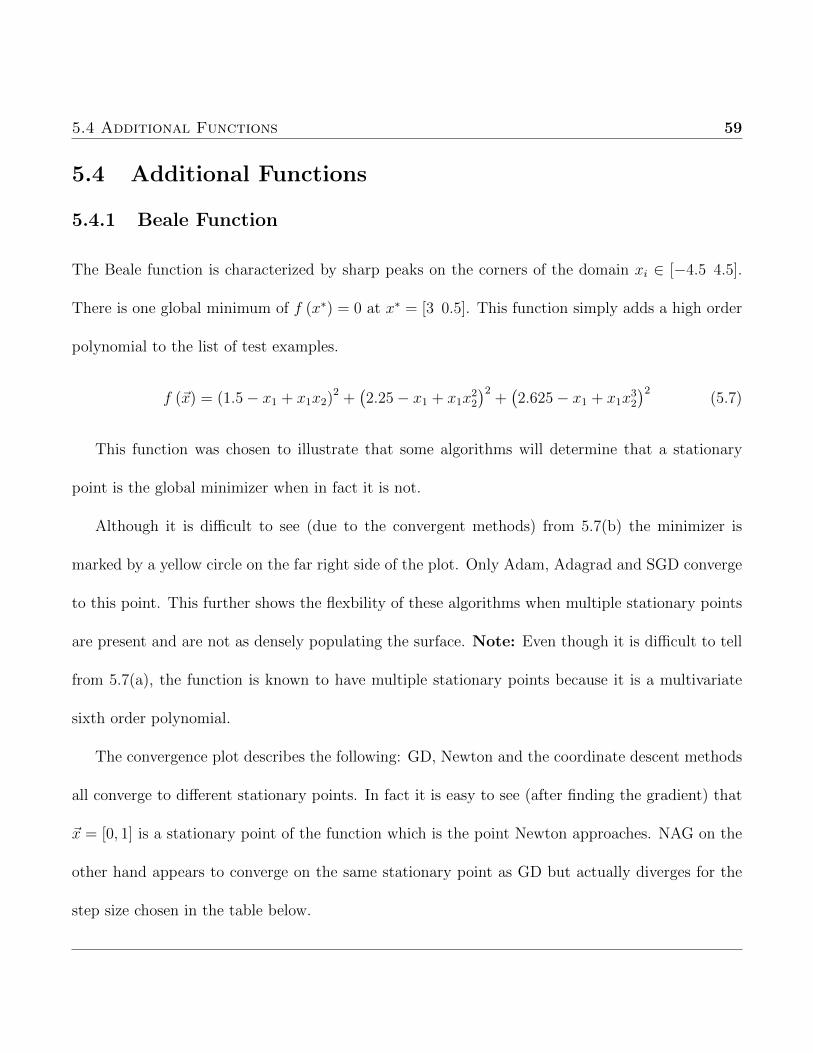
5.4 Additional Functions 59
5.4 Additional Functions
5.4.1 Beale Function
The Beale function is characterized by sharp peaks on the corners of the domain xi ∈ [−4.5 4.5].
There is one global minimum of f (x∗) = 0 at x∗ = [3 0.5]. This function simply adds a high order
polynomial to the list of test examples.
f (~x) = (1.5− x1 + x1x2)2 +
(2.25− x1 + x1x
22
)2+(2.625− x1 + x1x
32
)2(5.7)
This function was chosen to illustrate that some algorithms will determine that a stationary
point is the global minimizer when in fact it is not.
Although it is difficult to see (due to the convergent methods) from 5.7(b) the minimizer is
marked by a yellow circle on the far right side of the plot. Only Adam, Adagrad and SGD converge
to this point. This further shows the flexbility of these algorithms when multiple stationary points
are present and are not as densely populating the surface. Note: Even though it is difficult to tell
from 5.7(a), the function is known to have multiple stationary points because it is a multivariate
sixth order polynomial.
The convergence plot describes the following: GD, Newton and the coordinate descent methods
all converge to different stationary points. In fact it is easy to see (after finding the gradient) that
~x = [0, 1] is a stationary point of the function which is the point Newton approaches. NAG on the
other hand appears to converge on the same stationary point as GD but actually diverges for the
step size chosen in the table below.
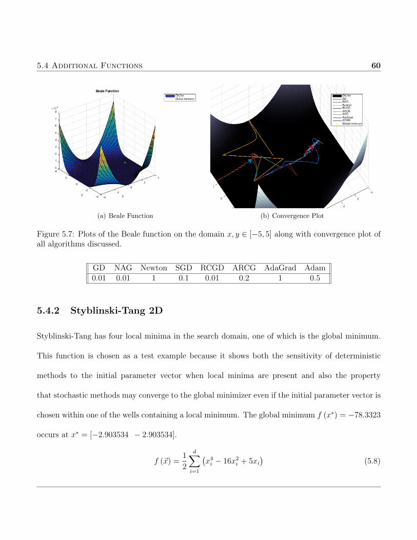
5.4 Additional Functions 60
(a) Beale Function (b) Convergence Plot
Figure 5.7: Plots of the Beale function on the domain x, y ∈ [−5, 5] along with convergence plot ofall algorithms discussed.
GD NAG Newton SGD RCGD ARCG AdaGrad Adam0.01 0.01 1 0.1 0.01 0.2 1 0.5
5.4.2 Styblinski-Tang 2D
Styblinski-Tang has four local minima in the search domain, one of which is the global minimum.
This function is chosen as a test example because it shows both the sensitivity of deterministic
methods to the initial parameter vector when local minima are present and also the property
that stochastic methods may converge to the global minimizer even if the initial parameter vector is
chosen within one of the wells containing a local minimum. The global minimum f (x∗) = −78.3323
occurs at x∗ = [−2.903534 − 2.903534].
f (~x) =1
2
d∑i=1
(x4i − 16x2i + 5xi
)(5.8)
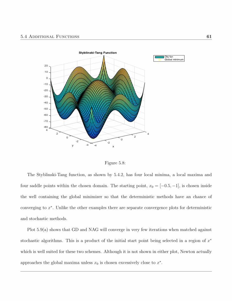
5.4 Additional Functions 61
Figure 5.8:
The Styblinski-Tang function, as shown by 5.4.2, has four local minima, a local maxima and
four saddle points within the chosen domain. The starting point, x0 = [−0.5,−1], is chosen inside
the well containing the global minimizer so that the deterministic methods have an chance of
converging to x∗. Unlike the other examples there are separate convergence plots for deterministic
and stochastic methods.
Plot 5.9(a) shows that GD and NAG will converge in very few iterations when matched against
stochastic algorithms. This is a product of the initial start point being selected in a region of x∗
which is well suited for these two schemes. Although it is not shown in either plot, Newton actually
approaches the global maxima unless x0 is chosen excessively close to x∗.
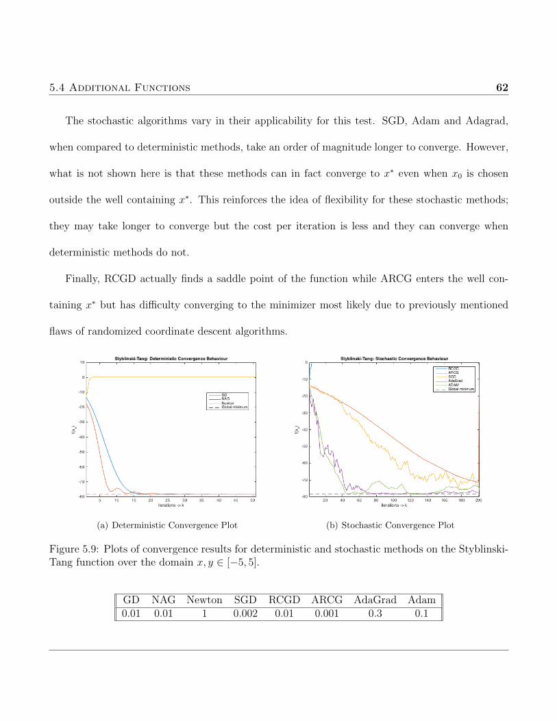
5.4 Additional Functions 62
The stochastic algorithms vary in their applicability for this test. SGD, Adam and Adagrad,
when compared to deterministic methods, take an order of magnitude longer to converge. However,
what is not shown here is that these methods can in fact converge to x∗ even when x0 is chosen
outside the well containing x∗. This reinforces the idea of flexibility for these stochastic methods;
they may take longer to converge but the cost per iteration is less and they can converge when
deterministic methods do not.
Finally, RCGD actually finds a saddle point of the function while ARCG enters the well con-
taining x∗ but has difficulty converging to the minimizer most likely due to previously mentioned
flaws of randomized coordinate descent algorithms.
(a) Deterministic Convergence Plot (b) Stochastic Convergence Plot
Figure 5.9: Plots of convergence results for deterministic and stochastic methods on the Styblinski-Tang function over the domain x, y ∈ [−5, 5].
GD NAG Newton SGD RCGD ARCG AdaGrad Adam0.01 0.01 1 0.002 0.01 0.001 0.3 0.1
Bibliography
[1] Yurii Nesterov. Introductory Lectures on Convex Optimization: A Basic Course, volume 87 of
Applied Optimization. Springer Science+Business Media New York, 2004.
[2] Yurii Nesterov. A method of solving a convex programming problem with convergence rate
o(1/k2). Soviet Mathematics Doklady, 27:372–376, 1983.
[3] Yurii Nesterov. Efficiency of coordinate descent methods on huge-scale optimization problems.
SIAM Journal on Optimization, 22:341–362, 2012.
[4] Z. Lu and L. Xiao. On the complexity analysis of randomized block-coordinate descent methods.
Mathematical Programming, 152:615–642, 2015.
[5] Qihang Lin, Zhaosong Lu, and Lin Xiao. An accelerated proximal coordinate gradient method.
In Z. Ghahramani, M. Welling, C. Cortes, N.d. Lawrence, and K.q. Weinberger, editors, Ad-
vances in Neural Information Processing Systems 27, pages 3059–3067. Curran Associates, Inc.,
2014.
BIBLIOGRAPHY 64
[6] Diederik P. Kingma and Jimmy Ba. Adam: A method for stochastic optimization. CoRR,
abs/1412.6980, 2014.
[7] John Duchi, Elad Hazan, and Yoram Singer. Adaptive subgradient methods for online learning
and stochastic optimization. J. Mach. Learn. Res., 12(1532-4435):2121–2159, July 2011.
[8] Ashia C. Wilson, Benjamin Recht, and Michael I. Jordan. A lyapunov analysis of momentum
methods in optimization. CoRR, abs/1611.02635, 2016.
[9] Weijie Su, Stephen Boyd, and Emmanuel J. Candes. A differential equation for modeling
nesterov’s gradient method: Theory and insights. J. Mach. Learn. Res., 17:1–43, September
2016.
[10] Alexander Rakhlin and Ohad Shamir. Making gradient descent optimal for strongly convex
stochastic optimization. CoRR, 2011.
[11] Derek Bingham and Sonja Surjanovic. Virtual library of simulation experiments: Test functions
and datasets, 2015. [Online; accessed July-2017].