Convection Heat Transfer

Reading Problems12-1→ 12-8 12-41, 12-48, 12-53, 12-68, 12-74, 12-78, 12-8113-1→ 13-6 13-39, 13-47, 13-5514-1→ 14-4 14-19, 14-25, 14-42, 14-48

Introduction

• the controlling equation for convection is Newton’s Law of Cooling

Qconv =∆T

Rconv

= hA(Tw − T∞) ⇒ Rconv =1

hA

A = total convective area, m2

h = heat transfer coefficient, W/(m2 ·K)

Tw = surface temperature, ◦C

T∞ = fluid temperature, ◦C

1

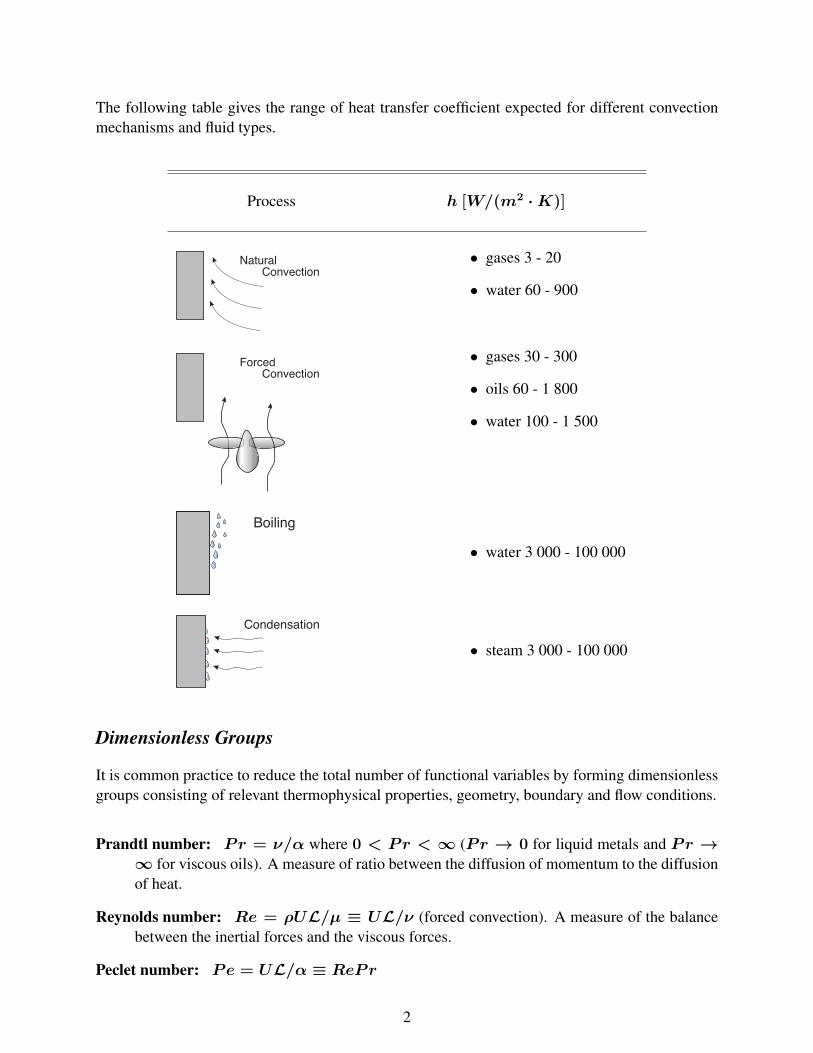
The following table gives the range of heat transfer coefficient expected for different convectionmechanisms and fluid types.

Process h [W/(m2 ·K)]

Natural

Convection

• gases 3 - 20

• water 60 - 900

Forced

Convection

• gases 30 - 300

• oils 60 - 1 800

• water 100 - 1 500

Boiling

• water 3 000 - 100 000

Condensation

• steam 3 000 - 100 000

Dimensionless Groups

It is common practice to reduce the total number of functional variables by forming dimensionlessgroups consisting of relevant thermophysical properties, geometry, boundary and flow conditions.

Prandtl number: Pr = ν/α where 0 < Pr < ∞ (Pr → 0 for liquid metals and Pr →∞ for viscous oils). A measure of ratio between the diffusion of momentum to the diffusionof heat.

Reynolds number: Re = ρUL/µ ≡ UL/ν (forced convection). A measure of the balancebetween the inertial forces and the viscous forces.

Peclet number: Pe = UL/α ≡ RePr

2

Grashof number: Gr = gβ(Tw − Tf)L3/ν2 (natural convection)

Rayleigh number: Ra = gβ(Tw − Tf)L3/(α · ν) ≡ GrPr

Nusselt number: Nu = hL/kf This can be considered as the dimensionless heat transfercoefficient.

Stanton number: St = h/(UρCp) ≡ Nu/(RePr)

Forced ConvectionThe simplest forced convection configuration to consider is the flow of mass and heat near a flatplate as shown below.

• as Reynolds number increases the flow has a tendency to become more chaotic resulting indisordered motion known as turbulent flow

– transition from laminar to turbulent is called the critical Reynolds number,Recr

Recr =U∞xcr

ν

– for flow over a flat plateRecr ≈ 500, 000

Boundary Layers

Velocity Boundary Layer

• the region of fluid flow over the plate where viscous effects dominate is called the velocityor hydrodynamic boundary layer

3

• the velocity of the fluid progressively increases away from the wall until we reach approxi-mately 0.99 U∞ which is denoted as the δ, the velocity boundary layer thickness.

Thermal Boundary Layer

• the thermal boundary layer is arbitrarily selected as the locus of points where

T − Tw

T∞ − Tw

= 0.99

Flow Over Plates

We will use empirical correlations based on experimental data where

Cf,x = C1 ·Re−m

Nux = C2 ·Rem · Prn =hx · xkf

4

1. Laminar Boundary Layer Flow, Isothermal (UWT)

The local values of the skin friction and the Nusselt number are given as

Cf,x =0.664

Re1/2x

Nux = 0.332Re1/2x Pr1/3 ⇒ local, laminar, UWT, Pr ≥ 0.6

An average value of the skin friction coefficient and the heat transfer coefficient for the full extentof the plate can be obtained by using the mean value theorem.

Cf =1.328

Re1/2L

NuL =hLL

kf= 0.664 Re

1/2L Pr1/3 ⇒ average, laminar, UWT, Pr ≥ 0.6

For low Prandtl numbers, i.e. liquid metals

Nux = 0.565Re1/2x Pr1/2 ⇒ local, laminar, UWT, Pr ≤ 0.6

2. Turbulent Boundary Layer Flow, Isothermal (UWT)

The local skin friction is given as

Cf,x =0.0592

Re0.2x

⇒ local, turbulent, UWT, Pr ≥ 0.6

Nux = 0.0296Re0.8x Pr1/3 ⇒local, turbulent, UWT,0.6 < Pr < 100, 500, 000 ≤ Rex ≤ 107

Cf,x =0.074

Re0.2x

⇒ average, turbulent, UWT, Pr ≥ 0.6

NuL = 0.037Re0.8L Pr1/3 ⇒average, turbulent, UWT,

0.6 < Pr < 100, 500, 000 ≤ Rex ≤ 107

5

3. Combined Laminar and Turbulent Boundary Layer Flow, Isothermal (UWT)

NuL =hLL

k= (0.037Re0.8L − 871) Pr1/3 ⇒

average, combined, UWT,0.6 < Pr < 60,500, 000 ≤ ReL ≤ 107

4. Laminar Boundary Layer Flow, Isoflux (UWF)

Nux = 0.453Re1/2x Pr1/3 ⇒ local, laminar, UWF, Pr ≥ 0.6

5. Turbulent Boundary Layer Flow, Isoflux (UWF)

Nux = 0.0308Re4/5x Pr1/3 ⇒ local, turbulent, UWF, Pr ≥ 0.6

Example 6-1: Hot engine oil with a bulk temperature of 60 ◦C flows over a horizontal, flatplate 5 m long with a wall temperature of 20 ◦C. If the fluid has a free stream velocity of2 m/s, determine the heat transfer rate from the oil to the plate if the plate is assumed to beof unit width.

6

Flow Over Cylinders and Spheres

1. Boundary Layer Flow Over Circular Cylinders, Isothermal (UWT)

The Churchill-Bernstein (1977) correlation for the average Nusselt number forlong (L/D > 100) cylinders is

NuD = 0.3 +0.62Re

1/2D Pr1/3

[1 + (0.4/Pr)2/3]1/4

1 +

(ReD

282, 000

)5/84/5

⇒ average, UWT,ReD < 107, 0 ≤ Pr ≤ ∞, ReD · Pr > 0.2

All fluid properties are evaluated at Tf = (Tw + T∞)/2.

2. Boundary Layer Flow Over Non-Circular Cylinders, Isothermal (UWT)

The empirical formulations of Zhukauskas and Jakob given in Table 12-3 are commonly used,where

NuD ≈hD

k= C RemD Pr

1/3 ⇒ see Table 12-3 for conditions

3. Boundary Layer Flow Over a Sphere, Isothermal (UWT)

For flow over an isothermal sphere of diameterD

NuD = 2 +[0.4Re

1/2D + 0.06Re

2/3D

]Pr0.4

(µ∞

µs

)1/4

⇒

average, UWT,0.7 ≤ Pr ≤ 380

3.5 < ReD < 80, 000

where the dynamic viscosity of the fluid in the bulk flow, µ∞ is based on the free stream tem-perature, T∞ and the dynamic viscosity of the fluid at the surface, µs, is based on the surfacetemperature, Ts. All other properties are based on T∞.

7

Example 6-2: An electric wire with a 1 mm diameter and a wall temperature of 325 Kis cooled by air in cross flow with a free stream temperature of 275 K. Determine the airvelocity required to maintain a steady heat loss per unit length of 70 W/m.

Internal Flow

The mean velocity and Reynolds number are given as

Um =1

Ac

∫Ac

u dA =m

ρmAc

ReD =UmD

ν

8

Hydrodynamic (Velocity) Boundary Layer

• the hydrodynamic boundary layer thickness can be approximated as

δ(x) ≈ 5x

(Umx

ν

)−1/2

=5x√Rex

• the hydrodynamic entry length can be approximated as

Lh ≈ 0.05ReDD (laminar flow)

Thermal Boundary Layer

• the thermal entry length can be approximated as

Lt ≈ 0.05ReDPrD = PrLh (laminar flow)

• for turbulent flow Lh ≈ Lt ≈ 10D

Wall Boundary Conditions

1. Uniform Wall Heat Flux: Since the wall flux qw is uniform, the local mean temperature de-noted as

Tm,x = Tm,i +qwA

mCp

will increase in a linear manner with respect to x.

The surface temperature can be determined from

Tw = Tm +qw

h

9

2. Isothermal Wall: The outlet temperature of the tube is

Tout = Tw − (Tw − Tin) exp[−hA/(mCp)]

Because of the exponential temperature decay within the tube, it is common to present themean temperature from inlet to outlet as a log mean temperature difference where

Q = hA∆Tln

∆Tln =Tout − Tin

ln

(Tw − Tout

Tw − Tin

) =Tout − Tin

ln(∆Tout/∆Tin)

10

1. Laminar Flow in Circular Tubes, Isothermal (UWT) and Isoflux (UWF)

For laminar flow whereReD ≤ 2300

NuD = 3.66 ⇒ fully developed, laminar, UWT, L > Lt & Lh

NuD = 4.36 ⇒ fully developed, laminar, UWF, L > Lt & Lh

NuD = 1.86

(ReDPrD

L

)1/3 (µb

µs

)0.14

⇒

developing laminar flow, UWT,Pr > 0.5

L < Lh or L < Lt

For non-circular tubes the hydraulic diameter, Dh = 4Ac/P can be used in conjunction withTable 10-4 to determine the Reynolds number and in turn the Nusselt number.

In all cases the fluid properties are evaluated at the mean fluid temperature given as

Tmean =1

2(Tm,in + Tm,out)

except for µs which is evaluated at the wall temperature, Ts.

2. Turbulent Flow in Circular Tubes, Isothermal (UWT) and Isoflux (UWF)

For turbulent flow whereReD ≥ 2300 the Dittus-Boelter equation (Eq. 13-68) can be used

NuD = 0.023Re0.8D Prn ⇒

turbulent flow, UWT or UWF,0.7 ≤ Pr ≤ 160

ReD > 2, 300

n = 0.4 heatingn = 0.3 cooling

For non-circular tubes, again we can use the hydraulic diameter,Dh = 4Ac/P to determine boththe Reynolds and the Nusselt numbers.

In all cases the fluid properties are evaluated at the mean fluid temperature given as

Tmean =1

2(Tm,in + Tm,out)

11

Natural Convection

What Drives Natural Convection?• fluid flow is driven by the effects of buoyancy

Natural Convection Over Surfaces

• note that unlike forced convection, the velocity at the edge of the boundary layer goes to zero

12

Natural Convection Heat Transfer Correlations

The general form of the Nusselt number for natural convection is as follows:

Nu = f(Gr, Pr) ≡ CGrmPrn where Ra = Gr · Pr

• C depends on geometry, orientation, type of flow, boundary conditions and choice of char-acteristic length.

• m depends on type of flow (laminar or turbulent)

• n depends on the type of fluid and type of flow

• Table 14-1 should be used to find Nusselt number for various combinations of geometry andboundary conditions

– for ideal gases β = 1/T∞, (1/K)

– all fluid properties are evaluated at the film temperature, Tf = (Tw + T∞)/2.

Natural Convection From Plate Fin Heat Sinks

The average Nusselt number for an isothermal plate fin heat sink with natural convection can bedetermined using

NuS =hS

kf=

[576

(RaSS/L)2+

2.873

(RaSS/L)0.5

]−0.5

13

A basic optimization of the fin spacing can be obtained as follows: For isothermal fins with t < S

Sopt = 2.714

(S3L

RaS

)1/4

= 2.714

(L

Ra1/4L

)

with

RaL =gβ(Tw − T∞)L3

ν2Pr

The corresponding value of the heat transfer coefficient is

h = 1.307kf/Sopt

All fluid properties are evaluated at the film temperature.

Example 6-3: Find the optimum fin spacing, Sopt and the rate of heat transfer, Q for thefollowing plate fin heat sink cooled by natural convection.

Given:

W = 120 mm H = 24 mmL = 18 mm t = 1 mmTw = 80 ◦C T∞ = 25 ◦CP∞ = 1 atm fluid = air

Find: Sopt and the corresponding heat transfer, Q

14