ControlsLabTM - Turbine Technologies Sample.pdf · Focus 4 - PID Tuning ... Unit 8 - Studio 5000...

ControlsLabTM

Programmable Automation Training

Curriculum Sample

Previous Next

2

Table of Contents

FLUIDMechatronixTM Fluid Process Automation System

Unit 1 - General Overview .......................................................................................... 10Chapter 1 - Overview of ControlsLabTM ....................................................................................11

Section 1: Description of System ........................................................................................... 13Focus 1: Electrical Schematics ....................................................................................... 13Focus 2: System Schematic ............................................................................................ 15Focus 3: System Parts .................................................................................................... 16Focus 4: System Capabilities .......................................................................................... 17

Section 2: Basic Blowing ........................................................................................................ 18Focus 1: Blower ............................................................................................................. 18

Section 4: PID Controls .......................................................................................................... 20Focus 1 - Height PID Control .......................................................................................... 20Focus 4 - PID Tuning ...................................................................................................... 22

Chapter 2 - Introduction to Automation .................................................................................... 23Section 1: The History of Automation ..................................................................................... 24

Focus 1: Manual Control ................................................................................................. 24Focus 2: Relays and Timers ............................................................................................ 25Focus 3: Programmable Relays ...................................................................................... 26

Section 2: Current Automation Technology ............................................................................ 27Focus 1: Programmable Automation Controller .............................................................. 27Focus 2: Communication Networks ................................................................................ 28

Chapter 3 - Introduction to PAC ................................................................................................ 29Section 1: Central Processing Unit ........................................................................................ 30

Focus 1: Microprocessor ................................................................................................. 30Focus 2: Advantages ....................................................................................................... 30Focus 3: Execute Instruction (Ladder Logic Basics) ....................................................... 31

Section 2: Scan-Cycle in PAC Operations ............................................................................. 32Focus 1: Parts of the Scan-Cycle .................................................................................... 32Focus 2: Input Scan ........................................................................................................ 32Focus 3: Execute Programs ............................................................................................ 33Focus 4: Output Scan ..................................................................................................... 33

Chapter 4 - Introduction to HMI ................................................................................................. 35Section 1 - History of the HMI ................................................................................................ 35

Focus 1 - What is an HMI? .............................................................................................. 35Focus 2: How does an HMI Work? ................................................................................. 37

Section 2: User Interface Software ........................................................................................ 38Focus 1: HMI Interface .................................................................................................... 38Focus 2: HMI Applications ............................................................................................... 39Focus 3: Software Advantages ....................................................................................... 40

Section 3: User Interface Controls ......................................................................................... 41Focus 1: Programmers ................................................................................................... 41Focus 2: Operators ......................................................................................................... 41

Chapter 5 - Introduction to VFD ................................................................................................ 42Section 1: VFD Basic Operation ............................................................................................ 43

Focus 1: Frequency ........................................................................................................ 43

Previous Next

3

Table of Contents


Focus 2: Voltage ............................................................................................................. 43Focus 3: Pulse Width Modulation (PWM) ....................................................................... 43

Section 2: Variable Frequency Drive Benefits ........................................................................ 45Focus 1: Speed Control .................................................................................................. 45Focus 2: Optimized Motor Starts ..................................................................................... 45Focus 3: Constant Torque ............................................................................................... 45

Chapter 6 - Introduction to Communications .......................................................................... 47Section 1: Serial Communication ........................................................................................... 48

Focus 1: The History of RS-232 ...................................................................................... 48Focus 2: RS-232 Uses in Automation ............................................................................. 49

Section 2: Ethernet Communication ...................................................................................... 50Focus 1: History of Ethernet ............................................................................................ 50Focus 2: Types of Ethernet Topology .............................................................................. 51Focus 3: How Ethernet is Useful ..................................................................................... 52

Chapter 7 - Introduction to Power ............................................................................................. 53Section 1: Basics of Power .................................................................................................... 54

Focus 1: What is Power? ................................................................................................ 54Focus 2: What is Voltage ................................................................................................ 55Focus 3: What is Current? .............................................................................................. 56Focus 4: What is Resistance? ......................................................................................... 57Focus 5: Ohm’s Law ........................................................................................................ 58Focus 4: Electrical Power ................................................................................................ 59

Section 2: Types of Power Supplies ...................................................................................... 60Focus 1: Switched Mode Supplies .................................................................................. 60Focus 2: Un-interruptible Power Supplies ....................................................................... 61

Section 3: Power Supply Requirements ................................................................................ 62Focus 1: Calculating Load ............................................................................................... 62Focus 2: Calculating Inrush ............................................................................................. 62Focus 3: Choosing a Power Supply ................................................................................ 63

Unit 2 - Centrifugal Blowing ...................................................................................... 64Section 1: Define Centrifugal Blowing .................................................................................... 65

Chapter 1 - Introduction to Centrifugal Blowing ...................................................................... 65Focus 1: Let’s Fling Stones! ........................................................................................... 67

Section 2: Specific Gravity of a Fluid ..................................................................................... 71Section 3: Introduction to Suction .......................................................................................... 73

Focus 1: Suction Lift ........................................................................................................ 73Focus 2 :Capacity and Suction Lift .................................................................................. 77

Section 4: Net Positive Suction Head (NPSH) & Cavitation .................................................. 79Focus 1: Net Positive Suction Head Available (NPSHa) ................................................. 80Focus 2: Net Positive Suction Head Required (NPSHr) ................................................. 82

Chapter 2 - Introduction to Process Control ............................................................................ 85Section 1: Define Process Control ......................................................................................... 85

Focus 1: Watering the Lawn ............................................................................................ 85Section 2: Electric Motor Operation; a Blower’s Driving Force .............................................. 87

Previous Next

4

Table of Contents


Focus 1: Components of an Electric Motor ..................................................................... 87Focus 2: What is Electric Frequency ............................................................................... 88Focus 3: RPM as a Function of Frequency in a Single Phase Motor .............................. 90Focus 4: Three Phase Motors ......................................................................................... 91

Section 3: Variable Frequency Drives .................................................................................... 93Focus 1: Rectifier ............................................................................................................ 94Focus 2: Direct Current Bus (DC Bus) ............................................................................ 95Focus 3: Inverter ............................................................................................................. 95Focus 4: Output of the Inverter ....................................................................................... 96Focus 5: Effective Voltage ............................................................................................... 97

Section 4: Variable Speed Applications in Blowing .............................................................. 100Focus 1: Constant Pressure .......................................................................................... 100Focus 2: Constant Flow ................................................................................................ 102Focus 3: Variable Flow .................................................................................................. 103Focus 4: Soft Start ........................................................................................................ 103

Section 5: Process Control Logic ......................................................................................... 105Focus 1: Open Loop Control: A Return to Watering the Lawn ...................................... 105Focus 2: Closed Loop Control: The Heating System .................................................... 105Focus 3: Getting a Better Feel for Controller Logic (Hand-Controlling the Process). ... 106

Section 6: The PID Controller .............................................................................................. 108Focus 1: PID Control Overview .................................................................................... 108Focus 2: Proportional Control (The P in PID) ................................................................ 111Focus 3: Integral Control (The I in PID) ........................................................................114Focus 4: Derivative Control (The D in PID) ....................................................................116Focus 5: Putting It All Together: PID Control ..................................................................117

Section 7: Tuning Methodologies-An introduction to Gain .................................................. 120Focus 1: Introduction to Gain ........................................................................................ 120Focus 2: Manual Tuning-Trial and Error ........................................................................ 120Focus 3: The Ziegler-Nichols Method ........................................................................... 121Focus 4: PID Tuning Software ...................................................................................... 121

Unit 3 - Ethernet Communication ............................................................................ 122Chapter 1 - Introduction to Ethernet ....................................................................................... 123

Section 1: What is Ethernet? ............................................................................................... 124Focus 1: Types of Ethernet ........................................................................................... 124Focus 2: Types of LAN Technology ............................................................................... 125Focus 3: IP (Internet Protocol) ...................................................................................... 126Focus 4: TCP (Transmission Control Protocol) ............................................................. 127Focus 5: UDP (User Datagram Protocol) ...................................................................... 128Focus 6: IP Addressing ................................................................................................. 129

Section 2: Types of Switched Ethernet ................................................................................ 130Focus 1: Basic Switches ............................................................................................... 130Focus 2: Intelligent Switches ......................................................................................... 131Focus 3: Managed Switches ......................................................................................... 132

Chapter 2 - Network Setup ....................................................................................................... 134

Previous Next

5

Table of Contents


Section 1 - IP Address Classification ................................................................................... 134Focus 1: Binary Code .................................................................................................... 134Focus 2: Addressing ...................................................................................................... 135Focus 3: Classes ........................................................................................................... 136

Section 2: Subnets ............................................................................................................... 139Focus 1: What are Subnets? ......................................................................................... 139Focus 2: Subnet Benefits .............................................................................................. 139

Section 3: IP Routing ........................................................................................................... 141Focus 1: What is IP Routing? ........................................................................................ 141Focus 2: Routers ........................................................................................................... 141

Chapter 3 - Communication Setup .......................................................................................... 143Section 1: PAC Ethernet Setup ........................................................................................... 144

Focus 1: IP Address Setup with USB ............................................................................ 144Section 1: PAC Ethernet Setup ........................................................................................... 145Section 1: PAC Ethernet Setup ........................................................................................... 146Section 1: PAC Ethernet Setup ........................................................................................... 147

Focus 2: Other IP Address Setup Methods .................................................................. 147Section 2: HMI Ethernet Setup ........................................................................................... 148Section 3: VFD Ethernet Setup ............................................................................................ 150

Chapter 4 - Ethernet with Wireless Technology ................................................................... 151Section 1 - Introduction to WLAN ......................................................................................... 151

Focus 1 - What is WLAN? ............................................................................................. 151Focus 2 - Access Points ................................................................................................ 152Focus 3 - Security ......................................................................................................... 153Focus 4 - Interference ................................................................................................... 154

Unit 4 - Programmable Automation Controller ...................................................... 156Chapter 1 - Introduction to CompactLogix 5370 L1 Controller ............................................ 157

Section 1: 1769-L16ER Controller ....................................................................................... 158Focus 1: Memory .......................................................................................................... 158Focus 2: Embedded Inputs / Outputs ............................................................................ 159Focus 3: 1734 Series Expansion Cards ........................................................................ 163

Section 2: Communication .................................................................................................. 165Section 2: Communication .................................................................................................. 166

Chapter 2 - Embedded Input / Output ..................................................................................... 167Section 1: Inputs .................................................................................................................. 168

Focus 1: Analog Laser .................................................................................................. 168Section 2: Outputs ............................................................................................................... 170

Focus 1: Louvers ........................................................................................................... 170Section 3: Sports Drink Scenario ......................................................................................... 171

Focus 1 - Start the Process ........................................................................................... 171Focus 2 - Fluid Process ................................................................................................ 172Focus 3 - Back to the Process Tank .............................................................................. 173

Chapter 3 - I / O Expansion Modules ...................................................................................... 176Section 1: 1734 Module Installation ..................................................................................... 177

Previous Next

6

Table of Contents


Focus 1 - 1734 Point I/O System .................................................................................. 177Focus 2 - 1734 Point I/O Features ................................................................................ 178Focus 3 - 1734 Module Installation ............................................................................... 179Focus 4 - Wiring the Modules ....................................................................................... 182

Section 5: Pharmaceutical Scenario .................................................................................... 184Focus 1 - Process Plant ................................................................................................ 184Focus 2 - Buffering and Bottling a Batch of Eyedrops................................................... 186Focus 3 - Buffering and Bottling a Batch of Contact Lens Solution............................... 189

Chapter 4 - Tag Database ......................................................................................................... 194Section 1: Project Structure ................................................................................................. 195

Focus 1 - Project ........................................................................................................... 195Focus 2 - Task ............................................................................................................... 196Focus 3 - Programs ....................................................................................................... 197Focus 4 - Routines ........................................................................................................ 198Focus 1 - Tag Memory ................................................................................................... 199Focus 2 - Tag Naming Rules ......................................................................................... 200Focus 3 - I/O Tag Format .............................................................................................. 201Focus 4 - Tag Locations ................................................................................................ 202

Section 2: Tag Basics ........................................................................................................... 203Focus 5 - ControlsLabTM Tag Library ............................................................................ 203

Section 3: Types of Tags ...................................................................................................... 206Focus 1: BOOL Tags ..................................................................................................... 206Focus 2: DINT Tags ....................................................................................................... 207Focus 3: REAL Tags ...................................................................................................... 208Focus 4: STRINGS ....................................................................................................... 209

Unit 5 - Human Machine Interface ............................................................................211Chapter 1 - Introduction to ControlsLab HMI ......................................................................... 212

Section 1: ControlsLab HMI Computer ................................................................................ 213Focus 1: Windows 8.1 Pro Operating System and Features ........................................ 213Focus 2: 8 GB RAM ...................................................................................................... 216Focus 3: 128 GB Solid State Drive ............................................................................... 217Focus 4: 1.8 GHz Quad-Core Processor N9230 ........................................................... 218

Section 2: Communication I/O ............................................................................................ 219Focus 1: Dual LAN (Ethernet) Inputs ............................................................................ 219Focus 2: Dual Video Outputs ........................................................................................ 220Focus 3: Dual USB 3.0 I/O ............................................................................................ 221

Chapter 2 - HMI Software ......................................................................................................... 222Section 1: Introduction to Studio 5000 Logix Designer ........................................................ 223

Focus 1: Creating a New Project .................................................................................. 223Focus 2: Ladder Logic ................................................................................................... 227Focus 3: Adding Expansion Modules ............................................................................ 232Focus 4: Function Block Diagram ................................................................................. 237Focus 5: Structured Text ............................................................................................... 249Focus 6: I/O Tag Data ................................................................................................... 260

Previous Next

7

Table of Contents


Section 2: Introduction to FactoryTalk View ME ................................................................... 264Focus 1: Creating a New Run-Time .............................................................................. 264Focus 2: Communication Setup .................................................................................... 276Focus 3: Global Objects ................................................................................................ 280Focus 4: Displays .......................................................................................................... 292Focus 5: Faceplates ...................................................................................................... 309Focus 6: Tags ................................................................................................................ 319Focus 7: Alarms ............................................................................................................ 327Focus 8: Buttons ........................................................................................................... 338

Chapter 4 - VNC Control ........................................................................................................... 346Section 1: VNC Server ......................................................................................................... 347

Focus 1: Introduction to VNC ........................................................................................ 347Focus 2: HMI VNC Server ............................................................................................. 348

Section 2: VNC Client .......................................................................................................... 353Focus 1: Connecting to a VNC Server with Client Software ......................................... 353

Unit 6 - Variable Frequency Drive ........................................................................... 356Chapter 1 - Introduction to PowerFlex 525 ............................................................................. 357

Section 1: Drive Setup ......................................................................................................... 358Focus 1: Drive Wiring .................................................................................................... 358Focus 2: I/O Features ................................................................................................... 361

Section 2: Drive Parameters ............................................................................................... 362Focus 1: Parameter Basics ........................................................................................... 362Focus 2: Ethernet Parameters ...................................................................................... 366

Chapter 2 - VFD Software Control ........................................................................................... 369Section 1: Basic Control ....................................................................................................... 370

Focus 1: VFD Software Configuration ........................................................................... 370Focus 2: Studio 5000 Control Setup ............................................................................. 382Focus 3: FactoryTalk View ME VFD Control ................................................................. 397

Section 2: PIDE Control ....................................................................................................... 410Focus 1: Studio 5000 PIDE Setup ................................................................................ 410Focus 2: FactoryTalk View ME PIDE Setup .................................................................. 428

Unit 8 - Studio 5000 Logix Designer ....................................................................... 438Chapter 1 - Introduction Studio 5000 Logix Designer ........................................................... 439

Section 1: Creating a Project ............................................................................................... 439Section 2: Connecting Your Computer to the Controller ...................................................... 439Section 3: Downloading Project from the Computer to the Controller ................................. 439Section 4: Configuring I/O .................................................................................................... 439Section 5: Testing Your Logic Program ................................................................................ 439Section 6: Adding Logic and Tags Online ............................................................................ 439Section 7: Creating and Running a Trend ............................................................................ 439Section 8: (Optional) Creating and Using User Defined Types (UDT) ................................. 439Section 9: (Optional) Using Studio 5000 Help ..................................................................... 439

Chapter 2 - I/O and Tag Data .................................................................................................... 440Section 1: Communicate with I/O Modules .......................................................................... 440

Previous Next

8

Table of Contents


Section 2: Organize Tags ..................................................................................................... 440Section 3: Force I/O ............................................................................................................. 440Section 4: Data Access Control ........................................................................................... 440

Chapter 3 - Ladder Logic Programming ................................................................................. 441Section 1: Introduction ......................................................................................................... 441Section 2: Write Ladder Logic .............................................................................................. 441Section 3: Enter Ladder Logic .............................................................................................. 441Section 4: Assign Instruction Operands ............................................................................... 441Section 5: Enter A Rung Comment ...................................................................................... 441Section 6: Verify the Routine ................................................................................................ 441

Chapter 4 - Structured Text Programming ............................................................................. 442Section 1: Introduction ......................................................................................................... 442Section 2: Assignments ........................................................................................................ 442Section 3: Expressions ........................................................................................................ 442Section 4: Instructions .......................................................................................................... 442Section 5: Constructs ........................................................................................................... 442Section 6: If . . . Then ........................................................................................................... 442Section 7: Case . . . Of ......................................................................................................... 442Section 8: For . . . Do ........................................................................................................... 442Section 9: While . . . Do ....................................................................................................... 442Section 10: Repeat . . . Until ................................................................................................ 442

Chapter 5 - Function Block Diagram Programming .............................................................. 443Section 1: Introduction ......................................................................................................... 443Section 2: Choose the function block .................................................................................. 443Section 3: Choose a tag name for an element .................................................................... 443Section 4: Define the order of execution .............................................................................. 443Section 5: Identify any connectors ...................................................................................... 443Section 6: Define program/operator control ......................................................................... 443Section 7: Add a sheet ......................................................................................................... 443Section 8: Add a function block element .............................................................................. 443Section 9: Create a text box ................................................................................................. 443Section 10: Connect elements ............................................................................................. 443Section 11: Assign a tag ....................................................................................................... 443Section 12: Assign an immediate value (constant) .............................................................. 443Section 13: Connect blocks with an OCON and ICON ........................................................ 443Section 14: Verify the routine .............................................................................................. 443

Chapter 6 - Plant PAX ............................................................................................................... 444Section 1 - PlantPAX Library of Process Objects ................................................................ 444

Focus 1: Overview ........................................................................................................ 444Focus 2: How to Install the Library ................................................................................ 444Focus 3: Common Configuration Considerations ......................................................... 444Focus 4: Use the Library ............................................................................................... 444

Section 2: P_RunTime ......................................................................................................... 445Section 3: P_VSD ................................................................................................................ 446Section 4: P_Perm ............................................................................................................... 447

Previous Next

9

Table of Contents


Section 5: P_Intlk ................................................................................................................. 448Section 6: P_Alarm .............................................................................................................. 449Section 7: P_AIn .................................................................................................................. 450Section 8: P_Mode ............................................................................................................... 451Section 9: P_PIDE ............................................................................................................... 452

Unit 9 - FactoryTalk View ME ................................................................................... 453Chapter 1 - FactoryTalk View ME User’s Guide ..................................................................... 454

Section 1: Getting Started .................................................................................................... 454Section 2: Explore FactoryTalk View Studio ........................................................................ 454Section 3: Plan applications ................................................................................................. 454Section 4: Work with applications ........................................................................................ 454Section 5: Set up communications ....................................................................................... 454Section 6: Work with tags .................................................................................................... 454Section 7: Use HMI tags ...................................................................................................... 454Section 8: Set up global connections ................................................................................... 454Section 9: Set up alarms ...................................................................................................... 454Section 10: Set up FactoryTalk Diagnostics ......................................................................... 454Section 11: Set up security .................................................................................................. 454Section 12: Set up language switching ................................................................................ 454Section 13: Set up display navigation .................................................................................. 454Section 14: Create run-time applications ............................................................................. 454Section 15: Run applications on a personal computer ......................................................... 454Section 16: Transfer applications to a PanelView Plus terminal .......................................... 454Section 17: Use your application ......................................................................................... 455Section 18: Work with components ...................................................................................... 455Section 19: Use graphic displays ......................................................................................... 455Section 20: Use graphic objects .......................................................................................... 455Section 21: Set up graphic objects ...................................................................................... 455Section 22: Animate graphic objects .................................................................................... 455Section 23: Use expressions ............................................................................................... 455Section 24: Use embedded variables .................................................................................. 455Section 25: Use parameters and global objects .................................................................. 455Section 26: Set up data logging ........................................................................................... 455Section 27: Use information messages ............................................................................... 455Section 28: Set up trends ..................................................................................................... 455Section 29: Set up RecipePlus ............................................................................................ 455Section 30: Use macros ....................................................................................................... 455

Previous Next

10

HMI

PAC

Ethernet

DC Supply

VFD

Unit 1 - General Overview

Previous Next

24UNIT 1 - GENERAL OVERVIEWCHAPTER 2 - Introduction to Automation

Chapter 2 - Introduction to Automation

Introduction

Industrial Automation is the automatic operation or control of equipment, processes, or systems using techniques and equipment to achieve this condition.

Section 1 – History of Automation• Manual Control• Relays and Timers• Programmable Relays

Section 2 – Current Automation Technology• Process Logic Controller (PAC)• Communication Network

Previous Next


Section 1: The History of Automation

Focus 1: Manual Control

Before the advent of modern control systems, operators had to “operate” processes by hand. If a valve needed to be opened or closed it was done by hand. If a blower needed to be started, a human operator had to start it. Human errors, and consequently its effect on quality of final product, made early automation practices difficult. The production, safety, energy consumption and usage of raw material are all subject to the correctness and accuracy of human action.

Automation is the use of automatic machinery and systems, particularly those manufacturing or data processing systems which require little or no human intervention in their normal operation. During the 19th century a number of machines such as looms and lathes became increasingly self-regulating. At the same time transfer-machines were developed, whereby a series of machine-tools, each doing one operation automatically, became linked in a continuous production line by pneumatic or hydraulic devices transferring components from one operation to the next. Manual control led the industrial automation environment until the 1950s, when relay control gave the operator the ability to control more than one thing at a time.

Primitive Automation Based on Manual Controls

Previous Next


Focus 2: Relays and Timers

In the early part of the 20th century, industrial relays and timers were invented and applied to systems in a crude measure to provide some relief to the vast number of plant operators required. This was the start of “automating” processes. These processes became automatically controlled, and a number of basic industries such as oil-refining, chemicals, and food-processing were increasingly automated. The development of computers after World War II enabled more sophisticated automation to be used in manufacturing industries, for example iron and steel. A major benefit to this early automation process was improved operator safety.


Relay and Timer Control Board

Previous Next


Focus 3: Programmable Relays

The next step in automation advancement was the programmable relay, which was able to actually hold a few lines of code that would allow it to react to inputs and control outputs. In more recent years, small products called PLRs (programmable logic relays), and also by similar names, have become more common and accepted. These are much like PACs, and are used in light industry where only a few points of I/O (i.e. a few signals coming in from the real world and a few going out) are needed, and low cost is desired. These small devices are typically made in a common physical size and shape by several manufacturers, and branded by the makers of larger PACs to fill out their low end product range.

Popular names include PICO Controller, NANO PAC, and other names implying very small controllers. Most of these have 8 to 12 discrete inputs, 4 to 8 discrete outputs, and up to 2 analog inputs. Size is usually about 4” wide, 3” high, and 3” deep. Most such devices include a tiny postage-stamp-sized LCD screen for viewing simplified ladder logic (only a very small portion of the program being visible at a given time) and status of I/O points, and typically these screens are accompanied by a 4-way rocker push-button plus four more separate push-buttons, similar to the key buttons on a VCR remote control, and used to navigate and edit the logic. Most have a small plug for connecting via RS-232 or RS-485 to a personal computer so that programmers can use simple Windows applications for programming instead of being forced to use the tiny LCD and push-button set for this purpose. Unlike regular PACs that are usually modular and greatly expandable, the PLRs are usually not modular or expandable, but their price can be two orders of magnitude less than a PAC, and they still offer robust design and deterministic execution of the logics. PLRs are still in use today as a lower-level automation device.


Programmable Logic Relay

Previous Next


Section 2: Current Automation Technology

Focus 1: Programmable Automation Controller

Programmable Automation Controllers, also known as PACs, are the latest advanced technology used to take industrial automation to a new level. It is able to take in a high number of process data inputs and schedule outputs that enable an automated system to work. PACs have continued to improve over the last few years. They have an increasing number of inputs and greater processing power as technology advances. PACs have advanced beyond the capabilities of PLCs (programmable logic controllers).

1. What was the biggest problem with manual control?

2. What was the main benefit to relay control?

3. What does a PLR typically show on the LCD display?

Section 1, Focus 1-3

Programmable Logic Controller

Previous Next


Focus 2: Communication Networks

Industrial automation uses a variety of communication networks to allow automation components to “talk” to each other. The different forms of communication networks include:

Ethernet/IP: Ethernet Industrial Protocol is built on standard TCP/IP (IEEE 802.3) and communications use existing network infrastructure. Ethernet physical layer technology is used along TCP and UDP ports (44818 and 2222). Its main advantage comes from the inerrant progress of physical Ethernet, from 10 Mbits/s to 10/100 Mbits/s to 1 Gbits/s and more. Ethernet/IP also ensures Internet and enterprise connectivity for remote control.

ControlNet: Built on its own physical and data link layer, ControlNet uses a single media link with (inexpensive) RG-6 coaxial cables and bus. It features a 5 Mbits/s speed, upload/download of data, P2P communication, and up to 99 nodes.

DeviceNet: Uses Controller Area Network (CAN-bus) as a backbone for physical and data link layer. CAN-bus consists of a host processor, a controller, and a transceiver linked by 2 twisted pair cables. Bit rates go from 1 Mbit/s at 40 m to 20 Kbit/s at 1200 m. DeviceNet uses the master/slave mode; it can have up to 64 nodes and the physical network can provide power to the devices (with limited consumption).

Modbus: Based on the master/slave mode and having up to 247 nodes, Modbus has many protocol versions depending on the physical layer being used. Every version uses the same base communication going from start, address, function, date, error check, and end.

Profibus: Using master-slave, slave-slave, and master-master communication on a bit serial field. The physical layer can be a twisted pair cable delivering power to the device and providing 9.6 kbit/s to 12 Mbit/s (maximum 1200 m) or an optical fiber cable.

EtherCAT: Ethernet for Control Automation Technology is based on the Ethernet technology and uses twisted pair cables or coaxial cables with BNC adapters on a short distance (1000 m max.) and an optical fiber cable over long distances. Transfer rates are based on the Ethernet technology being used and EtherCAT can control up to 65535 nodes.

CC-Link: An open protocol for industrial networks that include protocols for the information network, the controller network, and the device field network. The version of CC-link depends on the physical layer being used. The protocol can normally have up to 64 nodes and have speed going from 10 Mbps at 100 meters to 156 Kbps at 1200 meters.

Section 2: Current Automation Technology

Previous Next

30UNIT 1 - GENERAL OVERVIEWCHAPTER 3 - Introduction to PLC

Chapter 3 - Introduction to PAC

Section 1 – Central Processing Unit• Microprocessor• Advantages• Execute Instruction

Section 2 – Scan-Cycle in the PAC• Parts of the Scan-Cycle• Input Scan• Execute Programs• Output Scan

Introduction

A Programmable Automation Controller (PAC) is a very scalable controller that can handle 100’s of inputs, control 100’s of outputs and takes automation to its highest level. It is designed and built to be very robust to endure environments with noise, field interference and variable power. It is simple by design to avoid crashes and glitches; this is very important when controlling industrial equipment. PACs are designed to control equipment in harsh environments and not fail. If they do fail, they are designed to fail in the safest manner possible.

The PAC was originally invented to support the automotive manufacturing industry. It replaced the large relay networks, which were complicated to troubleshoot and unreliable.

Before the PAC, control, sequencing, and safety interlock logic for manufacturing automobiles relied on hundreds or, in some instances, thousands of relays, cam timers, and drum sequencers and dedicated closed-loop controllers. The process for updating such facilities for the yearly model change-over was very time consuming and expensive, as electricians needed to individually and manually rewire each and every relay.

In 1968 GM Hydramatic issued a request for proposal for an electronic replacement for hard-wired relay systems. The winning proposal came from Bedford Associates of Bedford, Massachusetts. The first PAC, designated the 084 because it was Bedford Associates eighty-fourth project, was the result. Bedford Associates started a new company dedicated to developing, manufacturing, selling, and servicing this new product: MODICON, which stood for MOdular DIgital CONtroller. One of the people who worked on that project was Dick Morley, the “father” of the PAC.

In other industries, PACs replaced relay systems used in manufacturing applications. This eliminated the high cost of maintaining these inflexible systems. In 1970, with the innovation of the microprocessor, the machine that was originally used as a relay replacement device only, evolved into the advanced PAC of today.

Previous Next


Section 1: Central Processing Unit

Focus 1: Microprocessor

A Programmable Automation Controller (PAC) is a very scalable controller that can handle 100’s of inputs, control 100’s of outputs and takes automation to its highest level. It is designed and built to be very robust to endure environments with noise, field interference and variable power. It is simple by design to avoid crashes and glitches; this is very important when controlling industrial equipment. PACs are designed to control equipment in harsh environments and not fail. If they do fail, they are designed to fail in the safest manner possible. The function of the CPU is to store and run the PAC software programs. It also interfaces with the Co-Processor Modules, the I/O Modules, the peripheral device, and runs diagnostics. It is essentially the “brains” of the PAC.

Focus 2: Advantages

Relay systems were cheap and reliable, but they were quickly replaced by PACs because of their processing advantages:

Flexibility: One single PAC can easily monitor and run many machines.

Ease of Troubleshooting: Back before PACs, wired relay-type panels required time for rewiring of panels and devices. With PAC control any change in circuit design or sequence is as simple as retyping the logic. Correcting errors in PAC is both fast and cost effective.

Space Efficient: Fewer components are required in a microprocessor system than in a conventional hardware system. The processor performs the functions of timers, counters, sequencers, and control relays, so these hardware devices are not required. The only field devices that are required are those that directly interface with the system such as switches and motor starters.

Low Cost: Prices of microprocessors vary from few hundreds to few thousands. This is minimal compared to the prices of the contact, coils, and timers that companies pay to match the same things. Using PACs also saves on installation cost and shipping.

Visual observation: When running a microprocessor users have an advantage of receiving feedback from the controller and that can be easily monitored with a screen or display.

Previous Next


Focus 3: Execute Instruction (Ladder Logic Basics)

Ladder logic is a programming language that represents a program by a graphical diagram based on the circuit diagrams of relay-based logic hardware. It is primarily used to develop software PACs used in industrial control applications. The name is based on the observation that programs in this language resemble ladders, with two vertical rails and a series of horizontal rungs between them. Ladder logic is widely used to program PACs, where sequential control of a process or manufacturing operation is required. Ladder logic is useful for simple but critical control systems, or for reworking old hardwired relay circuits. As PACs became more sophisticated, it has also been used in very complex automation systems. Often the ladder logic program is used in conjunction with a HMI program operating on a computer workstation.

Manufacturers of programmable automation controllers generally also provide associated ladder logic programming systems. Typically, the ladder logic languages from two manufacturers will not be completely compatible; ladder logic is better thought of as a set of closely related programming languages rather than one language (which is covered in Unit 8). Even different models of PACs within the same family may have different ladder notation such that programs cannot be seamlessly interchanged between models.

Section 1: Central Processing Unit

1. What is the brains of the PAC?

2. Name the 5 advantages of the microprocessor?

3. What logic was ladder logic based upon?

Section 1: Focus 1-3

Ladder Logic Rung Diagram

Previous Next


Section 2: Scan-Cycle in PAC Operations

Focus 2: Input Scan

A simple way of looking at this is the PAC takes a snapshot of the inputs and solves the logic. The PAC looks at each input card to determine if it is ON or OFF and saves this information in a data table for use in the next step. This makes the process faster and avoids cases where an input changes from the start to the end of the program.

Introduction: Basic Operation of a PAC

Focus 1: Parts of the Scan-Cycle

PAC operations can be broken down into a few parts. The processor makes decisions based on programmed instructions, “ladder logic,” written by the user. The PAC examines the logic and communicates with the various field devices it monitors and controls. It can read the actual conditions of the field devices and execute program instructions based on those values. If the program determines that changes are required, it can outputs to update the devices. Here is an example of how a PAC program runs a basic switch:

1. Input switch is pressed2. Input module places a “1” in the input data table3. The ladder logic program sees the “1” and caused a “1” to be put into the output data table4. The output data table causes the output module to energize associated point5. The output device energizes

PACs operate by continually scanning programs and repeat this process about ten times per second. When a PAC starts, it runs checks on the hardware and software for faults, also called a self-test. If there are no problems, then the PAC will start the scan cycle. The scan cycle consists of three steps: input scan, executing program(s), and output scan.

CPU Checks

I/O Module Checks

Scan Inputs

Execute Program

Update Checks

Pre-Scan

Previous Next


Focus 3: Execute Programs

The PAC executes a program one instruction at a time using only the memory copy of the inputs the ladder logic program. For example, the program has the first input as ON. Since the PAC knows which inputs are ON/OFF from the previous step, it will be able to decide whether the first output should be turned ON.

Ladder logic programs are modeled after relay logic. In relay logic, each element in the ladder will switch as quickly as possible. Program elements can only be examined one at a time in a fixed sequence. The ladder logic scan begins at the top rung. At the end of the rung, it interprets the top output first, and then the output branched below it. On the second rung, it solves branches, before moving along the ladder logic rung.

The language itself is a set of connections between logical checkers (contacts) and actuators (coils). If a path traced between the left side of the rung and the output, through asserted (true or closed) contacts, the rung is true and the output coil storage bit is asserted 1. If no path is traced, then the output is false (0) and the coil by analogy to electromechanical relays is considered de-energized. Ladder logic has contacts that make or break circuits to control coils. Each coil or contact corresponds to the status of a single bit in the PACs memory. Unlike electromechanical relays, a ladder program can refer any number of times to the status of a single bit, equivalent to a relay with an indefinitely large number of contacts.

Focus 4: Output Scan

When the ladder scan completes, the outputs are updated using the temporary values in memory. The PAC updates the status of the outputs based on which inputs were ON during the first step and the results of executing a program during the second step. The PAC now restarts the process by starting a self-check for faults.


Scan Inputs

Execute Program

Update Outputs

Previous Next


1. Name the three parts of the scan-cycle.

2. What is the purpose of the input scan?

3. Describe how a PAC executes logic.

4. What happens after the scan-cycle is complete?

Section 2: Focus 1-4


Previous Next

65

Unit 2 - Centrifugal Blowers

Previous Next

86UNIT 2 - CENTRIFUGAL PUMPINGCHAPTER 2 - Introduction to Process Control

Process control is the ability to manipulate or control an operation on a consistent basis to produce reliable desired outcomes. In blowing, this means controlling a blower to produce desired flow and/or pressure results in the system in which it is operating. This usually means the system environment offers “feedback” information to the blower so that it can automatically adjust how it runs in order to properly meet the situation requirements.

Process control is extensively used in industry and enables mass production of continuous processes such as oil refining, paper manufacturing, chemical formulation, electric power production and many other industries. Process control enables automation which allows a small staff of operating personnel to operate a complex process from a central control room.

Centrifugal blowers are used extensively in industry to direct the flow of fluids for countless processes. Controlling and integrating this flow is now typically handled by a programmable Variable Frequency Drive (VFD). VFDs can be programmed to control the speed of the electric motor driving the blower, essentially making it a variable speed unit to meet very particular blowing needs. It also can be part of a larger control scheme where many blowers are controlled and scheduled automatically to produce a desired final result. Feedback Loops are a part of process control that provide information to the VFD regarding adjustments that need to be made to the blower speed to enable it to maintain the desired end result.

Let’s start with a simple operation that illustrates developing process control

You move to a new house with a dry-looking lawn. You decide to water it by connecting a hose to your water supply, turning it on and hand spraying it by walking around the property. The next day you do it again. Since you have better things to do than spend your time walking around the lawn, you add an oscillating lawn sprinkler to the end of the hose and set an alarm for yourself to move it every half hour. Notice that you are establishing a “process” and “controlling” it to accomplishing the “result” of watering the lawn. Each day the lawn needs water, so you repeat this process. Finally, you tire of this “monitor and move” operation, so you have a sprinkler system installed which covers your whole lawn. The system has a control on it so you can set the time of day you want the sprinkler to come on and how long it should run. Your process is now perfectly automated to come on at a pre-set time and water the lawn for a fixed amount of time.

Section 1: Define Process Control

Figure 1.1: Watering the Lawn

Approximate Lesson Duration: 10 min.

Focus 1: Watering the Lawn

Upon completion of this book, the student will have a good understanding of the important issues of process control as it relates to centrifugal blowing, including; Variable Frequency Drive Operation, Open and Closed Loop Systems, Feedback Loop, Proportional, Integral and Derivative Algorithm and Gain. This knowledge will serve as the foundation for learning to effectively use centrifugal blowing in liquid process scenarios.

Chapter 2 - Introduction to Process Control


Previous Next


Section 1, Focus 1

You install a yard light that is activated by a manual switch. You decide to put it on an automatic timer so that is comes on and goes off at prescribed times. As the seasons change, it gets darker earlier and stays darker later resulting in times where the field is too dark to use. What sort of “feedback” from your environment would help this situation?

You are very pleased with yourself until later that week you notice your lawn sprinkler is on during a driving rainstorm. Ouch! The process wasn’t getting any “feedback” that it wasn’t needed, so it came on as scheduled. That’s when you decide to install a moisture sensor on your lawn that is connected to your sprinkler. If the moisture level of the lawn was reading high enough, it signaled the sprinkler not to launch during the programmed launch time. It also sensed when the moisture level was high enough during sprinkling to shut the sprinkler system off early. Now you have a “process” that is “controlled” automatically with proper “feedback”, which accomplishes the mission of watering the lawn in a reliable, convenient, repeatable and cost effective manner.

Blowers can be operated in a similar fashion; from basic manual control at constant speed, all the way to fully automatic control using a variable speed controller tied to some sort of system “feedback loop”. A blower driven by an electric motor can be controlled by a variable frequency drive. Why is this important? It offers greatly improved fluid processing control while using the electricity to drive it much more efficiently. These two factors improve the end use result while saving substantially on energy. Let’s find out how this happens. The following lessons will introduce topics that build toward better understanding of blowing process control.


Previous Next


In this lesson, the student will learn important characteristics of electric motors which drive blowers. Topics will include electric motor components, electrical frequency, single and three phase motors. Understanding these basic elements helps a student to understand how an electric motor is controlled in a process control environment.

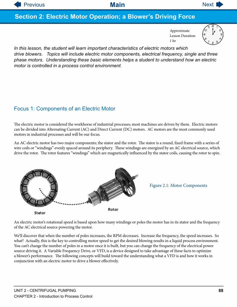
Focus 1: Components of an Electric Motor

The electric motor is considered the workhorse of industrial processes; most machines are driven by them. Electric motors can be divided into Alternating Current (AC) and Direct Current (DC) motors. AC motors are the most commonly used motors in industrial processes and will be our focus.

An AC electric motor has two major components; the stator and the rotor. The stator is a round, fixed frame with a series of wire coils or “windings” evenly spaced around its periphery. These windings are energized by an AC electrical source, which drive the rotor. The rotor features “windings” which are magnetically influenced by the stator coils, causing the rotor to spin.

Figure 2.1: Motor Components

An electric motor’s rotational speed is based upon how many windings or poles the motor has in its stator and the frequency of the AC electrical source powering the motor.

We’ll discover that when the number of poles increases, the RPM decreases. Increase the frequency, the speed increases. So what? Actually, this is the key to controlling motor speed to get the desired blowing results in a liquid process environment. You can’t change the number of poles in a motor once it is built, but you can change the frequency of the electrical power source driving it. A Variable Frequency Drive, or VFD, is a device designed to take advantage of these facts to optimize a blower’s performance. The following concepts will build toward the understanding what a VFD is and how it works in conjunction with an electric motor to drive a blower effectively.

Approximate Lesson Duration: 1 hr

Section 2: Electric Motor Operation; a Blower’s Driving Force

Previous Next


Focus 2: What is Electric Frequency

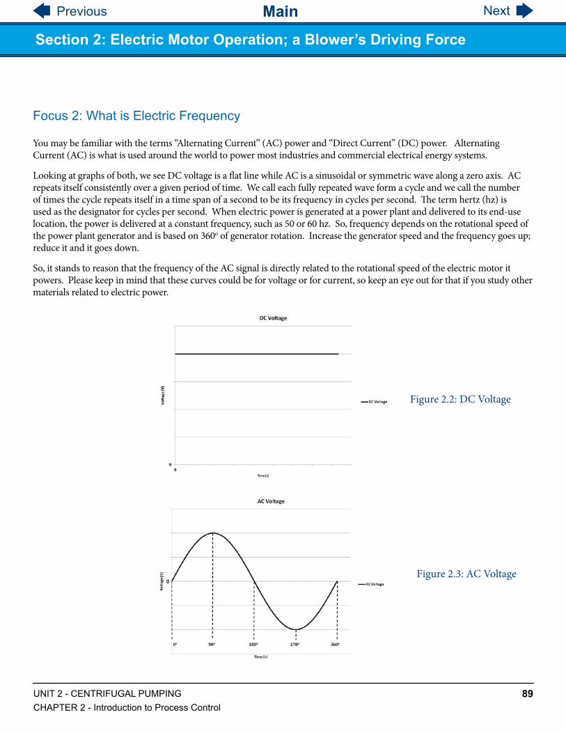
You may be familiar with the terms “Alternating Current” (AC) power and “Direct Current” (DC) power. Alternating Current (AC) is what is used around the world to power most industries and commercial electrical energy systems.

Looking at graphs of both, we see DC voltage is a flat line while AC is a sinusoidal or symmetric wave along a zero axis. AC repeats itself consistently over a given period of time. We call each fully repeated wave form a cycle and we call the number of times the cycle repeats itself in a time span of a second to be its frequency in cycles per second. The term hertz (hz) is used as the designator for cycles per second. When electric power is generated at a power plant and delivered to its end-use location, the power is delivered at a constant frequency, such as 50 or 60 hz. So, frequency depends on the rotational speed of the power plant generator and is based on 360o of generator rotation. Increase the generator speed and the frequency goes up; reduce it and it goes down.

So, it stands to reason that the frequency of the AC signal is directly related to the rotational speed of the electric motor it powers. Please keep in mind that these curves could be for voltage or for current, so keep an eye out for that if you study other materials related to electric power.

Figure 2.2: DC Voltage

Figure 2.3: AC Voltage


Previous Next


Section 2, Focus 2

If your alternating current electrical power source operates as shown in the graphs, what are the frequencies of each power source?

Figure 2.4

Figure 2.5

Figure 2.6


Previous Next


Focus 3: RPM as a Function of Frequency in a Single Phase Motor

If we look at a cross section of simple single phase, 2 pole motor stator (the part that remains stationary), it contains 2 windings (or poles). As the AC waveform that supplies the windings rises from zero to its maximum positive voltage, the upper pole has what is called a north polarity, while the lower one has a south polarity (remember playing with a bar magnet in school, where one end was labeled north and one south-one attracted to a metallic object, one repelled).

When the waveform changes direction and begins to fall, the poles change polarity and then change again when the wave begins to rise again. These polarity changes in the stator send magnetic fields by induction to the motor’s rotor (the part that ultimately turns the motor’s shaft to drive the blower). These magnetic fields oppose magnetic fields already set in the rotor (either by permanent magnets or electromagnets), causing the rotor to spin (hence the name rotor). One AC wave cycle will cause the motor to complete one rotation. So, if the AC frequency was 60 cycles per second (60 Hz), the motor would spin at 60 cycles per second x 1 motor turn per cycle x 60 seconds per minute = 3600RPM. If it was 20 Hz, the motor would spin 1200 RPM.

Figure 2.7: Single Pole Motor

If we increased the number of poles in a motor to 4, the rotational speed of the motor would be half that of the two pole. How’s that? When you wire up 2 more poles in a series configuration, it takes 2 AC power cycles to spin the rotor around the whole stator one time, thus the increase in time to make one full rotation. So, at 60 Hz, the rotational speed would be 60 cycles per second x 1 revolution every 2 cycles x 60 seconds per minute = 1800 RPM. The following handy equation will allow you to compute the rotational speed of a motor if the power supply frequency and the number of motor poles is known:

Section 2, Focus 3

You have a single-phase motor with 6 poles. Your power supply is 25 Hz. What RPM will your motor run?

What will the motor RPM be if you change power supply to 60 Hz?


Previous Next


Focus 4: Three Phase MotorsRemember our discussion about frequency and RPM in a single phase motor. Think back to the poles connected in series. Large power output motors actually have 2 more sets of these poles that are individually wired to be driven by one of three electrical feeds from what is called a three phase power source (verses a single feed from a single phase power source). Simply put, each set of poles is wired in series and are offset from each other by 120o (360o divided by 3) to provide a symmetric application of the sinusoidal wave form. This allows more power to be applied to the motor, thus being able to drive a larger load with a compact motor size. Three phase power has many details which we won’t get into here, but we do recommend checking out other texts on three phase power to gain a deeper understanding. Figure 2.8 shows the 3 sinusoidal wave output of a 3 phase generation system; each wave is displaced from each other by 120o.

Here is what a cross-section looks like for an 8 pole, 3 phase motor. If you look at the stator, you see 8 sets of 3 poles (again, also known as windings or coils). The rotor has 8 windings.

Figure 2.8: Three Phase WaveformSingle Pole Motor

Figure 2.9: Three Phase Motor Cross-SectionSingle Pole Motor


Previous Next


Section 2, Focus 4

You have a 3 phase electric motor with a total of 24 poles in the stator and 8 windings in the rotor. You supply it with 60 hz, 3 phase power. What RPM will your motor run? How about if the power supply was now 50 Hz?

Knowledge Certification Quiz: Section 1 and 2

1. What is process control?

2. Where is process control used?

3. An industrial blower is typically driven by an electric motor. In a process control environment, what is the device that controls the electric motor?

4. An electric motor consists of 2 major parts. Name them and describe their function.

5. Electric power can be provided in what 2 forms? What is the difference between the two?

6. For AC power, what does the term frequency mean? What term designates frequency?

7. What dictates the frequency of electric power?

8. In a 2 pole single phase electric motor, one AC cycle will cause the motor to spin how many revolutions?

9. If the power supplied to the two-pole, single phase motor was 60 hz, what would be the Revolutions per Minute (RPM) of the motor? What if your motor was 4 pole?

10. Single phase AC power has one sine wave. How many does three phase AC power have? How many degrees will each wave offset from each other based on 360 degrees per revolution?

11. If you count up the total number of poles in an 8 pole, 3 phase electric motor stator, how many poles do you actually have? In this instance, how many windings does the rotor have?

12. You have a 3 phase electric motor with a total of 36 poles in the stator and 12 windings in the rotor. Your power supply is 50 Hz, 3 phase power. What RPM will your motor run? What is the motor RPM if you could change the power supply to 70 Hz?

I certify that I have answered all certification quiz questions correctly and am ready for the next lesson.

____________________________________ _____________________________

Your Signature Date


Previous Next


A Little History: Variable Speed (Frequency) Motor Operation

Electric motor operation using a variable electric frequency has been in use for a long time, but the focus back in the early days was on the AC power generator at the power plant. If the generator rotational speed changed, the output frequency followed suit. At that time, frequency changes were limited using this method because the generator still cranked out the same voltage level, but wound up with a higher effective voltage (this is an issue we’ll touch on later in Focus 5). Needless to say, variable speed capabilities for motors were pretty crude and complicated. Back then, a multi-pole motor could be wired to allow switches to vary the number of poles that would be in operation at any given time. The motor’s rotational speed could be changed by manipulating these switches either manually or by some sort of sensor or relay. Other mechanical methods were employed to accomplish speed changes; some so cumbersome as to resemble a “Rube Goldberg” contraption (Never heard of Rube Goldberg? Check it out-you’re in for a treat that will make you smile!).

Today, electronics in the form of a Variable Frequency Drive (VFD) help us to vary the speed of an electric motor with relative ease, while providing excellent precision. In the next section, we will be introduced to the components that make up a VFD and explain their roles in making it work.

Section 3

What was accomplished when poles in the motors were wired so they could be switched on and off during its operation?

Introducing the Variable Frequency Drive (VFD)

As mentioned in the last lesson, the Variable Frequency Drive (VFD) is today’s technology for controlling the speed of an electric motor. A VFD allows precise motor speed control while substantially reducing the blower motor’s electric power requirements. While we could treat a VFD as a black box and just tell you that it works, that wouldn’t be any fun. To get a better feel for what is going on, we will show how this technology works in a step by step fashion. Our remaining discussion will focus on 3 phase motors controlled by a 3 phase VFDs. Figure 3.1: Commercial VFD (left) with electric motor

(Courtesy of ABB Group)

The Heart of Blowing Process Control

In this lesson, the student will learn about the Variable Frequency Drive (VFD), the device which controls the speed of an electric motor at any point of the motor’s operating range.

Approximate Lesson Duration: 1 hr

Section 3: Variable Frequency Drives

Previous Next


Focus 1: Rectifier

As we said earlier, AC power is the predominant power type for numerous reasons. However, it is a difficult task to try to change the frequency of an AC sine wave power source when working with AC. Using Figure 3.1 as a reference, the first thing a VFD does is convert the AC sine wave into a DC wave (A to B) Now, some of this explanation may get a little complicated, but try to stick with it as it will make more sense as everything comes together. The VFD uses an electronic circuit called a diode bridge to limit the travel of the AC sine wave to one direction only (flips all negative waves to positive direction). So, the incoming AC voltage is converted to DC voltage by the diodes. The sine wave changes from a three phase wave to a single wave form . Because the magnitude of the signal is in one direction, a DC circuit thinks it’s a DC signal with “ripples” on the top. So, when a 3 phase VFD accepts 3 separate AC input phases, it converts them to a single DC output.

Figure 3.2: AC Rectifier Circuit

Section 3, Focus 1

The term VFD stands for what?

What does the rectifier in the VFD do?

What is the name of the electric circuit that limits the travel of an AC sine wave to one direction?


Previous Next


Focus 2: Direct Current Bus (DC Bus)

For those new to electricity, the DC Bus is not something you ride on to go to DC, but rather a part of the VFD that uses capacitors and an inductor to filter the AC “ripple” voltage from the converted DC, before it enters a section called the Inverter (next section). If you look at the AC sine wave coming out of the diode bridge, you see that waves all stay positive and the wave is chopped. The capacitor section takes this chopped wave form and smooths out this “ripple” into a controllable DC voltage. It so happens this voltage will be the square root of 2 times the incoming voltage, i.e. a 480 volt system will have a 650-700 volt DC voltage. By the way, the DC Bus also includes filters to prevent something called harmonic distortion that can feed back into the power source supplying the VFD. If you’re not an electrical engineer, don’t fret; this is just some of the “black box” effect the engineers figured out that was needed – just know that it works.

Section 3, Focus 2

What does the capacitor section of the DC Bus do to the wave form that comes out of the rectifier?

Focus 3: InverterThe inverter is the heart of the VFD. It uses 3 sets of high-speed switching transistors to take the output from the DC bus to create DC pulses that look like squared-off versions of the three phases of the AC sine wave (see C in Figure 3.1). These pulses dictate the voltage and frequency of the sine wave. The term inverter or inversion refers to “reversal” and simply refers to the up and down motion of the generated wave form. Today’s modern VFD inverters use a technique known as “Pulse Width Modulation” (PWM) to control or regulate the voltage and frequency (this will be discussed in greater detail in the next section). Within the Inverter is the Insulated Gate Bipolar Transistor (IGBT), which is the actual switching (pulsing) component of the inverter. The IGBT converts the DC voltage from the rectifier/DC bus section back to a “Pulse Width Modulated” (PWM) wave form to send to the motor. The PWM wave form simulates the AC waveform in short pulses. In the electronics world, a transistor can serve 2 functions; it can act as a signal amplifier or as a switch that can simply turn a signal on and off. It features a high switching speed capability while offering lower heat generation. The high switching speeds provide very good AC wave emulation accuracy. This also produces less heat which reduces heat sink cooling requirements and thus provides a smaller package. Since the Variable Frequency Drive controls both the frequency (number of time above and below the zero crossing of the sine waves) and the duration of the on/off, we can send the desired voltage and frequency for the most efficient energy usage. That will be covered next.


Previous Next


Figure 3.3 shows a close up of the wave form generated by the inverter of a PWM VFD overlaid on a true AC sine wave (take a minute to review all that alphabet soup if you’ve forgotten what they stand for).

The inverter output is actually a series of rectangular pulses with a fixed height and adjustable width. In our illustration, there are 3 sets of pulses; a wide set in the middle and a narrow set at the beginning and end of both positive and negative portions of the AC sine wave. If you add up the areas of the pulses, they equal the EFFECTIVE VOLTAGE (which we will cover shortly) of the true sine wave. If we were to chop off the portions above or below the true AC sine wave and use them to fill in the blank spaces under each curve, the result would be almost a perfect match. This is the way a VFD controls voltage going to a motor.

When you add up the width of the pulses and the blank spaces between them, this determines the frequency of the wave (Pulse Width Modulation-PWM) seen by the motor. If the pulse was continuous, without blank spaces, the frequency would still be correct, but the voltage would be much greater than that of the true AC sine wave. The VFD will vary the height and width of the pulse and the width of blank spaces between them to accomplish the desired voltage and frequency. Although it is internally complex, the result is elegantly simple.

One last thing for those who really understand electricity: because this is essentially DC now, people who understand how induction motors work may wonder about how a DC signal can “induce a current” in a motor’s rotor. Without going into detail, just know that the wide DC pulses shown in Figure 3.2 are actually made up of hundreds of individual pulses. This on and off motion of the inverter output allows induction by way of DC to happen.

Focus 4: Output of the Inverter

The inverter takes the output signal from the DC bus and does what with it?

What is the device in the inverter that does that?

What is the technique called which controls or regulates the voltage and frequency?

Section 3, Focus 4

Figure 3.3


Previous Next


As we have seen, AC power is rather complex. If you think about it, one complexity is that it changes voltage continuously; going from zero to some maximum positive voltage, then back to zero, then to some maximum negative voltage and then back to zero. So, how can we tell the actual voltage that is applied to a circuit? Good question!

Figure 3.3 shows a 60 Hz, 120V sine wave. If you look at the peak voltage of the sine wave, it is 170 V. How can this be called a 120V wave if the voltage is 170V? During one cycle, it starts at 0V, rises to 170V and then falls again to 0V. It continues to fall to -170V and then rises back up to 0V. It turns out that the area under the light gray rectangle, whose border is 120V, is equal to the sum of the areas under the positive and negative portions of the curve. Is 120V the average voltage? No. If you average all the voltage values at each point across the cycle, it would yield 108V. Why is it then that a voltage meter will measure 120V? Here is where “Effective Voltage” comes in.

If you were to measure the heat produced by a DC current flowing through a resistor, you would find that it is hotter than the equivalent AC current going through it. This is due to the fact that AC does not maintain a constant value through the cycle (as we have shown). Now, if you did this in a controlled laboratory setting and found that a particular DC current caused a temperature rise of 100 degrees, the equivalent AC circuit would generate a 70.7 degree rise, or about 70.7% of the DC value. Therefore the effective value of the AC is 70.7% of the DC. It also turns out that the effective value of an AC voltage is equal to the square root of the sum of the square of the voltage across the first half of the curve. If the peak voltage is 1 and you were to measure each of the individual voltages from 0 to 180 degrees, the effective voltage would be 0.707 of the peak voltage. So, 0.707 of the peak voltage of 170V is 120V. This effective voltage is also known as the root mean square or RMS voltage. It follows then that the peak voltage will be 1.414 of the effective voltage. So, let’s say you have a measured 230V AC , this would have an effective Voltage of 325V. A measured 460V has a peak voltage of 650V.

Why do we need to know this? Is it just extra torture for no good reason? No. It’s actually meant to give you a better understanding of what a VFD has to go through to work effectively. In addition to varying frequency, a VFD must also vary voltage, even though voltage has nothing to do with the speed an AC motor operates. Stick with this-it will make sense in a minute.

Focus 5: Effective Voltage

Figure 3.4


Previous Next


If you plot a 460V wave form at 50 Hz and then again at 60 Hz, you see a distinct difference (see Figure 3.5). Both have a peak voltage of 650V (1.414 x measured voltage), but the 50 Hz curve spreads out further during the cycle. If you look at the first half of each curve, the 50 Hz curve is larger. Remember when we discussed the area under the curve as being proportional to the effective voltage; this means the effective voltage is higher. This increase in effective voltage becomes even more pronounced as frequency gets smaller. So, if a 460V motor were operated at these higher voltages, it could hurt the lifespan of that motor substantially. Consequently, the VFD must always vary the peak voltage with respect to the frequency in order to maintain a constant effective voltage which the motor is designed to run on. The lower the operating frequency, the lower the peak voltage; the higher operating frequency, the higher the voltage.

This should give you a better understanding of how a VFD controls the speed of a motor. As you will discover, most VFD’s can control a motor speed either manually using a keypad or multi-position switch. They also can be set up to be controlled by sensors (pressure, flow, temperature, level, etc.) to automate the process. So a VFD is a pretty remarkable piece of equipment in terms of what it has to do and what it must keep track of to do it.

Figure 3.5

The term Effective Voltage is also known as what?

Let’s say you have a peak voltage of 500V. What would be your effective voltage for an AC system?

If you are running a peak voltage of 640 V at 60 Hz and decide to have it run at 50 Hz, what happens to the effective voltage? Is this an issue with your motor?

Section 3, Focus 5


Previous Next


Knowledge Certification Quiz: Section 3

1. What does the term VFD stand for?

2. A rectifier in a VFD converts an AC sine wave to what?

3. A diode does what to an AC sine wave?

4. The AC ripple voltage generated by the diode is converted to a DC voltage by what?

5. What does the inverter do?

6. The term Effective Voltage is also known as what?


____________________________________ _____________________________

Your Signature Date


Previous Next


There are essentially 3 situations VFD’s are used for in blowing;

1. Maintain constant pressure

2. Maintain constant flow

3. Provide or react to variable flow

They not only offer a very good way to perform these tasks, but do so with a significant reduction in power consumption over other methods. Let’s use some typical application examples from VFD manufacturers to see how this works.

Focus 1: Constant Pressure

Just as the name indicates, constant pressure is a situation where pressure is maintained at a specific level in the system, even though the flow may be changing. Good examples of constant pressure would be booster blower systems in large commercial and industrial applications. A pressure transducer in the system sends a signal back to the VFD to change blower speed in order to keep pressure constant.

Figure 4.1

In this lesson, the student will look at some examples of typical situations that use Variable Frequency Drives (VFDs) to accomplish objectives.


Section 4: Variable Speed Applications in Blowing

Previous Next


Figure 4.1 is a typical example of a simplex (single) booster blower in a constant pressure application. When you plot the Total Dynamic Head (TDH) of the blower at different operational speeds based on frequency (in our case 60, 55 and 50 Hz), your performance curves map out as shown.

Let’s start with the 60 Hz curve; If you want to maintain a constant head of 120’ (dotted line) at 60 Hz, notice that where those two lines cross yield a flow rate of 150 GPM, while consuming 6.1 HP to do it. This is typically called the “design point”; the maximum flow rate you’ll have to meet while maintaining that constant pressure head.

Now let’s look at the 55 and 50 Hz curves. The dotted horizontal line is still the same constant pressure head to be maintained at the various flow rates. If you look closely, you can see that at about 53 Hz the blower can provide 100 GPM at the design head and at 50 Hz it can provide about 50 GPM. It becomes apparent that over a relatively small frequency range of 50 to 60 Hz, the blower will provide 50 to 150 GPM at 120’. Remember that the VFD produces not only 50, 55, and 60 Hz pulses, but also each individual (and fractional) Hz in between. It can settle on the optimum frequency for the particular need. This yields a significant savings in the power required if the flow requirements drop lower than the “design point” flow. The brake BHP requirement at 53 Hz (100 GPM) drops to 3.8 or 58% of design point HP. At 50 Hz (50 GPM), it drops to 2.4 HP or just 39% of that at the design point.

Now, we could use a pressure reducing valve (PRV) to maintain a constant pressure of 120 feet as flow demand decreases and take advantage of the centrifugal blower’s reduced power consumption as its flow moves towards the left of the capacity curve (remember, we are on the 60 Hz curve when we do this). But, at the 100 GPM point on the 60 Hz curve the power requirement is 5.2 HP (compared to only 3.8 HP if we lowered the operating frequency down to approximately 53 Hz). At 50 GPM, the PRV control requires 4.1 HP on the 60 Hz curve, or 72% more than an optimized VFD frequency. In a constant pressure application, the VFD offers precise and flexible control plus an increased power savings over mechanical constant pressure devices. Because centrifugal blowers follow the laws of affinity, a relatively small change in frequency (speed) can result in a substantial reduction in power.

If you have not studied the affinity laws for centrifugal blowers, they state that;

1. Capacity varies directly as the change in speed

2. Head varies as the square of the change in speed

3. Brake horsepower varies as the cube of the change in speed.

1. For a constant pressure flow situation, can the flow be changing and still achieve constant pressure?

2. What do you call the maximum required combination of pressure and flow for this situation?

3. If you can back off of flow while still maintaining the pressure design point, can a VFD be useful in this situation? Would a Pressure Reducing Valve (PRV) work better? Why?

Section 4, Focus 1


Previous Next


Figure 4.2 shows a constant flow application (vertical line at 50 Gallons per Minute). These applications require flow to remain constant regardless of the pressure fluctuations the system may encounter. A flow meter is usually employed to control VFD output and, in turn, motor speed. Examples of constant flow include maintaining levels in tanks at various elevations, manufacturing processes, and the operation of nearby and remote irrigation zones. Each of the multiple components served by these applications require similar flows but, differences in elevation, back pressure, and pipe line friction may require different pressures to maintain those flows. The system is designed for the highest pressure component of the application so that the VFD can reduce motor speed for the lower pressure component and save energy in doing so. Otherwise, a throttling valve that kept flow constant based on pressure would be in use. Motor electrical consumption would remain similar to the set point usage. If you examine the graphed blower curves closely, just like you did for the constant pressure analysis, you will see the opportunities presented when pressure does not have to be maintained at one specific “design point” to maintain the flow set point.

Focus 2: Constant Flow

Figure 4.2

1. Can you name three constant flow applications?

2. What types of situations cause challenges to maintaining steady flow?

3. If you didn’t have a VFD, what less sophisticated means of controlling flow would you have to use? What is one major problem with using it?

Section 4, Focus 2


Previous Next


Variable Flow applications might also be called variable flow / variable pressure because neither remains constant. For your information, most are circulation applications and deal only with pipe line friction as flow changes. A major application area is that of chilled water circulation in large air conditioning systems (HVAC) where cooling demand is always changing. Since the chilled water flows in a circulation loop, the only pressure component that changes is that due the friction caused by the flowing water. VFD output is controlled by a flow meter, temperature transmitter, or directly by the chiller controls. The cooling tower blower is often controlled by the same circuit.

Focus 3: Variable Flow

Figure 4.3 is a depiction of a variable flow, chilled water application. The straight upwardly-sloped line shows flow points on the various frequency curves and the additional pressure (in Head) required to over-come friction as flow increases. Please note that the straight line could be curved depending on the design. Since friction is not a linear function, it may have some curvature based upon the calculated friction in the circulation loop. In the past, multi speed motors were used for this application. Large swimming pools also use a similar design for circulation through a filter. Again, power savings are achieved as the flow is decreased by the VFD.

Figure 4.3

A final advantage that will be touted in VFD application benefits is the Soft Start/Stop option. This option allows the blower and motor to be started at a lower frequency (say 30 hz) and then “ramped” up to run speed over a period of a second or more. The result is a significant reduction in the starting current required by the motor, verses it just starting and ramping right up to 60 Hz. Equate it to stomping your engine throttle to the floor verses gently pushing on it to slowly ramp up your speed. The former requires much more energy input all at once and creates more stress than the latter. Some utilities require that motors over a certain HP undergo a soft start. With the VFD, it’s just part of the package. In addition to a lower inrush current, mechanical stress on the motor and blower are also greatly reduced. In a normal “across the line” start, the motor rotor and blower rotating element go from motionless to the motor’s rated RPM in about one second! And, soft start/stop virtually eliminates a phenomenon called water hammer in almost any blowing system (you might want to read up on that).

Focus 4: Soft Start


Previous Next


1. Variable flow situations are mainly concerned with what 2 issues?

2. Can you name a situation where variable flow control is needed?

3. What typically can be used in a variable flow application if a VFD is not used?

4. Can you describe what a motor soft start is?

Lesson 4, Focus 3 and 4

Knowledge Certification Quiz: Lesson 4

1. Name 3 situations where VFDs are used in fluid blowing.

2. In a “constant pressure” fluid blowing scenario, what feedback sensor is used to “talk” with the VFD?

3. In a “constant flow” fluid blowing scenario, what feedback sensor is used to “talk” with the VFD?

4. What happens to a blower performance curve if the driving frequency is lowered?

5. In a variable flow blowing scenario, can both pressure and flow be changing at the same time?

6. Name an application that has variable flow requirements.

7. What does the term “soft start” mean regarding electric motors?


____________________________________ _____________________________

Your Signature Date


Previous Next


Way back in Lesson 1, we gave a general definition for Process Control:

Process control is the ability to manipulate or control some form of operation on a consistent basis to produce reliable desired outcomes. In blowing, this means controlling a blower to produce desired flow and/or pressure results in the system in which it is operating. This usually means the system environment offers “feedback” information to the blower so that it can automatically adjust how it runs in order to properly meet the needs of the situation.

We want to expand this discussion to show how processes differ in necessary control schemes to get the job done most efficiently. This means we will look at ever increasing capabilities to fill a need. We’ll use various examples from different scenarios to make the point, but will use this building block knowledge to ultimately focus on blowing fluid.

Focus 1: Open Loop Control: A Return to Watering the Lawn

Remember in lesson 1 when we talked about adding the sprinkler system to your lawn? When it was strictly operating on a timer, which turned it on and off at preset times (even if it was raining outside), the “process” environment this control scheme worked in is known as “open loop” control. Open loop control works well as long as the event it controls is repetitive and no damage could result from its action. If your sprinkler activates while it’s raining, the water is wasted but no damage occurs. Open loop controls are also simple and inexpensive. The key characteristic of open loop control is that the controller has no clue what is going on within the system. It simply follows its instructions, to the letter, regardless of its surroundings.

Focus 2: Closed Loop Control: The Heating System

While the lawn sprinkler can run relatively well in an open loop manner, your home heating system would not. If open loop control was used, you would experience times when it was too warm and others when it was too cold as the heater would start and stop based on a simple timer cycle. To combat this problem you need “feedback” to the heater based on the desired temperature and the actual measured temperature at any point in time. Your heating system could then make its own decision when to start and how long to run. In the typical home heating system, this is accomplished with a thermostat. When the temperature drops below a certain predetermined level, the thermostat starts the heating system and runs it at its full capacity until the temperature rises to the thermostat setting. The thermostat then stops the heating system and waits to begin another cycle. This is a simple example of “closed loop” control. More specifically, it is known as “on/off, closed loop control” as the heater is either fully on or fully off and there are no intermediate settings. The key characteristic of the closed loop controller is that it receives some form of feedback as to what is going on within the system and can therefore make more “intelligent” decisions. The downside is that when you look at an operational graph of the system, you see that it is not very precise. If it’s above the desired temperature, it shuts off; if below, it turns on. This looks something like Figure 5.1.

In this lesson, students will expand their knowledge of Lesson 1 to better understand the logic of Process Control in blowing.


Section 5: Process Control Logic

Previous Next


To take this discussion a little further. This type of control is known as Dead Band control. The controller allows the signal to oscillate between a low and high set point (the Dead Band) so that the furnace isn’t constantly turning on and off for short durations. When the low set point is reached, the controller calls for an increase. When it reaches the high set point, it calls for a decrease. Now, the problem with this is that there is usually a delay between the time the final control element changes (in this case, temperature) and the time the sensor reads the measurement (called PV or Process Variable). This delay is called lag time and unless the sensor is very fast, the control element very responsive and the physical distance between them is very short, the measured values will both overshoot the high and low set points. Many methods have been tried to remediate the problem and these schemes are called control algorithms. The most common control algorithm is PID; Proportional, Integral and Derivative control. The Proportional value determines the reaction to the current error. The Integral Value determines the reaction based on the sum of the recent errors. The Derivative value determines the reaction to the rate at which the error has been changing. The output of the controller to the final control element is the weighted sum of these 3 values.

Figure 5.1

Focus 3: Getting a Better Feel for Controller Logic (Hand-Controlling the Process).

Let’s think about something you’re very familiar with; controlling water temperature using hot and cold faucets. You turn these on and touch the water to feel the temperature. Based on the feedback, the faucets are adjusted until the water reaches the desired temperature.


Previous Next


Touching the water is what we call a process variable-it’s the difference between what the temperature of the water currently is and what we want it to be. In control lingo, this difference can be called the error. You determine that the water is too hot or too cold and also by how much.

Knowing the magnitude of the error, you change the faucet positions. When you first do this, you might turn the hot valve on just slightly if you want warm water; or you may turn it on full-blast if you want very hot water. You’re doing this in relation or proportion to how far off you think the temperature is from where you want it to be. Keep this in mind as this will be something we will be talking about later called Proportional Control. Now, if the hot water isn’t coming fast enough, you may try to speed up the process by opening the hot water valve more, checking temperature, and doing this more as time goes by. You’re in essence looking at the past history of how the temperature was changing based on your input and adjusting it quicker. This would be an example of Integral Control.

Now, if you make too big a change when the error is small, you can overshoot your target (water gets too hot). If you kept doing this, (being ham-handed, without good control over yourself) you would repeatedly overshoot your goal. If you think about it in a graphical form, you would create a wavy pattern that would oscillate around the set-point temperature. If the oscillations increase as time goes on, you have what’s called an unstable system (and an unstable operator). If they remain at a constant level or decrease, the system is considered marginally stable.

If you have some finesse and control, you want to gradually converge your faucets so the desired water temperature is reached. You do this by settling down or tempering your ham-handed oscillations (being in tune with rate of change you are applying to the faucets) as you move forward. This can be thought of as an example of Derivative control.

Once you get it the way you want it (zero error), no changes will need to be made unless the system experiences a disturbance. Maybe someone else just turned on their faucet next to you and is using some of your warm water stream, which makes yours cooler. This increases your error and you have to react. This is the way a controller functions in industry.

After going through all of that, the good news is that a PID Controller can successfully replace the human being. Whew! We’ll talk about that next.

1. What is the main difference between open-loop control and closed-loop control?

2. When your heating thermostat is set at 70, but your room temperature is 65, what is this difference known as?

Section 5


Previous Next


ControlsLabTM uses something called a Proportional-Integral-Derivative Controller, or PID for short, to control the on-board Variable Frequency Drive (VFD) which ultimately controls the speed of the motor driving our blower. This PID controller changes the speed of the blower, in very specific ways, after receiving “feedback” from the system in which the blower is operating in. How this works and why this is important is what we want to learn now. Let’s ease into this a step at a time as we build toward a quality understanding of PID Control. A proportional-integral-derivative controller (PID controller) is a common control-loop feedback controller widely used in industrial control systems.

When a process loop is created by adding feedback (from a variable such as airflow, pressure, or level) and sent to the VFD, regulation of the variable is possible through the PID loop control. A PID controller calculates an “error” value; the difference between what we are measuring in the process (process variable) and our desired setting (set-point).

The VFD’s PID controller determines the proper reaction to the error; the changes between the system set-point and its actual state as measured by feedback. The controller attempts to minimize the error by adjusting the process control inputs.

Knowledge Certification Quiz: Section 5

1. How could you convert a yard light from an “open loop” control to a “closed loop” control?

2. What does an ON-OFF Control Loop mean?

3. Does an ON-Off Control Loop maintain an accurate set-point result? Why or Why Not?

4. Referring to the controlling water temperature with your hand example in the text, list 2 other processes that would work similarly.


____________________________________ _____________________________

Your Signature Date

Focus 1: PID Control Overview

Section 6: The PID Controller

(The Brains and Logic of Blower Process Control)

In this lesson, the student will learn about the PID control algorithm for process control and its functionality.




Previous Next


Figure 6.1 shows a basic schematic diagram of a closed-loop system using a feed-back controller to control error.

Figure 6.1: Block diagram of a closed loop control system. The basic premise of this scheme is to adjust the motor conditions in order to minimize the error signal.

The PID controller logic consists of an algorithm (a programmed calculation formula for solving a problem in a finite number of steps), that has three separate constant parameters: the proportional, the integral and derivative values, denoted P, I, and D. Basically, these values can be interpreted in terms of time: P depends on the present error, I on the accumulation of past errors, and D is a prediction of future errors, based on current rate of change. The weighted sum of these three actions is used to adjust the process via a control element such as the position of a control valve, a damper, or the power supplied to a heating element. In the case of ControlsLabTM, this is used to control the speed of the blower and is accomplished through a software program that is executed by a PAC (programmable automation controller) built into the VFD. You may also hear algorithms being referred to as instructions, procedures, functions or programming. The general control algorithm is laid out as follows:

Figure 6.2: General PID Control Algorithm


Previous Next


Figure 6.3: Proportional Control Error

1. Is a PID controller meant for open or closed loop operation?

2. Does a PID controller need any feedback to work effectively? Why?

3. What is an algorithm?

Section 6, Focus 1

Furthermore, by tuning the three parameters with something called Gain in the PID controller algorithm, the controller can provide control action designed for specific process requirements (we’ll talk more about Gain shortly). The response of the controller can be described in terms of how the controller responds to an error, the degree to which the controller overshoots the set-point and the degree of system oscillation. Please note that the use of the PID algorithm for control does not guarantee optimal control of the system or system stability. You try to get it tuned to be the most effective over the full course of operation. Let’s get into more detail about how each element we discussed works.

Looking at Figure 6.3, the black line plots the proportional signal trying to react to a change in an input signal in order to maintain a set point (zero line). You see that it shoots upward, overshoots, turns toward the set point, then undershoots. It continues this pattern in a diminishing fashion until it is settled on the set point.

The integral function measures the areas under the curves (errors) and the derivative function measures the rate of change of that curve as it moves along to the right. In essence, these two functions measure how much error the proportional algorithm has in getting to the set point for this application and uses that information to apply measures to speed up the proportional signal response and to reduce that error. We’ll explore each element of PID in greater detail next.


Previous Next


Focus 2: Proportional Control (The P in PID)

Remember how you added control elements to your lawn sprinkler to get it automated and react intelligently to the current lawn moisture situation? Let’s take a similar approach with your heating system.

Your old home heating system used a basic closed loop, on/off thermostat, as described earlier. One day the old furnace died, so you had the local dealer install a brand new one. He brought you up to speed on the latest technology and showed you that the new thermostat can transmit the actual measured temperature in the room back to the heating system controller. He also showed you that your new heating system can vary its output based upon the temperature it receives from the thermostat. In your case, your new furnace has 4 gas burners that can be controlled so only one or two burners can be operating (an electric furnace could control a number of heating elements). A variable speed fan in the unit also helps the control of heat.

As the temperature in the room approaches its’ “set point” the heater would not necessarily turn off but, instead, reduce its output (turn off some burners) and attempt to keep the room at the desired temperature. If the temperature drops, it would increase its output (turn on more burners) and if the temperature increases it would either reduce its output or shut off completely. Furthermore, these changes in output would be in “proportion” to the change in temperature. A small change in temperature results in a small change in output while larger changes in temperature would lead to proportionally larger changes in heat output. The heating system example is one of “proportional, closed loop” control and is the “P” in “PID”. Figure 6.4 shows how the proportional control smoothly changes the system output to get the existing low temperature back to the desired set-point. (Notice that it doesn’t quite make it to the set point. This is known as offset in industry and is one of the reasons we need more than proportional control to effectively establish the best results in process control. This will be addressed in the next section.

Figure 6.4: Proportional Control Curve


Previous Next


Proportional control is used in systems where the feedback measurement tends to change slowly. Another example you may be familiar with is your car’s cruise control-it also operates by proportional control. The controller monitors your speed and changes the throttle setting in proportion to the change in speed it sees. These devices work very well on level and slightly inclined roads but you have probably noticed that they do not work as well on a steep incline. A steep incline will decrease your speed quickly but the controller reacts in its normal fashion and speed will remain well below the set point until, ultimately, the transmission drops into a lower gear and the speed set point is once again reached. If the steep incline continues, this cycle will repeat itself a number of times.

Proportional control is very common for blowers used in process plants. Some processes use a grouping of blowers that can collectively or individually come on or drop off to adjust output based on what is needed. Multiple blower booster systems use multiple pressure switches to bring additional blowers on line based upon changes in system pressure.

Figure 6.5: Proportional Component (with Gain Factor) of PID Control Algorithm

Looking at formula in Figure 6.5, the proportional term produces an output value that is “proportional” to the existing error being experienced by the system. The proportional response can be adjusted by multiplying the error by a proportional gain constant.

A high proportional gain can result in a large change in the output for a given change in the error. If it’s too high, the system can become unstable; too low and the reaction might not be adequate enough, especially if your system does experience a disturbance. Based on theory and industrial practice, the proportional part of the PID controller should contribute the majority of the output change.


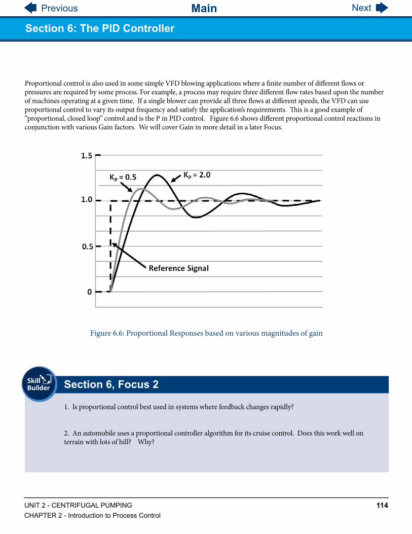
Previous Next


Proportional control is also used in some simple VFD blowing applications where a finite number of different flows or pressures are required by some process. For example, a process may require three different flow rates based upon the number of machines operating at a given time. If a single blower can provide all three flows at different speeds, the VFD can use proportional control to vary its output frequency and satisfy the application’s requirements. This is a good example of “proportional, closed loop” control and is the P in PID control. Figure 6.6 shows different proportional control reactions in conjunction with various Gain factors. We will cover Gain in more detail in a later Focus.

Figure 6.6: Proportional Responses based on various magnitudes of gain

1. Is proportional control best used in systems where feedback changes rapidly?

2. An automobile uses a proportional controller algorithm for its cruise control. Does this work well on terrain with lots of hill? Why?

Section 6, Focus 2


Previous Next


Focus 3: Integral Control (The I in PID) If changes in your process are gradual and there’s lots of time for Proportional Control to react, then proportional control usually works great. But most of the time, changes occur fairly quickly (maybe even abruptly); proportional can’t respond fast enough or with the right magnitude. It tries, but inevitably it can’t keep up, and starts over-reacting. This creates instability in the process to the point where the process losses control. In this situation, the proportional control algorithm needs some assistance. One of these assists is provided by Integral Control.

In blowing applications, proportional control is usually satisfactory to maintain the flow requirements if conditions are fairly steady, with no sudden changes and if small offsets are tolerable.

Proportional control, by itself, is not dependent on time in a control process. Consequently, the process usually will reach a steady state condition where the error signal just stays there and doesn’t change with time. In other words, the controller output would never bring the controlled variable exactly equal to the setpoint. You would always have some small amount of error. This is often called offset. Offsets are steady state errors that proportional control can’t overcome alone. The Integral term senses this long term offset, and corrects the controller output to reduce the effect of offset (return to Figure 6.4).

The contribution of the integral term is proportional to “how big the error is and how long it lasts”. It adds up all the instantaneous errors (areas under the curves-errors) over time and corrects the offset the system experiences with proportional-only control. A gain factor is applied to affect how the controller reacts.

Keep in mind that in a typical process, a VFD is tasked to respond to a single condition, such as a change in pressure or flow in the system. It is usually fed a signal from a pressure or flow transducer strategically placed to tell the VFD what the situation is so it can adjust its operation to maintain a required set point.

Figure 6.7: Integral Component (with Gain Factor) of PID Algorithm


Previous Next


The integral term accelerates the movement of the process towards the setpoint and eliminates the steady-state error (offset) that occurs with a proportional-only controller. Integral gain can be set to change how quickly the integral response occurs. Figure 6.8 shows 2 different responses to a desired set point; one responds gradually and meets the set point curve smoothly, the other responds much more quickly, but overshoot and oscillates until it settles on the set point.

Figure 6.8: Integral responses based on various magnitudes of gain

1. Integral Control assists Proportional Control by doing what?

Section 6, Focus 3


Previous Next


Focus 4: Derivative Control (The D in PID)The derivative responds to the rate of change of the process error (take a moment and think about that). It reduces overshoot of the process control during sudden large disturbances. The differential element is only responsive during transient conditions (when conditions change) and is not active for steady state errors because their rate of change is zero. Just like with proportional and integral functions, applying a gain factor to the derivative function results in different responses.

Figure 6.9: Derivative component (with Gain Factor) of PID Algorithm

Figure 6.10: Derivative responses based on various derivative gain factors.


Previous Next


1. What does the derivative portion of the control algorithm respond to?

Section 6, Focus 4

Figure 6.11: Closed loop control system showing the three components of PID control output.

If we look at Figure 6.11, it shows a full PID algorithm imbedded in a control loop. All 3 elements can contribute to controlling errors in the system, which is depicted in Figure 6.12.

Focus 5: Putting It All Together: PID Control


Previous Next


Figure 6.12: A system response using PID Control

Interestingly enough, in most blower applications, proportional and integral control (PI control) is sufficient for maintaining process control. The proportional control will amplify the output in proportion to the error signal and the integral control amplifies the output based on the accumulation of error with time. Proper selection of the gains for these two control elements is critical to the success of any closed loop control application. Figure 6.13 shows the response curves of the ControlsLabTM centrifugal blower system when reacting to a step change of the pressure setpoint using differing values of proportional and integral gain. In this figure, the importance of proper gain settings is easily recognized. Imagine a traffic cop monitoring the flow of traffic (in this situation, the proportional algorithm of the VFD controller) with his or her radar gun, trying to keep it from speeding off in one direction or another. You may like to refer to it as the “how much function”. It does this by keeping track of the errors that occur and using that information to correct those errors in the future. Almost every time a VFD attempts to bring a change in system pressure back to the set point, it makes a mistake; that is, it initially misses the set point. There are many reasons for this; the way the algorithm was written for the application, data sampling rate, etc.

Figure 6.13: Pressure response of the ControlsLabTM to a step change in the pressure setpoint using differing values of the proportional and integral gain.


Previous Next


1. What is the basic job of the Integral and Derivative functions?

2. What does the integral function do?

3. What does the derivative function do?

Section 6, Focus 5


1. What is a control algorithm?

2. What is the primary attribute of proportional control?

3. What is the primary attribute of integral control?

4. What is the primary attribute of derivative control?

5. Can you have just a proportional algorithm for control?

6. Name a common proportional algorithm application.


____________________________________ _____________________________

Your Signature Date


Previous Next


In this lesson students will learn about applying Gain to a control algorithm to optimize response.

Focus 1: Introduction to Gain

As we have discussed, the response of each PID control element can be adjusted by multiplying the error for each control element by a constant called gain. This constant can be changed during the operation of the system until the optimum response is reached. In the PID algorithm, the K elements signify the gain factors

The process of setting the optimal gains for P, I and D to get an ideal response from a control system is called tuning. There are different methods for tuning a PID loop, including; manual tuning (also known as a trial and error method), the Ziegler Nichols method, and tuning software.

Figure 7.1: Control Algorithm

Focus 2: Manual Tuning-Trial and Error

The gain settings of a PID controller can be obtained by trial and error method. Once an engineer understands the significance of each gain parameter, this method becomes relatively easy. In this method, the I and D gain terms are set to zero first and the proportional gain is increased until the output of the loop oscillates (does not settle). As one increases the proportional gain, the system becomes faster, but care must be taken not make the system unstable. Once P has been set to obtain a desired fast response (with oscillations), the integral term is increased to stop the oscillations. The integral term reduces the steady state error, but increases overshoot. Some amount of overshoot is always necessary for a fast system so that it could respond to changes immediately. The integral term is tweaked to achieve a minimal steady state error. Once the P and I have been set to get the desired fast control system with minimal steady state error, the derivative term is increased until the loop is acceptably quick to its set point. Increasing the derivative term decreases overshoot and yields higher gain with stability but would cause the system to be highly sensitive to noise. Often times, engineers need to trade-off one characteristic of a control system for another to better meet their requirements.


Section 7: Tuning Methodologies-An introduction to Gain

Previous Next


Focus 3: The Ziegler-Nichols MethodThe Ziegler-Nichols method is another popular method of tuning a PID controller. It is very similar to the trial and error method wherein I and D are set to zero and P is increased until the loop starts to oscillate. Once oscillation starts, the ultimate gain Ku and the period of oscillations Tu are noted. The P, I and D are then adjusted as per the tabular column shown below.

Focus 4: PID Tuning SoftwareModern process facilities, especially with complex processes, can also utilize PID tuning and loop optimization software to ensure consistent results. These software packages will gather the data, develop process models of the system and suggest optimal tuning. There are a variety of programs available, including custom application developments.

Table 7.1- Ziegler-Nichols tuning, using the oscillation method

1. Can you name three methods of applying gain to a PID process?

2. Can you just use P&I in a control system to get adequate control?

Section 7


1. What is gain?

2. What is the process called of setting optimal gains to get the desired control responses?

3. What does gain improve for each element of the control algorithm


____________________________________ _____________________________

Your Signature Date

Section 7: Tuning Methodologies-An introduction to Gain

Previous Next

123

172.23.120.70 172.23.120.65

172.23.120.67

172.23.120.xx

172.23.120.xx

172.23.120.xx

172.23.120.1HMI PAC

VFD

Wireless172.23.120.1

Unit 3 - Ethernet Communication

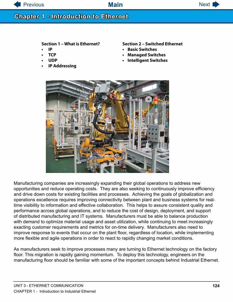
Previous Next

124UNIT 3 - ETHERNET COMMUNICATIONCHAPTER 1 - Introduction to Industrial Ethernet

Chapter 1 - Introduction to Ethernet

Manufacturing companies are increasingly expanding their global operations to address new opportunities and reduce operating costs. They are also seeking to continuously improve efficiency and drive down costs for existing facilities and processes. Achieving the goals of globalization and operations excellence requires improving connectivity between plant and business systems for real-time visibility to information and effective collaboration. This helps to assure consistent quality and performance across global operations, and to reduce the cost of design, deployment, and support of distributed manufacturing and IT systems. Manufacturers must be able to balance production with demand to optimize material usage and asset utilization, while continuing to meet increasingly exacting customer requirements and metrics for on-time delivery. Manufacturers also need to improve response to events that occur on the plant floor, regardless of location, while implementing more flexible and agile operations in order to react to rapidly changing market conditions.

As manufacturers seek to improve processes many are turning to Ethernet technology on the factory floor. This migration is rapidly gaining momentum. To deploy this technology, engineers on the manufacturing floor should be familiar with some of the important concepts behind Industrial Ethernet.

Section 1 – What is Ethernet?• IP• TCP• UDP• IP Addressing

Section 2 – Switched Ethernet• Basic Switches• Managed Switches• Intelligent Switches

Previous Next


Section 1: What is Ethernet?

Focus 1: Types of EthernetLocal Area Networks (LANs)A network is any collection of independent computers that exchange information with each other over a shared communication medium. Local Area Networks or LANs are usually confined to a limited geographic area, such as a single building or a college campus. LANs can be small, linking as few as three computers, but can often link hundreds of computers used by thousands of people. The development of standard networking protocols and media has resulted in worldwide proliferation of LANs throughout business and educational organizations.

Wide Area Networks (WANs)Often elements of a network are widely separated physically. Wide area networking combines multiple LANs that are geographically separate. This is accomplished by connecting the several LANs with dedicated leased lines such as a T1 or a T3, by dial-up phone lines (both synchronous and asynchronous), by satellite links and by data packet carrier services. WANs can be as simple as a modem and a remote access server for employees to dial into, or it can be as complex as hundreds of branch offices globally linked. Special routing protocols and filters minimize the expense of sending data over vast distances.

Wireless Local Area Networks (WLANs)Wireless LANs, or WLANs, use radio frequency (RF) technology to transmit and receive data over the air. This minimizes the need for wired connections. WLANs give users mobility as they allow connection to a local area network without having to be physically connected by a cable. This freedom means users can access shared resources without looking for a place to plug in cables, provided that their terminals are mobile and within the designated network coverage area. With mobility, WLANs give flexibility and increased productivity, appealing to both entrepreneurs and to home users. WLANs may also enable network administrators to connect devices that may be physically difficult to reach with a cable.

Previous Next


Focus 2: Types of LAN Technology

Ethernet is by far the most widely used LAN technology today. It is estimated that more than 85 percent of the world’s LAN connected PCs and workstations use Ethernet. Ethernet refers to the family of computer networking technologies covered by the IEEE 802.3 standard, and can run over both optical fiber and twisted-pair cables. Over the years, Ethernet has steadily evolved to provide additional performance and network intelligence. This continual improvement has made Ethernet an excellent solution for industrial applications. Today, the technology can provide four data rates.

● 10BASE-T Ethernet delivers performance of up to 10 Mbps over twisted-pair copper cable.

● Fast Ethernet delivers a speed increase of 10 times the 10BASE-T Ethernet specification (100 Mbps) while retaining many of Ethernet’s technical specifications. These similarities enable organizations to use 10BASE-T applications and network management tools on Fast Ethernet networks.

● Gigabit Ethernet extends the Ethernet protocol even further, increasing speed tenfold over Fast Ethernet to 1000 Mbps, or 1 Gbps. Because it is based upon the current Ethernet standard and compatible with the installed base of Ethernet and Fast Ethernet switches and routers, network managers can support Gigabit Ethernet without needing to retrain or learn a new technology.

● 10 Gigabit Ethernet, ratified as a standard in June 2002, is an even faster version of Ethernet. Because 10 Gigabit Ethernet is a type of Ethernet, it can support intelligent Ethernet-based network services, inter-operate with existing architectures, and minimize users’ learning curves.

To date, more than 300 million switched Ethernet ports have been installed worldwide. Ethernet technology has a wide acceptance because it is easy to understand, deploy, manage, and maintain. Ethernet is low-cost and flexible, and supports a variety of network topologies. Compared to traditional, non-Ethernet-based industrial solutions that have a data rate of between 500 Kbps to 12 Mbps, Ethernet technology can deliver substantially higher performance. It is based on industry standards, and it can connect over any Ethernet-compliant device from any vendor.


Previous Next



Focus 3: IP (Internet Protocol)

IP is often understood as the Internet Protocol suite: A suite of protocols and standards on which the Internet and most enterprise networks are based. The IP suite includes not only lower-level specifications, such as TCP and IP, but specifications for such common applications as e-mail, terminal emulation, and file transfer. The most relevant of these to the factory floor though are IP itself, TCP, and UDP. These three protocols communicate in collaboration to form what is known as the Internet. This technology is moving automation forward, giving operators the ability to access and control plants remotely.

IP is the common and primary network (Layer 3) protocol in the Internet suite. IP represents the core of the Internet Protocol suite. It defines an address by which the network can transmit the packet from source to destination—even across LANs. This is opposed to the MAC addresses, which are used to network locally, within a LAN. IP has two primary responsibilities: providing connectionless, best-effort delivery of datagrams or packets through a network; and providing fragmentation and reassembly of datagrams to support data links with different maximum-transmission unit (MTU) sizes. More on IP address allocation and administration is found in the network management section.

Previous Next


Focus 4: TCP (Transmission Control Protocol)

TCP provides reliable, in-order delivery of packets between two devices. It relies upon IP. TCP applications establish connections between one another over which they send packets. TCP is a stateful protocol; it maintains the state after the packet is sent. TCP checks whether all packets have arrived and can request re-transmission if a packet is dropped, lost, or corrupted during transmission. Due to this overhead though, TCP is not always ideal for realtime applications. TCP has emerged as the dominant protocol used for the bulk of Internet connectivity. Its services break large data sets into individual packets, checking for and resending lost packets and reassembling packets into the correct sequence. But these additional services come at a cost in terms of additional data overhead, and delays called latency.

TCP is a connection-oriented protocol, which means a connection is established and maintained until the application programs at each end have finished exchanging messages. It determines how to break application data into packets that networks can deliver, sends packets to and accepts packets from the network layer, and manages flow control. It is meant to provide error-free data transmission. If any data packets get dropped or garbled, they will re-transmit until acknowledgment that all packets arrived sucessfully. This error-free feature requires a complicated routine. Below is a diagram showing the TCP routine.


Previous Next


Focus 5: UDP (User Datagram Protocol)

UDP is often used for real-time communications such as voice and I/O traffic. UDP also relies on IP. UDP does not guarantee delivery or the order of the packets, thus simplifying the protocol. It has much lower bandwidth overhead and latency. The applications would rather drop a packet than receive it late. UDP is considered a “stateless” protocol. It is compatible with packet broadcast (sending to all on local network) and multicasting (sending to all subscribers). UDP is an ideal protocol for network applications in which perceived latency is critical such as gaming, voice and video communications, which can suffer some data loss without adversely affecting perceived quality. In some cases, forward error correction techniques are used to improve audio and video quality in spite of some loss.

UDP can also be used in applications that require lossless data transmission when the application is configured to manage the process of retransmitting lost packets and correctly arranging received packets. This approach can help to improve the data transfer rate of large files compared with TCP. The main goal for UDP transmission is send it as fast as possible. The diagram below summarizes UDP transmission:


Previous Next


Focus 6: IP Addressing

Establishing policy and managing the IP addresses are relevant to a control engineer. Typically, any Industrial Ethernet device (new or replacement) needs an IP address assigned to it. Many production facilities use statically assigned addresses where someone has to decide the address and configure end devices with their IP addresses. As most automation and control applications use the IP address directly in their programs, this is a straightforward way to make sure they stay in-sync, although as a facility grows, it can become a maintenance burden. Therefore, some facilities use dynamically administered IP addresses, where every time the device starts, it gets its IP address from a network service, for example using the Dynamic Host Configuration Protocol (DHCP). The network service can be configured to issue consistent IP addresses so automation and control programs do not have to be changed, provided the appropriate network design and configuration. Lastly, control engineers should also ensure they get enough IP addresses allocated and have an allocation method that allows factory floor devices to be easily recognized. IT is usually responsible for allocating enterprise IP addresses.

1. Typical networks use Gigabit Ethernet. How does this speed compare to traditional non-Ethernet speeds?

2. What Ethernet protocol doesn’t guarantee packet delivery?


Previous Next


Section 2: Types of Switched Ethernet

Focus 1: Basic Switches

Organizations can choose from a variety of devices and architectures when building an Ethernet LAN. Devices range from simple hubs, to unmanaged switches, to intelligent, managed switches. The network components are important to the proper functioning of the automation network, and careful consideration should be given to selecting the appropriate device.

Early Ethernet deployments often used hubs. Hubs act at the physical layer of the OSI model, and are essentially repeaters that connect multiple devices over the same shared medium. Because hubs use a shared medium, collisions can occur when multiple devices try to communicate at the same time. This may not be a significant concern in a small network without high-performance requirements, but is typically not acceptable in environments where real-time, predictable performance is important, such as automation networks. The collisions that resulted from the use of hubs contributed to the perception that Ethernet is not deterministic, even though hubs are rarelyused anymore.

Over the past 10 years, most Ethernet deployments have used full-duplex switched Ethernet switches. Switches make it possible for several users to send information over a network at the same time without slowing each other down. In a fully switched network, there are no hubs so each Ethernet network has a dedicated segment for every node. Because the only devices on each segment are the switch and the node, the switch picks up every transmission before it reaches another node. The switch then forwards the data over to the appropriate segment. In a fully switched network, nodes only communicate with the switch and never directly with each other.

Fully switched networks employ either twisted pair or fiber-optic cabling, both of which use separate conductors for sending and receiving data. The use of dedicated communication channels allows nodes to transmit to the switch at the same time the switch transmits to them, eliminating the possibility of collisions. Transmitting in both directions also can effectively double the apparent speed of the network when two nodes are exchanging information. For example, if the speed of the network is 10 Mbps, each node can transmit at 10 Mbps at the same time.

Previous Next


Focus 2: Intelligent Switches

Ethernet switches provide excellent connectivity and performance; however, each switch is another device that must be managed on the factory floor. To make switched Ethernet networks easy to support and maintain, intelligent switches include built-in management capabilities. These intelligent features make it easy to connect manufacturing devices to the network, without creating additional configuration tasks. And they help minimize network downtime if part of the network should fail.

In an Ethernet network, DHCP lets devices dynamically acquire their IP addresses from a central server. The DHCP server can be configured to give out the same address each time or generate a dynamic one from a pool of available addresses.

Because the interaction of the factory-floor devices requires specific addresses, Industrial Ethernet networks usually don’t use dynamic address pools. However, static addresses can have drawbacks. Because they are linked to the MAC address of the client, and because the MAC address is often hard-coded in the network interface of the client device, the association is lost when a client device fails and needs to be replaced.

Another option for DHCP management for industrial automation and control system networks is DHCP port-based allocation. DHCP port-based allocation is a switch feature that simplifies IP address management and configuration in a manufacturing environment by having the switch consistently assign the same IP address to an end device.

When using the DHCP port-based allocation feature, the switch will provide the same IP address to a replaced end device when connected to the same port as the failed device. Therefore, if an end device in an industrial network always needs to have the same IP address, this feature will allow that device to be replaced in the event of failure, upgrade, or other event, and automatically get the same IP address from the switch, without having to use network management software to configure the switch, or have applications that handle dynamic IP addresses for end devices. This eliminates the need to configure replaced devices with IP addresses by factory floor personnel.


Previous Next


Focus 3: Managed Switches

Managed switches provide performance, management, diagnostics, and security capabilities that are not supported on unmanaged switches. These types of features allow the network administrator to configure the switch to provide traffic prioritization, basic and advanced security capabilities, multi-cast traffic control, diagnostic capabilities, and a number of other features that are important for most industrial and office network environments. Given the critical nature and performance requirements of automation and control networks, a managed switched Ethernet architecture is the most appropriate choice for most industrial environments.

Some of the most important features on intelligent managed switches in an industrial environment include:

● Packet loss under congestion: By implementing simple QoS parameters in an intelligent switch, organizations can prioritize critical traffic over non-critical traffic at wire speed, helping to ensure consistent packet delivery and integrity for the control network.

● Broadcasts and multicast: Industrial applications often rely on broadcast or multicast communication. Intelligent switching platforms can dynamically configure the interfaces so that traffic is forwarded only to ports associated with requested data. This feature reduces the load of traffic crossing the network.

● Network analyzers: Intelligent switches allow traffic analyzers to remotely monitor any port in a network, which saves organizations time and money. This also reduces the amount of hardware that must be deployed to monitor and optimize network usage.

● Security: Managed switches play a major role in a security approach as the first point of access to a network and system. It starts with port security and settings that control which devices can connect. Managed switches can be configured to reduce or eliminate common types of attacks.

● Diagnostics: A critical factor when resolving a problem on the factory floor is having the right information. Managed switches provide a host of diagnostic information that can be helpful to resolve network and device issues occurring in the automation and control system environment.


Previous Next


1. Why did basic Ethernet switches replace Ethernet hubs?

2. How did port-based DHCP allocation change the way devices connect on a factory floor?

3. Why are managed switches quickly taking over the industrial environment?



1.


____________________________________ _____________________________

Your Signature Date

Knowledge Certification Quiz:

Previous Next

157

OLouver 1

Louver 2I

ExpansionModules

1734-IE2CHeightTags

BOOL

REAL

DINT

STRING

OV / 24V

Memory

Unit 4 - Programmable Automation Controller

Previous Next

158UNIT 4 - PROGRAMMABLE LOGIC CONTROLLERCHAPTER 1 - Introduction to CompactLogix 5370 L1 Controller

Chapter 1 - Introduction to CompactLogix 5370 L1 Controller

CompactLogix™ controllers use a common control engine with a common development environment to provide mid-range application control in an easy-to-use environment. Integration between the programming software, controller and I/O modules reduces development time and cost at commissioning and during normal operation. This commonality provides cost-effective integration of a machine or safety application into a plant-wide control system because it integrates safety, motion, discrete and drive capabilities in a single controller.

These features are available on CompactLogix 5370 L1 controllers:

• Embedded 24V DC input nonisolated power supply• Secure Digital (SD) card for nonvolatile memory storage• Network connections:

– USB(singleport)– SupportforEtherNet/IPnetwork-Optiontousethecontrollerindevice-levelring(DLR),linear,andstar topologies on EtherNet/IP networks

• I/O module options:– 16embedded24VDCdigitalinputpoints– 16embedded24VDCdigitaloutputpoints– 1734POINTI/Omodulesaslocalexpansionmodule– ControlofdistributedI/OmodulesoveranEtherNet/IPnetwork

Previous Next


Section 1: 1769-L16ER Controller

Focus 1: Memory

The 1769-L16ER has an internal memory of 384kB. The internal memory runs the control logic developed from the Studio 5000 program environment. To check the amount of logic memory open the controller properties window from the Studio 5000 Logix Designer.

Previous Next



Focus 2: Embedded Inputs / Outputs

Embedded I/O Modules provide a standard interface between an input device and machine actuators. This is beneficial for cost-sensitive machine-embedded applications. An available expansion board and universal I/O reduce your initial material investment, minimize inventory, reduce cost per I/O expansion, and maximize I/O use for each application.

The CompactLogix 5370 L1 controllers offer an embedded I/O module and the option of using 1734 POINT I/O modules as local expansion modules.

The embedded I/O module provides the following:• 16 sinking 24V DC digital input points• 16 sourcing 24V DC digital output points

The type of input modules used by a PAC depends on the type of input device. For example, some respond to digital inputs, which are either on or off while others respond to analog signals. In this case, analog signals represent machine or process conditions as a range of voltage or current values. The PAC input circuitry converts signals into logic signals that the CPU can use. The CPU evaluates the status of inputs, outputs, and other variables as it executes a stored program. The CPU then sends signals to update the status of outputs.

Output modules convert control signals from the CPU into digital or analog values that can be used to control various output devices. The programming device is used to enter or change the PACs program or to monitor or change stored values. Once entered, the program and associated variables are stored in the CPU. In addition to these basic elements, a PAC system may also incorporate an operator interface device to simplify monitoring of the machine or process.

Previous Next


In order to understand the functions of the embedded I/O, it is important to know how data is stored. All I/O addressing follows a standard format:

Location :Slot :Type .Member .Submember .Bit (optional)

The following chart shows the different naming conventions for the parts of the PAC:

For example, Local:1:I.Data.0 represents the following:

Local - Local PAC 1 - Card 1 (Embedded I/O is seen as device 1 on the PAC)I - InputData.0 - Channel 0 on the embedded input


Previous Next


Embedded DC Input Specifications


Previous Next


Embedded DC Output Specifications


Previous Next



Focus 3: 1734 Series Expansion Cards

The CompactLogix 5370 L1 controllers offer an embedded I/O module and the option of using 1734 POINT I/O modules as local expansion modules.

To use 1734 POINT I/O modules as local expansion modules, keep in mind the following:• Local expansion modules must be installed in the same system as the CompactLogix 5370 L1 controller.• The modules are installed to the right of the controller.• The maximum number of local expansion modules available depends on the controller catalog of that system.

You can use up to eight 1734 POINT I/O modules with the CompactLogix 5370 L1 controllers, as long as the total current drawn by the embedded I/O and local expansion modules does not exceed both the available POINTBus backplane current of 1 A and the field power current of 3 A.

Previous Next


1. How many expansion modules can the ControlsLab PAC accommodate?

2. What is the bit format for a process tag?



1.


____________________________________ _____________________________

Your Signature Date


Previous Next

212

Ladder Logic

EthernetVNC PAC

Software

Studio 5000Plant PAX

Function Block Diagram

Structured Text

FactoryTalk View ME

Displays

Alarms

Tags

Global Objects

GracePortInterface

USB

Ethernet

Unit 5 - Human Machine Interface

Previous Next

222UNIT 5 - HUMAN MACHINE INTERFACECHAPTER 2 - System Software

Chapter 2 - HMI Software

ControlsLabTM is a unique system because it has the ability to operate as an HMI for the control environment, but also as a computer for the programming environment.

Studio 5000 is a modular framework for engineering collaboration with plug-ins for specific engineering tasks. For example, there will be a core plug-in that will be used for developing projects for Logix controllers. This plug-in is referred to as Logix Designer. Logix Designer brings the existing Studio 5000 user interface into the Studio 5000 environment which will introduce new shared components. These components will bring even more power, flexibility, and organization to the Logix design environment. Studio 5000 will be required for all Logix controllers that are running version 21 firmware or greater.

Section 1 – Introduction to Studio 5000 Dogix Designer

• Creating a New Project• Ladder Logic• Adding Expansion Modules• Function Block Diagram• Structured Text• I/O Tag Data

Section 2 – Introduction to FactoryTalk View ME• Creating a New Run-Time• Communications Setup• Global Objects• Displays• Faceplates• Tags• Alarms

Previous Next


Section 1: Introduction to Studio 5000 Logix Designer

Focus 1: Creating a New Project

Double click the Studio 5000 icon in the dock

The Studio 5000 splash screen with open. You will see ControlsLabTM is a recent project. If you wish to open that project for viewing, click on it. Otherwise, click on New Project.

A new window will open. Click on Logix and navigate to the 1769-L18ER-BB1B controller.

Previous Next


Choose a name for the new project and click Next.

A new window will open with the New Project details. We can see the current software revision is v26.


Previous Next



Select the proper number of modules for the system. In this case, we only have 1 expansion module installed. Select 1 Module. If security is desired, select the type of security and click Finish. Note: the total number of modules allowed for expansion is 4 modules for the L16ER controller.

The new project will begin loading and show the following screen.

Previous Next


The new project will open and display the main window.

The Organizer Window appears on the left side of the Studio 5000 window. There is a folder highlighted for Controller My_Controls_Project. There is no I/O, tag database, or logic associated with the controller.


1. Why is it critical to select the correct number of modules for a PAC?

2. How do you find and select the proper PAC controller?

Section 1, Focus 1

Previous Next


Focus 2: Ladder Logic

The next step in creating a new project is setting up the main routine. The main routine executes the ladder logic for the main ladder. Click the (+) sign to open the MainProgram and show the MainRoutine.


Find the tab near the top that says Program Control. Click on the tab and a list of program controls will show above the tabs.

Previous Next


Find the tab near the top that says Program Control. Click on the tab, and a list of program controls will show above the tabs. We are


Click on the JSR (Jump To Subroutine) to create a sub routine in the main routine.

Right-click on the question mark for the Routine Name. A window will appear for creating a new sub routine.

Previous Next


Name the new sub routine and select the drop-down for type. Select Function Block Diagram for the sub routine. Click OK twice to accept the settings.


Click on the JSR (Jump To Subroutine) to create a sub routine in the main routine.

Right-click on the question mark for the Parameter. A window will appear for editing the parameter. Click remove instruction parameter. Do this for both parameters.

Previous Next


To verify the programming the for errors, click the verify controller button as shown below. Monitor the errors in the Errors windows.


After removing the parameters the routine is error free.

Before removing the unused parameters, the routine has rung errors. Errors are denoted by the letter “e” next to the rung. See below:

Previous Next



The new program is now set to run correctly under the new sub routine. This allows the use of the customized Function Block Programming for using Add-On Instructions (AOIs).

1. How does the MainProgram utilize ladder logic?

2. What is the benefit of using a SubRoutine?

Section 1, Focus 2

For detailed instruction on Ladder Logic, see Unit 8.

Previous Next


Focus 3: Adding Expansion Modules


When creating a new project, the number of expansion modules was pre-determined. If that number is different than what the project shows, edit the properties of the controller. Right click on the controller and select properties. The controller properties window will show up. Update the correct number of expansion modules

Previous Next



Next, right-click on the Expansion I/O folder and select New Module

A new window will be displayed for Select Module Type

Previous Next



The ControlsLabTM system only uses expansion module. Recall that the location of modules were the following:

Module 1: Embedded I/OModule 2: IE2C

Use the Select Module Type window to search for module 2. Search for “IE2C”

The search is narrowed down to 2 modules of this type. Select the correct module and click create to add it to the program.

Previous Next



A new window will pop up allowing you to configure the module. At this point, all we need to do is give the module a name and click OK.

The module configuration should show the module in the correct location with proper naming.

Previous Next


1. How can modules be added to the project?

2. Why is the first expansion module showing up as module # 2?

3. How do the modules communicate with the project?

Section 1, Focus 3


Previous Next


Focus 4: Function Block Diagram

The main purpose of the FBD programming is to simplify logic programming. FBDs not only add simplicity but also provide a graphical diagram of the circuit schematic. FBD instructions sometimes have both Structured Text and Ladder Logic programming. Many of the AOIs used in Studio 5000 are based on FBD programming. This makes complicated programming appear simple, saving companies money by not paying for programmers. ControlsLabTM utilizes the FBD instructions for most of the programming in the system.

Recall My_Controls_Project where we created a sub routine under the main routine with FBD programming. Now we can begin populate the first page of My_Controls_Project with FBD instructions.


In order to use Add-On Instructions, they must be added to the project. Right click on the Add-On Instructions folder and select Import Add-On Instruction.

Previous Next



Locate the PlantPAX add-on instructions in the ControlsLabTM Support Documents. PlantPAX v3.1 is included with the system. The latest version can be downloaded from Rockwell Automation support. Once you locate the PlantPAX folder, browse to Files > Process Objects Library > Process Add-On Instructions > P_AIn_3_1-02_AOI.L5X. An import window will open, change settings if desired and click OK.

The AOI and other required components are imported. The new imports are shown below.

Previous Next



After importing the AOI, the Add-On tab will show the new modules. The new FBD modules can now be selected from the toolbar.

Select the P_AIn and the AOI will be placed in the SubRoutine sheet 1.

Rename the sheet as Analog Input.

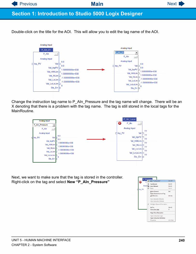
Previous Next



Double-click on the title for the AOI. This will allow you to edit the tag name of the AOI.

Change the instruction tag name to P_AIn_Pressure and the tag name will change. There will be an X denoting that there is a problem with the tag name. The tag is still stored in the local tags for the MainRoutine.

Next, we want to make sure that the tag is stored in the controller. Right-click on the tag and select New “P_AIn_Pressure”

Previous Next



The New Tag window will open. Click on Create to make a new tag under the Scope of My_Controls_Project. The new tag will be created as a Controller Tag, not a local MainRoutine tag. Storing tags in this manner will help the communication process between Studio 5000 programming and FactoryTalk View ME.

Double-Click on Controller Tags. You will see the new tag P_AIn_Laser in the list.

Previous Next


Next delete the local tag stored in the MainProgram > Parameters and Local Tags.


Click on the left square next to the tag that needs to be deleted. The whole tag will be highlighted in black. Right-click on the square and select Delete.

Go back to the SubRoutine window. Drag an input and output connection to the Analog Input page.

Previous Next



Wire the input and output of the P_AIn_Pressure FBD. Click on the nodes and select the desired location to wire the tag to.

Rename the output tag to Output_Pressure. Create a new tag in the scope of My_Controls_Project and select Create. The red X next to Output_Pressure will go away.

Next we need to wire the input to the proper channel on the 1734-IE2C. Recall that the pressure tranducer was connected to.

Previous Next



Wire the input and output of the P_AIn_Pressure FBD. Click on the nodes and select the desired location to wire the tag to. Locate the Local:2:I.Ch0Data tag and select it to connect the tag to the Inp_PV.

The red X error will go away and the P_AIn_Laser FBD is wired correctly.

Previous Next



Save My_Controls_Project by clicking the save button. Your new project should look like the diagram below:

1. How does a function block diagram simplify programming?

2. Describe how a function block diagram communicates tag data with a PAC.

3. Does the programmer need to know ladder logic to use the function block diagrams?

Section 1, Focus 4

Previous Next


Focus 5: Structured Text

Structured Text programming is another feature of the Logix Designer programming environment. It allows the programmer additional ways to accomplish a process task. Structured text can also be used to build custom AOIs that can be used on the FBD.

Next we can create a new AOI for the motor data. Right-click on Add-On Instructions to add a new instruction. Name the instruction P_Motor_Data. Be sure to select the Structured Text for the Type of instruction.


The new AOI definition window will pop up. Here we can add a description and enter the local tags that will be needed for the instructions.

Previous Next



Next, create the new tags for the AOI. Be sure to select the proper usage for the tag (Input vs Output) It is sometimes useful to label inputs and outputs directly in the tag. It can avoid confusion when writing the programming for the local tags.

• Current_In• Current_Out• Efficiency_Out• Horsepower_Out• Power_In• Power_In_Output• Power_Out_Output• RPM_In• RPM_Out• Torque_Out_Ftlb• Torque_Out_Nm• Voltage_In• Voltage_Out

In order to write the code for the P_Motor_Data structured text, we must first investigate some basic programming techniques. This form of programming can account for many different scenarios. This is universal (to some extent) to most programming languages. The main structured text statements in ControlsLabTM are:

IfThenElseElsifEnd_If

Previous Next



The main goal of the P_Motor_Data AOI is to create outputs for the types of motor data that the ControlsLabTM system monitors. This same task can be accomplished by many of the built in FBD instructions such as less than, greater than, and logic. However, structured text can put all of these variables into one FBD. This consolidates programming and saves the PAC memory space.

In programming, data is read from left to right, top to bottom (just like reading a book).The first structured text programming that needs to be written is the RPM Output code.

Open the structured text Logic window by double-clicking Logic in the P_Motor_Data AOI.

Write the following text in that window:(*RPM / Frequency Output*)

If the code is written correctly it will turn green. This code is strictly a means of labeling code within the structured text. It is not necessary for the program to operate, but allows the programmer to quickly navigate the code if any changes or problems occur. After placing the label, we can write the specific code below for the RPM / Frequency data:

If RPM_In > 0 ThenRPM_Out := RPM_In;

Frequency_Out := RPM_Out / 30;

Local tags in the structured text will automatically turn red. This lets the programmer know that an eligible tag has been selected for the specific task. Keep in mind, structured text programming also has a built in error checker similar to the other types of programming.

This code is simply checking to see IF RPM data is available (any number greater than 0) on RPM_In. Then, RPM_Out is defined to be equal to (:=) RPM_In. The semi-colon basically says that the specific part of the instruction is finished. This may seem redundant, but this is needed to show proper motor output. The frequency is the RPM divided by 30. We can use RPM_Out in the next line because the code from the previous line would be executed first.

Previous Next



Next we need to define when the output of RPM_Out and Frequency_Out is zero using the Else programming statement. In this case Else represents all other cases from above. Our next line of code is the following:

Else RPM_Out := 0;Frequency_Out := 0;

End_If;

Else RPM_Out is defined to be equal to zero. This means that all other cases for RPM_In will provide an RPM output of zero. With this code, the HMI can display a value of 0 when the motor is not running. If we didn’t have this code, the RPM_Out and Frequency_Out value would be empty or blank on the HMI control screen. The End_If code is there to mark the end of the If statement. The end must be marked so the processor knows when that code has been executed. It is like the period at the end of the sentence. It must be defined in order to move on to the next sentence.

The final RPM / Frequency programming statement should be the following:(*RPM Output*)If RPM_In > 0 Then RPM_Out := RPM_In; Frequency_Out := RPM_Out / 30;Else

RPM_Out := 0;Frequency_Out := 0;

End_If;

Next we can use similar arguments to define the motor data for voltage and current. Write the code as followes:

(*Voltage Current Output*)If Voltage_In > 0 Then

Voltage_Out := Voltage_In / 10;Current_Out := Current_In / 100;

ElseVoltage_Out := 0;Current_Out := 0;

End_If;

The data from the PowerFlex 525 is scaled (multiplied) at the output. The code above will be used to take that data in, and scale it back to its proper output units. When voltage is present, current is also present so we don’t need two different If statements. Structured text programming allows computation of basic mathematics on local tags. Voltage_In / 10 takes the input voltage and divides the number by 10. This gets the motor voltage data to display the voltage correctly in terms of Volts. Current_In / 100 takes the input current and divides the number by 100. This gets the motor current data to display the current in terms of Amps. Note: In this case the If and Else statement have more than 1 condition. Each condition needs to be ended with a semi-colon or the processor will get confused.

Previous Next



The next section of code is a little more complicated. It uses the same basic features, but more math is needed to calculate power, torque, and efficiency. Write the code below into My_Controls_Project.

(*Torque Power Output*)If Power_In > 0 Then

Torque_Out_Nm := (9.5488 * Power_In * 10 / RPM_In);Power_In_Output := (Current_In / 100) * (Voltage_In / 10);Power_Out_Output := Power_In * 10;Efficiency_Out := (Power_Out_Output / Power_In_Output)*100;

ElseTorque_Out_Nm := 0;Power_In_Output := 0;Power_Out_Output := 0;Efficiency_Out := 0;

End_IF;

In order to understand the mathematics, we must first investigate torque. Basically, torque measures the amount of force required to make an object rotate. The force causes the shaft to move a specific distance, so it is very similar to work. The torque equation is as follows:

In this case, the power output from the VFD would need to be in kW. The VFD outputs its power value in hecto watts hW. The value is scaled to output data with the best resolution. In order to get our values kW, the power needs to be multiplied by 10. That is why the equation has Power_In * 10. Therefore,

Torque_Out_Nm := (9.5488*Power_In * 10 / RPM_In)

We know from Unit 1 that Power = Current X Voltage. We can calculate the power that the motor uses by taking the current and voltage values that run the motor. The next line of code is using the power equation. Like before, we need to divide current by 100 and voltage by 10 because the VFD is actually scaling the output values. Therefore,

Power_In_Output := (Current_In / 100) * (Voltage_In / 10)

The other power values output from the VFD (Power_In) are the amount of power that the motor is creating. Since energy is lost in all mechanical processes, this value is less than the power required to drive the motor. Like before, we needed to multiply this by 10 because of the output scaling that the VFD requires.

τ = 9.5488 × POUTPUTRPM

Previous Next



Using the two power values, we can calculate the efficiency of the moter by using the following equation. Power_Out_Output is the useful power that we get from the motor and is considered power out in the equation. Power_In_Output is the amount of power required to run the motor. Efficiency can be calculated with the following equation:

In all other cases, we want these values to be zero, so the rest of the code will be the following:

ElseTorque_Out_Nm := 0;Power_In_Output := 0;Power_Out_Output := 0;Efficiency_Out := 0;

End_IF;

The last piece of structured text from this section is the horsepower of the system. In automation plants, many of the motors and components are rated in horsepower. It is sometimes beneficial to show the horsepower that you get from the motor. This is power that the motor is producing (Power_In_Output), and is different than the power required to run the motor (Power_Out_Output). We can use the horsepower equation to set up the code. Power must be in kW.

The structured text code would be the following:

(*Horsepower Output*)If Power_In > 0 Then

Horsepower_Out := 1.341 * Power_In * 10;Else

Horsepower_Out := 0;End_If;

The result is the amount of useful work that the system can use over time. Note: this is different from the 0.5 HP rating on the drive.

E = POUTPIN

×100%

HP = 1.341× P

Previous Next



The final structured text for the P_Motor_Data AOI is below:

Keep in mind, this is not the only way to accomplish the task of monitoring motor data. This is setup with structured text to show how mathematics and equations can easily be handled with this form of programming.

The next step in programming is to wire the P_Motor_Data AOI in the function block. Close the logic window for the AOI and open the function block diagram by clicking on the SubRoutine.

Previous Next



Right-click on the AOI and select Properties. P_Motor_Data Properties window will open.

Navigate to the add-on toolbar above the sheet. P_Motor_Data should now show up as a button. Click on the button and P_Motor_Data AOI will be added to the new function block diagram. The AOI will look like it is empty. We need to enable all of the inputs and outputs that were customized with structured text.

Open a new sheet in the function block diagram by clicking on the sheet image. Name the new sheet Motor Data.

Previous Next



Enable the desired items by clicking on the check boxes in the Vis column. Click OK to enable the items. Note: there is a column to the left showing I/O data. This may be useful for finding inputs or outputs quickly.

The AOI should now show the desired I/O data.

Previous Next


Rename the AOI Motor_Data and create a new tag Motor Data in the scope of My_Controls_Project. Delete P_Motor_Data_01 from MainProgram > Parameters and Local Tags.


Drag 9 output tags from the tool bar to the function block diagram. Name all of the output tags as shown below. Right-click on each tag and add a new output tag to the scope My_Controls_Project. This allows the PAC access to the data calculated from the AOI (since AOI data is local).

Previous Next


The finished AOI should look like the diagram below. It should also be free of errors. We are not going to add inputs at this time. Inputs will be added in Unit 6: VFD.


1. Explain why structured text can simplify and replace function block diagram mathematics.

2. Describe how structured text can be used in conjuction with a function block diagram.

3. Why is structured text is similar to other programming languages?

Section 1, Focus 4

Previous Next


Focus 6: I/O Tag Data

The L16ER controller uses communications to transmit I/O data. The communication format that you choose determines the data structure for the tags that are associated with the module. Many I/O modules support different formats. Each format uses a different data structure.


The controller uses different types of connections to transmit I/O data. These connections can be direct connections or rack-optimized connections. ControlsLabTM uses all direct connections in the communications network. Module connection types are visible in the properties window of the module. See the Parent section for the module. This will determine if the module is local or remote.

Previous Next



To add a new tag in studio 5000, right-click on the Controller Tags and select New Tag.

Choose the scope for the new tag. Choose the data type for the new tag. Choose external access for the new tag. Name the tag and select Create.

Previous Next


To add extended properties to a tag, open controller tags. At the bottom of the window there is a tab for “monitor tags” and “edit tags.” In this case we want to edit tags. Tags you can edit are shown in white. Tags that cannot be edited are shown in gray. Select a desired tag to change the extended properties. On the right side, there is a drop down


We are going to edit the extended properties of the tag Output_Efficiency. Select the boxes to add all three properties to the tag. Fields will show up below for the respective boxes. Enter the extended tag data in the boxes. The default values are automatically loaded. Efficiency is a percentage so set the min and max to 0 and 100 respectively. Set the Engineering Unit to %.

Previous Next


1.


____________________________________ _____________________________

Your Signature Date



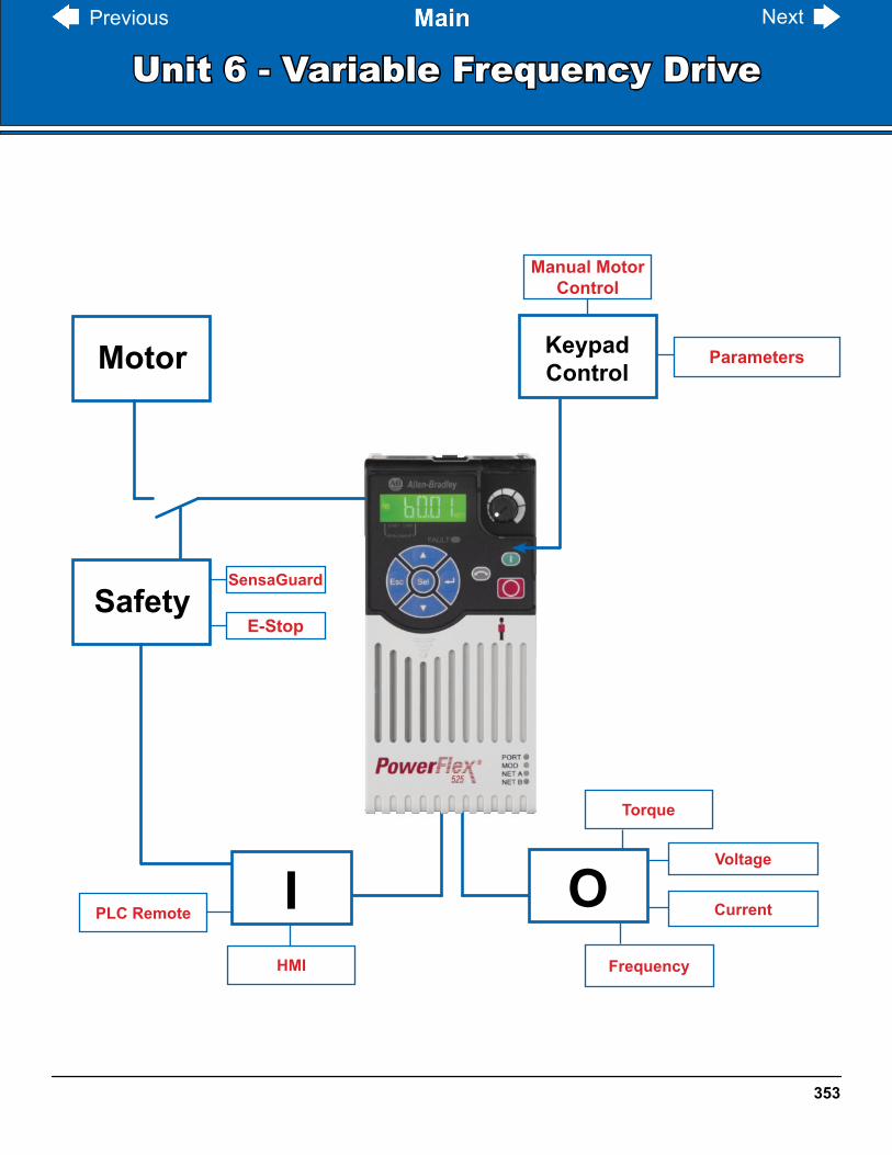
Previous Next

353

OVoltage

Torque

Frequency

CurrentIPLC Remote

HMI

KeypadControl

Parameters

Manual Motor Control

SafetyE-Stop

SensaGuard

Motor

Unit 6 - Variable Frequency Drive

Previous Next

354UNIT 6 - VARIABLE FREQUENCY DRIVECHAPTER 1 - Introduction to PowerFlex 525

Chapter 1 - Introduction to PowerFlex 525

Section 1 – Drive Setup• Drive Wiring• I/O Features

Section 2 – Drive Parameters• Parameter Basics• Ethernet Parameters

ControlsLabTM uses a variable frequency drive to control the motor on the centrifugal blower.

Previous Next


Focus 1: Drive Wiring

Section 1: Drive Setup

The main wiring for the PowerFlex 525 drive consists of 120V input, and 220V 3-phase output to the Leeson motor. The diagram below shows the basic wiring for the PowerFlex 525 drive.

120V Input

Previous Next


The drive has single and 3-phase inputs. ControlsLabTM uses a 220V single phase connection. 220V line 1 is connected to L1. 220V line 2 is connected to L2. T1 is connected to motor wires 1 and 7. T2 is connected to motor wires 2 and 8. T3 is connected to motor wires 3 and 9. Motor wires 4,5,and 6 are tied together for 3-phase low voltage. This wiring is also located on the nameplate of the Leeson motor. The ground wire from the motor is connected to one of the ground terminals on the drive.


S1 and S2 are jumpered to pin 3. This disables the safety input from the drive.

Previous Next


Focus 2: I/O Features


Previous Next


Focus 1: Parameter Basics

Section 2: Drive Parameters

Drive parameters can be setup with software, or manually from the drive. This focus will show you how to setup the Ethernet on the PowerFlex 525. Once connected to the network, it is easier to configure the other settings with software. We will explain those steps in the following pages.

The main display for the drive is shown below:

Previous Next



The diagram below shows the buttons on the keypad and explain their basic controls:

Previous Next



The steps below will show you how to navigate the keypad on the PowerFlex 525 drive. We will be using the keypad to set the network settings. This will allow the drive a connection to the control network. Once established, it is much easier to download the rest of the parameters via software.

Previous Next



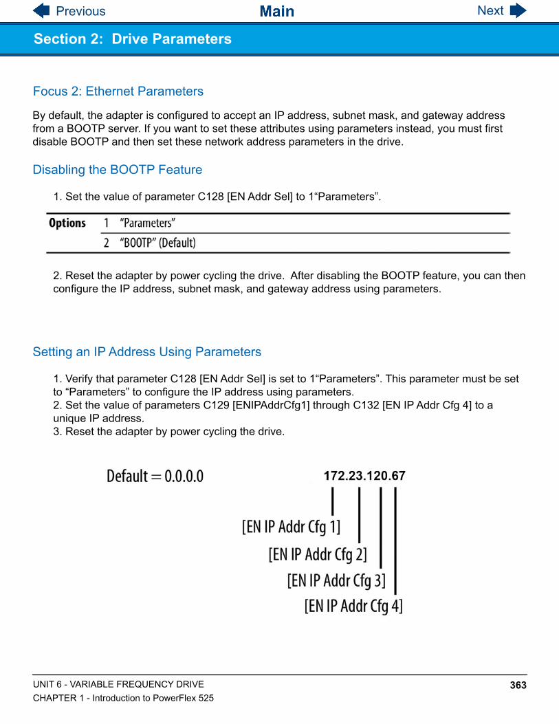
Previous Next


Focus 2: Ethernet Parameters


By default, the adapter is configured to accept an IP address, subnet mask, and gateway address from a BOOTP server. If you want to set these attributes using parameters instead, you must first disable BOOTP and then set these network address parameters in the drive.

Disabling the BOOTP Feature

1. Set the value of parameter C128 [EN Addr Sel] to 1“Parameters”.

2. Reset the adapter by power cycling the drive. After disabling the BOOTP feature, you can then configure the IP address, subnet mask, and gateway address using parameters.

Setting an IP Address Using Parameters

1. Verify that parameter C128 [EN Addr Sel] is set to 1“Parameters”. This parameter must be set to “Parameters” to configure the IP address using parameters.2. Set the value of parameters C129 [ENIPAddrCfg1] through C132 [EN IP Addr Cfg 4] to a unique IP address.3. Reset the adapter by power cycling the drive.

Previous Next



Setting a Subnet Mask Using Parameters

1. Verify that parameter C128 [ENENAddrSel] is set to 1 “Parameters”. This parameter must be set to “Parameters” to configure the subnet mask using parameters.2. Set the value of parameters C133 [ENSubnetCfg1] through C136 [EN Subnet Cfg 4] to the desired value for the subnet mask.3. Reset the adapter by power cycling the drive.

Setting a Gateway Address Using Parameters

1. Verify that parameter C128 [ENENAddrSel] is set to 1 “Parameters”. This parameter must be set to “Parameters” to configure the gateway address using parameters.2. Set the value of parameters C137 [ENGatewayCfg1] through C140 [EN Gateway Cfg 4] to the desired value for the gateway address.3. Reset the adapter by power cycling the drive.

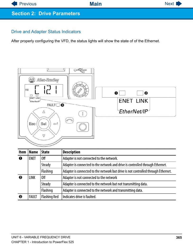
Previous Next



Drive and Adapter Status Indicators

After properly configuring the VFD, the status lights will show the state of of the Ethernet.

Previous Next


Chapter 2 - VFD Software Control

Section 1 – Basic Control• VFD Software Configuration• Studio 5000 Control Setup• FactoryTalk View ME Control Setup

Section 2 – PIDE Control• Studio 5000 PIDE Setup• FactoryTalk View ME PIDE Setup

ControlsLabTM uses software to manage and control the VFD. The software can handle basic drive operations, as well as advanced programming for PIDE control. The drive is connected via Ethernet, and is on the same control network as the HMI and PAC. This chapter will walk through the steps of drive configuration and setup for control using Studio 5000 Logix Designer and FactoryTalk View ME.

Previous Next


Focus 1: VFD Software Configuration

Section 1: Basic Control

Next we will setup the programming environment to run the PowerFlex 525 drive. Open My_Controls_Project in Studio 5000 Logix Designer. At the bottom of the controller organizer there should be a folder for I/O Configuration. Expand the folder so the subfolders are visible.

Right-click on the Ethernet device and select New Module.

A window will pop up to select a new module.

Previous Next



Search for PowerFlex 525.

Select the appropriate module and click Create.

Previous Next



A new window will pop up to configure the Module Properties. Type a name and description for the module. Define the IP Address of the module to be 172.23.120.67.

Navigate to the Port Configuration and set the Subnet Mask and Gateway Address to the properties previously configured for the device.

Previous Next



Select the Drive tab from Module Properties.

Select the Properties tab on the window.

Previous Next



The Properties window will pop up.

Select the Import/Export tab and click the Import button.

Previous Next



Navigate to C: > Turbine Technologies > ControlsLab Application Files and select the ControlsLab PF525 Parameters.iuux. Click Open. This will import the parameter configuration file for the ControlsLabTM system. If you wish to set each parameter individually, click cancel.

A new Import window will apear and gives two options. Select Import Entire Device and wait for the import to finish.

Previous Next



A window will appear stating any module differences. Click OK to accept thos differences.

Click Parameters to check the status of the import.

Previous Next



Scroll down to Parameter #46. It should now be set to EtherNetIP. The default setting for this parameter is Keypad. Therefore, the import was a sucess.

Go back to the General tab for Module properties. Click the button that says Change.

Previous Next


Click Apply to save the Module Properties. Click OK to exit the Module Properties window.

Change the Input Data to show the same values as the screen below. The data is output from the drive to the input of the PAC.


Previous Next



Now that the VFD is configured to output motor data to the PAC, we can wire the Motor Data sheet of the function block diagram. Open the Motor Data sheet from the SubRoutine in the MainRoutine.

Add four tag inputs to the P_Motor_Data function block diagram. Wire the inputs to the 4 input ports.

Previous Next



Locate the new tags that we previously setup for the VFD configuration. Navigate to Blower_PF525:I.OutputRPM.

Setup the rest of the VFD tags for P_Motor_Data. The finished FBD is shown below. This programming will be used for the Blowing display in FactoryTalk View ME.

ControlsLabTM - Turbine Technologies Sample.pdf · Focus 4 - PID Tuning ... Unit 8 - Studio 5000...

Documents

Transcript of ControlsLabTM - Turbine Technologies Sample.pdf · Focus 4 - PID Tuning ... Unit 8 - Studio 5000...