Controlling the onset of turbulence by streamwise travelling waves...

J. Fluid Mech. (2010), vol. 663, pp. 100–119. c© Cambridge University Press 2010

doi:10.1017/S002211201000340X

Controlling the onset of turbulenceby streamwise travelling waves.

Part 2. Direct numerical simulation

BINH K. LIEU, RASHAD MOARREFAND MIHAILO R. JOVANOVI C†

Department of Electrical and Computer Engineering, University of Minnesota,Minneapolis, MN 55455, USA

(Received 29 October 2009; revised 22 June 2010; accepted 23 June 2010;

first published online 8 September 2010)

This study builds on and confirms the theoretical findings of Part 1 of this paper(Moarref & Jovanovic, J. Fluid Mech., 2010, doi:10.1017/S0022112010003393). Weuse direct numerical simulation of the Navier–Stokes equations to assess the efficacyof blowing and suction in the form of streamwise travelling waves for controllingthe onset of turbulence in a channel flow. We highlight the effects of the modifiedbase flow on the dynamics of velocity fluctuations and net power balance. Oursimulations verify the theoretical predictions of Part 1 that the upstream travellingwaves promote turbulence even when the uncontrolled flow stays laminar. On theother hand, the downstream travelling waves with parameters selected in Part 1 arecapable of reducing the fluctuations’ kinetic energy, thereby maintaining the laminarflow. In flows driven by a fixed pressure gradient, a positive net efficiency as largeas 25 % relative to the uncontrolled turbulent flow can be achieved with downstreamwaves. Furthermore, we show that these waves can also relaminarize fully developedturbulent flows at low Reynolds numbers. We conclude that the theory developed inPart 1 for the linearized flow equations with uncertainty has considerable ability topredict full-scale phenomena.

Key words: flow control, transition to turbulence, turbulence control

1. IntroductionThe problem of controlling channel flows using strategies that do not require

measurement of the flow quantities and disturbances has recently received significantattention. Examples of these sensorless approaches to flow control include wall-geometry deformation such as riblets, transverse wall oscillations and control ofconductive fluids using the Lorentz force, to name only a few. Min et al. (2006) useddirect numerical simulation (DNS) to show that surface blowing and suction in theform of an upstream travelling wave (UTW) leads to a sustained sub-laminar drag ina fully developed turbulent channel flow. This motivated Marusic, Joseph & Mahesh(2007) to derive a criterion for achieving sub-laminar drag and to compare laminarand turbulent channel flows with and without control. Furthermore, Hœpffner &Fukagata (2009) characterized the mechanism behind UTWs as a pumping rather

† Email address for correspondence: [email protected]

Controlling the onset of turbulence by travelling waves: DNS study 101

than as a drag reduction; this is because the UTWs increase flux relative to theuncontrolled flow. Finally, Bewley (2009) and Fukagata, Sugiyama & Kasagi (2009)independently established that for any blowing and suction boundary actuation, thepower exerted at the walls is always larger than the power saved by reducing dragto sub-laminar levels. This led the authors of these two papers to conclude that theoptimal control solution is to relaminarize the flow.

Up to now, sensorless flow control strategies have been designed by combiningphysical intuition with extensive numerical and experimental studies. For example,a number of simulations on turbulent drag reduction by means of spanwise walloscillation were conducted by Quadrio & Ricco (2004), who considered 37 casesof different control parameters. Compared to the turbulent uncontrolled flow, amaximum drag reduction of 44.7 % was reported. However, analysis of the powerspent by the movement of the walls shows that a maximum net power gain of only7.3 % can be achieved. Even though DNS and experiments offer valuable insightinto sensorless strategies, their utility can be enhanced significantly by developing amodel-based framework for sensorless flow control design.

This paper builds directly on the theoretical findings of Part 1 (Moarref & Jovanovic2010), where receptivity analysis was used to show that the downstream travellingwaves (DTWs) are capable of reducing energy amplification of velocity fluctuationsin a transitional channel flow. The effectiveness of DTWs and UTWs in preventingor enhancing transition is examined in this study. In contrast to the current practice,we do not use DNS as a design tool; rather, we utilize it as a means for verificationand validation of theoretical predictions offered in Part 1 of this study. Namely,we use DNS to confirm that the DTWs with parameters selected in Part 1 cancontrol the onset of turbulence and achieve positive net efficiency relative to theuncontrolled flow that becomes turbulent. On the contrary, the UTWs enhancetransient growth and induce turbulence even when the uncontrolled flow stays laminar.In spite of promoting turbulence, the UTWs with large amplitudes can providesub-laminar drag coefficient. However, we show that this comes at the expense ofpoor net power balance in flows driven by a fixed pressure gradient. This is inagreement with Hœpffner & Fukagata (2009), who showed that it costs more toachieve the same amount of pumping using wall transpiration than the pressuregradient type of actuation. Our numerical simulations show the predictive power ofthe theoretical framework developed in Part 1 and suggest that the linearized Navier–Stokes (N–S) equations with uncertainty represent an effective control-oriented modelfor maintaining the laminar flow.

This paper is organized as follows. In § 2, we present the governing equations,describe the numerical method used in our simulations and outline the influenceof travelling waves on control net efficiency. The evolution of three-dimensionalfluctuations around base flows induced by surface blowing and suction is studied in § 3.We further emphasize how velocity fluctuations affect skin-friction drag coefficient andnet power balance. The energy-amplification mechanisms are discussed in § 3.4, wherewe show that the DTWs improve transient behaviour relative to the uncontrolledflow by reducing the production of kinetic energy. In addition, the effect of travellingwaves on coherent flow structures in transitional flows is visualized in § 3.5, where itis shown that the DTWs control the onset of turbulence by weakening the intensityof the streamwise streaks. In § 4, we show that the downstream waves designedin Part 1 can also relaminarize fully developed turbulent flows at low Reynoldsnumbers. We summarize our presentation and give a view of future research directionsin § 5.

102 B. K. Lieu, R. Moarref and M. R. Jovanovic

Flow

Downstream

y

x

z

Figure 1. A channel flow with blowing and suction along the walls.

2. Problem formulation and numerical method2.1. Governing equations

We consider a three-dimensional incompressible flow of a viscous Newtonian fluidin a straight channel (see figure 1 for geometry). The spatial coordinates (x, y, z) arescaled with the channel half-height, δ, and they denote the streamwise, wall-normaland spanwise directions, respectively; the velocities are scaled with the centrelinevelocity of the laminar parabolic profile, Uc; the pressure is scaled with ρU 2

c , whereρ denotes the fluid density; and the time is scaled with the convective time scale,δ/Uc. The flow is driven by a streamwise pressure gradient and it satisfies the non-dimensional N–S and continuity equations:

ut = − (u · ∇) u − ∇P + (1/Rc)u, 0 = ∇ · u. (2.1)

Here, Rc denotes the Reynolds number, Rc = Ucδ/ν, ν is the kinematic viscosity, uis the velocity vector, P is the pressure, ∇ is the gradient and is the Laplacian,= ∇ · ∇.

In addition to the constant pressure gradient, Px = −2/Rc, let the flow be subjectto a zero-net-mass-flux surface blowing and suction in the form of a streamwisetravelling wave (Min et al. 2006). The base velocity, ub =(U, V, W = 0), represents thesteady-state solution to (2.1) in the presence of the following boundary conditions:

V (y = ±1) = ∓2 α cos (ωx(x − c t)), U (±1) = Vy(±1) = W (±1) = 0, (2.2)

where ωx , c and α denote frequency, speed and amplitude of the streamwise travellingwave. Positive values of c identify a DTW, while negative values of c identify a UTW.In the presence of velocity fluctuations, u represents the sum of base velocity, ub, andvelocity fluctuations, v = (u, v, w), where u, v and w denote the fluctuations in thestreamwise, wall-normal and spanwise directions, respectively.

2.2. Numerical method

In this paper, the streamwise travelling waves, considered theoretically in Part 1, aretested in DNS of a three-dimensional transitional Poiseuille flow. All DNS calculationsare obtained using the code developed by Gibson (2007). A multistep semi-implicitAdams–Bashforth/backward-differentiation (AB/BDE) scheme described in Peyret(2002) is used for time discretization. The AB/BDE scheme treats the linear terms


Case Symbol c ωx α Lx/δ Lz/δ Ny Nx Nz

0 × − − − 2π 4π/3 65 50 501 5 2 0.035 2π 4π/3 65 50 502 5 2 0.050 2π 4π/3 65 50 503 5 2 0.125 2π 4π/3 65 50 504 −2 0.5 0.015 8π 4π/3 65 200 505 −2 0.5 0.050 8π 4π/3 65 200 506 −2 0.5 0.125 8π 4π/3 65 200 50

Table 1. The computational domain and spatial discretization considered in simulations ofthe uncontrolled flow, DTWs with (c = 5, ωx =2, α = 0.035, 0.050, 0.125) and UTWs with(c = −2, ωx = 0.5, α = 0.015, 0.050, 0.125). Symbols identify the corresponding flow in figuresthat follow. The box sizes in the streamwise and spanwise directions are denoted by Lx and Lz,respectively. The number of grid points in the streamwise, wall-normal and spanwise directionsare represented by Ni , i = x, y, z, respectively.

implicitly and the nonlinear terms explicitly. A spectral method (Canuto et al. 1988)is used for the spatial derivatives with Chebyshev polynomial expansion in thewall-normal direction and Fourier series expansion in the streamwise and spanwisedirections. Aliasing errors from the evaluation of the nonlinear terms are removed bythe 3/2-rule when the horizontal/Fourier transforms are computed. We modified thecode to account for the streamwise travelling wave boundary conditions (2.2).

The N–S equations are integrated in time with the objective of computingfluctuations’ kinetic energy, skin-friction drag coefficient and net power balance (see§ 3). The velocity field is first initialized with the laminar parabolic profile in theabsence of three-dimensional fluctuations (see § 2.3); this yields the two-dimensionalbase flow which is induced by the fixed pressure gradient, Px = −2/Rc, and theboundary conditions (2.2). In simulations of the full three-dimensional flows (cf. § 3),an initial three-dimensional perturbation is superimposed on the base velocity, ub.As the initial perturbation, we consider a random velocity field developed by Gibson(2007), which has the ability to trigger turbulence by exciting all the relevantFourier and Chebyshev modes. This divergence-free initial condition is composedof random spectral coefficients that decay exponentially and satisfy homogenousDirichlet boundary conditions at the walls. The flux and energy of the velocityfluctuations are computed at each time step.

A fixed pressure gradient is enforced in all simulations which are initiated atRc =2000; this value corresponds to the Reynolds number Rτ = 63.25 based on thefriction velocity uτ . Owing to the fixed pressure gradient, the steady-state value ofRτ is the same for all simulations, Rτ =63.25. In addition, we consider a streamwisebox length, Lx =4π/ωx , for all controlled flow simulations. This box length capturesthe streamwise modes kx = 0, ± ωx/2, ± ωx, ± 3ωx/2, . . .; relative to Part 1, thesemodes correspond to the union of the fundamental (kx = 0, ± ωx, ±2 ωx, . . .) andsubharmonic (kx = ± ωx/2, ± 3ωx/2, . . .) modes. In addition to the uncontrolledflow, we consider three DTWs with (c = 5, ωx =2, α = 0.035, 0.050, 0.125) andthree UTWs with (c = −2, ωx =0.5, α = 0.015, 0.050, 0.125). The complete list ofthe parameters along with the computational domain sizes and the number of spatialgrid points is shown in table 1. The total integration time is ttot = 1000 δ/Uc. We haveverified our simulations by making sure that the changes in results are negligible byincreasing the number of wall-normal grid points to Ny = 97.


Case c ωx α UB,N 103 Cf,N %Πprod %Πreq %Πnet

0 − − − 0.6667 4.5000 0 0 01 5 2 0.035 0.6428 4.8404 −3.58 16.64 −20.222 5 2 0.050 0.6215 5.1778 −6.77 31.74 −38.513 5 2 0.125 0.4821 8.6050 −27.69 136.50 −164.194 −2 0.5 0.015 0.6703 4.4513 2.70 5.46 −2.765 −2 0.5 0.050 0.7791 3.2949 16.86 37.69 −20.836 −2 0.5 0.125 1.0133 1.9478 51.99 145.05 −93.06

Table 2. Nominal results in a Poiseuille flow with Rτ = 63.25. The nominal flux, UB,N , andskin-friction drag coefficient, Cf,N , are computed using the base flow described in § 2.3.The produced power, %Πprod , the required power, %Πreq , and the net power, %Πnet , arenormalized by the power required to drive the uncontrolled flow. The produced and netpowers are computed with respect to the laminar uncontrolled flow.

1.0Downstream Upstream

(a)

0.5

0y

–0.5

–1.0

1.0(b)

0.5

0

–0.5

–1.00.4 0.6 0.8

α = 0.035

α = 0.015

α = 0.05

α = 0.125

α = 0.05

α = 0.125

No control

No control

1.00.20 0.4 0.6 0.8 1.0 1.20.20–0.2

Figure 2. Mean streamwise base velocity, U (y), obtained in two-dimensional simulations ofthe uncontrolled Poiseuille flow with Rτ = 63.25 (×), and controlled flows subject to: (a) DTWswith , (c = 5, ωx = 2, α = 0.035); , (c = 5, ωx =2, α = 0.05); , (c =5, ωx = 2, α = 0.125);and (b) UTWs with , (c = −2, ωx =0.5, α = 0.015); , (c = −2, ωx = 0.5, α = 0.05);, (c = −2, ωx = 0.5, α = 0.125).

2.3. Base flow and nominal net efficiency

Base velocity, ub = (U (x, y, t), V (x, y, t), 0), is computed using DNS of a two-dimensional Poiseuille flow with Rτ = 63.25 in the presence of a streamwise travellingwave boundary control (see (2.2)). Figure 2 shows the mean velocity profiles, U (y)(with overline denoting the average over horizontal directions), in an uncontrolledflow and in flows subject to selected DTWs and UTWs; these results agree with theresults obtained using Newton’s method in Part 1. The nominal bulk flux, whichquantifies the area under U (y),

UB,N =1

2

∫ 1

−1

U (y) dy, (2.3)

and the nominal skin-friction drag coefficient for three UTWs and three DTWs arereported in table 2. For the fixed pressure gradient, Px = −2/Rc, the nominal skin-friction drag coefficient is inversely proportional to the square of the nominal flux, i.e.

Cf,N = −2 Px/U2B,N . (2.4)


As shown by Hœpffner & Fukagata (2009), compared to the uncontrolled laminarflow, the nominal flux is reduced (increased) by DTWs (UTWs); according to (2.4),this results in larger (smaller) nominal drag coefficients, respectively.

The above results suggest that properly chosen travelling waves can exhibitincreased flux compared to the uncontrolled flow. For fixed pressure gradient, thisresults in production of a driving power,

Πprod = −Px(UB,c − UB,u)(2LxLz), (2.5)

where UB,c and UB,u denote the flux of the controlled and uncontrolled flows. Thenormalized produced power, %Πprod , is expressed as a percentage of the power spentto drive the uncontrolled flow, Πu = −PxUB,u(2LxLz),

%Πprod = 100(UB,c − UB,u)/UB,u. (2.6)

On the other hand, the input power required for maintaining the travelling waves isobtained from (Currie 2003)

Πreq =(

V P∣∣y=−1

− V P∣∣y=1

)LxLz, (2.7)

and the normalized required power, %Πreq , is expressed as

%Πreq = 100V P

∣∣y=−1

− V P∣∣y=1

−2 Px UB,u

. (2.8)

In order to assess the efficacy of travelling waves for controlling transitional flows,the control net power is defined as the difference between the produced and requiredpowers (Quadrio & Ricco 2004),

%Πnet = %Πprod − %Πreq , (2.9)

where %Πnet signifies how much net power is gained (positive %Πnet ) or lost (negative%Πnet ) in the controlled flow as a percentage of the power spent to drive theuncontrolled flow.

The nominal efficiency of the selected streamwise travelling waves in two-dimensional flows, i.e. in the absence of velocity fluctuations, is shown in table 2.Note that the nominal net power is negative for all controlled two-dimensionalsimulations. This is in agreement with a recent study of Hœpffner & Fukagata (2009),where it was shown that the net power required to drive a flow with wall transpirationis always larger than in the standard pressure gradient type of actuation.

3. Avoidance/promotion of turbulence by streamwise travelling wavesIn Part 1, it was shown that a positive net efficiency can be achieved in a situation

where the controlled flow stays laminar but the uncontrolled flow becomes turbulent.Whether the controlled flow can remain laminar depends on velocity fluctuationsaround the modified base flow. In this section, we study the influence of streamwisetravelling waves on the dynamics and the control net efficiency. This problem isaddressed by simulating a three-dimensional channel flow with initial perturbationswhich are superimposed on the base velocity induced by the wall actuation. Dependingon the kinetic energy of the initial condition, we distinguish three cases: (i) both theuncontrolled and properly designed controlled flows remain laminar (small initialenergy); (ii) the uncontrolled flow becomes turbulent, while the controlled flow stayslaminar for the appropriate choice of travelling-wave parameters (moderate initial


Initial energy Case (c) ωx α 103 Cf %Πprod %Πreq %Πnet

Small 0 − − − 4.5002 0 0 02 5 2 0.050 5.1778 −6.77 31.77 −38.544 −2 0.5 0.015 4.3204 −1.54 5.14 −3.605 −2 0.5 0.050 5.9426 −16.52 23.22 −39.746 −2 0.5 0.125 3.6853 12.20 108.41 −96.21

Moderate 0 − − − 10.3000 0 0 01 5 2 0.035 4.9244 52.07 26.44 25.632 5 2 0.050 5.2273 47.35 50.40 −3.054 −2 0.5 0.015 8.7866 11.36 4.53 6.835 −2 0.5 0.050 6.7406 31.15 41.96 −10.816 −2 0.5 0.125 3.9264 77.03 155.80 −78.77

Large 0 − − − 11.2000 0 0 02 5 2 0.050 11.9000 −3.37 47.90 −51.273 5 2 0.125 12.1000 −11.31 196.89 −208.205 −2 0.5 0.050 7.4438 13.68 34.19 −20.516 −2 0.5 0.125 3.9872 57.75 142.92 −85.17

Table 3. Results of three-dimensional simulations in a Poiseuille flow with Rτ = 63.25 forinitial conditions of small, moderate, and large energy (respectively, E(0) = 2.25 × 10−6,E(0) = 5.0625 × 10−4, and E(0) = 2.5 × 10−3). The values of Cf , %Πprod , %Πreq , and %Πnet

correspond to t = 1000. For small initial energy, the produced and net powers are computedwith respect to laminar uncontrolled flow; for moderate and large initial energies, they arecomputed with respect to turbulent uncontrolled flow.

energy); and (iii) both the uncontrolled and controlled flows become turbulent forselected travelling-wave parameters (large initial energy). Our simulations, however,indicate that poorly designed travelling waves can promote turbulence even for initialconditions for which the uncontrolled flow stays laminar. It was demonstrated in Part 1that properly designed DTWs are capable of significantly reducing the receptivity ofvelocity fluctuations, which makes them well suited for preventing transition; onthe other hand, compared to the uncontrolled flow, the velocity fluctuations aroundthe UTWs at best exhibit similar receptivity to background disturbances. FollowingPart 1, we present our main results for DTWs with (c = 5, ωx =2); these results arecompared to UTWs with (c = −2, ωx = 0.5) (as selected in Min et al. 2006). In bothcases, three wave amplitudes are selected (cf. table 1).

The three-dimensional simulations, which are summarized in table 3, confirm andcomplement the theoretical predictions of Part 1 at two levels. At the level ofcontrolling the onset of turbulence, we illustrate in § 3.1 that the UTWs increasethe receptivity of velocity fluctuations and promote turbulence even for initialperturbations for which the uncontrolled flow stays laminar. In contrast, the DTWscan prevent transition even in the presence of initial conditions with moderate andlarge energy (cf. §§ 3.2 and 3.3). At the level of net power efficiency, it is first shownin § 3.1 that the net power is negative when the uncontrolled flow stays laminar.However, for the uncontrolled flow that becomes turbulent, we demonstrate that theDTWs can result in a positive net efficiency. As discussed in §§ 3.2 and 3.3, the positivenet efficiency is achieved if the required power for maintaining the laminar DTW isless than the produced power. In addition, in § 3.3, we highlight an important trade-offthat limits the advantages of DTWs in controlling the onset of turbulence in flowssubject to large initial conditions. Namely, we show that, in this case, preventingtransition by DTWs requires a large input power that results in a negative efficiency.


2.5(×10–5)

1.5

0.5

Downstream(a)

0.10

0.06

0.02

0

Upstream(b)

α = 0.05

α = 0.05

α = 0.125

α = 0.015

No control

0 200 400t

600 800 1000 200 400t

600 800 1000

Figure 3. Energy of the velocity fluctuations, E(t), for the initial condition with small energy:(a) ×, uncontrolled; , a DTW with (c = 5, ωx = 2, α = 0.05); and (b) UTWs with , (c = −2,ωx = 0.5, α = 0.015); , (c = −2, ωx = 0.5, α = 0.05); , (c = −2, ωx = 0.5, α = 0.125).

Our simulations in § 3.2 reveal that although UTWs become turbulent, a positivenet efficiency can be achieved for sufficiently small wave amplitudes. For the initialconditions with moderate energy, we further point out that the achievable positivenet efficiency for UTWs is much smaller than for the DTWs that sustain the laminarflow (cf. § 3.2).

3.1. Small initial energy

We first consider the initial perturbations with small kinetic energy, E(0) = 2.25×10−6,which cannot trigger turbulence in a flow with no control. Our simulations show thatthe DTWs selected in Part 1 of this study improve transient response of the velocityfluctuations; on the contrary, the UTWs considered in Min et al. (2006) lead todeterioration of the transient response and, consequently, promote turbulence. Sincethe uncontrolled flow stays laminar, both DTWs and UTWs lead to the negative netefficiency.

The energy of velocity fluctuations is given by

E(t) =1

Ω

∫Ω

(u2 + v2 + w2) dΩ, (3.1)

where Ω = 2LxLz is the volume of the computational box. Figure 3 shows thefluctuations’ kinetic energy as a function of time for the uncontrolled flow andcontrolled flows subject to a DTW with (c = 5, ωx = 2, α =0.05) and three UTWswith (c = −2, ωx = 0.5, α = 0.015, 0.05, 0.125). As is evident from figure 3(a), theenergy of the uncontrolled flow exhibits a transient growth followed by an exponentialdecay to zero (i.e. to the laminar flow). We see that a DTW moves the transientresponse peak to a smaller time, which is about half the time at which the peak ofE(t) in the uncontrolled flow takes place. Furthermore, maximal transient growthof the uncontrolled flow is reduced by approximately 2.5 times, and a much fasterdisappearance of the velocity fluctuations is achieved. On the other hand, figure 3(b)clearly exhibits the negative influence of the UTWs on a transient response. Inparticular, the two UTWs with larger amplitudes significantly increase the energy ofvelocity fluctuations. We note that the fluctuations’ kinetic energy in a flow subject to aUTW with an amplitude as small as α = 0.015 at t = 1000 is already about two ordersof magnitude larger than the maximal transient growth of the flow with no control.


0 200 400

Cf %Πreq

%Πnet%Πprod

600 800 1000 0 200 400 600 800 1000

0 200 400t

600 800 1000 0 200 400t

600 800 1000

6

5

4

3

2

(a)

60

40

20

0

–20

(c)

50

20

–50

–100

(d)

150

100

50

0

(b)DTW, α = 0.05

(×10–3)

UTW, α = 0.125

UTW, α = 0.125

UTW, α = 0.05

DTW, α = 0.05

DTW, α = 0.05

UTW, α = 0.05

UTW, α = 0.125

UTW, α = 0.125

DTW, α = 0.05

UTW, α = 0.05

UTW, α = 0.05

No control

Figure 4. (a) Skin-friction drag coefficient, Cf ; (b) normalized required power, %Πreq ; (c)normalized produced power, %Πprod ; and (d ) normalized net power, %Πnet , for the initialcondition with small energy: ×, uncontrolled flow; , DTW with (c = 5, ωx =2, α = 0.05);and UTWs with , (c = −2, ωx = 0.5, α = 0.015); , (c = −2, ωx = 0.5, α = 0.05); , (c = −2,ωx = 0.5, α = 0.125).

Figure 4(a) shows the skin-friction drag coefficient,

Cf (t) =2τw

U 2B

=1

Rc U 2B

[(dU

dy+

du

dy

)∣∣∣∣y=−1

−(

dU

dy+

du

dy

)∣∣∣∣y=1

], (3.2)

as a function of time for the travelling waves considered in figure 3. Here, τw denotesthe non-dimensional average wall-shear stress and

UB(t) =1

2

∫ 1

−1

(U (y) + u(y, t)) dy (3.3)

is the total bulk flux. Since both the uncontrolled flow and the flow subject to aDTW stay laminar, their steady-state drag coefficients agree with the nominal valuescomputed in the absence of velocity fluctuations (cf. tables 2 and 3). On the otherhand, the drag coefficients of the UTWs that become turbulent are about twicethe values predicted using the base-flow analysis. The large amplification of velocityfluctuations by UTWs is responsible for this increase. The velocity fluctuations in theUTW with α = 0.015 are not sufficiently amplified to have a pronounced effect onthe drag coefficient. Furthermore, the drag coefficients for the UTWs with (c = −2,


ωx =0.5, α = 0.05, 0.125) at t = 1000 agree with the results of Min et al. (2006)computed for the fully developed turbulent channel flow. This indicates that theUTWs with larger amplitudes in our simulations have transitioned to turbulence.The above results confirm the theoretical prediction of Part 1, where it is shown thatthe UTWs are poor candidates for controlling the onset of turbulence for they increasereceptivity relative to the uncontrolled flow.

The normalized required, produced and net powers for the initial conditions withsmall kinetic energy are shown in figures 4(b)–4(d ). Note that the normalized netpower for all travelling waves is negative (cf. figure 4d ). This confirms the predictionof Part 1 that the net power is negative whenever the uncontrolled flow stays laminar.It is noteworthy that the UTW with α = 0.125 has a negative net power despite itssignificantly smaller drag coefficient compared to the laminar uncontrolled flow. Asevident from figures 4(b) and 4(c), this is because the required power for maintainingthis UTW is much larger than the power produced by reducing drag. The aboveresults agree with the studies of Bewley (2009) and Fukagata et al. (2009), where itwas established that the net cost to drive a flow by any transpiration-based strategyis larger than in the uncontrolled laminar flow. Therefore, aiming for a sub-laminardrag may not be advantageous from the efficiency point of view. Instead, one candesign control strategies that yield a smaller drag than the uncontrolled turbulentflow and provide positive net power balance (cf. § 3.2).

3.2. Moderate initial energy

We next consider the velocity fluctuations with moderate initial energy, E(0) = 5.0625×10−4. This selection illustrates a situation where the initial conditions are large enoughto trigger turbulence in the uncontrolled flow but small enough to allow the properlychosen DTWs to maintain the laminar flow and achieve positive net power balance.As shown in § 3.1, the UTWs trigger turbulence even for the initial conditions whosekinetic energy is about 200 times smaller than the value considered here.

The energy of the velocity fluctuations and drag coefficients as a function of timefor the uncontrolled flow and UTWs are shown in figures 5(a) and 5(b). Figure 5(a)indicates that the kinetic energy of the uncontrolled flow and the flow subject to UTWswith (c = −2, ωx =0.5, α = 0.015, 0.05, 0.125) is increased by orders of magnitude,which eventually results in transition to turbulence. This large energy amplificationof UTWs is captured by the linear analysis around the laminar base flows in Part 1.As is evident from figure 5(b), the large fluctuations’ energy in both the uncontrolledflow and UTWs yields much larger drag coefficients compared to the nominal valuesreported in table 2. In addition, figure 5(b) is in agreement with Min et al. (2006),where it was shown that the skin-friction drag coefficients of the UTWs are smallerthan in the uncontrolled flow that becomes turbulent, and that the UTW with(c = −2, ωx = 0.5, α = 0.125) achieves a sub-laminar drag. The normalized requiredand net powers for the UTWs are shown in figures 5(c) and 5(d ). Note that therequired power for maintaining the UTW with α = 0.125 (which yields a sub-laminardrag) is so large that it results in a negative net power balance (cf. figure 5d ). Onthe other hand, the UTW with α = 0.015 is capable of producing a small positive netpower for two main reasons: (i) it has a smaller drag coefficient than the uncontrolledturbulent flow (although it becomes turbulent itself) and (ii) it requires a much smallerpower compared to the UTW with α =0.125.

The fluctuations’ kinetic energy and skin-friction drag coefficient for the DTWsare shown in figures 6(a) and 6(b). Figure 6(a) shows that the DTWs with(c = 5, ωx = 2, α = 0.035, 0.05) significantly weaken intensity of the velocity


0.1010

8

6

4

2

0.06

0.02

0 200 400 600 800 1000

0 200 400 600 800 1000 0 200 400 600 800 1000

0 200 400 600 800 1000

(a)

250

150

50

0

–50

–100

–150

50

–50

(c)

(b)

(d)

α = 0.125

α = 0.05α = 0.015

α = 0.015

α = 0.125

α = 0.05

α = 0.015

α = 0.125

α = 0.05

No control

No control

Laminar

t t

(×10–3)E Cf

%Πreq %Πnet

α = 0.015

α = 0.05

α = 0.125

Figure 5. (a) Energy of the velocity fluctuations, E(t); (b) skin-friction drag coefficient,Cf (t); (c) normalized required power, %Πreq ; and (d ) normalized net power, %Πnet ,for the initial condition with moderate energy: ×, uncontrolled; and UTWs with, (c = −2, ωx = 0.5, α = 0.015); , (c = −2, ωx = 0.5, α =0.05); , (c = −2, ωx = 0.5, α = 0.125).

fluctuations, thereby facilitating maintenance of the laminar flow. From figure 6(b)we also see that the small transient growth of fluctuations’ kinetic energy results ina small transient increase in the drag coefficients which eventually decay to theirnominal values reported in table 2. Even though these drag coefficients are largerthan in the uncontrolled laminar flow, they are still approximately twice as small asin the uncontrolled flow that becomes turbulent (cf. table 3).

The normalized produced, required and net powers for DTWs are shown infigures 6(c) and 6(d ). As can be seen from figure 6(c), the normalized producedpower for the DTWs is positive by virtue of the fact that the uncontrolled flowbecomes turbulent while the controlled flows stay laminar. Figure 6(d ) showsthat the DTW with α = 0.035 (respectively, α = 0.05) has a positive (respectively,negative) net power balance. The reason for this is twofold: first, as is evident fromfigure 6(c), the DTW with larger α results in a smaller produced power since itinduces a larger negative nominal bulk flux than the DTW with smaller α; andsecond, the required power to maintain the DTW with larger α is greater thanthat needed for the DTW with smaller α. Furthermore, at t = 1000, the DTW withα = 0.035 has a larger net power than the UTW with α = 0.015 (%Πnet = 25.63 versus%Πnet = 6.83; cf. table 3). This is because the DTW with α = 0.035, in contrast to


3

2

1

60

40

20

0

–20

0

(a)

(c)20

0

–20

–40

–60

(d)

5.4(b)

5.2

5.0

4.8

0 200 400 600 800 1000

200 400 600 800 1000 0 200 400 600 800 1000

t0 200 400 600 800 1000

t

α = 0.035

α = 0.05

α = 0.05

α = 0.035

α = 0.035

α = 0.035

α = 0.05

α = 0.05

(×10–3) (×10–3)E Cf

%Πreq, %Πprod %Πnet

Figure 6. (a) Energy of the velocity fluctuations, E(t); (b) skin-friction drag coefficient, Cf (t);(c) normalized required power, %Πreq (solid line), normalized produced power, %Πprod (dashedline); and (d ) normalized net power, %Πnet , for the initial condition with moderate energy:DTWs with , (c =5, ωx = 2, α = 0.035); , (c = 5, ωx = 2, α = 0.05).

the UTW with α =0.015, remains laminar and produces a much larger power than itrequires.

In summary, the results of this section highlight an important trade-off that needsto be taken into account when designing the travelling waves. Large amplitudesof properly designed downstream waves yield larger receptivity reduction, which isdesirable for controlling the onset of turbulence. However, this is accompanied byan increase in drag coefficient and required control power. Thus, to maximize netefficiency, it is advantageous to select the smallest possible amplitude of wall actuationthat can maintain the laminar flow.

3.3. Large initial energy

Section 3.2 illustrates the capability of properly designed DTWs to maintain thelaminar flow in the presence of initial conditions that induce transition in theuncontrolled flow. In this section, we demonstrate that, as the energy of the initialperturbation increases, a DTW with larger amplitude is needed to prevent transition.Our results confirm the prediction made in Part 1 that maintaining a laminar flowwith a larger DTW amplitude comes at the expense of introducing a negative netpower balance.


0.10

0.06

0.02

(a)

250

150

50

0

–50

–200

–100

0

–300

(c) (d)

0.015

0.010

0.005

(b)

0 200 400 600 800 1000

0 200 400 600 800 1000

t0 200 400 600 800 1000

0 200 400 600 800 1000

t

α = 0.125

α = 0.125α = 0.05

α = 0.05

α = 0.05

α = 0.05

α = 0.125

α = 0.125No control

No control

E Cf

%Πreq, %Πprod %Πnet

Figure 7. (a) Energy of the velocity fluctuations, E(t); (b) skin-friction drag coefficient,Cf (t); (c) normalized required power, %Πreq (solid line), normalized produced power, %Πprod

(dashed line); and (d ) normalized net power, %Πnet , for the initial condition with largeenergy: ×, uncontrolled; DTWs with , (c = 5, ωx =2, α = 0.05) and DTWs with , (c = 5,ωx = 2, α = 0.125).

Simulations in this section are done for the initial condition with large kineticenergy, E(0) = 2.5 × 10−3. The time evolution of the fluctuations’ energy for a pair ofDTWs with (c =5, ωx = 2, α = 0.05, 0.125) is shown in figure 7(a). The uncontrolledflow becomes turbulent and exhibits similar trends in the evolution of E(t) asthe corresponding flow initiated with moderate energy perturbations (cf. figures 5aand 7a). On the other hand, figure 7(a) shows that the DTW with α = 0.05 is notcapable of maintaining the laminar flow; in comparison, the same set of controlparameters prevented transition for the perturbations of moderate initial energy(cf. figures 6a and 7a). Conversely, the DTW with α = 0.125 remains laminar eventhough E(t) transiently reaches about half the energy of the turbulent uncontrolledflow. Therefore, the DTWs with frequency and speed selected in Part 1 and sufficientlylarge amplitudes are capable of maintaining the laminar flow even in the presence oflarge initial perturbations.

Figure 7(b) shows the skin-friction drag coefficients for the flows considered infigure 7(a). For the DTW with α =0.05, the steady-state value of Cf is given byCf =11.9 × 10−3, which is a slightly larger value than in the turbulent uncontrolledflow, Cf = 11.2 × 10−3 (cf. table 3). We note that the drag coefficient of the DTWthat stays laminar initially reaches values that are about 50 % larger than in the


uncontrolled flow; after this initial increase, Cf (t) then gradually decays to the valuepredicted using the base-flow analysis, Cf = 8.6 × 10−3 (cf. table 2). Figures 7(c)and 7(d ) show the normalized required, produced and net powers for the initialcondition with large kinetic energy. As is evident from figure 7(d ), the net powerbalance is negative for all considered flows. The DTW with α = 0.05 becomesturbulent, and it has a larger drag coefficient than the uncontrolled flow, whichconsequently leads to negative produced and net powers. Moreover, even thoughthe DTW with α = 0.125 can sustain the laminar flow, its net power balance is verypoor. There are two main reasons for the lack of efficiency of this control strategy:first, its nominal drag coefficient is significantly larger than in a DTW with smalleramplitudes, which consequently yields very small produced power (at larger times notshown in figure 7c); and second, a prohibitively large power is required to maintainthis large-amplitude DTW.

The results of this section show that preventing transition by DTWs in the presenceof large initial conditions comes at the expense of large negative net power balance.We also highlight that in the presence of large initial perturbations (or, equivalently,at large Reynolds numbers), transition to turbulence may be inevitable. Furthermore,the results of § 3.2 show that the UTWs may reduce the turbulent skin-friction dragand achieve positive net efficiency. The approach used in Part 1 considers dynamicsof fluctuations around laminar flows and, thus, it cannot be used for explaining thepositive efficiency of the UTWs that become turbulent.

3.4. Energy-amplification mechanisms

The Reynolds–Orr equation can be used to quantify the evolution of fluctuations’kinetic energy around a given base flow (Schmid & Henningson 2001). In this section,we use this equation to examine mechanisms that contribute to production anddissipation of kinetic energy in flows subject to travelling waves. For base velocity,ub = (U (x, y, t), V (x, y, t), 0), the evolution of the energy of velocity fluctuations, E(t),is determined by

1

2

dE

dt= PE(t) + DE(t),

PE(t) = − 1

Ω

∫Ω

(uvUy + uvVx + v2Vy + u2Ux) dΩ,

DE(t) =1

RcΩ

∫Ω

v · v dΩ.

⎫⎪⎪⎪⎪⎪⎪⎬⎪⎪⎪⎪⎪⎪⎭

(3.4)

Here, PE represents the production of kinetic energy and is associated with the work ofthe Reynolds stresses on the base shear, whereas DE accounts for viscous dissipation.

We confine our attention to the simulations for initial conditions with small energy.This situation is convenient for explaining why the DTWs exhibit improved transientbehaviour compared to the laminar uncontrolled flow while the UTWs promotetransition to turbulence. Figure 8(a) shows production and dissipation terms for theuncontrolled flow and for the flow subject to a DTW with (c = 5, ωx = 2, α = 0.05).For the uncontrolled flow, PE is always positive, DE is always negative and they bothdecay to zero at large times. On the contrary, the production term for the DTWbecomes negative for 80 t 220. We see that, at early times, PE and DE for theDTW follow their uncontrolled flow counterparts. However, after this initial period,they decay more rapidly to zero. These results confirm the prediction of Part 1 that theDTWs reduce the production of kinetic energy. In contrast, figure 8(b) shows that the


2

Production

Dissipation

Production

Dissipation

1

0

–1

Downstream: PE, DE Upstream: PE, DE(a) 0.4

0.2

0

–0.2

(b)

0 200 400t

600 800 1000 0 200 400t

600 800 1000

Upstream: PE + DE

0.10

0.05

0

–0.05

(c)

0 200 400t

600 800 1000

(×10–5)

Figure 8. (a) and (b) Production, PE(t) (solid line), and dissipation, DE(t) (dashed line), ofkinetic energy in a Poiseuille flow with Rτ = 63.25 for the initial condition with small energy:(a) ×, uncontrolled; , DTW with (c = 5, ωx =2, α = 0.05); and (b) , UTW with (c = −2,ωx = 0.5, α = 0.05); , UTW with α =0.125. (c) PE(t) + DE(t) for the UTW with (c = −2,ωx = 0.5, α = 0.05).

UTWs with (c = −2, ωx = 0.5, α = 0.05, 0.125) increase both PE and DE by aboutfour orders of magnitude compared to the values reported in figure 8(a). This verifiesthe theoretical prediction of Part 1 that the UTWs increase the production of kineticenergy. Moreover, production dominates dissipation transiently, thereby inducing thelarge growth of kinetic energy observed in figure 3(b). For the UTW with α =0.05,this is further illustrated in figure 8(c) by showing that PE accumulates more energythan DE dissipates (i.e. the area under the curve in figure 8c is positive). We also notethat, in the above simulations, the work of Reynolds stress uv on the base shear Uy

dominates the other energy production terms. Furthermore, our results show that thewall-normal diffusion of u is responsible for the largest viscous energy dissipation.

3.5. Flow visualization

In §§ 3.1–3.3, transition was identified by examining fluctuations’ kinetic energy andskin-friction drag coefficients. Large levels of sustained kinetic energy and substantialincrease in drag coefficients (compared to base flows) were used as indicators oftransition. Here, we use flow visualization to identify coherent structures in both theuncontrolled and controlled flows.


4

3

2z

1

0 2 4 6

0.10

0.05

0

–0.05

–0.10

(a) 4

3

2

1

0 2 4 6

0.10

0.05

0

–0.05

–0.10

(c)4

3

2

1

0 10 20

0.2

0.1

0

–0.1

–0.2

(b)

4

3

2z

1

0 2x x x

4 6

0.1

0.2

0

–0.1

(d) 4

3

2

1

0 2 4 6

0.05

0

–0.05

( f )4

3

2

1

0 10 20

0.1

0

–0.1–0.2–0.3

(e)

Uncontrolled:t = 50

Upstream:t = 50

Downstream:t = 50

t = 120 t = 120 t = 120

Figure 9. Streamwise velocity fluctuations, u(x, z), at y = −0.5557 (y+ = 28.11), (a)–(c) t = 50,and (d )–(f ) t = 120 for initial condition with moderate energy: uncontrolled flow; UTW with(c = −2, ωx =0.5, α =0.05); and DTW with (c = 5, ωx = 2, α = 0.05).

The onset of turbulence in a bypass transition is usually characterized by theformation of streamwise streaks and their subsequent breakdown. For the initialcondition with moderate energy, figure 9 shows the streamwise velocity fluctuationsat y = −0.5557 (y+ =28.11 in wall units) for the uncontrolled flow and flows subjectto a UTW with (c = −2, ωx =0.5, α = 0.05) and a DTW with (c = 5, ωx = 2, α = 0.05).Clearly, the initial perturbations evolve into streamwise streaks in all three flows (cf.figures 9a–9c for t =50). At t = 120, the growth of velocity fluctuations results in abreakdown of the streaks both in the flow with no control and in the flow subjectto UTWs (cf. figures 9d and 9e). We see that the streaks evolve into complex flowpatterns much more rapidly in the latter case. For the UTWs, the streak distortionoccurs as early as t = 50 and a broad range of spatial scales is observed at t =120. Onthe contrary, figure 9(f ) shows that, at t =120, the DTWs have reduced the magnitudeof velocity fluctuations to about half the value at t = 50, thereby weakening intensityof the streaks and maintaining the laminar flow.

4. Relaminarization by downstream wavesThus far, we have shown that properly designed DTWs represent an effective means

for controlling the onset of turbulence. In this section, we demonstrate that the DTWsdesigned in Part 1 can also relaminarize fully developed turbulent flows. Since thelifetime of turbulence depends on the Reynolds number (Brosa 1989; Grossmann2000; Hof et al. 2006; Borrero-Echeverry, Schatz & Tagg 2010), we examine turbulentflows with Rc = 2000 (i.e. Rτ ≈ 63.25) and Rc =4300 (i.e. Rτ ≈ 92.80).

The numerical scheme described in § 2.2 is used to simulate the turbulent flows. ForRc =4300, the number of grid points in the streamwise, wall-normal and spanwisedirections is increased to 80 × 97 × 80. The velocity field is initialized with a fullydeveloped turbulent flow obtained in the absence of control. The surface blowing andsuction that generates DTWs is then introduced (at t = 0), and the kinetic energy anddrag coefficients are computed at each time step.


500 1000 1500 2000

0.12

0.08

0.04

0

α = 0.035

No control

α = 0.125

α = 0.05

t

Figure 10. Energy of velocity fluctuations around base flows of § 2.1. Simulations areinitiated by a fully developed turbulent flow with Rc = 2000: ×, uncontrolled; DTWs with, (c = 5, ωx = 2, α = 0.035); , (c = 5, ωx = 2, α = 0.05); and , (c = 5, ωx = 2, α = 0.125).

0.20

0.15

0.10

0.05

(a)

0.020

0.015

0.010

0.005

(b)

0 500 1000 1500 2000 2500t

0 500 1000 1500 2000 2500t

α = 0.035α = 0.035

No control

No controlα = 0.05

α = 0.05

α = 0.125 α = 0.125

E Cf

Figure 11. (a) Energy of velocity fluctuations around base flows of § 2.1, E(t); and(b) skin-friction drag coefficient, Cf (t). Simulations are initiated by a fully developedturbulent flow with Rc = 4300: ×, uncontrolled; DTWs with , (c = 5, ωx = 2, α = 0.035);, (c =5, ωx = 2, α = 0.05); and , (c = 5, ωx = 2, α = 0.125).

The fluctuations’ kinetic energy for the uncontrolled flow and for the flows subjectto DTWs with (c = 5, ωx = 2, α = 0.035, 0.05, 0.125) at Rc = 2000 are shown infigure 10. The energy of velocity fluctuations around base flows ub of § 2.1 (parabolafor a flow with no control; travelling waves for a flow with control) are shown;relaminarization occurs when the energy of velocity fluctuations converges to zero.Clearly, large levels of fluctuations in the flow with no control are maintained upuntil t ≈ 1100. After this time instant, however, velocity fluctuations exhibit gradualdecay. On the other hand, fluctuations in flows subject to DTWs start decaying muchearlier, thereby indicating that the lifetime of turbulence is reduced by surface blowingand suction. Relative to the uncontrolled flow, the fluctuations’ kinetic energy for theDTWs considered here converge much more rapidly to zero. We also see that the rateof decay increases as the wave amplitude gets larger.

We next consider a turbulent flow with Rc = 4300. The energy of velocity fluctuationsaround base flows ub of § 2.1 is shown in figure 11(a). In both the uncontrolledflow and the flows subject to the DTWs with (c = 5, ωx = 2, α = 0.035, 0.05),


1.0

0.5 4

3

2

1

0 2 4 6

0y

z

z

x

x

x

–0.5

–1.00–0.2 0.2

t = 0

t = 100

t = 900

0.4 0.62 4 6

4

3

2

1

0

z

4

3

2

1

0

2 4 6

0.8

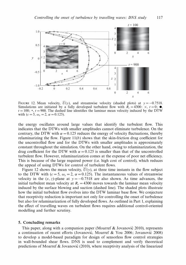
Figure 12. Mean velocity, U (y), and streamwise velocity (shaded plots) at y = −0.7518.Simulations are initiated by a fully developed turbulent flow with Rc = 4300: ×, t =0; ,t =100; ∗, t = 900. The dashed line identifies the laminar mean velocity induced by the DTWwith (c = 5, ωx = 2, α = 0.125).

the energy oscillates around large values that identify the turbulent flow. Thisindicates that the DTWs with smaller amplitudes cannot eliminate turbulence. On thecontrary, the DTW with α =0.125 reduces the energy of velocity fluctuations, therebyrelaminarizing the flow. Figure 11(b) shows that the skin-friction drag coefficient forthe uncontrolled flow and for the DTWs with smaller amplitudes is approximatelyconstant throughout the simulation. On the other hand, owing to relaminarization, thedrag coefficient for the DTW with α = 0.125 is smaller than that of the uncontrolledturbulent flow. However, relaminarization comes at the expense of poor net efficiency.This is because of the large required power (i.e. high cost of control), which reducesthe appeal of using DTWs for control of turbulent flows.

Figure 12 shows the mean velocity, U (y), at three time instants in the flow subjectto the DTW with (c = 5, ωx = 2, α = 0.125). The instantaneous values of streamwisevelocity in the (x, z)-plane at y = −0.7518 are also shown. As time advances, theinitial turbulent mean velocity at Rc = 4300 moves towards the laminar mean velocityinduced by the surface blowing and suction (dashed line). The shaded plots illustratehow the initial turbulent flow evolves into the DTW laminar base flow. We conjecturethat receptivity reduction is important not only for controlling the onset of turbulencebut also for relaminarization of fully developed flows. As outlined in Part 1, explainingthe effect of travelling waves on turbulent flows requires additional control-orientedmodelling and further scrutiny.

5. Concluding remarksThis paper, along with a companion paper (Moarref & Jovanovic 2010), represents

a continuation of recent efforts (Jovanovic, Moarref & You 2006; Jovanovic 2008)to develop a model-based paradigm for design of sensorless flow control strategiesin wall-bounded shear flows. DNS is used to complement and verify theoreticalpredictions of Moarref & Jovanovic (2010), where receptivity analysis of the linearized


N–S equations was used to design small-amplitude travelling waves. We haveshown that perturbation analysis (in the wave amplitude) represents a powerfulsimulation-free method for predicting full-scale phenomena and controlling the onsetof turbulence.

Simulations of nonlinear flow dynamics have demonstrated that the DTWs,designed in Part 1, can maintain a laminar flow and achieve positive net efficiency.In contrast, the UTWs promote turbulence even with the initial conditions for whichthe uncontrolled flow remains laminar. Our analysis of the Reynolds–Orr equationshows that, compared to the uncontrolled flow, the DTWs (UTWs) reduce (increase)the production of kinetic energy.

We have also examined the effects of DTWs on fully developed turbulent flows atlow Reynolds numbers. It turns out that the DTWs with speed and frequency selectedin Part 1 and sufficiently large amplitudes can eliminate turbulence (i.e. relaminarizethe flow). We also note that, in spite of promoting turbulence, the UTWs may stillachieve smaller drag coefficients compared to the uncontrolled flow. By increasingthe UTW amplitude, even a sub-laminar drag can be attained (Min et al. 2006). Itis, however, to be noted that large wave amplitudes introduce poor net efficiency inflows subject to a fixed pressure gradient. Nevertheless, these travelling waves maystill be utilized when the primal interest is to eliminate turbulence (with DTWs) orreduce the skin-friction drag (with UTWs) irrespective of the cost of control.

All simulations in this study are enforced by a fixed pressure gradient, as opposed tothe constant-mass-flux simulations of Min et al. (2006). This is consistent with Part 1where receptivity analysis was done for flows driven by a fixed pressure gradient.Even though these set-ups are equivalent in steady flows (Scotti & Piomelli 2001),they can exhibit fundamentally different behaviour in unsteady flows. For example, thetwo simulations may possess different stability characteristics and yield structurallydifferent solutions for near-wall turbulence (Waleffe 2001; Jimenez et al. 2005).Moreover, Jimenez et al. (2005) remarked that the dynamical properties of the twosimulations can significantly differ in small computational domains. Also, Kerswell(2005) suggested that specifying the simulation type comes next to defining theboundary conditions.

In order to examine the effect of simulation type on transition, skin-friction dragcoefficient and control net efficiency, we have repeated some of the simulations byadjusting the pressure gradient to maintain a constant mass flux. Our results revealthat regardless of the simulation type, the DTWs designed in Part 1 are effectivein preventing transition while the UTWs promote turbulence. Moreover, the steady-state skin-friction drag coefficients are almost identical in both cases. However,the control net efficiency significantly depends on the type of simulation. This isbecause of the difference in the definition of the produced power: in the fixed-pressure-gradient set-up, the produced power is captured by the difference betweenthe bulk fluxes in the uncontrolled and controlled flows; in the constant-mass-fluxset-up, the produced power is determined by the difference between the drivingpressure gradients in the uncontrolled and controlled flows. It turns out that theproduced power is larger in the constant-mass-flux simulation than in the fixed-pressure-gradient simulation, whereas the required power remains almost unchanged.Consequently, both DTWs and UTWs have larger efficiency in constant-mass-fluxsimulations. For example, in the fixed-pressure-gradient set-up of the present study,the UTWs with (c = −2, ωx =0.05, α = 0.05, 0.125) have negative efficiency. Theefficiency of these UTWs is, however, positive in constant-mass-flux simulations (Minet al. 2006). Our ongoing effort is directed towards understanding the reason behind


this disagreement which may be ultimately related to the fundamental differencebetween these two types of simulations.

Financial support from the National Science Foundation under CAREER AwardCMMI-06-44793 and 3M Science and Technology Fellowship (to R.M.) is gratefullyacknowledged. The authors also thank Dr J. Gibson for helpful discussions regardingthe Channelflow code. The University of Minnesota Supercomputing Institute isacknowledged for providing computing resources.

REFERENCES

Bewley, T. R. 2009 A fundamental limit on the balance of power in a transpiration-controlledchannel flow. J. Fluid Mech. 632, 443–446.

Borrero-Echeverry, D., Schatz, M. F. & Tagg, R. 2010 Transient turbulence in Taylor–Couetteflow. Phys. Rev. E 81 (2), 25301.

Brosa, U. 1989 Turbulence without strange attractor. J. Stat. Phys. 55 (5), 1303–1312.

Canuto, C., Hussaini, M. Y., Quarteroni, A. & Zang, T. A. 1988 Spectral Methods in FluidDynamics . Springer.

Currie, I. G. 2003 Fundamental Mechanics of Fluids . CRC Press.

Fukagata, K., Sugiyama, K. & Kasagi, N. 2009 On the lower bound of net driving power incontrolled duct flows. Physica D: Nonlinear Phenom. 238 (13), 1082–1086.

Gibson, J. F. 2007 Channelflow: a spectral Navier–Stokes solver in C++. Tech. Rep., GeorgiaInstitute of Technology, www.channelflow.org.

Grossmann, S. 2000 The onset of shear flow turbulence. Rev. Mod. Phys. 72, 603–618.

Hœpffner, J. & Fukagata, K. 2009 Pumping or drag reduction? J. Fluid Mech. 635, 171–187.

Hof, B., Westerweel, J., Schneider, T. M. & Eckhardt, B. 2006 Finite lifetime of turbulence inshear flows. Nature 443 (7), 59–62.

Jimenez, J., Kawahara, G., Simens, M. P., Nagata, M. & Shiba, M. 2005 Characterization ofnear-wall turbulence in terms of equilibrium and ‘bursting’ solutions. Phys. Fluids 17 (1),015105.

Jovanovic, M. R. 2008 Turbulence suppression in channel flows by small amplitude transverse walloscillations. Phys. Fluids 20 (1), 014101.

Jovanovic, M. R., Moarref, R. & You, D. 2006 Turbulence suppression in channel flows by meansof a streamwise traveling wave. In Proceedings of the 2006 Summer Program , pp. 481–494.Center for Turbulence Research, Stanford University/NASA.

Kerswell, R. R. 2005 Recent progress in understanding the transition to turbulence in a pipe.Nonlinearity 18, R17–R44.

Marusic, I., Joseph, D. D. & Mahesh, K. 2007 Laminar and turbulent comparisons for channelflow and flow control. J. Fluid Mech. 570, 467–477.

Min, T., Kang, S. M., Speyer, J. L. & Kim, J. 2006 Sustained sub-laminar drag in a fully developedchannel flow. J. Fluid Mech. 558, 309–318.

Moarref, R. & Jovanovic, M. R. 2010 Controlling the onset of turbulence by streamwise travellingwaves. Part 1. Receptivity analysis. J. Fluid Mech. 663, 70–99.

Peyret, R. 2002 Spectral Methods for Incompressible Viscous Flow . Springer.

Quadrio, M. & Ricco, P. 2004 Critical assessment of turbulent drag reduction through spanwisewall oscillations. J. Fluid Mech. 521, 251–271.

Schmid, P. J. & Henningson, D. S. 2001 Stability and Transition in Shear Flows . Springer.

Scotti, A. & Piomelli, U. 2001 Numerical simulation of pulsating turbulent channel flow. Phys.Fluids 13 (5), 1367–1384.

Waleffe, F. 2001 Exact coherent structures in channel flow. J. Fluid Mech. 435, 93–102.

Controlling the onset of turbulence by streamwise travelling waves...

Documents

Transcript of Controlling the onset of turbulence by streamwise travelling waves...