Controlling theFalse Discovery Rate: From Astrophysics to

Bioinformatics

Jim LinnemannMSU Physics

Bioinformatics SeminarNovember 5, 2003

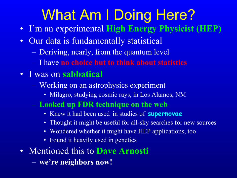
What Am I Doing Here?• I’m an experimental High Energy Physicist (HEP)• Our data is fundamentally statistical

– Deriving, nearly, from the quantum level– I have no choice but to think about statistics

• I was on sabbatical– Working on an astrophysics experiment

• Milagro, studying cosmic rays, in Los Alamos, NM– Looked up FDR technique on the web

• Knew it had been used in studies of supernovae• Thought it might be useful for all-sky searches for new sources• Wondered whether it might have HEP applications, too• Found it heavily used in genetics

• Mentioned this to Dave Arnosti– we’re neighbors now!

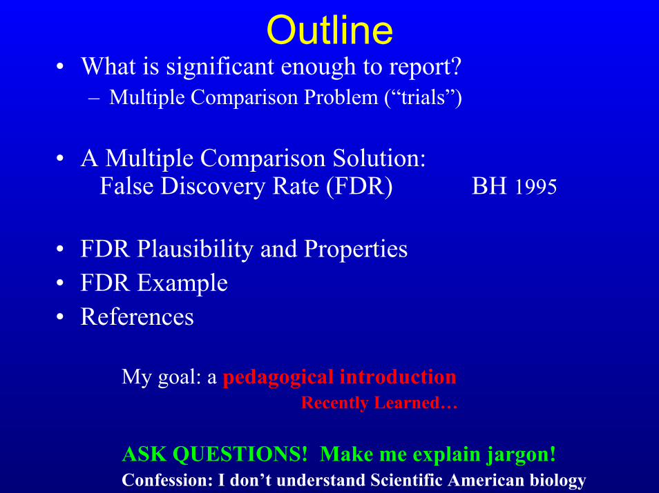
Outline• What is significant enough to report?

– Multiple Comparison Problem (“trials”)

• A Multiple Comparison Solution:False Discovery Rate (FDR) BH 1995

• FDR Plausibility and Properties• FDR Example• References

My goal: a pedagogical introductionRecently Learned…

ASK QUESTIONS! Make me explain jargon!Confession: I don’t understand Scientific American biology

Thanks to:• Slides from web:

– T. Nichol Umich (also for colorful slide template) – C. Genovese CMU– Y. Benjamini Tel Aviv, S. Scheid, MPI

• Email advice and pointers to literature– C. Miller CMU Astrophysics– B. Efron Stanford, J. Rice Berkeley ,

Y. Benjamani Tel Aviv Statistics– Google “False Discovery Rate”

– Had pleasure of meeting Genovese, Efron, RiceAt PHYSTAT 2003 conference (Astronomy, Physics, Statistics)

The Problem:• I: You have a really good idea. You find a

positive effect at the .05 significance level.

• II: While you are in Stockholm, your students work very hard. They follow up on 100 of your ideas, but have somehow misinterpreted your brilliant notes. Still, they report 5 of them gave significant results. Do you book a return flight?

Significance• Define “wrong” as reporting false positive:

– Apparent signal caused by background

• Set α a level of potential wrongness– 2 σ =.05 3 σ = .003 etc.

• Probability of going wrong on one test• Or, error rate per test

– “Per Comparison Error Rate” (PCER)• Statisticians say: “z value” instead of z σ’s

– Or “t value”

What if you do m tests?• Search m places• Must be able to define “interesting”

– e.g. “not background”• Examples from HEP and Astrophysics

• Look at m histograms, or bins, for a bump• Look for events in m decay channels• Test standard model with m measurements (not just Rb or g-2)• Look at m phase space regions for a Sleuth search (Knuteson)

• Fit data to m models: What’s a bad fit?• Reject bad tracks from m candidates from a fitting routine• Look for sources among m image pixels• Look for “bursts” of signals during m time periods• Which of m fit coefficients are nonzero?

– Which (variables, correlations) are worth including in the model?– Which of m systematic effect tests are significant?

Rather than testing each independently

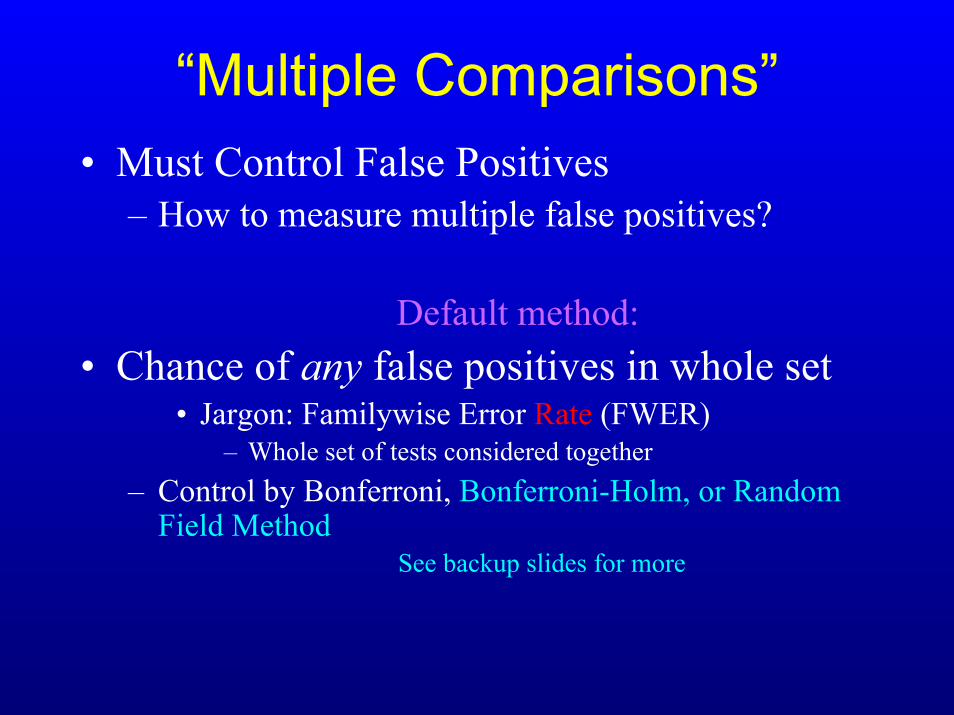
“Multiple Comparisons”• Must Control False Positives

– How to measure multiple false positives?

Default method:• Chance of any false positives in whole set

• Jargon: Familywise Error Rate (FWER)– Whole set of tests considered together

– Control by Bonferroni, Bonferroni-Holm, or Random Field Method

See backup slides for more

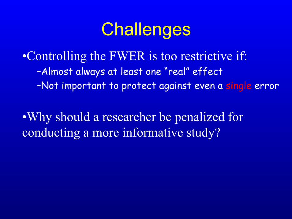
Challenges•Controlling the FWER is too restrictive if:

–Almost always at least one “real” effect–Not important to protect against even a single error

•Why should a researcher be penalized for conducting a more informative study?

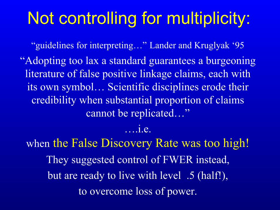
Not controlling for multiplicity:“guidelines for interpreting…” Lander and Kruglyak ‘95

“Adopting too lax a standard guarantees a burgeoning literature of false positive linkage claims, each with its own symbol… Scientific disciplines erode their credibility when substantial proportion of claims

cannot be replicated…” ….i.e.

when the False Discovery Rate was too high!They suggested control of FWER instead, but are ready to live with level .5 (half!),

to overcome loss of power.

Must do something about m!– m is “trials factor” only NE Jour Med demands!– Don’t want to just report m times as many signals

• P(at least one wrong) = 1 – (1- α)m ~ mα

– Use α/m as significance test “Bonferroni correction”• This is the main method of control

– Keeps to α the probability of reporting 1 or more wrong on whole ensemble of m tests

– Good: control publishing rubbish– Bad: lower sensitivity (must have more obvious signal)

• For some purposes, have we given up too much?

Bonferroni Who?• "Good Heavens! For more than forty years

I have been speaking prose without knowing it."-Monsieur Jourdan in

"Le Bourgeoise Gentilhomme" by Moliere

False Discovery Rate (FDR)

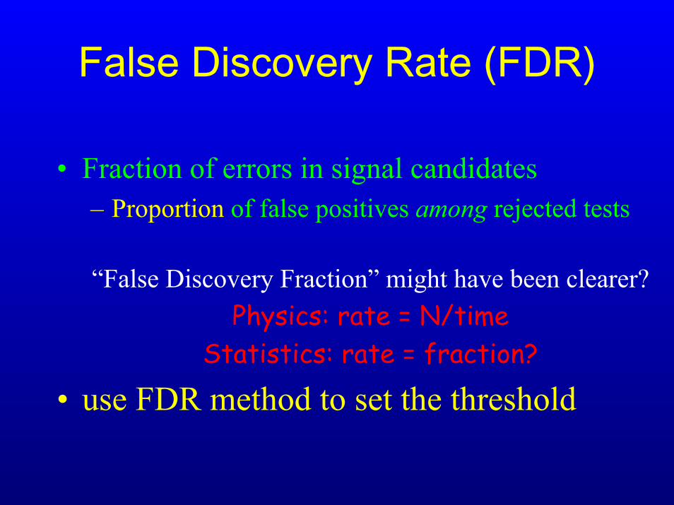
• Fraction of errors in signal candidates– Proportion of false positives among rejected tests

“False Discovery Fraction” might have been clearer?Physics: rate = N/time

Statistics: rate = fraction?

• use FDR method to set the threshold

Historical perspectiveTukey, when expressing support for the use of FDR, points back to his own (1953) as the roots of the idea!(?) He clearly was

looking over these years for some approach in between the too soft PCE and the too

harsh FWE.

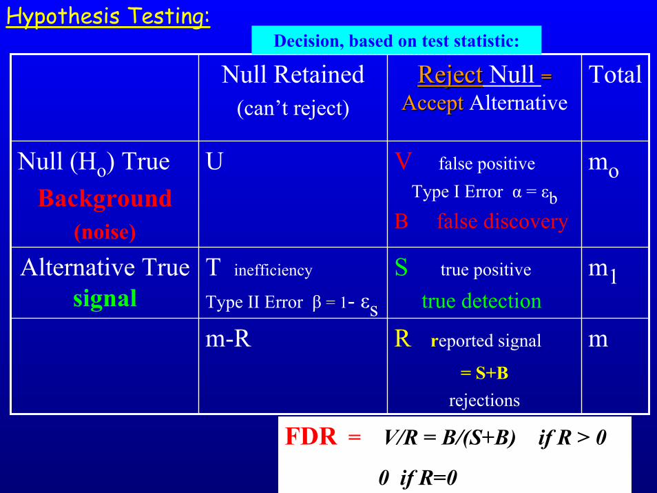
Hypothesis Testing:

mR reported signal

= S+Brejections

m-R

m1S true positive

true detectionT inefficiency

Type II Error β = 1- εs

Alternative True signal

moV false positiveType I Error α = εb

B false discovery

UNull (Ho) TrueBackground

(noise)

TotalRejectReject Null ==AcceptAccept Alternative

Null Retained(can’t reject)

Decision, based on test statistic:

FDR = V/R = B/(S+B) if R > 0

0 if R=0

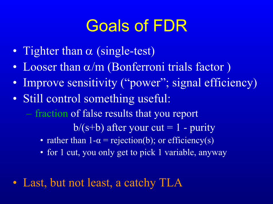
Goals of FDR• Tighter than α (single-test)• Looser than α/m (Bonferroni trials factor )• Improve sensitivity (“power”; signal efficiency)• Still control something useful:

– fraction of false results that you reportb/(s+b) after your cut = 1 - purity

• rather than 1-α = rejection(b); or efficiency(s)• for 1 cut, you only get to pick 1 variable, anyway

• Last, but not least, a catchy TLA

Where did this come from?Others who have lots of tests!

• Screening of chemicals, drugs• Genetic mapping

“Whereof one cannot speak, one must remain silent” --Wittgenstein• Functional MRI (voxels on during speech processing)• Data mining: which claimed relationships are real?

– Display cookies by the milk? Best of all market basket item-item associations– Direct mail strategy? Fit to: $ last time; time since last contribution…

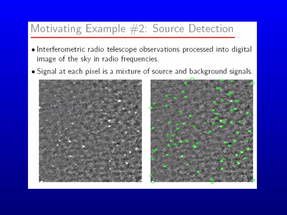
• Radio telescope images (at last some astronomy!)

Common factors:– One false positive does not invalidate overall conclusion– Usually expect some real effects– Can follow up by other means

• Trigger next phase with mostly real stuff

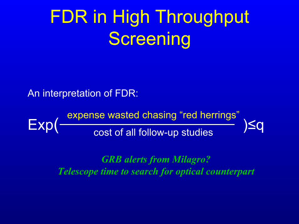
FDR in High Throughput Screening

An interpretation of FDR:

expense wasted chasing “red herrings”

cost of all follow-up studiesExp( )≤q

GRB alerts from Milagro?Telescope time to search for optical counterpart

FDR in a nutshell

– Search for non-background events– Need only the background probability distribution– Control fraction of false positives reported

• Automatically select how hard to cut, based on that

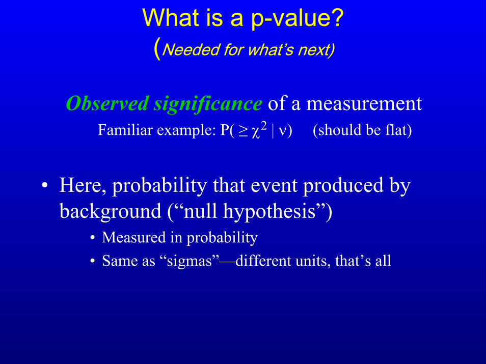
What is a p-value?(Needed for what’s next)

Observed significance of a measurementFamiliar example: P( ≥ χ2 | ν) (should be flat)

• Here, probability that event produced by background (“null hypothesis”)

• Measured in probability• Same as “sigmas”—different units, that’s all

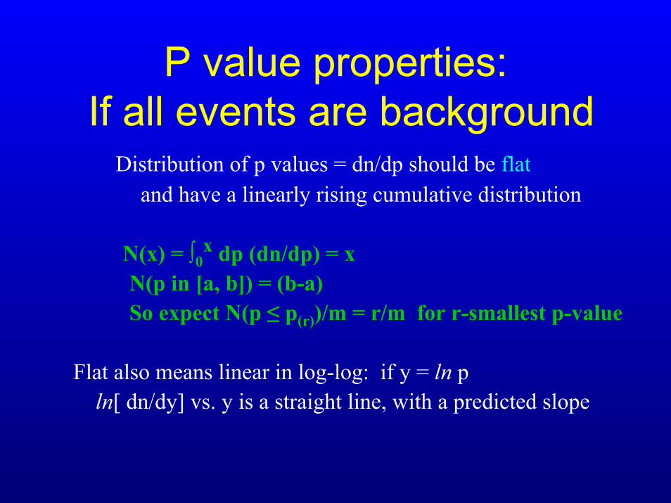
P value properties:If all events are background

Distribution of p values = dn/dp should be flatand have a linearly rising cumulative distribution

N(x) = ∫0x dp (dn/dp) = x

N(p in [a, b]) = (b-a) So expect N(p ≤ p(r))/m = r/m for r-smallest p-value

Flat also means linear in log-log: if y = ln pln[ dn/dy] vs. y is a straight line, with a predicted slope

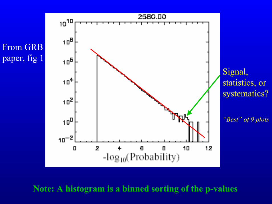
From GRB paper, fig 1

Signal, statistics, or systematics?

“Best” of 9 plots

Note: A histogram is a binned sorting of the p-values

Benjamini & Hochberg

• Select desired limit q on Expectation(FDR) α is not specified: the method selects it

• Sort the p-values, p(1) ≤ p(2) ≤ ... ≤ p(m)• Let r be largest i such that

For now, take c(m)=1

• Reject all null hypotheses corresponding top(1), ... , p(r).– i.e. Accept as signalAccept as signal

• Proof this works is not obvious!

p(i)

i/m

q(i/m)/c(m)p-

valu

e

0 1

01

q ~ .15

JRSS-B (1995) 57:289-300

p(i) ≤ q(i/m)/c(m)

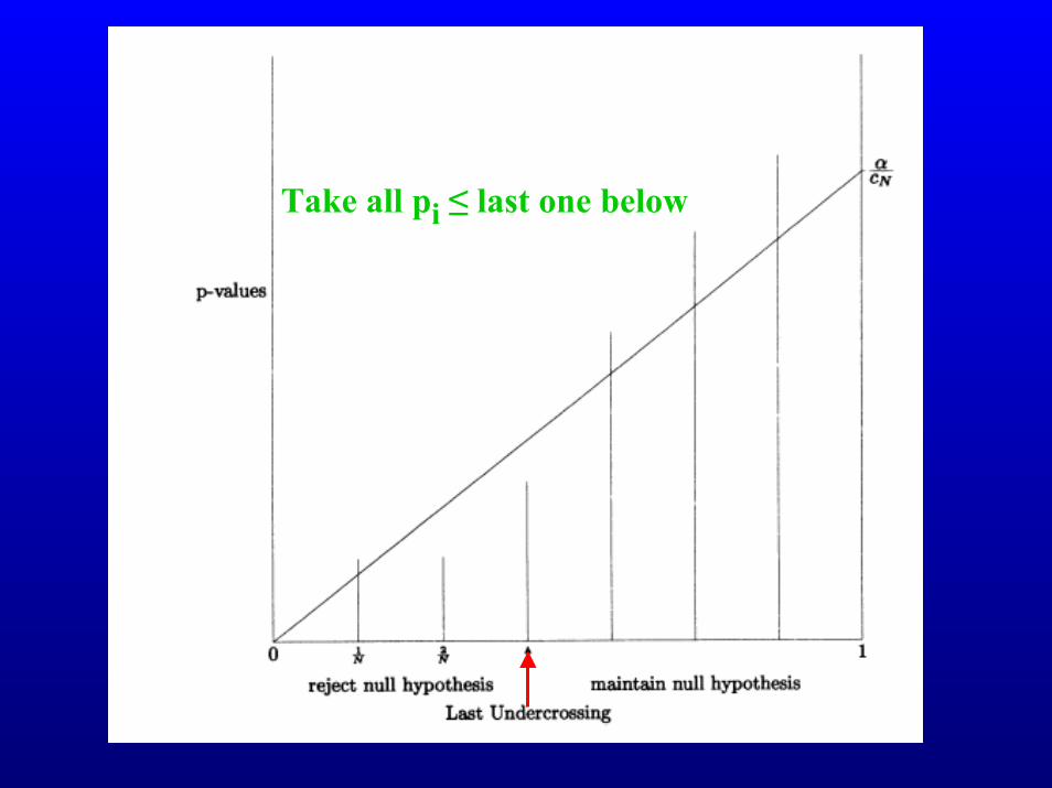
Take all pi ≤ last one below

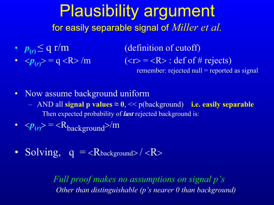
Plausibility argumentfor easily separable signal of Miller et al.

• p(r) ≤ q r/m (definition of cutoff)• <p(r)> = q <R> /m (<r> = <R> : def of # rejects)

remember: rejected null = reported as signal

• Now assume background uniform– AND all signal p values ≈ 0, << p(background) i.e. easily separable

Then expected probability of last rejected background is:

• <p(r)> = <Rbackground>/m

• Solving, q = <Rbackground> / <R>

Full proof makes no assumptions on signal p’sOther than distinguishable (p’s nearer 0 than background)

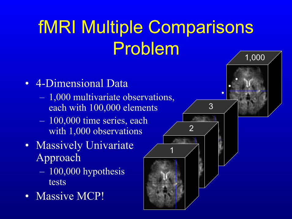
fMRI Multiple Comparisons Problem

• 4-Dimensional Data– 1,000 multivariate observations,

each with 100,000 elements– 100,000 time series, each

with 1,000 observations• Massively Univariate

Approach– 100,000 hypothesis

tests• Massive MCP!

1,000

1

2

3

. . .

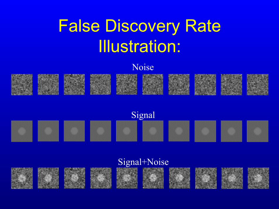
False Discovery RateIllustration:

Noise

Signal

Signal+Noise

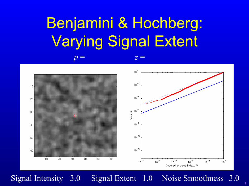
Benjamini & Hochberg:Varying Signal Extent

p = z =

Signal Intensity 3.0 Signal Extent 1.0 Noise Smoothness 3.01

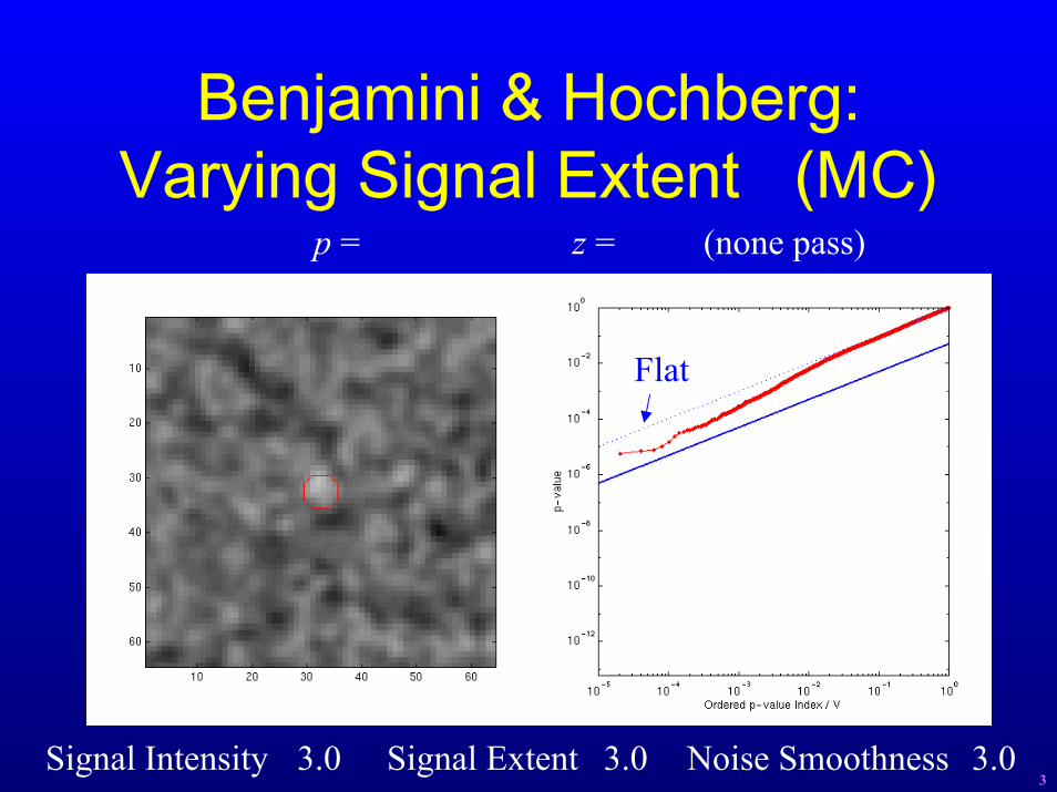
Benjamini & Hochberg:Varying Signal Extent (MC)

p = z = (none pass)

Flat

Signal Intensity 3.0 Signal Extent 3.0 Noise Smoothness 3.03

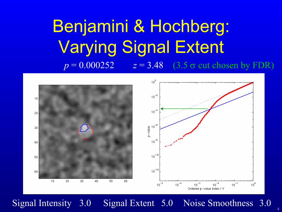
Benjamini & Hochberg:Varying Signal Extent

p = 0.000252 z = 3.48 (3.5 σ cut chosen by FDR)

Signal Intensity 3.0 Signal Extent 5.0 Noise Smoothness 3.04

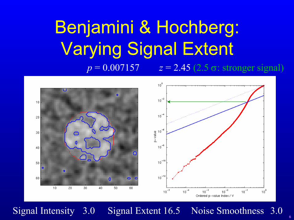
Benjamini & Hochberg:Varying Signal Extent

p = 0.007157 z = 2.45 (2.5 σ: stronger signal)

Signal Intensity 3.0 Signal Extent 16.5 Noise Smoothness 3.06

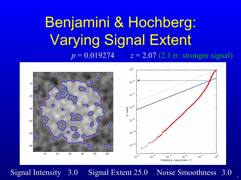
Benjamini & Hochberg:Varying Signal Extent

p = 0.019274 z = 2.07 (2.1 σ: stronger signal)

Signal Intensity 3.0 Signal Extent 25.0 Noise Smoothness 3.07

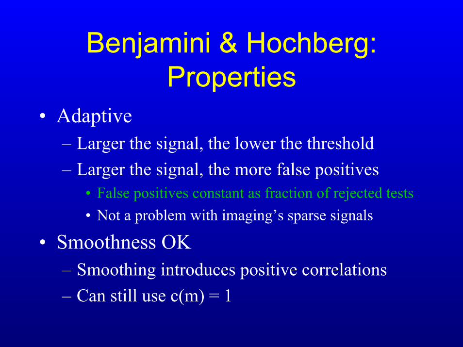
Benjamini & Hochberg: Properties

• Adaptive– Larger the signal, the lower the threshold– Larger the signal, the more false positives

• False positives constant as fraction of rejected tests• Not a problem with imaging’s sparse signals

• Smoothness OK– Smoothing introduces positive correlations– Can still use c(m) = 1

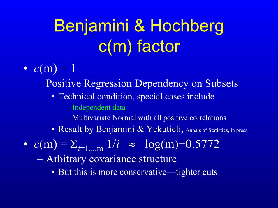
Benjamini & Hochberg c(m) factor

• c(m) = 1– Positive Regression Dependency on Subsets

• Technical condition, special cases include– Independent data– Multivariate Normal with all positive correlations

• Result by Benjamini & Yekutieli, Annals of Statistics, in press.

• c(m) = Σi=1,...m 1/i ≈ log(m)+0.5772– Arbitrary covariance structure

• But this is more conservative—tighter cuts

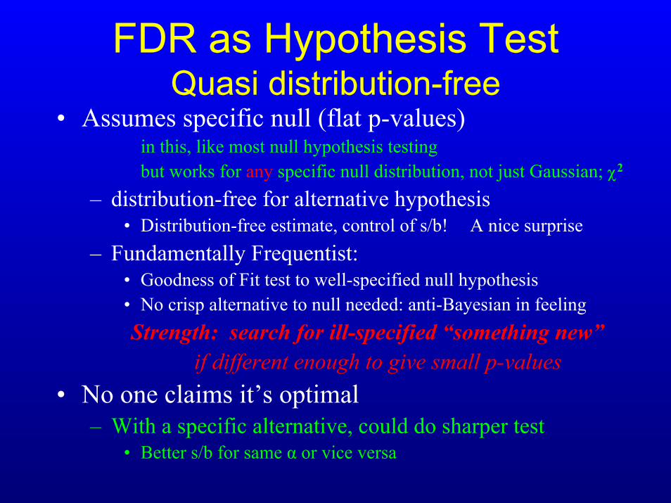
FDR as Hypothesis TestQuasi distribution-free

• Assumes specific null (flat p-values) in this, like most null hypothesis testingbut works for any specific null distribution, not just Gaussian; χ2

– distribution-free for alternative hypothesis• Distribution-free estimate, control of s/b! A nice surprise

– Fundamentally Frequentist: • Goodness of Fit test to well-specified null hypothesis• No crisp alternative to null needed: anti-Bayesian in feelingStrength: search for ill-specified “something new”

if different enough to give small p-values• No one claims it’s optimal

– With a specific alternative, could do sharper test• Better s/b for same α or vice versa

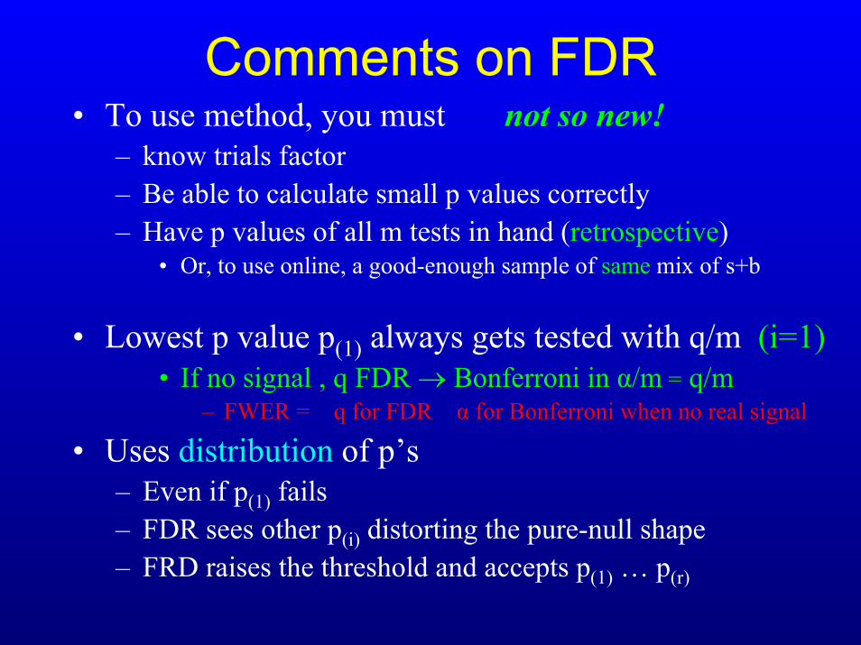
Comments on FDR• To use method, you must not so new!

– know trials factor– Be able to calculate small p values correctly– Have p values of all m tests in hand (retrospective)

• Or, to use online, a good-enough sample of same mix of s+b

• Lowest p value p(1) always gets tested with q/m (i=1)• If no signal , q FDR → Bonferroni in α/m = q/m

– FWER = q for FDR α for Bonferroni when no real signal

• Uses distribution of p’s– Even if p(1) fails– FDR sees other p(i) distorting the pure-null shape – FRD raises the threshold and accepts p(1) … p(r)

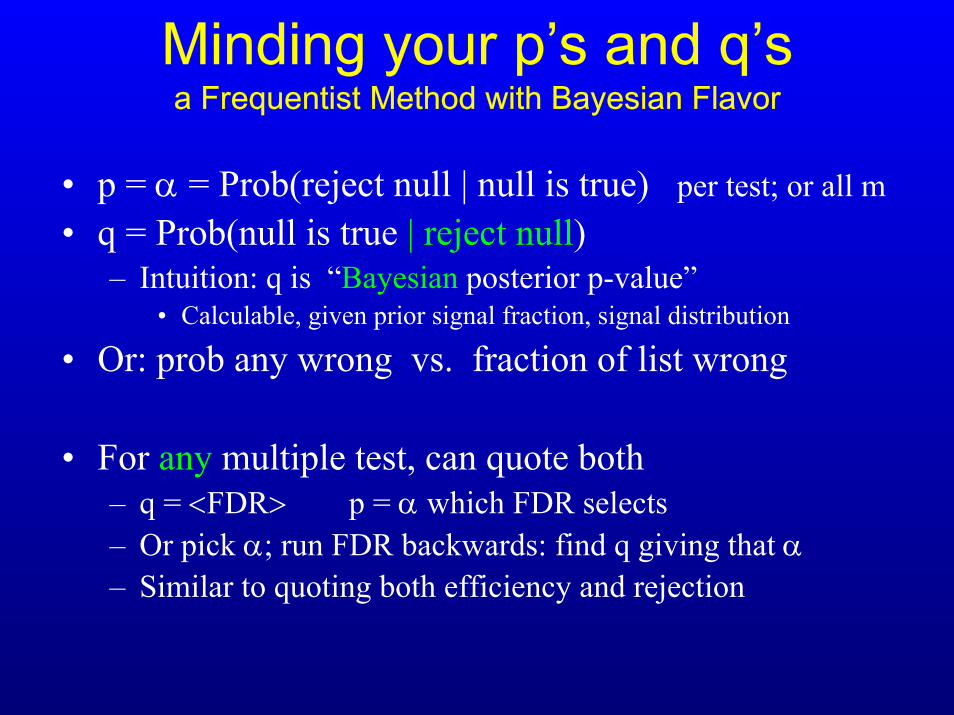
Minding your p’s and q’sa Frequentist Method with Bayesian Flavor

• p = α = Prob(reject null | null is true) per test; or all m• q = Prob(null is true | reject null)

– Intuition: q is “Bayesian posterior p-value”• Calculable, given prior signal fraction, signal distribution

• Or: prob any wrong vs. fraction of list wrong

• For any multiple test, can quote both – q = <FDR> p = α which FDR selects– Or pick α; run FDR backwards: find q giving that α– Similar to quoting both efficiency and rejection

Further Developments

• The statistical literature is under active development:– understand in terms of mixtures (signal + background)

• and Bayesian models of these, or Emperical Bayes

– get better sensitivity by correction for mixture• more important for larger signal strength fractions

– Can estimating FDR in an existing data set, • or FDR with given cuts

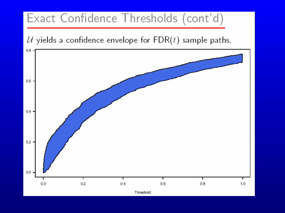
– calculate confidence bands on FDR

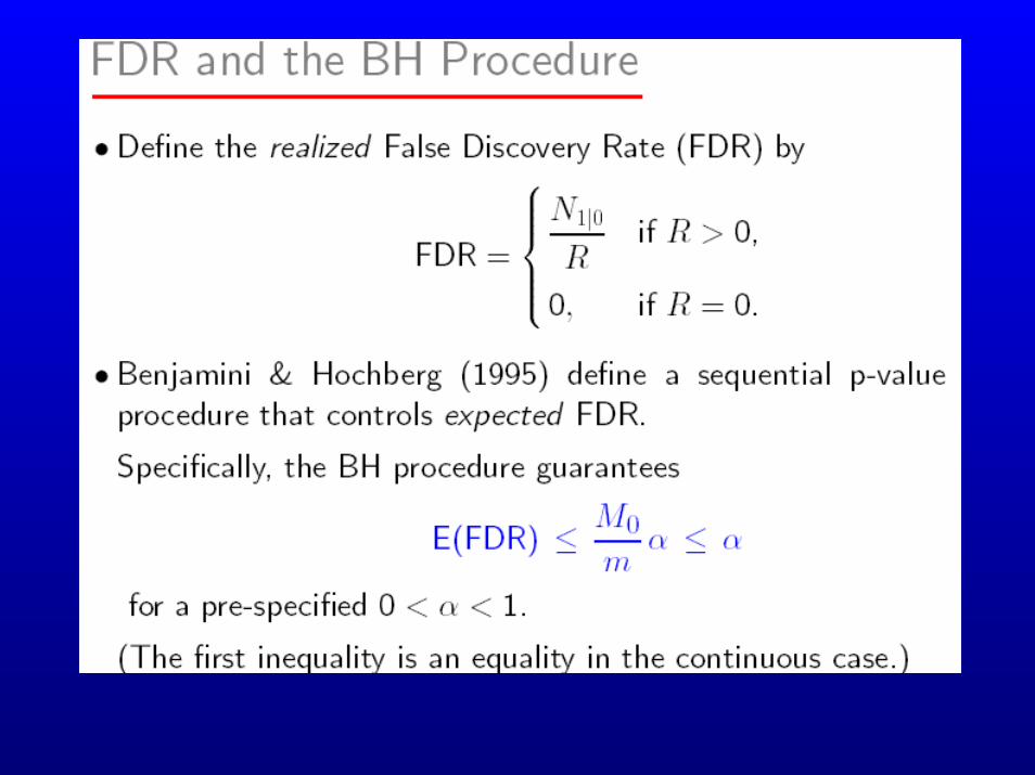
FDR: Conclusions• False Discovery Rate: a new false positive metric

– Control fraction of false positives in multiple measurements– Selects significance cut based on data

• Benjamini & Hochberg FDR Method– Straightforward application to imaging, fMRI, gene searches

– Interesting technique searching for “new” signals• Most natural when expect some signal• But correct control of false positives even if no signal exists• Can report FDR along with significance, no matter how cuts set

– <b> (significance) , and FDR estimate of <s/(s+b)>

– Just one way of controlling FDR• New methods under development e.g. C. Genovese or J. Storey

FDR Talks on WebUsers:– This talk: user.pa.msu.edu/linnemann/public/FDR_Bio.pdf

• 3 more pages of references; and another 30 slides of details

– T. Nichol U Mich www.sph.umich.edu/~nichols/FDR/ENAR2002.pptEmphasis on Benjamini’s viewpoint; Functional MRI

– S. Scheid, MPI cmb.molgen.mpg.de/compdiag/docs/storeypp4.pdfEmphasis on Storey’s Bayesian viewpoint

Statiticians:– C. Genovese CMU www.stat.ufl.edu/symposium/2002/icc/web_records/genovese_ufltalk.pdf

– Y. Benjamini Tel Aviv www.math.tau.ac.il/~ybenja/Temple.ppt

Random Field Theory (another approach to smoothed data)– W. Penny, UCLondon, www.fil.ion.ucl.ac.uk/~wpenny/talks/infer-japan.ppt- Matthew Brett, Cambridge www.mrc-cbu.cam.ac.uk/Imaging/randomfields.html

Some other web pages• http://medir.ohsu.edu/~geneview/education/Multiple test corrections.pdf

Brief summary of the main methods

• www.unt.edu/benchmarks/archives/2002/april02/rss.htmGentle introduction to FDR

www.sph.umich.edu/~nichols/FDR/FDR resources and references—imaging

http://www.math.tau.ac.il/~roee/index.htmFDR resource page by discoverer

Some FDR Papers on WebAstrophysicsarxiv.org/abs/astro-ph/0107034 Miller et. al. ApJ 122: 3492-3505 Dec 2001

FDR explained very clearly; heuristic proof for well-separated signal

arxiv.org/abs/astro-ph/0110570 Hopkins et. Al. ApJ 123: 1086-1094 Dec 20022d pixel images; compare FDR to other methods

taos.asiaa.sinica.edu.tw/document/chyng_taos_paper.pdf FDR comet search (by occultations)will set tiny FDR limit 10-12 ~ 1/year

Statisticshttp://www.math.tau.ac.il/~ybenja/depApr27.pdf Benjamini et al: (invented FDR)

clarifies c(m) for different dependences of dataBenjamani, Hochberg: JRoyalStatSoc-B (1995) 57:289-300 paper not on the web

defined FDR, and Bonferroni-Holm procedurehttp://www-stat.stanford.edu/~donoho/Reports/2000/AUSCFDR.pdf Benjamani et al

study small signal fraction (sparsity), relate to minimax losshttp://www.stat.cmu.edu/www/cmu-stats/tr/tr762/tr762.pdf Genovese, Wasserman

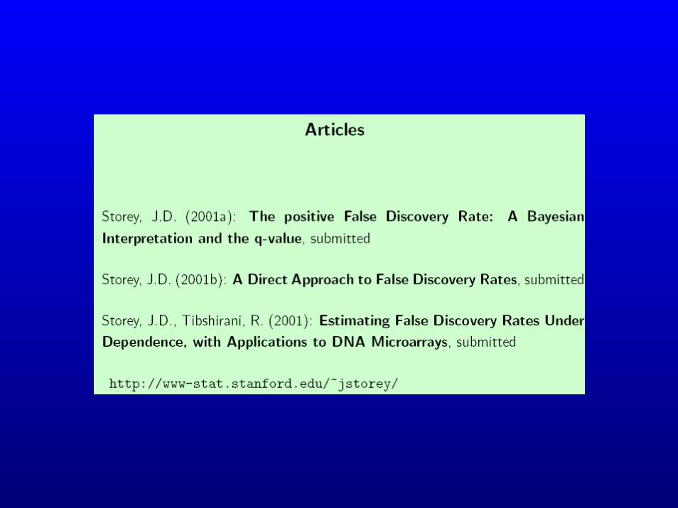
conf limits for FDR; study for large m; another view of FDR as data-estimated method on mixtureshttp://stat-www.berkeley.edu/~storey/ Storey

view in terms of mixtures, Bayes; sharpen with data; some intuition for proofhttp://www-stat.stanford.edu/~tibs/research.html Efron, Storey, Tibshirani

show Empirical Bayes equivalent to BH FDR

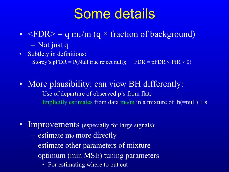
Some details• <FDR> = q mo/m (q × fraction of background)

– Not just q• Subtlety in definitions:

Storey’s pFDR = P(Null true|reject null); FDR = pFDR × P(R > 0)

• More plausibility: can view BH differently: Use of departure of observed p’s from flat:Implicitly estimates from data mo/m in a mixture of b(=null) + s

• Improvements (especially for large signals):– estimate mo more directly– estimate other parameters of mixture– optimum (min MSE) tuning parameters

• For estimating where to put cut

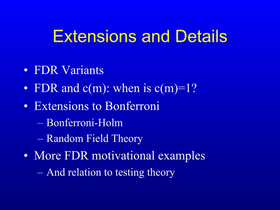
Extensions and Details

• FDR Variants • FDR and c(m): when is c(m)=1?• Extensions to Bonferroni

– Bonferroni-Holm– Random Field Theory

• More FDR motivational examples– And relation to testing theory

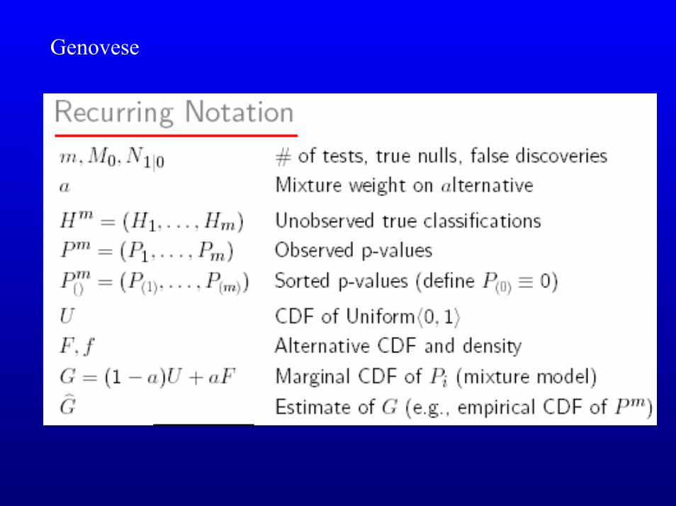
Genovese

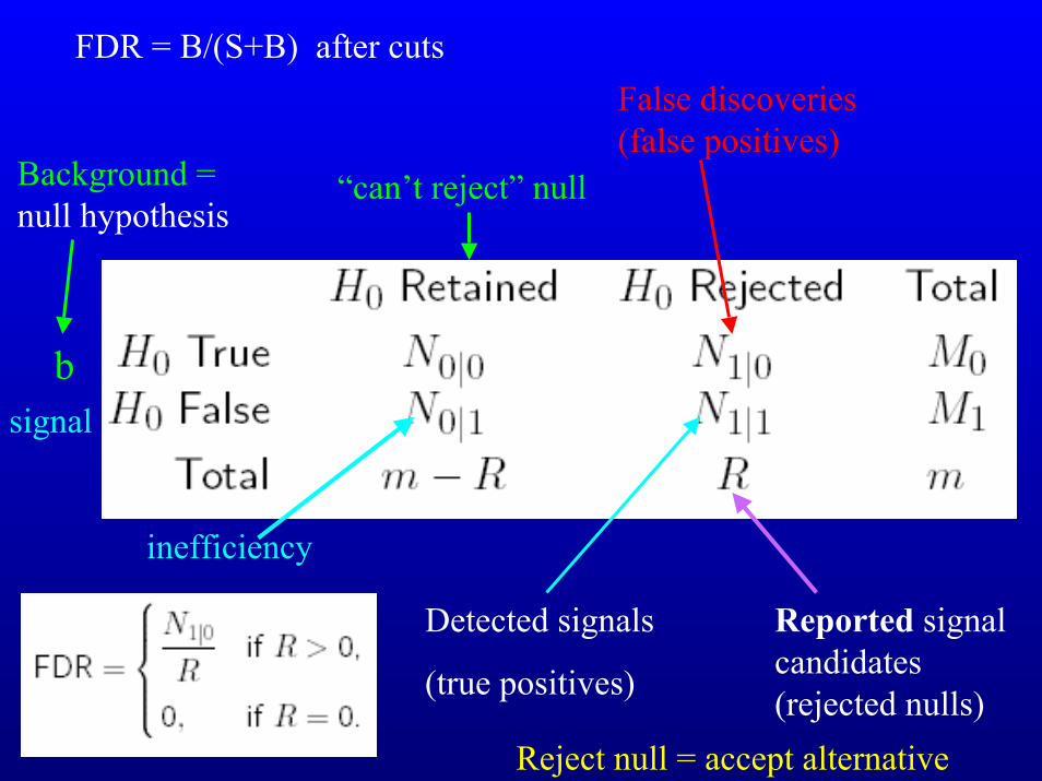
FDR = B/(S+B) after cutsFalse discoveries (false positives)

inefficiency

Background =null hypothesis

“can’t reject” null

bsignal

Reported signal candidates (rejected nulls)

Detected signals

(true positives)

Reject null = accept alternative

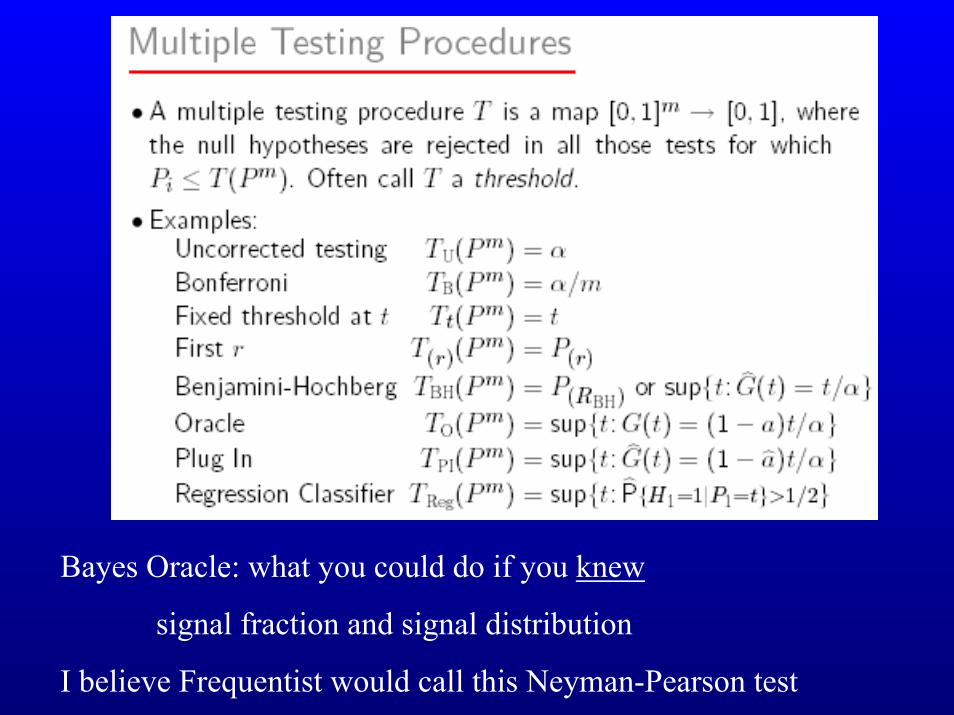
Bayes Oracle: what you could do if you knew

signal fraction and signal distribution

I believe Frequentist would call this Neyman-Pearson test

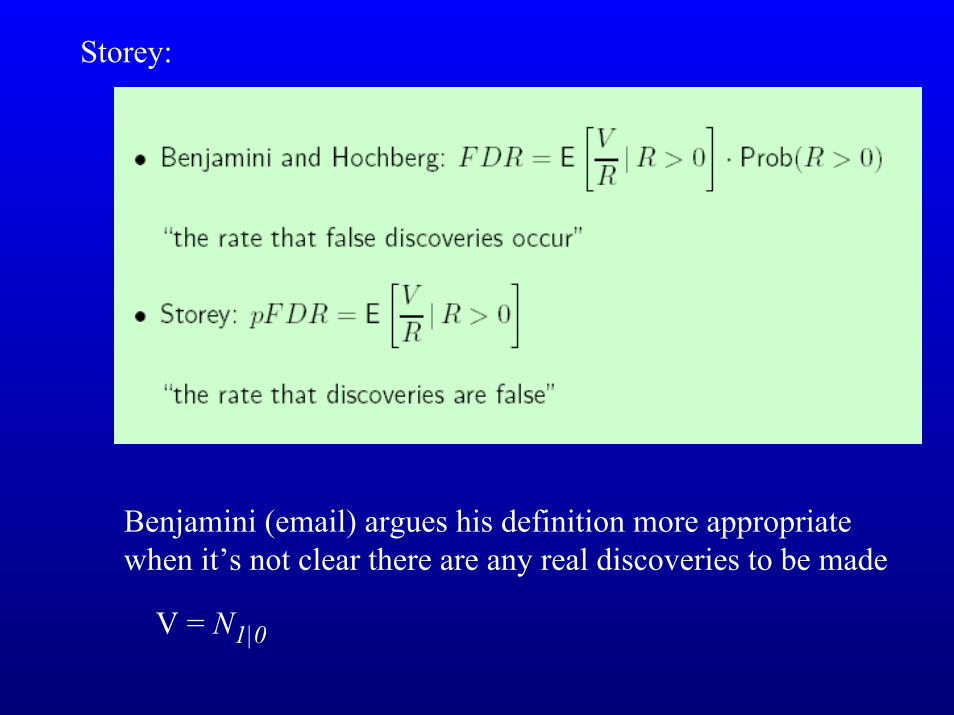
Storey:

Benjamini (email) argues his definition more appropriate when it’s not clear there are any real discoveries to be made

V = N1|0

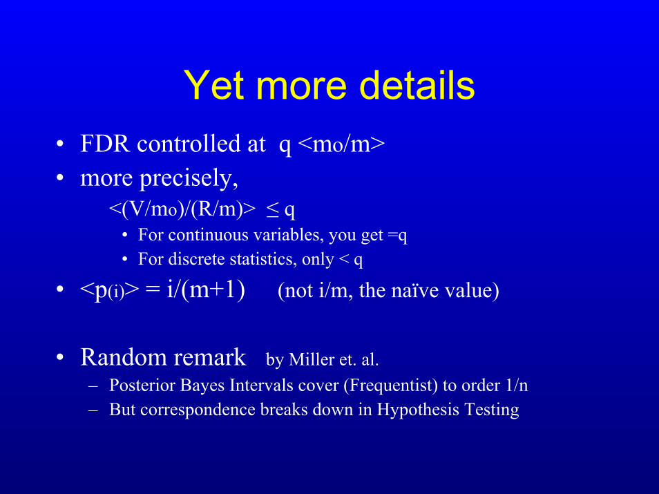
Yet more details• FDR controlled at q <mo/m> • more precisely,

<(V/mo)/(R/m)> ≤ q• For continuous variables, you get =q• For discrete statistics, only < q

• <p(i)> = i/(m+1) (not i/m, the naïve value)

• Random remark by Miller et. al.– Posterior Bayes Intervals cover (Frequentist) to order 1/n– But correspondence breaks down in Hypothesis Testing

Benjamini:

Genovese and Wasserman emphasize the sample quantity V/R

Storey emphasizes E(V/R | R>0)

But both keep the term FDR for their versions

Benjamini & Hochberg c(m) factor

• c(m) = 1– Positive Regression Dependency on Subsets

• Technical condition, special cases include– Independent data– Multivariate Normal with all positive correlations

• Result by Benjamini & Yekutieli, Annals of Statistics, in press.

• c(m) = Σi=1,...m 1/i ≈ log(m)+0.5772– Arbitrary covariance structure

• But this is more conservative—tighter cuts

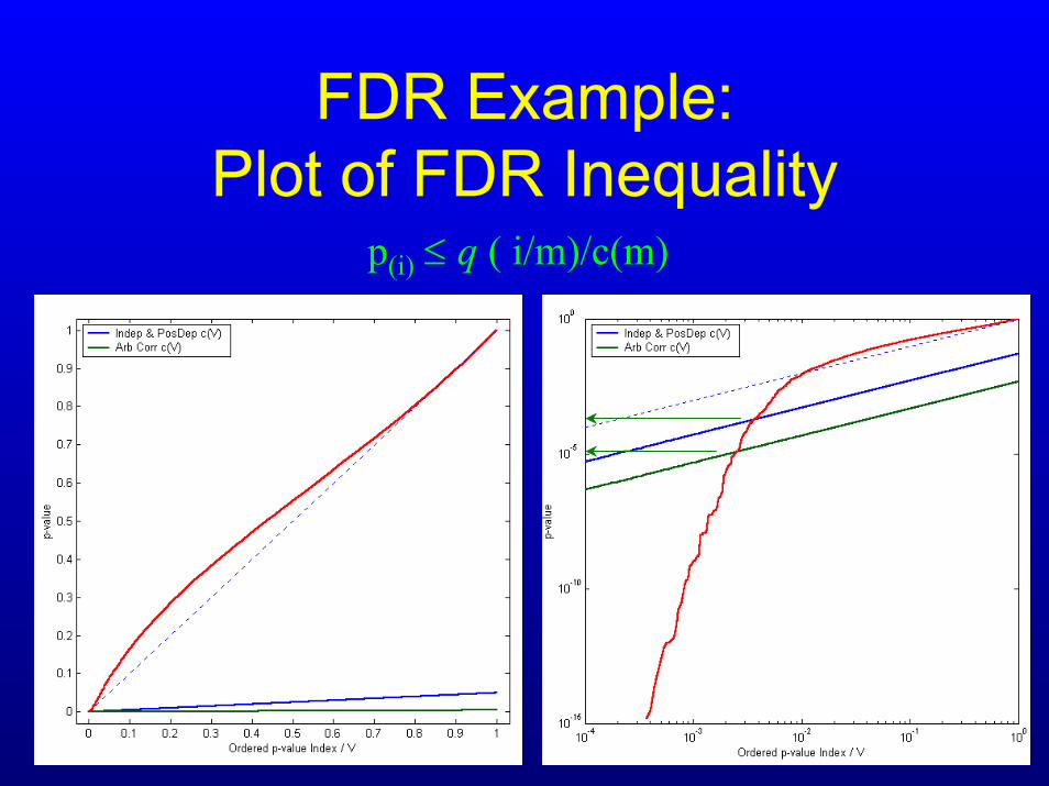
FDR Example:Plot of FDR Inequality

p(i) ≤ q ( i/m)/c(m)

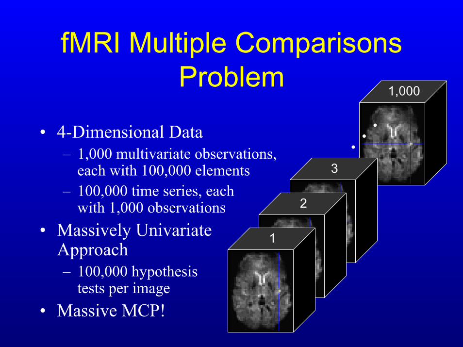
fMRI Multiple Comparisons Problem

• 4-Dimensional Data– 1,000 multivariate observations,

each with 100,000 elements– 100,000 time series, each

with 1,000 observations• Massively Univariate

Approach– 100,000 hypothesis

tests per image• Massive MCP!

1,000

1

2

3

. . .

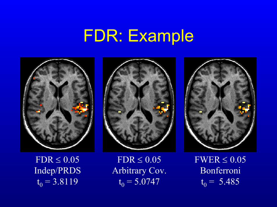
FDR: Example

FDR ≤ 0.05Arbitrary Cov.

t0 = 5.0747

FWER ≤ 0.05Bonferronit0 = 5.485

FDR ≤ 0.05Indep/PRDSt0 = 3.8119

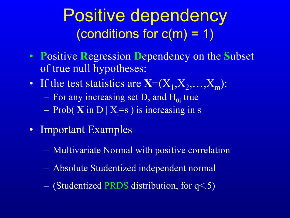
Positive dependency(conditions for c(m) = 1)

• Positive Regression Dependency on the Subset of true null hypotheses:

• If the test statistics are X=(X1,X2,…,Xm):– For any increasing set D, and H0i true– Prob( X in D | Xi=s ) is increasing in s

• Important Examples

– Multivariate Normal with positive correlation

– Absolute Studentized independent normal

– (Studentized PRDS distribution, for q<.5)

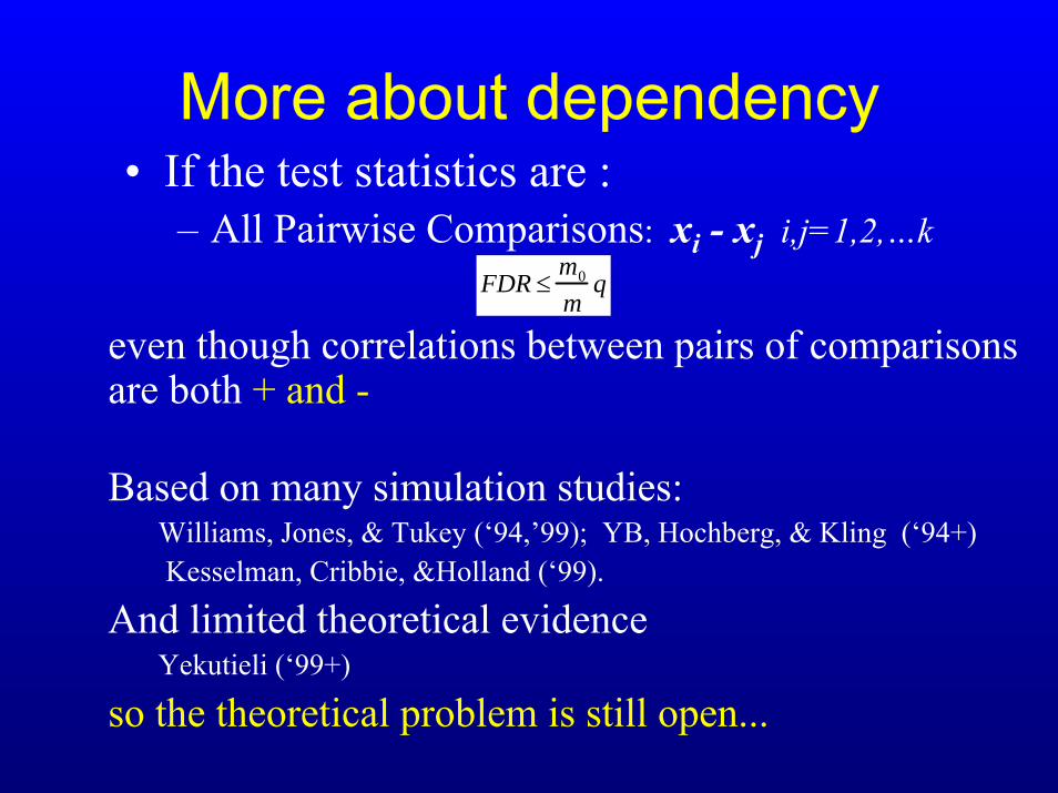
More about dependency• If the test statistics are :

– All Pairwise Comparisons: xi - xj i,j=1,2,…kFDR ≤

m0

mq

even though correlations between pairs of comparisons are both + and -

Based on many simulation studies: Williams, Jones, & Tukey (‘94,’99); YB, Hochberg, & Kling (‘94+) Kesselman, Cribbie, &Holland (‘99).

And limited theoretical evidence Yekutieli (‘99+)

so the theoretical problem is still open...

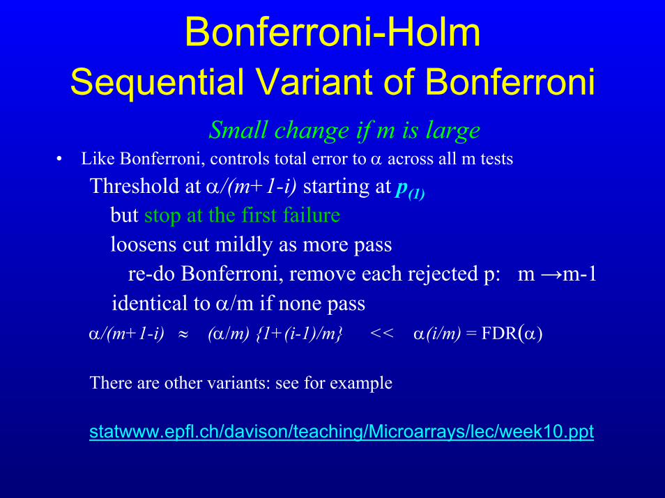
Bonferroni-HolmSequential Variant of Bonferroni

Small change if m is large• Like Bonferroni, controls total error to α across all m tests

Threshold at α/(m+1-i) starting at p(1)but stop at the first failureloosens cut mildly as more pass

re-do Bonferroni, remove each rejected p: m →m-1 identical to α/m if none pass

α/(m+1-i) ≈ (α/m) 1+(i-1)/m << α(i/m) = FDR(α)

There are other variants: see for example

statwww.epfl.ch/davison/teaching/Microarrays/lec/week10.ppt

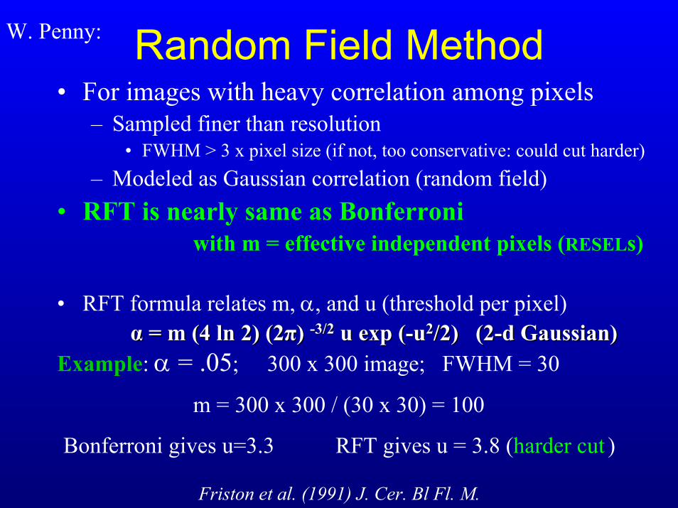
Random Field MethodW. Penny:

• For images with heavy correlation among pixels– Sampled finer than resolution

• FWHM > 3 x pixel size (if not, too conservative: could cut harder)– Modeled as Gaussian correlation (random field)

• RFT is nearly same as Bonferroni with m = effective independent pixels (RESELs)

• RFT formula relates m, α, and u (threshold per pixel)αα = m (4 = m (4 lnln 2) (22) (2ππ) ) --3/23/2 u exp (u exp (--uu22/2) (2/2) (2--d Gaussian)d Gaussian)

Example: α = .05; 300 x 300 image; FWHM = 30

m = 300 x 300 / (30 x 30) = 100

Bonferroni gives u=3.3 RFT gives u = 3.8 (harder cut )

Friston et al. (1991) J. Cer. Bl Fl. M.

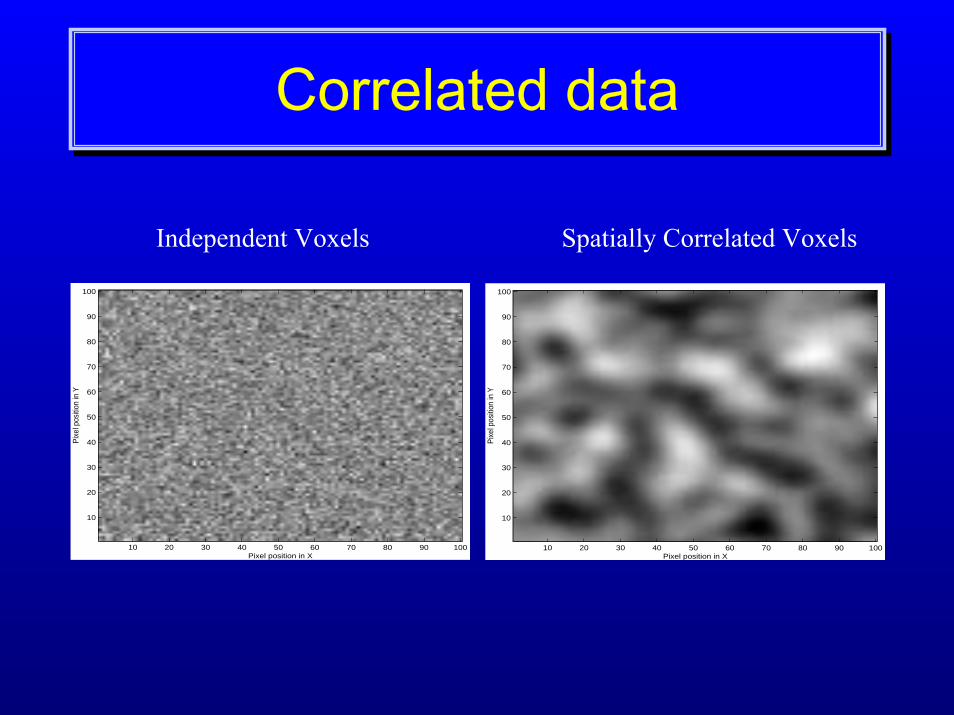
Correlated dataCorrelated data

Pixel position in X

Pix

el p

ositi

on in

Y

10 20 30 40 50 60 70 80 90 100

10

20

30

40

50

60

70

80

90

100

Pixel position in X

Pix

el p

ositi

on in

Y

10 20 30 40 50 60 70 80 90 100

10

20

30

40

50

60

70

80

90

100

Independent Voxels Spatially Correlated Voxels

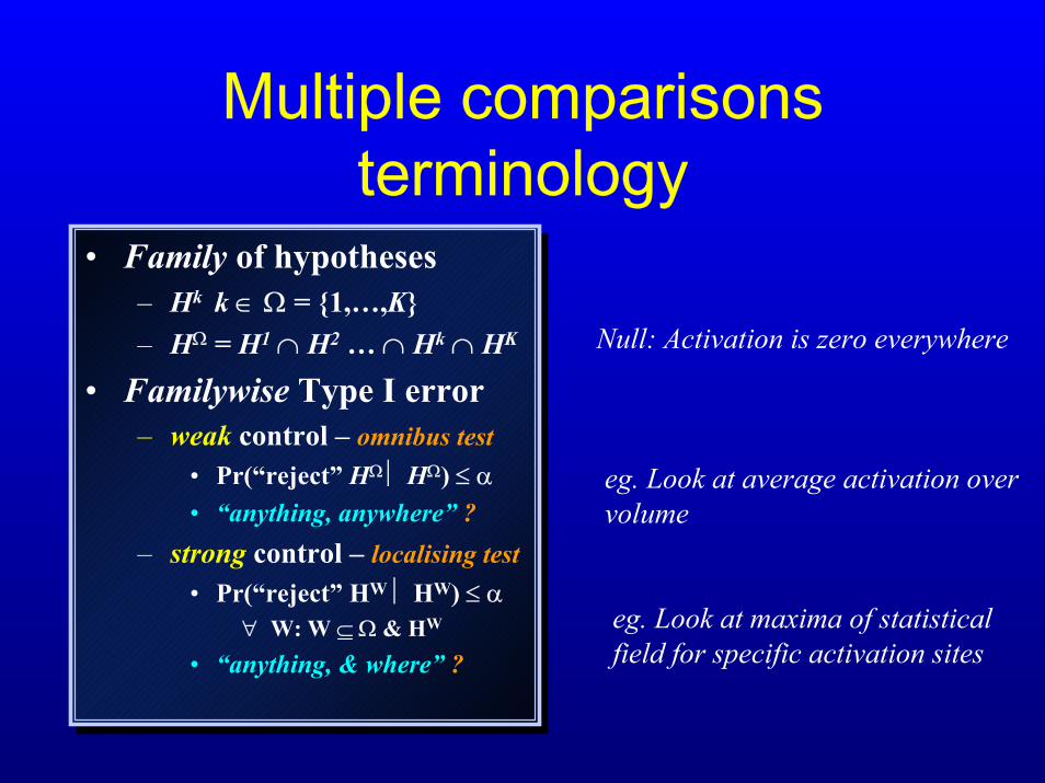
Multiple comparisons terminology

• Family of hypotheses– Hk k ∈ Ω = 1,…,K– HΩ = H1 ∩ H2 … ∩ Hk ∩ HK

• Familywise Type I error– weak control – omnibus test

• Pr(“reject” HΩ HΩ) ≤ α• “anything, anywhere” ?

– strong control – localising test• Pr(“reject” HW HW) ≤ α

∀ W: W ⊆ Ω & HW

• “anything, & where” ?

• Family of hypotheses– Hk k ∈ Ω = 1,…,K– HΩ = H1 ∩ H2 … ∩ Hk ∩ HK

• Familywise Type I error– weak control – omnibus test

• Pr(“reject” HΩ HΩ) ≤ α• “anything, anywhere” ?

– strong control – localising test• Pr(“reject” HW HW) ≤ α

∀ W: W ⊆ Ω & HW

• “anything, & where” ?

Null: Activation is zero everywhere

eg. Look at average activation overvolume

eg. Look at maxima of statisticalfield for specific activation sites

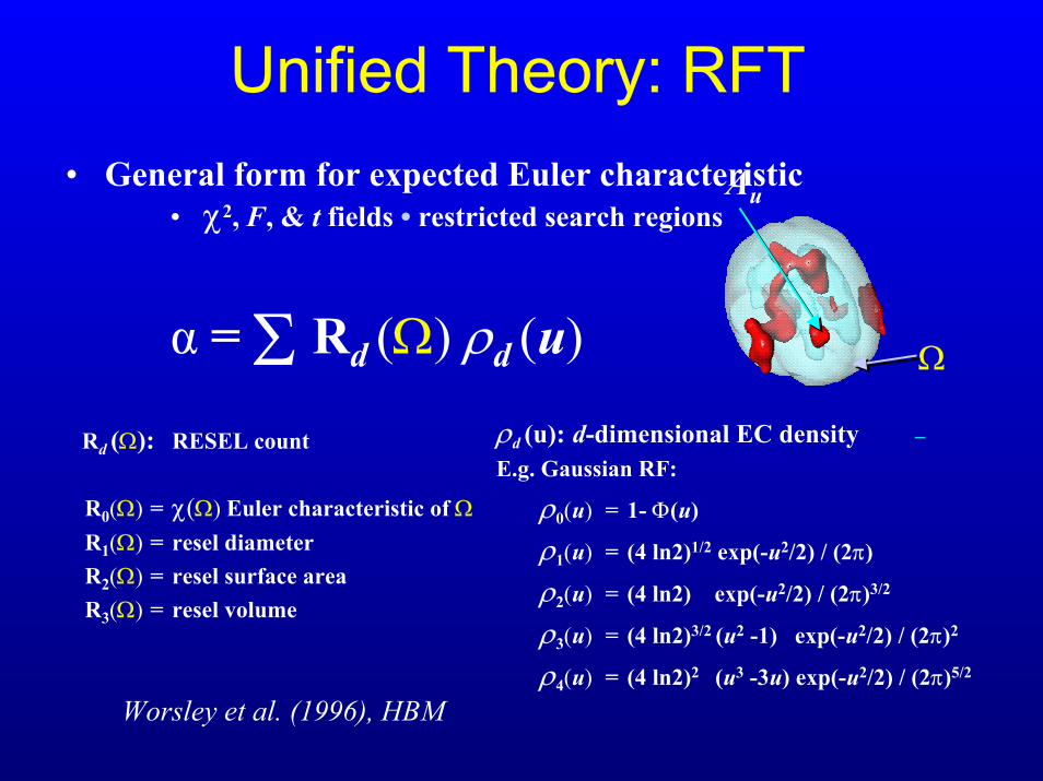
Unified Theory: RFT• General form for expected Euler characteristic

• χ2, F, & t fields • restricted search regions

α = Σ Rd (Ω) ρd (u)

Rd (Ω): RESEL count

R0(Ω) = χ(Ω) Euler characteristic of ΩR1(Ω) = resel diameterR2(Ω) = resel surface areaR3(Ω) = resel volume

ρd (u): d-dimensional EC density –

E.g. Gaussian RF:

ρ0(u) = 1- Φ(u)

ρ1(u) = (4 ln2)1/2 exp(-u2/2) / (2π)

ρ2(u) = (4 ln2) exp(-u2/2) / (2π)3/2

ρ3(u) = (4 ln2)3/2 (u2 -1) exp(-u2/2) / (2π)2

ρ4(u) = (4 ln2)2 (u3 -3u) exp(-u2/2) / (2π)5/2

Au

Ω

Worsley et al. (1996), HBM

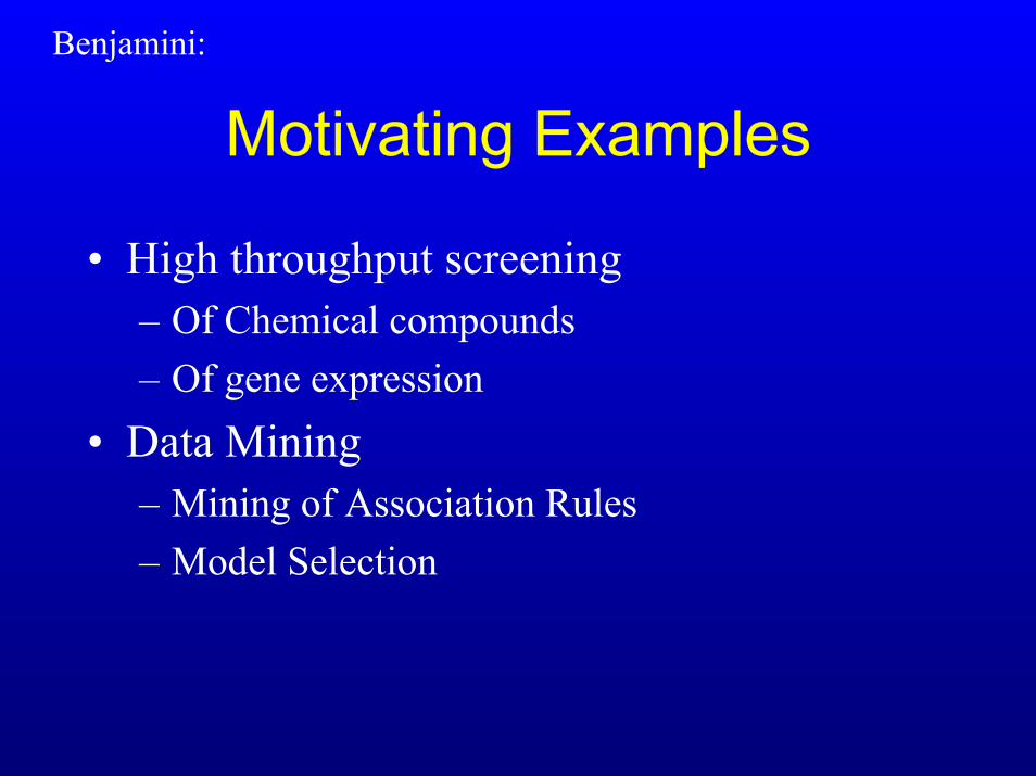
Benjamini:

Motivating Examples

• High throughput screening – Of Chemical compounds– Of gene expression

• Data Mining– Mining of Association Rules– Model Selection

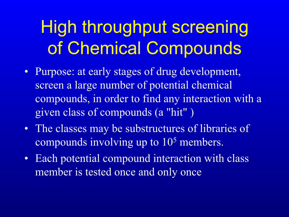
High throughput screening of Chemical Compounds

• Purpose: at early stages of drug development, screen a large number of potential chemical compounds, in order to find any interaction with a given class of compounds (a "hit" )

• The classes may be substructures of libraries of compounds involving up to 105 members.

• Each potential compound interaction with class member is tested once and only once

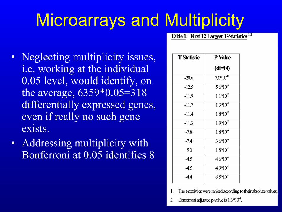
Microarrays and MultiplicityTable 1: First 12 Largest T-Statistics 1,2

T-Statistic P-Value

(df=14) -20.6 7.0*10-12

-12.5 5.6*10-9

-11.9 1.1*10-8

-11.7 1.3*10-8

-11.4 1.8*10-8

-11.3 1.9*10-8

-7.8 1.8*10-6

-7.4 3.6*10-6

5.0 1.8*10-4

-4.5 4.6*10-4

-4.5 4.9*10-4

-4.4 6.5*10-4

1. The t-statistics were ranked according to their absolute values.

2. Bonferroni adjusted p-value is 1.6*10-4.

• Neglecting multiplicity issues, i.e. working at the individual 0.05 level, would identify, on the average, 6359*0.05=318 differentially expressed genes, even if really no such gene exists.

• Addressing multiplicity with Bonferroni at 0.05 identifies 8

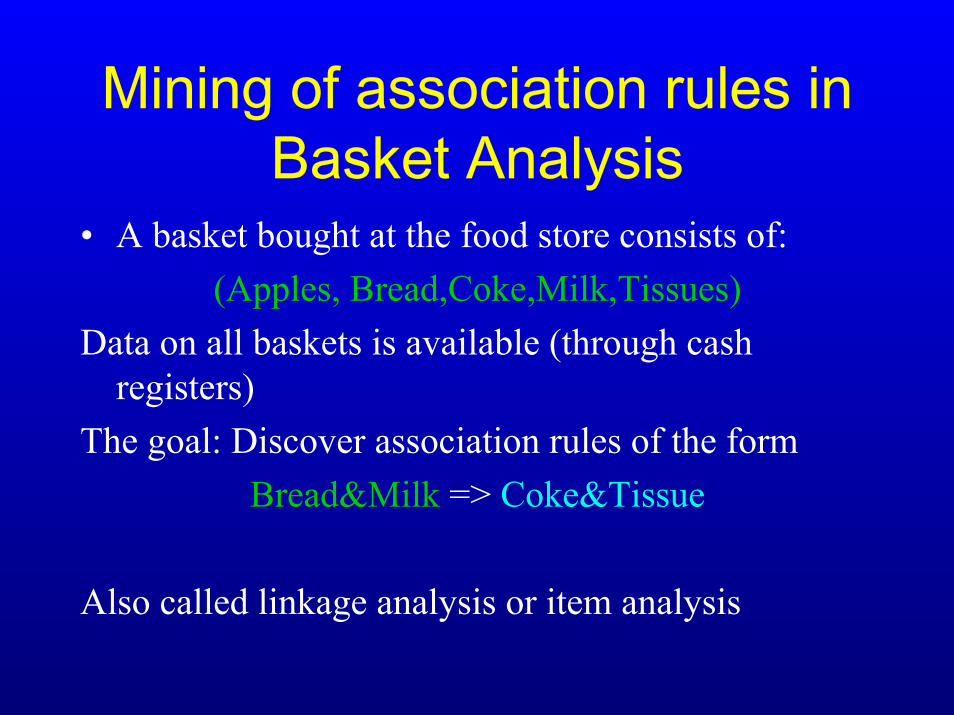
Mining of association rules in Basket Analysis

• A basket bought at the food store consists of:(Apples, Bread,Coke,Milk,Tissues)

Data on all baskets is available (through cash registers)

The goal: Discover association rules of the formBread&Milk => Coke&Tissue

Also called linkage analysis or item analysis

Model Selection

Paralyzed veterans of AmericaMailing list of 3.5 M potential donors200K made their last donation 1-2 years agoIs there something better than mailing all 200K?

– If all mailed, net donation is $10,500– FDR-like modeling raised to $14,700

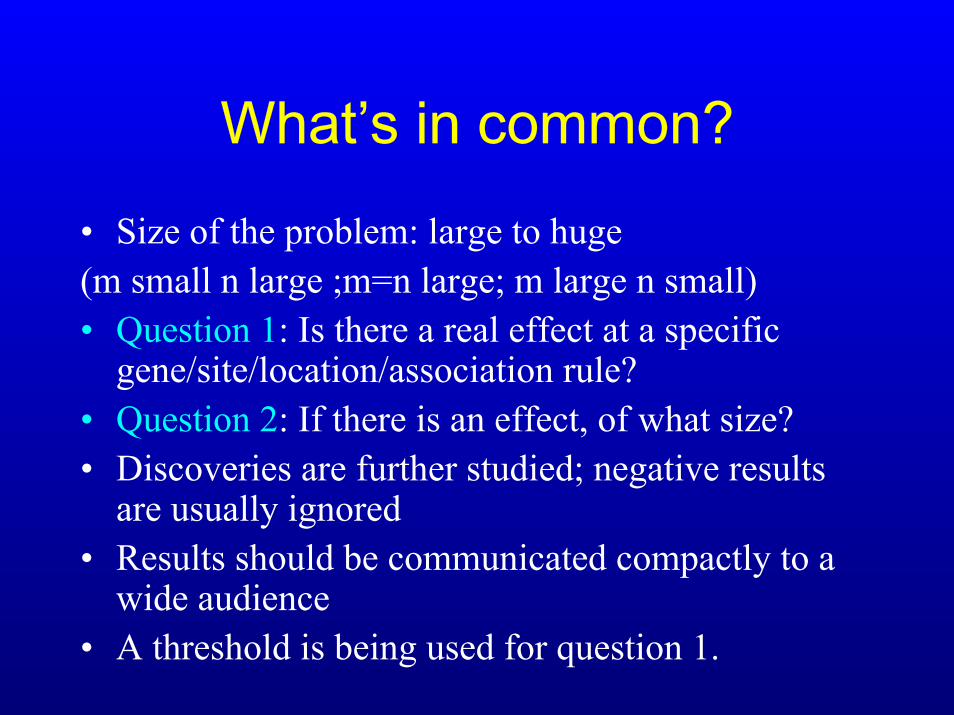
What’s in common?

• Size of the problem: large to huge(m small n large ;m=n large; m large n small)• Question 1: Is there a real effect at a specific

gene/site/location/association rule?• Question 2: If there is an effect, of what size?• Discoveries are further studied; negative results

are usually ignored • Results should be communicated compactly to a

wide audience• A threshold is being used for question 1.

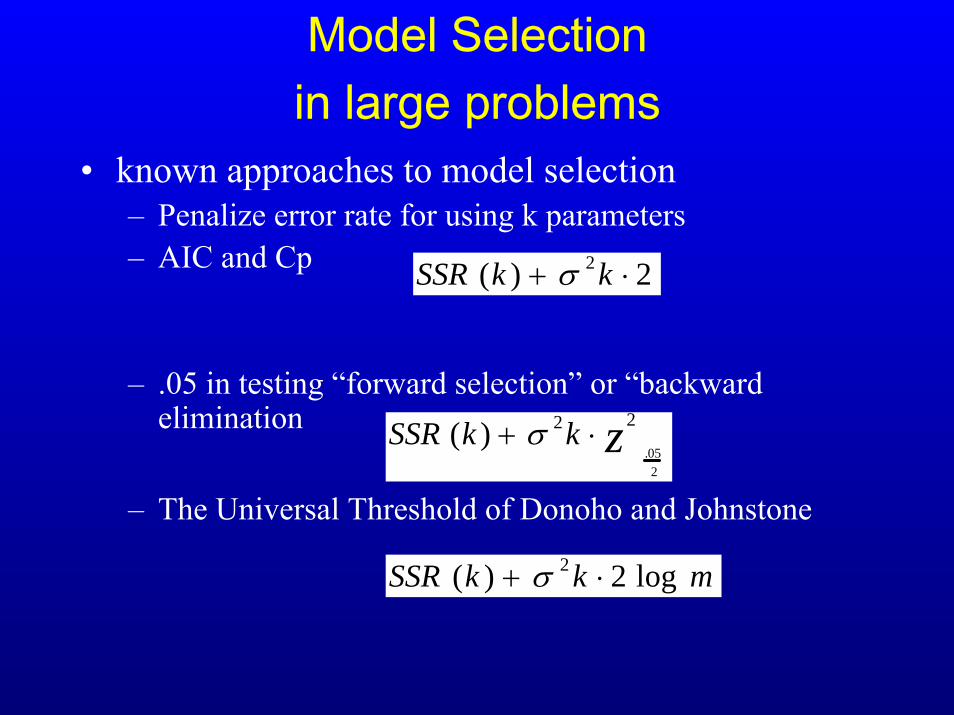
Model Selection in large problems

• known approaches to model selection– Penalize error rate for using k parameters– AIC and Cp

– .05 in testing “forward selection” or “backward elimination

– The Universal Threshold of Donoho and Johnstone

SSR (k ) + σ 2k ⋅2

SSR (k ) + σ 2k ⋅ 2

z .05

2

SSR (k ) + σ 2k ⋅2 log m

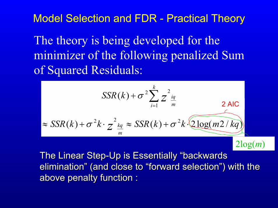
Model Selection and FDR - Practical Theory

The theory is being developed for the minimizer of the following penalized Sum of Squared Residuals:

)/2log(2)()(

)(

222

1

22

kqmkkSSRkkSSR

kSSR

mkq

k

i miq

z

z

⋅+≈⋅+≈

+ ∑=

σσ

σ22 AIC

The Linear StepThe Linear Step--Up is Essentially “backwards Up is Essentially “backwards elimination” (and close to “forward selection”) with the elimination” (and close to “forward selection”) with the above penalty function :

2log(m)

above penalty function :

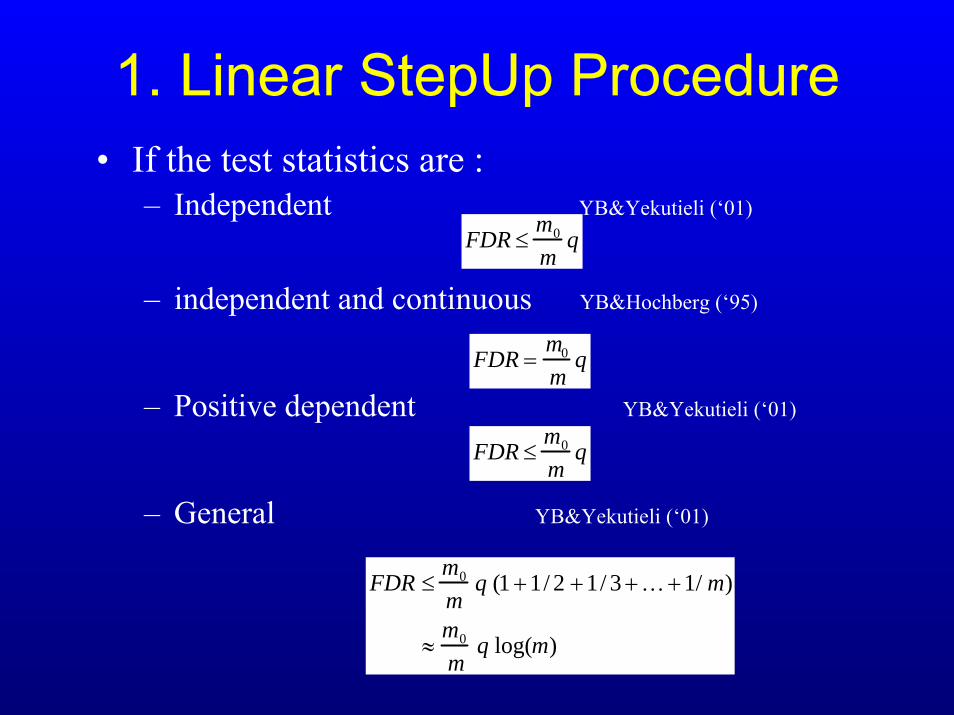
1. Linear StepUp Procedure• If the test statistics are :

– Independent YB&Yekutieli (‘01)

– independent and continuous YB&Hochberg (‘95)

– Positive dependent YB&Yekutieli (‘01)

– General YB&Yekutieli (‘01)

FDR ≤m0

mq

FDR =m0

mq

FDR ≤m0

mq

FDR ≤m0

mq (1 +1/ 2 +1/ 3+K+1/ m)

≈m0

mq log(m)

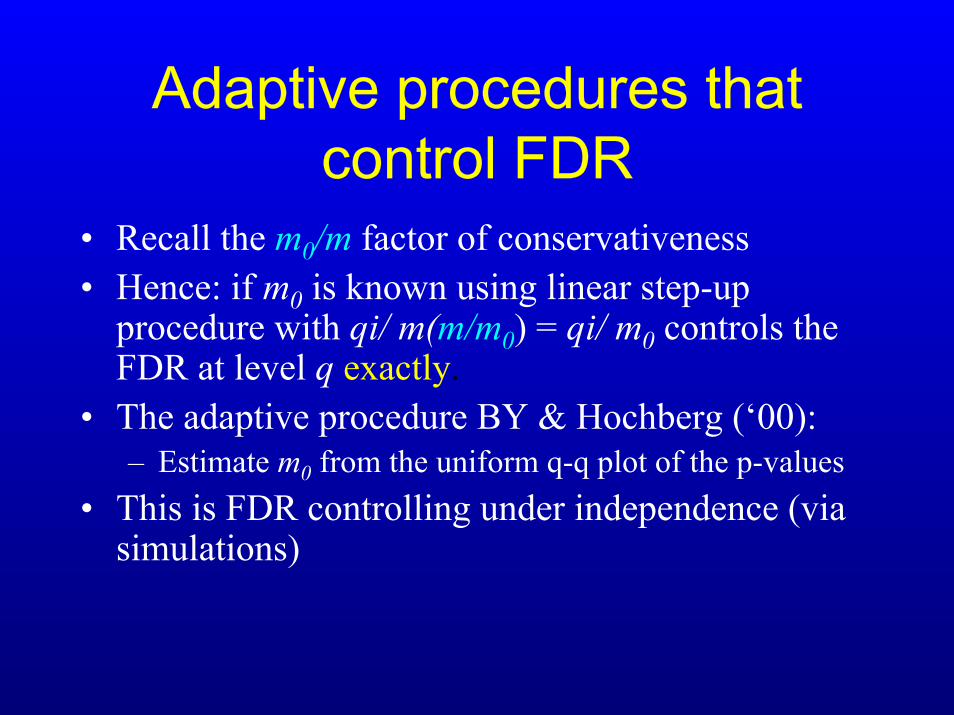
Adaptive procedures that control FDR

• Recall the m0/m factor of conservativeness• Hence: if m0 is known using linear step-up

procedure with qi/ m(m/m0) = qi/ m0 controls the FDR at level q exactly.

• The adaptive procedure BY & Hochberg (‘00): – Estimate m0 from the uniform q-q plot of the p-values

• This is FDR controlling under independence (via simulations)

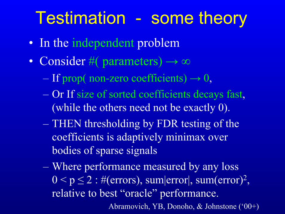
Testimation - some theory• In the independent problem• Consider #( parameters) →∞

– If prop( non-zero coefficients) → 0, – Or If size of sorted coefficients decays fast,

(while the others need not be exactly 0). – THEN thresholding by FDR testing of the

coefficients is adaptively minimax over bodies of sparse signals

– Where performance measured by any loss 0 < p ≤ 2 : #(errors), sum|error|, sum(error)2, relative to best “oracle” performance.

Abramovich, YB, Donoho, & Johnstone (‘00+)