Aalborg Universitet

Controlling a Conventional LS-pump based on Electrically Measured LS-pressure

Pedersen, Henrik Clemmensen; Andersen, Torben Ole; Hansen, Michael Rygaard

Published in:Proceeding of the Fluid Power and Motion Control (FPMC'08)

Publication date:2008

Document VersionPublisher's PDF, also known as Version of record

Link to publication from Aalborg University

Citation for published version (APA):Pedersen, H. C., Andersen, T. O., & Hansen, M. R. (2008). Controlling a Conventional LS-pump based onElectrically Measured LS-pressure. In Proceeding of the Fluid Power and Motion Control (FPMC'08) BathUniversity, The Centre for Power Transmission and Motion Control.

General rightsCopyright and moral rights for the publications made accessible in the public portal are retained by the authors and/or other copyright ownersand it is a condition of accessing publications that users recognise and abide by the legal requirements associated with these rights.

? Users may download and print one copy of any publication from the public portal for the purpose of private study or research. ? You may not further distribute the material or use it for any profit-making activity or commercial gain ? You may freely distribute the URL identifying the publication in the public portal ?

Take down policyIf you believe that this document breaches copyright please contact us at vbn@aub.aau.dk providing details, and we will remove access tothe work immediately and investigate your claim.

Downloaded from vbn.aau.dk on: December 30, 2021

Controlling a Conventional LS-pump based on Electri-cally Measured LS-pressure

Torben O. Andersen Henrik C. Pedersen Michael R. HansenProfessor, Ph.D. Ass. Professor, Ph.D. Asc. Professor, Ph.D.

Energy Technology Energy Technology Mechanical EngineeringAalborg University Aalborg University Aalborg University

DK-9220 Aalborg East DK-9220 Aalborg East DK-9220 Aalborg East+45 9940 9269 +45 9940 9275 +45 9940 9321toa@iet.aau.dk hcp@iet.aau.dk mrh@ime.aau.dk

ABSTRACT

As a result of the increasing use of sensors in mobile hydraulic equipment, the need forhydraulic pilot lines is decreasing, being replaced by electrical wiring and electrically con-trollable components. For controlling some of the existing hydraulic components there are,however, still a need for being able to generate a hydraulic pilot pressure. In this paper con-trolling a hydraulic variable pump is considered. The LS-pressure is measured electricallyand the hydraulic pilot pressure is generated using a small spool valve. From a control pointof view there are two approaches for controlling this system, by either generating a copy ofthe LS-pressure, the LS-pressure being the output, or letting the output be the pump pressure.The focus of the current paper is on the controller design based on the first approach. Specif-ically a controlled leakage flow is used to avoid the need for a switching control structure.

1 INTRODUCTION

The development of hydraulic systems shows a clear tendency towards electrically controlledcomponents, as pointed out by e.g. [1]. This also means that the need for hydraulic pilotlines is decreasing, as load pressures are starting to be measured and distributed electronicallyinstead of hydraulically. However, in the transition phase between traditionally hydraulicallycontrolled components and fully electrically controlled systems, some components may stillneed a hydraulic LS pressure to operate, and there is a need for being able to generate thishydraulic LS pressure based on an electrical reference. One such example is e.g. where a hy-draulic LS-pump is connected to an otherwise electronically controlled system, where thereis no hydraulic LS-pressure available. This problem is the objective of the current paper,where focus is on generating a hydraulic LS-pressure for a conventional variable displace-ment pump.

To the knowledge of the authors, no other such solution has been made; although the prob-lem has some resemblance to controlling the pump pressure in an electronic load sensing

system, which has been the subject of several studies, see e.g. [2, 3, 4, 5, 6, 7]. Commonfor these studies are that they have used a sufficiently fast servo valve/proportional valvedirectly controlling the flow to the displacement piston of the pump. Hence removing theoriginal hydro-mechanical LS-regulator in the pump and in effect replacing the dynamics ofthe hydro-mechanical LS-regulator and pilot line. The idea of using an artificially generatedLS-pressure has also indirectly been presented by [8] as part of a pump regulator, where theLS-pressure was generated based on the pump pressure using a series connection consistingof a fixed orifice and electrically controlled relief valve, hereby obtaining the effect of a pres-sure divider. Apart from the idea of generating the LS-pressure based on the pump pressure,the two solutions do however pose different problems, not only due to different topologiesand control problems, but also as the presented solution is intended to be mounted a distanceaway from the pump and should be applicable in combination with a large variation of pumps.

The paper first presents the considered system and an experimentally verified model. For sta-bility analysis a linearized model is derived and sensitivity of the system to varying operatingconditions discussed. Based on the results of this analysis the controller design is presentedand robustness evaluated. Finally, experimental results are presented, and the performance ofthe electro-hydraulic pressure regulator is compared to that of the hydraulic reference system.

2 SYSTEM MODELLING

The system considered consists of the pump, spool valve, hoses and the load system, as shownin figure 1. From the figure it is seen that the set-up may also be used as a classical LS-system(parallel circuit), making it possible to test the two systems individually.

PB

PA

PtPp

LoadLS Pump PR Valve PVG32

PLS

Figure 1: Diagram of the experimental set-up with indication of the various compo-nents.

The system consists of a 57[cm3] Sauer-Danfoss series 45 H-frame pump, a load system con-sisting of a PVG 32 pressure compensated proportional valve, two variable orifices connected

in parallel and an on-off valve. The spool valve (Pressure Regulating-valve) used is a 3/3-NCunder lap valve. The PR-valve is actuated with a voice coil connected to a DC/DC inverter,by which the voice coil may be current controlled.

2.1 Pressure regulating valve

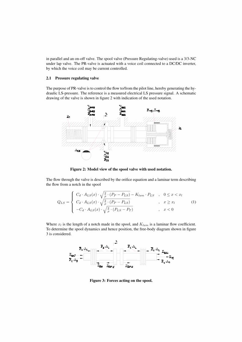
The purpose of PR-valve is to control the flow to/from the pilot line, hereby generating the hy-draulic LS-pressure. The reference is a measured electrical LS pressure signal. A schematicdrawing of the valve is shown in figure 2 with indication of the used notation.

Figure 2: Model view of the spool valve with used notation.

The flow through the valve is described by the orifice equation and a laminar term describingthe flow from a notch in the spool

QLS =

Cd ·ALS(x) ·

√2ρ · (PP − PLS)−Klam · PLS , 0 ≤ x < xl

Cd ·ALS(x) ·√

2ρ · (PP − PLS) , x ≥ xl

−Cd ·ALS(x) ·√

2ρ · (PLS − PT ) , x < 0

(1)

Where xl is the length of a notch made in the spool, and Klam is a laminar flow coefficient.To determine the spool dynamics and hence position, the free-body diagram shown in figure3 is considered.

Figure 3: Forces acting on the spool.

From the figure it may be seen that the spool is pressure balanced. The force equilibrium forthe spool may therefore be written as:

mspool · x = FV C + Fspr − Fflow,p + Fflow,t − Ffric (2)

where mspool is the movable mass (including voice coil etc.). Fspr = xspool · (k1 − k2) +Fspr,0 is the spring force, Fflow,p and Fflow,t are the flow forces for the pump side and tankside valve openings respectively and Ffric is the friction force. FV C is the voice coil force,which is proportional to the current in the voice coil, which again may be found from thevoltage equation, i.e.

uV C = RV CiV C + LV Cdi

dt+ Kmx (3)

FV C = Km · iV C (4)

where Kmx is the back emf and Km is the voice coil force constant.

The friction force is modelled as a combination of stiction, Coulomb and viscous friction as

Ffric =

{FV C + Fspr − Fflow,p + Fflow,t , x = 0 ∧ FV C + Fspr − Fflow,p + Fflow,t < Fs

Fc · sign(x) + B · x , |x| > 0(5)

Where Fc is the Coulomb friction, Fs the stiction force and B the viscous friction coefficient.Finally, the flow forces are modelled as purely stationary flow forces, i.e. for the pump side

Fflow,p = 2 · Cd ·ALS(s) · (PP − PLS) · cos(θ) (6)

and similarly for the tank side opening.

2.2 Pump, Volumes and Load Models

The other components in the system considered include the pump, volumes (hoses) and theload model. Considering first the different volumes in the system, these are generally de-scribed using the continuity equation, which for the LS-hose volume yields:

VLS

β

dp

dt+

dVLS

dt= Qin −Qout (7)

With Qin and Qout being the flows in and out of the volume and β the effective oil bulkmodulus. The latter is modelled as being pressure dependent as described in e.g. [9]. Theload consists of the two variable orifices, which are simply described by the orifice equation,whereas the on-off valve is simply modelled as a switch. The load is here only used togenerate a load pressure for a given pump flow. As described earlier the pump is a Sauer-Danfoss series 45 H-frame pump. The model is quite comprehensive and is presented in[10].

0 1 2 3 4 50

10

20

30

40

50

60

70

80

Time [s]

Pre

ssur

e [b

ar]

PP test

PLS

test

PP sim

PLS

sim

0 1 2 3 4 50

10

20

30

40

50

60

Time [s]

Pre

ssur

e [b

ar]

PA test

PB test

PA sim

PB sim

0 1 2 3 4 570

75

80

85

90

Time [s]

Flo

w [L

/min

]

QA−B

test

QA−B

sim

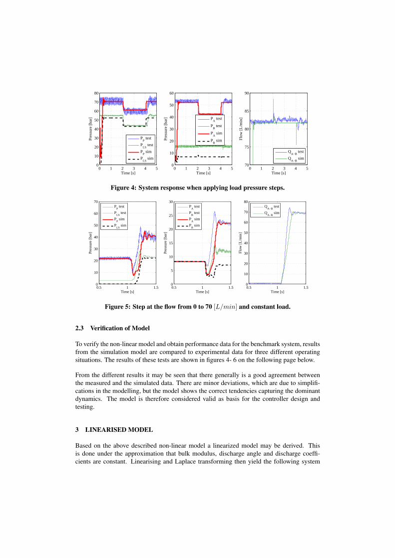
Figure 4: System response when applying load pressure steps.

0.5 1 1.50

10

20

30

40

50

60

70

Time [s]

Pre

ssur

e [b

ar]

P

P test

PLS

test

PP sim

PLS

sim

0.5 1 1.50

5

10

15

20

25

30

Time [s]

Pre

ssur

e [b

ar]

P

A test

PB test

PA sim

PB sim

0.5 1 1.50

10

20

30

40

50

60

70

80

Time [s]

Flo

w [L

/min

]

Q

A−B test

QA−B

sim

Figure 5: Step at the flow from 0 to 70 [L/min] and constant load.

2.3 Verification of Model

To verify the non-linear model and obtain performance data for the benchmark system, resultsfrom the simulation model are compared to experimental data for three different operatingsituations. The results of these tests are shown in figures 4- 6 on the following page below.

From the different results it may be seen that there generally is a good agreement betweenthe measured and the simulated data. There are minor deviations, which are due to simplifi-cations in the modelling, but the model shows the correct tendencies capturing the dominantdynamics. The model is therefore considered valid as basis for the controller design andtesting.

3 LINEARISED MODEL

Based on the above described non-linear model a linearized model may be derived. Thisis done under the approximation that bulk modulus, discharge angle and discharge coeffi-cients are constant. Linearising and Laplace transforming then yield the following system

0 1 2 3 40

10

20

30

40

50

60

70

Time [s]

Pre

ssur

e [b

ar]

P

P test

PLS

test

PP sim

PLS

sim

0 1 2 3 40

5

10

15

20

25

30

35

40

Time [s]

Pre

ssur

e [b

ar]

P

A test

PB test

PA sim

PB sim

0 1 2 3 40

10

20

30

40

50

60

Time [s]

Flo

w [L

/min

]

Q

A−B test

QA−B

sim

Figure 6: Sinusoidal input with frequency of 1 [Hz].

equations:

mspool · s2 · x = Kf · iV C −Kspr,fq · x + Kfqppt · PLS + Kfqpp · Pp −B · s · x (8)qLS = Kqpt · x− (Kqppt + Klam) · pLS + Kqpp · pp (9)

pLS =β

s · VLS· qLS (10)

uV C = RV C · iV C + LV C · s · iV C + Kg,V C · s · x (11)

The first expression here describe the linearised spool force equilibrium, the second the flowto the LS-hose, the third the pressure build up in the LS-hose and the fourth the voice coildynamics. Combining these equations in block diagram form, the block diagram shown infigure 7 may be obtained.

Figure 7: Block diagram relating valve voltage input (up,LS) to pressure in the LS-line(pLS).

In the block diagram the term, Gp(s), represents the pump and pump volume dynamics. Asa rough approximation this is modelled by a first order filter:

Gp(s) =pp

pLS=

1τp · s + 1

(12)

To simplify the following analysis, the system may be considered in two different situations,where in the first the valve opens for connection between pump volume and the LS-hose(pump side connection), whereas in the second situation the valve opens to tank. As thesystem is current controlled the analysis is further simplified. For the case where the valveopens to the pump side the transfer function for the system may then be found to be

GLS,p(s) =pLS

iV C=

βKq,ptKf (τps + 1)

Gd(s) (mspools2 + Bs + Kspr,fq) − (τps + 1) βKqp,tKfqp,pt − βKq,ptkfqp,p

(13)where Gd(s) = ((VLSs + βKqp,t + βKleak) (τps + 1)− βKqp,p). For the tank side con-nection case the system transfer function reduces to:

GLS,t(s) =βKq,ptKf

(VLSs + βKqp,t + βKleak) (mspools2 + Bs + Kspr,fq)− βKq,ptKfqp,pt

(14)

4 STABILITY AND SENSITIVITY ANALYSIS

In order to determine a control strategy for the system, it must be determined under whichoperating conditions the system is likely to become unstable. The main influence is due to thepressure drop over the spool valve, ∆p, the spool position, x, and the pump time constant, τp

(dependent on pump volume and pump type). In order to investigate this influence the polesvariations for varying operating conditions are investigated by looking at pole variations.

4.1 Pump side

The open loop pump side transfer function given in eq. (13) has four poles and one zero. Thezero originates from the pump dynamics, always being in the left half plane and hence beingof no interest at this point. Therefore, only the movement of the four poles is considered.The results of varying the pressure drop over the spool and the spool travel are shown in thefigures (8) and (9).

From these results it may be seen that increasing the pressure drop1 over the spool does nothave a major influence on the dominating poles, but does mean that the damping is decreased.Increasing the spool position does however have major influence on the dominant dynamics,where large spool movements may actually lead to an unstable system in combination withthe highest pressure drops. In reality it is, however, very unlikely that these worst case operat-ing points may ever be reached, as a full spool travel in combination with the highest possiblepressure drop of 18 [bar] will yield unrealistic operation conditions. From simulations withthe non-linear model described in section 2, it has been found that realistic flow requirementsare around 1.35[l/min]. Plotting the pole locations for varying pressure drop and spool dis-placement yields the plot shown in figure 10 when ensuring a flow of 1.35[l/min] . Basedon this plot, the worst case working point for the pump side is therefore found to be for apressure drop of ∆p = 18[Bar] and a spool displacement x = 0.277[mm].

1The pressure drop cannot exceed the pressure margin of the pump, which is 18[bar].

−200 −180 −160 −140 −120 −100 −80 −60 −40 −20 0−600

−400

−200

0

200

400

600

Real Axis

Imag

inar

y ax

is

Figure 8: Pole movement for pressure drop ∆p = pp − pLS ∈ [1− 18] [bar].

−1000 −800 −600 −400 −200 0 200−800

−600

−400

−200

0

200

400

600

800

Real Axis

Imag

inar

y ax

is

Figure 9: Pole movement at ∆p = pp − pLS = 18[bar] and spool position from x ∈[0.01− 2.5] [mm].

4.2 Tank side

For the tank side the transfer function defined in eq. (14) has three poles and no zeros. Asoppose to the pump side, the pump and pump volume dynamics is not influencing the tankside dynamics and hence the linearisation point will only be dependent on the pressure dropover spool (∆p = pLS − pT ) and the spool position. The pressure drop over the spool is, onthe other hand, only bounded by the maximum pressure in the system, why the pressure dropin opening situation may be very large. The stability and damping of the system for varying

−300 −250 −200 −150 −100 −50 0−800

−600

−400

−200

0

200

400

600

800

Real Axis

Imag

inar

y ax

is

Figure 10: Pole movement at 1.35 [l/min] for rising pressure and hence decreasing spooldisplacement.

pressure drop and spool opening may be seen in figures 11 and 12.

Figure 11: Pole movement for pressure drop 1-250 [bar].

For the higher pressure drops (> 30[bar]) the system has one of the poles in the right halfplane and is therefore unstable. As for the pump side the worst case operating point is for the

1

2

Figure 12: Pole movement at 250 [bar] and spool position from 0.01-2.5 [mm].

highest possible pressure drop and the flow requirement of 1.35[l/min]. This correspond to∆p = 250[bar] and x = 0.114[mm].

4.3 Sensitivity to varying LS-Hose Volume

The LS-hose volume directly influences the (open loop) system gain, i.e. the larger the vol-ume, the lower the system gain. To illustrate this influence on the stability, the pole locationas a function of the LS-hose volume is shown in figure 13 for the pump side case and figure14 for the tank side case. The variations are made for VLS ∈ [20[ml], 320[ml]].

−250 −200 −150 −100 −50 0−600

−400

−200

0

200

400

600

Imag

inar

y ax

is

Real axis

Figure 13: Open-loop poles location on pump side when considering LS-hose volumevariations.

−1500 −1000 −500 0 500 1000 1500−1

−0.5

0

0.5

1

Imag

inar

y ax

is

Real axis

Figure 14: Open-loop poles location on tank side when considering LS-hose volumevariations.

As expected the dominant system eigen frequency is lowered and the damping increased forthe pump side when the volume is increased, and hence the system becomes slower. For thetank side the variation of the LS-volume is of minor influence.

5 CONTROLLER DESIGN

The basic demands of the system are that the performance must be comparable to that ofthe benchmark system, and that the control system is robust to changes in the system layout,i.e. hose volumes and pump type. Basically, as the system structure changes dependent onthe spool position (i.e. open between pump side and LS-hose or between LS-hose and tankside), two controllers should be considered - one for each opening situation. Utilising thistype of control structure, however, requires correct handling of the transition situation, wherethe spool crosses the zero position and the system structure changes. The situation is furthercomplicated by the fact that the tank side dynamics is very sensitive to the pressure in the LShose, and even becomes unstable for a pressure drop above approximately 30 bars, as shownin the previous sections. One way to overcome the switching problems is to use a kind ofpressure dividing, by making a notch in the spool, allowing flow to pass from the LS hoseto tank. By proper design of the area characteristic of the notch, crossing the zero positionwill only take place when the LS pressure is small (less than approximately 30 bars), i.e. weneed to dump a relatively large amount of flow. In this situation the tank side dynamics willbe stable and we can handle both situations with the same controller. Also, by allowing thespool to cross the zero position will decrease the loss inevitable arising from the ”leakage”flow.

The system dynamics can now in both cases approximately be described by a relatively welldamped third order system. However, the flow from the notch will change the system typefrom being a type 1 to being a type 0 system. Based on these considerations a standardPI-controller is utilised.

Gcp(s) = 0.69 ·(

1 +1

1.5 · s

)(15)

The open-loop bode plot of the system with applied PI-controller is shown in figure 15.

100

101

102

103

104

−270

−225

−180

−135

−90

P.M.: 68.1 degFreq: 62 rad/sec

Frequency (rad/sec)

Pha

se (

deg)

−100

−50

0

50

G.M.: 12 dBFreq: 598 rad/secStable loop

Mag

nitu

de (

dB)

Figure 15: Open-loop bode plot of the pump side with the PI-controller. The circles andcrosses representing respectively the zeros and the poles of the system, with the the firstcircle (red) resulting from the zero added by the PI-controller.

Based on the above analysis the designed controller has been implemented and tested exper-imentally. The results are shown in figures 16-18.

1 1.5 2 2.5 3 3.5 4 4.5 5 5.5 60

5

10

15

20

25

30

35

40

Time [s]

Pres

sure

[ba

r]

P

Pump

PLS

PRef

1 1.5 2 2.5 3 3.5 4 4.5 5 5.5 6−0.05

−0.04

−0.03

−0.02

−0.01

0

0.01

0.02

0.03

0.04

0.05

Time [s]

Pos

ition

[mm

]

Position

Figure 16: Measured pressure and spool position when operating at low pressures andapplying pressure steps.

From the results it may be seen that the system is operating as expected. For small pressuresteps the system is continuously operating with a positive spool position, as seen in Fig. 17,meaning that the system is continuously controlling the leakage flow to tank. For the larger

1 1.5 2 2.5 3 3.5 4 4.5 5 5.5 670

75

80

85

90

95

100

105

110

115

120

Time [s]

Pres

sure

[ba

r]

P

Pump

PLS

PRef

1 1.5 2 2.5 3 3.5 4 4.5 5 5.5 6−0.01

0

0.01

0.02

0.03

0.04

0.05

0.06

0.07

0.08

Time [s]

Pos

ition

[mm

]

Position

Figure 17: Measured pressure and spool position when operating at high load pressureand applying minor pressure steps.

1 1.5 2 2.5 3 3.5 4 4.5 5 5.5 620

30

40

50

60

70

80

90

100

110

Time [s]

Pres

sure

[ba

r]

P

Pump

PLS

PRef

1 1.5 2 2.5 3 3.5 4 4.5 5 5.5 6

−0.1

−0.05

0

0.05

0.1

Time [s]

Pos

ition

[mm

]

Position

Figure 18: Measured data for high load pressure and large pressure steps.

downwards pressure steps and when operating at low system pressure (Fig. 18 and 16 re-spectively), the leakage flow is however not large enough, to swash out the pump sufficientlyfast, why the valve switches over and operates with a negative spool position. In this case thepressure drop over the spool have, however been lowered (due to the initial leakage flow), toa level where the system is not unstable, cf. the above analysis.

6 CONCLUSION

The focus of this paper has been on generating a hydraulic (LS) pilot pressure based onan electric reference for use in systems without hydraulic feedback of the load pressure.This was done using a small spool valve, where a model of the valve and the consideredsystem was first presented. A linear analysis of the system yielded the worst case operatingconditions of the system, and based on this analysis an approach using a controlled leakageflow was utilised, hereby enabling the system to be operated with a simple PI-controller andstill be stable and robust towards transitions between pump and tank side operation. Finallyexperimental results were presented showing the validity of the approach.

References

[1] H.H. Harms. Hydraulic fluid technology: Current problems and future challenges. InInternational Exposition for Power Transmission and Technical Conference, Apr. 2000.

[2] A. Langen. Experimentelle und analytische Untersuchungen an vergesteuertenhydraulisch-mechanischen und elektro-hydraulischen pumpenregulungen. PhD thesis,Rheinisch-Westfälischen Technishen Hochshule Aachen, 1986.

[3] H. Esders. Elektrohydraulisches Load Sensing für mobile Anwendungen. PhD thesis,Technischen Universität Carolo Wilhelmina zu Braunschweig, 1995.

[4] B. Lantto. On Fluid Power Control - with Special Reference to Load-Sensing Systemsand Sliding Mode Control. PhD thesis, Linköping, 1994.

[5] G. Tewes and H.H. Harms. Fuzzy control for an electrohydraulic load-sensing system.In Fluid Power Systems, Ninth Bath International Fluid Power Workshop, Sep. 1996.

[6] B. Zähe. Energiesparende Schaltungen hydraulischer Antrieb mit verändelichem Ver-sorgungsdruck und ihre Regelung. PhD thesis, Rheinisch-Westfälischen TechnischenHochschule Aachen, 1993.

[7] W. Backé and B. Zähe. Electrohydraulic load-sensing. SAE Technical Paper Series,1991.

[8] P. Krus, T. Persson, and J.-O. Palmberg. Complementary control of pressure controlpumps. In Proceedings of the IASTED International Symposium, MIC’88, 1988.

[9] B. Nielsen, H.C. Pedersen, T.O. Andersen, and M.R. Hansen. Modelling and simulationof mobile hydraulic crane with telescopic arm. In J.S. Stecki, editor, 1st InternationalConference on Computational Methods in Fluid Power Technology, pages 145–154,Melbourne, Australia, Nov. 2003.

[10] H.C. Pedersen, T.O. Andersen, and M.R. Hansen. Designing an electro-hydraulic con-trol module for an open-circuit variable displacement pump. In Proc. of The NinthScandinavian International Conference on Fluid Power, SICFP05, Linköping, Sweden,June 2005. SICFP05.