Controller Process Output Comparison...
23
Controller Process Output Comparison Measurement FIGURE 4.1 A closed-loop system. Dorf/Bishop Modern Control Systems 9/E © 2001 by Prentice Hall, Upper Saddle River, NJ.
Transcript of Controller Process Output Comparison...

Controller Process
Output
Comparison Measurement
FIGURE 4.1
A closed-loop system.
Dorf/BishopModern Control Systems 9/E
© 2001 by Prentice Hall, Upper Saddle River, NJ.

R(s) G(s) Y(s)1
�H(s)
Ea(s) Ea(s)
�
�R(s) G(s)
H(s)
Y(s)
FIGURE 4.3
A closed-loop control system (a feedback system).
Dorf/BishopModern Control Systems 9/E
© 2001 by Prentice Hall, Upper Saddle River, NJ.

�
�
�
�
(a)
v in v0Gain�Ka
(b)
v in v0
Gain�Ka
Rp
R1
R2
FIGURE 4.4
(a) Open loop amplifier. (b) Amplifier with feedback.
Dorf/BishopModern Control Systems 9/E
© 2001 by Prentice Hall, Upper Saddle River, NJ.

�
��Ka
b
v in v0
FIGURE 4.5
Block diagram model of feedback amplifier assuming Rp W R0 of the amplifier.
Dorf/BishopModern Control Systems 9/E
© 2001 by Prentice Hall, Upper Saddle River, NJ.

�
�k2
Ra
EVa
Ia
Speedv(t)
J, bLoad
if � constant field current
FIGURE 4.7
Open-loop speed control system (without feedback).
Dorf/BishopModern Control Systems 9/E
© 2001 by Prentice Hall, Upper Saddle River, NJ.

�
�
(a)
Speedv (s)
AmplifierKa
Va(s)
Vt(s)
MotorG(s)
TachometerKt
R(s) � � k2Es �
��
�
�
(b)
Tachometer Motor
FIGURE 4.8
(a) Closed-loop speed control system. (b) Transistorized closed-loop speed control system.
Dorf/BishopModern Control Systems 9/E
© 2001 by Prentice Hall, Upper Saddle River, NJ.

Closed-loop
Open-loop(without feedback)
0 1 2 3 4 5 6 7 8 9 10 11 12 13 14 15
v (t)
K1k2E
0
0.1
0.2
0.3
0.4
0.5
0.6
0.7
0.8
0.9
1.0
Time (seconds)
FIGURE 4.9
The response of the open-loop and closed-loop speed control system whent 5 10 andK1KaKt � 100. The time to reach 98% of the final value for the open-loop and closed-
loop system is 40 seconds and 0.4 second, respectively.
Dorf/BishopModern Control Systems 9/E
© 2001 by Prentice Hall, Upper Saddle River, NJ.

Steel bar
Conveyor
Rolls
FIGURE 4.10
Steel rolling mill.
Dorf/BishopModern Control Systems 9/E
© 2001 by Prentice Hall, Upper Saddle River, NJ.

�
� �
�
1Js � b
Kb
Tm(s) TL(s)v (s)
SpeedVa(s)
Ia(s)
Motor back emf
1Ra
Km
DisturbanceTd(s)
FIGURE 4.11
Open-loop speed control system (without external feedback).
Dorf/BishopModern Control Systems 9/E
© 2001 by Prentice Hall, Upper Saddle River, NJ.

�
�
�
� �
�R(s) 1
Js � bKm
Ra
Vt(s)
Amplifier
Ea(s)Ka
Kb
Kt
Tm(s)
Td(s)
TL(s)v (s)
Tachometer
FIGURE 4.13
Closed-loop speed tachometer control system.
Dorf/BishopModern Control Systems 9/E
© 2001 by Prentice Hall, Upper Saddle River, NJ.

Td(s)
�1
�H(s)
R(s)
R(s)
G2(s)G1(s)1 Ea(s)
Ea(s)
�
� �
�G2(s)
(a)
(b)
Td(s)
G1(s)
H(s)
v (s)
v(s)
FIGURE 4.14
Closed-loop system. (a) Block diagram model. (b) Signal-flow graph model.
Dorf/BishopModern Control Systems 9/E
© 2001 by Prentice Hall, Upper Saddle River, NJ.

R(s)G2(s)G1(s)1
1
�H2(s) H1(s)Sensor
Y(s)
N(s)Noise
FIGURE 4.16
Closed-loop control system with measurement noise.
Dorf/BishopModern Control Systems 9/E
© 2001 by Prentice Hall, Upper Saddle River, NJ.

�
� �
�
1s(s � 1)
E(s)
D(s)
R(s)Desiredangle
K � 11sY(s)
Angle
G(s)Boring machine
FIGURE 4.21
A block diagram model of a boring machine control system.
Dorf/BishopModern Control Systems 9/E
© 2001 by Prentice Hall, Upper Saddle River, NJ.

0 0.5 1 1.5 2 2.5 3
Time (sec)
(a)
0
0.2
0.4
0.6
0.8
1.2
1.4
1
y(t)
(de
g)
0 0.5 1 1.5 2 2.5 30
0.002
0.004
0.006
0.01
0.012
0.008
y(t)
(de
g)
FIGURE 4.22
The response y(t) to (a) a unit input step r(t) and (b) a unitdisturbance step input D(s) 5 1/s for K � 100.
Dorf/BishopModern Control Systems 9/E
© 2001 by Prentice Hall, Upper Saddle River, NJ.
0 0.5 1 1.5 2 2.5 3
Time (sec)
0
0.2
0.4
0.6
0.8
1.2
1
y(t)
(de
g)
FIGURE 4.23
The response y(t) for a unit step input (solid line) and for a unit step disturbance (dashed line) for K � 20.
Dorf/BishopModern Control Systems 9/E
© 2001 by Prentice Hall, Upper Saddle River, NJ.

FIGURE 4.24
The solar-powered Mars rover, named Sojourner, landed on Mars on July 4, 1997 andwas deployed on its journey on July 5, 1997. The 23-pound rover is controlled by anoperator on Earth using controls on the rover [21, 22]. (Photo courtesy of NASA.)
Dorf/BishopModern Control Systems 9/E
© 2001 by Prentice Hall, Upper Saddle River, NJ.

�
�R(s)
r(t) � t,t � 0 �
�
R(s)
Controller
�
�K(s � 1)(s � 3)
s2 � 4s � 5
1(s � 1)(s � 3)
1(s � 1)(s � 3)
D(s)
D(s) Rover
RoverY(s)
Vehicleposition
Y(s)Vehicleposition
K
(a)
(b)
FIGURE 4.25
Control system for rover; (a) open-loop (without feedback) and (b) closed-loop with feedback. The input is R(s) � 1/s.
Dorf/BishopModern Control Systems 9/E
© 2001 by Prentice Hall, Upper Saddle River, NJ.
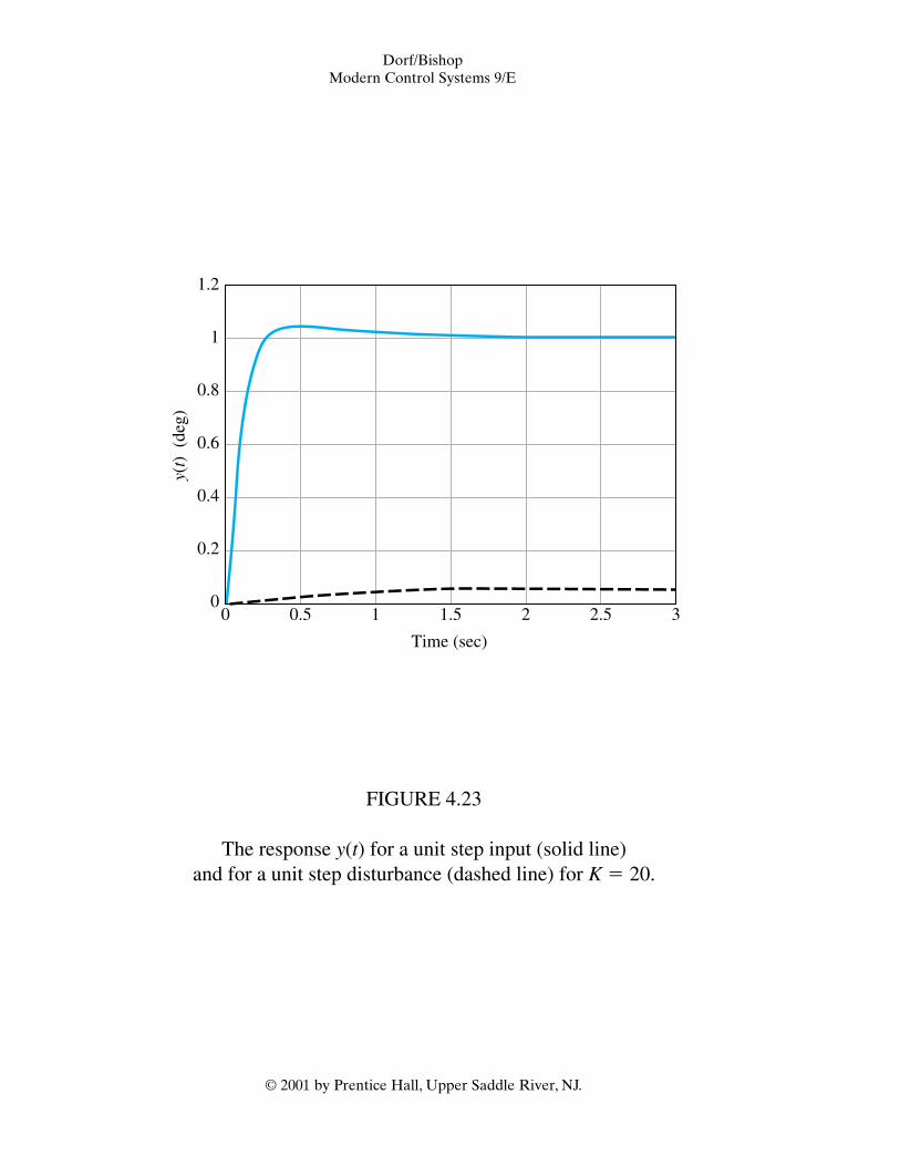
Magnitude of sensitivity vs. frequency
Frequency (rad/s)
Mag
nitu
de o
f se
nsiti
vity
0.60
0.65
0.70
0.75
0.80
0.85
0.90
0.95
1.00
1.05
1.10
10�1 100 101 102
FIGURE 4.26
The magnitude of the sensitivity of the closed-loop system for the Mars rover vehicle.
Dorf/BishopModern Control Systems 9/E
© 2001 by Prentice Hall, Upper Saddle River, NJ.

�
� �
�R(s)
1s(Js + b)
Km
R + L s
V(s)Amplifier Coil Load
Desiredhead
position
Actualposition
ErrorKa
H(s) = 1
DisturbanceD(s)
Y (s)
Sensor
FIGURE 4.32
Control system for disk drive head reader.
Dorf/BishopModern Control Systems 9/E
© 2001 by Prentice Hall, Upper Saddle River, NJ.

�
� �
�R(s)
E(s) 5000G1(s) =
(s + 1000)1
G2(s) =s(s + 20)
Coil Load
Ka
DisturbanceD(s)
Y (s)
FIGURE 4.33
Disk drive head control system with the typical parameters of Table 2.11.
Dorf/BishopModern Control Systems 9/E
© 2001 by Prentice Hall, Upper Saddle River, NJ.

Ka=10;nf=[5000]; df=[1 1000]; sysf=tf(nf,df);ng=[1]; dg=[1 20 0]; sysg=tf(ng,dg);sysa=series(Ka*sysf,sysg);sys=feedback(sysa,[1]);t=[0:0.01:2];step(sys,t);ylabel('y(t)'), xlabel('Time (sec)'), grid
Time (sec)
0 0.2 0.4 0.6 1.0 1.4 1.80.8 1.2 1.6 2.00
0.3
0.2
0.1
0.6
0.5
0.4
1.0
0.7
0.9
0.8
(b)
(a)
Time (sec)
0 0.2 0.4 0.6 1.0 1.4 1.80.8 1.2 1.6 2.00
0.6
0.4
0.2
1.0
1.2
0.8
y(t)
y(t)
Select Ka.
Ka = 10.
Ka = 80.
FIGURE 4.34
Closed-loop response. (a) MATLAB script. (b) Step response for Ka � 10 and Ka � 80.
Dorf/BishopModern Control Systems 9/E
© 2001 by Prentice Hall, Upper Saddle River, NJ.

Ka=80;nf=[5000]; df=[1 1000]; sysf=tf(nf,df);ng=[1]; dg=[1 20 0]; sysg=tf(ng,dg);sys=feedback(sysg,Ka*sysf);sys=–sys;t=[0:0.01:2];step(sys,t);plot(t,y), gridylabel('y(t)'), xlabel('Time (sec)'), grid
(b)
(a)
Time (sec)
0 0.2 0.4 0.6 1.0 1.4 1.80.8 1.2 1.6 2.0-3
-1.5
-2
-2.5
-0.5
0x 10-3
-1
y(t)Select Ka.
Disturbance enterssummer with anegative sign.
Ka = 80.
FIGURE 4.35
Disturbance step response. (a) MATLAB script. (b) Disturbance response for Ka � 80.
Dorf/BishopModern Control Systems 9/E
© 2001 by Prentice Hall, Upper Saddle River, NJ.
�
��
�KR(s) Y(s)
D(s)
1
(s � 1)2
(a)
(b)
1.40
1.00
0.70
00.08
0.50
�0.700 1 2 3 4 5
Time
e(t)
K � 1.0
K � 10
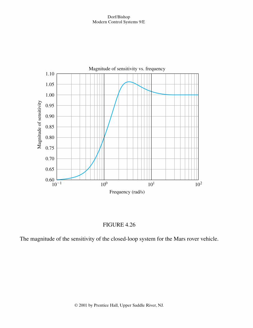
FIGURE 4.36
(a) A single-loop feedback control system. (b) The error response for a unit step disturbance when R(s) � 0.
Dorf/BishopModern Control Systems 9/E
© 2001 by Prentice Hall, Upper Saddle River, NJ.