i

Controller Design for Magnetic Levitation

System

A Thesis Submitted in Partial Fulfillment

Of the Requirements for the Degree Of

MASTER OF TECHNOLOGY

In

Control and Automation

By

Abhishek Nayak

M.Tech

Roll No: 213EE3309

Under the Guidance of

Prof.Bidyadhar Subudhi

Department of Electrical Engineering

National Institute of Technology, Rourkela

Rourkela-769008, Odisha, India

2013-2015

brought to you by COREView metadata, citation and similar papers at core.ac.uk

provided by ethesis@nitr

ii

Dedicated to my family

and my friends

iii

Certificate

This is to certify that the work in the thesis entitled “Controller Design for Magnetic

Levitation System” by Abhishek Nayak is a record of an original research work carried out

by him under my supervision and guidance in partial fulfillment of the requirements for the

award of the degree of Master of Technology with the specialization of Control &

Automation in the department of Electrical Engineering, National Institute of Technology

Rourkela. Neither this thesis nor any part of it has been submitted for any degree or academic

award elsewhere.

Place: NIT Rourkela Prof. Bidyadhar Subudhi

Date: May 2015 Dept. of Electrical Engineering

NIT Rourkela

Department of Electrical Engineering

National Institute of Technology Rourkela

Rourkela-769008, Odisha, India.

iv

ACKNOWLEDGEMENTS

I am grateful to numerous local and global peers who have contributed towards shaping

this thesis. At the outset, I would like to express my sincere thanks to Prof. Bidyadhar

Subudhi for his advice during my thesis work. As my supervisor, he has constantly

encouraged me to remain focused on achieving my goal. His observations and comments

helped me to establish the overall direction of the research and to move forward with

investigation in depth. He has helped me greatly and been a source of knowledge.

I am really thankful to my all friends and especially Abhilash, Manas, Deepthi ,Pavan,

Sudipta, Upasana, Karmila and Debasis. My sincere thanks to everyone who has provided me

with kind words, a welcome ear, new ideas, useful criticism or their invaluable time, for

which I am truly indebted.

I must acknowledge the academic resources that I have got from NIT Rourkela. I would

like to thank administrative and technical staff members of the Department who have been

kind enough to advise and help in their respective roles.

Last, but not the least, I would like to dedicate this thesis to my family, for their love,

patience, and understanding.

Abhishek Nayak

213EE3309

v

Contents CHAPTER 1 .............................................................................................................................................. 1

INTRODUCTION ....................................................................................................................................... 1

1.1 INTRODUCTION .................................................................................................................. 2

1.2 HISTORY OF EVOLUTION ................................................................................................. 2

1.3 TYPES OF MAGNETIC MATERIAL ................................................................................... 3

1.3.1 Ferromagnetic material: .................................................................................................. 3

1.3.2 Anti Ferromagnetic material: .......................................................................................... 3

1.3.3 Diamagnetic material: ..................................................................................................... 3

1.3.4 Paramagnetism: ............................................................................................................... 3

1.3.5 Ferrimagnetism: .............................................................................................................. 4

1.4 MAGNETIC FIELD BASICS ................................................................................................ 4

1.5 MAGNETIC LEVITATION CONCEPT ............................................................................... 5

1.6 TYPES OF MAGNETIC LEVITATION ............................................................................... 5

1.7 APPLICATION OF MAGNETIC LEVITATION ................................................................. 6

1.7.1) Magnetic Levitation train: ............................................................................................... 6

1.7.2) Magnetic Bearing: ........................................................................................................... 7

1.7.3) Launching Rocket: .......................................................................................................... 7

1.7.4) Electromagnetic Aircraft launch system: ........................................................................ 7

1.7.5) MagLev wind turbine: ..................................................................................................... 8

1.7.6) MagLev Microrobot ........................................................................................................ 8

1.8 SCOPE OF WORK ................................................................................................................. 9

1.9 MOTIVATION ....................................................................................................................... 9

1.10 LITERATURE REVIEW ..................................................................................................... 10

1.11 OBJECTIVE ......................................................................................................................... 11

1.12 THESIS ORGANISATION .................................................................................................. 11

1.13 CHAPTER SUMMARY ....................................................................................................... 11

CHAPTER 2 ............................................................................................................................................ 12

SYSTEM DESCRIPTION AND MODELING................................................................................................ 12

2.1 INTRODUCTION ................................................................................................................ 13

2.2 FEEDBACK MAGNETIC LEVITATION SETUP ............................................................. 13

2.3 SET OF EQUIPMENT ......................................................................................................... 14

2.4 BLOCK DIAGRAM ............................................................................................................. 15

vi

2.5 MODELING OF MAGLEV SYSTEM ................................................................................ 15

2.6 CHAPTER SUMMARY ....................................................................................................... 21

CHAPTER 3 ............................................................................................................................................ 22

CONTROLLER DESIGN FOR MAGNETIC LEVITATION SYSTEM ............................................................... 22

3.1 INTRODUCTION: ............................................................................................................... 23

3.2 CONTROLLER DESIGN..................................................................................................... 23

3.2.1: Adaptive backstepping controller: ...................................................................................... 23

3.2.2: Nesic Backstepping on Euler approximate model of MagLev system ......................... 29

3.5 CHAPTER SUMMARY ....................................................................................................... 36

CHAPTER 4 ............................................................................................................................................ 37

SIMULATION AND RESULTS .................................................................................................................. 37

4.1 INTRODUCTION ..................................................................................................................... 38

4.2 SIMULATION OF ADATIVE BACKSTEPPING CONTROLLER ON MAGLEV

SYSTEM ........................................................................................................................................... 38

4.3 SIMULATION OF NESIC BACKSTEPPING CONTROLLER ON MAGLEV SYSTEM ....................... 40

4.4 SIMULATION OF MAGLEV SYSTEM WITH 2DOF PID CONTROLLER .................... 42

4.5 COMPARISION OF THREE CONTROLLERS.................................................................. 43

4.6 EXPERIMENTAL RESULT OF 2DOF CONTROLLER ................................................... 45

4.6.1: 2DOF PID with P1 values: .................................................................................................. 46

4.6.2: Comparison of 2DOF PID with 1DOF PID in experimental setup .................................... 46

4.7 SUMMARY OF CHAPTER ................................................................................................. 47

CHAPTER 5 ............................................................................................................................................ 48

CONCLUSION AND SUGGETION OF FUTURE WORK ............................................................................. 48

5.1 CONCLUSION ..................................................................................................................... 49

5.2 FUTURE WORK .................................................................................................................. 49

Reference .............................................................................................................................................. 50

i

Magnetic Levitation is a method by which an object is suspended in air by means of magnetic

force. Earnshaw stated that static arrangements of magnet cannot levitate a body. The

exception comes in case of diamagnetic and superconducting materials and by controlling

magnetic field by control method. Diamagnetic materials or superconducting materials when

placed in magnetic field produce magnetic field in opposite direction.

Here the problem of controlling the magnetic field by control method is taken up to levitate a

metal hollow sphere. The control problem is to supply controlled current to coil such that the

magnetic force on the levitated body and gravitational force acting on it are exactly equal.

Thus the magnetic levitation system is inherently unstable without any control action. It is

desirable to not only levitate the object but also at desired position or continuously track a

desired path.

Here a linear and two nonlinear controllers are designed for magnetic levitation system. First

a robust adaptive backstepping controller is designed for the system and simulated. The

simulation results shows tracking error less than 0.0001m. The immeasurable state present is

estimated by Kreisselmeier filter. The Kreisselmeier filter is a nonlinear estimator as well as

preserves the output feedback form. However the control output is too high. To counteract

the above problem Nesic backstepping controller is designed for the system by taking Euler

approximate model of the system. The controller output is well within the range of 0.5~1

voltage. The reference tracking is also verified in simulation and the tracking error comes in

range of 0.00015m. A linear controller is also designed for MagLev system as the region of

operation of magnetic levitation setup is too small. A two degree freedom (2DOF) PID

controller is designed satisfying a desired characteristics equation. The controller parameters

are obtained by pole placement technique. The 2DOF PID controller is simulated and

experimentally validated and it is seen that better result are obtained in 2DOF PID than

1DOF PID controller.

ii

List of Figures

1.1 Current carrying wire exerting magnetic field at point Pg 4

1.2 Magnetic force exert by solenoid at a point Pg 4

1.3: Two different models of MagLev train concepts. Pg 6

1.4: Magnetic bearing with controller and position sensing sensor. Pg 7

1.5: Marshall Space Flight Center at Huntsvhill, Alabama. Track of 15 meter long. Pg 7

1.6: U.S Navy model MagLev catapult. Pg 7

1.7: MagLev wind turbine as proposed by Guangzhou Energy Research Institute. Pg 8

1.8: Khamesee MagLev microrobot. Pg 8

2.1: Magnetic Levitation mechanical unit. Pg 14

2.2: Analogue control interface unit. Pg 14

2.3: Block diagram of Maglev system with controller. Pg 15

2.4: Schematic diagram of closed loop system Pg 15

2.6: Conservative magnetic field system Pg

2.5: Net force acting on metallic ball Pg 16

3.1: Schematic diagram of closed system with adaptive backstepping controller Pg 24

3.2: Estimation of state 2x in closed loop for different k with step reference for different k

Pg 26

3.3: Schematic diagram of Backstepping on Euler approximate model Pg 27

3.4: Schematic PID controller Pg 32

3.5: Schematic diagram of 2DOF controller Pg 33

3.6: Schematic diagram of linear model Pg 33

3.7: Schematic diagram of 2DOF PID Pg 33

iii

3.8(a): Bode plot of sensitivity function. Pg 35

3.8(b): Bode plot of complementary sensitivity function. The maximum value is 2.1db

Pg 35

4.1: Showing tracking response with step as reference for different1 2&c c values Pg 38

4.2: Simulation plot for different mass of ball Pg 39

4.3: Simulation plot of MagLev system with sqaure wave reference Pg 39

4.4: Simulation plot of MagLev system with Sine wave reference Pg 40

4.5: Control signal values for step reference Pg 40

4.6: Simulation plot for step reference with different 1 2&c c values Pg 41

4.7: Plot of error between auxiliary control and stabilizing function Pg 41

4.8: Simulation result for square wave reference Pg 41

4.9: Simulation result for Sine wave as reference Pg 42

4.10: Simulation results of MagLev model with different value of 1P Pg 42

4.11: Simulation result of MagLev system with square wave reference Pg 43

4.12: Simulation result of MagLev system with Sine wave reference Pg 43

4.13: Plot of all controller for square wave reference Pg 44

4.14: Plot of all controller for sine wave reference Pg 44

4.15: Plot of all controller control values Pg 45

4.16: Experimental setup of Mag-Lev system Pg 45

4.17: 2DOF PID with different P1 values 0,-1, 1. Pg 46

4.18: Comparison of 2DOF PID and 1DOF PID Pg 46

iv

List of tables

Table 4.6.1: Comparison of experimental results of 2DOF PID and 1DOF PID. Pg.45

Table 4.6.1: Comparison of experimental results of 2DOF PID and 1DOF PID. Pg.47

v

List of Acronym

1. MagLev : Magnetic Levitation

2. IR : Infra Red

3. DOF : Degree Of Freedom

4. CLF : Control Lypunov Function

5. SPA : Semiglobally Practically Asymptotic

1

CHAPTER 1

INTRODUCTION

INTRODUCTION

HISTORY OF EVOLUTION

TYPES OF MAGNETIC MATERIAL

MAGNETIC FIELD BASIC

MAGNETIC LEVITATION CONCEPT

APPLICATION OF MAGNETIC LEVITATION

SCOPE OF WORK

MOTIVATION

LITERATURE REVIEW

OBJECTIVE

THESIS ORGANISATION

CHAPTER ORGANISATION

CHAPTER SUMMARY

2

1.1 INTRODUCTION

Magnetic Levitation is a method by which an object is suspended in the air with no

support other than the magnetic field. Difficulty in stably levitating an object by using

inverse square law was studied by Samuel Earnshaw in 1842 [1]. Earnshaw‟s

Theorem states that a point charge cannot have stable equilibrium position when a

static force is applied following the inverse square law. This theorem is also

applicable to the magnetic force of the permanent magnet. Werner Braunbeck

extended the analysis to uncharged dielectric bodies in electrostatic fields and

magnetic bodies in magnetostatic fields in 1939. The same analysis was also done by

Papas (1977). It was observed that for diamagnetic material, super conducting body

and conducting body with eddy current induced on them can have stable equilibrium

point.

1.2 HISTORY OF EVOLUTION

Work on using permanent magnet can be date back to 1890. Application to shafts of

wattmeter or spindles was carried out by S.Evershed (1900) [2];Faus (1943) and

Ferranti (1947) [3,4]. The first demonstration of levitating bodies by using

superconducting effect is studied by Arkadiev (1945, 1947) [5,6]. Kemper (1937,

1938) suspended an electromagnet using active control [7]. Holmes in 1937

developed controlled ac supply electromagnet to suspend rotor of ultra-high using

speed centrifuges and Beams in 1937 [9][10] developed electromagnetic suspension

system using control ac electromagnet. Magnetically levitated gyroscope was

demonstrated by Simon (1953) [11] and levitating a superconducting sphere over

different arrangement of electromagnets was demonstrated by Culver and Davis

(1957) [12][13]. Levitation of a vehicle over a superconducting rail was proposed by

James R. Powell (1963).James R. Powell and Gordon T. Danby (1966) proposed

attaching a super conductor to base of a vehicle and levitate it over a conducting rail

[14]. The duo were granted U.S patent for their magnetic levitation train model. There

were several proposal of using transportation mode by using magnetic levitation was

proposed in 1960s and 1970s. Japan and Germany are two countries which actively

took research on mass transportation using magnetic levitation. Germany model

basically suspends the train on the underside way of guideway using attraction

between the electromagnet on the train and the rail plate on the underside of the

carriage. However in Japanese model the train surrounded by guideway wall and

3

track, where the center of guideway is above the superconductor situated under the

train. In April 2004 Shanghai Transrapid system began commercial operational which

uses the German method and in March 2005, HSST “Linimo” started commercial

operational.

1.3 TYPES OF MAGNETIC MATERIAL

Classification is made depending on the different type of material behavior towards

the magnetic field.

1.3.1 Ferromagnetic material:

These are the materials in which magnetic moments of atoms or molecules

align in a regular pattern with all moments pointing in same direction in the

magnetic field.

Example: Iron, Nickel, Cobalt, Steel etc.

1.3.2 Anti Ferromagnetic material:

These materials have magnetic moments of atom or molecules align in a

regular pattern with all moments pointing in the opposite direction to

neighboring moments.

Example: transition metal compounds especially oxides, Hematite, Chromium,

Iron Manganese etc.

1.3.3 Diamagnetic material:

Diamagnetic materials, when applied to magnetic field create a field in the

opposite direction to the applied field. Diamagnetism is a quantum mechanical

effect that occurs in all materials. When only contribution of magnetism is

considered then it is called as diamagnetic material.

Example: Copper, Carbon Graphite, Lead etc.

1.3.4 Paramagnetism:

Paramagnetic materials are attracted towards the magnetic field and magnetic

fields induced are in direction of magnetic field when applied with magnetic

field are. The magnetic property is lost when magnetic field is removed.

Example: Sodium, Manganese, Lithium etc.

4

1.3.5 Ferrimagnetism:

Ferrimagnetic materials have magnetic moments opposite as in

antiferromagnetism but the opposing moments are unequal in ferromagnetic

materials.

Example: Yttrium iron garnet, Cubic ferittes composed of iron oxide etc.

1.4 MAGNETIC FIELD BASICS

The magnetic field at a certain point can be given by Biot Savart law (1820). The law

state that a current carrying element „ dl ‟ carrying current „ i ‟ contributes magnetic

field „ B ‟ at a point „ P ‟ which is normal to plane of „ dl ‟ with vector „ r ‟ is given by

P

i

dB

dl

r

Figure 1.1 Current carrying wire exerting magnetic field at point P

0

2

i dl sin

4dB

r

Where

0 is permeability constant in free space

i is current in the element

B is magnetic field

dl small section of wire carrying current

r vector from the element to the point „P‟

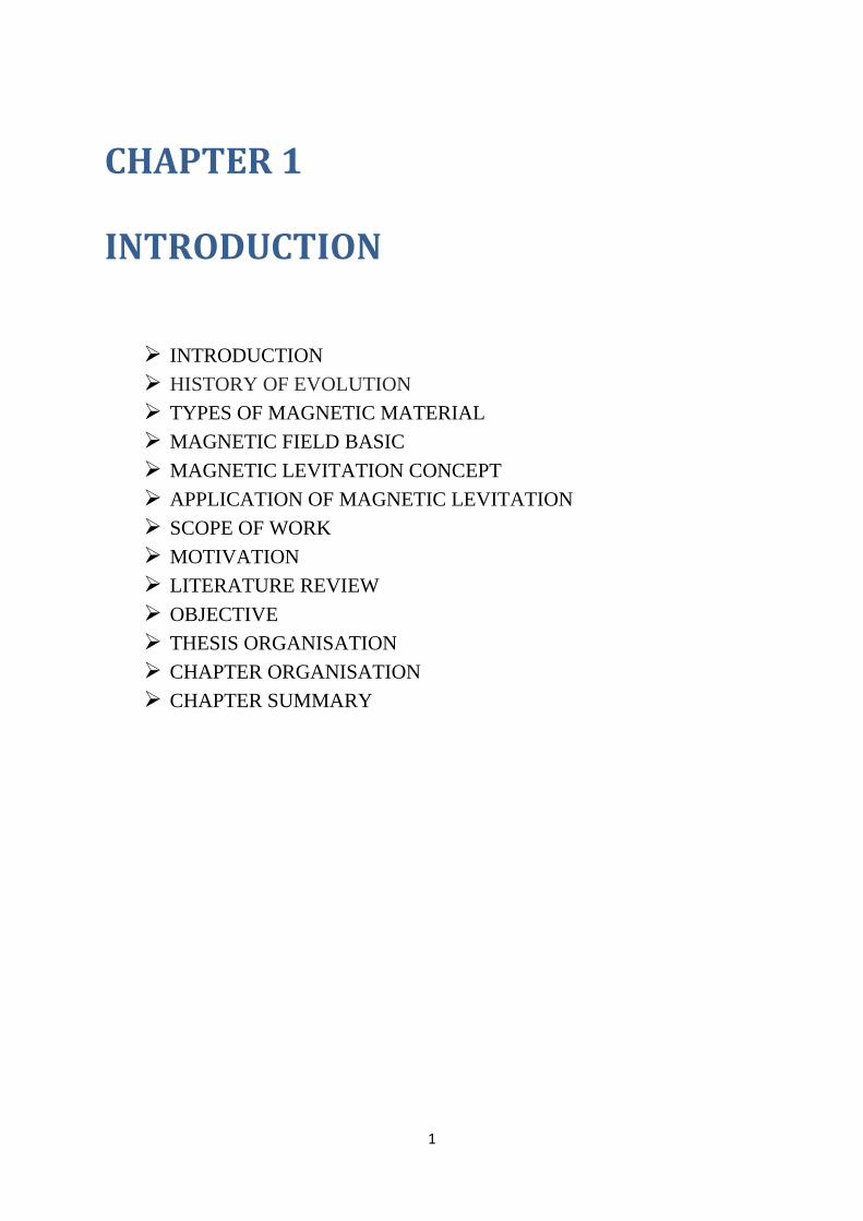
Whereas in magnetic levitation system electromagnetic coil are used to produce the

magnetic field. Magnetic field inside solenoid is given by

5

R

r

P

x

X

Figure 1.2 Magnetic force exert by solenoid at appoint P

2 2 2 2

0

2 2 2 2ln ln

2( )

in R X R R X RB X x

R r r x r r x r

Where

B, 0 , i stands same as above

n number of turn in per unit length in solenoid

,R r outer and inner radii of solenoid respectively

,X x distance between the ends of solenoid to point where the magnetic

field is measured.

However we use directly energy balance concept to find out the force acting on the

levitating body [26]. The magnetic force is derived latter on.

1.5 MAGNETIC LEVITATION CONCEPT

Magnetic levitation is an electromechanical coupling concept [35]. The magnetic field is

created by electromagnet coil which is electrical part attracts the magnetizable material

or object. The magnetic force is controlled by controlling the current in the coil. When

the object moves to close the magnet the current in the coil is decreased and vice versa.

1.6 TYPES OF MAGNETIC LEVITATION

Magnetic Levitation can be classified according to magnetism as

a) Levitation by attraction:

This works on the principle that when two magnets are placed end to end with

opposite pole facing each other.

b) Levitation by repulsion

This works on the principle that when two magnets are place end to end with same

pole facing each other.

6

Magnetic Levitation can be classified according to principle by which levitation is

made as [41]

i) Levitation by repulsive force between magnets of fixed strengths

ii) Levitation by magnetic field on diamagnetic materials

iii) Levitation by superconducting surface

iv) Levitation by eddy current induced on conducting surface due to magnetic

field

v) Levitation by force acting on current carrying conductor in magnetic field

vi) Levitation by controlled DC or AC supply to electromagnetic coil by control

algorithm

vii) Mixed systems where system are materials where some place the

permeability is less than 1 and in some place more than 1.

1.7 APPLICATION OF MAGNETIC LEVITATION

Magnetic levitation systems have advantages of friction less movement, isolation of

environment and high precision. Some of the applications of magnetic levitation are

stated below:

1.7.1) Magnetic Levitation train:

Magnetic Levitation (MagLev) train has been the most important usages of

magnetic levitation technology. The train moves along the guide way with the

help of magnetic field which helps the train to levitate and propel. In March 2004

first MagLev commercially implemented was Sanghai‟s Transrapid system which

uses German model and in April 2005 Japan implemented its own HSST

„Limino‟.at relatively slow speed than Shanghai one. The fastest train „Lo‟ Japan

is the fastest train till recorded of speed 603km/hr.

Figure 1.3 Two different model of MagLev train concepts [36].

7

1.7.2) Magnetic Bearing:

Magnetic bearing use rotor to levitate and rotate with magnetic flux interaction

from stator mounted electromagnet. Since no contact thus no friction, no drag and

no wear and tear of parts. Magnetic bearing are used in flywheel as energy storage

device, as blood pump, micro positioning system and semiconductor industries.

Figure 1.4 Magnetic bearing with controller and position sensing sensor [37]

1.7.3) Launching Rocket:

NASA‟s Marshall Space Flight Center at Huntsvhill, Alabama has developed a

track to magnetically levitate a space craft and give initial velocity to reach escape

velocity of earth. The project is to make space transportation with less cost. The

space craft will be able to have 964km/hr when launched from the track without

having any fuel consumption.

Figure 1.5 Marshall Space Flight Center at Huntsvhill, Alabama. track of 15 meter long [38].

1.7.4) Electromagnetic Aircraft launch system:

Electromagnetic Aircraft launch system uses magnetically levitated based catapult

to launch aircraft in aircraft carrier. This system achieved better acceleration than

conventional linear motor as well the stress on air frame of aircraft is also less.

8

Figure 1.6 U.S Navy model MagLev catapult [39]

1.7.5) MagLev wind turbine:

Guangzhou Energy Research Institute researcher have estimated that magnetically

levitated wind turbine can as much 20% more efficient than traditional wind

turbine. The proposal is given for colossal wind turbine with vertical blades and

supported by neodymium magnets. Since the efficiency is more thus area required

to generate same power is much less here than traditional wind turbine.

Figure 1.7 MagLev wind turbine as proposed by Guangzhou Energy Research Institute [17]

1.7.6) MagLev Microrobot

MagLev microrobots are being studied in University of Waterloo for possible

application in hazardous environment, for dust free application and micro

assembly of hybrid microsystems. Behrad Khamesee have presented a paper on it

[42].

9

Figure 1.8 Khamesee MagLev microrobot [40]

There are many more application areas which are continuously being explored.

MagLev is a new technology which has been an actively research area.

1.8 SCOPE OF WORK

Magnetic Levitation is an open loop unstable system. The whole system is an

elctromechanical coupled system. Thus modeling of the system is difficult task which

is first carried out. Since the system is nonlinear and unstable thus control problem is

challenging. Nonlinear and linear control techniques are derived to satisfy certain set

of performance. The control techniques are then simulated and applied in

experimental setup to verify their effectiveness.

1.9 MOTIVATION

MagLev is a non-contact technology thus finds application in high speed

transportation system as there is no friction, since there is no friction it can applied to

high precision system, also absence of friction gives way to no wear and tear of

moving parts which results in high longevity e.g MagLev bearing and also no dust

pollution thus creates a clean environment where very high purity is required e.g

semi-conductor industry. MagLev also creates environment separation thus one can

operate from one environment to another environment eg. Heart pump, in medical

industry and in hazardous places. Thus MagLev can be said to be a future technology

and it has a vast area of application to be uncovered. All this applicability comes at

the cost of either a good design of superconducting magnet (which is inherently

stable) or good controller design because fundamentally the levitation by

electromagnet is unstable. Here we consider for designing a controller which

10

stabilizes the levitated object through continues monitoring of position and feed

backing it. The MagLev system is a nonlinear and open loop unstable system. Thus it

provides an exciting opportunity for controller designer to explore different control

algorithm for the system.

1.10 LITERATURE REVIEW

In recent years there has been active research in control of both attractive and

repulsive type magnetic levitation. Huang(2000) proposed adaptive backstepping

controller for repulsive magnetic force of a MIMO system. The adaptive backstepping

controller proposed for decoupling nonlinearities and eliminating uncertainties[3].

Yang et al (2000) controller design method was to stabilizing the position error of

levitated object by a PI controller and adaptive robust nonlinear controller

(backstepping method) is designed to attenuate the effects of parameter uncertainties,

so that a small velocity error is ensured[4]. Lepetic et al(2001) applied a method of

fuzzy predictive functional control to MagLev system. First a lead compensator was

designed to stabilize the system then fuzzy controller is applied based on TS rule [5].

Nesic et al proposed a method to implement backstepping in realtime where plant is in

continuous form and the controller is implemented though computer or digitally, here

an Euler approximate model of system is considered and controller is designed

accordingly [18]. Dan Cho et al (1993) Jalili-Kharaajoo (2003, 2004), and Fallaha et

al. (2005) proposed sliding mode controllers (SMC) for magnetic levitation system [6,

7, 8]. In all previous case the velocity state is obtained by psodifferentiation of

position state. Z-J Yang et al (2008) consider K-filter approach to observer the

unmeasured state and apply backstepping to the new dynamics. The velocity state is

estimated by Kreisselmeier filter as it is not measurable [14, 15]. Yang et al. (2011)

investigate controller via a disturbance observer based control (DOBC) approach to

address the mismatched uncertainties in system. The author also proposed disturbance

compensation based on estimated disturbance. The disturbance estimated are

considered as lumped disturbance and the plant considered is a linearized plant [9].

Ghosh et al (2014) designed by using 2-DOF PID controller, the PID parameters are

obtained by using pole placement techniques [10]. .Beltran-Cabajal et al (2015)

presented an application of MagLev in a mass spring damper system. The tracking of

reference is achieved by output feedback controller. The system states are also

estimated by an estimator [19].

11

Thus a brief conclusion is achieved as there is active research going on adaptive,

robust control and linear control on Magnetic Levitation system by linearizing plant

or taking direct nonlinear plant. Thus MagLev provides a test bed to test different type

controllers.

1.11 OBJECTIVE

The objective of the work can be directed to design controller considering the linear

model as well as nonlinear model. The controller designed is validated by simulating

and implementing on real time system.

1.12 THESIS ORGANISATION

The thesis is organized into five chapters with each chapters has its own subsection.

The chapters are briefly described as below

Chapter 1: This chapter briefly introduces the magnetic levitation technology,

history of development, some application, and motivation of taking the

project, literature review of some previous works and objective of

work.

Chapter 2: This chapter describes the Magnetic Levitation setup on which the

controller is tested and mathematical modeling of the system.

Chapter 3: In this chapter controller is designed based on the model achieved.

Chapter 4: In this chapter the controller designed is simulated and the result are

discussed. The experiment validation of proposed controller is also

carried out.

Chapter 5 Conclusion part and future work are discussed in this chapter.

1.13 CHAPTER SUMMARY

This chapter briefly describes the MagLev system working principle, gives a brief

history of how the MagLev system explored from time to time, some application of

the MagLev system. The chapter also describes the motivation of author to take the

project and also the objective which the author set to achieve.

12

CHAPTER 2

SYSTEM DESCRIPTION AND

MODELING

INTRODUCTION

FEEDBACK MAGNETIC LEVITATION SETUP

SET OF EQUIPMENTS

BLOCK DIAGRAM

MODELING OF SYSTEM

CHAPTER SUMMARY

13

2.1 INTRODUCTION

This chapter gives an idea of the magnetic levitation system provided by “Feedback”

company and other set of equipment required to perform the experiment. The later

part of chapter deals with modeling of a magnetic levitation system. In modeling a

linear and nonlinear model of the MagLev system is derived. Here magnetic force

causing the levitation is also derived.

2.2 FEEDBACK MAGNETIC LEVITATION SETUP

Magnetic levitation setup plant consists of three important parts

a) Electromagnetic coil

b) Infrared light sensors

c) Metal object

d) Analogue and Digital interface

e) Controller from computer

a) Electromagnetic coil: The electromagnetic coils gives necessary magnetic field

when current is passed through it. The produced field interacts with the metallic

object to produce the necessary lifting force. A heat sink is provide to regulate

the temperature of coil after prolong current supply is provided.

b) Infrared light Sensor: There are two parts in IR sensor. One is the transmitter of

IR light and other is receiver of IR light. Base on the amount of light fall on the

receiver voltage is produced. When object is in levitation position then the

some part of the lights are blocked and correspondingly voltage is produced.

The amount of the voltage produced gives the position of the object.

c) Metal Object: Here a hollow metallic ball is considered as object. The weight

of the ball is around 20 grams.

d) Analogue and Digital interface: The Maglev plant is the interface with a

computer via Analogue and Digital interface as the plant is in continuous time

domain whereas the computer works in the digital domain. Thus to couple both

an interface is needed. Sensor output is feed to analogue to digital converter pin

and the control input from the controller in computer feed to digital to analogue

converter pin.

e) Controller: The maglev plant is open loop unstable. Thus to perform levitation

a controller is needed. The necessary controller is designed in MATLAB or

14

Simulink and connected to MagLev system via Advantech PCI1711 card. The

control output is bounded to be within +5V and -5V [27].

Figure 2.1 Magnetic Levitation mechanical unit

Figure 2.2 Analogue control interface unit

2.3 SET OF EQUIPMENT

Set of equipment required for experiment are as follows [27]

i) Feedback Magnetic Levitation setup

ii) Hollow metallic ball

iii) Feedback Analogue control interface

iv) PC with Windows 2000 or Window XP

v) MATLAB V7.3(R2006b) or later version

vi) MATLAB Toolbox required:

Analogue to digital interface

Digital to analogue interface

15

Real Time Workshop with real time target

System Identification tool box

Control tool box

vii) Advantech PCI17111 card

viii) Installation software

2.4 BLOCK DIAGRAM

The block diagram of whole system is given as

MagLev

PlantController

RefBall position

Current to

magnetic coil

Computer Unit

Feedback by IR sensor

External disturbance

Sensor noise

Figure 2.3 Block diagram of Maglev system with controller

Figure 2.4 Schematic diagram of closed loop system

2.5 MODELING OF MAGLEV SYSTEM

The metallic ball dynamics under equilibrium position, when applied with

electromagnetic field is given by Newton law as

16

. . em x m g f (2.1)

Where,

m = mass of the ball

x = position of ball

g = gravitational acceleration

ef = magnetic force

The magnetic force is derived by given J.L Kirtley Jr [26].

There are basically two approach of finding the magnetic force i.e Thermodynamic

argument (conservation of energy approach) and Field method (Maxwell's field

Tensor) method.

Here energy approach is used to find the electromagnetic force. The magnetic field

system is considered as conservative system i.e input energy to the system is same as

output energy of the system. In the magnetic field system the input is electrical and

output is mechanical i.e movement of the object. There no loss of energy in the form

of heat or friction.

Magnetic field

system

V

+

-

x

Figure 2.6 Conservative magnetic field system

Since there is no energy loss the energy stored in the magnetic field system. The

energy stored in the system depends on two states only i.e flux ( ) or current ( i )

and mechanical position ( x ) as seen from Figure 2.6.

Metallic

ball

m.g

ef

Figure 2.5 Net force acting on metallic ball

ef

17

Electrical power input the conservative system is

. .e

dP v i i

dt

Mechanical power out of system can be written as

m e

dxP f

dt

The difference of two is rate of change of energy stored in system

me m

dWP P

dt

e

mdW d dxi f

dt dt dt

(2.2)

For taking the system from one sate to another, we may write

( ) ( ) . .

b

m m e

a

W a W b i d f dx

where

two states are ( , )

( , )

a a

b b

a x

b x

Now the energy stored the system can be written in term of two state variables i.e

& x as

m mm

W WdW d dx

x

(2.3)

Comparing (2.2) and (2.3) we get

me

Wf

x

(2.4)

mWi

(2.5)

Now for multiple electrical terminals or multiple mechanical terminals (2.2) can be

written as

18

.m k k e

k

dW i d f dx

. .m edW i d f dx (2.6)

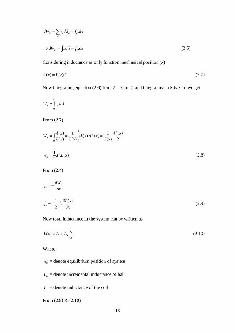
Considering inductance as only function mechanical position (x)

( ) ( ).x L x i (2.7)

Now integrating equation (2.6) from = 0 to and integral over dx is zero we get

0

.m kW i d

From (2.7)

2

0 0

( ) 1 1 ( )( ). ( )

( ) ( ) ( ) 2m

x xW x d x

L x L x L x

21. . ( )

2mW i L x (2.8)

From (2.4)

me

dWf

dx

21 ( ). .

2e

L xf i

x

(2.9)

Now total inductance in the system can be written as

01 0( )

xL x L L

x (2.10)

Where

0x = denote equilibrium position of system

0L = denote incremental inductance of ball

1L = denote inductance of the coil

From (2.9) & (2.10)

19

2 2

0 0. 2 2

1

2e

i if L x k

x x (2.11)

Where k is constant which depends on system

Now plant dynamics can be written from (2.1) & (2.11) as

2

1 2

ix g k

x (2.12)

Linearization (2.12) around equilibrium point 0 0,x i

( , )x F i x

0 0 0 0( , ) ( , )| |i x i x

F Fx x di dx

i x

0 0 0 0( , ) ( , )| |e ei x i x

f fdi dx

i x

0 01 2 3

0 0

2. .i i

k i xx x

(2.13)

at equilibrium point from (2.12)

2

1 2

0

0 oig kx

2

01 2

0

ig k

x (2.14)

From (2.13) and (2.14)

0 0

2 2g g

x i xi x

Taking 0

2i

gK

i and

0

2x

gK

x

. .i xx K i K x

Taking Laplace transform

2. . .i xs X K I K X

20

2( ) i

x

KXG s

I s K

(2.15)

By substituting equilibrium point as 0 00.8 & 1.5 (0.009 )i A x V m

Transfer function of linearized system around equilibrium point is given as

2

24.525( )

2180G s

s

(2.16)

The Feedback MagLev system provided has internal circuit to make voltage

proportional to current

1.05i V (2.17)

The output from sensor (mx ) is given by

143.48 2.8v mx x (2.18)

Where

mx is actual position in meter, with electromagnet endpoint is considered as 0 meter

The state space model is given as

1 2

2

2 1 2

1

x x

ix g k

x

(2.19)

where

1x is given as position state

2x is given by velocity state

21

2.6 CHAPTER SUMMARY

This chapter describes the overall system. First the hardware setup description is

given by Feedback is discussed. Then the set of equipment is described and block

diagram of the overall system with the controller is shown. Lastly, the mathematical

model of the system is derived.

22

CHAPTER 3

CONTROLLER DESIGN FOR MAGNETIC

LEVITATION SYSTEM

INTRODUCTION

ADAPTIVE BACKSTEPPING CONTROLLER

DISCRETE MODEL BACKSTEPPING CONTROLLER

TWO DEGREE FREEDOM (2DOF) PID

COMPARISION OF THREE CONTROLLERS

EXPERIMENTAL RESULT

CHAPTER SUMMARY

23

3.1 INTRODUCTION: Since MagLev system is an open loop unstable thus controller design is very critical part of

the close system. Since the system is nonlinear, controller design can be carried out by taking

nonlinear model as well as linearized model. Since all the states are not measurable a

nonlinear estimator is also designed. Here three controller are designed

1) Adaptive Backstepping controller.

2) Backstepping on Euler approximate of MagLev system.

3) Two degree freedom (2DOF)PID controller.

3.2 CONTROLLER DESIGN

3.2.1: Adaptive backstepping controller:

Backstepping control design method was by “Krstic, Kanellakopoulos, and

Kokotovic” circa 1990. Backstepping is a non linear controller which can be applied

to nonlinear system having strict feedback form. The control technique is to reduce

the system into subsystem and each system is controlled by an auxiliary control. The

auxiliary control follows the stabilizing function. The stabilizing function forms the

control Lyapunov function. The original control is achieved by stepping backing from

subsystems to last subsystem. Thus the control technique is called backstepping

control.

Let a system is given as

( ) ( )x f x g x (3.1)

u

Where , ,nx u

Note 1n

x

are state of system

u is control input.

Assumptions:

, : nf g D are smooth

(0) 0f

is auxiliary input to (3.1). Stabilizing function is given as ( )x where

(0) 0 . Also a Lyapunov function 1 :V D such that

11( ) ( ) ( ). ( ) ( ) x D

T

a

VV x f x g x x V x

x

24

Where ( ) :aV x D is positive definite function

Now the error dynamics is defined as

Z

Z u

Where „u‟ satisfying 21

2V Z

Thus control input is derived.

Objective of controller: The design objective to stabilize the error dynamic. Error

dynamic state are of two states. 1st is error between the plant output(i.e) Ball position

and reference. 2nd is error between the virtual control and stabilizing function. The

actual control is backstep by virtual control.

Figure 3.1 Schematic diagram of controlsystem with adaptive backstepping controller

Now from system (2.19) 1x is only measurable by position sensor but 2x is not

measurable as an extra sensor to measure accurate velocity may not be cost effective

and differentiation of 1x may give noisy output. So we estimate the 2x by

Kreisselmeier filter [28].

Kreisselmeier Filter is given by:

For a system

25

. ( ) ( , )Tx A x y F y u

1 .Ty e x

Where b

a

are unknown parameters of system.

( 1) ( 1)

1

0( , ) ( ). ( )

p mT

m

F y u y u yI

are the nonlinear terms multiplied with

parameter uncertainties

1[ ,......., ]T

nk k k is chosen such that the matrix 0

TA A k e is Hurwitz.

The observed state will be governed by system

0x A x where ˆx x x

Estimated state is given by

ˆ Tx (3.2)

Filter is

0

0

( )

( , )T T

A ky y

A F y u

(3.3)

Now Kreisselmeier Filter deign for the system (2.19)

2 2ˆe x x is the error between the estimated velocity and the actual velocity.

The filter is constructed such that

2 2x k x where 2 2 2ˆx x x

Now here we estimate 2x as

2 1x A kx (3.4)

Where

2

1k k x g (3.5)

2

2

1

ik

x

(3.6)

The step response for different values of „k‟ in shown in Figure 3.2 .It can be seen that

as „k‟ increases the tracking error decreases but the initial value of 2x increases by a

factor of 10 as k is increased by factor of 10. Thus a oscillatory response is observed

26

in starting in closed loop system with step input. The effect is more prominent in fast

changing reference signal like square wave, sine wave. Thus „k‟ is taken as 10

Figure 3.2 Estimation of state 2x in closed loop for different k with step reference for different k

In system (2) we cannot apply backstepping as 2x is not measurable

Thus new system is formed as to which we apply backstepping

1 2x x (3.7)

2

2

1

ik

x

(3.8)

Design of Backstepping controller for MagLev System

The design objective is to regulate 1x to a given set point ry . In the above equations (5) the

1st equation has as virtual control, 2

nd equation i is virtual control Thus our goal is to

stabilize the error co-ordinate as below.

Error co-ordinate

1 1 rZ x y

2 1Z (3.9)

Taking CLF as 1 1

1

2V Z

Finding 1Z and stabilizing function 1

1 1 1 2 rZ kx A AZ y

(3.10)

Taking 1 1a

27

Where 1

aA

ˆa a a

Thus taking first stabilizing control as

1 1 1 1 1 1kx c Z d Z (3.11)

Thus resulting 1Z

1 2 1 1 1 1 rZ AZ c Z d Z Aa y (3.12)

The term - 1 and 1kx cancels the same term in (3.12) 1 1c Z produces CLF to be negative ,

1 1d Z is introduce to give damping as is present. Here 1 1a because an unknown term (

A ) is multiplied with 1 in 1Z expression .The term 1Aa get cancelled in updating law

2AZ is canceled in 2Z which we will get later (3.13).

Now

2 2

2 1 2

1 1

2 2V x x

2Z =

2

1 1 112

1 1 1

ˆˆ

ik x

x x

(3.13)

Here we get control input as i as

2 21 1 1 11 2 2 1 1 1 2 2

1 1

ˆ ˆ ˆ( ( ) ( ) ( ) )ˆ

i x k c Z A kx k k x g AZ d Z ax x a

(3.14)

Where

1 1 11

1

ˆk x ax a

terms are used to cancel the same in (3.13), 2 2c Z is used to

produce negative CLF, 1AZ get canceled while considering 2Z matrix 21

2 2

1

( )d Zx

is

used to produce damping which is produce to counteract term.

28

While placing 1Z 2Z in 2V

We get extra terms of unknown terms

Now

2 2

2

1 2

1 1

2 2V V a A

Finding V such that it is 2 2

1 2x x

Thus tuning law is obtained as

1 1 1a Z

12 1 2 2

1

A Z Z Zx

(3.15)

Substituting 1, i in 1Z , 2Z we get

1 1

1 1

2 112 2 22

11

( ) 1

( )

c d AZ Z

A c d ZZxx

1

11

1

0

0

Aa

Z Ax

(3.16)

From the above we note that the 1st matrix is a skew symmetric which is a property of

backstepping controller, 2nd

matrix is error term of 2x and the last term comes as parameter

error terms , from the last term we design the tuning laws as transpose of it.as can be seen

in[28].

Assumption

i) Here we consider for modeling plant the internal inductance 0( )L to 5.518125 mH ,

the initial position 0( )x to be 0.009m . Thus „A‟ (the unknown parameter) in model comes to

be 31.241578125 10 (for mass ( )M =20g).

0 k

AM

where 0 00

2

L xk

ii) The initial values of ˆˆ &a A are taken as 1000 and 31 10 , considering „A‟ to be in

310 range.

Now taking 1 1000c , 2 2000c , 1 2 1 22, 2, 100, 100d d

29

The constants value are taken in the guide lines as 1c less than 2c because 1c represents

rate of decrease of 1Z (tracking error)and 2c represent rate of decrease of 2Z (auxiliary

controller and stabilizing function error), thus for a fast convergence of auxiliary control with

stabilizing function the auxiliary controller will control the tracking error. It is seen that with

less 1c value initial error is more. However with more value of 1c the control action is

increased. Thus a tradeoff is made by choosing 1 1000c , 2 2000c , 1d , 2d are taken

small so that the control action will be less. For „k‟ value should be large as it decides the rate

of convergence of but too large will allow more band width thus filter output becomes

noisy. Thus value of 10k is taken. The values of 1 2, are taken as 100 each as the initial

values of tuning parameter values are taken too close to the actual values. Taking high values

of 1 2, will increase computational burden and thus increases the response time.

3.2.2: Backstepping on Euler approximate model of MagLev system

Backstepping controller technique has very well understood when the plant and the

controller both are in continuous form. However for digital implementation of

controller the either of two approach can be taken. One is designing controller for

continuous time and implementing it directly using sample and hold. A shortcoming

of the direct implementation of controller is ignoring the sampling completely. Where

as the other method is to design a controller considering the sampling time by using

discrete time model of system. However obtaining exact discrete model in strict

feedback form is unrealistic as the plant is in continuous form. Thus sampling

destroys strict feedback structure which is necessary for backstepping. Euler

approximate model however preserves the .strict feedback structure. Dragan.Nesic

proposed a backstepping controller using an Euler approximate model for a nonlinear

system[33].

Let a system given as

( ) ( )x f x g x

u

(3.17)

Euler approximate model

( 1) ( ) ( ( ( )) ( ( )) ( ))x k x k T f x k g x k k (3.18)

( 1) ( ) ( )k k Tu k (3.19)

30

Where

T is sampling time

Now considering the Theorem given by D.Nesic [33].

Theorem: Consider the Euler approximate model (3.18). Suppose that there exist

ˆ 0T and a pair ( , )T TW that is defined for all ˆ(0, )T T and that is a SPA stabilizing

pair for the subsystem (3.19) ,with regarded as its control. Moreover suppose

that the pair ( , )T TW

has the following properties:

i) T and

TW are continuously differentiable for any ˆ(0, );T T

ii) there exist K such that

( ) ( )T x x

iii) for any 0 there exist a pair of strictly positive numbers ( , )T M such that

for all 0,T T and x we have

,T TWmax M

x x

Then there exists a SPA stabilizing pair ,T Tu V for the Euler model (3.18),(3.19). In

particular, we take:

( ) ( ( )) T TT T

Wu x c x

T T

(3.20)

where 0c is arbitrary,

( ( )) ( )T T Tx T f g x

( )( )

( ( ( ) ( ) ) ( ) ( )

TT

TT

TT

Wx

WW

T x T f x d x g x xx

(3.21)

( ( )) ( ( ))T T T TW W x T f g W T f g (3.22)

And 21( ) ( ) ( ( ))

2T T TV x W x (3.23)

Thus control law is formulated as above from Theorem.

31

Objective of Controller: For control law obtained above the control output are too

high, so practical implementation is bit difficult as the actuator input are limited. Thus

here a controller is designed whose control outputs are bounded. The controller design

takes into consideration of Euler approximate model.

Figure 3.3 Schematic diagram of Backstepping on Euler approximate model

The stabilizing function ( ) remains same as derived in (3.11),the K-Filter also

remains same as in (3.4),(3.5) and (3.6) and error dynamics also remains same (3.9).

2 2

1 1 1 1

1 1ˆ ˆ[ ( ) ] [ ( ) ]2 2

T r r r rW x T kx A y Ty x T kx A y Ty (3.24)

After solving we get.

2 22 2 2 2 2 2 2 2 2

1 1 1 1

ˆˆ ˆ ˆ ˆ ˆ( ) ( ) ( ) 2 ( ) 2 ( ) 2 ( )

2T

T AW T A T kx A x T A kx AT x T A

21 1ˆ ˆ( ) ( )2 2

r rTAy T Ay (3.25)

Where 2 2

1 1

1 1( )

2 2T rW Z x y is the second stabilizing function.

( ( 1)) ( ( ))x k x k

Now we form TW as given by expression (3.21)

32

1 1

1

ˆ ˆ( ( )) =

T

T

T

Wfor

WW

T x T A kx A forx

(3.26)

Equivalent input (eU )is given by

2 1( ) Te

WU c AZ

T T

(3.27)

Solving we get

2 22 2 2

2 1 1 1 1 1 1 2 1

2 1 1 1 1 1 1 1 1

ˆ1 1ˆ ˆ ˆ ˆ ˆ ˆ ˆ ˆ ˆ( ) ( 2 2 ) ( )( ) ( )2 2 2

ˆ ˆ ˆ( ) ( )( ( )) ( ( ))( ) =

r r

e

r

T Ac T A Tkx A Tx A x T A Ay TAy x T A a c d x AZ

U

c x x y x T A kx A a k c d A kx AZ

(3.28)

The actual control is given as

2

1

2

1

( )

( ) =

e

e

xg U for

AU i

xg U for

A

(3.29)

Constants 1 2, 50c c .,

1 2d and 0.001T

3.2.3: 2DOF PID compensation design for MagLev system

PID controller also called as „three term controller was introduced by Taylor

Instrument Company in 1936. PID controller can be interpreted as „P‟ depends on

„present error‟, „I‟ depend on „accumulated past error‟ and „D‟ depends on „Future‟

error. The weighted sum of these three elements is control signal which is applied to

plant control input.

PlantPID

Controller

Ref Output

Figure 3.3 Schematic PID controller.

Above controller act only on the error term, thus can be referred as one degree of

freedom (1DOF). Whereas if we shift the controller to left of summing point, we will

have two controllers i.e one acting plant output and other on reference signal. Thus we

33

have two parameters to control and can be said as two degree of freedom (2DOF). In

2DOF PID we have two section, one controller in the feedback deals with process

uncertainties and disturbance and other in feedforward deals with fastness of response

to reference signals.

Feed forward

control

Feedback

control

Plant

Figure 3.5 Schematic diagram of 2DOF controller

Objective of controller: Previously nonlinear controllers designed are too

complicated. Moreover the Magnetic Levitation setup has very small region of

operation thus a linear controller can rightfully be applied. Two degree of freedom (2

DOF) has advantage over single degree freedom(1 DOF) as we can separate control

problem into two section, one controller in the feedback deals with process

uncertainties and disturbance and other in feedforward deals with response to

reference signals [25].

2DOF PID design for MagLev system:

Taking the transfer function from (2.16), current and voltage relationship from (2.17)

and senor output from (2.18) we obtain the overall transfer function as

2

3694.78935'( )

2180

vxG s

u s

(3.30)

Overall plant

Reference Output

34

Figure 3.6 Schematic diagram of linear model

Figure 3.7 Schematic diagram of 2DOF PID

The Plant of Figure is (3.30).

From (3.30) it is found that open loop poles are located at 46.69

1 2

3 2

.( . )

( 2180)

v

d p i

x N s P P

r s k Ns k N s k N

(3.31)

Where 3694.78935N

Character equation

3 2 ( 2180)eq d p iCR s k Ns k N s k N

(3.32)

Values of , &p i dk k k value are obtain by pole placement

Desired characteristic equation is designed considering damping ration as 0.9 and

settling time as 1 second.

2 2( )( 2 )des n nCR s a s s

Settling time from eqnCR is

= min(time constant of ( )s a ,time constant of

2 2( 2 )n ns s )

= 1 14 min( , )

na

Therefore 1

a 1

n

na

41secs

n

t

4.44 / secn rad

Now the desired characteristic equation becomes

35

2( )( 8 19.75)desCR s a s s

Loop transfer function is given 2

2

( )( ) ( ). ( )

2180

d p ik s k s k NL s G s C s

s s

same for

1DOF of PID.

S is sensitivity of function 1 1

1 ' 1S

G C L

T is complementary sensitivity function '

1 ' 1

G C LT

G C L

Now pole „a‟ is selected such that 2 & 2S T thus ensuring good robustness

and disturbance rejection

Pole „a‟ should be placed far from n .

Taking a=1000 the sensitivity and complimentary sensitivity less than 2 is achieved.

Figure 3.8 (a) Bode plot of sensitivity function. showing magnitude maximum of 0db

Figure 3.8(b) Bode plot of complementary sensitivity function. The maximum value is 2.1db

36

Thus the desired characteristic equation becomes

2( 1000)( 8 19.75)desCR s s s

Now for tracking at t i.e s=0, x r

0

1s

x

r

2

i

Px

r k

2 iP k

Now comparing the desired desCR with plant eqnCR we obtain

2

5

2.76

0.2728

5

i

p

d

i

k

k

k

P k

Now 1P is fine-tuned so that we can obtain quick response.

The controller is validated with 1P values as 0,1,-1,-2.

3.5 CHAPTER SUMMARY

In this chapter three different controllers has been designed based on nonlinear

continuous model, nonlinear discrete model and linear continuous model. A detailed

derivation of controllers has been presented.

37

CHAPTER 4

SIMULATION AND RESULTS

INTRODUCTION

SIMULATION OF ADATIVE BACKSTEPPING CONTROLLER

ON MAGLEV SYSTEM

SIMULATION OF BACKSTEPPING ON EULLER

APPROXIMATE MODEL OF MAGLEV SYSTEM

SIMULATION OF TWO DEGREE FREEDOM (2DOF) PID ON

MAGLEV SYSTEM

COMPARISION OF RESULT OF ALL CONTROLLER

EXPERIMENTAL RESULT OF 2DOF CONTROLLER

CHAPTER SUMMARY

38

4.1 INTRODUCTION While apply a designed controller to real world system it better to study the controller

effect on a model which replicate real world system because if some consideration in

designing controller is not taken then great damage may made to system. MATLAB

Simulink is a tool on which a real world model can be represented and studied the

result of controller. If any required changes are required then appropriate changes can

be made.

4.2 SIMULATION OF ADATIVE BACKSTEPPING CONTROLLER

ON MAGLEV SYSTEM

The Figure 4.1 shows tracking performance of MagLev system for different 1 2 and c c

values. It is observed that with increase of 1 2 and c c values the tracking error reduces.

However it is found that with increase of 1 2 and c c values the control signal values

also increases. Thus a tradeoff is taken between tracking error and control signal

values. Thus 1 2 and c c values are set to 1000 and 2000.

Figure 4.1 Showing tracking response with step as reference for different1 2&c c values

It is also observed from above Figure 4.1 that the there is a baising as the state 1x

doesnot converge with the reference.This can be explained as, from (3.12)it is seen

that in the stabilizing function ( 1 1a ) the a doesnot converge exactly to a .The

tunning function (3.15) can give us an idea that, as the initial value of a is taken as

1000 then the rate of change of a comes in range of 510 .

39

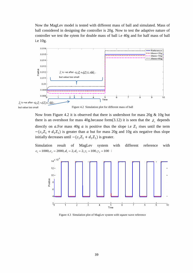
Now the MagLev model is tested with different mass of ball and simulated. Mass of

ball considered in designing the controller is 20g. Now to test the adaptive nature of

controller we test the sytem for double mass of ball i.e 40g and for half mass of ball

i.e 10g.

Figure 4.2 Simulation plot for different mass of ball

Now from Figure 4.2 it is observed that there is undershoot for mass 20g & 10g but

there is an overshoot for mass 40g.because form(3.12) it is seen that the 1Z depends

directly on .For mass 40g is positive thus the slope i.e rises until the term

is greater than but for mass 20g and 10g is negative thus slope

initially decreases until is greater.

Simulation result of MagLev system with different reference with

1 2 1 2 1 21000, 2000, 2, 2, 100, 100c c d d :

Figure 4.3 Simulation plot of MagLev system with sqaure wave reference

is –ve after ,

but value too small

is +ve after ,

but value too small

40

Figure 4.4 Simulation plot of MagLev system with Sine wave reference

However control signal values comes out to be very high in this controller as shown

in Figure 4.5 for step reference. During the time of parameter estimating and state

estimating the control values comes out to be very high.

Figure 4.5 Control signal values for step reference.

4.3 SIMULATION OF NESIC BACKSTEPPING CONTROLLER ON MAGLEV

SYSTEM

The Figure 4.6 shows tracking performance of MagLev system for different 1 2 and c c

values. It is observed that with increase of 1 2 and c c values the tracking error reduces.

However it is found that with increase of 1 2 and c c values the control signal values

also increases. Thus a tradeoff is taken between tracking error and control signal

values. Here 1 2 and c c values are set much less than previous controller method. The

control values also come out to be very less as seen in Figure 4.7.

41

Figure 4.6 Simulation plot for step reference with different 1 2&c c values

It is observed that there is an undershoot initially which is reasoned out as the time

taken by filter parameter „ ‟ to be same with auxiliary control „ ‟ .

Figure 4.7 Plot of error between auxiliary control and stabilizing function

Now simulation is done for different reference inputs.

Figure 4.8 Simulation result for square wave reference

42

Figure 4.9 Simulation result for Sine wave as reference

4.4 SIMULATION OF MAGLEV SYSTEM WITH 2DOF PID

CONTROLLER

The 1P gain of forward loop PI controller is set so as to achieve fast response. Thus for

different values of 1P the Maglev model with 2DOF PID is run.

Figure 4.10 Simulation results of MagLev model with different value of 1P

It is seen from Figure 4.10 that there is an initial overshoot which can be reasoned out

as sensor offset.

With increase of 1P value in positive direction the overshoot increases and with

increase in negative direction the overshoot decreases but it is seen there is an

undershoot as for large negative value of1P .

43

Thus 1P value is set as -1

Tracking for different reference signal is shown in figure

Figure 4.11 Simulation result of MagLev system with square wave reference

Figure 4.12 Simulation result of MagLev system with Sine wave reference

4.5 COMPARISION OF THREE CONTROLLERS

It is observed from Figure 4.13 that all three controllers have very good tracking

performance. However settling time of 2DOF PID is more than other. There is an

initial overshoot for 2DOF PID and undershoot for backstepping on Euler

approximate model.

44

Figure 4.13 Plot of all controller for square wave reference

Figure 4.13 Plot of all controller for sine wave reference

The desirable control output from controller is from -5V to +5V. However the control

output from backstepping controller is in range of 200 and during parameter tuning

the controller output comes in range of 2000. However backstepping based on Euler

approximate model it is observed that the controller output comes in range of 0.5. For

2DOF PID also it is observed that the controller output comes in range of 1.

45

Figure 4.15 Plot of all controller control values

Table 4.5.1 Comparison of all controller performance

CONTROLLER SETTLING TIME

(Seconds)

TRACKING ERROR

(millimeter)

CONTROLLER OUTPUT

Adaptive backstepping 0.2 0.1 2000

Nesic backstepping 0.3 0.1 .5

2DOF PID 1 0.1 1

4.6 EXPERIMENTAL RESULT OF 2DOF CONTROLLER

Figure 4.16 Experimental setup

Control algorithm implementation

Analogue control interface

Magnetic Levitation system Levitated ball by controller

46

4.6.1: 2DOF PID with P1 values:

2DOF PID is tested with different forward path proportional control values. It is

observed that for P1 values greater than -1 in negative value the undershoot is not

being able to control as a result the levitated ball falls down. Similarly for P1 value

higher than 1 , the overshoot is not able to being contained and is attracted to magnet.

The Figure 4.17 shows for different P1 values the MagLev setup response for square

wave reference. It is observed that for P1 =-1 best result is achieved.

Figure 4.17 2DOF PID with different P1 values 0,-1,1

4.6.2: Comparison of 2DOF PID with 1DOF PID in experimental

setup

Now a 2DOF PID is compared with 1DOF PID where it is observed that for 2DOF

apart from the initial overshoot there is no overshoot. However for 1DOF PID it is

observed that the overshoots are present. With overshoot the system robustness is also

decreased. Thus 1DOF is more venerable to instability than 2DOF PID in case of

disturbance. A comparison 1DOF PID is done with 2DOF PID is shown in Figure

4.18.

Figure 4.18 Comparison of 2DOF PID and 1DOF PID

With different P1 values speed of response changes

Shows 1DOF PID has high overshoot and

2DOF PID has very less overshoot. The P1

value is taken as -1 and rest all values are

same for both

47

Table 4.6.1 Comparison of experimental results of 2DOF PID and 1DOF PID.

CONTROLLER RISE TIME

(Seconds)

SETTLING TIME

(Seconds)

TRACKING

ERROR

(millimeter)

OVERSHOOT

(millimeter)

2DOF PID 1 1.5 0 0.5

1DOF PID 0.4 1.5 0 1.3

4.7 SUMMARY OF CHAPTER

In this chapter simulation results of all three controllers are presented. Experimental

validation of 2DOF PID controller is done and a comparison with 1DOF PID is done.

A detail analysis of performance of all controllers has been done in chapter.

48

CHAPTER 5

CONCLUSION AND SUGGETION OF

FUTURE WORK

CONCLUSION

SUGGESTION OF FUTURE WORK

49

5.1 CONCLUSION

In this thesis a detailed modeling and controller design for MagLev system was

carried out. Validation of controller was done in simulation and experiment.

Firstly adaptive backstepping controller was designed. The only output of MagLev

system is position of levitated body. Since all sates are not available in output a state

estimator was designed. However for backstepping strict output feedback form is

required. Kreisselmeier filter was implemented to estimate the immeasurable state.

Kreisselmeier filter also preserves the strict feedback form. The filter was able to

estimate the state in 0.5 seconds. The simulation result shows excellent tracking

performance of the proposed controller. The error in tracking comes out to be less

than 0.1milimeter.

It was observed that adaptive backstepping controller has control output more than

that of our required control signal i.e +5V and -5V, thus a modification was made to

backstepping controller. Backstepping on Euler approximate model shows excellent

tracking with control value less than 1V. The error value here comes out be 0.5

millimeter. However it was observed that the controller could not be applied to real

time experiment as the real time implementation can be only carried by running the

Simulink on “fixed time” solver type with constrain on sampling time as 0.001sec.

The proposed controller runs finely with variable time

For real time experiment implementation 2DOF PID controller was proposed. The

controller was tested on magnetic levitation setup. The experimental result shows

excellent tracking with tracking error of 0.5 millimeter. The controller was also tested

with small external disturbance to the levitated ball.

5.2 FUTURE WORK

.

The magnetic levitation hardware which is provided can be interfaced with computer

with Simulink model. The Simulink model has to be run with „fixed time type solver‟.

At present the backstepping based on Euler approximate model is running finely in

„variable time type solver‟ but in „fixed time type solver‟ the controller is not being

able to track the reference. The controller is only being able to show proper tracking

with sampling time of 0.00001 seconds. The problem might be due the estimator

which is designed according to continuous time system and the taking Euler

approximate of the estimator model. The estimator approximation is not taken into

account in designing the controller.The possible solution can be designing the

controller which takes the estimator Euler approximation into account or by designing

a new estimator which preserves strict feedback form of backstepping.

50

References

[1] Earnshaw, Samuel (1842). "On the Nature of the Molecular Forces which Regulate the

Constitution of the Luminiferous Ether". Trans. Camb. Phil. Soc. 7: 97–112.

[2] Evershed, S., “A frictionless motor meter.” J. Instn elect. Engrs 1900, 29,pp. 743-796.

[3] Faus, H. T, “Magnetic suspension.” U.S. Pat. no. 2315408, 1943 GE (U.S.A.).

[4] Ferranti, S. Z. “Magnetic suspension for electricity meter spindles.” Br. Pat. no. 590292,

1947.

[5] Arkadiev, V. “Hovering of a magnet over a superconductor.” Fiz. Zh. 1945 9,pp 148.

[6] Arkadiev, V. “A floating magnet.” Nature, Lond. 1947 160 (4062),pp 330.

[7] Kemper, H. “Overhead suspension railway with wheel-less vehicles employing magnetic

suspension from iron rails.” 1937 German Pat. nos. 643316, 64402,.

[8] Kemper, H. “Suspension by electromagnetic forces.” Elektrotech. Z., 1938, 59,pp. 391-

395.

[9] Holmes, F. T. “Axial magnetic suspension.” Rev. scient. Instrum. 1937, 8, pp 444-447.

[10] Beams, J. W. “High rotation speeds.” J. appl. Phys. 1973, 8, pp 795-806

[11] Simon, I. “Forces acting on superconductors in magnetic fields.” J. appl. Phys., 1953,

24,pp 19-24.

[12] Culver et. al. “Application of superconductivity to inertial navigation.” Raud Corp, Santa

Monica”, U.S.A, 1957, Rep. no. R363.

[13] Davis, L. C. “Drag force on a magnet moving near a thin conductor”. J appl. Phys. 1972

43, 4256-4257.

[14] Powell, J. R. The magnetic road; a new form of transport. In ASME, Railroad

Conference, Papker 63-RR4. 1963

[15] Powell, J. R. & Danby, G. R. “High speed transport by magnetically suspended trains.

ASME”, Publ no. 66WA/RR5, 1966.

51

[16] Yaghoubi Hamid, “Practical Application of Magnetic Levitation Technology” Final

report Iran Maglev Technology (IMT), sep 2012

[17] Thornton D. Richard, “Efficient and Affordable Maglev opportunities in the United

States” IEEE, 2009 Vol.97

[18] Huang Chao-Hing et al “Adaptive nonlinear control of repulsive MAGLEV suspension

systems”,IEEE conference , 1999 pp 1734-1739.

[19] Yang Zi Jiang et al “Adaptive robust nonlinear control of magnetic levitation

system”,Automatica , 2001,pp 1125-1131.

[20] Lepetic et al., "Predictive control based on fuzzy model: a case study," Fuzzy Systems,

2001. The 10th IEEE International Conference on , vol.2, no., pp.868,871 vol.3, 2-5 Dec.

2001.

[21] Jalili Kharaajoo Mahadi, “Sliding mode control of voltage controlled magnetic levitation

systems” IEEE Conference pp 83-86, 2003

[22] Fallaha Charles et al, “Real time implementation of a sliding mode regulator for current

controlled magnetic levitation system”, 2005

[23] Cho Dan, “Sliding mode and classical control magnetic levitation system”, IEEE

Control Magazine, 1993

[24] Yang Jun et al “Robust control of nonlinear MAGLEV suspension system with

mismatch uncertainties via DOBC approach ”,ISA Trans pp 389-396, 2001

[25] Ghosh et al “Design and implementation of a 2-DOF PID compensation for magnetic

levitation system”,ISA Trans pp 1216-1222, 2014

[26] Kirtley Jr J.L, “Introduction to Power System” Class note chapter 8 “ElectroMagnetic

Forces and Loss Mechanisms”

[27] Feedback Instrument Magnetic Levitation manual

[28] Krstic M.et al “Nonlinear and adaptive control design” (Wiley, New York, 1995)

[29] Yang Z.J: “Adaptive robust output-feedback control of a magnetic levitation system by

K-filter approach”, IEEE. Trans. Ind. Electron, 2008, 55, (1), pp. 390–399

52

[30] Yang Z.J. et al. “A novel robust nonlinear motion controller with disturbance observer”,

IEEE Trans. Control Syst. Technol., 2008, 16, (1), pp. 137–147

[31] Yang Z J et al, “Robust non-linear output-feedback control of a magnetic levitation

system by K- Filter approach” ,IET Control Theory and Applications,2008.0253,pp

852-864

[32] Mishra Anand Ku et al, “Modeling and Simulation of Levitating Ball by Electromagnet

using Bond Graph”, iNaCoMM , 2013,pp 42-48

[33] D.Nesic and A.R.Teel, “Backstepping on the Euler approximate model for stabilization

of sampled –data nonlinear systems.” IEEE Conference, 2001, pp1737-1742

[34] Beltran-Carbajal F.et al, “Output feedback control of a mechanical system using

magnetic levitation”,ISA Trans,2015

[35] Herbert, et al, “Electromechanical Dynamics Part II”, Masachusetts Institute of

Technology: MIT Open Course,3 Vol

[36] <http://maglevtrainenglishpac.weebly.com/differeneces-between-eds-and-ems.html>

,Acessed online 27/5/2015

[37] <http://www.e-driveonline.com/main/wp-content/uploads/2012/05/a1-300x180.gif>

,Acessed online 27/5/2015

[38] <https://mix.msfc.nasa.gov/IMAGES/HIGH/9906088.jpg> ,Acessed online 27/5/2015

[39] <http://www.foxnews.com/tech/2014/05/14/navy-to-test-electromagnetic-catapult-on-

carrier/> ,Acessed online 27/5/2015

[40] <http://www.robotliving.com/robot-news/magnetic-levitating-microbots/> ,Acessed

online 27/5/2015

[41] Jayawant.B, “Review Lecture.Electromagnetic Suspension and Levitation Techniques”,

Proceeding of the Royal Society of London.series”, Mathematical and Physical Science,

Vol.416, pp 245-320, 1988

[42] Khamesee, M.B et al. "Design and control of a microrobotic system using magnetic

levitation," Mechatronics, IEEE/ASME Transactions on , vol.7, no.1, pp.1,14, Mar 2002