
Control Theory: History, Mathematical Achievements and - BCAM
62
Bol. Soc. Esp. Mat. Apl. n o 0 (0000), 1–62 Control Theory: History, Mathematical Achievements and Perspectives * E. Fern ´ andez-Cara 1 and E. Zuazua 2 1 Departamento de Ecuaciones Diferenciales y An´alisis Num´ erico, Universidad de Sevilla 2 Departamento de Matem´aticas, Universidad Aut´onoma de Madrid [email protected], [email protected] Abstract These notes are devoted to present some of the mathematical milestones of Control Theory. To do that, we first overview its origins and some of the main mathematical achievements. Then, we discuss the main domains of Sciences and Technologies where Control Theory arises and applies. This forces us to address modelling issues and to distinguish between the two main control theoretical approaches, controllability and optimal control, discussing the advantages and drawbacks of each of them. In order to give adequate formulations of the main questions, we have introduced some of the most elementary mathematical material, avoiding unnecessary technical difficulties and trying to make the paper accessible to a large class of readers. The subjects we address range from the basic concepts related to the dynamical systems approach to (linear and nonlinear) Mathematical Programming and Calculus of Variations. We also present a simplified version of the outstanding results by Kalman on the controllability of linear finite dimensional dynamical systems, Pontryaguin’s maximum principle and the principle of dynamical programming. Some aspects related to the complexity of modern control systems, the discrete versus continuous modelling, the numerical approximation of control problems and its control theoretical consequences are also discussed. Finally, we describe some of the major challenging applications in Control Theory for the XXI Century. They will probably influence strongly the development of this discipline in the near future. * The authors have been partially financed by D.G.E.S.-Espa˜ na, respectively Grants BFM2000-1317 and BFM2002-03345. 1
Transcript of Control Theory: History, Mathematical Achievements and - BCAM
Bol. Soc. Esp. Mat. Apl. no0 (0000), 1–62
Control Theory: History, Mathematical Achievements andPerspectives *
E. Fernandez-Cara1 and E. Zuazua2
1 Departamento de Ecuaciones Diferenciales y Analisis Numerico,Universidad de Sevilla
2 Departamento de Matematicas,Universidad Autonoma de Madrid
[email protected], [email protected]
Abstract
These notes are devoted to present some of the mathematicalmilestones of Control Theory. To do that, we first overview its originsand some of the main mathematical achievements. Then, we discuss themain domains of Sciences and Technologies where Control Theory arisesand applies. This forces us to address modelling issues and to distinguishbetween the two main control theoretical approaches, controllability andoptimal control, discussing the advantages and drawbacks of each of them.
In order to give adequate formulations of the main questions, we haveintroduced some of the most elementary mathematical material, avoidingunnecessary technical difficulties and trying to make the paper accessibleto a large class of readers.
The subjects we address range from the basic concepts related tothe dynamical systems approach to (linear and nonlinear) MathematicalProgramming and Calculus of Variations. We also present a simplifiedversion of the outstanding results by Kalman on the controllability oflinear finite dimensional dynamical systems, Pontryaguin’s maximumprinciple and the principle of dynamical programming.
Some aspects related to the complexity of modern control systems,the discrete versus continuous modelling, the numerical approximationof control problems and its control theoretical consequences are alsodiscussed.
Finally, we describe some of the major challenging applications inControl Theory for the XXI Century. They will probably influencestrongly the development of this discipline in the near future.
*The authors have been partially financed by D.G.E.S.-Espana, respectivelyGrants BFM2000-1317 and BFM2002-03345.
1
2 E. Fernandez-Cara and E. Zuazua
Key words : Control Theory, optimal control, controllability, differentialequations, feedback, Optimization, Calculus of Variations.
AMS subject classifications : 49J15, 49J20, 70Q05, 93B, 93C
1. Introduction
This article is devoted to present some of the mathematical milestones ofControl Theory. We will focus on systems described in terms of ordinarydifferential equations. The control of (deterministic and stochastic) partialdifferential equations remains out of our scope. However, it must be underlinedthat most ideas, methods and results presented here do extend to this moregeneral setting, which leads to very important technical developments.
The underlying idea that motivated this article is that Control Theoryis certainly, at present, one of the most interdisciplinary areas of research.Control Theory arises in most modern applications. The same could besaid about the very first technological discoveries of the industrial revolution.On the other hand, Control Theory has been a discipline where manymathematical ideas and methods have melt to produce a new body of importantMathematics. Accordingly, it is nowadays a rich crossing point of Engineeringand Mathematics.
Along this paper, we have tried to avoid unnecessary technical difficulties,to make the text accessible to a large class of readers. However, in order tointroduce some of the main achievements in Control Theory, a minimal bodyof basic mathematical concepts and results is needed. We develop this materialto make the text self-contained.
These notes contain information not only on the main mathematical resultsin Control Theory, but also about its origins, history and the way applicationsand interactions of Control Theory with other Sciences and Technologies haveconducted the development of the discipline.
The plan of the paper is the following. Section 2 is concerned with theorigins and most basic concepts. In Section 3 we study a simple but veryinteresting example: the pendulum. As we shall see, an elementary analysis ofthis simple but important mechanical system indicates that the fundamentalideas of Control Theory are extremely meaningful from a physical viewpoint.
In Section 4 we describe some relevant historical facts and also someimportant contemporary applications. There, it will be shown that ControlTheory is in fact an interdisciplinary subject that has been strongly involved inthe development of the contemporary society.
In Section 5 we describe the two main approaches that allow to give rigorousformulations of control problems: controllability and optimal control. We alsodiscuss their mutual relations, advantages and drawbacks.
In Sections 6 and 7 we present some basic results on the controllability oflinear and nonlinear finite dimensional systems. In particular, we revisit theKalman approach to the controllability of linear systems, and we recall the useof Lie brackets in the control of nonlinear systems, discussing a simple example
An Overview of Control Theory 3
of a planar moving square car.In Section 8 we discuss how the complexity of the systems arising in modern
technologies affects Control Theory and the impact of numerical approximationsand discrete modelling, when compared to the classical modelling in the contextof Continuum Mechanics.
In Section 9 we describe briefly two beautiful and extremely importantchallenging applications for Control Theory in which, from a mathematicalviewpoint, almost all remains to be done: laser molecular control and the controlof floods.
In Section 10 we present a list of possible future applications and lines ofdevelopment of Control Theory: large space structures, Robotics, biomedicalresearch, etc.
Finally, we have included two Appendices, where we recall briefly two ofthe main principles of modern Control Theory, namely Pontryagin’s maximumprinciple and Bellman’s dynamical programming principle.
2. Origins and basic ideas, concepts and ingredients
The word control has a double meaning. First, controlling a system can beunderstood simply as testing or checking that its behavior is satisfactory. In adeeper sense, to control is also to act, to put things in order to guarantee thatthe system behaves as desired.
S. Bennet starts the first volume of his book [2] on the history of ControlEngineering quoting the following sentence of Chapter 3, Book 1, of themonograph “Politics” by Aristotle:
“. . . if every instrument could accomplish its own work, obeying oranticipating the will of others . . . if the shuttle weaved and the picktouched the lyre without a hand to guide them, chief workmen wouldnot need servants, nor masters slaves.”
Figure 1: Aristotle(384–322 B.C.).
This sentence by Aristotle describes in a rathertransparent way the guiding goal of Control Theory:the need of automatizing processes to let the humanbeing gain in liberty, freedom, and quality of life.
Let us indicate briefly how control problems arestated nowadays in mathematical terms. To fix ideas,assume we want to get a good behavior of a physicalsystem governed by the state equation
A(y) = f(v). (1)
Here, y is the state, the unknown of the systemthat we are willing to control. It belongs to a vectorspace Y . On the other hand, v is the control. It
4 E. Fernandez-Cara and E. Zuazua
belongs to the set of admissible controls Uad . This is the variable that we canchoose freely in Uad to act on the system.
Let us assume that A : D(A) ⊂ Y 7→ Y and f : Uad 7→ Y are two given(linear or nonlinear) mappings. The operator A determines the equation thatmust be satisfied by the state variable y, according to the laws of Physics. Thefunction f indicates the way the control v acts on the system governing thestate. For simplicity, let us assume that, for each v ∈ Uad , the state equation(1) possesses exactly one solution y = y(v) in Y . Then, roughly speaking, tocontrol (1) is to find v ∈ Uad such that the solution to (1) gets close to thedesired prescribed state. The “best” among all the existing controls achievingthe desired goal is frequently referred to as the optimal control.
This mathematical formulation might seem sophisticated or even obscurefor readers not familiar with this topic. However, it is by now standard and ithas been originated naturally along the history of this rich discipline. One ofthe main advantages of such a general setting is that many problems of verydifferent nature may fit in it, as we shall see along this work.
As many other fields of human activities, the discipline of Control existedmuch earlier than it was given that name. Indeed, in the world of living species,organisms are endowed with sophisticated mechanisms that regulate the varioustasks they develop. This is done to guarantee that the essential variables arekept in optimal regimes to keep the species alive allowing them to grow, developand reproduce.
Thus, although the mathematical formulation of control problems isintrinsically complex, the key ideas in Control Theory can be found in Nature,in the evolution and behavior of living beings.
The first key idea is the feedback concept. This term was incorporated toControl Engineering in the twenties by the engineers of the “Bell TelephoneLaboratory” but, at that time, it was already recognized and consolidated inother areas, such as Political Economics.
Essentially, a feedback process is the one in which the state of the systemdetermines the way the control has to be exerted at any time. This is relatedto the notion of real time control, very important for applications. In theframework of (1), we say that the control u is given by a feedback law if weare able to provide a mapping G : Y 7→ Uad such that
u = G(y), where y = y(u), (2)
i.e. y solves (1) with v replaced by u.Nowadays, feedback processes are ubiquitous not only in Economics, but
also in Biology, Psychology, etc. Accordingly, in many different related areas,the cause-effect principle is not understood as a static phenomenon any more,but it is rather being viewed from a dynamical perspective. Thus, we can speakof the cause-effect-cause principle. See [33] for a discussion on this and otherrelated aspects.
The second key idea is clearly illustrated by the following sentence byH.R. Hall in [17] in 1907 and that we have taken from [2]:
An Overview of Control Theory 5
“It is a curious fact that, while political economists recognize thatfor the proper action of the law of supply and demand there must befluctuations, it has not generally been recognized by mechanicians inthis matter of the steam engine governor. The aim of the mechanicaleconomist, as is that of the political economist, should be not to doaway with these fluctuations all together (for then he does away withthe principles of self-regulation), but to diminish them as much aspossible, still leaving them large enough to have sufficient regulatingpower.”
The need of having room for fluctuations that this paragraph evokes isrelated to a basic principle that we apply many times in our daily life. Forinstance, when driving a car at a high speed and needing to brake, we usuallytry to make it intermittently, in order to keep the vehicle under control at anymoment. In the context of human relationships, it is also clear that insistingpermanently in the same idea might not be precisely the most convincingstrategy.
The same rule applies for the control of a system. Thus, to control a systemarising in Nature or Technology, we do not have necessarily to stress the systemand drive it to the desired state immediately and directly. Very often, it is muchmore efficient to control the system letting it fluctuate, trying to find a harmonicdynamics that will drive the system to the desired state without forcing it toomuch. An excess of control may indeed produce not only an inadmissible costbut also irreversible damages in the system under consideration.
Another important underlying notion in Control Theory is Optimization.This can be regarded as a branch of Mathematics whose goal is to improvea variable in order to maximize a benefit (or minimize a cost). This isapplicable to a lot of practical situations (the variable can be a temperature,a velocity field, a measure of information, etc.). Optimization Theory andits related techniques are such a broad subject that it would be impossibleto make a unified presentation. Furthermore, a lot of recent developments inInformatics and Computer Science have played a crucial role in Optimization.Indeed, the complexity of the systems we consider interesting nowadays makesit impossible to implement efficient control strategies without using appropriate(and sophisticated) software.
In order to understand why Optimization techniques and Control Theoryare closely related, let us come back to (1). Assume that the set of admissiblecontrols Uad is a subset of the Banach space U (with norm ‖ · ‖U ) and the statespace Y is another Banach space (with norm ‖ · ‖Y ). Also, assume that thestate yd ∈ Y is the preferred state and is chosen as a target for the state of thesystem. Then, the control problem consists in finding controls v in Uad suchthat the associated solution coincides or gets close to yd.
It is then reasonable to think that a fruitful way to choose a good control vis by minimizing a cost function of the form
J(v) =12‖y(v)− yd‖2Y ∀v ∈ Uad (3)
6 E. Fernandez-Cara and E. Zuazua
or, more generally,
J(v) =12‖y(v)− yd‖2Y +
µ
2‖v‖2U ∀v ∈ Uad , (4)
where µ ≥ 0.These are (constrained) extremal problems whose analysis corresponds to
Optimization Theory.It is interesting to analyze the two terms arising in the functional J in (4)
when µ > 0 separately, since they play complementary roles. When minimizingthe functional in (4), we are minimizing the balance between these two terms.The first one requires to get close to the target yd while the second one penalizesusing too much costly control. Thus, roughly speaking, when minimizing J weare trying to drive the system to a state close to the target yd without too mucheffort.
We will give below more details of the connection of Control Theory andOptimization below.
So far, we have mentioned three main ingredients arising in Control Theory:the notion of feedback, the need of fluctuations and Optimization. But ofcourse in the development of Control Theory many other concepts have beenimportant.
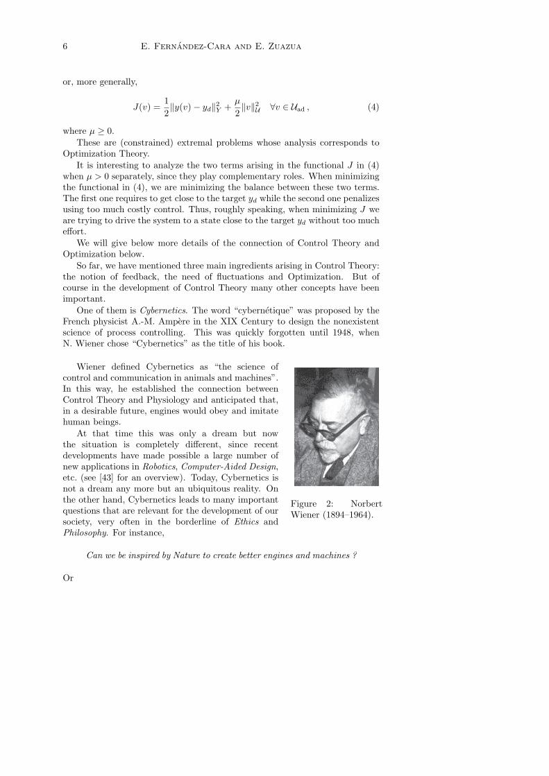
One of them is Cybernetics. The word “cybernetique” was proposed by theFrench physicist A.-M. Ampere in the XIX Century to design the nonexistentscience of process controlling. This was quickly forgotten until 1948, whenN. Wiener chose “Cybernetics” as the title of his book.
Figure 2: NorbertWiener (1894–1964).
Wiener defined Cybernetics as “the science ofcontrol and communication in animals and machines”.In this way, he established the connection betweenControl Theory and Physiology and anticipated that,in a desirable future, engines would obey and imitatehuman beings.
At that time this was only a dream but nowthe situation is completely different, since recentdevelopments have made possible a large number ofnew applications in Robotics, Computer-Aided Design,etc. (see [43] for an overview). Today, Cybernetics isnot a dream any more but an ubiquitous reality. Onthe other hand, Cybernetics leads to many importantquestions that are relevant for the development of oursociety, very often in the borderline of Ethics andPhilosophy. For instance,
Can we be inspired by Nature to create better engines and machines ?
Or
An Overview of Control Theory 7
Is the animal behavior an acceptable criterium to judge theperformance of an engine ?
Many movies of science fiction describe a world in which machines donot obey any more to humans and humans become their slaves. This is theopposite situation to the one Control Theory has been and is looking for. Thedevelopment of Science and Technology is obeying very closely to the predictionsmade fifty years ago. Therefore, it seems desirable to deeply consider and reviseour position towards Cybernetics from now on, many years ahead, as we dopermanently in what concerns, for instance, Genetics and the possibilities itprovides to intervene in human reproduction.
3. The pendulum
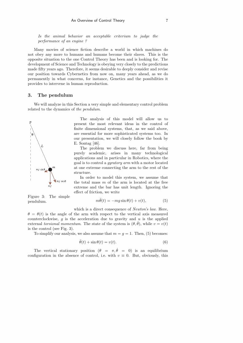
We will analyze in this Section a very simple and elementary control problemrelated to the dynamics of the pendulum.
Figure 3: The simplependulum.
The analysis of this model will allow us topresent the most relevant ideas in the control offinite dimensional systems, that, as we said above,are essential for more sophisticated systems too. Inour presentation, we will closely follow the book byE. Sontag [46].
The problem we discuss here, far from beingpurely academic, arises in many technologicalapplications and in particular in Robotics, where thegoal is to control a gyratory arm with a motor locatedat one extreme connecting the arm to the rest of thestructure.
In order to model this system, we assume thatthe total mass m of the arm is located at the freeextreme and the bar has unit length. Ignoring theeffect of friction, we write
mθ(t) = −mg sin θ(t) + v(t), (5)
which is a direct consequence of Newton’s law. Here,θ = θ(t) is the angle of the arm with respect to the vertical axis measuredcounterclockwise, g is the acceleration due to gravity and u is the appliedexternal torsional momentum. The state of the system is (θ, θ), while v = v(t)is the control (see Fig. 3).
To simplify our analysis, we also assume that m = g = 1. Then, (5) becomes:
θ(t) + sin θ(t) = v(t). (6)
The vertical stationary position (θ = π, θ = 0) is an equilibriumconfiguration in the absence of control, i.e. with v ≡ 0. But, obviously, this
8 E. Fernandez-Cara and E. Zuazua
is an unstable equilibrium. Let us analyze the system around this configuration,to understand how this instability can be compensated by means of the appliedcontrol force v.
Taking into account that sin θ ∼ π − θ near θ = π, at first approximation,the linearized system with respect to the variable ϕ = θ − π can be written inthe form
ϕ− ϕ = v(t). (7)
The goal is then to drive (ϕ, ϕ) to the desired state (0, 0) for all small initialdata, without making the angle and the velocity too large along the controlledtrajectory.
The following control strategy is in agreement with common sense: whenthe system is to the left of the vertical line, i.e. when ϕ = θ − π > 0, we pushthe system towards the right side, i.e. we apply a force v with negative sign; onthe other hand, when ϕ < 0, it seems natural to choose v > 0.
This suggests the following feedback law, in which the control is proportionalto the state:
v = −αϕ, with α > 0. (8)
In this way, we get the closed loop system
ϕ + (α− 1)ϕ = 0. (9)
It is important to understand that, solving (9), we simultaneously obtainthe state (ϕ, ϕ) and the control v = −αϕ. This justifies, at least in this case,the relevance of a feedback law like (8).
The roots of the characteristic polynomial of the linear equation (9) arez = ±√1− α. Hence, when α > 1, the nontrivial solutions of this differentialequation are oscillatory. When α < 1, all solutions diverge to ±∞ as t → ±∞,except those satisfying
ϕ(0) = −√1− α ϕ(0).
Finally, when α = 1, all nontrivial solutions satisfying ϕ(0) = 0 are constant.Thus, the solutions to the linearized system (9) do not reach the desired
configuration (0, 0) in general, independently of the constant α we put in (8).This can be explained as follows. Let us first assume that α < 1. When
ϕ(0) is positive and small and ϕ(0) = 0, from equation (9) we deduce thatϕ(0) > 0. Thus, ϕ and ϕ grow and, consequently, the pendulum goes awayfrom the vertical line. When α > 1, the control acts on the correct directionbut with too much inertia.
The same happens to be true for the nonlinear system (6).The most natural solution is then to keep α > 1, but introducing an
additional term to diminish the oscillations and penalize the velocity. In thisway, a new feedback law can be proposed in which the control is given as alinear combination of ϕ and ϕ:
v = −αϕ− βϕ, with α > 1 and β > 0. (10)
An Overview of Control Theory 9
The new closed loop system is
ϕ + βϕ + (α− 1)ϕ = 0, (11)
whose characteristic polynomial has the following roots
−β ±√
β2 − 4(α− 1)2
. (12)
Now, the real part of the roots is negative and therefore, all solutionsconverge to zero as t → +∞. Moreover, if we impose the condition
β2 > 4(α− 1), (13)
we see that solutions tend to zero monotonically, without oscillations.This simple model is rich enough to illustrate some systematic properties of
control systems:
• Linearizing the system is an useful tool to address its control, althoughthe results that can be obtained this way are only of local nature.
• One can obtain feedback controls, but their effects on the system arenot necessarily in agreement with the very first intuition. Certainly, the(asymptotic) stability properties of the system must be taken into account.
• Increasing dissipation one can eliminate the oscillations, as we haveindicated in (13).
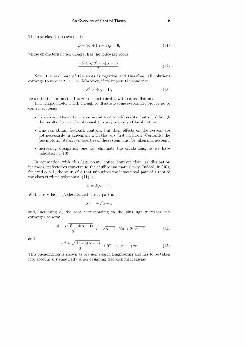
In connection with this last point, notice however that, as dissipationincreases, trajectories converge to the equilibrium more slowly. Indeed, in (10),for fixed α > 1, the value of β that minimizes the largest real part of a root ofthe characteristic polynomial (11) is
β = 2√
α− 1.
With this value of β, the associated real part is
σ∗ = −√α− 1
and, increasing β, the root corresponding to the plus sign increases andconverges to zero:
−β +√
β2 − 4(α− 1)2
> −√α− 1 ∀β > 2√
α− 1 (14)
and−β +
√β2 − 4(α− 1)
2→ 0− as β → +∞. (15)
This phenomenon is known as overdamping in Engineering and has to be takeninto account systematically when designing feedback mechanisms.
10 E. Fernandez-Cara and E. Zuazua
At the practical level, implementing the control (10) is not so simple, sincethe computation of v requires knowing the position ϕ and the velocity ϕ atevery time.
Let us now describe an interesting alternative. The key idea is to evaluateϕ and ϕ only on a discrete set of times
0, δ, 2δ, . . . , kδ, . . .
and modify the control at each of these values of t. The control we get this wayis kept constant along each interval [kδ, (k + 1)δ].
Computing the solution to system (7), we see that the result of applying theconstant control vk in the time interval [kδ, (k + 1)δ] is as follows:
(ϕ(kδ + δ)ϕ(kδ + δ)
)= A
(ϕ(kδ)ϕ(kδ)
)+ vk b,
where
A =(
coshδ sinhδsin hδ coshδ
), b =
(coshδ − 1
sinhδ
).
Thus, we obtain a discrete system of the form
xk+1 = (A + bf t)xk ,
where f is the vector such that
vk = f txk .
Observe that, if f is such that the matrix A + bf t is nilpotent, i.e.
[A + bf t]2 = 0,
then we reach the equilibrium in two steps. A simple computation shows thatthis property holds if f t = (f1, f2), with
f1 =1− 2 cos hδ
2(cos hδ − 1), f2 = −1 + 2 cos hδ
2 sin hδ. (16)
The main advantage of using controllers of this form is that we get thestabilization of the trajectories in finite time and not only asymptotically, ast → +∞. The controller we have designed is a digital control and it is extremelyuseful because of its robustness and the ease of its implementation.
The digital controllers we have built are similar and closely related to thebang-bang controls we are going to describe now.
Once α > 1 is fixed, for instance α = 2, we can assume that
v = −2ϕ + w, (17)
so that (7) can be written in the form
ϕ + ϕ = w. (18)
An Overview of Control Theory 11
This is Newton’s law for the vibration of a spring.This time, we look for controls below an admissible cost. For instance, we
impose|w(t)| ≤ 1 ∀t.
The function w = w(t) that, satisfying this constraint, controls the system inminimal time, i.e. the optimal control, is necessarily of the form
w(t) = sgn(p(t)),
where η is a solution ofp + p = 0.
This is a consequence of Pontryagin’s maximum principle (see Appendix 1 formore details).
Therefore, the optimal control takes only the values ±1 and, in practice, itis sufficient to determine the switching times at which the sign of the optimalcontrol changes.
In order to compute the optimal control, let us first compute the solutionscorresponding to the extremal controllers ±1. Using the new variables x1 andx2 with x1 = ϕ and x2 = ϕ, this is equivalent to solve the systems
x1 = x2
x2 = −x1 + 1 (19)
and x1 = x2
x2 = −x1 − 1.(20)
The solutions can be identified to the circumferences in the plane (x1, x2)centered at (1, 0) and (−1, 0), respectively. Consequently, in order to drive(18) to the final state (ϕ, ϕ)(T ) = (0, 0), we must follow these circumferences,starting from the prescribed initial state and switching from one to anotherappropriately.
For instance, assume that we start from the initial state (ϕ, ϕ)(0) = (ϕ0, ϕ1),where ϕ0 and ϕ1 are positive and small (see Fig. 4). Then, we first takew(t) = 1 and solve (19) for t ∈ [0, T1], where T1 is such that x2(T1) = 0, i.e. wefollow counterclockwise the arc connecting the points (ϕ0, ϕ1) and (x1(T1), 0)in the (x1, x2) plane. In a second step, we take w(t) = −1 and solve (20)for t ∈ [T1, T2], where T2 is such that (1 − x1(T2))2 + x2(T2)2 = 1. We thusfollow (again counterclockwise) the arc connecting the points (x1(T1), 0) and(x1(T2), x2(T2)). Finally, we take w(t) = 1 and solve (19) for t ∈ [T2, T3], withT3 such that x1(T3 = x2(T3) = 0.
Similar constructions of the control can be done when ϕ0 ≤ 1 or ϕ1 ≤ 0.In this way, we reach the equilibrium (0, 0) in finite time and we obtain a
feedback mechanismϕ + ϕ = F (ϕ, ϕ),
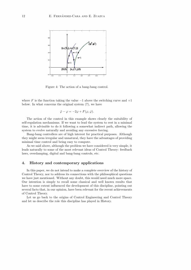
12 E. Fernandez-Cara and E. Zuazua
Figure 4: The action of a bang-bang control.
where F is the function taking the value −1 above the switching curve and +1below. In what concerns the original system (7), we have
ϕ− ϕ = −2ϕ + F (ϕ, ϕ).
The action of the control in this example shows clearly the suitability ofself-regulation mechanisms. If we want to lead the system to rest in a minimaltime, it is advisable to do it following a somewhat indirect path, allowing thesystem to evolve naturally and avoiding any excessive forcing.
Bang-bang controllers are of high interest for practical purposes. Althoughthey might seem irregular and unnatural, they have the advantages of providingminimal time control and being easy to compute.
As we said above, although the problem we have considered is very simple, itleads naturally to some of the most relevant ideas of Control Theory: feedbacklaws, overdamping, digital and bang-bang controls, etc.
4. History and contemporary applications
In this paper, we do not intend to make a complete overview of the history ofControl Theory, nor to address its connections with the philosophical questionswe have just mentioned. Without any doubt, this would need much more space.Our intention is simply to recall some classical and well known results thathave to some extent influenced the development of this discipline, pointing outseveral facts that, in our opinion, have been relevant for the recent achievementsof Control Theory.
Let us go back to the origins of Control Engineering and Control Theoryand let us describe the role this discipline has played in History.
An Overview of Control Theory 13
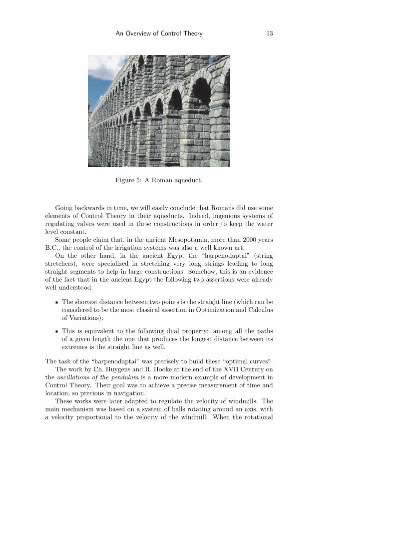
Figure 5: A Roman aqueduct.
Going backwards in time, we will easily conclude that Romans did use someelements of Control Theory in their aqueducts. Indeed, ingenious systems ofregulating valves were used in these constructions in order to keep the waterlevel constant.
Some people claim that, in the ancient Mesopotamia, more than 2000 yearsB.C., the control of the irrigation systems was also a well known art.
On the other hand, in the ancient Egypt the “harpenodaptai” (stringstretchers), were specialized in stretching very long strings leading to longstraight segments to help in large constructions. Somehow, this is an evidenceof the fact that in the ancient Egypt the following two assertions were alreadywell understood:
The shortest distance between two points is the straight line (which can beconsidered to be the most classical assertion in Optimization and Calculusof Variations);
This is equivalent to the following dual property: among all the pathsof a given length the one that produces the longest distance between itsextremes is the straight line as well.
The task of the “harpenodaptai” was precisely to build these “optimal curves”.The work by Ch. Huygens and R. Hooke at the end of the XVII Century on
the oscillations of the pendulum is a more modern example of development inControl Theory. Their goal was to achieve a precise measurement of time andlocation, so precious in navigation.
These works were later adapted to regulate the velocity of windmills. Themain mechanism was based on a system of balls rotating around an axis, witha velocity proportional to the velocity of the windmill. When the rotational
14 E. Fernandez-Cara and E. Zuazua
velocity increased, the balls got farther from the axis, acting on the wings ofthe mill through appropriate mechanisms.
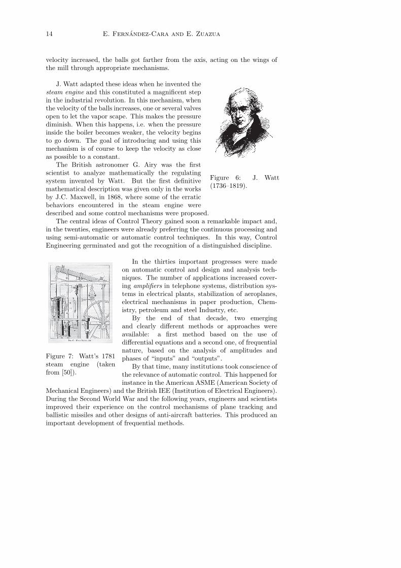
Figure 6: J. Watt(1736–1819).
J. Watt adapted these ideas when he invented thesteam engine and this constituted a magnificent stepin the industrial revolution. In this mechanism, whenthe velocity of the balls increases, one or several valvesopen to let the vapor scape. This makes the pressurediminish. When this happens, i.e. when the pressureinside the boiler becomes weaker, the velocity beginsto go down. The goal of introducing and using thismechanism is of course to keep the velocity as closeas possible to a constant.
The British astronomer G. Airy was the firstscientist to analyze mathematically the regulatingsystem invented by Watt. But the first definitivemathematical description was given only in the worksby J.C. Maxwell, in 1868, where some of the erraticbehaviors encountered in the steam engine weredescribed and some control mechanisms were proposed.
The central ideas of Control Theory gained soon a remarkable impact and,in the twenties, engineers were already preferring the continuous processing andusing semi-automatic or automatic control techniques. In this way, ControlEngineering germinated and got the recognition of a distinguished discipline.
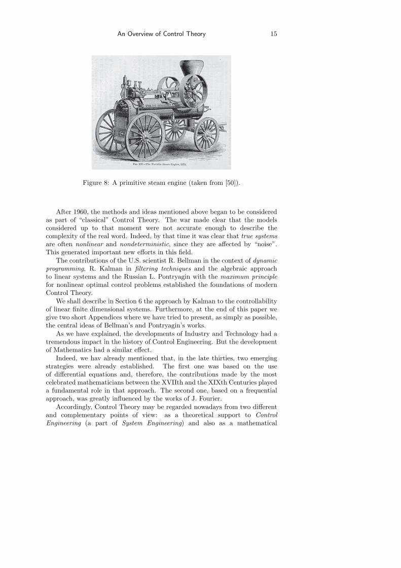
Figure 7: Watt’s 1781steam engine (takenfrom [50]).
In the thirties important progresses were madeon automatic control and design and analysis tech-niques. The number of applications increased cover-ing amplifiers in telephone systems, distribution sys-tems in electrical plants, stabilization of aeroplanes,electrical mechanisms in paper production, Chem-istry, petroleum and steel Industry, etc.
By the end of that decade, two emergingand clearly different methods or approaches wereavailable: a first method based on the use ofdifferential equations and a second one, of frequentialnature, based on the analysis of amplitudes andphases of “inputs” and “outputs”.
By that time, many institutions took conscience ofthe relevance of automatic control. This happened forinstance in the American ASME (American Society of
Mechanical Engineers) and the British IEE (Institution of Electrical Engineers).During the Second World War and the following years, engineers and scientistsimproved their experience on the control mechanisms of plane tracking andballistic missiles and other designs of anti-aircraft batteries. This produced animportant development of frequential methods.
An Overview of Control Theory 15
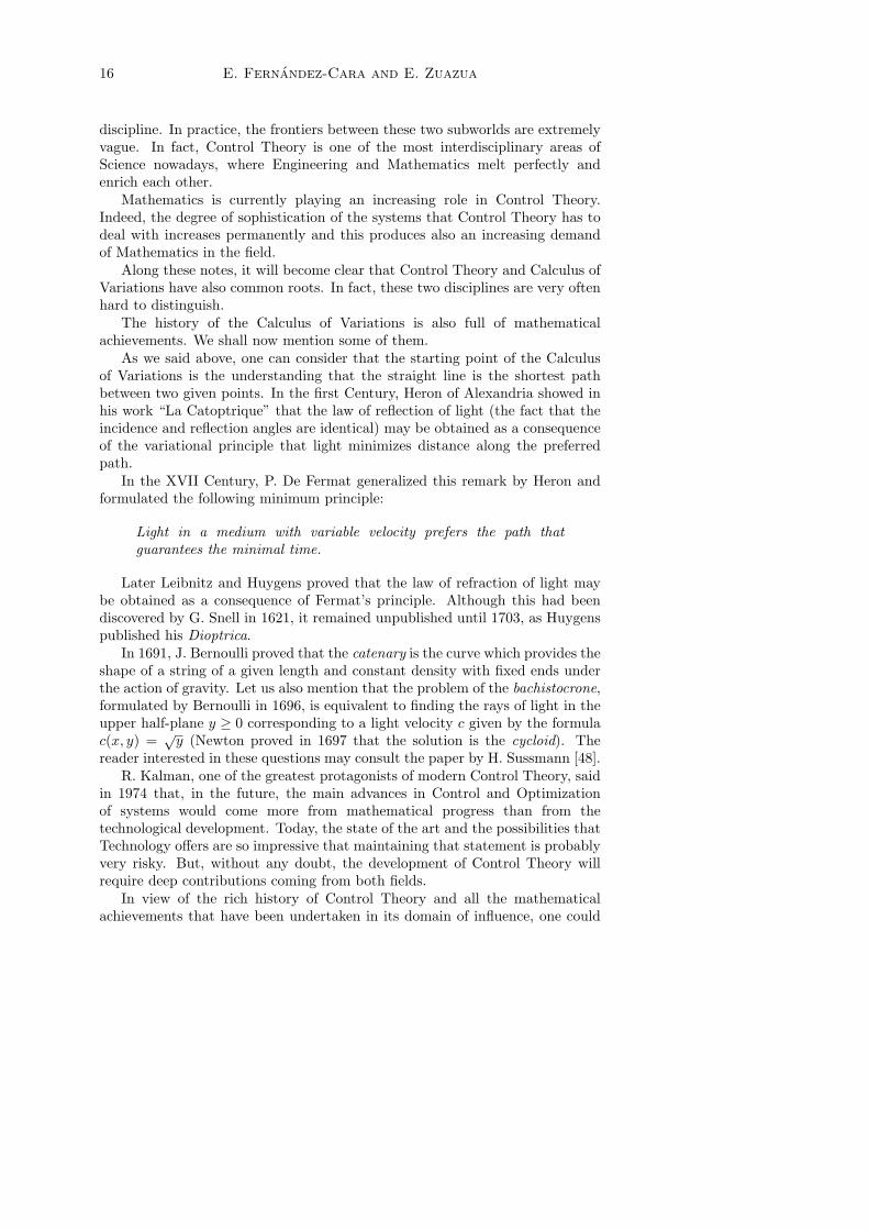
Figure 8: A primitive steam engine (taken from [50]).
After 1960, the methods and ideas mentioned above began to be consideredas part of “classical” Control Theory. The war made clear that the modelsconsidered up to that moment were not accurate enough to describe thecomplexity of the real word. Indeed, by that time it was clear that true systemsare often nonlinear and nondeterministic, since they are affected by “noise”.This generated important new efforts in this field.
The contributions of the U.S. scientist R. Bellman in the context of dynamicprogramming, R. Kalman in filtering techniques and the algebraic approachto linear systems and the Russian L. Pontryagin with the maximum principlefor nonlinear optimal control problems established the foundations of modernControl Theory.
We shall describe in Section 6 the approach by Kalman to the controllabilityof linear finite dimensional systems. Furthermore, at the end of this paper wegive two short Appendices where we have tried to present, as simply as possible,the central ideas of Bellman’s and Pontryagin’s works.
As we have explained, the developments of Industry and Technology had atremendous impact in the history of Control Engineering. But the developmentof Mathematics had a similar effect.
Indeed, we hav already mentioned that, in the late thirties, two emergingstrategies were already established. The first one was based on the useof differential equations and, therefore, the contributions made by the mostcelebrated mathematicians between the XVIIth and the XIXth Centuries playeda fundamental role in that approach. The second one, based on a frequentialapproach, was greatly influenced by the works of J. Fourier.
Accordingly, Control Theory may be regarded nowadays from two differentand complementary points of view: as a theoretical support to ControlEngineering (a part of System Engineering) and also as a mathematical
16 E. Fernandez-Cara and E. Zuazua
discipline. In practice, the frontiers between these two subworlds are extremelyvague. In fact, Control Theory is one of the most interdisciplinary areas ofScience nowadays, where Engineering and Mathematics melt perfectly andenrich each other.
Mathematics is currently playing an increasing role in Control Theory.Indeed, the degree of sophistication of the systems that Control Theory has todeal with increases permanently and this produces also an increasing demandof Mathematics in the field.
Along these notes, it will become clear that Control Theory and Calculus ofVariations have also common roots. In fact, these two disciplines are very oftenhard to distinguish.
The history of the Calculus of Variations is also full of mathematicalachievements. We shall now mention some of them.
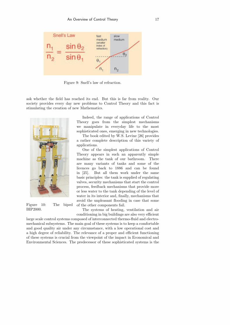
As we said above, one can consider that the starting point of the Calculusof Variations is the understanding that the straight line is the shortest pathbetween two given points. In the first Century, Heron of Alexandria showed inhis work “La Catoptrique” that the law of reflection of light (the fact that theincidence and reflection angles are identical) may be obtained as a consequenceof the variational principle that light minimizes distance along the preferredpath.
In the XVII Century, P. De Fermat generalized this remark by Heron andformulated the following minimum principle:
Light in a medium with variable velocity prefers the path thatguarantees the minimal time.
Later Leibnitz and Huygens proved that the law of refraction of light maybe obtained as a consequence of Fermat’s principle. Although this had beendiscovered by G. Snell in 1621, it remained unpublished until 1703, as Huygenspublished his Dioptrica.
In 1691, J. Bernoulli proved that the catenary is the curve which provides theshape of a string of a given length and constant density with fixed ends underthe action of gravity. Let us also mention that the problem of the bachistocrone,formulated by Bernoulli in 1696, is equivalent to finding the rays of light in theupper half-plane y ≥ 0 corresponding to a light velocity c given by the formulac(x, y) =
√y (Newton proved in 1697 that the solution is the cycloid). The
reader interested in these questions may consult the paper by H. Sussmann [48].R. Kalman, one of the greatest protagonists of modern Control Theory, said
in 1974 that, in the future, the main advances in Control and Optimizationof systems would come more from mathematical progress than from thetechnological development. Today, the state of the art and the possibilities thatTechnology offers are so impressive that maintaining that statement is probablyvery risky. But, without any doubt, the development of Control Theory willrequire deep contributions coming from both fields.
In view of the rich history of Control Theory and all the mathematicalachievements that have been undertaken in its domain of influence, one could
An Overview of Control Theory 17
Figure 9: Snell’s law of refraction.
ask whether the field has reached its end. But this is far from reality. Oursociety provides every day new problems to Control Theory and this fact isstimulating the creation of new Mathematics.
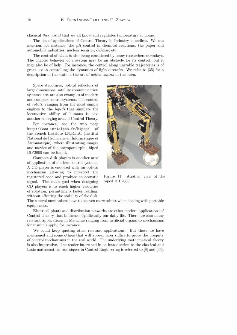
Figure 10: The bipedBIP2000.
Indeed, the range of applications of ControlTheory goes from the simplest mechanismswe manipulate in everyday life to the mostsophisticated ones, emerging in new technologies.
The book edited by W.S. Levine [26] providesa rather complete description of this variety ofapplications.
One of the simplest applications of ControlTheory appears in such an apparently simplemachine as the tank of our bathroom. Thereare many variants of tanks and some of thelicences go back to 1886 and can be foundin [25]. But all them work under the samebasic principles: the tank is supplied of regulatingvalves, security mechanisms that start the controlprocess, feedback mechanisms that provide moreor less water to the tank depending of the level ofwater in its interior and, finally, mechanisms thatavoid the unpleasant flooding in case that someof the other components fail.
The systems of heating, ventilation and airconditioning in big buildings are also very efficient
large scale control systems composed of interconnected thermo-fluid and electro-mechanical subsystems. The main goal of these systems is to keep a comfortableand good quality air under any circumstance, with a low operational cost anda high degree of reliability. The relevance of a proper and efficient functioningof these systems is crucial from the viewpoint of the impact in Economical andEnvironmental Sciences. The predecessor of these sophisticated systems is the
18 E. Fernandez-Cara and E. Zuazua
classical thermostat that we all know and regulates temperature at home.The list of applications of Control Theory in Industry is endless. We can
mention, for instance, the pH control in chemical reactions, the paper andautomobile industries, nuclear security, defense, etc.
The control of chaos is also being considered by many researchers nowadays.The chaotic behavior of a system may be an obstacle for its control; but itmay also be of help. For instance, the control along unstable trajectories is ofgreat use in controlling the dynamics of fight aircrafts. We refer to [35] for adescription of the state of the art of active control in this area.
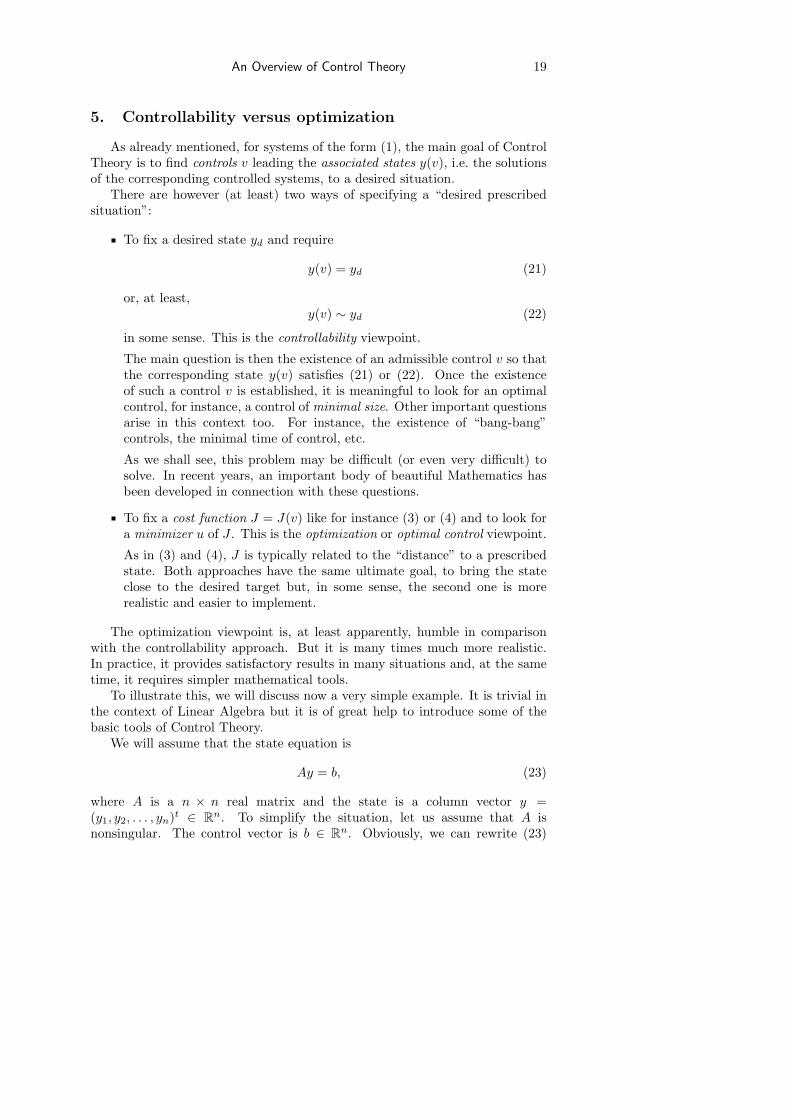
Figure 11: Another view of thebiped BIP2000.
Space structures, optical reflectors oflarge dimensions, satellite communicationsystems, etc. are also examples of modernand complex control systems. The controlof robots, ranging from the most simpleengines to the bipeds that simulate thelocomotive ability of humans is alsoanother emerging area of Control Theory.
For instance, see the web pagehttp://www.inrialpes.fr/bipop/ ofthe French Institute I.N.R.I.A. (InstitutNational de Recherche en Informatique etAutomatique), where illustrating imagesand movies of the antropomorphic bipedBIP2000 can be found.
Compact disk players is another areaof application of modern control systems.A CD player is endowed with an opticalmechanism allowing to interpret theregistered code and produce an acousticsignal. The main goal when designingCD players is to reach higher velocitiesof rotation, permitting a faster reading,without affecting the stability of the disk.The control mechanisms have to be even more robust when dealing with portableequipments.
Electrical plants and distribution networks are other modern applications ofControl Theory that influence significantly our daily life. There are also manyrelevant applications in Medicine ranging from artificial organs to mechanismsfor insulin supply, for instance.
We could keep quoting other relevant applications. But those we havementioned and some others that will appear later suffice to prove the ubiquityof control mechanisms in the real world. The underlying mathematical theoryis also impressive. The reader interested in an introduction to the classical andbasic mathematical techniques in Control Engineering is referred to [8] and [36].
An Overview of Control Theory 19
5. Controllability versus optimization
As already mentioned, for systems of the form (1), the main goal of ControlTheory is to find controls v leading the associated states y(v), i.e. the solutionsof the corresponding controlled systems, to a desired situation.
There are however (at least) two ways of specifying a “desired prescribedsituation”:
To fix a desired state yd and require
y(v) = yd (21)
or, at least,y(v) ∼ yd (22)
in some sense. This is the controllability viewpoint.
The main question is then the existence of an admissible control v so thatthe corresponding state y(v) satisfies (21) or (22). Once the existenceof such a control v is established, it is meaningful to look for an optimalcontrol, for instance, a control of minimal size. Other important questionsarise in this context too. For instance, the existence of “bang-bang”controls, the minimal time of control, etc.
As we shall see, this problem may be difficult (or even very difficult) tosolve. In recent years, an important body of beautiful Mathematics hasbeen developed in connection with these questions.
To fix a cost function J = J(v) like for instance (3) or (4) and to look fora minimizer u of J . This is the optimization or optimal control viewpoint.
As in (3) and (4), J is typically related to the “distance” to a prescribedstate. Both approaches have the same ultimate goal, to bring the stateclose to the desired target but, in some sense, the second one is morerealistic and easier to implement.
The optimization viewpoint is, at least apparently, humble in comparisonwith the controllability approach. But it is many times much more realistic.In practice, it provides satisfactory results in many situations and, at the sametime, it requires simpler mathematical tools.
To illustrate this, we will discuss now a very simple example. It is trivial inthe context of Linear Algebra but it is of great help to introduce some of thebasic tools of Control Theory.
We will assume that the state equation is
Ay = b, (23)
where A is a n × n real matrix and the state is a column vector y =(y1, y2, . . . , yn)t ∈ Rn. To simplify the situation, let us assume that A isnonsingular. The control vector is b ∈ Rn. Obviously, we can rewrite (23)
20 E. Fernandez-Cara and E. Zuazua
in the form y = A−1b, but we do not want to do this. In fact, we are mainlyinterested in those cases in which (23) can be difficult to solve.
Let us first adopt the controllability viewpoint. To be specific, let us imposeas an objective to make the first component y1 of y coincide with a prescribedvalue y∗1 :
y1 = y∗1 . (24)
This is the sense we are giving to (22) in this particular case. So, we are considerthe following controllability problem:
PROBLEM 0: To find b ∈ Rn such that the solution of (23) satisfies(24).
Roughly speaking, we are addressing here a partial controllability problem,in the sense that we are controlling only one component, y1 , of the state.
Obviously, such controls b exist. For instance, it suffices to take y∗ =(y∗1 , 0, · · · , 0)t and then choose b = Ay∗. But this argument, by means ofwhich we find the state directly without previously determining the control, isfrequently impossible to implement in practice. Indeed, in most real problems,we have first to find the control and, only then, we can compute the state bysolving the state equation.
The number of control parameters (the n components of b) is greater or equalthan the number of state components we have to control. But, what happensif we stress our own possibilities ? What happens if, for instance, b1, . . . , bn−1
are fixed and we only have at our disposal bn to control the system ?From a mathematical viewpoint, the question can be formulated as follows.
In this case,Ay = c + be (25)
where c ∈ Rn is a prescribed column vector, e is the unit vector (0, . . . , 0, 1)t
and b is a scalar control parameter. The corresponding controllability problemis now the following:
PROBLEM 1: To find b ∈ R such that the solution of (25) satisfies(24).
This is a less obvious question. However, it is not too difficult to solve. Notethat the solution y to (25) can be decomposed in the following way:
y = x + z, (26)
wherex = A−1c (27)
and z satisfiesAz = be, i.e. z = bz∗ z∗ = A−1e. (28)
To guarantee that y1 can take any value in R, as we have required in (24),it is necessary and sufficient to have z∗1 6= 0, z∗1 being the first component ofz∗ = A−1e.
In this way, we have a precise answer to this second controllability problem:
An Overview of Control Theory 21
The problem above can be solved for any y∗1 if and only if the firstcomponent of A−1e does not vanish.
Notice that, when the first component of A−1e vanishes, whatever the controlb is, we always have y1 = x1 , x1 being the first component of the fixed vector xin (27). In other words, y1 is not sensitive to the control bn . In this degeneratecase, the set of values taken by y1 is a singleton, a 0-dimensional manifold. Thus,we see that the state is confined in a “space” of low dimension and controllabilityis lost in general.
But, is it really frequent in practice to meet degenerate situations like theprevious one, where some components of the system are insensitive to thecontrol ?
Roughly speaking, it can be said that systems are generically not degenerate.In other words, in examples like the one above, it is actually rare that z∗1vanishes.
There are however a few remarks to do. When z∗1 does not vanish but is verysmall, even though controllability holds, the control process is very unstable inthe sense that one needs very large controls in order to get very small variationsof the state. In practice, this is very important and must be taken into account(one needs the system not only to be controllable but this to happen withrealistic and feasible controls).
On the other hand, it can be easily imagined that, when systems underconsideration are complex, i.e. many parameters are involved, it is difficultto know a priori whether or not there are components of the state that areinsensitive to the control1.
Let us now turn to the optimization approach. Let us see that the difficultieswe have encountered related to the possible degeneracy of the system disappear(which confirms the fact that this strategy leads to easier questions).
For example, let us assume that k > 0 is a reasonable bound of the controlb that we can apply. Let us put
J(bn) =12|y1 − y∗1 |2 ∀bn ∈ R, (29)
where y1 is the first component of the solution to (25). Then, it is reasonable toadmit that the best response is given by the solution to the following problem:
PROBLEM 1′: To find bkn ∈ [−k, k] such that
J(bkn) ≤ J(bn) ∀bn ∈ [−k, k]. (30)
Since bn 7→ J(bn) is a continuous function, it is clear that this problempossesses a solution bk
n ∈ Ik for each k > 0. This confirms that the consideredoptimal control problem is simpler.
1In fact, it is a very interesting and non trivial task to design strategies guaranteeing thatwe do not fall in a degenerate situation.
22 E. Fernandez-Cara and E. Zuazua
On the other hand, this point of view is completely natural and agrees withcommon sense. According to our intuition, most systems arising in real lifeshould possess an optimal strategy or configuration. At this respect L. Eulersaid:
“Universe is the most perfect system, designed by the most wiseCreator. Nothing will happen without emerging, at some extent, amaximum or minimum principle”.
Let us analyze more closely the similarities and differences arising in the twoprevious formulations of the control problem.
Assume the controllability property holds, that is, PROBLEM 1 is solvablefor any y∗1 . Then, if the target y∗1 is given and k is sufficiently large, thesolution to PROBLEM 1′ coincides with the solution to PROBLEM 1.
On the other hand, when there is no possibility to attain y∗1 exactly, theoptimization viewpoint, i.e. PROBLEM 1′, furnishes the best response.
To investigate whether the controllability property is satisfied, it can beappropriate to solve PROBLEM 1′ for each k > 0 and analyze the behaviorof the cost
Jk = minbn∈[−k,k]
J(bn) (31)
as k grows to infinity. If Jk stabilizes near a positive constant as k grows,we can suspect that y∗1 cannot be attained exactly, i.e. that PROBLEM 1does not have a solution for this value of y∗1 .
In view of these considerations, it is natural to address the questionof whether it is actually necessary to solve controllability problems likePROBLEM 1 or, by the contrary, whether solving a related optimal controlproblem (like PROBLEM 1′) suffices.
There is not a generic and systematic answer to this question. It depends onthe level of precision we require to the control process and this depends heavilyon the particular application one has in mind. For instance, when thinkingof technologies used to stabilize buildings, or when controlling space vehicles,etc., the efficiency of the control that is required demands much more thansimply choosing the best one with respect to a given criterion. In those cases, itis relevant to know how close the control will drive the state to the prescribedtarget. There are, consequently, a lot of examples for which simple optimizationarguments as those developed here are insufficient.
In order to choose the appropriate control we need first to develop a rigorousmodelling (in other words, we have to put equations to the real life system).The choice of the control problem is then a second relevant step in modelling.
Let us now recall and discuss some mathematical techniques allowing tohandle the minimization problems arising in the optimization approach (in fact,we shall see that these techniques are also relevant when the controllability pointof view is adopted).
An Overview of Control Theory 23
These problems are closely related to the Calculus of Variations. Here, wedo not intend to provide a survey of the techniques in this field but simply tomention some of the most common ideas.
For clarity, we shall start discussing Mathematical Programming. In thecontext of Optimization, Programming is not the art of writing computer codes.It was originated by the attempt to optimize the planning of the various tasksor activities in an organized system (a plant, a company, etc.). The goal is thento find what is known as an optimal planning or optimal programme.
The simplest problem of assignment suffices to exhibit the need of amathematical theory to address these issues.
Assume that we have 70 workers in a plant. They have differentqualifications and we have to assign them 70 different tasks. The total numberof possible distributions is 70 ! , which is of the order of 10100. Obviously, inorder to be able to solve rapidly a problem like this, we need a mathematicaltheory to provide a good strategy.
This is an example of assignment problem. Needless to say, problems ofthis kind are not only of academic nature, since they appear in most humanactivities.
In the context of Mathematical Programming, we first find linearprogramming techniques. As their name indicates, these are concerned withthose optimization problems in which the involved functional is linear.
Linear Programming was essentially unknown before 1947, even thoughJoseph Fourier had already observed in 1823 the relevance of the questions itdeals with. L.V. Kantorovich, in a monograph published in 1939, was the firstto indicate that a large class of different planning problems could be coveredwith the same formulation. The method of simplex, that we will recall below,was introduced in 1947 and its efficiency turned out to be so impressive thatvery rapidly it became a common tool in Industry.
There has been a very intense research in these topics that goes beyondLinear Programming and the method of simplex. We can mention for instancenonlinear programming methods, inspired by the method of descent. Thiswas formally introduced by the French mathematician A.L. Cauchy in theXIX Century. It relies on the idea of solving a nonlinear equation by searchingthe critical points of the corresponding primitive function.
Let us now give more details on Linear Programming. At this point, we willfollow a presentation similar to the one by G. Strang in [47].
The problems that one can address by means of linear programming involvethe minimization of linear functions subject to linear constraints. Althoughthey seem extremely simple, they are ubiquitous and can be applied in a largevariety of areas such as the control of traffic, Game Theory, Economics, etc.Furthermore, they involve in practice a huge quantity of unknowns, as in thecase of the optimal planning problems we have presented before.
The simplest problem in this field can be formulated in the following way:
Given a real matrix A of order M × N (with M ≤ N), and givena column vector b of M components and a column vector c with N
24 E. Fernandez-Cara and E. Zuazua
components, to minimize the linear function
〈c, x〉 = c1x1 + · · ·+ cNxN
under the restrictions
Ax = b, x ≥ 0.
Here and in the sequel, we use 〈· , ·〉 to denote the usual Euclidean scalarproducts in RN and RM . The associated norm will be denoted by | · |.
Of course, the second restriction has to be understood in the following way:
xj ≥ 0, j = 1, . . . , N.
In general, the solution to this problem is given by a unique vector x with theproperty that N −M components vanish. Accordingly, the problem consists infinding out which are the N −M components that vanish and, then, computingthe values of the remaining M components.
The method of simplex leads to the correct answer after a finite number ofsteps. The procedure is as follows:
• Step 1: We look for a vector x with N−M zero components and satisfyingAx = b, in addition to the unilateral restriction x ≥ 0. Obviously, thisfirst choice of x will not provide the optimal answer in general.
• Step 2: We modify appropriately this first choice of x allowing one ofthe zero components to become positive and vanishing one of the positivecomponents and this in such a way that the restrictions Ax = b and x ≥ 0are kept.
After a finite number of steps like Step 2, the value of 〈c, x〉 will have beentested at all possible minimal points. Obviously, the solution to the problem isobtained by choosing, among these points x, that one at which the minimumof 〈c, x〉 is attained.
Let us analyze the geometric meaning of the simplex method with anexample.
Let us consider the problem of minimizing the function
10x1 + 4x2 + 7x3
under the constraints
2x1 + x2 + x3 = 1, x1 , x2 , x3 ≥ 0.
In this case, the set of admissible triplets (x1 , x2 , x3), i.e. those satisfyingthe constraints is the triangle in R3 of vertices (0, 0, 1), (0, 1, 0) and (1/2, 0, 0)(a face of a tetrahedron). It is easy to see that the minimum is achieved at(0, 1, 0), where the value is 4.
An Overview of Control Theory 25
Let us try to give a geometrical explanation to this fact. Since x1 , x2 , x3 ≥ 0for any admissible triplet, the minimum of the function 10x1 + 4x2 + 7x3 hasnecessarily to be nonnegative. Moreover, the minimum cannot be zero since thehyperplane
10x1 + 4x2 + 7x3 = 0
has an empty intersection with the triangle of admissible states. Whenincreasing the cost 10x1 + 4x2 + 7x3 , i.e. when considering level sets of theform 10x1 + 4x2 + 7x3 = c with increasing c > 0, we are considering planesparallel to 10x1 + 4x2 + 7x3 = 0 that are getting away from the origin andcloser to the triangle of admissible states. The first value of c for which thelevel set intersects the admissible triangle provides the minimum of the costfunction and the point of contact is the minimizer.
It is immediate that this point is the vertex (0, 1, 0).These geometrical considerations indicate the relevance of the convexity of
the set where the minimum is being searched. Recall that, in a linear space E,a set K is convex if it satisfies the following property:
x, y ∈ K, λ ∈ [0, 1] ⇒ λx + (1− λ)y ∈ K.
The crucial role played by convexity will be also observed below, whenconsidering more sophisticated problems.
The method of simplex, despite its simplicity, is very efficient. There aremany variants, adapted to deal with particular problems. In some of them, whenlooking for the minimum, one runs across the convex set and not only alongits boundary. For instance, this is the case of Karmakar’s method, see [47].For more information on Linear Programming, the method of simplex and itsvariants, see for instance [40].
As the reader can easily figure out, many problems of interest inMathematical Programming concern the minimization of nonlinear functions.At this respect, let us recall the following fundamental result whose proof is thebasis of the so called Direct Method of the Calculus of Variations (DMCV):
Theorem 1 If H is a Hilbert space with norm ‖·‖H and the function J : H 7→ Ris continuous, convex and coercive in H, i.e. it satisfies
J(v) → +∞ as ‖v‖H → +∞, (32)
then J attains its minimum at some point u ∈ H. If, moreover, J is strictlyconvex, this point is unique.
If, in the previous result, J is a C1 function, any minimizer u necessarilysatisfies
J ′(u) = 0, u ∈ H. (33)
Usually, (33) is known as the Euler equation of the minimization problem
Minimize J(v) subject to v ∈ H. (34)
26 E. Fernandez-Cara and E. Zuazua
Consequently, if J is C1, Theorem 1 serves to prove that the (generallynonlinear) Euler equation (33) possesses at least one solution.
Many systems arising in Continuum Mechanics can be viewed as the Eulerequation of a minimization problem. Conversely, one can associate Eulerequations to many minimization problems. This mutual relation can be used inboth directions: either to solve differential equations by means of minimizationtechniques, or to solve minimization problems through the corresponding Eulerequations.
In particular, this allows proving existence results of equilibriumconfigurations for many problems in Continuum Mechanics.
Furthermore, combining these ideas with the approximation of the space Hwhere the minimization problem is formulated by means of finite dimensionalspaces and increasing the dimension to cover in the limit the whole space H, oneobtains Galerkin’s approximation method. Suitable choices of the approximatingsubspaces lead to the finite element methods.
In order to illustrate these statements and connect them to Control Theory,let us consider the example
x = Ax + Bv, t ∈ [0, T ],x(0) = x0,
(35)
in which the state x = (x1(t), . . . , xN (t))t is a vector in RN depending on t(the time variable) and the control v = (v1(t), . . . , vM (t))t is a vector with Mcomponents that also depends on time.
In (35), we will assume that A is a square, constant coefficient matrix ofdimension N ×N , so that the underlying system is autonomous, i.e. invariantwith respect to translations in time. The matrix B has also constant coefficientsand dimension N ×M .
Let us set
J(v) =12|x(T )− x1|2 +
µ
2
∫ T
0
|v(t)|2 dt ∀v ∈ L2(0, T ;RM ), (36)
where x1 ∈ RN is given, x(T ) is the final value of the solution of (35) and µ > 0.It is not hard to prove that J : L2(0, T ;RM ) 7→ R is well defined, continuous,
coercive and strictly convex. Consequently, J has a unique minimizer inL2(0, T ;RM ). This shows that the control problem (35)–(36) has a uniquesolution.
With the DMCV, the existence of minimizers for a large class of problemscan be proved. But there are many other interesting problems that do not enterin this simple framework, for which minimizers do not exist.
Indeed, let us consider the simplest and most classical problem in theCalculus of Variations: to show that the shortest path between two given pointsis the straight line segment.
Of course, it is very easy to show this by means of geometric arguments.However,
An Overview of Control Theory 27
What happens if we try to use the DMCV ?
The question is now to minimize the functional
∫ 1
0
|x(t)| dt
in the class of curves x : [0, 1] 7→ R2 such that x(0) = P and x(1) = Q, whereP and Q are two given points in the plane.
The natural functional space for this problem is not a Hilbert space. It canbe the Sobolev space W 1,1(0, 1) constituted by all functions x = x(t) such that xand its time derivative x belong to L1(0, 1). It can also be the more sophisticatedspace BV (0, 1) of functions of bounded variation. But these are not Hilbertspaces and solving the problem in any of them, preferably in BV (0, 1), becomesmuch more subtle.
We have described the DMCV in the context of problems withoutconstraints. Indeed, up to now, the functional has been minimized in thewhole space. But in most realistic situations the nature of the problem imposesrestrictions on the control and/or the state. This is the case for instance for thelinear programming problems we have considered above.
As we mentioned above, convexity plays a key role in this context too:
Theorem 2 Let H be a Hilbert space, K ⊂ H a closed convex set andJ : K 7→ R a convex continuous function. Let us also assume that eitherK is bounded or J is coercive in K, i.e.
J(v) → +∞ asv ∈ K, ‖v‖H → +∞.
Then, there exists a point u ∈ K where J reaches its minimum over K.Furthermore, if J is strictly convex, the minimizer is unique.
In order to illustrate this result, let us consider again the system (35) andthe functional
J(v) =12|x(T )− x1|2 +
µ
2
∫ T
0
|v(t)|2 dt ∀v ∈ K, (37)
where µ ≥ 0 and K ⊂ L2(0, T ;RM ) is a closed convex set. In view of Theorem 2,we see that, if µ > 0, the optimal control problem determined by (35) and (37)has a unique solution. If µ = 0 and K is bounded, this problem possesses atleast one solution.
Let us discuss more deeply the application of these techniques to the analysisof the control properties of the linear finite dimensional system (35).
Let J : H 7→ R be, for instance, a functional of class C1. Recall again that,at each point u where J reaches its minimum, one has
J ′(u) = 0, u ∈ H. (38)
28 E. Fernandez-Cara and E. Zuazua
It is also true that, when J is convex and C1, if u solves (38) then u is a globalminimizer of J in H. Equation (38) is the Euler equation of the correspondingminimization problem.
More generally, in a convex minimization problem, if the function to beminimized is of class C1, an Euler inequality is satisfied by each minimizer.Thus, u is a minimizer of the convex functional J in the convex set K of theHilbert space H if and only if
(J ′(u), v − u)H ≥ 0 ∀v ∈ K, u ∈ K. (39)
Here, (· , ·)H stands for the scalar product in H.In the context of Optimal Control, this characterization of u can be used
to deduce the corresponding optimality conditions, also called the optimalitysystem.
For instance, this can be made in the case of problem (35),(37). Indeed, itis easy to see that in this case (39) reduces to
µ
∫ T
0
〈u(t), v(t)− u(t)〉 dt + 〈x(T )− x1, zv(T )− zu(T )〉 ≥ 0
∀v ∈ K, u ∈ K,
(40)
where, for each v ∈ L2(0, T ;RM ), zv = zv(t) is the solution of
zv = Azv + Bv, t ∈ [0, T ],zv(0) = 0
(recall that 〈· , ·〉 stands for the Euclidean scalar products in RM and RN ).Now, let p = p(t) be the solution of the backward in time differential problem
−p = Atp, t ∈ [0, T ],p(T ) = x(T )− x1.
(41)
Then
〈x(T )−x1, zv(T )−zu(T )〉 = 〈p(T ), zv(T )−zu(T )〉 =∫ T
0
〈p(t), B(v(t)−u(t))〉 dt
and (40) can also be written in the form:
∫ T
0
〈µu(t) + Btp(t), v(t)− u(t)〉 dt ≥ 0
∀v ∈ K, u ∈ K.
(42)
The system constituted by the state equation (35) for v = u, i.e.
x = Ax + Bu, t ∈ [0, T ],x(0) = x0,
(43)
An Overview of Control Theory 29
the adjoint state equation (41) and the inequalities (42) is referred to as theoptimality system. This system provides, in the case under consideration, acharacterization of the optimal control.
The function p = p(t) is the adjoint state. As we have seen, the introductionof p leads to a rewriting of (40) that is more explicit and easier to handle.
Very often, when addressing optimization problems, we have to deal withrestrictions or constraints on the controls and/or state. Lagrange multipliersthen play a fundamental role and are needed in order to write the equationssatisfied by the minimizers: the so called Euler-Lagrange equations.
To do that, we must introduce the associated Lagrangian and, then, wemust analyze its saddle points. The determination of saddle points leads to twoequivalent extremal problems of dual nature.
This is a surprising fact in this theory that can be often used with efficiency:the original minimization problem being difficult to solve, one may often writea dual minimization problem (passing through the Lagrangian); it may wellhappen to the second problem to be simpler than the original one.
Saddle points arise naturally in many optimization problems. But they canalso be viewed as the solutions of minimax problems. Minimax problems arisein many contexts, for instance:
• In Differential Game Theory, where two or more players compete tryingto maximize their profit and minimize the one of the others.
• In the characterization of the proper vibrations of elastic bodies. Indeed,very often these can be characterized as eigenvalues of a self-adjointcompact operator in a Hilbert space through a minimax principle relatedto the Rayleigh quotient.
One of the most relevant contributions in this field was the one byJ. Von Neumann in the middle of the XX Century, proving that the existenceof a minimax is guaranteed under very weak conditions.
In the last three decades, these results have been used systematically forsolving nonlinear differential problems, in particular with the help of theMountain Pass Lemma (for instance, see [20]). At this respect, it is worthmentioning that a mountain pass is indeed a beautiful example of saddle pointprovided by Nature. A mountain pass is the location one chooses to crossa mountain chain: this point must be of minimal height along the mountainchain but, on the contrary, it is of maximal height along the crossing path wefollow.
The reader interested in learning more about Convex Analysis and therelated duality theory is referred to the books [9] and [41], by I. Ekelandand R. Temam and R.T. Rockafellar, respectively. The lecture notes byB. Larrouturou and P.L. Lions [23] contain interesting introductions to theseand other related topics, like mathematical modelling, the theory of partialdifferential equations and numerical approximation techniques.
30 E. Fernandez-Cara and E. Zuazua
6. Controllability of linear finite dimensional systems
We will now be concerned with the controllability of ordinary differentialequations. We will start by considering linear systems.
As we said above, Control Theory is full of interesting mathematicalresults that have had a tremendous impact in the world of applications (mostof them are too complex to be reproduced in these notes). One of theseimportant results, simple at the same time, is a theorem by R.E. Kalman whichcharacterizes the linear systems that are controllable.
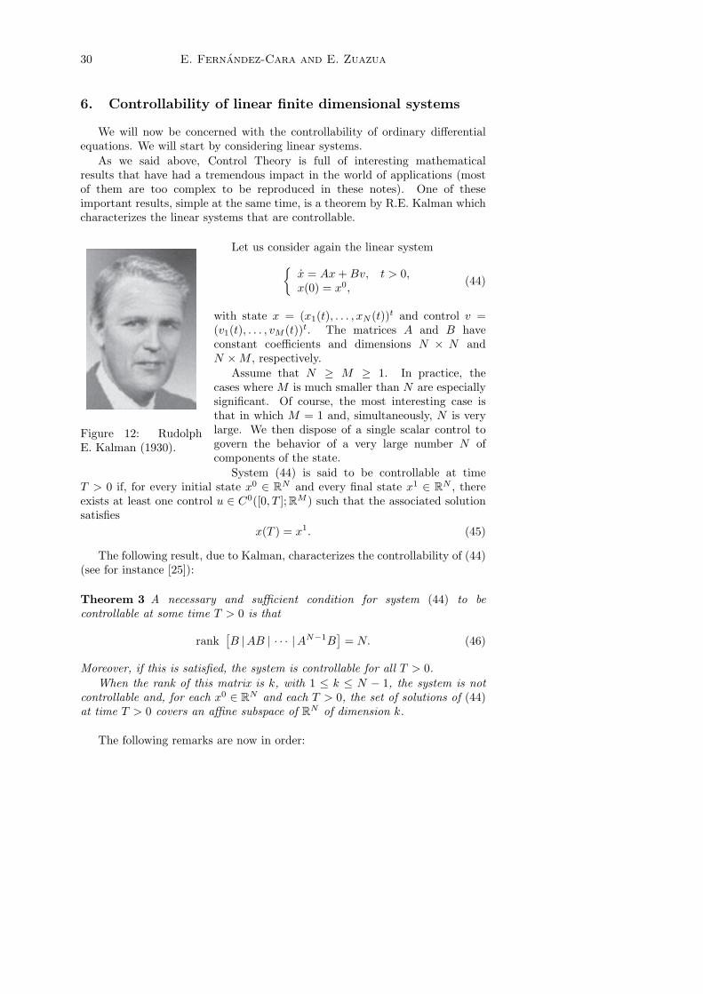
Figure 12: RudolphE. Kalman (1930).
Let us consider again the linear system
x = Ax + Bv, t > 0,x(0) = x0,
(44)
with state x = (x1(t), . . . , xN (t))t and control v =(v1(t), . . . , vM (t))t. The matrices A and B haveconstant coefficients and dimensions N × N andN ×M , respectively.
Assume that N ≥ M ≥ 1. In practice, thecases where M is much smaller than N are especiallysignificant. Of course, the most interesting case isthat in which M = 1 and, simultaneously, N is verylarge. We then dispose of a single scalar control togovern the behavior of a very large number N ofcomponents of the state.
System (44) is said to be controllable at timeT > 0 if, for every initial state x0 ∈ RN and every final state x1 ∈ RN , thereexists at least one control u ∈ C0([0, T ];RM ) such that the associated solutionsatisfies
x(T ) = x1. (45)
The following result, due to Kalman, characterizes the controllability of (44)(see for instance [25]):
Theorem 3 A necessary and sufficient condition for system (44) to becontrollable at some time T > 0 is that
rank[B |AB | · · · |AN−1B
]= N. (46)
Moreover, if this is satisfied, the system is controllable for all T > 0.When the rank of this matrix is k, with 1 ≤ k ≤ N − 1, the system is not
controllable and, for each x0 ∈ RN and each T > 0, the set of solutions of (44)at time T > 0 covers an affine subspace of RN of dimension k.
The following remarks are now in order:

An Overview of Control Theory 31
• The degree of controllability of a system like (44) is completely determinedby the rank of the corresponding matrix in (46). This rank indicates howmany components of the system are sensitive to the action of the control.
• The matrix in (46) is of dimension (N ×M) ×N so that, when we onlyhave one control at our disposal (i.e. M = 1), this is a N ×N matrix. Itis obviously in this case when it is harder to the rank of this matrix to beN . This is in agreement with common sense, since the system should beeasier to control when the number of controllers is larger.
• The system is controllable at some time if and only if it is controllable atany positive time. In some sense, this means that, in (44), informationpropagates at infinite speed. Of course, this property is not true in generalin the context of partial differential equations.
As we mentioned above, the concept of adjoint system plays an importantrole in Control Theory. In the present context, the adjoint system of (44) is thefollowing: −ϕ = Atϕ, t < T,
ϕ(T ) = ϕ0.(47)
Let us emphasize the fact that (47) is a backward (in time) system. Indeed,in (47) the sense of time has been reversed and the differential system has beencompleted with a final condition at time t = T .
The following result holds:
Theorem 4 The rank of the matrix in (46) is N if and only if, for every T > 0,there exists a constant C(T ) > 0 such that
|ϕ0|2 ≤ C(T )∫ T
0
|Btϕ|2 dt (48)
for every solution of (47).
The inequality (48) is called an observability inequality. It can be viewed asthe dual version of the controllability property of system (44).
This inequality guarantees that the adjoint system can be “observed”through Btϕ, which provides M linear combinations of the adjoint state. When(48) is satisfied, we can affirm that, from the controllability viewpoint, Bt
captures appropriately all the components of the adjoint state ϕ. This turnsout to be equivalent to the controllability of (44) since, in this case, the controlu acts efficiently through the matrix B on all the components of the state x.
Inequalities of this kind play also a central role in inverse problems, wherethe goal is to reconstruct the properties of an unknown (or only partiallyknown) medium or system by means of partial measurements. The observabilityinequality guarantees that the measurements Btϕ are sufficient to detect all thecomponents of the system.
32 E. Fernandez-Cara and E. Zuazua
The proof of Theorem 4 is quite simple. Actually, it suffices to write thesolutions of (44) and (47) using the variation of constants formula and, then, toapply the Cayley-Hamilton theorem, that guarantees that any matrix is a rootof its own characteristic polynomial.
Thus, to prove that (46) implies (48), it is sufficient to show that, when (46)is true, the mapping
ϕ0 7→(∫ T
0
|Btϕ|2 dt
)1/2
is a norm in RN . To do that, it suffices to check that the following uniquenessor unique continuation result holds:
If Btϕ = 0 for 0 ≤ t ≤ T then, necessarily, ϕ ≡ 0.
It is in the proof of this result that the rank condition is needed.Let us now see how, using (48), we can build controls such that the
associated solutions to (44) satisfy (45). This will provide another idea of howcontrollability and optimal control problems are related.
Given initial and final states x0 and x1 and a control time T > 0, let usconsider the quadratic functional I, with
I(ϕ0) =12
∫ T
0
|Btϕ|2 dt− 〈x1, ϕ0〉+ 〈x0, ϕ(0)〉 ∀ϕ0 ∈ RN , (49)
where ϕ is the solution of the adjoint system (47) associated to the final stateϕ0.
The function ϕ0 7→ I(ϕ0) is strictly convex and continuous in RN . In viewof (48), it is also coercive, that is,
lim|ϕ0|→∞
I(ϕ0) = +∞. (50)
Therefore, I has a unique minimizer in RN , that we shall denote by ϕ0. Let uswrite the Euler equation associated to the minimization of the functional (49):
∫ T
0
〈Btϕ, Btϕ〉 dt− 〈x1, ϕ0〉+ 〈x0, ϕ(0)〉 = 0 ∀ϕ0 ∈ RN , ϕ0 ∈ RN . (51)
Here, ϕ is the solution of the adjoint system (47) associated to the final stateϕ0.
From (51), we deduce that u = Btϕ is a control for (44) that guaranteesthat (45) is satisfied. Indeed, if we denote by x the solution of (44) associatedto u, we have that
∫ T
0
〈Btϕ, Btϕ〉 dt = 〈x(T ), ϕ0〉 − 〈x0, ϕ(0)〉 ∀ϕ0 ∈ RN . (52)
Comparing (51) and (52), we see that the previous assertion is true.
An Overview of Control Theory 33
It is interesting to observe that, from the rank condition, we can deduceseveral variants of the observability inequality (48). In particular,
|ϕ0| ≤ C(T )∫ T
0
|Btϕ| dt (53)
This allows us to build controllers of different kinds.Indeed, consider for instance the functional Jbb , given by
Jbb(ϕ0) =12
(∫ T
0
|Btϕ| dt
)2
− 〈x1, ϕ0〉+ 〈x0, ϕ(0)〉 ∀ϕ0 ∈ RN . (54)
This is again strictly convex, continuous and coercive. Thus, it possesses exactlyone minimizer ϕ0
bb . Let us denote by ϕbb the solution of the correspondingadjoint system. Arguing as above, it can be seen that the new control ubb , with
ubb =
(∫ T
0
|Btϕbb| dt
)sgn(Btϕbb), (55)
makes the solution of (44) satisfy (45). This time, we have built a bang-bangcontrol, whose components can only take two values:
±∫ T
0
|Btϕbb| dt.
The control u that we have obtained minimizing J is the one of minimalnorm in L2(0, T ;RM ) among all controls guaranteeing (45). On the other hand,ubb is the control of minimal L∞ norm. The first one is smooth and the secondone is piecewise constant and, therefore, discontinuous in general. However, thebang-bang control is easier to compute and apply since, as we saw explicitlyin the case of the pendulum, we only need to determine its amplitude and thelocation of the switching points. Both controls u and ubb are optimal withrespect to some optimality criterium.
We have seen that, in the context of linear control systems, whencontrollability holds, the control may be computed by solving a minimizationproblem. This is also relevant from a computational viewpoint since it providesuseful ideas to design efficient approximation methods.
7. Controllability of nonlinear finite dimensional systems
Let us now discuss the controllability of some nonlinear control systems.This is a very complex topic and it would be impossible to describe in a fewpages all the significant results in this field. We will just recall some basic ideas.
When the goal is to produce small variations or deformations of the state,it might be sufficient to proceed using linearization arguments. More precisely,let us consider the system
x = f(x, u), t > 0,x(0) = x0,
(56)
34 E. Fernandez-Cara and E. Zuazua
where f : RN ×RM 7→ RN is smooth and f(0, 0) = 0. The linearized system atu = 0, x = 0 is the following:
x =∂f
∂x(0, 0)x +
∂f
∂u(0, 0)u, t > 0,
x(0) = 0.
(57)
Obviously, (57) is of the form (44), with
A =∂f
∂x(0, 0), B =
∂f
∂u(0, 0), x0 = 0. (58)
Therefore, the rank condition
rank [B|AB| · · · |AN−1B] = N (59)
is the one that guarantees the controllability of (57).Based on the inverse function theorem, it is not difficult to see that, if
condition (59) is satisfied, then (56) is locally controllable in the following sense:
For every T > 0, there exists a neighborhood BT of the origin inRN such that, for any initial and final states x0, x1 ∈ BT , thereexist controls u such that the associated solutions of the system (56)satisfy
x(T ) = x1 . (60)
However, this analysis is not sufficient to obtain results of global nature.A natural condition that can be imposed on the system (56) in order to
guarantee global controllability is that, at each point x0 ∈ RN , by choosing alladmissible controls u ∈ Uad , we can recover deformations of the state in all thedirections of RN . But,
Which are the directions in which the state x can be deformedstarting from x0 ?
Obviously, the state can be deformed in all directions f(x0, u) with u ∈ Uad .But these are not all the directions of RN when M < N . On the other hand,as we have seen in the linear case, there exist situations in which M < N and,at the same time, controllability holds thanks to the rank condition (59).
In the nonlinear framework, the directions in which the state may bedeformed around x0 are actually those belonging to the Lie algebra generatedby the vector fields f(x0, u), when u varies in the set of admissible controls Uad .Recall that the Lie algebra A generated by a family F of regular vector fieldsis the set of Lie brackets [f, g] with f, g ∈ F , where
[f, g] = (∇g)f − (∇f)g
and all the fields that can be obtained iterating this process of computing Liebrackets.
The following result can be proved (see [46]):
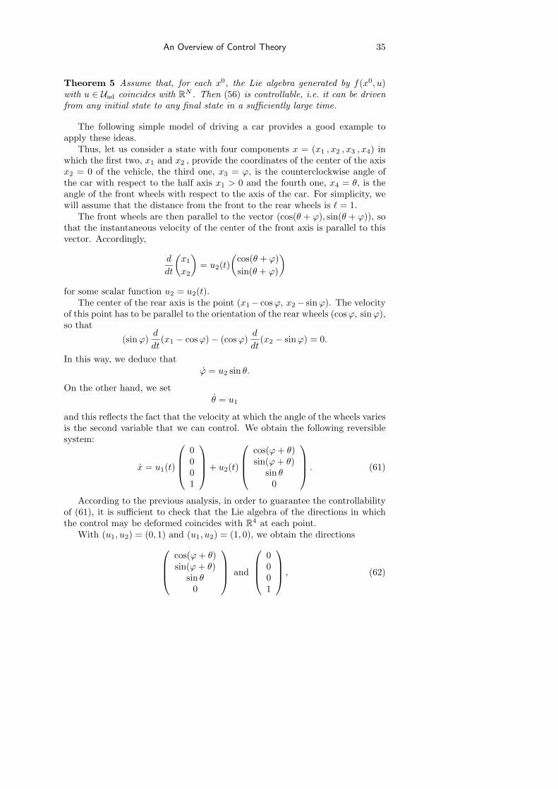
An Overview of Control Theory 35
Theorem 5 Assume that, for each x0, the Lie algebra generated by f(x0, u)with u ∈ Uad coincides with RN . Then (56) is controllable, i.e. it can be drivenfrom any initial state to any final state in a sufficiently large time.
The following simple model of driving a car provides a good example toapply these ideas.
Thus, let us consider a state with four components x = (x1 , x2 , x3 , x4) inwhich the first two, x1 and x2 , provide the coordinates of the center of the axisx2 = 0 of the vehicle, the third one, x3 = ϕ, is the counterclockwise angle ofthe car with respect to the half axis x1 > 0 and the fourth one, x4 = θ, is theangle of the front wheels with respect to the axis of the car. For simplicity, wewill assume that the distance from the front to the rear wheels is ` = 1.
The front wheels are then parallel to the vector (cos(θ + ϕ), sin(θ + ϕ)), sothat the instantaneous velocity of the center of the front axis is parallel to thisvector. Accordingly,
d
dt
(x1
x2
)= u2(t)
(cos(θ + ϕ)sin(θ + ϕ)
)
for some scalar function u2 = u2(t).The center of the rear axis is the point (x1− cos ϕ, x2− sin ϕ). The velocity
of this point has to be parallel to the orientation of the rear wheels (cosϕ, sinϕ),so that
(sinϕ)d
dt(x1 − cosϕ)− (cos ϕ)
d
dt(x2 − sin ϕ) = 0.
In this way, we deduce thatϕ = u2 sin θ.
On the other hand, we setθ = u1
and this reflects the fact that the velocity at which the angle of the wheels variesis the second variable that we can control. We obtain the following reversiblesystem:
x = u1(t)
0001
+ u2(t)
cos(ϕ + θ)sin(ϕ + θ)
sin θ0
. (61)
According to the previous analysis, in order to guarantee the controllabilityof (61), it is sufficient to check that the Lie algebra of the directions in whichthe control may be deformed coincides with R4 at each point.
With (u1, u2) = (0, 1) and (u1, u2) = (1, 0), we obtain the directions
cos(ϕ + θ)sin(ϕ + θ)
sin θ0
and
0001
, (62)
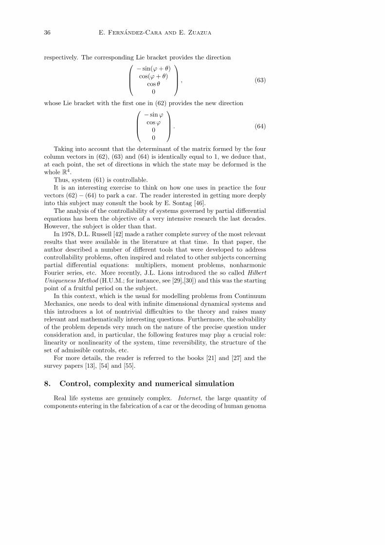
36 E. Fernandez-Cara and E. Zuazua
respectively. The corresponding Lie bracket provides the direction
− sin(ϕ + θ)cos(ϕ + θ)
cos θ0
, (63)
whose Lie bracket with the first one in (62) provides the new direction
− sin ϕcos ϕ
00
. (64)
Taking into account that the determinant of the matrix formed by the fourcolumn vectors in (62), (63) and (64) is identically equal to 1, we deduce that,at each point, the set of directions in which the state may be deformed is thewhole R4.
Thus, system (61) is controllable.It is an interesting exercise to think on how one uses in practice the four
vectors (62)− (64) to park a car. The reader interested in getting more deeplyinto this subject may consult the book by E. Sontag [46].
The analysis of the controllability of systems governed by partial differentialequations has been the objective of a very intensive research the last decades.However, the subject is older than that.
In 1978, D.L. Russell [42] made a rather complete survey of the most relevantresults that were available in the literature at that time. In that paper, theauthor described a number of different tools that were developed to addresscontrollability problems, often inspired and related to other subjects concerningpartial differential equations: multipliers, moment problems, nonharmonicFourier series, etc. More recently, J.L. Lions introduced the so called HilbertUniqueness Method (H.U.M.; for instance, see [29],[30]) and this was the startingpoint of a fruitful period on the subject.
In this context, which is the usual for modelling problems from ContinuumMechanics, one needs to deal with infinite dimensional dynamical systems andthis introduces a lot of nontrivial difficulties to the theory and raises manyrelevant and mathematically interesting questions. Furthermore, the solvabilityof the problem depends very much on the nature of the precise question underconsideration and, in particular, the following features may play a crucial role:linearity or nonlinearity of the system, time reversibility, the structure of theset of admissible controls, etc.
For more details, the reader is referred to the books [21] and [27] and thesurvey papers [13], [54] and [55].
8. Control, complexity and numerical simulation
Real life systems are genuinely complex. Internet, the large quantity ofcomponents entering in the fabrication of a car or the decoding of human genoma
An Overview of Control Theory 37
are good examples of this fact.The algebraic system (23) considered in Section 5 is of course academic
but it suffices by itself to show that not all the components of the state arealways sensitive to the chosen control. One can easily imagine how dramaticcan the situation be when dealing with complex (industrial) systems. Indeed,determining whether a given controller allows to act on all the components ofa system may be a very difficult task.
But complexity does not only arise for systems in Technology and Industry.It is also present in Nature. At this respect, it is worth recalling the followinganecdote. In 1526, the Spanish King “Alfonso X El Sabio” got into the Alcazarof Segovia after a violent storm and exclaimed:
“If God had consulted me when He was creating the world, I wouldhave recommended a simpler system.”
Recently we have learned about a great news, a historical achievement ofScience: the complete decoding of human genoma. The genoma code is a goodproof of the complexity which is intrinsic to life. And, however, one has not toforget that, although the decoding has been achieved, there will still be a lot todo before being able to use efficiently all this information for medical purposes.
Complexity is also closely related to numerical simulation. In practice,any efficient control strategy, in order to be implemented, has to go throughnumerical simulation. This requires discretizing the control system, which veryoften increases its already high complexity.
The recent advances produced in Informatics allow nowadays to usenumerical simulation at any step of an industrial project: conception,development and qualification. This relative success of numerical methodsin Engineering versus other traditional methods relies on the facts that theassociated experimental costs are considerably lower and, also, that numericalsimulation allows testing at the realistic scale, without the technical restrictionsmotivated by instrumentation.
This new scientific method, based on a combination of Mathematics andInformatics, is being seriously consolidated. Other Sciences are also closelyinvolved in this melting, since many mathematical models stem from them:Mechanics, Physics, Chemistry, Biology, Economics, etc. Thus, we are nowable to solve more sophisticated problems than before and the complexity ofthe systems we will be able to solve in the near future will keep increasing.Thanks in particular to parallelization techniques, the description and numericalsimulation of complex systems in an acceptable time is more and more feasible.
However, this panorama leads to significant and challenging difficulties thatwe are now going to discuss.
The first one is that, in practice, the systems under consideration are infact the coupling of several complex subsystems. Each of them has its owndynamics but the coupling may produce new and unexpected phenomena dueto their interaction.
An example of this situation is found in the mathematical description ofreactive fluids which are used, for instance, for the propulsion of spatial vehicles.
38 E. Fernandez-Cara and E. Zuazua
For these systems, one has to perform a modular analysis, separating andsimulating numerically each single element and, then, assembling the results.But this is a major task and much has still to be done2.
There are many relevant examples of complex systems for which coupling canbe the origin of important difficulties. In the context of Aerospatial Technology,besides the combustion of reactive fluids, we find fluid-structure interactionswhich are extremely important when driving the craft, because of the vibrationsoriginated by combustion. Other significant examples are weather predictionand Climatology, where the interactions of atmosphere, ocean, earth, etc. playa crucial role. A more detailed description of the present situation of researchand perspectives at this respect can be found in the paper [1], by J. Achacheand A. Bensoussan.
In our context, the following must be taken into account:
Only complex systems are actually relevant from the viewpoint ofapplications.
Furthermore, in order to solve a relevant problem, we must first identifythe various subsystems and the way they interact.
Let us now indicate some of the mathematical techniques that have beenrecently developed (and to some extent re-visited) to deal with complexity andperform the appropriate decomposition of large systems that we have mentionedas a need:
• The solution of linear systems.
When the linear system we have to solve presents a block-sparse structure,it is convenient to apply methods combining appropriately the localsolution of the subsystems corresponding to the individual blocks. This isa frequent situation when dealing with finite difference or finite elementdiscretizations of a differential system.
The most usual way to proceed is to introduce preconditioners, determinedby the solutions to the subsystems, each of them being computed withone processor and, then, to perform the global solution with parallelizediterative methods.
• Multigrid methods.
These are very popular today. Assume we are considering a linear systemoriginated by the discretization of a differential equation. The main idea ofa multigrid method is to “separate” the low and the high frequencies of thesolution in the computation procedure. Thus we compute approximationsof the solution at different levels, for instance working alternately with acoarse and a fine grid and incorporating adequate coupling mechanisms.
2To understand the level of difficulty, it is sufficient to consider a hybrid parabolic-hyperbolic system and try to match the numerical methods obtained with a finite differencemethod in the hyperbolic component and a finite element method in the parabolic one.
An Overview of Control Theory 39
The underlying reason is that any grid, even if it is very fine, is unable tocapture sufficiently high frequency oscillations, just as an ordinary watchis unable to measure microseconds.
• Domain decomposition methods.
Now, assume that (1) is a boundary value problem for a partial differentialequation in the N -dimensional domain Ω. If Ω has a complex geometricalstructure, it is very natural to decompose (1) in several similar systemswritten in simpler domains.
This can be achieved with domain decomposition techniques. The mainidea is to split Ω in the form
Ω = Ω1 ∪ Ω2 ∪ · · · ∪ Ωm , (65)
and to introduce then an iterative scheme based on computations on eachΩi separately.
Actually, this is not new. Some seminal ideas can be found in Volume IIof the book [7] by R. Courant and D. Hilbert. Since then, there havebeen lots of works on domain decomposition methods applied to partialdifferential systems (see for instance [24]). However, the role of thesemethods in the solution of control problems has not still been analyzedcompletely.
• Alternating direction methods.
Frequently, we have to consider models involving time-dependent partialdifferential equations in several space dimensions. After standard timediscretization, one is led at each time step to a set of (stationary) partialdifferential problems whose solution, in many cases, is difficult to achieve.
This is again connected to the need of decomposing complex systems inmore simple subsystems. These ideas lead to the methods of alternatingdirections, of great use in this context. A complete analysis can be foundin [51]. In the particular, but very illustrating context of the Navier-Stokesequations, these methods have been described for instance in [19] and [38].
However, from the viewpoint of Control Theory, alternating directionmethods have not been, up to now, sufficiently explored.
The interaction of the various components of a complex system is also adifficulty of major importance in control problems. As we mentioned above, forreal life control problems, we have first to choose an appropriate model and thenwe have also to make a choice of the control property. But necessarily one endsup introducing numerical discretization algorithms to make all this computable.Essentially, we will have to be able to compute an accurate approximation of thecontrol and this will be made only if we solve numerically a discretized controlproblem.
At this point, let us observe that, as mentioned in [53], some models obtainedafter discretization (for instance via the finite element method) are not only
40 E. Fernandez-Cara and E. Zuazua
relevant regarded as approximations of the underlying continuous models butalso by themselves, as genuine models of the real physical world3.
Let us consider a simple example in order to illustrate some extra, somehowunexpected, difficulties that the discretization may bring to the control process.
Consider again the state equation (1). To fix ideas, we will assume that ourcontrol problem is as follows
To find u ∈ Uad such that
Φ(u, y(u)) ≤ Φ(v, y(v)) ∀v ∈ Uad , (66)
where Φ = Φ(v, y) is a given function.
Then, we are led to the following crucial question:
What is an appropriate discretized control problem ?
There are at least two reasonable possible answers:
• First approximation method.
We first discretize Uad and (1) and obtain Uad,h and the new (discrete)state equation
Ah(yh) = f(vh). (67)
Here, h stands for a small parameter that measures the characteristicsize of the “numerical mesh”. Later, we let h → 0 to make the discreteproblem converge to the continuous one. If Uad,h and (67) are introducedthe right way, we can expect to obtain a “discrete state” yh(vh) for each“discrete admissible” control vh ∈ Uad,h .
Then, we search for an optimal control at the discrete level, i.e. a controluh ∈ Uad,h such that
Φ(uh, yh(uh)) ≤ Φ(vh, yh(vh)) ∀vh ∈ Uad,h . (68)
This corresponds to the following scheme:
MODEL −→ DISCRETIZATION −→ CONTROL.
Indeed, starting from the continuous control problem, we first discretize itand we then compute the control of the discretized model. This providesa first natural method for solving in practice the control problem.
3The reader can find in [53] details on how the finite element method was born around1960. In this article it is also explained that, since its origins, finite elements have been viewedas a tool to build legitimate discrete models for the mechanical systems arising in Nature andEngineering, as well as a method to approximate partial differential systems.
An Overview of Control Theory 41
• Second approximation method.
However, we can also do as follows. We analyze the original controlproblem (1),(66) and we characterize the optimal solution and controlin terms of an optimality system. We have already seen that, in practice,this is just to write the Euler or Euler-Lagrange equations associated tothe minimization problem we are dealing with. We have already describedhow optimality systems can be found for some particular control problems.
The optimality systems are of the form
A(y) = f(u), B(y)p = g(u, y) (69)
(where B(y) is a linear operator), together with an additional equationrelating u, y and p. To simplify our exposition, let us assume that thelatter can be written in the form
Q(u, y, p) = 0 (70)
for some mapping Q. The key point is that, if u, y and p solve theoptimality system (69) − (70), then u is an optimal control and y is theassociate state. Of course, p is the adjoint state associated to u and y.
Then, we can discretize and solve numerically (69),(70). This correspondsto a different approach:
MODEL −→ CONTROL −→ DISCRETIZATION.
Notice that, in this second approach, we have interchanged the controland discretization steps. Now, we first analyze the continuous controlproblem and, only later, we proceed to the numerical discretization.
It is not always true that these two methods provide the same results.For example, it is shown in [18] that, with a finite element approximation,
the first one may give erroneous results in vibration problems. This is connectedto the lack of accuracy of finite elements in the computation of high frequencysolutions to the wave equation, see [53]4.
On the other hand, it has been observed that, for the solution of a lot ofoptimal design problems, the first strategy is preferable; see for instance [34]and [37].
The commutativity of the DISCRETIZATION/CONTROL scheme is atpresent a subject that is not well understood and requires further investigation.We do not still have a significant set of results allowing to determine whenthese two approaches provide similar results and when they do not. Certainly,the answer depends heavily on the nature of the model under consideration.
4Nevertheless, the disagreement of these two methods may be relevant not only as a purelynumerical phenomenon but also at the level of modelling since, as we said above, in manyengineering applications discrete models are often directly chosen.
42 E. Fernandez-Cara and E. Zuazua
In this sense, control problems for elliptic and parabolic partial differentialequations, because of their intrinsic dissipative feature, will be better behavedthan hyperbolic systems. We refer the interested reader to [56] for a completeaccount of this fact. It is however expected that much progress will be made inthis context in the near future.
9. Two challenging applications
In this Section, we will mention two control problems whose solution willprobably play an important role in the context of applications in the near future.
9.1. Molecular control via laser technology
We have already said that there are many technological contexts whereControl Theory plays a crucial role. One of them, which has had a very recentdevelopment and announces very promising perspectives, is the laser control ofchemical reactions.
The basic principles used for the control of industrial processes in Chemistryhave traditionally been the same for many years. Essentially, the strategies havebeen (a) to introduce changes in the temperature or pressure in the reactionsand (b) to use catalyzers.
Laser technology, developed in the last four decades, is now playing anincreasingly important role in molecular design. Indeed, the basic principlesin Quantum Mechanics rely on the wave nature of both light and matter.Accordingly, it is reasonable to believe that the use of laser will be an efficientmechanism for the control of chemical reactions.
The experimental results we have at our disposal at present allow us toexpect that this approach will reach high levels of precision in the near future.However, there are still many important technical difficulties to overcome.
For instance, one of the greatest drawbacks is found when the moleculesare “not very isolated”. In this case, collisions make it difficult to define theirphases and, as a consequence, it is very hard to choose an appropriate choiceof the control. A second limitation, of a much more technological nature, isrelated to the design of lasers with well defined phases, not too sensitive to theinstabilities of instruments.
For more details on the modelling and technological aspects, the reader isreferred to the expository paper [4] by P. Brumer and M. Shapiro.
The goal of this subsection is to provide a brief introduction to themathematical problems one finds when addressing the control of chemicalreactions.
Laser control is a subject of high interest where Mathematics are notsufficiently developed. The models needed to describe these phenomena leadto complex (nonlinear) Schrodinger equations for which the results we are ableto deduce are really poor at present. Thus,
An Overview of Control Theory 43
We do not dispose at this moment of a complete theory for thecorresponding initial or iniial/boundary value problems.
Standard numerical methods are not sufficiently efficient and, accordingly,it is difficult to test the accuracy of the models that are by now available.
The control problems arising in this context are bilinear. This addsfundamental difficulties from a mathematical viewpoint and makes theseproblems extremely challenging. Indeed, we find here genuine nonlinearproblems for which, apparently, the existing linear theory is insufficient toprovide an answer in a first approach.
In fact, it suffices to analyze the most simple bilinear control problems wherewave phenomena appear to understand the complexity of this topic. Thus, letus illustrate this situation with a model concerning the linear one-dimensionalSchrodinger equation. It is clear that this is insufficient by itself to describe allthe complex phenomena arising in molecular control via laser technology. Butit suffices to present the main mathematical problem and difficulties arising inthis context.
The system is the following:
iφt + φxx + p(t)xφ = 0 0 < x < 1, 0 < t < T,φ(0, t) = φ(1, t) = 0, 0 < t < T,φ(x, 0) = φ0(x), 0 < x < 1.
(71)
In (71), φ = φ(x, t) is the state and p = p(t) is the control. Although φ iscomplex-valued, p(t) is real for all t. The control p can be interpreted as theintensity of an applied electrical field and x is the (prescribed) direction of thelaser.
The state φ = φ(x, t) is the wave function of the molecular system. Itcan be regarded as a function that furnishes information on the location of anelementary particle: for arbitrary a and b with 0 ≤ a < b ≤ 1, the quantity
P (a, b; t) =∫ b
a
|φ(x, t)|2 dx
can be viewed as the probability that the particle is located in (a, b) at time t.The controllability problem for (71) is to find the set of attainable states
φ(·, T ) at a final time T as p runs over the whole space L2(0, T ).It is worth mentioning that, contrarily to what happens to many other
control problems, the set of attainable states at time T depends strongly onthe initial data φ0. In particular, when φ0 = 0 the unique solution of (71) isφ ≡ 0 whatever p is and, therefore, the unique attainable state is φ(·, T ) ≡ 0. Itis thus clear that, if we want to consider a nontrivial situation, we must supposethat φ0 6= 0.
We say that this is a bilinear control problem, since the unique nonlinearity inthe model is the term p(t)xφ, which is essentially the product of the control andthe state. Although the nonlinearity might seem simple, this control problem
44 E. Fernandez-Cara and E. Zuazua
becomes rather complex and out of the scope of the existing methods in theliterature.
For an overview on the present state of the art of the control of systemsgoverned by the Schrodinger equation, we refer to the survey article [57] andthe references therein.
9.2. An environmental control problem
For those who live and work on the seaside or next to a river, the relevanceof being able to predict drastic changes of weather or on the state of the sea isobvious. In particular, it is vital to predict whether flooding may arise, in orderto be prepared in time.
Floodings are one of the most common environmental catastrophic eventsand cause regularly important damages in several regions of our planet. Theyare produced as the consequence of very complex interactions of tides, waves andstorms. The varying wind and the fluctuations of the atmospherical pressureproduced by a storm can be the origin of an elevation or descent of severalmeters of the sea level in a time period that can change from several hours totwo or three days. The wind can cause waves of a period of 20 seconds anda wavelenght of 20 or 30 meters. The simultaneous combination of these twophenomena leads to a great risk of destruction and flooding.
The amplitude of the disaster depends frequently on the possibleaccumulation of factors or events with high tides. Indeed, when this exceptionalelevation of water occurs during a high tide, the risk of flooding increasesdangerously.
This problem is being considered increasingly as a priority by the authoritiesof many cities and countries. Indeed, the increase of temperature of the planetand the melting of polar ice are making these issues more and more relevant foran increasing population in all the continents.
For instance, it is well known that, since the Middle Age, regular floods inthe Thames river cover important pieces of land in the city of London and causetremendous damages to buildings and population.
When floods occur in the Thames river, the increase on the level of watercan reach a height of 2 meters. On the other hand, the average level of waterat the London bridge increases at a rate of about 75 centimeters per centurydue to melting of polar ice. Obviously, this makes the problem increasinglydangerous.
Before explaining how the British authorities have handled this problem, itis important to analyze the process that lead to these important floods.
It is rather complex. Indeed, low atmospheric pressures on the Canadiancoast may produce an increase of about 30 centimeters in the average sea levelin an area of about 1 600 square kilometers approximately. On the other hand,due to the north wind and ocean currents, this tremendous mass of water maymove across the Atlantic Ocean at a velocity of about 80 to 90 kilometers perday to reach the coast of Great Britain. Occasionally, the north wind mayeven push this mass of water down along the coast of England to reach the
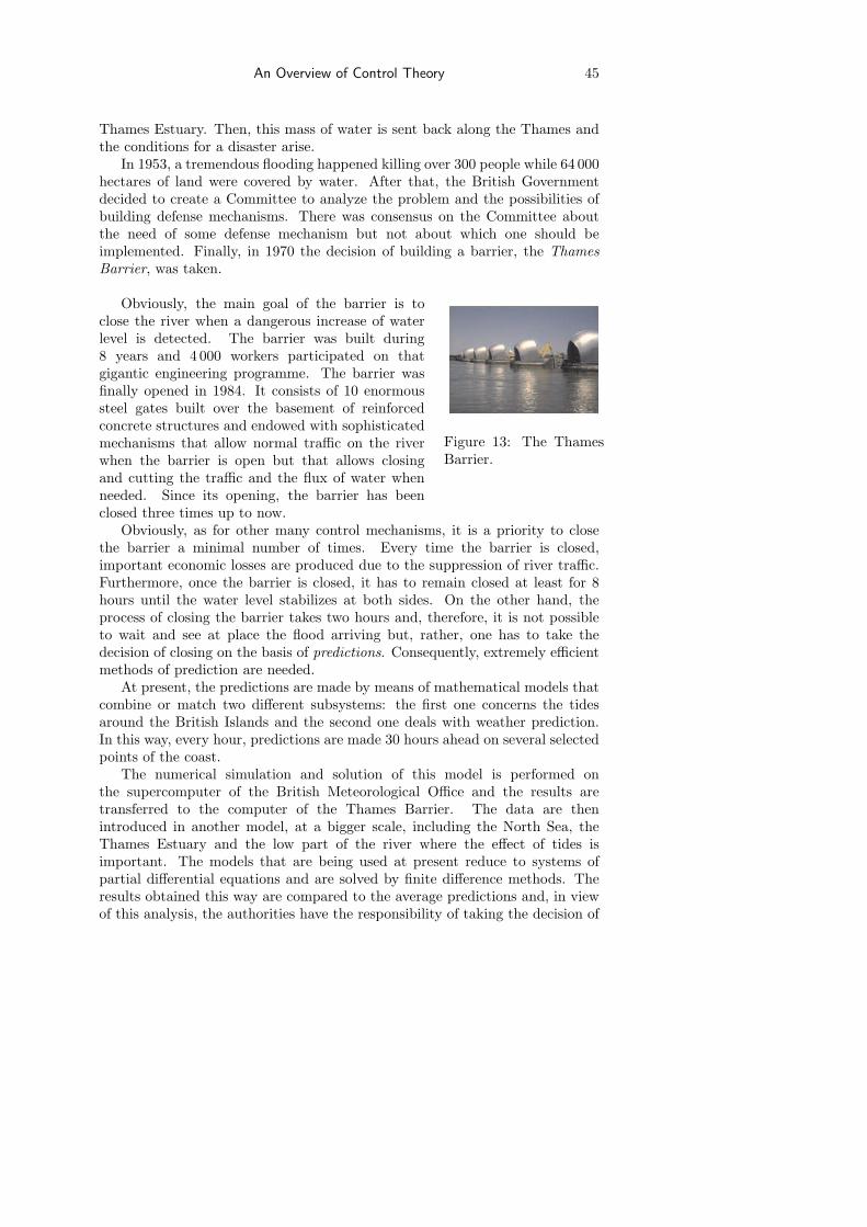
An Overview of Control Theory 45
Thames Estuary. Then, this mass of water is sent back along the Thames andthe conditions for a disaster arise.
In 1953, a tremendous flooding happened killing over 300 people while 64 000hectares of land were covered by water. After that, the British Governmentdecided to create a Committee to analyze the problem and the possibilities ofbuilding defense mechanisms. There was consensus on the Committee aboutthe need of some defense mechanism but not about which one should beimplemented. Finally, in 1970 the decision of building a barrier, the ThamesBarrier, was taken.
Figure 13: The ThamesBarrier.
Obviously, the main goal of the barrier is toclose the river when a dangerous increase of waterlevel is detected. The barrier was built during8 years and 4 000 workers participated on thatgigantic engineering programme. The barrier wasfinally opened in 1984. It consists of 10 enormoussteel gates built over the basement of reinforcedconcrete structures and endowed with sophisticatedmechanisms that allow normal traffic on the riverwhen the barrier is open but that allows closingand cutting the traffic and the flux of water whenneeded. Since its opening, the barrier has beenclosed three times up to now.
Obviously, as for other many control mechanisms, it is a priority to closethe barrier a minimal number of times. Every time the barrier is closed,important economic losses are produced due to the suppression of river traffic.Furthermore, once the barrier is closed, it has to remain closed at least for 8hours until the water level stabilizes at both sides. On the other hand, theprocess of closing the barrier takes two hours and, therefore, it is not possibleto wait and see at place the flood arriving but, rather, one has to take thedecision of closing on the basis of predictions. Consequently, extremely efficientmethods of prediction are needed.
At present, the predictions are made by means of mathematical models thatcombine or match two different subsystems: the first one concerns the tidesaround the British Islands and the second one deals with weather prediction.In this way, every hour, predictions are made 30 hours ahead on several selectedpoints of the coast.
The numerical simulation and solution of this model is performed onthe supercomputer of the British Meteorological Office and the results aretransferred to the computer of the Thames Barrier. The data are thenintroduced in another model, at a bigger scale, including the North Sea, theThames Estuary and the low part of the river where the effect of tides isimportant. The models that are being used at present reduce to systems ofpartial differential equations and are solved by finite difference methods. Theresults obtained this way are compared to the average predictions and, in viewof this analysis, the authorities have the responsibility of taking the decision of
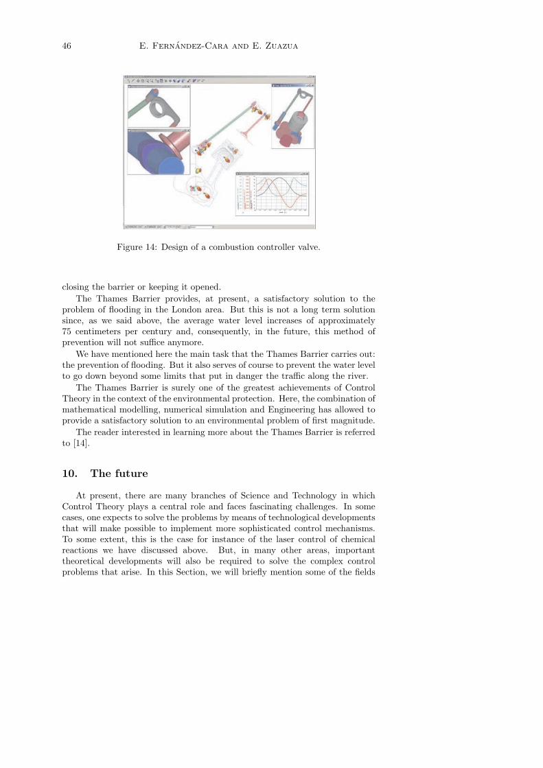
46 E. Fernandez-Cara and E. Zuazua
Figure 14: Design of a combustion controller valve.
closing the barrier or keeping it opened.The Thames Barrier provides, at present, a satisfactory solution to the
problem of flooding in the London area. But this is not a long term solutionsince, as we said above, the average water level increases of approximately75 centimeters per century and, consequently, in the future, this method ofprevention will not suffice anymore.
We have mentioned here the main task that the Thames Barrier carries out:the prevention of flooding. But it also serves of course to prevent the water levelto go down beyond some limits that put in danger the traffic along the river.
The Thames Barrier is surely one of the greatest achievements of ControlTheory in the context of the environmental protection. Here, the combination ofmathematical modelling, numerical simulation and Engineering has allowed toprovide a satisfactory solution to an environmental problem of first magnitude.
The reader interested in learning more about the Thames Barrier is referredto [14].
10. The future
At present, there are many branches of Science and Technology in whichControl Theory plays a central role and faces fascinating challenges. In somecases, one expects to solve the problems by means of technological developmentsthat will make possible to implement more sophisticated control mechanisms.To some extent, this is the case for instance of the laser control of chemicalreactions we have discussed above. But, in many other areas, importanttheoretical developments will also be required to solve the complex controlproblems that arise. In this Section, we will briefly mention some of the fields
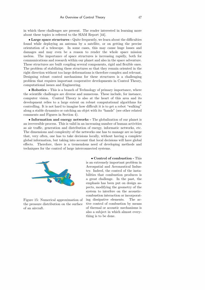
An Overview of Control Theory 47
in which these challenges are present. The reader interested in learning moreabout these topics is referred to the SIAM Report [44].
• Large space structures - Quite frequently, we learn about the difficultiesfound while deploying an antenna by a satellite, or on getting the preciseorientation of a telescope. In some cases, this may cause huge losses anddamages and may even be a reason to render the whole space missionuseless. The importance of space structures is increasing rapidly, both forcommunications and research within our planet and also in the space adventure.These structures are built coupling several components, rigid and flexible ones.The problem of stabilizing these structures so that they remain oriented in theright direction without too large deformations is therefore complex and relevant.Designing robust control mechanisms for these structures is a challengingproblem that requires important cooperative developments in Control Theory,computational issues and Engineering.
• Robotics - This is a branch of Technology of primary importance, wherethe scientific challenges are diverse and numerous. These include, for instance,computer vision. Control Theory is also at the heart of this area and itsdevelopment relies to a large extent on robust computational algorithms forcontrolling. It is not hard to imagine how difficult it is to get a robot “walking”along a stable dynamics or catching an objet with its “hands” (see other relatedcomments and Figures in Section 4).
• Information and energy networks - The globalization of our planet isan irreversible process. This is valid in an increasing number of human activitiesas air traffic, generation and distribution of energy, informatic networks, etc.The dimensions and complexity of the networks one has to manage are so largethat, very often, one has to take decisions locally, without having a completeglobal information, but taking into account that local decisions will have globaleffects. Therefore, there is a tremendous need of developing methods andtechniques for the control of large interconnected systems.
Figure 15: Numerical approximation ofthe pressure distribution on the surfaceof an aircraft.
• Control of combustion - Thisis an extremely important problem inAerospatial and Aeronautical Indus-try. Indeed, the control of the insta-bilities that combustion produces isa great challenge. In the past, theemphasis has been put on design as-pects, modifying the geometry of thesystem to interfere on the acoustic-combustion interaction or incorporat-ing dissipative elements. The ac-tive control of combustion by meansof thermal or acoustic mechanisms isalso a subject in which almost every-thing is to be done.
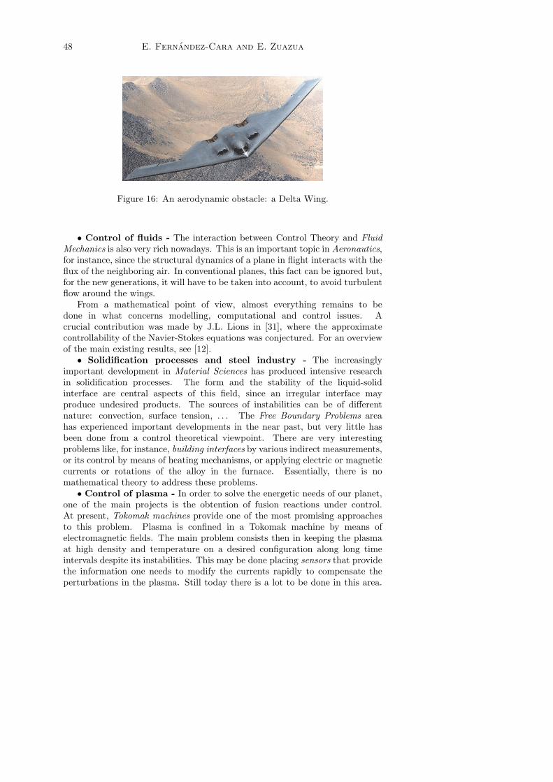
48 E. Fernandez-Cara and E. Zuazua
Figure 16: An aerodynamic obstacle: a Delta Wing.
• Control of fluids - The interaction between Control Theory and FluidMechanics is also very rich nowadays. This is an important topic in Aeronautics,for instance, since the structural dynamics of a plane in flight interacts with theflux of the neighboring air. In conventional planes, this fact can be ignored but,for the new generations, it will have to be taken into account, to avoid turbulentflow around the wings.
From a mathematical point of view, almost everything remains to bedone in what concerns modelling, computational and control issues. Acrucial contribution was made by J.L. Lions in [31], where the approximatecontrollability of the Navier-Stokes equations was conjectured. For an overviewof the main existing results, see [12].
• Solidification processes and steel industry - The increasinglyimportant development in Material Sciences has produced intensive researchin solidification processes. The form and the stability of the liquid-solidinterface are central aspects of this field, since an irregular interface mayproduce undesired products. The sources of instabilities can be of differentnature: convection, surface tension, . . . The Free Boundary Problems areahas experienced important developments in the near past, but very little hasbeen done from a control theoretical viewpoint. There are very interestingproblems like, for instance, building interfaces by various indirect measurements,or its control by means of heating mechanisms, or applying electric or magneticcurrents or rotations of the alloy in the furnace. Essentially, there is nomathematical theory to address these problems.
• Control of plasma - In order to solve the energetic needs of our planet,one of the main projects is the obtention of fusion reactions under control.At present, Tokomak machines provide one of the most promising approachesto this problem. Plasma is confined in a Tokomak machine by means ofelectromagnetic fields. The main problem consists then in keeping the plasmaat high density and temperature on a desired configuration along long timeintervals despite its instabilities. This may be done placing sensors that providethe information one needs to modify the currents rapidly to compensate theperturbations in the plasma. Still today there is a lot to be done in this area.
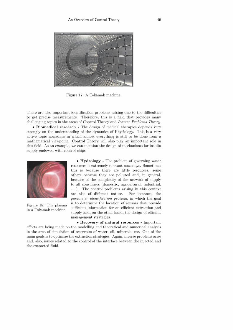
An Overview of Control Theory 49
Figure 17: A Tokamak machine.
There are also important identification problems arising due to the difficultiesto get precise measurements. Therefore, this is a field that provides manychallenging topics in the areas of Control Theory and Inverse Problems Theory.
• Biomedical research - The design of medical therapies depends verystrongly on the understanding of the dynamics of Physiology. This is a veryactive topic nowadays in which almost everything is still to be done from amathematical viewpoint. Control Theory will also play an important role inthis field. As an example, we can mention the design of mechanisms for insulinsupply endowed with control chips.
Figure 18: The plasmain a Tokamak machine.
• Hydrology - The problem of governing waterresources is extremely relevant nowadays. Sometimesthis is because there are little resources, someothers because they are polluted and, in general,because of the complexity of the network of supplyto all consumers (domestic, agricultural, industrial,. . . ). The control problems arising in this contextare also of different nature. For instance, theparameter identification problem, in which the goalis to determine the location of sensors that providesufficient information for an efficient extraction andsupply and, on the other hand, the design of efficientmanagement strategies.
• Recovery of natural resources - Importantefforts are being made on the modelling and theoretical and numerical analysisin the area of simulation of reservoirs of water, oil, minerals, etc. One of themain goals is to optimize the extraction strategies. Again, inverse problems ariseand, also, issues related to the control of the interface between the injected andthe extracted fluid.
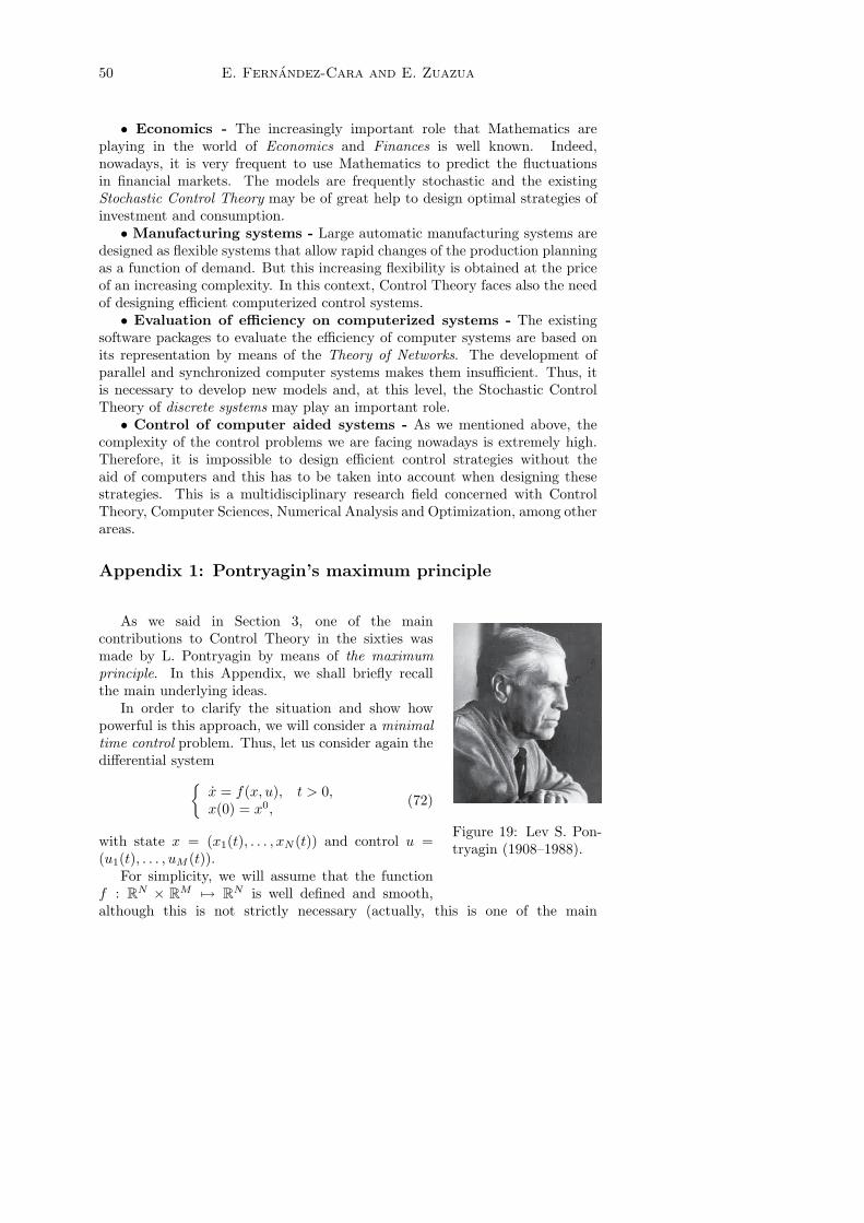
50 E. Fernandez-Cara and E. Zuazua
• Economics - The increasingly important role that Mathematics areplaying in the world of Economics and Finances is well known. Indeed,nowadays, it is very frequent to use Mathematics to predict the fluctuationsin financial markets. The models are frequently stochastic and the existingStochastic Control Theory may be of great help to design optimal strategies ofinvestment and consumption.
• Manufacturing systems - Large automatic manufacturing systems aredesigned as flexible systems that allow rapid changes of the production planningas a function of demand. But this increasing flexibility is obtained at the priceof an increasing complexity. In this context, Control Theory faces also the needof designing efficient computerized control systems.
• Evaluation of efficiency on computerized systems - The existingsoftware packages to evaluate the efficiency of computer systems are based onits representation by means of the Theory of Networks. The development ofparallel and synchronized computer systems makes them insufficient. Thus, itis necessary to develop new models and, at this level, the Stochastic ControlTheory of discrete systems may play an important role.
• Control of computer aided systems - As we mentioned above, thecomplexity of the control problems we are facing nowadays is extremely high.Therefore, it is impossible to design efficient control strategies without theaid of computers and this has to be taken into account when designing thesestrategies. This is a multidisciplinary research field concerned with ControlTheory, Computer Sciences, Numerical Analysis and Optimization, among otherareas.
Appendix 1: Pontryagin’s maximum principle
Figure 19: Lev S. Pon-tryagin (1908–1988).
As we said in Section 3, one of the maincontributions to Control Theory in the sixties wasmade by L. Pontryagin by means of the maximumprinciple. In this Appendix, we shall briefly recallthe main underlying ideas.
In order to clarify the situation and show howpowerful is this approach, we will consider a minimaltime control problem. Thus, let us consider again thedifferential system
x = f(x, u), t > 0,x(0) = x0,
(72)
with state x = (x1(t), . . . , xN (t)) and control u =(u1(t), . . . , uM (t)).
For simplicity, we will assume that the functionf : RN × RM 7→ RN is well defined and smooth,although this is not strictly necessary (actually, this is one of the main
An Overview of Control Theory 51
contributions of Pontryagin’s principle). We will also assume that a nonemptyclosed set G ⊂ RM is given and that the family of admissible controls is
Uad = u ∈ L2(0,+∞;RM ) : u(t) ∈ G a.e. . (73)
Let us introduce a manifold M of RN , with
M = x ∈ RN : µ(x) = 0 ,where µ : RN 7→ Rq is a regular map (q ≤ N), so that the matrix ∇µ(x) isof rank q at each point x ∈ M (thus, M is a smooth differential manifold ofdimension N − q). Recall that the tangent space to M at a point x ∈ M isgiven by:
TxM = v ∈ RN : ∇µ(x) · v = 0 .Let us fix the initial state x0 in RN \M. Then, to each control u = u(t) we
can associate a trajectory, defined by the solution of (72). Our minimal timecontrol problem consists in finding a control in the admissible set Uad drivingthe corresponding trajectory to the manifold M in a time as short as possible.
In other words, we intend to minimize the quantity T subject to the followingconstraints:
T > 0,
For some u ∈ Uad , the associated solution to (72) satisfies x(T ) ∈M.
Obviously, the difficulty of the problem increases when the dimension of Mdecreases.
The following result holds (Pontryagin’s maximum principle):
Theorem 6 Assume that T is the minimal time and u, defined for t ∈ [0, T ], isan optimal control for this problem. Let x be the corresponding trajectory. Thenthere exists p = p(t) such that the following identities hold almost everywherein [0, T ]:
˙x = f(x, u), − ˙p =(
∂f
∂x(x, u)
)t
· p (74)
andH(x(t), p(t), u) = max
v∈GH(x(t), p(t), v), (75)
whereH(x, p, v) = 〈f(x, v), p〉 ∀(x, p, v) ∈ RN × RN ×G. (76)
Furthermore, the quantity
H∗(x, p) = maxv∈G
H(x, p, v) (77)
is constant and nonnegative (maximum condition) and we have
x(T ) = x0, x(T ) ∈M (78)
52 E. Fernandez-Cara and E. Zuazua
andp(T ) ⊥ Tx(T )M (79)
(transversality condition).
The function H is referred to as the Hamiltonian of (72) and the solutions(x, p, u) of the equations (74)–(79) are called extremal points. Of course, p isthe extremal adjoint state.
Very frequently in practice, in order to compute the minimal time T andthe optimal control u, system (74)–(79) is used as follows. First, assuming thatx and p are known, we determine u(t) for each t from (75). Then, with ubeing determined in terms of x and p, we solve (74) with the initial and finalconditions (78) and (79).
Observe that this is a well posed boundary-value problem for the couple(x, p) in the time interval (0, T ).
From (74), the initial and final conditions and (75), provide the control interms of the state. Consequently, the maximum principle can be viewed as afeedback law for determining a good control u.
In order to clarify the statement in Theorem 6, we will now present aheuristic proof.
We introduce the Hilbert space X × U , where U = L2(0, +∞;RM ) andX is the space of functions x = x(t) satisfying x ∈ L2(0,+∞;RN ) andx ∈ L2(0,+∞;RN )5.
Let us consider the functional
F (T, x, u) = T ∀(T, x, u) ∈ R×X × U .
Then, the problem under consideration is
To minimize F (T, x, u), (80)
subject to the inequality constraint
T ≥ 0, (81)
the pointwise control constraints
u(t) ∈ G a.e. in (0, T ) (82)
(that is to say u ∈ Uad) and the equality constraints
x− f(x, u) = 0 a.e. in (0, T ), (83)
x(0)− x0 = 0 (84)
andµ(x(T )) = 0. (85)
5This is the Sobolev space H1(0, +∞;RN ). More details can be found, for instance, in [3].
An Overview of Control Theory 53
Let us assume that (T , x, u) is a solution to this constrained extremalproblem. One can then prove the existence of Lagrange multipliers (p, z, w) ∈X × RN × RN such that (T , x, u) is, together with (p, z, w), a saddle point ofthe Lagrangian
L(T, x, u; p, z, w) = T +∫ T
0
〈p, x− f(x, u)〉 dt + 〈z, x(0)− x0〉+ 〈w, µ(x(T ))〉
in R+ ×X × Uad ×X × RN × RN .In other words, we have
L(T , x, u; p, z, w) ≤ L(T , x, u; p, z, w) ≤ L(T, x, u; p, z, w)∀(T, x, u) ∈ R+ ×X × Uad , ∀(p, z, w) ∈ X × RN × RN .
(86)
The first inequalities in (86) indicate that the equality constraints (83)−(85)are satisfied for T , x and u. Let us now see what is implied by the secondinequalities in (86).
First, taking T = T and x = x and choosing u arbitrarily in Uad , we findthat ∫ T
0
〈p, f(x, u)〉 dt ≤∫ T
0
〈p, f(x, u)〉 dt ∀u ∈ Uad .
It is not difficult to see that this is equivalent to (75), in view of the definitionof Uad .
Secondly, taking T = T and u = u, we see that
∫ T
0
〈p, x− f(x, u)〉 dt + 〈z, x(0)− x0〉+ 〈w, µ(x(T ))〉 ≥ 0 ∀x ∈ X. (87)
From (87) written for x = x ± εy, taking into account that (83) − (85) aresatisfied for T , x and u, after passing to the limit as ε → 0, we easily find that
∫ T
0
〈p, y− ∂f
∂x(x, u) ·y〉 dt+ 〈z, y(0)〉+ 〈w,∇µ(x(T )) ·y(T )〉 = 0 ∀y ∈ X. (88)
Taking y ∈ X such that y(0) = y(T ) = 0, we can deduce at once thedifferential system satisfied by p in (0, T ). Indeed, after integration by parts,we have from (88) that
∫ T
0
〈− ˙p−(
∂f
∂x(x, u)
)t
· p, y〉 dt = 0
for all such y. This leads to the second differential system in (74).Finally, let us fix λ in RN an let us take in (88) a function y ∈ X such that
y(0) = 0 and y(T ) = λ. Integrating again by parts, in view of (74), we find that
〈p(T ), λ〉+ 〈w,∇µ(x(T )) · λ〉 = 0
54 E. Fernandez-Cara and E. Zuazua
and, since λ is arbitrary, this implies
p(T ) = −(∇µ(x(T ))
)t
w.
This yields the transversality condition (79).We have presented here the maximum principle for a minimal time control
problem, but there are many variants and generalizations.For instance, let the final time T > 0 and a non-empty closed convex set
S ⊂ RN be fixed and let Uad be now the family of controls u ∈ L2(0, T ;RM )with values in the closed set G ⊂ RM such that the associated states x = x(t)satisfy
x(0) = x0, x(T ) ∈ S. (89)
Let f0 : RN × RM 7→ R be a smooth bounded function and let us put
F (u) =∫ T
0
f0(x(t), u(t)) dt ∀u ∈ Uad , (90)
where x is the state associated to u through (72). In this case, the HamiltonianH is given by
H(x, p, u) = 〈f(x, u), p〉+ f0(x, u) ∀(x, p, u) ∈ RN × RN ×G. (91)
Then, if u minimizes F over Uad and x is the associated state, the maximumprinciple guarantees the existence of a function p such that the following systemholds:
˙x = f(x, u), − ˙p =(
∂f
∂x(x, u)
)t
· p +∂f0
∂x(x, u) a.e. in (0,T), (92)
H(x(t), p(t), u) = maxv∈G
H(x(t), p(t), v), (93)
x(0) = x0, x(T ) ∈ S (94)
and〈p(T ), y − x(T )〉 ≥ 0 ∀y ∈ S. (95)
For general nonlinear systems, the optimality conditions that the Pontryaginmaximum principle provides may be difficult to analyze. In fact, in many cases,these conditions do not yield a complete information of the optimal trajectories.Very often, this requires appropriate geometrical tools, as the Lie bracketsmentioned in Section 4. The interested reader is referred to H. Sussmann [48]for a more careful discussion of these issues.
In this context, the work by J.A. Reeds and L.A. Shepp [39] is worthmentioning. This paper is devoted to analyze a dynamical system for avehicle, similar to the one considered at the end of Section 4, but allowingboth backwards and forwards motion. As an example of the complexity of thedynamics of this system, it is interesting to point out that an optimal trajectoryconsists of, at most, five pieces. Each piece is either a segment or an arc of
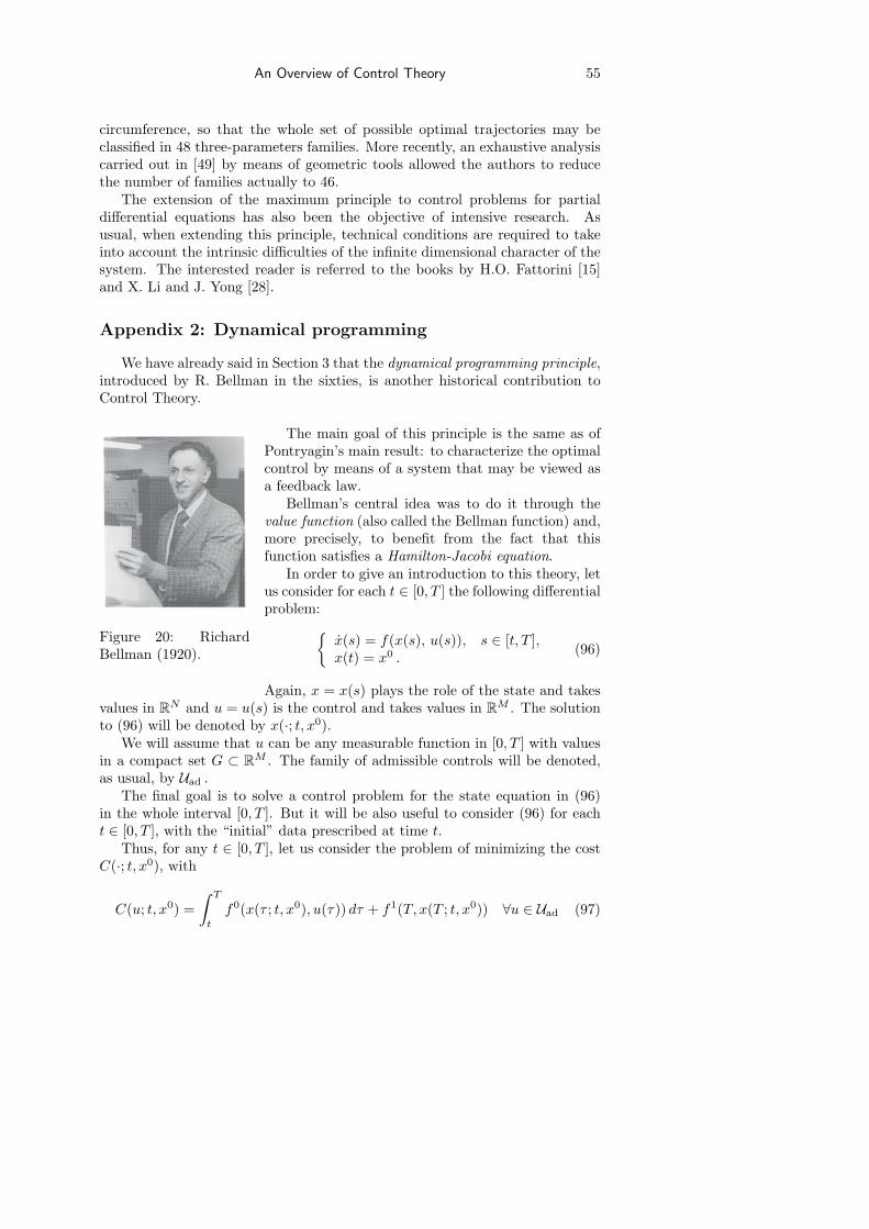
An Overview of Control Theory 55
circumference, so that the whole set of possible optimal trajectories may beclassified in 48 three-parameters families. More recently, an exhaustive analysiscarried out in [49] by means of geometric tools allowed the authors to reducethe number of families actually to 46.
The extension of the maximum principle to control problems for partialdifferential equations has also been the objective of intensive research. Asusual, when extending this principle, technical conditions are required to takeinto account the intrinsic difficulties of the infinite dimensional character of thesystem. The interested reader is referred to the books by H.O. Fattorini [15]and X. Li and J. Yong [28].
Appendix 2: Dynamical programming
We have already said in Section 3 that the dynamical programming principle,introduced by R. Bellman in the sixties, is another historical contribution toControl Theory.
Figure 20: RichardBellman (1920).
The main goal of this principle is the same as ofPontryagin’s main result: to characterize the optimalcontrol by means of a system that may be viewed asa feedback law.
Bellman’s central idea was to do it through thevalue function (also called the Bellman function) and,more precisely, to benefit from the fact that thisfunction satisfies a Hamilton-Jacobi equation.
In order to give an introduction to this theory, letus consider for each t ∈ [0, T ] the following differentialproblem:
x(s) = f(x(s), u(s)), s ∈ [t, T ],x(t) = x0 .
(96)
Again, x = x(s) plays the role of the state and takesvalues in RN and u = u(s) is the control and takes values in RM . The solutionto (96) will be denoted by x(·; t, x0).
We will assume that u can be any measurable function in [0, T ] with valuesin a compact set G ⊂ RM . The family of admissible controls will be denoted,as usual, by Uad .
The final goal is to solve a control problem for the state equation in (96)in the whole interval [0, T ]. But it will be also useful to consider (96) for eacht ∈ [0, T ], with the “initial” data prescribed at time t.
Thus, for any t ∈ [0, T ], let us consider the problem of minimizing the costC(·; t, x0), with
C(u; t, x0) =∫ T
t
f0(x(τ ; t, x0), u(τ)) dτ + f1(T, x(T ; t, x0)) ∀u ∈ Uad (97)
56 E. Fernandez-Cara and E. Zuazua
(the final goal is to minimize C(·; 0, x0) in the set of admissible controls Uad).To simplify our exposition, we will assume that the functions f , f0 and f1 areregular and bounded with bounded derivatives.
The main idea in dynamical programming is to introduce and analyze the socalled value function V = V (x0, t), where
V (x0, t) = infu∈Uad
C(u; t, x0) ∀x0 ∈ RN , ∀t ∈ [0, T ]. (98)
This function provides the minimal cost obtained when the system startsfrom x0 at time t and evolves for s ∈ [t, T ]. The main property of V is that itsatisfies a Hamilton-Jacobi equation. This fact can be used to characterize andeven compute the optimal control.
Before writing the Hamilton-Jacobi equation satisfied by V , it is convenientto state the following fundamental result:
Theorem 7 The value function V = V (x0, t) satisfies the Bellman optimalityprinciple, or dynamical programming principle. According to it, for any x0 ∈RN and any t ∈ [0, T ], the following identity is satisfied:
V (x0, t) = infu∈Uad
[V (x(s; t, x0), s) +
∫ s
t
f0(x(τ ; t, x0), u(τ)) dτ
]∀s ∈ [t, T ].
(99)
In other words, the minimal cost that is produced starting from x0 at timet coincides with the minimal cost generated starting from x(s; t, x0) at time splus the “energy” lost during the time interval [t, s]. The underlying idea is thata control, to be optimal in the whole time interval [0, T ], has also to be optimalin every interval of the form [t, T ].
A consequence of (99) is the following:
Theorem 8 The value function V = V (x, t) is globally Lipschitz-continuous.Furthermore, it is the unique viscosity solution of the following Cauchy problemfor the Hamilton-Jacobi-Bellman equation
Vt + inf
v∈G
〈f(x, v),∇V 〉+ f0(x, v)
= 0, (x, t) ∈ RN × (0, T ),
V (x, T ) = f1(T, x), x ∈ RN .(100)
The equation in (100) is, indeed, a Hamilton-Jacobi equation, i.e. anequation of the form
Vt + H(x,∇V ) = 0,
with Hamiltonian
H(x, p) = infv∈G
〈f(x, v), p〉+ f0(x, v)
(101)
(recall (91)).The notion of viscosity solution of a Hamilton-Jacobi equation was
introduced to compensate the absence of existence and uniqueness of classical
An Overview of Control Theory 57
solution, two phenomena that can be easily observed using the method ofcharacteristics. Let us briefly recall it.
Assume that H = H(x, p) is a continuous function (defined for (x, p) ∈RN ×RN ) and g = g(x) is a continuous bounded function in RN . Consider thefollowing initial-value problem:
yt + H(x,∇y) = 0, (x, t) ∈ RN × (0,∞),y(x, 0) = g(x), x ∈ RN .
(102)
Let y = y(x, t) be bounded and continuous. It will be said that y is a viscositysolution of (102) if the following holds:
• For each v ∈ C∞(RN × (0,∞)), one has
If y − v has a local maximum at (x0, t0) ∈ RN × (0,∞), thenvt(x0, t0) + H(x0,∇v(x0, t0)) ≤ 0
and
If y − v has a local minimum at (x0, t0) ∈ RN × (0,∞), thenvt(x0, t0) + H(x0,∇v(x0, t0)) ≥ 0.
• y(x, 0) = g(x) for all x ∈ RN .
This definition is justified by the following fact. Assume that y is a classicalsolution to (102). It is then easy to see that, whenever v ∈ C∞(RN × (0,∞))and vt(x0, t0)+H(x0,∇v(x0, t0)) > 0 (resp. < 0), the function y−v cannot havea local maximum (resp. a local minimum) at (x0, t0). Consequently, a classicalsolution is a viscosity solution and the previous definition makes sense.
On the other hand, it can be checked that the solutions to (102) obtainedby the vanishing viscosity method satisfy these conditions and, therefore, areviscosity solutions. The vanishing viscosity method consists in solving, for eachε > 0, the parabolic problem
yt + H(x,∇y) = ε∆y, (x, t) ∈ RN × (0,∞),y(x, 0) = g(x), x ∈ RN (103)
and, then, passing to the limit as ε → 0+.A very interesting feature of viscosity solutions is that the two properties
entering in its definition suffice to prove uniqueness. The proof of this uniquenessresult is inspired on the pioneering work by N. Kruzhkov [22] on entropysolutions for hyperbolic equations. The most relevant contributions to thissubject are due to M. Crandall and P.L. Lions and L.C. Evans, see [6], [10].
But let us return to the dynamical programming principle (the fact that thevalue function V satisfies (99)) and let us see how can it be used.
One may proceed as follows. First, we solve (100) and obtain in this waythe value function V . Then, we try to compute u(t) at each time t using theidentities
f(x(t), u(t)) · ∇V (x(t), t) + f0(x(t), u(t)) = H(x(t),∇V (x(t), t)), (104)
58 E. Fernandez-Cara and E. Zuazua
i.e. we look for the values u(t) such that the minimum of the Hamiltonian in(101) is achieved. In this way, we can expect to obtain a function u = u(t)which is the optimal control.
Recall that, for each u, the state x is obtained as the solution of ˙x(s) = f (x(s), u(s)) , s ∈ [0, T ],
x(0) = x0 .(105)
Therefore, x is determined by u and (104) is an equation in which u(t) is in factthe sole unknown.
In this way, one gets indeed an optimal control u in feedback form thatprovides an optimal trajectory x (however, at the points where V is not smooth,important difficulties arise; for instance, see [16]).
If we compare the results obtained by means of the maximum principle andthe dynamical programming principle, we see that, in both approaches, themain conclusions are the same. It could not be otherwise, since the objectivewas to characterize optimal controls and trajectories.
However, it is important to underline that the points of view are completelydifferent. While Pontryagin’s principle extends the notion of Lagrangemultiplier, Bellman’s principle provides a dynamical viewpoint in which thevalue function and its time evolution play a crucial role.
The reader interested in a simple but relatively complete introduction toHamilton-Jacobi equations and dynamical programming can consult the bookby L.C. Evans [11]. For a more complete analysis of these questions see forinstance W. Fleming and M. Soner [16] and P.-L. Lions [32]. For an extensionof these methods to partial differential equations, the reader is referred to thebook by X. Li and J. Yong [28].
References
[1] J. Achache and A. Bensoussan, Assimilation, simulation et prevision,MATAPLI, 60 (1999), 25–34.
[2] S. Bennet, A History of Control Engineering 1800–1930, IEE ControlEngineering Series 8, Peter Peregrinus Ltd., London 1979.
[3] H. Brezis, Analyse Fonctionnelle, Masson, Paris 1996.
[4] P. Brumer and M. Shapiro, Laser control of chemical reactions, ScientificAmerican, 1995, p. 34–39.
[5] J. Cea, Optimisation: Theorie et Algorithmes, Dunod, Gauthiers-Villars,Paris 1971.
[6] M. Crandall and P.L. Lions, Viscosity solutions of Hamilton-Jacobiequations, Trans. Amer. Math. Soc. 277 (1983), no. 1, 1–42.
[7] R. Courant and D. Hilbert, Methods of Mathematical Physics, Vol. II,Interscience Publishers, New York 1962.
An Overview of Control Theory 59
[8] R.C. Dorf, Sistemas Modernos de Control, Addison-Wesley Iberoameri-cana, Madrid 1989.
[9] I. Ekeland and R. Temam, Analyse Convexe et Problemes Variationnels,Dunnod, Paris 1974.
[10] L.C. Evans, On solving certain nonlinear partial differential equations byaccretive operator methods, Israel J. Math. 36 (1980), no. 3-4, 225–247.
[11] L.C. Evans, Partial Differential Equations, American MathematicalSociety, Graduate Texts in Mathematics, 19, 1998.
[12] E. Fernandez-Cara, On the approximate and null controllability of theNavier-Stokes equations, SIAM Rev. 41 (1999), no. 2, p. 269–277.
[13] E. Fernandez-Cara and S. Guerrero Global Carleman inequalities forparabolic systems and applications to null controllability, to appear.
[14] D.G. Farmer and M.J. Rycroft, Computer Modelling in the EnvironmentalSciences, Clarendon Press, Oxford 1991.
[15] H.O. Fattorini, Infinite Dimensional Optimization and Control Theory,Encyclopedia of Mathematics and its Applications 62, CambridgeUniversity Press, 1999.
[16] W. Fleming and M. Soner, Controlled Markov Processes and ViscositySolutions, Springer-Verlag, New York 1993.
[17] H.R. Hall, Governors and Governing Mechanisms, The TechnicalPublishing Co., 2nd ed., Manchester 1907.
[18] J.A. Infante and E. Zuazua, Boundary observability for the space semi-discretizations of the 1− d wave equation, M2AN , 33 (2) (1999), 407–438.
[19] R. Glowinski, Numerical Methods for Nonlinear Variational Problems (2ndEdition), Springer-Verlag, New York 1984.
[20] O. Kavian, Introduction a la Theorie des Points Critiques, Mathematiques& Applications, 13, Paris 1993.
[21] V. Komornik, Exact controllability and stabilization. The multipliermethod, Masson, John Wiley & Sons, Chichester 1994.
[22] N.S. Kruzhkov, First-order quasilinear equations in several independentvariables, Mat. USSR-Sb., 10 (1970), 217–243.
[23] B. Larrouturou and P.-L. Lions, Methodes mathematiques pour les sciencesde l’ingenieur: Optimisation et analyse numerique, Publications de l’EcolePolytechnique de Paris, 1996.
[24] P. Le Tallec, Domain decomposition methods in computational mechanics,Comp. Mechanics Advances, 1 (1994), 121–220.
60 E. Fernandez-Cara and E. Zuazua
[25] E.B. Lee and L. Markus, Foundations of Optimal Control Theory, TheSIAM Series in Applied Mathematics, John Wiley & Sons, New York 1967.
[26] W.S. Levine, Control System and Applications, CRC Press, 2000.
[27] I. Lasiecka and R. Triggiani, Control Theory for Partial DifferentialEquations: Continuous and Approximation Theories, Vol. I and II.Encyclopedia of Mathematics and its Applications, 74–75, CambridgeUniversity Press, Cambridge 2000.
[28] X. Li and J. Yong, Optimal Control Theory for Infinite DimensionalSystems, Birkhauser, Boston 1995.
[29] J.L. Lions, Exact controllability, stabilizability and perturbations fordistributed systems, SIAM Review, 30 (1988), 1–68.
[30] J.L. Lions, Controlabilite Exacte, Stabilisation et Perturbations deSystemes Distribues, Tomes 1 & 2. Masson, RMA 8 & 9, Paris 1988.
[31] J.L. Lions, Remarques sur la controlabilite approchee, in “Spanish-FrenchConference on Distributed-Systems Control”, Univ. Malaga, 1990, p. 77–87.
[32] P.-L. Lions, Generalized Solutions of Hamilton-Jacobi Equations. ResearchNotes in Mathematics, 69, Pitman, New York 1982.
[33] O. Mayr, The origins of Feedback Control, MIT Press, Cambridge, MA,1970.
[34] J. Mohammadi and O. Pironneau, Applied Shape Optimization for Fluids,The Clarendon Press, Oxford University Press, New York 2001.
[35] P. Moin and Th. Bewley, Feedback control of turbulence, in “MechanicsUSA 1994”, A.S. Kobayashi ed., Appl. Mech. Rev., 47 (6) (1994), S3–S13.
[36] K. Ogata, Ingenierıa de Control Moderna, Prentice Hall Hispanoamericana,Madrid 1998.
[37] O. Pironneau, Optimal Shape Design for Elliptic Systems, Springer-Verlag,New York 1984.
[38] A. Prohl, Projection and Quasi-Compressibility Methods for Solvingthe Incompressible Navier-Stokes Equations, Advances in NumericalMathematics, B.G. Teubner, Stuttgart 1997.
[39] J.A. Reeds and L.A. Shepp, Optimal paths for a car that goes both forwardsand backwards, Pacific J. Math., 145 (1990), 367–393.
[40] S.S. Rao, Optimization. Theory and Applications, 2nd edition, John Wiley& Sons, New York 1984.
An Overview of Control Theory 61
[41] R.T. Rockafellar, Convex Analysis, Princeton University Press, Princeton1970.
[42] D.L. Russell, Controllability and stabilizability theory for linear partialdifferential equations. Recent progress and open questions, SIAM Review20 (1978), 639–739.
[43] M. Salomone, Los humanoides ya estan aquı, El Paıs Semanal, 12338, June18th, 2000.
[44] S.I.A.M., Future Directions in Control Theory, Report of the Panelof Future Directions in Control Theory, SIAM Report on Issues inMathematical Sciences, Philadelphia, 1988.
[45] D.R. Smith, Variational Methods in Optimization, Prentice-Hall,Englewood Cliffs, N.J., 1974.
[46] E.D. Sontag, Mathematical Control Theory. Deterministic FiniteDimensional Systems (2nd Edition), Texts in Applied Mathematics, 6,Springer-Verlag, New York 1998.
[47] G. Strang, Introduction to Applied Mathematics, Wellesley-CambridgePress, Massachusetts, 1986.
[48] H.J. Sussmann, Resultats recents sur les courbes optimales, JourneeAnnuelle SMF, June 2000, (http://www.math.rutgers.edu/~sussmann).
[49] H.J. Sussmann and G. Tang, Shortest paths for the Reeds-Shepp car,in “Rutgers Center for Systems and Control (SYCON)”, Report 91-10,September 1991.
[50] R.H. Thurston, A History of the Growth of the Steam-Engine(Web document), Stevens Institute of Technology, Hoboken, N.J.http://www.history.rochester.edu/steam/thurston/1878/.
[51] R. Varga, Matrix Iterative Analysis, 2nd edition, Springer-Verlag, Berlin,2000.
[52] R.M. Young, An Introduction to Nonharmonic Fourier Series, AcademicPress, New York 1980.
[53] O.C. Zienkiewicz, Achievements and some unsolved problems of the finiteelement method, Int. J. Numer. Meth. Eng. 47 (2000), 9–28.
[54] E. Zuazua, Some Problems and Results on the controllability of PartialDifferential Equations, in “Proceedings of the Second European Congress ofMathematics”, Budapest, July 1996. Progress in Mathematics, 169, 1998,Birkhauser Verlag Basel/Switzerland, pp. 276–311.
62 E. Fernandez-Cara and E. Zuazua
[55] E. Zuazua, Controllability of Partial Differential Equations and its Semi-Discrete Approximation, Discrete and Continuous Dynamical Systems, 8(2) (2002), 469-513.
[56] E. Zuazua, Propagation, Observation, Control and Numerical Approxima-tion of Waves, Bol. Soc. Esp. Mat. Apl. No. 25 (2003), 55–126.
[57] E. Zuazua, Remarks on the controllability of the Schrodinger equation,in “Quantum Control: Mathematical and Numerical Challenges”,A. Bandrauk, M.C. Delfour and C. Le Bris eds., CRM Proc. Lecture NotesSeries 33, AMS Publications, Providence, R.I. 2003, pp. 181–199.