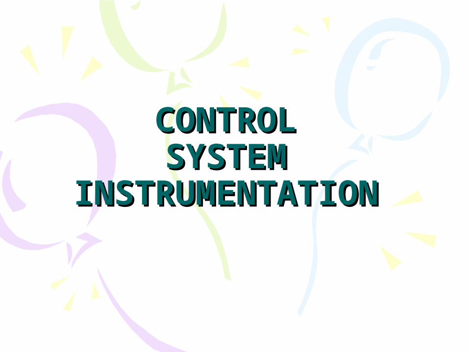
CONTROLCONTROLSYSTEM SYSTEM

INSTRUMENTATIONINSTRUMENTATION

Control System Instrumentation

Figure 9.3 A typical process transducer.

Transducers and Transmitters• Figure 9.3 illustrates the general configuration of a

measurement transducer; it typically consists of a sensing element combined with a driving element (transmitter).

• Transducers for process measurements convert the magnitude of a process variable (e.g., flow rate, pressure, temperature, level, or concentration) into a signal that can be sent directly to the controller.

• The sensing element is required to convert the measured quantity, that is, the process variable, into some quantity more appropriate for mechanical or electrical processing within the transducer.

Standard Instrumentation Signal Levels

• Before 1960, instrumentation in the process industries utilized pneumatic (air pressure) signals to transmit measurement and control information almost exclusively.

• These devices make use of mechanical force-balance elements to generate signals in the range of 3 to 15 psig, an industry standard.

• Since about 1960, electronic instrumentation has come into widespread use.

Sensors

The book briefly discusses commonly used sensors for the most important process variables. (See text.)

Transmitters• A transmitter usually converts the sensor output to a signal level

appropriate for input to a controller, such as 4 to 20 mA.

• Transmitters are generally designed to be direct acting.

• In addition, most commercial transmitters have an adjustable input range (or span).

• For example, a temperature transmitter might be adjusted so that the input range of a platinum resistance element (the sensor) is 50 to 150 °C.

Ch

apte

r 9

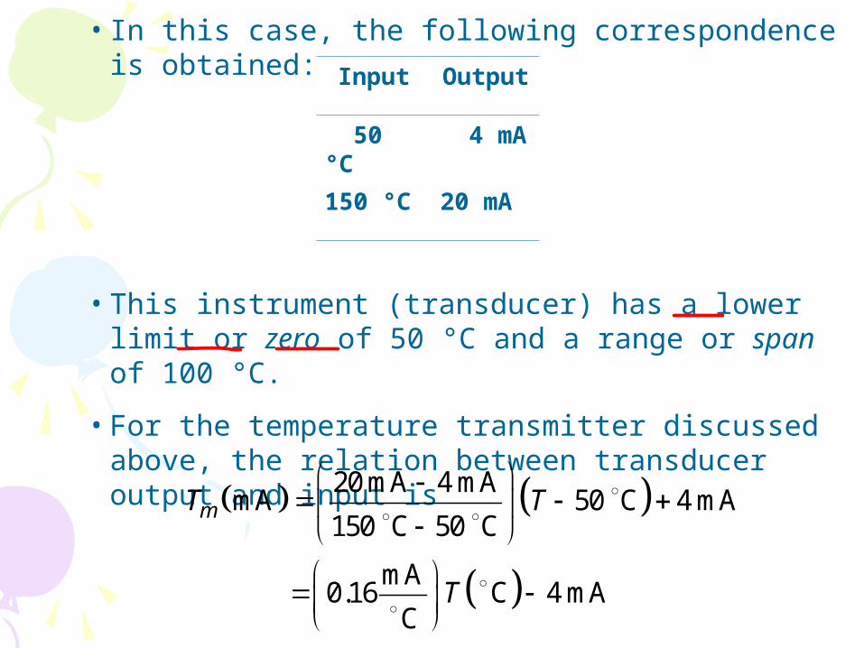
• In this case, the following correspondence is obtained:

Input Output

50 °C 4 mA

150 °C 20 mA

• This instrument (transducer) has a lower limit or zero of 50 °C and a range or span of 100 °C.

• For the temperature transmitter discussed above, the relation between transducer output and input is

20 mA 4 mAmA 50 C 4 mA

150 C 50 C

mA0.16 C 4 mA

C

mT T

T

The gain of the measurement element Km is 0.16 mA/°C. For any linear instrument:

range of instrument output(9-1)

range of instrument inputmK

Final Control Elements

• Every process control loop contains a final control element (actuator), the device that enables a process variable to be manipulated.

• For most chemical and petroleum processes, the final control elements (usually control valves) adjust the flow rates of materials, and indirectly, the rates of energy transfer to and from the process.

Figure 9.4 A linear instrument calibration showing its zero and span.

Control Valves

• There are many different ways to manipulate the flows of material and energy into and out of a process; for example, the speed of a pump drive, screw conveyer, or blower can be adjusted.

• However, a simple and widely used method of accomplishing this result with fluids is to use a control valve, also called an automatic control valve.

• The control valve components include the valve body, trim, seat, and actuator.

Air-to-Open vs. Air-to-Close Control Valves

• Normally, the choice of A-O or A-C valve is based on safety considerations.

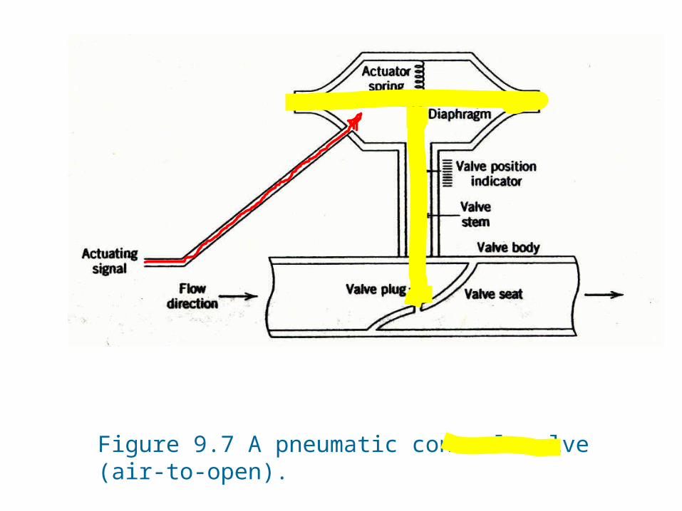
Figure 9.7 A pneumatic control valve (air-to-open).

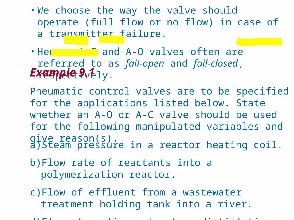
• We choose the way the valve should operate (full flow or no flow) in case of a transmitter failure.

• Hence, A-C and A-O valves often are referred to as fail-open and fail-closed, respectively.

Example 9.1

Pneumatic control valves are to be specified for the applications listed below. State whether an A-O or A-C valve should be used for the following manipulated variables and give reason(s).

a) Steam pressure in a reactor heating coil.

b) Flow rate of reactants into a polymerization reactor.

c) Flow of effluent from a wastewater treatment holding tank into a river.

d) Flow of cooling water to a distillation condenser.

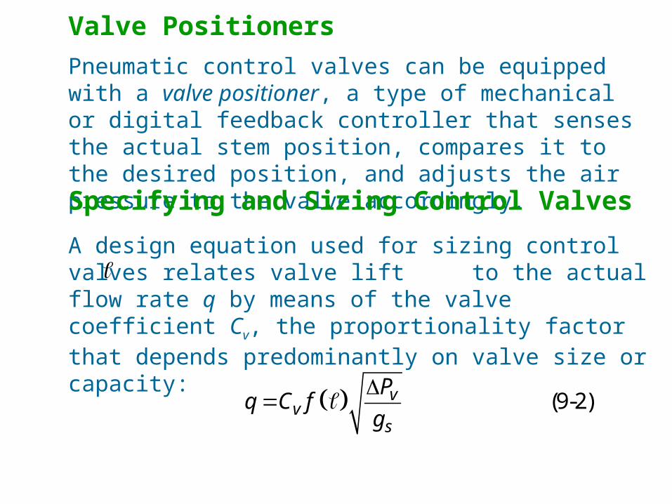
Valve Positioners

Pneumatic control valves can be equipped with a valve positioner, a type of mechanical or digital feedback controller that senses the actual stem position, compares it to the desired position, and adjusts the air pressure to the valve accordingly.

Specifying and Sizing Control Valves

A design equation used for sizing control valves relates valve lift to the actual flow rate q by means of the valve coefficient Cv, the proportionality factor that depends predominantly on valve size or capacity:

(9-2)vv

s

Pq C f

g

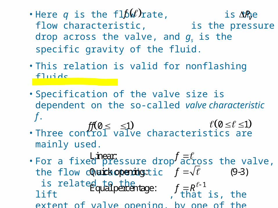
• Here q is the flow rate, is the flow characteristic, is the pressure drop across the valve, and gs is the specific gravity of the fluid.

• This relation is valid for nonflashing fluids.

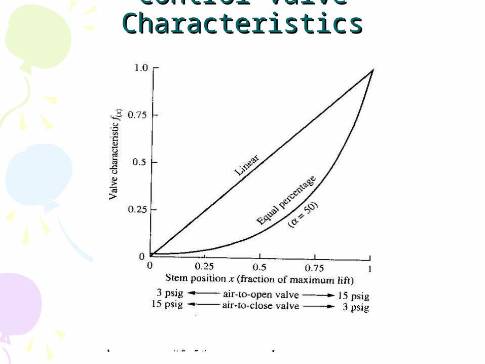
• Specification of the valve size is dependent on the so-called valve characteristic f.

• Three control valve characteristics are mainly used.

• For a fixed pressure drop across the valve, the flow characteristic is related to the lift , that is, the extent of valve opening, by one of the following relations:

f vP

0 1f f 0 1

1

Linear:

Quick opening: (9-3)

Equal percentage:

f

f

f R

Figure 9.8 Control valve characteristics.

Figure 9.16 Schematic diagram of a thermowell/thermocouple.

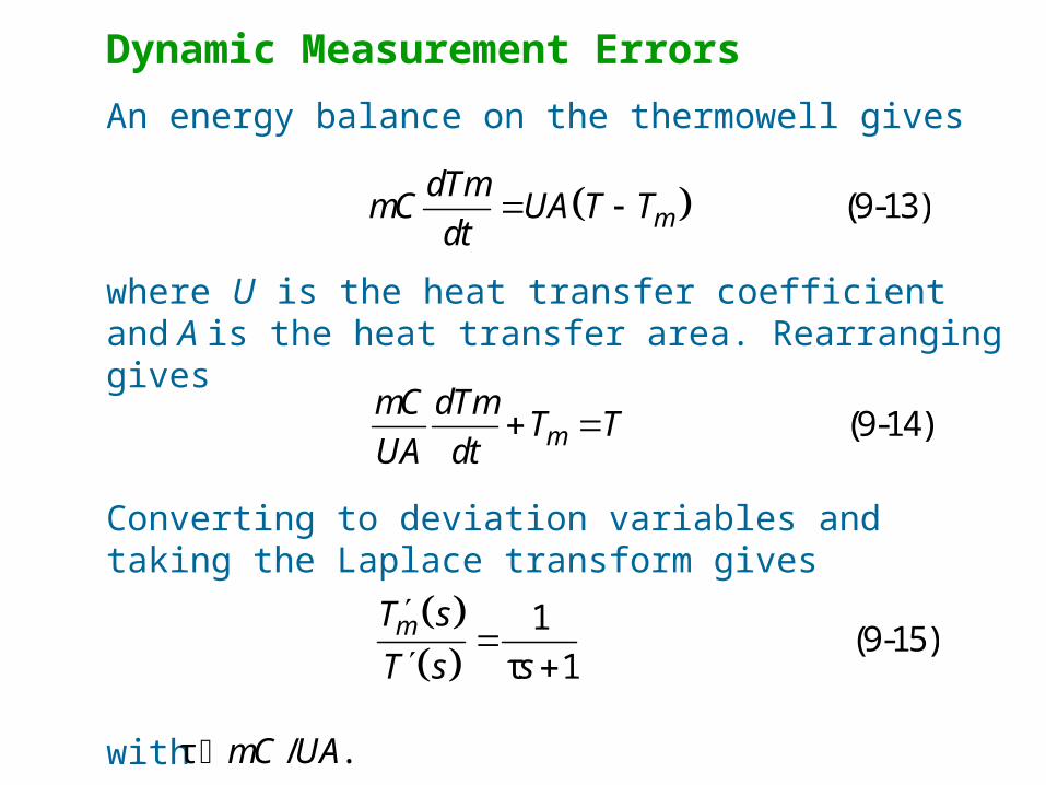
Dynamic Measurement Errors

An energy balance on the thermowell gives

(9-13)mdTm

mC UA T Tdt

where U is the heat transfer coefficient and A is the heat transfer area. Rearranging gives

(9-14)mmC dTm

T TUA dt

Converting to deviation variables and taking the Laplace transform gives

1(9-15)

τ 1mT s

T s s

with τ / .mC UA

Figure 9.13 Analysis of types of error for a flow instrument whose range is 0 to 4 flow units.

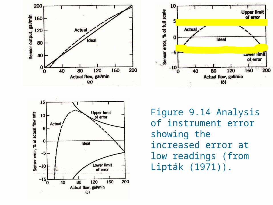
Figure 9.14 Analysis of instrument error showing the increased error at low readings (from Lipták (1971)).

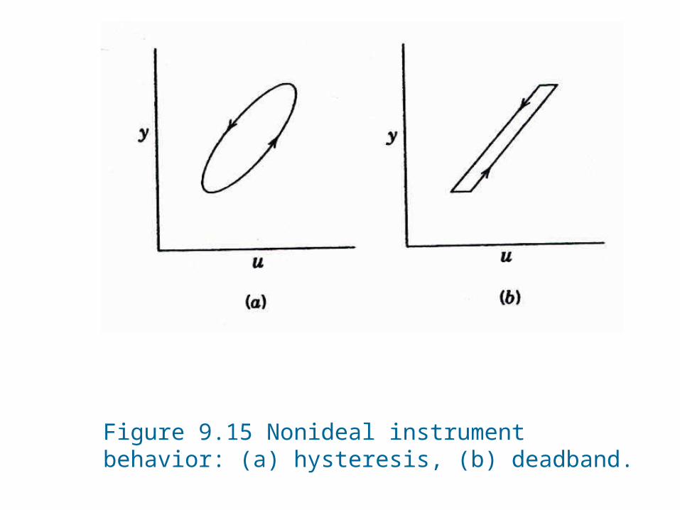
Figure 9.15 Nonideal instrument behavior: (a) hysteresis, (b) deadband.

• Example:Example: Flow Control Loop

Assume FT is direct-acting.

1. Air-to-open (fail close) valve ==> ?2. Air-to-close (fail open) valve ==> ?

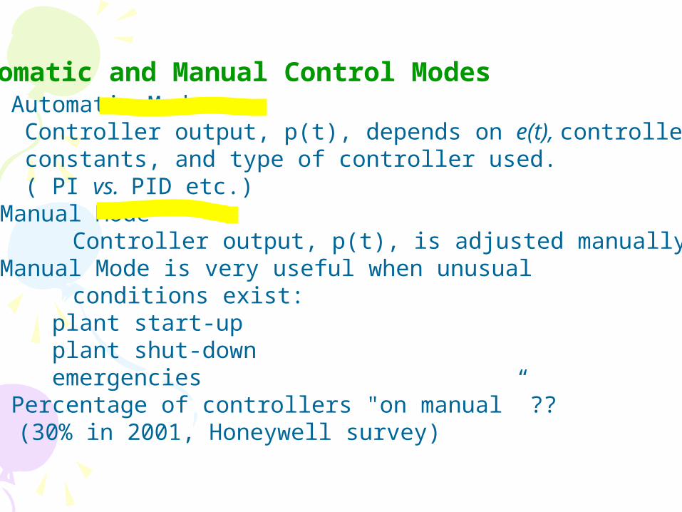
Automatic and Manual Control Modes• Automatic Mode

Controller output, p(t), depends on e(t), controller constants, and type of controller used. ( PI vs. PID etc.)

Manual Mode Controller output, p(t), is adjusted manually. Manual Mode is very useful when unusual conditions exist:

plant start-upplant shut-downemergencies

• Percentage of controllers "on manual” ?? (30% in 2001, Honeywell survey)

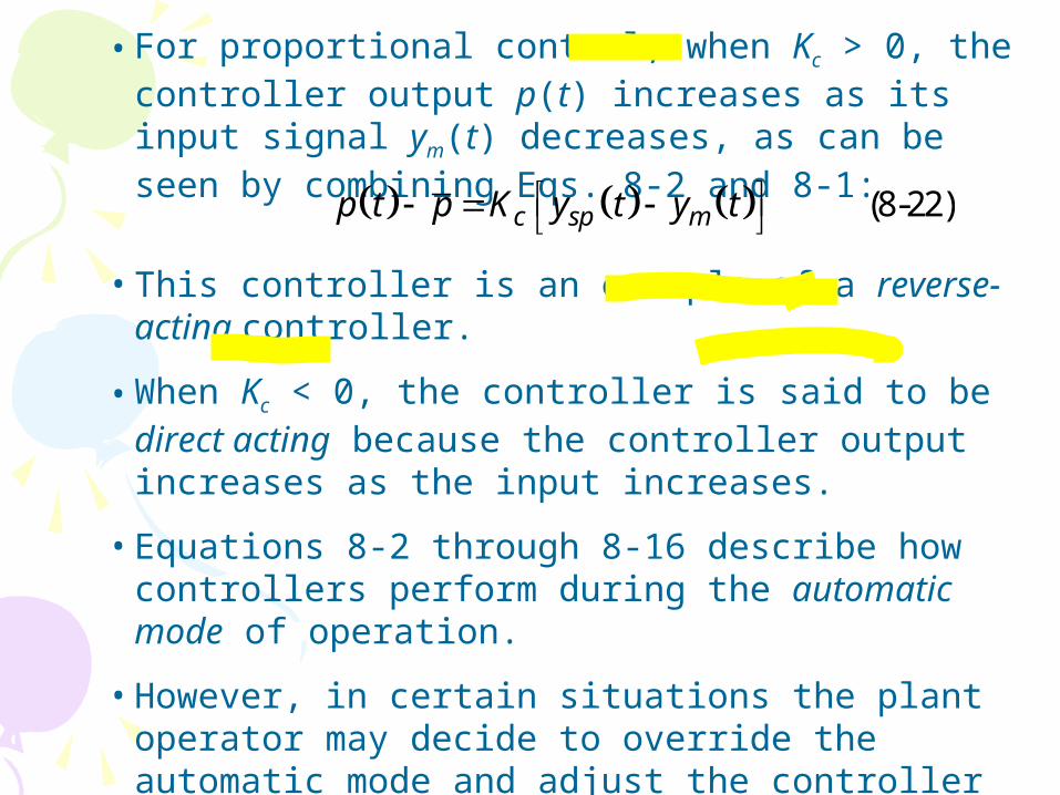
• For proportional control, when Kc > 0, the controller output p(t) increases as its input signal ym(t) decreases, as can be seen by combining Eqs. 8-2 and 8-1:

(8-22)c sp mp t p K y t y t

• This controller is an example of a reverse-acting controller.

• When Kc < 0, the controller is said to be direct acting because the controller output increases as the input increases.

• Equations 8-2 through 8-16 describe how controllers perform during the automatic mode of operation.

• However, in certain situations the plant operator may decide to override the automatic mode and adjust the controller output manually.

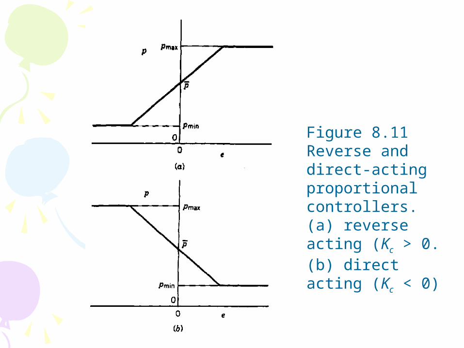
Figure 8.11 Reverse and direct-acting proportional controllers. (a) reverse acting (Kc > 0. (b) direct acting (Kc < 0)

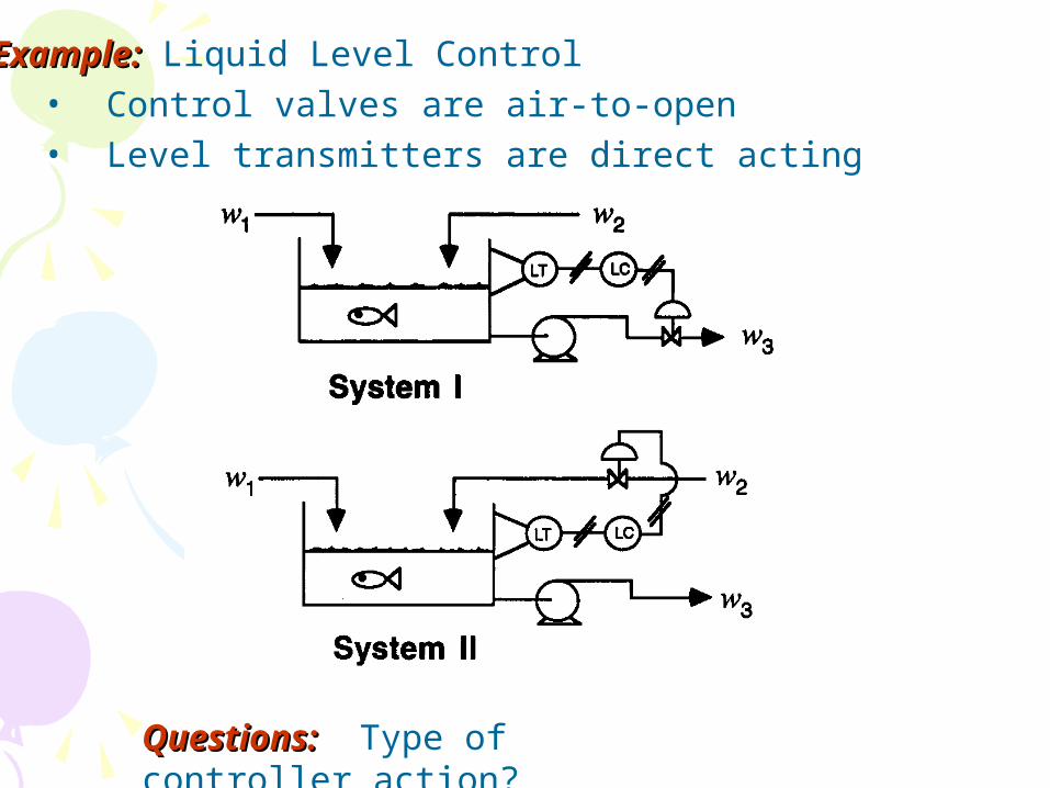
Example:Example: Liquid Level Control• Control valves are air-to-open• Level transmitters are direct acting

Questions:Questions: Type of controller action?

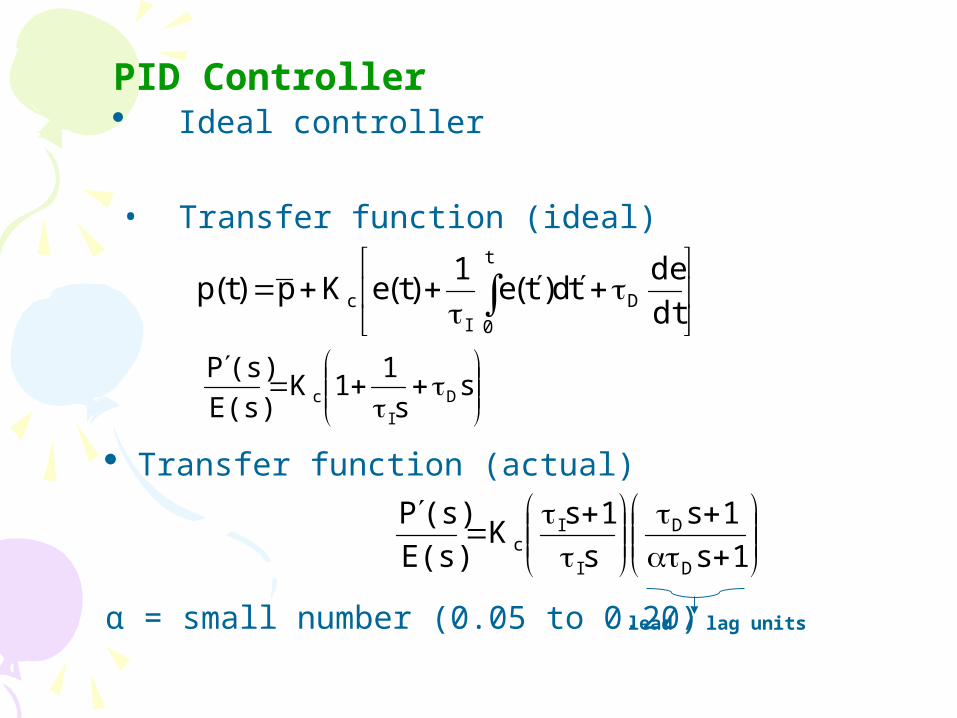
PID Controller Ideal controller

t

0

DI

c dt

detd)t(e

1)t(eKp)t(p

s

s

11K

E(s)

(s)PD

Ic

• Transfer function (ideal)

Transfer function (actual)

α = small number (0.05 to 0.20)

1s

1s

s

1sK

E(s)

(s)P

D

D

I

Ic

lead / lag units

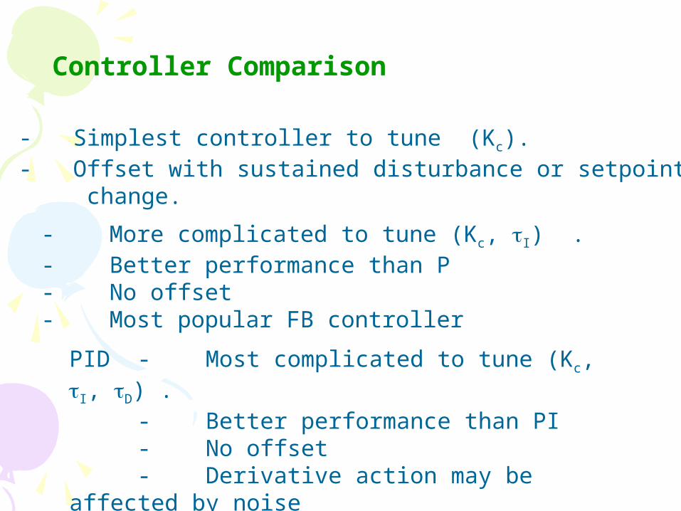
PID - Most complicated to tune (Kc, I, D) .- Better performance than PI- No offset- Derivative action may be affected by noise

PI - More complicated to tune (Kc, I) .- Better performance than P- No offset- Most popular FB controller

P - Simplest controller to tune (Kc).- Offset with sustained disturbance or setpoint change.

Controller Comparison

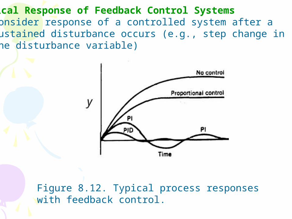
Typical Response of Feedback Control SystemsConsider response of a controlled system after a sustained disturbance occurs (e.g., step change in the disturbance variable)

Figure 8.12. Typical process responses with feedback control.

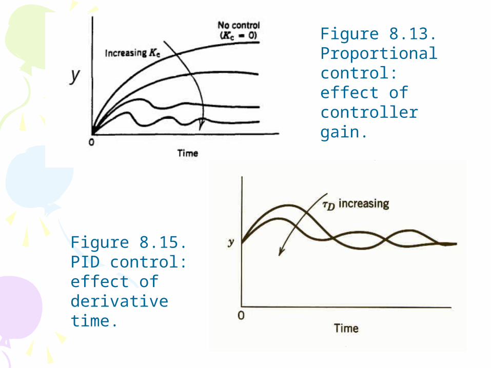
Figure 8.13. Proportional control: effect of controller gain.

Figure 8.15. PID control: effect of derivative time.

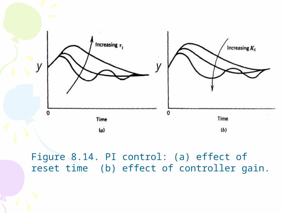
Figure 8.14. PI control: (a) effect of reset time (b) effect of controller gain.

Ch

apte

r 8

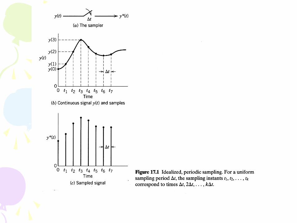
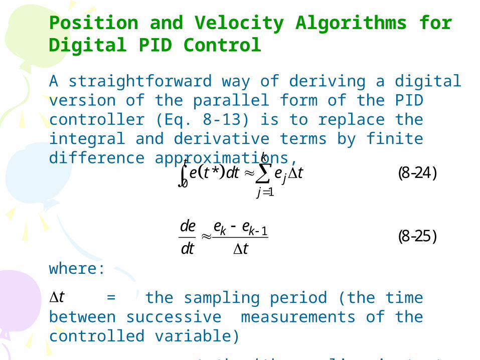
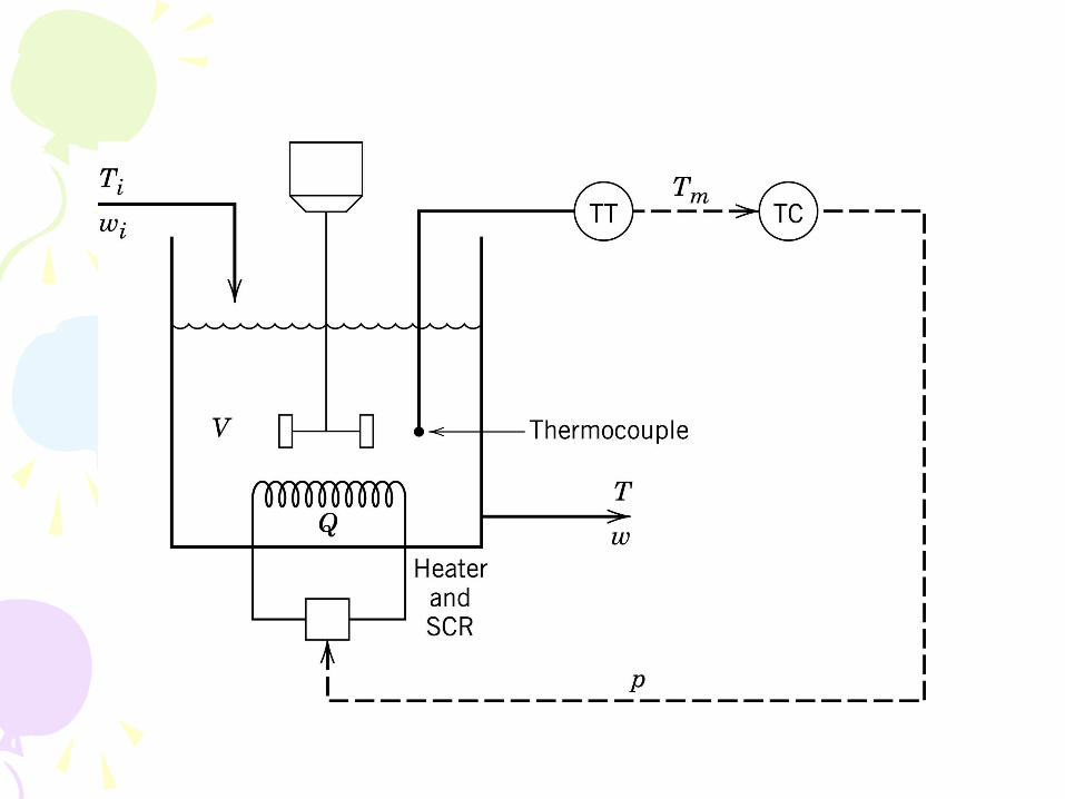
Position and Velocity Algorithms for Digital PID Control

A straightforward way of deriving a digital version of the parallel form of the PID controller (Eq. 8-13) is to replace the integral and derivative terms by finite difference approximations,

0

1

* (8-24)kt

jj

e t dt e t

1 (8-25)k ke ede

dt t

where:

= the sampling period (the time between successive measurements of the controlled variable)

ek = error at the kth sampling instant for k = 1, 2, …

t

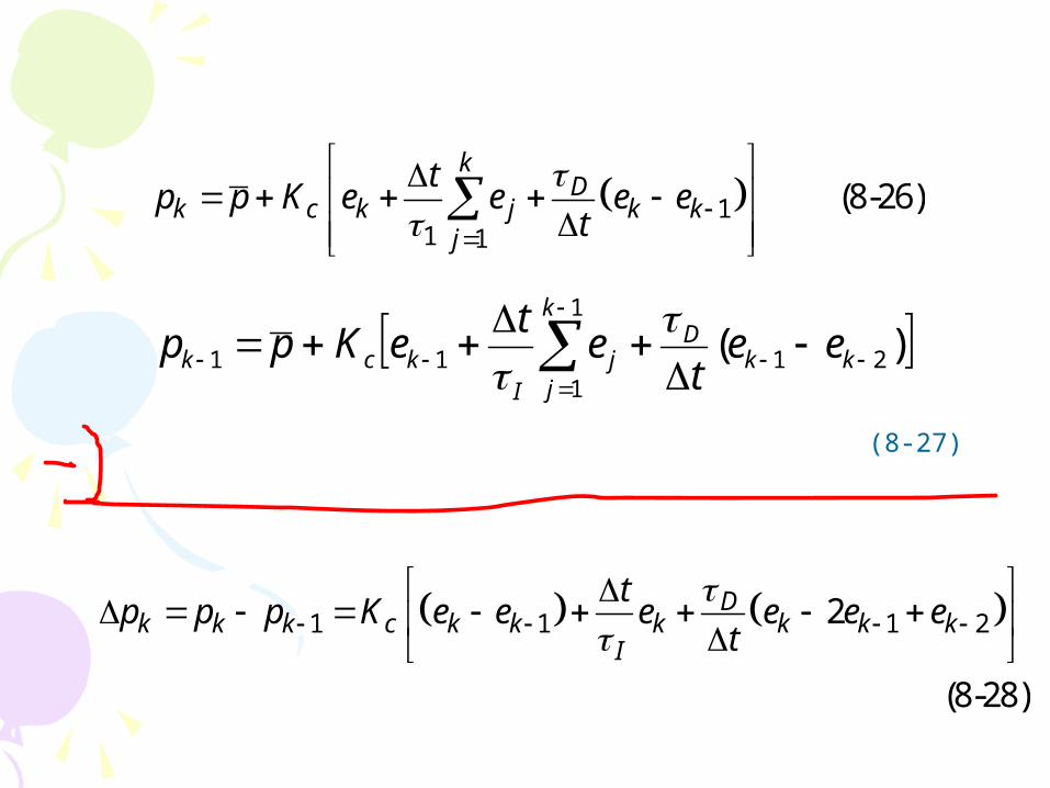
There are two alternative forms of the digital PID control equation, the position form and the velocity form. Substituting (8-24) and (8-25) into (8-13), gives the position form,

11 1

(8-26)k

Dk c k j k k

j

tp p K e e e e

t

Where pk is the controller output at the kth sampling instant. The other symbols in Eq. 8-26 have the same meaning as in Eq. 8-13. Equation 8-26 is referred to as the position form of the PID control algorithm because the actual value of the controller output is calculated.

(8-27)

Note that the summation still begins at j = 1 because it is assumed that the process is at the desired steady state for

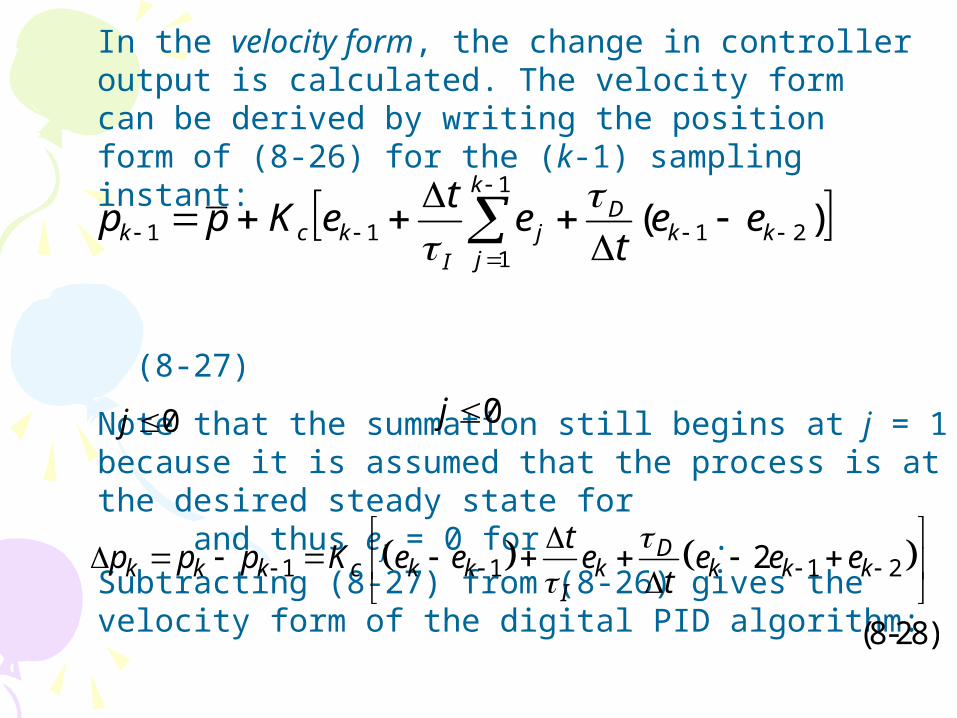
and thus ej = 0 for . Subtracting (8-27) from (8-26) gives the velocity form of the digital PID algorithm:

In the velocity form, the change in controller output is calculated. The velocity form can be derived by writing the position form of (8-26) for the (k-1) sampling instant:

0j 0j

1 1 1 22

(8-28)

Dk k k c k k k k k k

I

tp p p K e e e e e e

t

)( 21

1

111

kk

Dk

jj

Ikck ee

te

teKpp

)( 21

1

111

kk

Dk

jj

Ikck ee

te

teKpp

11 1

(8-26)k

Dk c k j k k

j

tp p K e e e e

t

1 1 1 22

(8-28)

Dk k k c k k k k k k

I

tp p p K e e e e e e

t

(8-27)

The velocity form has three advantages over the position form:

1. It inherently contains anti-reset windup because the summation of errors is not explicitly calculated.

2. This output is expressed in a form, , that can be utilized directly by some final control elements, such as a control valve driven by a pulsed stepping motor.

3. For the velocity algorithm, transferring the controller from manual to automatic mode does not require any initialization of the output ( in Eq. 8-26). However, the control valve (or other final control element) should be placed in the appropriate position prior to the transfer.

kp

p

TransmittersTransmitters

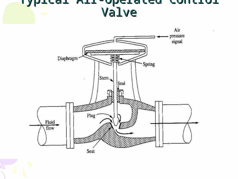
Typical Air-Operated Control ValveTypical Air-Operated Control Valve

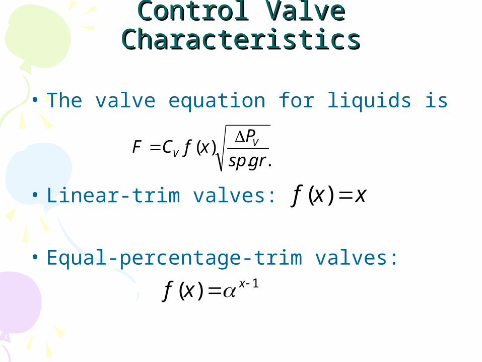
Control Valve CharacteristicsControl Valve Characteristics

• The valve equation for liquids is

• Linear-trim valves:

• Equal-percentage-trim valves:

..)(

grsp

PxfCF V

V

xxf )(

1)( xxf

Control Valve CharacteristicsControl Valve Characteristics

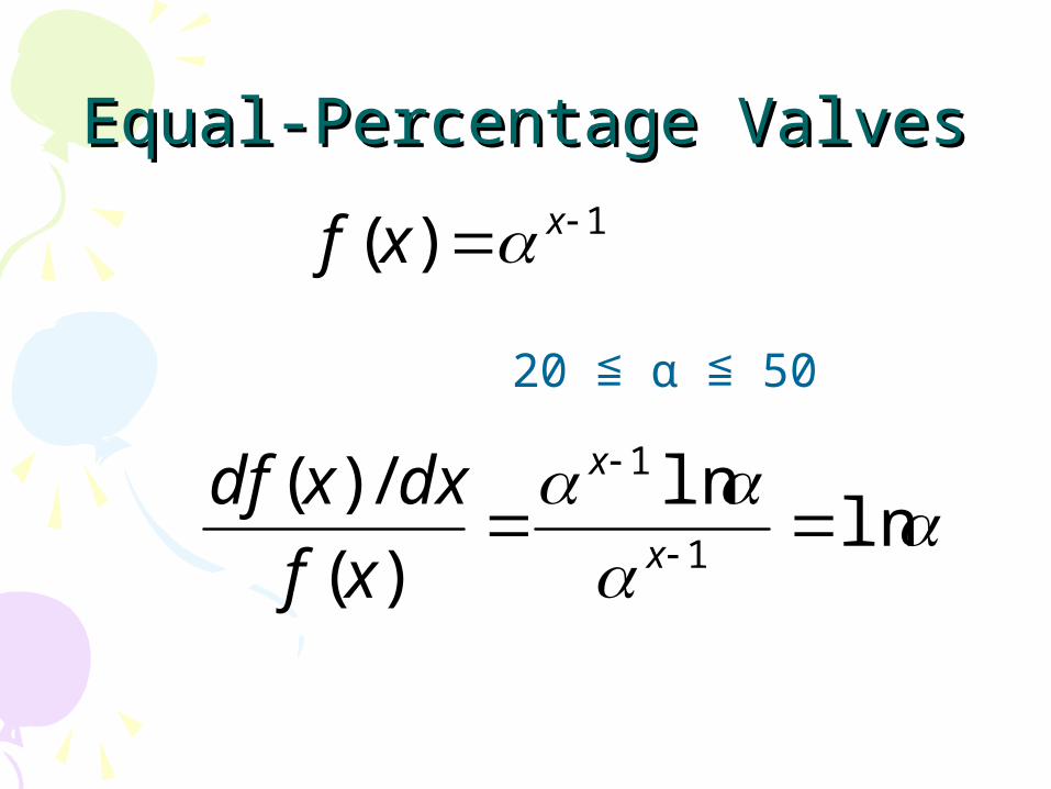
Equal-Percentage ValvesEqual-Percentage Valves

20 ≦ α ≦ 50

1)( xxf

ln

ln

)(

/)(1

1

x

x

xf

dxxdf

Installed CharacteristicsInstalled Characteristics

Installed CharacteristicsInstalled Characteristics