CONTROL ORIENTED MODELING OF AN AUTOMOTIVE … › ~mahdi › Docs › P_Reddy_MScThesis.pdf ·...
187
CONTROL ORIENTED MODELING OF AN AUTOMOTIVE DRIVETRAIN FOR ANTI-JERK CONTROL By Gurijala Venkat Prithvi Reddy A THESIS Submitted in partial fulfillment of the requirements for the degree of MASTER OF SCIENCE In Mechanical Engineering MICHIGAN TECHNOLOGICAL UNIVERSITY 2018 2018 Gurijala Venkat Prithvi Reddy
Transcript of CONTROL ORIENTED MODELING OF AN AUTOMOTIVE … › ~mahdi › Docs › P_Reddy_MScThesis.pdf ·...

CONTROL ORIENTED MODELING OF AN AUTOMOTIVE DRIVETRAIN
FOR ANTI-JERK CONTROL
By
Gurijala Venkat Prithvi Reddy
A THESIS
Submitted in partial fulfillment of the requirements for the degree of
MASTER OF SCIENCE
In Mechanical Engineering
MICHIGAN TECHNOLOGICAL UNIVERSITY
2018
© 2018 Gurijala Venkat Prithvi Reddy


This thesis has been approved in partial fulfillment of the requirements for the Degree
of MASTER OF SCIENCE in Mechanical Engineering.
Department of Mechanical Engineering - Engineering Mechanics
Thesis Advisor: Dr. Mahdi Shahbakhti
Thesis Co-advisor: Dr. Darrell Robinette
Committee Member: Dr. Jason Blough
Committee Member: Dr. Jeremy Worm
Committee Member:
Committee Member:
Department Chair: Dr. William W. Predebon

Contents
List of Figures . . . . . . . . . . . . . . . . . . . . . . . . . . . . . . . . . ix
List of Tables . . . . . . . . . . . . . . . . . . . . . . . . . . . . . . . . . . xvii
Acknowledgments . . . . . . . . . . . . . . . . . . . . . . . . . . . . . . . xix
Nomenclature . . . . . . . . . . . . . . . . . . . . . . . . . . . . . . . . . . xxi
List of Abbreviations . . . . . . . . . . . . . . . . . . . . . . . . . . . . . xxv
Abstract . . . . . . . . . . . . . . . . . . . . . . . . . . . . . . . . . . . . . xxvii
1 Introduction . . . . . . . . . . . . . . . . . . . . . . . . . . . . . . . . . 1
1.1 Motivation . . . . . . . . . . . . . . . . . . . . . . . . . . . . . . . . 1
1.2 Technical terms used in this work . . . . . . . . . . . . . . . . . . . 6
1.3 Literature review . . . . . . . . . . . . . . . . . . . . . . . . . . . . 11
1.3.1 Driveline modeling . . . . . . . . . . . . . . . . . . . . . . . 11
1.3.2 AJC state estimators and parameter observers . . . . . . . . 16
1.3.3 AJC torque shaping controllers . . . . . . . . . . . . . . . . 21
1.4 Research scope and Thesis organization . . . . . . . . . . . . . . . . 24
v

2 Full order model development and validation . . . . . . . . . . . . 27
2.1 Model development . . . . . . . . . . . . . . . . . . . . . . . . . . . 27
2.1.1 Amesim® and Simulink® interface . . . . . . . . . . . . . . 28
2.1.2 Model assumptions and limitations . . . . . . . . . . . . . . 32
2.1.3 Engine model . . . . . . . . . . . . . . . . . . . . . . . . . . 33
2.1.4 Driveline and vehicle dynamics model . . . . . . . . . . . . . 36
2.1.4.1 Torque converter model . . . . . . . . . . . . . . . 37
2.1.4.2 Automatic transmission model . . . . . . . . . . . 40
2.1.4.3 Propeller shaft model . . . . . . . . . . . . . . . . 43
2.1.4.4 Final drive model . . . . . . . . . . . . . . . . . . . 43
2.1.4.5 Backlash model . . . . . . . . . . . . . . . . . . . . 44
2.1.4.6 Axle shafts model . . . . . . . . . . . . . . . . . . 46
2.1.4.7 Suspension, tire and vehicle dynamics model . . . . 47
2.2 Model validation . . . . . . . . . . . . . . . . . . . . . . . . . . . . 52
2.2.1 Case 1: Torque converter lock-up clutch locked . . . . . . . 55
2.2.1.1 Sub-case 1: Original vehicle parameters . . . . . . 55
2.2.1.2 Sub-case 2: Modified vehicle parameters - Vehicle
mass increased . . . . . . . . . . . . . . . . . . . . 59
2.2.1.3 Sub-case 3: Effect of engine accessory load . . . . . 61
2.2.1.4 Sub-case 4: Using crankshaft torque signal from ex-
perimental data . . . . . . . . . . . . . . . . . . . . 63
vi

2.2.1.5 Sub-case 5: Modified coefficient of rolling resistance 66
2.2.1.6 Sub-case 6: Propeller and axle shaft stiffness reduced 69
2.2.1.7 Sub-case 7: Engine, torque converter, and transmis-
sion inertia adjusted . . . . . . . . . . . . . . . . . 70
2.2.1.8 Sub-case 8: Implementation of filter for propeller shaft
torque . . . . . . . . . . . . . . . . . . . . . . . . . 73
2.2.2 Case 2: Torque converter lock-up clutch open . . . . . . . . 75
2.2.3 Case 3: Torque converter lock-up clutch slipping . . . . . . . 78
3 Parametric Analysis of Driveline Response . . . . . . . . . . . . . 83
3.1 Effect of varying input torque ramp rate . . . . . . . . . . . . . . . 84
3.1.1 Tip-in scenarios . . . . . . . . . . . . . . . . . . . . . . . . . 84
3.1.1.1 With backlash in positive contact and TCC locked 85
3.1.1.2 With backlash in negative contact and TCC locked 88
3.1.1.3 With backlash in negative contact and TCC slipping 92
3.1.2 Tip-out scenarios . . . . . . . . . . . . . . . . . . . . . . . . 94
3.1.2.1 With backlash in positive contact and TCC locked 94
3.1.2.2 With backlash in negative contact and TCC locked 95
3.1.2.3 With backlash in negative contact and TCC open . 95
3.1.3 During backlash traversal . . . . . . . . . . . . . . . . . . . 98
3.2 Effect of varying backlash size . . . . . . . . . . . . . . . . . . . . . 101
3.2.1 Variation in transmission backlash . . . . . . . . . . . . . . 101
vii

3.2.2 Variation in final drive backlash . . . . . . . . . . . . . . . . 102
3.3 Effect of varying propeller and axle shaft properties . . . . . . . . . 105
3.3.1 Effect of varying propeller shaft stiffness . . . . . . . . . . . 105
3.3.2 Effect of varying axle shaft stiffness . . . . . . . . . . . . . . 106
3.4 Effect of varying propeller and axle shaft damping coefficient . . . . 110
4 Reduced-order model (ROM): Development and validation . . . 113
4.1 Introduction . . . . . . . . . . . . . . . . . . . . . . . . . . . . . . . 113
4.2 ROM with lumped tire parameters . . . . . . . . . . . . . . . . . . 115
4.2.1 ROM I development . . . . . . . . . . . . . . . . . . . . . . 115
4.2.2 ROM I validation . . . . . . . . . . . . . . . . . . . . . . . . 117
4.3 ROM with separate tire parameters . . . . . . . . . . . . . . . . . . 119
4.3.1 ROM II development . . . . . . . . . . . . . . . . . . . . . . 119
4.3.2 ROM II validation . . . . . . . . . . . . . . . . . . . . . . . 122
4.3.3 Effect of lumping backlashes in the ROM . . . . . . . . . . . 122
4.4 Estimation of model parameters for ROM . . . . . . . . . . . . . . 126
4.5 Application of ROM for controls . . . . . . . . . . . . . . . . . . . . 128
5 Conclusion and Future work . . . . . . . . . . . . . . . . . . . . . . 133
5.1 Conclusions . . . . . . . . . . . . . . . . . . . . . . . . . . . . . . . 133
5.2 Future work . . . . . . . . . . . . . . . . . . . . . . . . . . . . . . . 137
References . . . . . . . . . . . . . . . . . . . . . . . . . . . . . . . . . . . . 139
viii

A Amesim-Simulink Interface . . . . . . . . . . . . . . . . . . . . . . . 147
B Engine Torque Uncertainty . . . . . . . . . . . . . . . . . . . . . . . 149
C Program and Data File Summary . . . . . . . . . . . . . . . . . . . 153
C.1 Chapter 1 . . . . . . . . . . . . . . . . . . . . . . . . . . . . . . . . 153
C.2 Chapter 2 . . . . . . . . . . . . . . . . . . . . . . . . . . . . . . . . 154
C.3 Chapter 3 . . . . . . . . . . . . . . . . . . . . . . . . . . . . . . . . 155
C.4 Chapter 4 . . . . . . . . . . . . . . . . . . . . . . . . . . . . . . . . 156
C.5 Appendix B . . . . . . . . . . . . . . . . . . . . . . . . . . . . . . . 157
ix


List of Figures
1.1 Segment wise sale of new automobiles in the United States in 2016 [1]. 2
1.2 Projected vehicle sales in American, European and Chinese markets
between 2017 - 2030, classified based on propulsion technology [2]. . 3
1.3 Projected sales of autonomous vehicles in American, European, and
Chinese markets between 2017 - 2030, classified by the level of au-
tomation [3]. . . . . . . . . . . . . . . . . . . . . . . . . . . . . . . . 4
1.4 Motivation behind the current research. . . . . . . . . . . . . . . . . 6
1.5 Backlash in gears [4]. . . . . . . . . . . . . . . . . . . . . . . . . . . 7
1.6 Representative output of propeller shaft torque showing clunk and
shuffle, and backlash traversal in driveline. . . . . . . . . . . . . . . 10
1.7 Timeline of some of the prior AJC works in research literature. . . . 14
1.8 Some of the estimator design approaches used in the AJC
literature[5][6][7][8][9]. . . . . . . . . . . . . . . . . . . . . . . . . . 20
1.9 Some of the torque shaping controller design approaches given in the
AJC literature[10][11][12]. . . . . . . . . . . . . . . . . . . . . . . . 22
1.10 Thesis organization . . . . . . . . . . . . . . . . . . . . . . . . . . . 26
xi

2.1 Components of the full-order model. Top box represents components
modeled in Simulink, and bottom box represents components modeled
in Amesim. . . . . . . . . . . . . . . . . . . . . . . . . . . . . . . . 29
2.2 Overview of Amesim® - Simulink® interface. Adapted from [13]. . 31
2.3 Amesim® model showing the torque converter with lock-up clutch and
spring hysteresis blocks. . . . . . . . . . . . . . . . . . . . . . . . . 38
2.4 Schematic diagram showing the 10-speed transmission[14]. . . . . . 41
2.5 Amesim® model showing the 10-speed automatic transmission
blocks. . . . . . . . . . . . . . . . . . . . . . . . . . . . . . . . . . . 42
2.6 Representative model of backlash. . . . . . . . . . . . . . . . . . . . 45
2.7 Amesim® model showing the propeller and axle shafts, along with the
rear differential and final drive backlash. . . . . . . . . . . . . . . . 46
2.8 Amesim® model showing the suspension, tire and the vehicle dynam-
ics blocks. . . . . . . . . . . . . . . . . . . . . . . . . . . . . . . . . 49
2.9 Overview of the Amesim® vehicle model. . . . . . . . . . . . . . . 51
2.10 Overview of the model validation work done. . . . . . . . . . . . . . 53
2.11 Results for sub-case 1 of model validation: Compar-
ison between experimental and simulation data with
initial driveline parameters(Table 2.2). . . . . . . . . . . . . . . . . 57
2.12 Results for sub-case 2 of model validation: Comparison between exper-
imental and simulation data with increased vehicle mass(Table 2.4). 60
xii

2.13 Results for sub-case 3 of model validation: Comparison between ex-
perimental and simulation data after increasing vehicle mass, and
subtracting engine accessory load torque(Table 2.6). . . . . . . . . . 62
2.14 Results for sub-case 4 of model validation: Comparison between ex-
perimental and simulation data with experimental crankshaft torque
trajectory as input. . . . . . . . . . . . . . . . . . . . . . . . . . . . 65
2.15 Results for sub-case 5 of model validation: Compar-
ison between experimental and simulation data with
reduced coefficient of rolling resistance(Table 2.10. . . . . . . . . . . 68
2.16 Results for sub-case 6 of model validation: Compar-
ison between experimental and simulation data with
reduced axle and propeller shaft stiffness(Table 2.12). . . . . . . . . 71
2.17 Results for sub-case 7 of model validation: Comparison be-
tween experimental and simulation data with crankshaft
torque as input, reduced vehicle mass, reduced coeffi-
cient of rolling resistance, reduced drive shaft stiffness, and
increased inertia of engine, torque converter and transmission(Table 2.14). 74
xiii

2.18 Simulation output in 5th gear with estimated crankshaft torque com-
pensated for error as input to Amesim®, modified vehicle mass, mod-
ified coefficient of rolling resistance, modified propeller shaft and axle
shaft stiffness, and modified engine, torque converter and transmission
inertia, and filtered driveshaft torque. . . . . . . . . . . . . . . . . . 76
2.19 Results for the case of open torque converter clutch. Comparison be-
tween experimental and simulation data with adjusted parameters from
previous section, with TCC status open(Table 2.16). . . . . . . . . . 79
2.20 Results for the case of slipping torque converter clutch. Comparison
between experimental and simulation data, with adjusted parameters
from previous section, and with TCC status slipping(Table 2.17). . 81
3.1 Driveline response for tip-in scenario with 150 Nm/s ramp rate, back-
lash in positive contact, and locked TCC. . . . . . . . . . . . . . . . 86
3.2 Driveline response for tip-in scenario with 500 Nm/s ramp rate, back-
lash in positive contact, and locked TCC. . . . . . . . . . . . . . . . 87
3.3 Driveline response for tip-in scenario with 150 Nm/s ramp rate, back-
lash in negative contact, and locked TCC. . . . . . . . . . . . . . . 90
3.4 Driveline response for tip-in scenario with 500 Nm/s ramp rate, back-
lash in negative contact, and locked TCC. . . . . . . . . . . . . . . 91
3.5 Driveline response for tip-in scenario with 500 Nm/s ramp rate, back-
lash in negative contact, and slipping TCC. . . . . . . . . . . . . . 93
xiv

3.6 Driveline response for tip-out scenario with 150 Nm/s ramp rate, back-
lash in positive contact, and locked TCC. . . . . . . . . . . . . . . . 96
3.7 Driveline response for tip-out scenario with 150 Nm/s ramp rate, back-
lash in negative contact, and locked TCC. . . . . . . . . . . . . . . 97
3.8 Driveline response for tip-out scenario with 150 Nm/s ramp rate, back-
lash in negative contact, and open TCC. . . . . . . . . . . . . . . . 99
3.9 Driveline response for tip-in scenario with torque ramp rate varying
during backlash traversal. The backlash is initially in negative contact,
and TCC is locked. . . . . . . . . . . . . . . . . . . . . . . . . . . . 100
3.10 Effect of changing the transmission backlash on driveline response.
Case A represents condition where transmission backlash is 10 deg.
Case B represents condition where transmission backlash is 20 deg. 103
3.11 Effect of increasing the final drive backlash on driveline response. Case
A represents condition where final drive backlash is 4 deg. Case B
represents condition where final drive backlash is 8 deg. . . . . . . . 104
3.12 Effect of changing propeller shaft stiffness on overall driveline response.
Case A represents condition where propeller shaft stiffness is decreased
by 25%. Case B represents condition where propeller shaft stiffness is
increased by 25%. . . . . . . . . . . . . . . . . . . . . . . . . . . . . 107
xv

3.13 Effect of changing axle shaft stiffness on overall driveline response.
Case A represents condition where axle shaft stiffness is increased by
25%. Case B represents condition where axle shaft stiffness is decreased
by 25%. . . . . . . . . . . . . . . . . . . . . . . . . . . . . . . . . . 109
3.14 Effect of changing axle shaft damping on driveline response. Case A
represents condition where axle shaft damping is increased by 25%.
Case B represents condition where axle shaft damping is decreased by
25%. . . . . . . . . . . . . . . . . . . . . . . . . . . . . . . . . . . . 111
4.1 ROM with lumped tire parameters. . . . . . . . . . . . . . . . . . . 116
4.2 Comparison of ROM Iwith lumped tire parameters’ driveline response
with FOM, for a tip-in scenario. . . . . . . . . . . . . . . . . . . . . 118
4.3 ROM with separate tire parameters. . . . . . . . . . . . . . . . . . 119
4.4 Comparison of ROM IIwith separate tire parameters’ driveline re-
sponse with FOM, for a tip-in scenario. . . . . . . . . . . . . . . . . 121
4.5 Comparison of ROM with separate tire parameters’ driveline response
with FOM, in 3rd gear, for a tip-in scenario. . . . . . . . . . . . . . 123
4.6 Comparison of lumped and split backlash models in full-order and
reduced-order models. . . . . . . . . . . . . . . . . . . . . . . . . . 125
4.7 Schematic showing a simple control system, utilizing the output of
the ROM, for controlling the torque delivered to the plant(Full-order
model). . . . . . . . . . . . . . . . . . . . . . . . . . . . . . . . . . 128
xvi

4.8 Comparison of driveline response for two cases of torque input. Case
A: Torque input without shaping. Case B: Torque input with shaping. 131
B.1 Observed engine torque response for a throttle input of 0 → 100% . 150
B.2 Observed engine torque response for a throttle input of 0 → 60% . 150
B.3 Observed engine torque response for a throttle input of 0 → 20% . 151
B.4 Observed response for a throttle tip-out scenario . . . . . . . . . . . 151
xvii


List of Tables
2.1 Frequency of driveline oscillations in sub-case 1 . . . . . . . . . . . 56
2.2 Simulation parameters for Case 1 . . . . . . . . . . . . . . . . . . . 58
2.3 Frequency of driveline oscillations in sub-case 2 . . . . . . . . . . . 59
2.4 Simulation parameters for Case 2 . . . . . . . . . . . . . . . . . . . 59
2.5 Frequency of driveline oscillations in sub-case 3 . . . . . . . . . . . 61
2.6 Simulation parameters for sub-case 3 . . . . . . . . . . . . . . . . . 63
2.7 Frequency of driveline oscillations in sub-case 4 . . . . . . . . . . . 64
2.8 Simulation parameters for sub-case 4 . . . . . . . . . . . . . . . . . 64
2.9 Frequency of driveline oscillations in sub-case 5 . . . . . . . . . . . 67
2.10 Simulation parameters for sub-case 5 . . . . . . . . . . . . . . . . . 67
2.11 Frequency of driveline oscillations in sub-case 6 . . . . . . . . . . . 70
2.12 Simulation parameters for sub-case 6 . . . . . . . . . . . . . . . . . 72
2.13 Frequency of driveline oscillations in sub-case 7 . . . . . . . . . . . 73
2.14 Simulation parameters for sub-case 7 . . . . . . . . . . . . . . . . . 73
2.15 Filter parameters used for filtering simulated propeller shaft torque 75
2.16 Simulation parameters for Case 2: TCC open condition . . . . . . . 78
xix

2.17 Simulation parameters for Case 3: TCC slipping condition . . . . . 80
C.1 Chapter 1 figure files . . . . . . . . . . . . . . . . . . . . . . . . . . 153
C.2 Chapter 2 figure files . . . . . . . . . . . . . . . . . . . . . . . . . . 154
C.3 Chapter 2 model files . . . . . . . . . . . . . . . . . . . . . . . . . . 154
C.4 Chapter 2 model validation files . . . . . . . . . . . . . . . . . . . . 155
C.5 Chapter 3 figure files . . . . . . . . . . . . . . . . . . . . . . . . . . 155
C.6 Chapter 3 model files . . . . . . . . . . . . . . . . . . . . . . . . . . 156
C.7 Chapter 4 figure files . . . . . . . . . . . . . . . . . . . . . . . . . . 156
C.8 Chapter 4 model files . . . . . . . . . . . . . . . . . . . . . . . . . . 157
C.9 Appendix B figure files . . . . . . . . . . . . . . . . . . . . . . . . . 157
xx

Acknowledgments
This work would not have been possible without the excellent guidance, and patient
support of Dr. Mahdi Shahbakhti, and Dr. Darrell Robinette. Their mentorship has
taught me invaluable lessons, in subject and life, for which I am grateful to them.
I would like to thank Dr. Maruthi Ravichandran, and Dr. Jeffrey Doering, of Ford
Motor Company, for their valuable technical insights, and patience during the many
meetings that took place through the course of this work. Thanks are also due to
Vehicle Controls and Systems Engineering (VCSE) department of Ford Research and
Advanced (R&A) Engineering Organization. I would like to thank Mary Farmer
(Technical Expert, Ford Motor Co.), for her help with experimental data collection,
and inputs towards making this project better. I would also like to thank Imad
Khan, Hsun-Hsuan Huang, Vladimir Ivanovic, Dan Nagelhout, Natalie Remisoski,
and Kalyan Addepalli for their help in obtaining vehicle parameters.
I am grateful to Dr. Jason Blough and Dr. Jeremy Worm, for accepting to be on my
thesis defense committee and for their support in the weeks preceding my defense.
Their feedback on this work will help in improving the future work of this project.
I graciously acknowledge Prince Lakhani and Kaushal Darokar for their contributions,
and for the meaningful discussions that took place during the course of this project.
xxi

Thanks are also due to my roommates Sampath Rallapalli, and Vishnu Durgam, who
helped in creating a lively, fun-filled atmosphere at home.
I owe everything in my life to the love, and support I received from my parents,
Radha and Prakash, and my family members, Kedar, and Hasitha. Their belief in
my abilities has always motivated me to be a better person, and for that I can not
thank them enough.
xxii

Nomenclature
α Backlash angle [deg.]
δ Road slope for use in longitudinal vehicle dynamics [rad]
θax Angular position of axle shaft [rad]
θb Angular position of backlash [rad]
θe Angular position of the engine [rad]
θs Angular position of shaft [rad]
θt Angular position of transmission output shaft [rad]
θps Angular position of propeller shaft at final drive end [rad]
θti Angular position of tire [rad]
θax Angular speed of axle shaft at tire end [rad/s]
θe Angular speed of the engine [rad/s]
θps Angular speed of propeller shaft at final drive end [rad/s]
θti Angular speed of tire [rad/s]
θtr Angular speed of transmission output shaft [rad/s]
θw Angular speed of wheel hub [rad/s]
θe Angular acceleration of the engine [rad/s2]
aveh Longitudinal acceleration of the vehicle [m/s2]
Af Frontal area of the vehicle [m2]
xxiii
CD Coefficient of drag [−]
cax Damping of the axle shaft [N.m/RPM ]
cps Damping of the propeller shaft [N.m/RPM ]
cs Damping of shaft [N.m/RPM ]
cti Damping of the tire [N.m/RPM ]
F Multiplication factor used in section 4.5 [−]
Faero Aerodynamic force on the vehicle [N ]
Fengine Propulsive force developed by the engine [N ]
Froll Rolling resistance force on the vehicle [N ]
Fslope Slope force on the vehicle [N ]
g Acceleration due to gravity [m/s2]
itr Gear ratio of current gear state of the transmission [−]
ifd Gear ratio of the final drive[−]
Je Rotational inertia of the engine [kg.m2]
Jw Rotational inertia of the wheel hub [kg.m2]
K Capacity factor of torque converter [RPM/√N.m]
kax Stiffness of the axle shaft [N.m/deg]
kps Stiffness of the propeller shaft [N.m/deg]
ks Stiffness of shaft [N.m/deg]
kti Stiffness of the tire [N.m/deg]
N Engine speed [RPM ]
xxiv

rveh Coefficient of viscous friction [−]
rti Radius of the tire [m]
SR Speed ratio of torque converter [−]
t Time [sec]
τe,base Time constant of first-order lag [msec]
t(d,base) Time delay in base path [sec]
t(d,inst) Time delay in instantaneous path [sec]
Tax Torque output from axle shaft [N.m]
Tdriver Driver requested torque [N.m]
Tfric Friction losses of engine torque [N.m]
TRspk Torque ratio due to spark modulation [−]
Tfd Torque output from final drive [N.m]
Tim Torque input at torque converter impeller [N.m]
Tps Torque output from propeller shaft [N.m]
Tshaped Shaped engine torque output in ROM [N.m]
Ttcc Torque through the torque converter lock-up clutch [N.m]
Tti Torque output at the tire [N.m]
Ttu Torque output at torque converter turbine [N.m]
Ttr Torque output from transmission [N.m]
Tgearloss Torque loss inside the transmission [N.m]
TR Torque ratio of torque converter [−]
xxv

Tunc Uncertainty in engine delivered torque [N.m]
V Velocity of the vehicle [m/s]
Vwind Wind velocity acting on the vehicle [m/s]
xxvi

List of Abbreviations
2WD Two Wheel Drive
4WD Four Wheel Drive
AT Automatic Transmission
AJC Anti-Jerk Control
CAN Controller Area Network
CV Constant Velocity
CVT Continuously Variable Transmission
DKF Discrete Kalman Filter
ECU Electronic Control Unit
EKF Extended Kalman Filter
FOM Full Order Model
HEV Hybrid Electric Vehicle
HIL Hardware in Loop
IC Internal Combustion
LO Luenberger Observer
LQR Linear Quadratic Regulator
MT Manual Transmission
MPC Model Predictive Control
xxvii

MPT Multi Parametric Toolbox
NVH Noise Vibration and Harshness
PI Proportional Integrator
PWA Piecewise Affine
ROM Reduced Order Model
SKF Scented Kalman Filter
SMO Sliding Mode Observer
SP Smith Predictor
SUV Sports Utility Vehicle
TCC Torque converter lock-up clutch
TCU Transmission Control Unit
xxviii

Abstract
Drivability is an important metric during the development of an automobile. Cali-
bration engineers spend a significant amount of time trying to improve the drivability
of vehicles for various driving conditions. With an increase in the available compu-
tational power in an automobile, novel model-based methods are being implemented
for further improving the drivability, while reducing calibration time and effort. Phe-
nomenon known as clunk and shuffle, which are caused due to backlash and com-
pliance in the driveline, are a major cause of issues related to drivability and noise,
vibration and harshness (NVH) during tip-in and tip-out scenarios.
This thesis focuses on developing a high-fidelity, control-oriented vehicle driveline
model, which can be used for developing systems, to improve the drivability of a
vehicle, during tip-in and tip-out events. A first principle physics-based model is
developed, which includes the engine as a torque generator, backlash elements as dis-
continuities, and driveshafts as compliant elements. Experimental validation results
showed that the accuracy of the developed model, in representing shuffle oscillation
frequency, during the tip-in scenarios, with locked torque converter clutch, is approx-
imately 99 %.
A parametric analysis is performed to characterize the behavior of the model during
xxix
different input conditions, and to study the effect of backlash size, and driveshaft
compliance on the response of the driveline. Based on the observations from the
parametric analysis, the high-fidelity model is later condensed into a reduced-order
model, and comparative analysis is carried out between two reduced-order model
(ROM) designs. The comparative results between the full-order model and ROM
show that the ROM with separate tire parameters is better in predicting the frequency
and amplitude of shuffle oscillations during tip-in events.
xxx

Chapter 1
Introduction
1.1 Motivation
Ever since the first production automobile was built by Karl Benz in 1885, there
have been plenty of innovations with respect to performance, safety, efficiency and
comfort of an automobile. With the advent of the electronic control unit (ECU)
in automobiles, developments in the automotive industry took new heights. Cars
today have dozens of ECUs on-board to manage tasks as simple as controlling the
headlights, to complicated transient emission control of engines. As the computational
power and reliability of electronic control systems in automobiles increase, it opens
up new avenues for implementing innovative technologies.
1

Figure 1.1: Segment wise sale of new automobiles in the United States in2016 [1].
With crossovers, and pick-up trucks dominating the market share in the United States
(Fig. 1.1), automotive manufacturers are increasingly focusing on refining these seg-
ments, which includes improving the drivability of these vehicles. Drivability can
be defined as the qualitative evaluation of the powertrain’s (interchangeably referred
to as driveline in this thesis) operational characteristics which includes aspects like
smooth acceleration, seamless gear shifts, etc. The current work is motivated by the
need to reduce undesirable jerks that are experienced due to the oscillations induced
into the powertrain, caused by: (i) the presence of backlash within elements of the
driveline like the transmission, final drive, constant velocity (CV) joints etc., and (ii)
the flexibility of axle shafts.
2

Figure 1.2: Projected vehicle sales in American, European and Chinesemarkets between 2017 - 2030, classified based on propulsion technology [2].
While the perception of backlash induced oscillations is subjective, it is also dependent
on factors like the source of propulsion (IC engine, electric motor, hybrid system),
and configuration of the driveline (2WD, 4WD, etc.). With an increase in the sales
of hybrid electric vehicles (HEVs) and electric vehicles (EVs) (Fig. 1.2), the torque
delivery characteristics of an electric motor is playing an important role in determining
the drivability of the vehicle. An IC engine is subject to delays in torque generation
and delivery due to the dynamics of manifold filling and fuel combustion. The electric
motor however, does not have such delays, and therefore, torque generation and
delivery is quite instantaneous, which may lead to higher impact velocities at backlash
zones, causing harsh vibrations throughout the driveline.
Also, with increasing availability of driver-assistance technologies, semi-autonomous
3

Figure 1.3: Projected sales of autonomous vehicles in American, Euro-pean, and Chinese markets between 2017 - 2030, classified by the level ofautomation [3].
and fully-autonomous vehicles are making a slow but steady entry into the automotive
market. Predictions indicate that by 2030 (Fig. 1.3), there would be significant market
for Level 5 autonomy vehicles, making the concept of a driver obsolete. Most of the
people using automobiles would spend a major portion of their time in the vehicle,
working or entertaining themselves. Motion sickness while looking at screens/books
inside a moving vehicle is already an established problem [15]. Undesirable jerks in
the vehicle would further aggravate the problem, and negatively affect the experience
inside an autonomous vehicle.
4

Fig. 1.4 shows an overview of the motivation behind the current research. Considering
these scenarios, it was recognized that an effective control strategy is crucial in re-
ducing unwanted oscillations in the driveline, and consequently improving drivability.
Rule based strategies, for this application, lead to plenty of calibration parameters,
in order to account for all the possible scenarios that the vehicle may experience.
Calibrating such a system requires significant amount of time, and effort, leading to
increased development time of an automobile. Model based strategies, on the other
hand, provide a more efficient method of developing a control system, and are pre-
ferred as long as an accurate, and robust model of the system to be controlled is
available, and computational power requirements are met.
5

Figure 1.4: Motivation behind the current research.
1.2 Technical terms used in this work
For understanding the objective and results of this work properly, it is necessary to
briefly describe some of the technical terms that are used throughout this thesis.
6

Figure 1.5: Backlash in gears [4].
For any gear set, it is a design choice to have some play/clearance between the teeth of
gears meshing with each other. This is to allow the meshing to be free, and to provide
a clearance for the lubricant to create a film on the surface of gear teeth. This gap
between the meshing faces of two gears in a gear set is known as backlash (Fig. 1.5).
With respect to an automotive powertrain, this backlash is primarily observed in the
transmission and the final drive on the driven axle. The magnitude of transmission
backlash is dependent on the gear in use during vehicle operation.
The main cause of concern with gear backlash, in automotive drivetrains, is during
driving maneuvers which are referred to as tip-in and tip-out. Usually, tip-in occurs
when there is a rise in driver requested torque, and tip-out occurs when there is a
drop in driver requested torque. This rise or drop may take place either through
7
the accelerator pedal, or through other systems like cruise controller. These tip-in
and tip-out scenarios cause the meshing gear teeth to hit against each other in an
impact, as torque flow direction through the driveline changes. The audible aspect of
this impact is called clunk. A significant change in the magnitude of torque delivered
by the propulsive source, causes longitudinal oscillations in the driveline, which are
referred to as shuffle, and causes the undesired feeling of jerk to the driver/passenger.
The frequency of these oscillations is generally in the range of 2 - 10 Hz, depending
on the gear selected in the transmission, and corresponds to the resonant frequency of
human organs [16], causing serious NVH issues in an automobile. Shuffle phenomenon
can occur independent to clunk, and it is significantly influenced by engine inertia,
and the compliance of the driveline [17].
Backlash states can be classified as negative, positive and inlash based on its position
in the driveline [18]. When torque is flowing from the wheels to the engine, backlash
is said to be in ‘negative’ contact. When torque is flowing from the engine to the
wheels, backlash is said to be in ‘positive’ contact. During transition from negative
contact to positive contact, the backlash is said to be ‘inlash’. These classifications
are useful when developing control strategies to mitigate backlash induced jerks in
the driveline.
The phenomenon of clunk and shuffle are shown in Fig. 1.6. The first subplot shows
the trajectory of engine torque, the second subplot shows the corresponding response
8

of the propeller shaft torque, and the third subplot shows the traversal of backlash in
the driveline. Initially, the engine is coasting and the backlash is in negative contact.
As soon as the engine torque starts rising, the driveshafts start untwisting. Once
the shafts finish untwisting, the backlash start traversing from negative contact to
positive contact, which is represented by the propeller shaft torque being zero for a
brief period of time. Clunk is heard as soon as positive contact is made by the gear
teeth, and then shuffle is felt in the driveline. This complete scenario takes place in
the order of milliseconds, and Fig. 1.6 shows a magnified view for representational
purposes.
While it is possible to observe the effect of backlash induced driveline oscillations in
a manual transmission, this work only focuses on automatic transmissions.
9

Figure 1.6: Representative output of propeller shaft torque showing clunkand shuffle, and backlash traversal in driveline.
10

1.3 Literature review
The topic of Anti-Jerk Control (AJC) has been of interest to a number of researchers
in the past four decades. Fig. 1.7 shows a timeline for some of the studies that have
been carried out in this field. The existing literature can be classified into three parts.
The first part focuses on driveline modeling related to control system development,
the second part focuses on the observer design to estimate the states and parameters
for AJC (e.g., position in backlash, size of backlash, etc.), while the third part focuses
on controller design and implementation.
1.3.1 Driveline modeling
Driveline modeling can be carried out for various applications, and depending on the
application, the level of accuracy expected from the model is determined. Literature
relevant to driveline models for observing shuffle oscillations, and developing state
estimators and controllers was reviewed and an overview of some of the works is
provided here.
Cho and Hedrick, in [19], developed an eight state mathematical model, based on
engine, transmission and driveline states for powertrain dynamics. Their model was
11

experimentally validated, and was found to be suitable for developing closed-loop
control systems. Their technique had the advantage of being easily configurable
for any vehicle. Hrovat and Tobler, in [20], developed a bond graph based, simple
driveline model for analyzing shuffle oscillations in a manual transmission vehicle.
Their work includes components that are relevant for observing dominant shuffle
modes in an automobile. Also, their work was experimentally validated and showed
good agreement with the developed model.
Pettersson’s [21] thesis is a good source for understanding the basic principles of pow-
ertrain modeling for control applications. He developed three models with increasing
complexity from model to model. The first model was a linear model with the trans-
mission and final drive considered with viscous friction, and the clutch, propeller
shaft and drive shafts were modeled as stiff elements. For the next two models, he
added flexibility to the clutch and included static nonlinearity in the clutch respec-
tively. Hayat et. al., in [22], carry out an in-depth analysis on various models that
are best suited for different aspects of drivability (e.g., tip-in or tip-out, take off, and
during gear shifts). They also propose different modeling techniques based on the
stage of vehicle design cycle. A full-order linear model is proposed during the design
and development phase. A reduced order model is proposed for the control strategy
formulation phase, and a full-order nonlinear model is proposed for the validation
phase of the vehicle development.
12

Karlsson et. al., in [23], compare the suitability of a cylinder-by-cylinder engine
model, and a mean value engine model for use in powertrain control applications.
Their work suggests that the mean value engine model is a good choice for powertrain
simulations and control, as it is less complicated compared to the cylinder-by-cylinder
engine model.
Sorniotti, in [24], developed five nonlinear models of the vehicle driveline, and differ-
entiated the models based on the components of the driveline that were assumed to
be stiff and flexible. The stiffness of the driveshaft and half-shafts were identified to
be the main factors affecting the low-frequency vibrations in the vehicle. Bartram et.
al., in [25], studied the relation between road surface and vibrations in the driveline,
and observed that depending on the road conditions, there may be significant effect
on the oscillation amplitude and frequency of a driveline.
Dridi et. al., in [26], compared the performance of a nonlinear automotive model
developed using Bond Graph and Block Diagram technique, and found that both
the approaches showed approximately similar accuracy while representing the vehicle
speed for an electrical powertrain. Sun et. al., in [27], from Nanjing University of
Aeronautics and Astronautics, developed a dynamic model for automotive powertrain
simulations in Amesim platform. Their model was validated through laboratory data
for different operating conditions of an IC engine.
13

Figure 1.7: Timeline of some of the prior AJC works in research literature.
14

Lagerberg et al. [28],[8],[18],[10],[9] from Chalmers University, were amongst the first
researchers who worked on design of real-time estimators and controllers to shape
the torque delivered to the drivetrain. Their work on this topic, during the years
2001-2007, provides a good insight into the challenges involved in AJC. They have
validated their work via simulations as well as vehicle testing, which was done under
collaboration with Volvo Cars. Moreover, their work has served as the basis for most
of the publications in this topic in the past decade.
Templin et al. [29],[30],[11] built upon the work of Lagerberg et al., and designed
torque shaping controllers that were implemented in heavy duty trucks. The con-
trollers in these works, [30] and [11], were developed using the Linear Quadratic
Regulator (LQR) design methodology. Baumann et al. (see [12] and [6]) explored
two approaches for AJC design: In [12], they developed an H∞ controller for robust
AJC under different driving scenarios; In [6], they designed a model-based predic-
tive controller for quick torque response while mitigating driveline oscillations. These
works, [12] and [6], were carried out in collaboration with Siemens Automotive.
Karikomi et al. [31] and Kawamura et al. [32] from Nissan Motor Company designed
and evaluated an AJC system for electric powertrains. Their approach involved a
combined feedforward and feedback compensator, which shapes the torque of the
electric motor such that the driver demand is delivered quickly and driveline oscilla-
tions are maintained at an acceptable level. Their results showed the need for having
15

a feedback compensator designed specifically for the lash crossing condition, since the
controller designed for the contact mode does not mitigate clunk as much as desired.
Batra et. al [33] from the University of Waterloo, designed and evaluated a nonlinear
model predictive control based system to prevent jerk induced due to changing road
conditions, causing sudden activation of the traction control system. Their work was
based on an electric powertrain, and their focus was on reducing jerk caused due
to tire slip, and flexibility in the driveline. They developed a full-order driveline
model, and validated the model through experimental tests, and reduced the order
of the model. They demonstrated the real-time capability of their system using a
hardware-in-loop (HIL) setup.
1.3.2 AJC state estimators and parameter observers
Typically, the state estimators take as inputs the actuator (i.e., engine or motor)
torque command and the measured actuator and wheel angular positions or the mea-
sured actuator and wheel angular speeds, and provide as outputs the estimates of
the shaft twist angle (i.e., torsion angle), position in backlash, actuator torque, etc.
The parameter estimators take similar inputs and provide as outputs the estimates of
driveline parameters, such as backlash size, shaft stiffness, etc. Fig. 1.8 shows some
of the different approaches for estimator design, given in the AJC literature.
16

On a production vehicle, angular speeds of the engine and the wheel can be measured
and recorded through the CAN bus. The studies in references [31] and [29] make
use of these measurements in their control strategies. Some other works, e.g., [18],
utilize the angular position measurements of the engine and the wheel to estimate
the position and size of the backlash.
In [18] and [9], a Switched Kalman Filter (SKF) was designed for estimating the
backlash size, and an Extended Kalman Filter (EKF) was designed for estimating the
driveline state variables. The SKF and EKF are nonlinear variants of the Kalman
Filter and are used in AJC due to the nonlinear behavior caused by the backlash in
the vehicle drivetrain.
An SKF approximates the nonlinear dynamic system as a combination of linear dy-
namic models. These linear models can then be used, either individually or as a
weighted average of a combination of linear models, to closely represent the nonlinear
dynamics. In addition to multiple linear state space models, the SKF method also
uses a switch variable, whose value defines the state space model to be selected and
applied for prediction.
The EKF is a widely used estimation technique for nonlinear systems. It uses the
Taylor series expansion to linearize the system dynamics about the last estimated
values. A Kalman filter approach is then applied for state prediction and filtering,
17

based on current measurement values. Since, as part of the above mentioned lin-
earization, the Taylor series is truncated to the first two terms of expansion, the EKF
is an approximation and thus is not an optimal estimator.
The authors in [34] utilize a Discrete Kalman filter (DKF) for estimating the wheel
torque and the backlash angle in a discrete plant model. Due to the transformation
of differential equations, involved in the continuous plant models, to difference equa-
tions, involved in the discrete plant models, the dynamics of the plant are modified,
which gives rise to differences between continuous and discrete Kalman filters. These
differences disappear as the sample period of DKF goes to zero in other words, the
continuous Kalman filter may be viewed as a limiting case of the DKF. The major
benefit of the DKF is its realizability, due to the digital nature of implementation on
ECU processors.
IC engines have an inherent time delay, from the moment at which the torque com-
mand changes until the sensors measure the resulting engine and wheel speed varia-
tions. This time delay is associated with, among other factors, the combustion cycles
of the engines. To design an effective AJC system, which takes into account the
delay, several works, e.g., [6], have utilized the approach of Smith Predictor (SP).
The benefit of SP is that it separates the time delay from the dynamics of the plant,
and, therefore, facilitates the design of the state observer and the controller without
having to consider the delay. The authors of [6] applied this SP approach, wherein
18
they designed a Luenberger Observer (LO) based on the separated plant dynamics.
The outputs of LO were the inputs of their torque shaping control system, which was
applied in a vehicle ECU.
Overall, different state and parameter estimator design approaches have been used
in the AJC literature, depending on the focus of the study, measurements available,
and plant model structure and accuracy. All the methods have their own benefits
and limitations. While LOs work well when the driveline model is accurate and the
measurement data is not noisy, Kalman filter-based techniques operate well under
noisy measurement data and, to some extent, inaccurate plant models. The EKF,
as a nonlinear version of Kalman filter, is more suited for driveline control due to
the nonlinear system response arising from backlash. In terms of robustness to mod-
el/parameter uncertainty, sliding mode observers (SMOs) are inherently more robust
than LOs and EKFs. Tuning LO and SMO is typically easier than EKF, since find-
ing appropriate initial values for the covariance matrices of EKF can be challenging.
In addition, EKF is more computationally demanding than LO and SMO, since it
requires matrix product and inverse operations. However, EKF is significantly more
robust to measurement noise, compared to LO and SMO.
While the above methods were applied to estimate the states and the parameters in
real time, the nonlinear least squares optimization-based approach [7] can be used
to estimate the parameters offline. This method of [7] is advantageous in scenarios
19

Figure 1.8: Some of the estimator design approaches used in the AJCliterature[5][6][7][8][9].
where parameters are time-invariant or the estimation of these parameters online is
computationally demanding. Here, the driveline parameters (e.g., backlash size) are
determined by minimizing the error between the predicted and measured signals, such
as shaft torque and vehicle acceleration.
20

1.3.3 AJC torque shaping controllers
Fig. 1.9 shows some of the approaches for AJC design that have been published in
the literature. Below, a brief overview of these works is provided.
The authors in references [30] and [11] developed a LQR to shape the engine torque
command in the contact mode, such that shuffle is mitigated during transients and
driver torque command is satisfied in the steady state. To mitigate shuffle, the deriva-
tive of the shaft torque is penalized in the LQR cost function. Additionally, to achieve
steady state tracking of the driver command, integral control is included in the LQR
design. Furthermore, this work [11] also includes a backlash control mode, which
mitigates clunk by regulating the lash crossing speed during backlash traversal. The
performance of the overall control system was evaluated on a Volvo truck.
Another approach for AJC design is based on the H∞ mixed-sensitivity synthesis
technique [12]. This work focused on shaping the engine torque in the contact mode
(backlash was not explicitly considered in the driveline model), under uncertainties
in parameters such as driveline stiffness and damping. The H∞ design involves the
computation of a state feedback controller that minimizes the H∞ norm of the closed
loop weighted mixed sensitivity functions. The weights involved in the design are
selected to ensure robustness to uncertainties and good performance. This H∞ torque
21

Figure 1.9: Some of the torque shaping controller design approaches givenin the AJC literature[10][11][12].
shaping controller was validated using a Siemens vehicle.
Model Predictive Control (MPC) is another approach for AJC design, which has
been investigated by Lagerberg et. al. [10]. The dynamics of the powertrain were
formulated as a Piecewise Affine (PWA) system, and, as part of the MPC problem
formulation, target sets were defined in the state space of the model. These target
sets were selected such that the steady state desired acceleration is met, the speed at
the end of lash crossing is small, and the driveline jerk is constrained. The actuator
22

constraints, such as the maximum rate of increase of the engine torque, were also
considered in the problem formulation. The explicit solution to the MPC problem was
obtained using the Multi-Parametric Toolbox (MPT) in MATLAB. The performance
of the MPC system was evaluated using simulations.
Formentini et. al. in [35] designed a switched control system to shape the torque
of electric drivetrains. The control system consisted of four MPC controllers, and
each of these controllers was designed specifically for one of the following scenarios:
Contact mode during tip-in, backlash mode during tip-in, contact mode during tip-
out, and backlash mode during tip-out. The system selected one of these controllers
to shape the motor torque based on the estimated condition of the driveline operation.
Since the four MPC systems were independently designed, the overall control strategy
is sub-optimal as compared to a single optimal MPC system, designed for all the
driveline operating conditions. However, the complexity involved in the design of
these four controllers is smaller than that of the single optimal MPC system. The
performance of the above switched torque shaping controller was evaluated using
experiments and was compared with that of a PI controller.
To summarize some of the key aspects of the above control design approaches,
† the H∞ and the LQR methodologies are advantageous from the point of view
of ease of implementation and robustness to plant uncertainties - however, their
23
design approaches do not directly take into account the state and the actuator
constraints, which may lead to calibration complexities;
† the MPC methodology directly takes into account these constraints, but it is
difficult to calibrate due to the long wait times involved in calculating the ex-
plicit MPC anti-jerk control solution (see, e.g., [10]). Moreover, the effectiveness
of MPC may be limited by the accuracy of the plant models.
1.4 Research scope and Thesis organization
The work presented in this thesis is a part of an Alliance Project between Ford
Motor Company and Michigan Technological University. The main objective of this
project is to develop an effective and robust estimator and controller, that work in
tandem to reduce the undesirable jerks mentioned in the previous subsections. Before
the estimator and controller can be developed, an accurate model of the vehicle
driveline for controls purpose, has to be developed and validated. This thesis deals
with developing a full-order, high-fidelity vehicle model, that captures the required
dynamics of the driveline during tip-in and tip-out scenarios. This full-order model
is validated using experimentally obtained data from the sponsoring organization,
and then parametric analysis is carried out to select the important components of
the driveline. Later, two reduced-order models are derived from the full-order model,
24

and their response is comparatively analyzed, and one of them is selected for further
validation.
This thesis is organized as shown in Fig. 1.10. The second chapter of the the-
sis deals with the full-order vehicle model that was developed in Amesim®and
Simulink®modeling environments. A brief overview of the powertrain elements that
were modeled is presented, followed by the governing equations, and the model vali-
dation results are discussed. The third chapter discusses the parametric analysis of
the model, the results of which are used for deciding on the reduced-order model. The
fourth chapter deals with the development of the reduced-order model, and presents
comparative results with respect to the full-order model. The fifth and final chapter
provides a conclusion of this thesis, and discusses the planned future work as part of
the Alliance project.
25

Figure 1.10: Thesis organization
26

Chapter 2
Full order model development and
validation
2.1 Model development
This section describes the development of a full-order, control oriented vehicle model,
to replicate driveline dynamics observed during tip-in and tip-out scenarios. Based
on the technical insight provided by the sponsoring organization, and comments from
[20], it is assumed that the capability of the model should be aligned towards rep-
resenting the amplitude and frequency of driveline oscillations, through driveshaft
torque, engine speed and vehicle longitudinal acceleration, during tip-in and tip-out
27

scenarios, and an error of 10 - 20 % in parameter magnitudes is acceptable as long
as the frequencies are matching. The reason behind this assumption is the fact that
a well designed closed-loop control system, would have the advantage of feedback
operations, and would be robust to modeling errors.
The developed model can be classified into: a) the engine as the torque source and
b) the torque converter, 10-speed automatic transmission, propeller shaft, final drive,
backlash elements, rear differential, axle shafts, suspension, tires and vehicle longitu-
dinal dynamics. The schematic of the model is shown in Fig. 2.1.
The engine model was developed in Simulink® in order to replicate the torque in-
cluding the source dynamics which affect driveline oscillations. The remaining vehicle
model was developed in LMS Amesim® due to the availability of pre-defined pow-
ertrain blocks which only required model parameters like inertia, stiffness, damping
coefficient etc., to build the model. An interface was designed between the mod-
els such that the Amesim® part of the model was imported into Simulink® and
Simulink® solver was used for running the simulations.
2.1.1 Amesim® and Simulink® interface
The Amesim® - Simulink® standard interface provides a lucrative option for utiliz-
ing the individual benefits of each software package, through the usage of S-functions
28

Figure 2.1: Components of the full-order model. Top box represents com-ponents modeled in Simulink, and bottom box represents components mod-eled in Amesim.
(system-functions). MathWorks® documentation defines S-function as “a computer
language description of a Simulink block written in MATLAB®, C, C++ or FOR-
TRAN.” For setting up the interface between Amesim® and Simulink®, some prereq-
uisites need to be taken care of. The files required for converting the Amesim® model
for use in Simulink® can only be generated using a C-compiler. The default GNU
gcc compiler provided with Amesim® is not suitable for this purpose. Therefore, for
29

a Windows platform machine, Microsoft® Visual C++ is a mandatory requirement.
It was also observed that Amesim® had limited compatibility with some versions of
Visual C++, and therefore, a specific version compatible with the Amesim® version
had to be used. More details about the software packages, and the compiler are pro-
vided in Appendix A. Also, it is essential to ensure that Amesim® is able to “locate”
MATLAB® on the machine used for simulations, using environment variables. With-
out this, Amesim® will not be able to generate the files required for the S-function
that would be used in Simulink®.
For utilizing this interface, first, the model is developed individually in each of the
packages. Then, the submodel parameters of the Amesim® model blocks are defined.
Later, the Amesim® model is compiled to an S-function using the C++ compiler.
This S-function file is generated as a “.mex” format file. Before this can be im-
ported into Simulink®, the required libraries for enabling the interface have to be
loaded in MATLAB®. The code for loading these libraries is provided in Appendix
A. These libraries provide an interface block in Simulink® which is used for calling
the “.mex” file that is generated through Amesim®. Once the “.mex” file is loaded,
Simulink® solvers can be used for simulating the entire model. The generated re-
sults are automatically updated in Amesim®, and Amesim®’s in-built analysis tools
can be used just as in a regular simulation. For the model developed in this work,
‘ode15s(stiff/NDF)’ solver was used in Simulink® with a variable time step. An
overview of this process is shown in Fig. 2.2.
30

Figure 2.2: Overview of Amesim® - Simulink® interface. Adapted from[13].
Amesim® also offers a co-simulation interface, where both Amesim® and
Simulink® solvers are used in parallel. This interface is suitable when the mod-
els in both the softwares are discrete-time based. Consequently, the S-function block
in co-simulation is seen as a discrete block whereas in the standard interface, it is
31

seen as a continuous block.
During the course of simulations, using this interface, it was observed that the
Amesim® model’s results file may get corrupted over time, due to continuous over-
writing during each simulation. If the files are corrupted, the results of the subsequent
simulations do not change even when the model parameters are changed in Amesim®.
This can be remedied by using the ‘Purge’ function in Amesim® regularly, which
will clean Amesim®’s buffer and remove all the auxiliary and result files that
Amesim® generates during each simulation, and “clean” the model for subsequent
runs.
2.1.2 Model assumptions and limitations
As mentioned in the beginning of this chapter, the focus of this work is on developing
a driveline model which would be utilized in control system development. Therefore,
some assumptions and simplifications were made in the model, without compromising
its fidelity for controls work. The vehicle model represents a full-size, engine driven
SUV/pick-up truck platform, with an automatic transmission and RWD architecture.
Vehicle jerk during the tip-in and tip-out maneuvers is of prime interest, which in
general occurs only during longitudinal motion of the vehicle, and therefore, this
model represents only the longitudinal dynamics of the vehicle. Also, gear shift
32

dynamics are not considered in this work, as the objective was limited to fixed gear
states. Consequently, all the results presented in this work were simulated with a
fixed gear state and for tip-in and tip-out scenarios only. While an actual vehicle
powertrain experiences some torsion due to flexible engine and transmission mounts,
it is assumed that the powertrain mounts are stiff in this model. The differential is
also assumed to be locked throughout the simulations. The suspension elements are
located between the axle shafts and tires, and are assumed to be stiff in this model.
2.1.3 Engine model
The engine model in Simulink® was used to generate the torque profiles that were
required to replicate various driving scenarios for the powertrain model in Amesim®.
The engine model in this work is adapted from the information provided in [36].
Two torque input commands are considered, and they are referred to as base torque
command, and instantaneous torque command. Base torque command is defined as
the maximum possible indicated torque that the engine can generate, based on the
air inflow at a given moment. Since it is dependent on intake charge into the engine,
it is constrained by the throttle body flow dynamics, intake manifold flow dynamics
and other actuator dynamics like the wastegate valve (for a turbocharged engine),
EGR valve etc [37], [38]. These dynamics can be represented as a lag, using a first
order transfer function, with a time constant of τe,base. Further, this torque command
33

is affected by a combustion time delay t(d,base), which is assumed to be one complete
rotation of the engine crankshaft. Therefore, the time delay is a function of engine
speed and can be represented as 60/N , where N is the engine speed [36].
The equations used for calculating the base path torque are:
T ∗(e,base,ind)(t) = T ∗(e,base,brake)(t) + Tfric(t) (2.1)
Te,base,ind(t) =1
τe,base(T ∗(e,base,ind) × (t− t(d,base))− T(e,base,ind)(t)) (2.2)
where, T ∗(e,base,ind) is the base torque command in the indicated domain, T ∗(e,base,brake)
is the base torque command in the brake domain and Tfric(t) is the friction losses of
the engine.
Instantaneous torque command is defined as the maximum possible base torque that
can actually be generated, after spark modulation. This torque command is also
affected by a delay which can be attributed to the discrete firing of each cylinder. The
vehicle in this work has a 6 cylinder engine and therefore, the time delay associated
with the firing of the cylinders t(d,inst), can be represented as 60/3N , where N is
the engine speed. A torque ratio command, TR∗spk, is defined based on the base and
instantaneous torque commands. The torque ratio delivered, TRspk, includes the time
34

delay of the instantaneous path, and is given by:
TRspk(t) = TR∗spk(t− t(d,inst)) (2.3)
Therefore, the torque delivered by the engine, T(e,inst,brake), can be represented as:
T(e,inst,brake)(t) = (T(e,base,ind)(t)× TRspk(t))− Tfric(t) (2.4)
Uncertainty in the engine torque delivery:
Due to uncertainty in engine charge estimation, variation among production engines
and variation in tuning engine torque controller to cover all engine speed and load
conditions, there is usually a difference between the actual torque delivered by the
engine and estimated torque delivery by the engine. This variation is further am-
plified during transient operation conditions like tip-in scenarios. The sponsoring
organization had carried out an in-depth technical analysis using multiple sensors,
and measurement techniques, to analyze and quantify this variation. The findings
of their study was made available for this work, and therefore an uncertainty term
(Tunc(t)) was included, as shown in Eq. 2.5:
T(e,inst,brake)(t) = (T(e,base,ind)(t)× TRspk(t))− Tfric(t) + Tunc(t) (2.5)
35
The calculation of Tunc is based on the magnitude of rate of change of torque, with
highly dynamic events leading to Tunc being of higher magnitude (15-20% of deliv-
ered torque), and less dynamic events leading to Tunc being of smaller magnitude (5%
of delivered torque). The upper and lower bounds of these uncertainties are identi-
fied based on the limits noted by the technical document shared by the sponsoring
organization. Further details about the calculation of Tunc are shown in Appendix B.
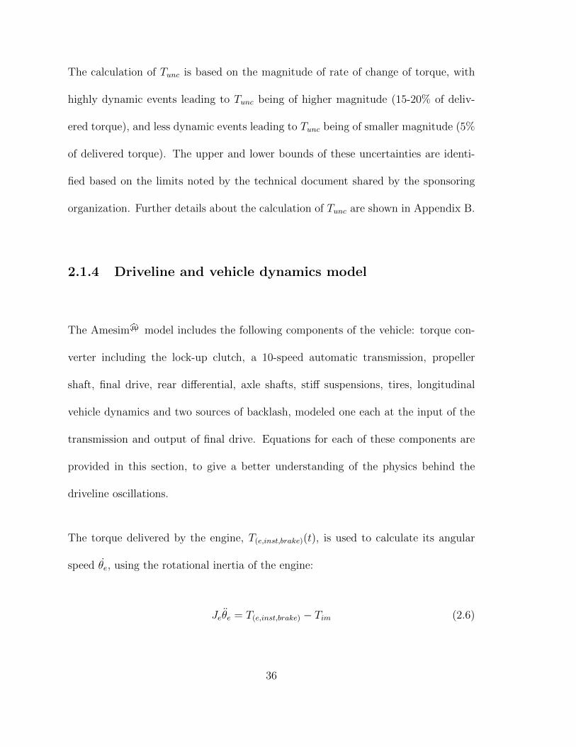
2.1.4 Driveline and vehicle dynamics model
The Amesim® model includes the following components of the vehicle: torque con-
verter including the lock-up clutch, a 10-speed automatic transmission, propeller
shaft, final drive, rear differential, axle shafts, stiff suspensions, tires, longitudinal
vehicle dynamics and two sources of backlash, modeled one each at the input of the
transmission and output of final drive. Equations for each of these components are
provided in this section, to give a better understanding of the physics behind the
driveline oscillations.
The torque delivered by the engine, T(e,inst,brake)(t), is used to calculate its angular
speed θe, using the rotational inertia of the engine:
Jeθe = T(e,inst,brake) − Tim (2.6)
36

where, Je is the rotational inertia of the engine, θe is the rotational acceleration of
the engine and Tim is the load torque at the impeller of the torque converter.
2.1.4.1 Torque converter model
The torque converter consists of an impeller, stator, turbine, and a lock-up clutch
with damper springs, set inside a metal housing. The lock-up clutch can operate
in one of its three modes when the vehicle is running: locked, open, or slipping.
In general, when the vehicle starts from a stationary state, the lock-up clutch is
open and complete torque transmission takes place through the fluid between the
impeller and turbine. When the vehicle reaches a set of pre-defined conditions (e.g.,
impeller speed, vehicle speed and transmission fluid temperature), the lock-up clutch
can operate in either slipping or locked positions. The transmission control unit
(TCU) defines the position of the lock-up clutch based on drivability target while
minimizing fuel consumption [39]. The modeled torque converter (Fig. 2.3) includes
both, the fluid path dynamics (due to the fluid inside the converter), and the lock-
up clutch dynamics. The fluid path dynamics are represented using look-up tables
which define the torque ratio and capacity factor of the converter based on its speed
ratio. The lock-up clutch dynamics are modeled based on its assumed clutch capacity.
Additionally, the hysteresis caused by the damper springs of the lock-up clutch inside
the torque converter are also modeled.
37

Figure 2.3: Amesim® model showing the torque converter with lock-upclutch and spring hysteresis blocks.
When the torque converter lock-up clutch operates in locked condition, it is assumed
that there are no losses in torque transmission, and that the impeller torque, Tim, is
completely transmitted to the torque converter turbine:
Ttu = Tim (2.7)
where, Ttu is the turbine torque of the torque converter.
The speed ratio (SR), torque ratio (TR) and capacity factor (K) of the torque con-
verter are defined as:
SR =θtu
θim(2.8)
38

where, θtu is the angular speed of the torque converter turbine and θim is the angular
speed of the torque converter impeller.
TR =TtuTim
(2.9)
K =θim(9.55)√
Tim(2.10)
where, θim is the angular speed of the torque converter impeller.
When the torque converter lock-up clutch operates in open condition, the turbine
torque, Ttu, is given by:
Ttu =
(θe(9.55)
K(SR)
)2
(TR(SR)) (2.11)
where, θe is the angular speed of the engine which is equal to the angular speed of
the torque converter impeller, K is the capacity factor of the torque converter as a
function of speed ratio SR, and TR is the torque ratio as a function of speed ratio
SR, of the torque converter.
When the torque converter lock-up clutch operates in slipping condition, the equation
39

is a combination of fluid path dynamics and clutch path dynamics and the turbine
torque, Ttu, is given by:
Ttu = Ttcc +
(θe(9.55)
K(SR)
)2
(TR(SR)) (2.12)
where Ttcc is the torque through the lock-up clutch.
It is important to note that the equations for the torque converter, discussed in this
work, are simplified equations and do not consider the effect of geometrical parameters
(like number of blades on the impeller and turbine, and their blade angles) and fluid
properties of the converter.
2.1.4.2 Automatic transmission model
Torque output from the torque converter flows through a 10-speed automatic trans-
mission whose schematic is shown in Fig. 2.4. It consists of 4 planetary gears and
6 clutch packs. Certain nodes for the transmission have been defined by the manu-
facturer, and inertias at these nodes were used for capturing its dynamics. A truth
table was defined in Amesim® which locks certain clutch packs, based on the gear
selected, leading to relevant torque multiplication.
40

Figure 2.4: Schematic diagram showing the 10-speed transmission[14].
The torque losses within the transmission (including transmission pump losses) have
been considered in the model, and are calculated based on engine speed, and gear
selected. These losses are subtracted from the torque converter output, and therefore,
the equation for torque flowing through the transmission, Ttr, is given by:
Ttr = (Ttu − Tgearloss)itr (2.13)
where, Tgearloss is the transmission torque loss, and itr is the gear ratio of the selected
gear.
41

Figure 2.5: Amesim® model showing the 10-speed automatic transmissionblocks.
42
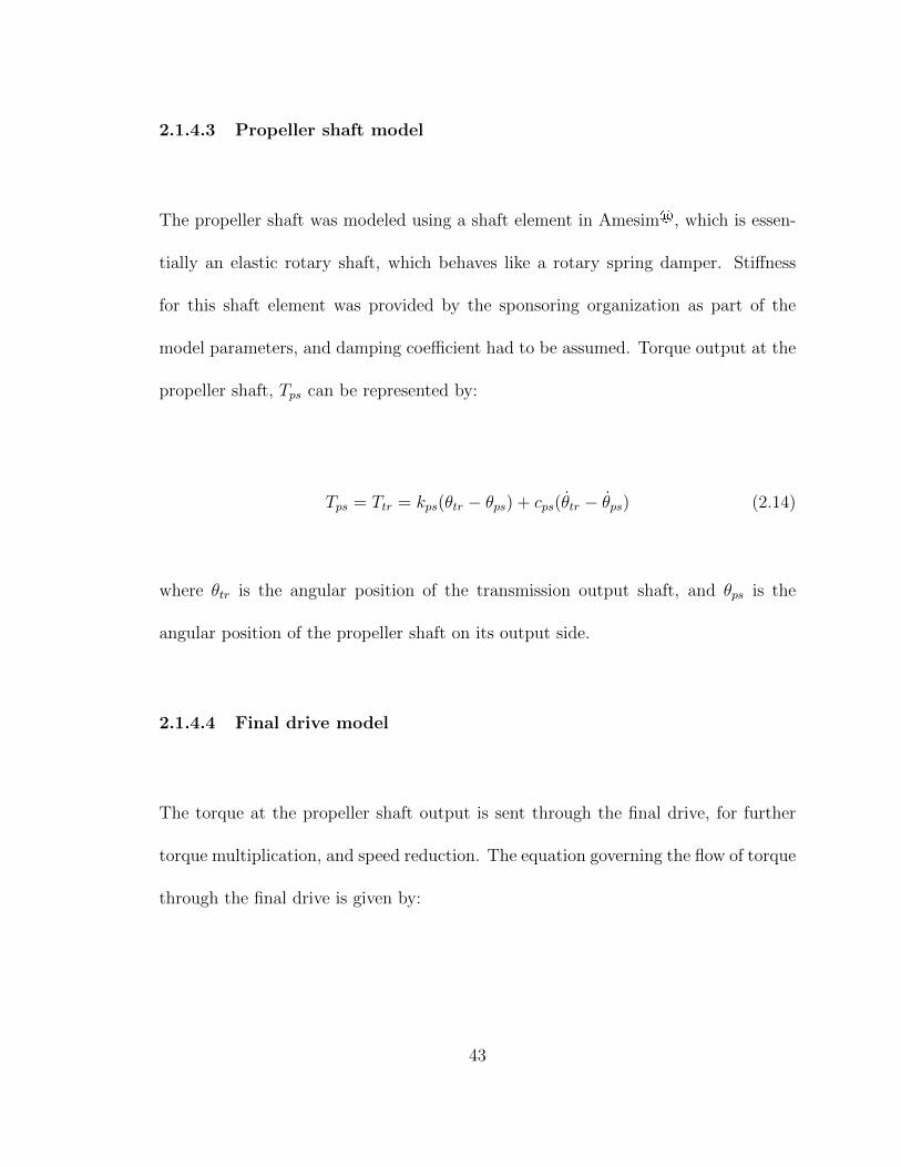
2.1.4.3 Propeller shaft model
The propeller shaft was modeled using a shaft element in Amesim®, which is essen-
tially an elastic rotary shaft, which behaves like a rotary spring damper. Stiffness
for this shaft element was provided by the sponsoring organization as part of the
model parameters, and damping coefficient had to be assumed. Torque output at the
propeller shaft, Tps can be represented by:
Tps = Ttr = kps(θtr − θps) + cps(θtr − θps) (2.14)
where θtr is the angular position of the transmission output shaft, and θps is the
angular position of the propeller shaft on its output side.
2.1.4.4 Final drive model
The torque at the propeller shaft output is sent through the final drive, for further
torque multiplication, and speed reduction. The equation governing the flow of torque
through the final drive is given by:
43

Tfd = Tpsifd (2.15)
where, Tfd is the torque output at the final drive, Tps is the torque output at the
propeller shaft, which is also the torque input to the final drive and ifd is the final
drive ratio.
2.1.4.5 Backlash model
Two rotary clearance blocks were placed in the Amesim® model for replicating
the backlashes, with the first one at the input of the transmission, representa-
tive of the transmission backlash and the second one at the output of the final
drive, representative of the final drive backlash. The rotary clearance block of the
Amesim® powertrain library was used for modeling the backlash because it takes
into account the clearance as well as impact at the face of gear teeth caused due to an
elastic end-stop, providing a more realistic picture of the expected output due to the
presence of backlash. Therefore, the stiffness and damping at the backlash element
can also be defined, if different, from the material of the shaft at which backlash is
modeled.
Backlash is representatively shown in Fig. 2.6. If 2α is considered to be the size of
backlash, then the possible positions of the backlash are −α for negative contact of
44
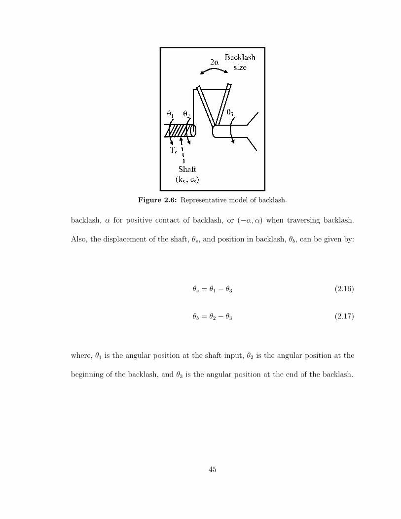
Figure 2.6: Representative model of backlash.
backlash, α for positive contact of backlash, or (−α, α) when traversing backlash.
Also, the displacement of the shaft, θs, and position in backlash, θb, can be given by:
θs = θ1 − θ3 (2.16)
θb = θ2 − θ3 (2.17)
where, θ1 is the angular position at the shaft input, θ2 is the angular position at the
beginning of the backlash, and θ3 is the angular position at the end of the backlash.
45

Figure 2.7: Amesim® model showing the propeller and axle shafts, alongwith the rear differential and final drive backlash.
Using equations 2.13 and 2.14, the backlash can be modeled as:
θb =
max{
0, θd + kscs
(θd − θb
)}, ifθb = −α
kscs
(θd − θb
)}, if |θb| < α
min{
0, θd + kscs
(θd − θb
)}, ifθb = +α
(2.18)
2.1.4.6 Axle shafts model
The rear differential, shown in Fig. 2.7, splits torque from the final drive such that it
is distributed between the two axle shafts. The axle shafts are modeled using a shaft
element in Amesim®, similar to the propeller shaft model. The torque, Tax flowing
through each axle shaft can be represented by:
46
Tax =Tfd2
= kax(θfd − θax) + cax(θfd − θax) (2.19)
where, kax, is the stiffness of the axle shaft, cax, is the damping coefficient of the axle
shaft, θfd, is the angular position of the final drive shaft, θax is the angular position
of the axle shaft at tire end, θfd, is the angular speed of the final drive shaft, and θax
is the angular speed of the axle shaft at tire end.
2.1.4.7 Suspension, tire and vehicle dynamics model
The suspension was modeled using a stiffness and damping element, that was con-
nected between the axle shafts and the tires. It was assumed stiff by providing a
large value to its stiffness and damping parameters in Amesim®. Using a detailed
suspension model was out of the scope of this work, and simplified parameters for its
stiffness and damping were not available during modeling.
The tires were modeled as a simplified stiffness and damping element along with
inertia. A Pacejka tire model [40], which is much more detailed that the stiffness and
damping element, was also developed as an alternative, but had to be discontinued
due to unavailability of some properties that were required by that model. The torque
at the tire, Tti, is given by:
47

Tti = Tax = kti(θax − θti) + cti(θax − θti) (2.20)
where, kti, is the stiffness of the tire, cti, is the damping coefficient of the tire, θax is
the angular position of the axle shaft, θti is the angular position of the tire, θax, is
the angular speed of the axle shaft, and θti, is the angular speed of the tire.
Longitudinal vehicle dynamics were modeled assuming 1D vehicle with two axles,
but with only the rear axle receiving propulsive torque. Aerodynamic force, rolling
resistance force, and slope force on the vehicle are considered through this block. The
equations for the longitudinal vehicle dynamics are modeled according to reference
[13], and are shown below:
Aerodynamic force:
Faero =1
2ρ Af CD (V )2 (2.21)
where, ρ is the air density, Af is the frontal area of the vehicle, CD is the drag
coefficient, V is the longitudinal velocity of the vehicle.
Rolling friction force:
Ffric = rveh V + Froll sign(V ) (2.22)
where, rveh is the coefficient of viscous friction, Froll is the rolling resistance force and
48

Figure 2.8: Amesim® model showing the suspension, tire and the vehicledynamics blocks.
V is the longitudinal velocity of the vehicle.
Froll = Rroll mveh g cos(δ) (2.23)
where Rroll is the rolling friction coefficient, mveh is the mass of the vehicle, g is the
gravitational acceleration, δ is the slope angle.
Slope force:
Fslope = mveh g sin(δ) (2.24)
The traction force generated by the engine, for propelling the vehicle can be given
49

by:
Ftraction =Ttirti
(2.25)
where, Tti, is the torque developed at the tire, and calculated in Eq. 2.20, and rti, is
the radius of the tire.
The acceleration of the vehicle is calculated according to the following formula:
aveh =Ftraction − Faero − Ffric − Fslope
mveh + Jwθw
(2.26)
where, the force components are calculated as per the previous equations, mveh is the
mass of the vehicle, Jw is the inertia of wheel hub, and θw is the angular speed of the
wheel hub, and is equal to the angular speed of the tire.
50

Figure 2.9: Overview of the Amesim® vehicle model.
51

2.2 Model validation
After developing the full-order vehicle model, experimental validation was carried
out to ensure that the model is able to capture the dynamics required for driveline
anti jerk controls work in the future. It is important to note that while most of the
required vehicle parameter data was provided by the sponsoring organization, there
were certain components whose detailed data could not be made available. One of
those was the torque converter, whose capacity factor, speed ratio, torque ratio curves
and inertia values were provided, but geometric properties like the number of blades
and blade angles of the impeller and turbine, and torque converter fluid properties
could not be made available. Therefore, the current model could only utilize a simple
look-up table based torque converter.
For validating the model, experimental tests were carried out by the sponsoring orga-
nization on a vehicle whose architecture was similar to the full-order model. The tests
involved multiple tip-in and tip-out sequences in three different modes of the torque
converter clutch (TCC). Also, the current production level control algorithms in place
for reducing the backlash induced oscillations on the test vehicle, were overridden
during the test. The experimental vehicle was instrumented with telemetric torque
sensors on the propeller shaft, seat-track accelerometers on the driver’s seat, and ac-
celerometers on the rear differential of the vehicle. The data from the accelerometers
52

Figure 2.10: Overview of the model validation work done.
53

has significant noise in it, which is visible in all the validation results’ plots. Also,
the entire range of CAN bus signals from various control units of the vehicle were
recorded, including base and instantaneous torque commands, estimated torque at
the crankshaft, engine speed, individual wheel speeds, and estimated torque in the
fluid path of the torque converter. These tests were carried out on a cold morning,
at a controlled test track.
Data collected from the vehicle can be classified based on the following conditions: a)
the torque converter clutch locked throughout the drive cycle, b) the torque converter
clutch unlocked or open throughout the drive cycle and c) the torque converter clutch
slipping during the tip-in events. While validating the simulation output, importance
was given to match parameters that would be of interest in controls related work, like
engine speed, wheel speed, vehicle acceleration and driveshaft torque. A step-by-step
approach, based on Newton’s second law of motion (F = ma), was taken to reduce
uncertainties in provided/assumed model parameters.
During validation, the case with TCC locked was used for fine-tuning the model
parameters in Amesim®. The final parameters after fine-tuning with the locked
TCC were used while validating scenarios with open and slipping TCC. An overview
of the model validation work is provided in Fig. 2.10.
54

2.2.1 Case 1: Torque converter lock-up clutch locked
In this case, the torque converter lock-up clutch through the TCU was explicitly
commanded to be in the locked position, for the entire drive cycle. Therefore, the
damping due to the fluid in the torque converter was negligible and consequently the
highest amplitude in driveline oscillations was observed in this case. For simulations,
the torque converter model was commanded a clutch capacity of 800 Nm, which
was well above the output from the engine. Therefore, the entire torque from the
engine passed through the lock-up clutch path. Based on the difference between the
simulation results and experimental results, model parameters were varied one after
another, in order to match the simulation results with the experimental results.
2.2.1.1 Sub-case 1: Original vehicle parameters
Initially, the simulation was run using the original vehicle parameters (Table 2.2),
provided by the sponsoring organization, for the modeled components. The torque
trajectory for the Amesim® model was calculated in Simulink®, using base and in-
stantaneous torque commands from the experimental data. The results obtained were
analyzed to interpret the changes that would be needed to the model. Fig. 2.11(a)
shows the estimated crankshaft torque calculated by the ECU, and the simulated
55

Table 2.1Frequency of driveline oscillations in sub-case 1
Jerk frequency fromtest vehicle
Jerk frequency fromsimulation
Error in jerkfrequency
5.88 Hz. 7.40 Hz. 25.85 %
crankshaft torque from the Simulink® model. Fig. 2.11(b),(c),(d) show the compar-
ison between the measured engine speed, vehicle speed, vehicle longitudinal acceler-
ation, propeller shaft torque, and respective simulated data.
The estimated and simulated crankshaft torques have a relatively small error dur-
ing the coasting period until 0.25 seconds. However, as soon as tip-in occurs, the
trajectories have significant variation, with the estimated crankshaft torque showing
more dynamic behavior compared to the simulated crankshaft torque. This issue is
addressed in the forthcoming sub-cases.
The vehicle speeds in Fig. 2.11 (b) show a close match, but the simulated engine speed
has considerable error when compared to the measured engine speed. In Fig. 2.11
(c), even though the measured seat-track acceleration is noisy, it is evident that the
simulated acceleration value is higher than the measured value. In Fig. 2.11 (d), there
is a phase delay between the measured and simulated propeller shaft torques during
transients, and a large mismatch during coasting condition.
The errors in engine speed and vehicle longitudinal acceleration were attributed to
56

0 0.25 0.5 0.75 1 1.25 1.5 1.75 2Time (s)
0T
1T
2T
3TC
ran
ksh
aft
torq
ue
(Nm
)
(a)
Estimated dataSimulated data
0 0.25 0.5 0.75 1 1.25 1.5 1.75 2Time (s)
12n
14n
16n
En
gin
esp
eed
(R
PM
)
40
50
60
70
80
Veh
icle
spee
d (
km/h
)
(b)
Measured engine dataSimulated engine data
Measured vehicle dataSimulated vehicle data
0 0.25 0.5 0.75 1 1.25 1.5 1.75 2Time (s)
-2a
0
2a
Veh
icle
lon
git
ud
inal
acce
lera
tio
n (
m/s
2)
(c)
Measured dataSimulated data
0 0.25 0.5 0.75 1 1.25 1.5 1.75 2Time (s)
0
0.4t
0.8t
Pro
pel
ler
shaf
tto
rqu
e (N
m)
(d)
Measured dataSimulated data
Figure 2.11: Results for sub-case 1 of model validation: Comparison be-tween experimental and simulation data with initial driveline parameters(Table 2.2).
57

Table 2.2Simulation parameters for Case 1
Parameter Value
Gear state 5TCC status LockedInput torque trajectory Calculated using engine modelMass of vehicle 2550 kgCoefficient of rolling resistance 0.02Propeller shaft stiffness Default valueAxle shaft stiffness Default valueEngine inertia Default valueTorque converter inertia Default valueTransmission inertia Default value
the mismatch in chosen value of vehicle mass for simulations, making the model
lighter than the actual vehicle, and causing the acceleration to be higher during
simulations. Therefore, the mass of the vehicle was recalculated based on inputs
from the manufacturer. Table 2.1 shows the difference in the frequencies of shuffle
oscillation measured on the vehicle, and in the simulation, for the tip-in scenario
shown. The error of 20.65 % in shuffle frequency points to a mismatch in the overall
inertia and the stiffness of the driveline model. This is addressed in the forthcoming
sub-cases.
58

Table 2.3Frequency of driveline oscillations in sub-case 2
Jerk frequency fromtest vehicle
Jerk frequency fromsimulation
Error in jerkfrequency
5.88 Hz. 7.40 Hz. 25.85 %
Table 2.4Simulation parameters for Case 2
Parameter Value
Gear state 5TCC status LockedInput torque trajectory Calculated using engine modelMass of vehicle 2884 kgCoefficient of rolling resistance 0.02Propeller shaft stiffness Default valueAxle shaft stiffness Default valueEngine inertia Default valueTorque converter inertia Default valueTransmission inertia Default value
2.2.1.2 Sub-case 2: Modified vehicle parameters - Vehicle mass increased
The vehicle mass was increased to account for the weight of the instruments used
during the tests, and of the three engineers who were present during the tests. The
parameters used for this simulation are provided in Table 2.4. The same tip-in sce-
nario as sub-case 1 was simulated again. Fig. 2.12 shows the result of this simulation.
59

0 0.25 0.5 0.75 1 1.25 1.5 1.75 2Time (s)
0T
1T
2T
3T
Cra
nks
haf
tto
rqu
e (N
m)
(a)
Estimated dataSimulated data
0 0.25 0.5 0.75 1 1.25 1.5 1.75 2Time (s)
12n
14n
16n
En
gin
esp
eed
(R
PM
)
40
50
60
70
80
Veh
icle
spee
d (
km/h
)
(b)
Measured engine dataSimulated engine data
Measured vehicle dataSimulated vehicle data
0 0.25 0.5 0.75 1 1.25 1.5 1.75 2Time (s)
-2a
0
2a
Veh
icle
lon
git
ud
inal
acce
lera
tio
n (
m/s
2)
(c)
Measured dataSimulated data
0 0.25 0.5 0.75 1 1.25 1.5 1.75 2Time (s)
0
0.4t
0.8t
Pro
pel
ler
shaf
tto
rqu
e (N
m)
(d)
Measured dataSimulated data
Figure 2.12: Results for sub-case 2 of model validation:Comparison between experimental and simulation data withincreased vehicle mass(Table 2.4).
60
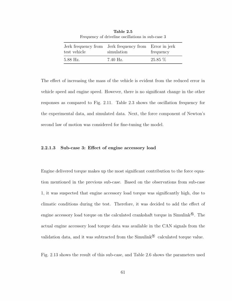
Table 2.5Frequency of driveline oscillations in sub-case 3
Jerk frequency fromtest vehicle
Jerk frequency fromsimulation
Error in jerkfrequency
5.88 Hz. 7.40 Hz. 25.85 %
The effect of increasing the mass of the vehicle is evident from the reduced error in
vehicle speed and engine speed. However, there is no significant change in the other
responses as compared to Fig. 2.11. Table 2.3 shows the oscillation frequency for
the experimental data, and simulated data. Next, the force component of Newton’s
second law of motion was considered for fine-tuning the model.
2.2.1.3 Sub-case 3: Effect of engine accessory load
Engine delivered torque makes up the most significant contribution to the force equa-
tion mentioned in the previous sub-case. Based on the observations from sub-case
1, it was suspected that engine accessory load torque was significantly high, due to
climatic conditions during the test. Therefore, it was decided to add the effect of
engine accessory load torque on the calculated crankshaft torque in Simulink®. The
actual engine accessory load torque data was available in the CAN signals from the
validation data, and it was subtracted from the Simulink® calculated torque value.
Fig. 2.13 shows the result of this sub-case, and Table 2.6 shows the parameters used
61

0 0.25 0.5 0.75 1 1.25 1.5 1.75 2Time (s)
0T
1T
2T
3T
Cra
nks
haf
tto
rqu
e (N
m)
(a)
Estimated dataSimulated data
0 0.25 0.5 0.75 1 1.25 1.5 1.75 2Time (s)
12n
14n
16n
En
gin
esp
eed
(R
PM
)
40
50
60
70
80
Veh
icle
spee
d (
km/h
)
(b)
Measured engine dataSimulated engine data
Measured vehicle dataSimulated vehicle data
0 0.25 0.5 0.75 1 1.25 1.5 1.75 2Time (s)
-2a
0
2a
Veh
icle
lon
git
ud
inal
acce
lera
tio
n (
m/s
2)
(c)
Measured dataSimulated data
0 0.25 0.5 0.75 1 1.25 1.5 1.75 2Time (s)
0
0.4t
0.8t
Pro
pel
ler
shaf
tto
rqu
e (N
m)
(d)
Measured dataSimulated data
Figure 2.13: Results for sub-case 3 of model validation: Comparison be-tween experimental and simulation data after increasing vehicle mass, andsubtracting engine accessory load torque (Table 2.6).
62

Table 2.6Simulation parameters for sub-case 3
Parameter Value
Gear state 5TCC status LockedInput torque trajectory Calculated using engine model
− Engine accessory load torqueMass of vehicle 2884 kgCoefficient of rolling resistance 0.02Propeller shaft stiffness Default valueAxle shaft stiffness Default valueEngine inertia Default valueTorque converter inertia Default valueTransmission inertia Default value
for simulation in this sub-case. The results show that the effect of engine accessory
load is not as significant as suspected, and the reduction in error between the signals
in subplots (b),(c) and (d), is negligible.
2.2.1.4 Sub-case 4: Using crankshaft torque signal from experimental
data
Another important difference between the experimental vehicle and the simulation
model was related to the engine. While the model utilizes a simplified natural aspi-
rated engine model for calculating the crankshaft torque, the test vehicle was equipped
with a turbocharged engine. The initial rise, followed by a lag and rise in the esti-
mated crankshaft torque, evident in subplot (a) of all the model validation plots,
63

Table 2.7Frequency of driveline oscillations in sub-case 4
Jerk frequency fromtest vehicle
Jerk frequency fromsimulation
Error in jerkfrequency
5.88 Hz. 7.40 Hz. 25.85 %
Table 2.8Simulation parameters for sub-case 4
Parameter Value
Gear state 5TCC status LockedInput torque trajectory Test vehicle crankshaft torqueMass of vehicle 2884 kgCoefficient of rolling resistance 0.02Propeller shaft stiffness Default valueAxle shaft stiffness Default valueEngine inertia Default valueTorque converter inertia Default valueTransmission inertia Default value
can be attributed to the dynamics of the turbocharger. Therefore, for the remaining
cases of validation, the estimated crankshaft torque was directly utilized as an input
to the Amesim® model. With this approach, the Amesim® model can be accurately
validated without having to worry about the dynamics of the turbocharger. Fig. 2.14
shows the response of this simulation.
The estimated crankshaft torque, and the simulated crankshaft torque in Fig. 2.14(a)
show a variation of 10% over the range of the simulation. This was deliberately
64

Figure 2.14: Results for sub-case 4 of model validation: Comparison be-tween experimental and simulation data with experimental crankshaft torquetrajectory as input.
65

included, based on the information provided by the sponsoring organization, about the
error in the estimated crankshaft torque. Modeling this error, provided some leeway,
to tune the input to the Amesim® model. In Fig. 2.14(b),(c),(d), the benefit of using
the estimated crankshaft torque is noticeable. The longitudinal vehicle acceleration,
propeller shaft torque, and vehicle speed show lower percentage of error compared
to sub-case 3. Therefore, it can be assumed that the force component developed by
the engine, has been reasonably fixed, by using estimated crankshaft torque as the
input to the Amesim® model. However, the simulated engine speed seems to be
less than the actual engine speed, which puts the focus on the resistive forces of the
longitudinal vehicle dynamics.
2.2.1.5 Sub-case 5: Modified coefficient of rolling resistance
As mentioned in the beginning of this section, the experimental tests were carried out
in a controlled test track, and therefore, any major perturbation in the slope force can
be ruled out. Similarly, the frontal area and the drag coefficient that were used for
calculating the aerodynamic force were based off calculations from a vehicle similar
to the test vehicle. However, there was a degree of uncertainty in the coefficient
used for calculating the rolling resistance force. Based on the fact that the coefficient
of rolling resistance for tires is dependent on a wide range of factors including the
construction of the tire, the speed with which the vehicle is traveling, the air pressure
66
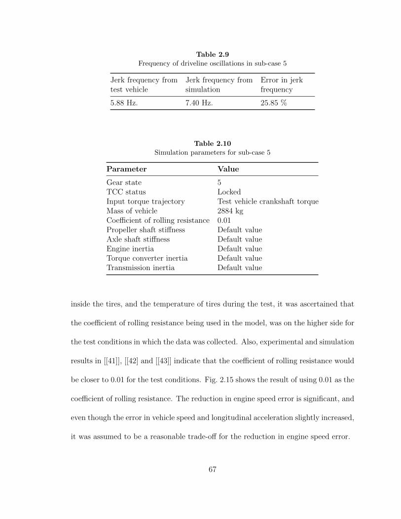
Table 2.9Frequency of driveline oscillations in sub-case 5
Jerk frequency fromtest vehicle
Jerk frequency fromsimulation
Error in jerkfrequency
5.88 Hz. 7.40 Hz. 25.85 %
Table 2.10Simulation parameters for sub-case 5
Parameter Value
Gear state 5TCC status LockedInput torque trajectory Test vehicle crankshaft torqueMass of vehicle 2884 kgCoefficient of rolling resistance 0.01Propeller shaft stiffness Default valueAxle shaft stiffness Default valueEngine inertia Default valueTorque converter inertia Default valueTransmission inertia Default value
inside the tires, and the temperature of tires during the test, it was ascertained that
the coefficient of rolling resistance being used in the model, was on the higher side for
the test conditions in which the data was collected. Also, experimental and simulation
results in [[41]], [[42] and [[43]] indicate that the coefficient of rolling resistance would
be closer to 0.01 for the test conditions. Fig. 2.15 shows the result of using 0.01 as the
coefficient of rolling resistance. The reduction in engine speed error is significant, and
even though the error in vehicle speed and longitudinal acceleration slightly increased,
it was assumed to be a reasonable trade-off for the reduction in engine speed error.
67

0 0.25 0.5 0.75 1 1.25 1.5 1.75 2Time (s)
0T
1T
2T
3T
Cra
nks
haf
tto
rqu
e (N
m)
(a)
Estimated dataSimulated data
0 0.25 0.5 0.75 1 1.25 1.5 1.75 2Time (s)
12n
14n
16n
En
gin
esp
eed
(R
PM
)
40
50
60
70
80
Veh
icle
spee
d (
km/h
)
(b)
Measured engine dataSimulated engine data
Measured vehicle dataSimulated vehicle data
0 0.25 0.5 0.75 1 1.25 1.5 1.75 2Time (s)
-2a
0
2a
Veh
icle
lon
git
ud
inal
acce
lera
tio
n (
m/s
2)
(c)
Measured dataSimulated data
0 0.25 0.5 0.75 1 1.25 1.5 1.75 2Time (s)
0
0.4t
0.8t
Pro
pel
ler
shaf
tto
rqu
e (N
m)
(d)
Measured dataSimulated data
Figure 2.15: Results for sub-case 5 of model validation:Comparison between experimental and simulation data withreduced coefficient of rolling resistance(Table 2.10.
68
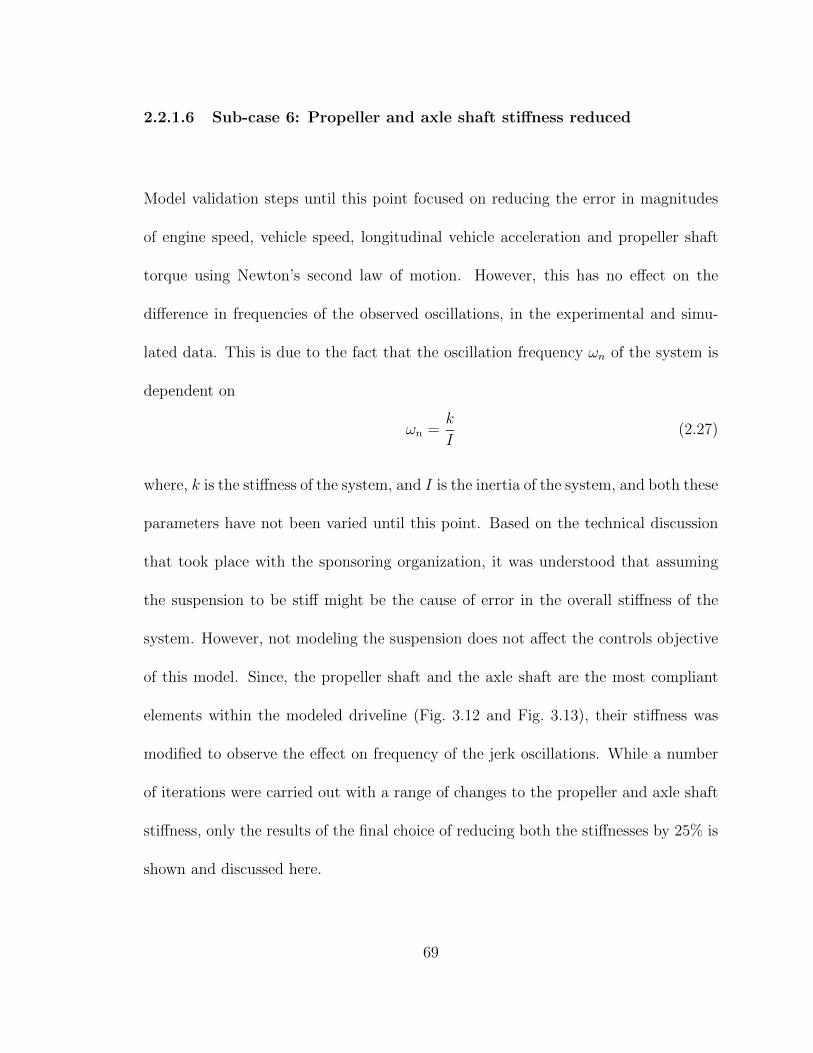
2.2.1.6 Sub-case 6: Propeller and axle shaft stiffness reduced
Model validation steps until this point focused on reducing the error in magnitudes
of engine speed, vehicle speed, longitudinal vehicle acceleration and propeller shaft
torque using Newton’s second law of motion. However, this has no effect on the
difference in frequencies of the observed oscillations, in the experimental and simu-
lated data. This is due to the fact that the oscillation frequency ωn of the system is
dependent on
ωn =k
I(2.27)
where, k is the stiffness of the system, and I is the inertia of the system, and both these
parameters have not been varied until this point. Based on the technical discussion
that took place with the sponsoring organization, it was understood that assuming
the suspension to be stiff might be the cause of error in the overall stiffness of the
system. However, not modeling the suspension does not affect the controls objective
of this model. Since, the propeller shaft and the axle shaft are the most compliant
elements within the modeled driveline (Fig. 3.12 and Fig. 3.13), their stiffness was
modified to observe the effect on frequency of the jerk oscillations. While a number
of iterations were carried out with a range of changes to the propeller and axle shaft
stiffness, only the results of the final choice of reducing both the stiffnesses by 25% is
shown and discussed here.
69

Table 2.11Frequency of driveline oscillations in sub-case 6
Jerk frequency fromtest vehicle
Jerk frequency fromsimulation
Error in jerkfrequency
5.88 Hz. 6.67 Hz. 13.43 %
The simulation parameters for sub-case 6 are shown in Table 2.12. Fig. 2.16 shows
the effect of reducing the propeller and axle shaft stiffness by 25%, in combination
with the changes that were made in the previous sub-cases. Compared to the result
of sub-case 5 (Fig. 2.15), there is a reduction in the error between the driveline
oscillation frequency of the test vehicle and the simulation, as shown in Table 2.11.
Since, frequency is also dependent on the inertia of the driveline elements (Eq. 2.27),
the next sub-case deals with increasing the inertia of certain driveline components to
match the oscillation frequency of jerk. This was exercised since there was a degree
of uncertainty in the overall inertia of the driveline, due to some components that
were not modeled. This is discussed in the next sub-case.
2.2.1.7 Sub-case 7: Engine, torque converter, and transmission inertia
adjusted
The vehicle architecture being modeled in this work, has a 4WD variant. The test
vehicle was a 4WD vehicle, whereas, the Amesim® model only considers a RWD
70
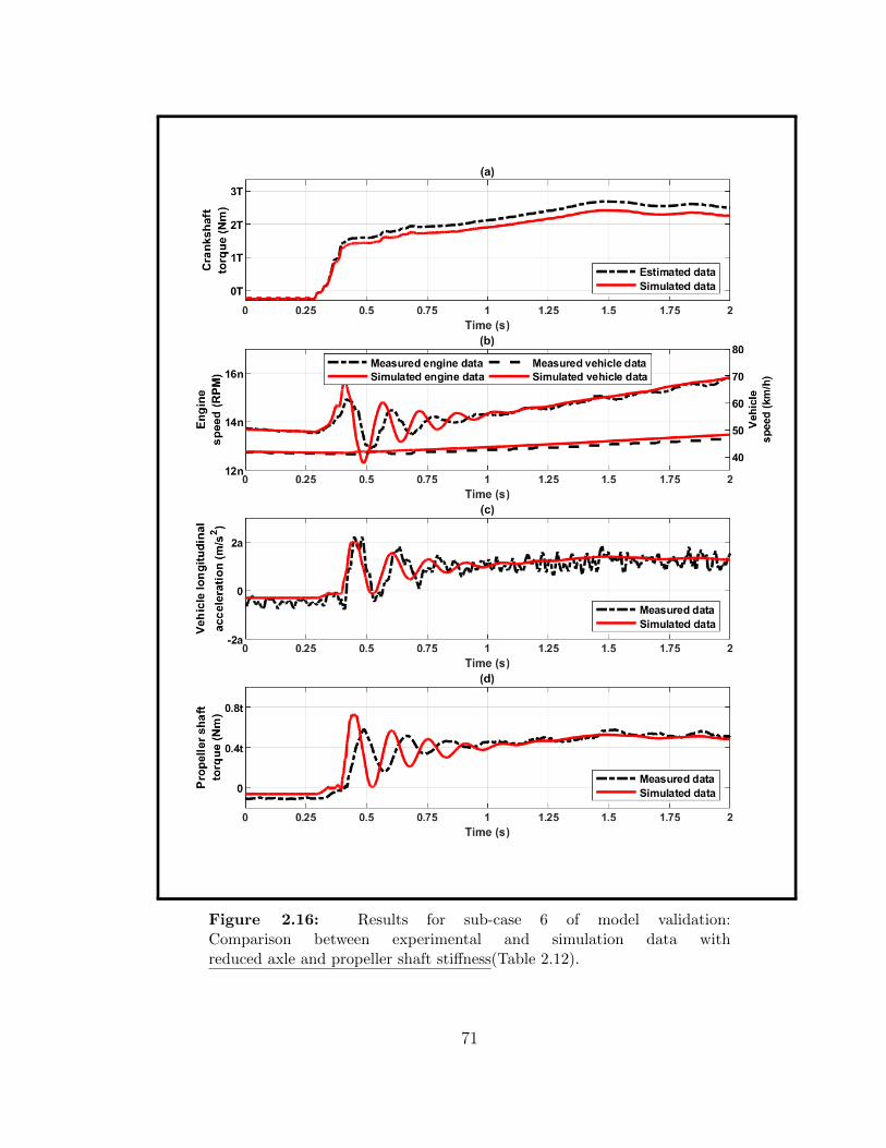
Figure 2.16: Results for sub-case 6 of model validation:Comparison between experimental and simulation data withreduced axle and propeller shaft stiffness(Table 2.12).
71

Table 2.12Simulation parameters for sub-case 6
Parameter Value
Gear state 5TCC status LockedInput torque trajectory Experimental crankshaft torqueMass of vehicle 2884 kgCoefficient of rolling resistance 0.01Propeller shaft stiffness Reduced by 25%Axle shaft stiffness Reduced by 25%Engine inertia Default valueTorque converter inertia Default valueTransmission inertia Default value
driveline. The transfer case present in a 4WD system, contributes significant inertia
at the end of the transmission, which is not captured in the Amesim® model. Also,
the crankshaft of the engine has a harmonic damper, which contributes significant
inertia to the overall driveline. These components could not be included in the model
as the sponsoring organization could not share this data. With this information, the
inertia of the engine, torque converter and one node of the transmission had to be
adjusted, in order to match the driveline jerk frequency observed on the test vehicle
with the simulation data.
The simulation parameters for sub-case 7 are shown in Table 2.14. Fig. 2.17 shows
the response of the driveline with 25% increase in the inertia of the engine, torque
converter, and final node of the transmission. The error in the frequency of the jerk
oscillation during tip-in, shown in Table 2.13, is negligible after these modifications.
72

Table 2.13Frequency of driveline oscillations in sub-case 7
Jerk frequency fromtest vehicle
Jerk frequency fromsimulation
Error in jerkfrequency
5.88 Hz. 5.84 Hz. 0.68 %
Table 2.14Simulation parameters for sub-case 7
Parameter Value
Gear state 5TCC status LockedInput torque trajectory Experimental crankshaft torqueMass of vehicle 2884 kgCoefficient of rolling resistance 0.01Propeller shaft stiffness Reduced by 25%Axle shaft stiffness Reduced by 25%Engine inertia Increased by 25%Torque converter inertia Increased by 25%Transmission inertia Increased by 25%
However, the propeller shaft torque still shows a phase difference between the mea-
sured and simulated data. This is addressed in sub-case 8.
2.2.1.8 Sub-case 8: Implementation of filter for propeller shaft torque
While validation results in the previous subsections show a phase difference between
the measured and simulated values of propeller shaft torque, it was mentioned by
73

Figure 2.17: Results for sub-case 7 of model validation:Comparison between experimental and simulation data withcrankshaft torque as input, reduced vehicle mass, reduced co-efficient of rolling resistance, reduced drive shaft stiffness, andincreased inertia of engine, torque converter and transmission(Table 2.14).
74

Table 2.15Filter parameters used for filtering simulated propeller shaft torque
Parameter Value
Response Type LowpassDesign Method IIR - Chebyshev IISampling frequency 1000 Hz.End frequency of passband 30 Hz.Beginning frequency of stopband 35 Hz.Passband ripple 1 dBStopband attenuation 120 dB
the sponsoring organization, that the telemetry device used for measuring the pro-
peller shaft torque output, had an in-built low pass filter with a cutoff frequency
of approximately 30 Hz. This contributed to the observed phase delay between the
measured and simulated torque values. To this end, a Chebyshev filter was designed
in MATLAB®, with the specifications listed in Table 2.15.
From Fig. 2.18(d), it is evident that there was, in fact, a filter with a cutoff frequency
of approximately 30 Hz., and implementing a filter on the simulated propeller shaft
torque data matches the phase of the measured and simulated data.
2.2.2 Case 2: Torque converter lock-up clutch open
As already mentioned in the model development section, the torque converter model
in this thesis, is based on a set of lookup tables for capacity factor, speed ratio, and
75

0 0.25 0.5 0.75 1 1.25 1.5 1.75 2Time (s)
0T
1T
2T
3T
Cra
nks
haf
tto
rqu
e (N
m)
(a)
Estimated dataSimulated data
0 0.25 0.5 0.75 1 1.25 1.5 1.75 2Time (s)
12n
14n
16n
En
gin
esp
eed
(R
PM
)
40
50
60
70
80
Veh
icle
spee
d (
km/h
)
(b)
Measured engine dataSimulated engine data
Measured vehicle dataSimulated vehicle data
0 0.25 0.5 0.75 1 1.25 1.5 1.75 2Time (s)
-2a
0
2a
Veh
icle
lon
git
ud
inal
acce
lera
tio
n (
m/s
2 ) (c)
Measured dataSimulated data
0 0.25 0.5 0.75 1 1.25 1.5 1.75 2Time (s)
0
0.4t
0.8t
Pro
pel
ler
shaf
tto
rqu
e (N
m)
(d)
Measured dataSimulated data
Figure 2.18: Simulation output in 5th gear with estimated crankshafttorque compensated for error as input to Amesim®, modified vehicle mass,modified coefficient of rolling resistance, modified propeller shaft and axleshaft stiffness, and modified engine, torque converter and transmission iner-tia, and filtered driveshaft torque.
76

torque ratio. These tables can be classified into two types, based on whether the
impeller is driving the turbine or the turbine is driving the impeller. The first case,
called normal run, takes place during normal driving scenarios, when the engine is
propelling the vehicle. The second case, called over run, takes place during coasting
scenarios, when the wheels propel the vehicle, and the speed of the turbine is higher
than the speed of the impeller. This causes the speed ratio of the torque converter to
exceed 1, and therefore, a separate lookup table of capacity factor is usually required
to accurately model its behavior. Lookup table data for the normal run case was
provided by the sponsoring organization, but data for the over-run case could not be
provided. Therefore, the over-run data had to be calculated based on information
provided in the Amesim® manual [13].
Simulation was performed after adjusting the model parameters, based on the ob-
servations from the locked TCC validation. Since the TCC is required to be open
throughout the run, the TCC capacity was set to 0 Nm, in the vehicle model.
Making use of calculated over-run lookup tables was good enough for the coasting
scenarios, as indicated in all the subplots of Fig. 2.19. However, using a simple steady
state torque converter model, based only on one- dimensional lookup tables, was not
enough to capture the transient dynamics of the tip-in scenario. Amesim® has pro-
vision to use a transient torque converter model, which is more detailed, but requires
geometric parameters like number of blades, blade angles, cross sectional area of flow
77

Table 2.16Simulation parameters for Case 2: TCC open condition
Parameter Value
Gear state 5TCC status OpenInput torque trajectory Experimental crankshaft torqueMass of vehicle 2884 kgCoefficient of rolling resistance 0.01Propeller shaft stiffness Reduced by 25%Axle shaft stiffness Reduced by 25%Engine inertia Increased by 25%Torque converter inertia Increased by 25%Transmission inertia Increased by 25%
passage, and fluid properties, like viscous friction coefficient, shock loss coefficient
etc. Since, these parameters were not available, the transient torque converter model
could not be used in Amesim®. At the end of this chapter, next steps that are being
taken to validate the model for transient torque converter events are discussed.
2.2.3 Case 3: Torque converter lock-up clutch slipping
In this case, the TCC is slipping during the tip-in scenarios, which means the flow
of torque in the torque converter is split between the fluid path and the lock-up
clutch path. The CAN signals from the experimental data contain an estimate of the
amount of torque flowing through the fluid path. This estimate was utilized to define
the lock-up clutch capacity in the Amesim® model, for this simulation.
78
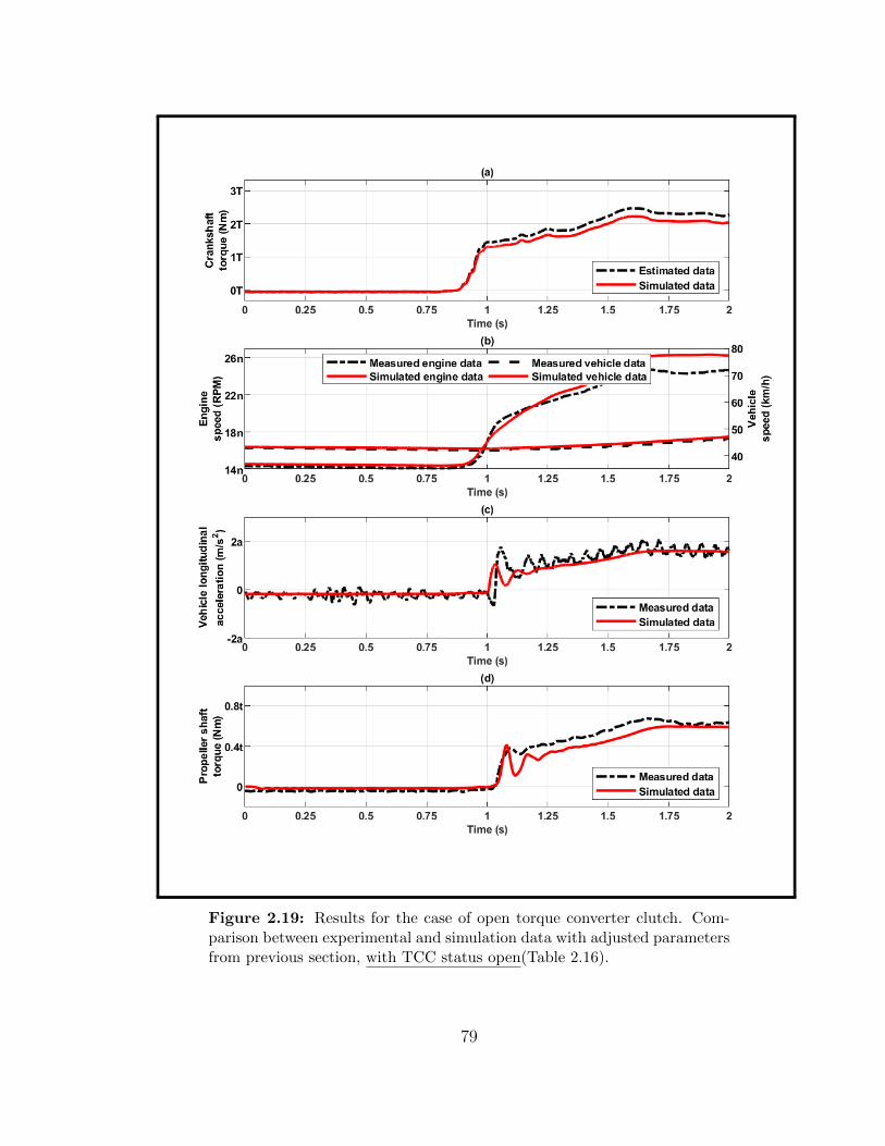
Figure 2.19: Results for the case of open torque converter clutch. Com-parison between experimental and simulation data with adjusted parametersfrom previous section, with TCC status open(Table 2.16).
79

Table 2.17Simulation parameters for Case 3: TCC slipping condition
Parameter Value
Gear state 5TCC status SlippingInput torque trajectory Experimental crankshaft torqueMass of vehicle 2884 kgCoefficient of rolling resistance 0.01Propeller shaft stiffness Reduced by 25%Axle shaft stiffness Reduced by 25%Engine inertia Increased by 25%Torque converter inertia Increased by 25%Transmission inertia Increased by 25%
Table 2.17 shows the simulation parameters for case 3, and Fig. 2.20 shows the re-
sponse of the driveline for this simulation. Similar to case 2, the torque converter
model used in Amesim® was able to provide a good match for the coasting scenarios,
but there is significant mismatch in the engine speed, vehicle longitudinal accelera-
tion, and propeller shaft torque during and after tip-in. This is again attributed to
the steady-state model of the torque converter that was used in Amesim®.
80

Figure 2.20: Results for the case of slipping torque converter clutch. Com-parison between experimental and simulation data, with adjusted parame-ters from previous section, and with TCC status slipping (Table 2.17).
81

Proposed solution to improve torque converter model:
It is clear from the results of Case 2, and Case 3 of model validation, that a steady
state torque converter model in Amesim® is ineffective in accurately capturing the
required transient dynamics of the fluid path torque. Since, the geometric and fluid
properties of the torque converter could not be made available, it was proposed that,
as a next step, required parametric data would be collected from a parallel hardware
project that is underway, on the same vehicle platform, at Michigan Technological
University. Then, an accurate model of the torque converter, for the vehicle in this
study, will be developed and integrated into the designed Amesim model in this thesis.
82

Chapter 3
Parametric Analysis of Driveline
Response
After model development and validation, parametric analysis of the model was per-
formed to understand the significance of various driveline elements, on shuffle oscil-
lations. Input torque ramp rate, transmission and final drive backlash size, propeller
and axle shaft stiffnesses and damping coefficients were of particular interest for para-
metric analysis. Each of these is discussed in this section and corresponding plots
are presented. This analysis was used to decide on the components to be considered
while reducing the model order.
83

3.1 Effect of varying input torque ramp rate
As mentioned in the first chapter, the magnitude of torque input and the time period
within which it is delivered, are major factors in defining the magnitude of oscillations
that are induced due to the backlash in the driveline. This was investigated for
various torque ramp rates from 150 Nm/s up to 1000 Nm/s. The results of two
of these ramp rates, i.e., 150 Nm/s and 500 Nm/s, are discussed in this section.
A ramp rate of 150 Nm/s represents a gradual torque request, and a ramp rate
of 500 Nm/s represents a sudden torque request by the driver. The engine speed,
vehicle longitudinal acceleration, transmission and final drive backlash traversal, and
propeller shaft torque were plotted to understand the response of the driveline.
3.1.1 Tip-in scenarios
Torque ramp rate can be commanded for both tip-in and tip-out scenarios in the
actual vehicle. Therefore, similar analysis was carried out, and this section presents
the results of the tip-in scenarios. The tip-in scenario can further be classified based
on the initial condition of backlash, and the status of the TCC. The initial condition
of backlash can either be positive contact or negative contact, and the status of TCC
can be (i) locked, (ii) slipping or (iii) open.
84

3.1.1.1 With backlash in positive contact and TCC locked
In this condition, the backlash is in positive contact, meaning the initial torque value
commanded to the engine was a positive value, and the final torque value commanded
is also positive. This case is analogous to a driver traveling on a highway with the
cruise control turned ON, and increasing the speed of the vehicle through the cruise
control system. Since the vehicle is at highway speeds, the TCC can be assumed to
be locked.
In Fig. 3.1, the base and instantaneous command torque rise from 50 Nm to 350 Nm
at a ramp rate of 150 Nm/s. The red line in Fig. 3.1 (a), is the delivered engine torque,
and it includes the first-order lag and, base and instantaneous path delays, which is
evident in its trajectory. Also, due to the included uncertainty in the engine model,
it is observed that there is an error of 10% between the commanded torque and the
delivered torque in steady state. Since the ramp rate is small, and the backlashes are
in positive contact, oscillations are not induced into the system, which is comparable
to an actual vehicle’s behavior under these conditions.
In Fig. 3.2, the base and instantaneous command torque rise from 50 Nm to 350 Nm
at a ramp rate of 500 Nm/s. Since, the torque uncertainty model uses a function
of ramp rate of the command signal for calculating the delivered torque, a drop in
engine delivered torque is observed at approximately 10.8 seconds. The increase in
85

9 9.5 10 10.5 11 11.5 12 12.5 13Time (s)
0
100
200
300
400
En
gin
eto
rqu
e (N
m)
0
500
1000
Clu
tch
cap
acit
y (N
m)
(a)
Base requested torqueInst. requested torqueEngine delivered torqueLock-up clutch capacity
9 9.5 10 10.5 11 11.5 12 12.5 13Time (s)
2200
2300
2400
En
gin
esp
eed
(R
PM
)
0
0.5
1
1.5
2
Veh
icle
lon
git
ud
inal
acce
lera
tio
n (
m/s
2 )
(b)
Engine speedVehicle acceleration
9 9.5 10 10.5 11 11.5 12 12.5 13Time (s)
-5
0
5
Bac
klas
hp
osi
tio
n (
deg
)
(c)
Transmission backlash positionFinal drive backlash position
9 9.5 10 10.5 11 11.5 12 12.5 13Time (s)
0
200
400
Pro
pel
ler
shaf
tto
rqu
e (N
m)
(d)
Propeller shaft torque
Figure 3.1: Driveline response for tip-in scenario with150 Nm/s ramp rate, backlash in positive contact, and locked TCC.
86

9 9.5 10 10.5 11 11.5 12 12.5 13Time (s)
0
100
200
300
400E
ng
ine
torq
ue
(Nm
)
0
500
1000
Clu
tch
cap
acit
y (N
m)
(a)
Base requested torqueInst. requested torqueEngine delivered torqueLock-up clutch capacity
9 9.5 10 10.5 11 11.5 12 12.5 13Time (s)
2000
2200
2400
En
gin
esp
eed
(R
PM
)
0
0.5
1
1.5
2
Veh
icle
lon
git
ud
inal
acce
lera
tio
n (
m/s
2 )
(b)
Engine speedVehicle acceleration
9 9.5 10 10.5 11 11.5 12 12.5 13Time (s)
-5
0
5
Bac
klas
hp
osi
tio
n (
deg
)
(c)
Transmission backlash positionFinal drive backlash position
9 9.5 10 10.5 11 11.5 12 12.5 13Time (s)
0
200
400
Pro
pel
ler
shaf
tto
rqu
e (N
m)
(d)
Propeller shaft torque
Figure 3.2: Driveline response for tip-in scenario with500 Nm/s ramp rate, backlash in positive contact, and locked TCC.
87

torque ramp rate leads to oscillations of small amplitude in the driveline, as evidenced
in the propeller shaft torque subplot (d) and, engine speed and vehicle acceleration
in subplot (b).
3.1.1.2 With backlash in negative contact and TCC locked
Next, the case wherein backlash is initially in negative contact is analyzed. The initial
torque command is in the negative domain, and it goes to positive domain when the
driver requests torque from the engine. Change in domain of delivered torque causes
the backlash to traverse from one side to the other. This case is analogous to a
vehicle which is coasting at highway speeds, with the driver’s foot off the accelerator
pedal and the cruise control turned OFF, causing the vehicle’s momentum to propel
the vehicle. Then, the driver requests torque either through the accelerator pedal or
through the cruise control, and the engine starts delivering torque to the driveline.
In Fig. 3.3, the base and instantaneous command torque rise from 50 Nm to 350 Nm
at a ramp rate of 150 Nm/s, from negative contact of backlash to positive contact.
Since the engine is providing torque, the backlash at the transmission traverses first,
and as soon as it reaches positive contact, the backlash at the final drive traverses.
Both these backlash elements cause an impact on making positive contact, and induce
oscillations throughout the driveline, as evidenced in propeller shaft torque and vehicle
acceleration in subplots Fig. 3.3(b) and (d) . Oscillations of the same frequency are
88

observed in the engine speed θe, which is being calculated in Amesim, using the
formula:
Jeθe = T(e,inst,brake)(t)− Tim (3.1)
wherein, Je is the rotational inertia of the engine, θe is the rotational acceleration of
the engine, from which rotational speed is computed and Tim is the load torque from
the driveline, at the impeller of the torque converter. The load torque carries over
the shuffle oscillations observed in the propeller shaft torque.
A similar tip-in scenario is shown in Fig. 3.4, with the the backlash in negative
contact, and the TCC in locked position. However, the ramp rate of the input torque
in this case is 500 Nm/s, which causes the backlash traversal to take place quicker
than the previous case. This leads to an increased impact velocity at positive contact
of the transmission and final drive backlash, causing the amplitude of the induced
oscillations to be higher than the case where the input torque ramp rate is 150 Nm/s.
The frequency of the oscillation, however, does not change, as it is related to the
stiffness of the components of the driveline, rather than the input given to the system.
89

9 10 11 12 13 14 15Time (s)
0
100
200
En
gin
eto
rqu
e (N
m)
0
500
1000
Clu
tch
cap
acit
y (N
m)
(a)
Base requested torqueInst. requested torqueEngine delivered torqueLock-up clutch capacity
9 10 11 12 13 14 15Time (s)
1500
1600
1700
1800
1900
2000
En
gin
esp
eed
(R
PM
)
-0.5
0
0.5
1
Veh
icle
lon
git
ud
inal
acce
lera
tio
n (
m/s
2 )
(b)
Engine speedVehicle acceleration
9 10 11 12 13 14 15Time (s)
-5
0
5
Bac
klas
hp
osi
tio
n (
deg
)
(c)
Transmission backlash positionFinal drive backlash position
9 10 11 12 13 14 15Time (s)
0
100
200
300
400
Pro
pel
ler
shaf
tto
rqu
e (N
m)
(d)
Propeller shaft torque
Figure 3.3: Driveline response for tip-in scenario with 150 Nm/s ramp rate,backlash in negative contact, and locked TCC.
90

9 10 11 12 13 14 15Time (s)
0
100
200E
ng
ine
torq
ue
(Nm
)
0
500
1000
Clu
tch
cap
acit
y (N
m)
(a)
Base requested torqueInst. requested torqueEngine delivered torqueLock-up clutch capacity
9 10 11 12 13 14 15Time (s)
1600
1800
2000
En
gin
esp
eed
(R
PM
)
-0.5
0
0.5
1
Veh
icle
lon
git
ud
inal
acce
lera
tio
n (
m/s
2 )
(b)
Engine speedVehicle acceleration
9 10 11 12 13 14 15Time (s)
-5
0
5
Bac
klas
hp
osi
tio
n (
deg
)
(c)
Transmission backlash positionFinal drive backlash position
9 10 11 12 13 14 15Time (s)
0
100
200
300
400
Pro
pel
ler
shaf
tto
rqu
e (N
m)
(d)
Propeller shaft torque
Figure 3.4: Driveline response for tip-in scenario with 500 Nm/s ramp rate,backlash in negative contact, and locked TCC.
91

3.1.1.3 With backlash in negative contact and TCC slipping
The fluid path of the torque converter is capable of damping out the oscillations
induced into the driveline due to backlash traversal. In fact, this property can be
utilized as a means of mitigating the jerk in the driveline. This was tested by reducing
the clutch capacity of the system from 800 Nm (Locked case), to 100 Nm (Slipping
case), and providing a base and instantaneous torque command at a ramp rate of
500 Nm/s. Fig. 3.5 shows the response of the driveline for this scenario. The torque
converter lock up clutch is in the locked position until a torque value of 100 Nm
from the engine, and above that it starts to slip, meaning the flow of torque in the
torque converter model is distributed between the fluid path and the lock-up clutch
path. Both the propeller shaft torque and the vehicle longitudinal acceleration show
reduced oscillations compared to the case where the torque converter lock up clutch
was locked. In an actual vehicle, the pressure command to the torque converter lock
up clutch can be varied during backlash traversal, such that the jerk in the driveline
is further reduced.
92

9 10 11 12 13 14 15Time (s)
0
100
200
En
gin
eto
rqu
e (N
m)
0
500
1000
Clu
tch
cap
acit
y (N
m)
(a)
Base requested torqueInst. requested torqueEngine delivered torqueLock-up clutch capacity
9 10 11 12 13 14 15Time (s)
1500
2000
2500
En
gin
esp
eed
(R
PM
)
-0.5
0
0.5
1
Veh
icle
lon
git
ud
inal
acce
lera
tio
n (
m/s
2 )
(b)
Engine speedVehicle acceleration
9 10 11 12 13 14 15Time (s)
-5
0
5
Bac
klas
hp
osi
tio
n (
deg
)
(c)
Transmission backlash positionFinal drive backlash position
9 10 11 12 13 14 15Time (s)
0
100
200
300
400
Pro
pel
ler
shaf
tto
rqu
e (N
m)
(d)
Propeller shaft torque
Figure 3.5: Driveline response for tip-in scenario with 500 Nm/s ramp rate,backlash in negative contact, and slipping TCC.
93

3.1.2 Tip-out scenarios
It is possible to experience clunk and shuffle even during tip-out scenarios, and there-
fore requires a separate set of algorithms for managing backlash traversal when the
driver lifts his/her foot off the accelerator pedal, or the cruise control stops requesting
torque from the engine. It is necessary to understand the behavior of the driveline
during such scenarios, to aid the development of the required control strategy.
While it has already been established in the subsection 3.1.1, that unlocking the TCC
during backlash traversal is beneficial for reducing jerk, it is not always recommended
from a fuel economy point of view. Therefore, tip-out scenarios were also sub-classified
into cases when the TCC is locked, and when it is slipping or open, to understand
the effect each of these cases has on the driveline response.
3.1.2.1 With backlash in positive contact and TCC locked
In Fig. 3.6, the base and instantaneous torque command fall from 350 Nm to 50 Nm
at a ramp rate of 150 Nm/s, with the backlash in positive contact, and the TCC
in locked position. Since the torque command is in the positive domain throughout
the scenario, backlash traversal does not take place, and therefore, the response of
the driveline is smooth, and similar to the tip-in case with locked TCC and positive
94

contact of backlash.
3.1.2.2 With backlash in negative contact and TCC locked
In Fig. 3.7, the base and instantaneous command torque fall from 250 Nm to -50 Nm
at a ramp rate of 150 Nm/s, from positive contact of backlash to negative contact,
with the TCC locked. In this case, the final drive backlash traverses first, and as
soon as it makes negative contact, transmission backlash traversal takes place. This
causes clunk and shuffle in the system, just as in the case of tip-in scenarios. Since,
the backlash traversal takes place after the delivered engine torque changes domain,
it is only required to control the engine delivered torque as it reaches a value close to
0 Nm.
3.1.2.3 With backlash in negative contact and TCC open
In Fig. 3.8, the base and instantaneous command torque fall from 250 Nm to -50 Nm
at a ramp rate of 150 Nm/s, from positive contact of backlash to negative contact,
with the TCC capacity set to 0 Nm. Therefore, the TCC remains open throughout the
scenario, and the entire torque flows through the fluid path of the torque converter.
Just as in the case of tip-in scenario with slipping lock up clutch inside the torque
converter, having an open lock up clutch during tip-out scenario also reduces jerk in
95

9 10 11 12 13 14 15Time (s)
0
100
200
300
400
En
gin
eto
rqu
e (N
m)
799
799.5
800
800.5
801
Clu
tch
cap
acit
y (N
m)
(a)
Base requested torqueInst. requested torqueEngine delivered torqueLock-up clutch capacity
9 10 11 12 13 14 15Time (s)
2800
2900
3000
3100
3200
En
gin
esp
eed
(R
PM
)
0
0.5
1
1.5
2
Veh
icle
lon
git
ud
inal
acce
lera
tio
n (
m/s
2 )
(b)
Engine speedVehicle acceleration
9 10 11 12 13 14 15Time (s)
-5
0
5
Bac
klas
hp
osi
tio
n (
deg
)
(c)
Transmission backlash positionFinal drive backlash position
9 10 11 12 13 14 15Time (s)
0
200
400
Pro
pel
ler
shaf
tto
rqu
e (N
m)
(d)
Propeller shaft torque
Figure 3.6: Driveline response for tip-out scenario with 150 Nm/s ramprate, backlash in positive contact, and locked TCC.
96
9 10 11 12 13 14 15Time (s)
0
100
200
En
gin
eto
rqu
e (N
m)
799
799.5
800
800.5
801
Clu
tch
cap
acit
y (N
m)
(a)
Base requested torqueInst. requested torqueEngine delivered torqueLock-up clutch capacity
9 10 11 12 13 14 15Time (s)
2600
2650
2700
2750
2800
En
gin
esp
eed
(R
PM
)
-2
-1
0
1
2
Veh
icle
lon
git
ud
inal
acce
lera
tio
n (
m/s
2 )
(b)
Engine speedVehicle acceleration
9 10 11 12 13 14 15Time (s)
-5
0
5
Bac
klas
hp
osi
tio
n (
deg
)
(c)
Transmission backlash positionFinal drive backlash position
9 10 11 12 13 14 15Time (s)
-200
0
200
400
Pro
pel
ler
shaf
tto
rqu
e (N
m)
(d)
Propeller shaft torque
Figure 3.7: Driveline response for tip-out scenario with 150 Nm/s ramprate, backlash in negative contact, and locked TCC.
97
the system.
3.1.3 During backlash traversal
From the previous analyses in this chapter, it is evident that controlling the speed
with which backlash traversal takes place, is essential for reducing clunk and shuffle
in the driveline. Therefore, varying the torque ramp rate is carried out in such a way,
that the impact velocity on the positive contact of backlash is reduced.
In Fig. 3.9, the base torque command rises from -50 Nm to 250 Nm at a ramp rate of
500 Nm/s, while the instantaneous torque command first rises at the same ramp rate,
and then suddenly drops during backlash traversal, and then rises again to merge with
the base torque command. The TCC is locked in this condition, and therefore, there
is no damping from the fluid path of the torque converter. Compared to Fig. 3.4, the
amplitude of oscillation in vehicle longitudinal acceleration is reduced by nearly 50 %,
and in propeller shaft torque it is reduced by nearly 30 %. As the instantaneous path
torque command controls the spark during combustion, it is capable of handling such
quick dynamics. However, the effect of drop in instantaneous path torque command,
on other parameters like fuel economy has to be studied.
98

9 10 11 12 13 14 15Time (s)
0
100
200
En
gin
eto
rqu
e (N
m)
0
500
1000
Clu
tch
cap
acit
y (N
m)
(a)
Base requested torqueInst. requested torqueEngine delivered torqueLock-up clutch capacity
9 10 11 12 13 14 15Time (s)
2600
2800
3000
En
gin
esp
eed
(R
PM
)
-1
0
1
Veh
icle
lon
git
ud
inal
acce
lera
tio
n (
m/s
2)(b)
Engine speedVehicle acceleration
9 10 11 12 13 14 15Time (s)
-5
0
5
Bac
klas
hp
osi
tio
n (
deg
)
(c)
Transmission backlash positionFinal drive backlash position
9 10 11 12 13 14 15Time (s)
0
200
400
Pro
pel
ler
shaf
tto
rqu
e (N
m)
(d)
Propeller shaft torque
Figure 3.8: Driveline response for tip-out scenario with 150 Nm/s ramprate, backlash in negative contact, and open TCC.
99

9 9.5 10 10.5 11 11.5 12 12.5 13Time (s)
0
100
200
En
gin
eto
rqu
e (N
m)
0
500
1000
Clu
tch
cap
acit
y (N
m)
(a)
Base requested torqueInst. requested torqueEngine delivered torqueLock-up clutch capacity
9 9.5 10 10.5 11 11.5 12 12.5 13Time (s)
1600
1700
1800
En
gin
esp
eed
(R
PM
)
-0.5
0
0.5
1
Veh
icle
lon
git
ud
inal
acce
lera
tio
n (
m/s
2 )
(b)
Engine speedVehicle acceleration
9 9.5 10 10.5 11 11.5 12 12.5 13Time (s)
-5
0
5
Bac
klas
hp
osi
tio
n (
deg
)
(c)
Transmission backlash positionFinal drive backlash position
9 9.5 10 10.5 11 11.5 12 12.5 13Time (s)
0
100
200
300
400
Pro
pel
ler
shaf
tto
rqu
e (N
m)
(d)
Propeller shaft torque
Figure 3.9: Driveline response for tip-in scenario with torque ramp ratevarying during backlash traversal. The backlash is initially in negative con-tact, and TCC is locked.
100
3.2 Effect of varying backlash size
3.2.1 Variation in transmission backlash
In an automobile, the size of the backlash is dependent on factors such as the con-
struction of the gear element, the wear and tear in the components, etc. Also, the
transmission may have different backlash sizes for different gear states. Therefore, it
is necessary to understand the effect of variation in backlash size of both the trans-
mission backlash, and the final drive backlash. This would give an idea as to where
the lumped backlash element in the reduced-order model (ROM) should be placed.
Transmission backlash varies from gear state to gear state, because of the construc-
tion of the gear train in the transmission assembly. The effect of variation in the
transmission backlash is comparatively analyzed in Fig. 3.10. A torque input of 500
Nm/s is provided, and the commanded torque goes from -50 Nm to 250 Nm. The
backlash is in negative contact initially, and the TCC is locked throughout the sim-
ulation. In case A, the transmission backlash size was 10 deg., and in case B, the
transmission backlash size was increased to 20 deg. Having a larger backlash size
naturally increases the response time of the system, but the difference for these cases
is nominal. There is an increase of 8 % in the oscillation amplitude of propeller shaft
101

torque in Case B, as compared to Case A, and an increase of 9.8 % in the oscillation
amplitude of vehicle longitudinal acceleration in Case B, as compared to Case A. This
increase can be attributed to the increased travel that the transmission backlash in
case B has to traverse, giving it a higher impact velocity.
3.2.2 Variation in final drive backlash
The final drive backlash can vary due to wear and tear of the components, leading
to a gradual increase in its size. The effect of variation in the final drive backlash is
comparitively analyzed in Fig. 3.11. The simulation conditions were same as in the
case of varying the transmission backlash size. The final drive backlash size was 4 deg.
in case A, and 8 deg. in case B. From the results in Fig. 3.11, it is clear that an increase
in the final drive backlash size makes the response of the system singificantly slower
compared to an increase in transmission backlash. Also, the amplitude of oscillations
of vehicle acceleration increased by an average of 37 % in Case B, compared to Case
A. This can be attributed to the fact that the torque flowing through the final drive
backlash is higher than the torque flowing through the transmission backlash, as
torque multiplication takes place within the system, leading to larger amplitude of
oscillation. Also, the rotational speed at the final drive backlash is comparatively
less than the speed at the transmission backlash, which explains the delay in system
response.
102

9.5 10 10.5 11 11.5Time (s)
0
100
200E
ng
ine
torq
ue
(Nm
)
0
500
1000
Clu
tch
cap
acit
y (N
m)
(a)
Base requested torqueInst. requested torqueEngine delivered torqueLock-up clutch capacity
9.5 10 10.5 11 11.5Time (s)
1800
2000
2200
2400
2600
En
gin
esp
eed
(R
PM
)
-0.5
0
0.5
1
Veh
icle
lon
git
ud
inal
acce
lera
tio
n (
m/s
2 )(b)
Engine speed (Case A)Engine speed (Case B)Vehicle accln (Case A)Vehicle accln (Case B)
9.5 10 10.5 11 11.5Time (s)
-10
-5
0
5
10
Bac
klas
hp
osi
tio
n (
deg
)
(c)
Transmission backlash position (Case A)Transmission backlash position (Case B)Final drive backlash position (Case A)Final drive backlash position (Case B)
9.5 10 10.5 11 11.5Time (s)
0
200
400
Pro
pel
ler
shaf
tto
rqu
e (N
m)
(d)
Propeller shaft torque (Case A)Propeller shaft torque (Case B)
Figure 3.10: Effect of changing the transmission backlash on drivelineresponse. Case A represents condition where transmission backlash is 10deg. Case B represents condition where transmission backlash is 20 deg.
103

9.5 10 10.5 11 11.5Time (s)
0
100
200
En
gin
eto
rqu
e (N
m)
0
500
1000
Clu
tch
cap
acit
y (N
m)
(a)
Base requested torqueInst. requested torqueEngine delivered torqueLock-up clutch capacity
9.5 10 10.5 11 11.5Time (s)
1800
2000
2200
2400
2600
En
gin
esp
eed
(R
PM
)
-0.5
0
0.5
1
Veh
icle
lon
git
ud
inal
acce
lera
tio
n (
m/s
2 )(b)
Engine speed (Case A)Engine speed (Case B)Vehicle accln (Case A)Vehicle accln (Case B)
9.5 10 10.5 11 11.5Time (s)
-10
-5
0
5
10
Bac
klas
hp
osi
tio
n (
deg
)
(c)
Transmission backlash position (Case A)Transmission backlash position (Case B)Final drive backlash position (Case A)Final drive backlash position (Case B)
9.5 10 10.5 11 11.5Time (s)
0
200
400
Pro
pel
ler
shaf
tto
rqu
e (N
m)
(d)
Propeller shaft torque (Case A)Propeller shaft torque (Case B)
Figure 3.11: Effect of increasing the final drive backlash on driveline re-sponse. Case A represents condition where final drive backlash is 4 deg.Case B represents condition where final drive backlash is 8 deg.
104

3.3 Effect of varying propeller and axle shaft prop-
erties
In a rear wheel driven vehicle powertrain, the propeller shaft and axle shafts are prone
to the highest elastic deformations, making them the most compliant elements of the
driveline. Therefore, the effect of changing the individual properties of these shafts,
on the response of the vehicle driveline was studied. Though it is known that a change
in stiffness of the shaft would bring about a change in the damping coefficient of the
shaft, it was assumed in these analyses that they can be individually modified. The
results of this analysis was used to determine the location of the lumped stiffness and
damping coefficient elements in the ROM.
3.3.1 Effect of varying propeller shaft stiffness
The natural frequency of a system is based on its stiffness and mass (or inertia in this
case). Since the inertia of the propeller shaft is low compared to the other inertial
elements in the driveline, the stiffness of the propeller shaft was varied to analyze its
impact on the response of the driveline, and a comparitive result of this analysis is
shown in Fig. 3.12. An input torque is commanded from -50 Nm to 250 Nm, at a ramp
rate of 500 Nm/s, the backlash is initially in negative contact, and the TCC is locked.
105

In case A, the propeller shaft stiffness is decreased by 25% from its final modified
value in Chapter 2, and in case B, it is increased by 25%. Since, the frequency is
directly proportional to the stiffness, it was observed that increasing the stiffness of
the propeller shaft, increased the frequency of oscillations, and vice versa. In case A,
the oscillation frequency in propeller shaft torque decreased by 1.97%, and in case B,
the oscillation frequency is increased by 1.43%. It was also observed that changing
the stiffness, does not have an effect on the amplitude of oscillations.
3.3.2 Effect of varying axle shaft stiffness
Similar analysis was carried out on the axle shaft, by increasing and decreasing its
stiffness by 25% of the final value considered for model validation in Chapter 2. The
input conditions for the simulations were similar to the previous case of propeller
shaft stiffness analysis. The results of this analysis are shown in Fig. 3.13. The
driveline response was similar as in the case of modified propeller shaft stiffness, but
it was observed that the change in frequency of oscillations, with a change in axle
shaft stiffness, was higher. In case A, for a decrease in axle shaft stiffness by 25%,
a decrease in oscillation frequency of propeller shaft torque by 4.49% was observed.
In case B, for an increase in axle shaft stiffness by 25%, an increase in oscillation
frequency of propeller shaft torque by 3.95% was observed. This can be attributed
to the increased magnitude of torque flowing through the axle shafts, compared to
106

9.5 10 10.5 11 11.5Time (s)
0
100
200E
ng
ine
torq
ue
(Nm
)
0
200
400
600
800
1000
Clu
tch
cap
acit
y (N
m)
(a)
Base requested torqueInst. requested torqueEngine delivered torqueLock-up clutch capacity
9.5 10 10.5 11 11.5Time (s)
1800
2000
2200
2400
2600
En
gin
esp
eed
(R
PM
)
-0.5
0
0.5
1
Veh
icle
lon
git
ud
inal
acce
lera
tio
n (
m/s
2 )
(b)
Engine speed (Case A)Engine speed (Case B)Vehicle accln (Case A)Vehicle accln (Case B)
9.5 10 10.5 11 11.5Time (s)
-10
-5
0
5
10
Bac
klas
hp
osi
tio
n (
deg
)
(c)
Transmission backlash position (Case A)Transmission backlash position (Case B)Final drive backlash position (Case A)Final drive backlash position (Case B)
9.5 10 10.5 11 11.5Time (s)
-100
0
100
200
300
400
Pro
pel
ler
shaf
tto
rqu
e (N
m)
(d)
Propeller shaft torque (Case A)Propeller shaft torque (Case B)
Figure 3.12: Effect of changing propeller shaft stiffness on overall drivelineresponse. Case A represents condition where propeller shaft stiffness is de-creased by 25%. Case B represents condition where propeller shaft stiffnessis increased by 25%.
107

the propeller shaft. Even though the axle shafts are stiffer than the propeller shaft,
the ratio of difference in torques flowing through them is higher than the ratio of
difference in stiffness.
108

9.5 10 10.5 11 11.5Time (s)
0
100
200E
ng
ine
torq
ue
(Nm
)
0
200
400
600
800
1000
Clu
tch
cap
acit
y (N
m)
(a)
Base requested torqueInst. requested torqueEngine delivered torqueLock-up clutch capacity
9.5 10 10.5 11 11.5Time (s)
1800
2000
2200
2400
2600
En
gin
esp
eed
(R
PM
)
-0.5
0
0.5
1
Veh
icle
lon
git
ud
inal
acce
lera
tio
n (
m/s
2 )
(b)
Engine speed (Case A)Engine speed (Case B)Vehicle accln (Case A)Vehicle accln (Case B)
9.5 10 10.5 11 11.5Time (s)
-10
-5
0
5
10
Bac
klas
hp
osi
tio
n (
deg
)
(c)
Transmission backlash position (Case A)Transmission backlash position (Case B)Final drive backlash position (Case A)Final drive backlash position (Case B)
9.5 10 10.5 11 11.5Time (s)
-100
0
100
200
300
400
Pro
pel
ler
shaf
tto
rqu
e (N
m)
(d)
Propeller shaft torque (Case A)Propeller shaft torque (Case B)
Figure 3.13: Effect of changing axle shaft stiffness on overall drivelineresponse. Case A represents condition where axle shaft stiffness is increasedby 25%. Case B represents condition where axle shaft stiffness is decreasedby 25%.
109

3.4 Effect of varying propeller and axle shaft
damping coefficient
The damping coefficient in propeller and axle shafts was increased and decreased by
25 %, in a similar fashion as the modifications in the shaft stiffnesses were carried out.
However, there is no significant change due to variation in the damping coefficient,
due to the minor contribution these shaft elements make in the overall damping of
the vehicle. Fig. 3.14 shows the effect of increasing the axle shaft damping coefficient
by 25%, in case A, and the effect of decreasing the axle shaft damping coefficient by
25%, in case B. There is no noticeable effect whatsoever, in either the frequency or
amplitude of the oscillations.
From the analysis of varying the propeller and axle shaft stiffnesses and damping coef-
ficients, it was inferred that the compliance of the axle shaft had relatively substantial
effect on the driveline oscillations. However, since the experimental validation data
utilizes a torque meter on the propeller shaft, it was decided to lump all the stiffnesses
and damping coefficients in the ROM at the propeller shaft.
110

9.5 10 10.5 11 11.5Time (s)
0
100
200E
ng
ine
torq
ue
(Nm
)
0
500
1000
Clu
tch
cap
acit
y (N
m)
(a)
Base requested torqueInst. requested torqueEngine delivered torqueLock-up clutch capacity
9.5 10 10.5 11 11.5Time (s)
1800
1850
1900
En
gin
esp
eed
(R
PM
)
-0.5
0
0.5
1
Veh
icle
lon
git
ud
inal
acce
lera
tio
n (
m/s
2 )
(b)
Engine speed (Case A)Engine speed (Case B)Vehicle accln (Case A)Vehicle accln (Case B)
9.5 10 10.5 11 11.5Time (s)
-5
0
5
Bac
klas
hp
osi
tio
n (
deg
)
(c)
Transmission backlash position (Case A)Transmission backlash position (Case B)Final drive backlash position (Case A)Final drive backlash position (Case B)
9.5 10 10.5 11 11.5Time (s)
0
100
200
300
400
Pro
pel
ler
shaf
tto
rqu
e (N
m)
(d)
Propeller shaft torque (Case A)Propeller shaft torque (Case B)
Figure 3.14: Effect of changing axle shaft damping on driveline response.Case A represents condition where axle shaft damping is increased by 25%.Case B represents condition where axle shaft damping is decreased by 25%.
111


Chapter 4
Reduced-order model (ROM):
Development and validation
4.1 Introduction
Though the full-order model, described in Chapter 2, provides a relatively accurate
analysis of the vehicle behavior, using the same model for estimator and control
system development would be impractical, due to the computational load a full-
order model would place, for real-time control. In addition, the full-order model
may require time-varying parameters such as backlash size at the transmission and
final drive. These parameters are often not easily available, and can be found using
113

real-time estimators, if there are enough measurement sensors. If the system does
not have enough sensors, meaning that the system is not observable, then the model
needs to be simplified. This demands for a low order driveline model for estimation
and real-time control. Therefore, a reduced-order model (ROM) is derived from the
full-order model, which replicates the response of the full-order model without being
computationally expensive.
Most of the previous works in driveline jerk control, discussed in the literature review
section, have considered a two mass model approach, where all the inertia components
in the driveline are lumped into two mass elements, the backlash is lumped into a
single element near the final drive, and the propeller shaft and axle shafts are lumped
into a single stiffness and damping element [7], [9], [10], [18], [44]. While this approach
is favorable for developing control systems, it may not always replicate the full-order
model accurately. This is due to the significant effect mutliple backlashes and tire
dynamics have, on the response of the driveline.
The effect of tire slip and damping is included in some ROM designs in literature [6],
[29], [34]. The benefit of modeling the tire dynamics as an individual element have
been shown in [45]. The slippage between the tire and road, at the contact patch, is
a reason for significant damping in the vehicle driveline, causing the amplitude of the
shuffle oscillations to reduce quickly. This type of ROM, increases the complexity of
the control system, but it provides a fairly accurate estimate of the damping effect
114

of the tire contact patch. This information may be utilized as a feedback by the
controller, thereby timing the control strategy to be active only for the required
period.
In this chapter, two ROMs are presented, and a comparative validation is performed
with respect to the FOM, highlighting the accuracy of each in replicating the behavior
of the driveline during tip-in scenarios. The first ROM is a two-mass model, in which
the torsional stiffness and damping characteristics of the tire are lumped along with
the propeller and axle shafts, and the second ROM is two-mass model, in which the
characteristics of the tire are modeled separately.
4.2 ROM with lumped tire parameters
4.2.1 ROM I development
In this case, the model includes two rotational mass elements, each of which incor-
porates the inertias of the engine, torque converter, transmission, propeller shaft and
final drive lumped into one mass element, and the inertias of the axle shaft, tires,
and vehicle body lumped into the other mass element respectively. The transmission
and final drive backlashes are lumped into one backlash element, at the end of the
final drive. The stiffnesses and damping coefficients of the torque converter clutch
115

Figure 4.1: ROM with lumped tire parameters.
damper, transmission input shaft, axle shafts and tire, are lumped at the propeller
shaft. A schematic of this model is shown in Fig. 4.1.
As used in the model validation and parametric analysis section, Te,inst,brake provides
the engine torque trajectory for the ROM. J1 is the lumped inertia of the engine, the
torque converter, the transmission, the propeller shaft, and the final drive. J2 is the
lumped inertia of the axle shafts, the tires including the wheel hub, and the vehicle.
itr and ifd are the gear ratios of the transmission and the final drive, respectively.
While ks is the equivalent torsional stiffness of the torque converter clutch damper,
the transmission input shaft, the propeller shaft, the axle shafts, and the tires, cs is
the equivalent damping coefficient of these components. 2α is the lumped backlash
size of both the transmission and final drive backlashes. The model equations for the
ROM with lumped tire parameters are:
J1θe = Te,inst,brake +Tsitr
(4.1)
116

J2θv = Tsifd − Tload (4.2)
Ts = ks(θ1 − θ2) + cs(θ1 + θ2) (4.3)
4.2.2 ROM I validation
The developed ROM with lumped tire parameters was validated against the full-
order model that was developed in Chapter 2. For validation, same crankshaft torque
trajectory was provided as an input to both the FOM and the ROM, and the response
of the driveline in both the models was observed by comparing output engine speed,
vehicle speed, vehicle acceleration, and driveshaft torque. Fig. 4.2 shows the observed
response for a tip-in scenario. The torque trajectory mimics a coasting scenario before
the tip-in event. The response during the coasting scenario in ROM matches exactly
with the response of the FOM. However, at tip-in, it was observed that there is
significant variation in the amplitude and frequency of oscillations in the ROM. Also,
the response seems to indicate that the overall damping of the ROM is significantly
lower than the FOM. Activity analysis was carried out on the FOM, using in-built
tools in Amesim. It was observed that after rolling resistance, and aerodynamic
resistance components of the vehicle model, tire damping coefficient had the most
117
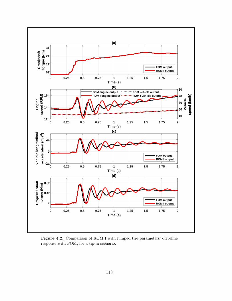
0 0.25 0.5 0.75 1 1.25 1.5 1.75 2Time (s)
0T
1T
2T
3T
Cra
nks
haf
tto
rqu
e (N
m)
(a)
FOM outputROM I output
0 0.25 0.5 0.75 1 1.25 1.5 1.75 2Time (s)
12n
14n
16n
En
gin
esp
eed
(R
PM
)
40
50
60
70
80
Veh
icle
spee
d (
km/h
)
(b)FOM engine outputROM I engine output
FOM vehicle outputROM I vehicle output
0 0.25 0.5 0.75 1 1.25 1.5 1.75 2Time (s)
-2a
0
2a
Veh
icle
lon
git
ud
inal
acce
lera
tio
n (
m/s
2 ) (c)
FOM outputROM I output
0 0.25 0.5 0.75 1 1.25 1.5 1.75 2Time (s)
0
0.4t
0.8t
Pro
pel
ler
shaf
tto
rqu
e (N
m)
(d)
FOM outputROM I output
Figure 4.2: Comparison of ROM I with lumped tire parameters’ drivelineresponse with FOM, for a tip-in scenario.
118

substantial activity in the model. Therefore, the next section deals with including
the tire parameters separately in the ROM.
4.3 ROM with separate tire parameters
4.3.1 ROM II development
Including the tire damping in the equivalent damping coefficient cs, as seen in the
previous sub-section, may be beneficial from a controls perspective. It leads to the
formulation of fewer state variables, thereby reducing the complexity of the controller.
However, it does not replicate the dynamics of the driveline that is observed in the full-
order model, because the effect of tire slip, which is represented by the tire model using
torsional stiffness and damping coefficient, is significant in reducing the oscillations
observed in the driveline. Therefore, in this section, another ROM is developed with
the tire parameters represented separately, as shown in Fig. 4.3.
Figure 4.3: ROM with separate tire parameters.
119

The inputs to the model, and outputs from the model remain similar to the case with
lumped tire parameters. The model equations for this ROM are:
J1θe = Te,inst,brake +Tsitr
(4.4)
J2θv = Tv − Tload (4.5)
Tv = Tsifd (4.6)
Ts = ks(θ1 − θ2) + cs(θ1 + θ2) (4.7)
Tv = kti(θv − θ3) + cti(θv + θ3) (4.8)
120

0 0.25 0.5 0.75 1 1.25 1.5 1.75 2Time (s)
0T
1T
2T
3TC
ran
ksh
aft
torq
ue
(Nm
)
(a)
FOM outputROM II output
0 0.25 0.5 0.75 1 1.25 1.5 1.75 2Time (s)
12n
14n
16n
En
gin
esp
eed
(R
PM
)
40
50
60
70
80
Veh
icle
spee
d (
km/h
)
(b)
FOM engine outputROM II engine output
FOM vehicle outputROM II vehicle output
0 0.25 0.5 0.75 1 1.25 1.5 1.75 2Time (s)
-2a
0
2a
Veh
icle
lon
git
ud
inal
acce
lera
tio
n (
m/s
2 ) (c)
FOM outputROM II output
0 0.25 0.5 0.75 1 1.25 1.5 1.75 2Time (s)
0
0.4t
0.8t
Pro
pel
ler
shaf
tto
rqu
e (N
m)
(d)
FOM outputROM II output
Figure 4.4: Comparison of ROM II with separate tire parameters’ drivelineresponse with FOM, for a tip-in scenario.
121
4.3.2 ROM II validation
The second ROM was also validated against the response of the FOM, for a tip-
in scenario in 5th gear, and the corresponding engine speed, vehicle speed, vehicle
longitudinal acceleration, and propeller shaft torque were plotted. Fig. 4.4 clearly
shows that this ROM is able to match all the parameters of interest, from the FOM,
including the amplitude and frequency of shuffle oscillations.
Similar analysis was carried out for a tip-in scenario in the 3rd gear, and the com-
parison between the FOM and ROM for this case is shown in Fig. 4.5. The response
of the ROM shows a good match in any gear state of the transmission.
4.3.3 Effect of lumping backlashes in the ROM
For both the ROMs discussed in sections 4.2 and 4.3, transmission and final drive
backlash have been lumped together into a single element, taken at the end of the
final drive. Fig. 4.6 shows a comparative analysis of the effect of lumping the backlash
at the final drive on the response of the driveline, during a tip-in scenario, using ROM
with separate tire parameters. Lumping the backlash elements, requires the size of
the backlash to be translated based on the position it is being placed at. For example,
the size of the transmission backlash in the split backlash FOM is assumed to be 10
122
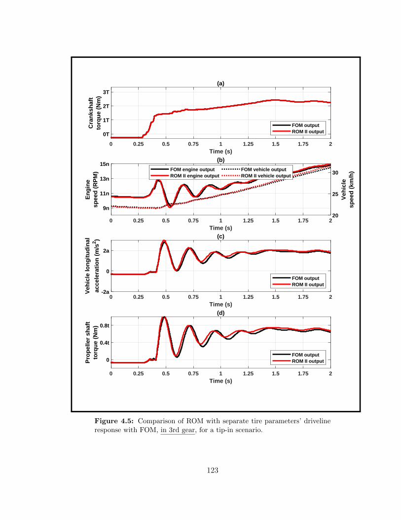
0 0.25 0.5 0.75 1 1.25 1.5 1.75 2Time (s)
0T
1T
2T
3TC
ran
ksh
aft
torq
ue
(Nm
)
(a)
FOM outputROM II output
0 0.25 0.5 0.75 1 1.25 1.5 1.75 2Time (s)
9n
11n
13n
15n
En
gin
esp
eed
(R
PM
)
20
25
30
Veh
icle
spee
d (
km/h
)
(b)
FOM engine outputROM II engine output
FOM vehicle outputROM II vehicle output
0 0.25 0.5 0.75 1 1.25 1.5 1.75 2Time (s)
-2a
0
2a
Veh
icle
lon
git
ud
inal
acce
lera
tio
n (
m/s
2 ) (c)
FOM outputROM II output
0 0.25 0.5 0.75 1 1.25 1.5 1.75 2Time (s)
0
0.4t
0.8t
Pro
pel
ler
shaf
tto
rqu
e (N
m)
(d)
FOM outputROM II output
Figure 4.5: Comparison of ROM with separate tire parameters’ drivelineresponse with FOM, in 3rd gear, for a tip-in scenario.
123

deg., and the size of the final drive backlash is assumed to be 4 deg. But when these
backlashes are lumped at the final drive, the transmission backlash has to be adjusted
for the gear ratios of the transmission, and the final drive, making the lumped element
to have a backlash size of 6 deg. From Fig. 4.6, it is clear that even after lumping
the backlashes at a single element, the ROM is able to capture the frequency and
amplitude of the shuffle oscillations to a satisfactory level of accuracy. As evident
in Fig. 4.6 (b), the rebound in the transmission backlash, after the clunk impact,
observed in the FOM, was not reproduced in the ROM with the lumped backlash.
This has to be taken care of, while developing the controller, so that rebounds in the
backlash elements do not take place.
124

Figure 4.6: Comparison of lumped and split backlash models in full-orderand reduced-order models.
125

4.4 Estimation of model parameters for ROM
For both the ROM’s described in Section 4.2 and 4.3, model parameters like inertias,
stiffnesses and damping coefficients for lumped systems had to be estimated using
available data for the individual components. A brief overview of the methodology
used, for finding the lumped parameters is described in this section.
The engine, torque converter, transmission, propeller shaft, final drive, and the dif-
ferential can be assumed to be in a series connection with one another. After the
differential, the axle shafts on the left side, and right side of the driveline, and the
tires on the left side, and right side of the driveline, can be assumed to be parallel to
their respective element. After lumping the left and right side axle shaft, and tire,
the lumped elements are assumed to be in series again.
Irrespective of the assumed connections, the equivalent moment of inertia is obtained
by simply adding the inertias together. If there is a gear ratio (e.g. transmission gear
ratio, final drive gear ratio) between two inertias that need to be lumped, then the
square of the gear ratio was considered while calculating the lumped inertia. As an
example, the procedure for lumping moment of inertias of the propeller shaft, axle
shafts, and the tires is shown:
126
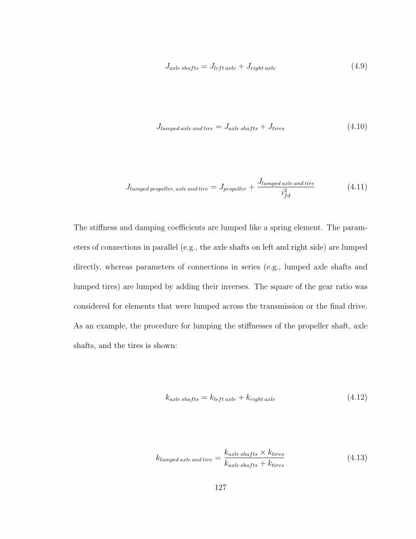
Jaxle shafts = Jleft axle + Jright axle (4.9)
Jlumped axle and tire = Jaxle shafts + Jtires (4.10)
Jlumped propeller, axle and tire = Jpropeller +Jlumped axle and tire
i2fd(4.11)
The stiffness and damping coefficients are lumped like a spring element. The param-
eters of connections in parallel (e.g., the axle shafts on left and right side) are lumped
directly, whereas parameters of connections in series (e.g., lumped axle shafts and
lumped tires) are lumped by adding their inverses. The square of the gear ratio was
considered for elements that were lumped across the transmission or the final drive.
As an example, the procedure for lumping the stiffnesses of the propeller shaft, axle
shafts, and the tires is shown:
kaxle shafts = kleft axle + kright axle (4.12)
klumped axle and tire =kaxle shafts × ktireskaxle shafts + ktires
(4.13)
127

klumped propeller, axle and tire =
kpropeller ×klumped axle and tire
i2fd
kpropeller +klumped axle and tire
i2fd
(4.14)
For lumping the damping coefficients, the same procedure used in Eq. 4.12, 4.13 and
4.14 was used.
4.5 Application of ROM for controls
The ROM with separate tire parameters will later be used for developing an esti-
mator and a controller for reducing the shuffle oscillations. The estimator will help
in estimating backlash states in the driveline, whereas the controller will shape the
torque trajectory to reduce impact at gear faces after backlash traversal.
Figure 4.7: Schematic showing a simple control system, utilizing the outputof the ROM, for controlling the torque delivered to the plant(Full-ordermodel).
128

A simple controls application of the ROM in reducing the shuffle oscillations is demon-
strated here. The schematic of this simple control system is shown in Fig. 4.7. The
torque requested by the driver, through the accelerator pedal, is received as a com-
mand signal by the controller, as well as the ROM. Based on the driver requested
torque, the ROM estimates the position of the backlash continuously. When the back-
lash is in either negative contact, or positive contact, the controller does not modify
the torque requested by the driver. As soon as the backlash traversal starts to take
place in the ROM, the status of the backlash becomes inlash, and a signal is sent to
the controller. The controller, then uses a multiplication factor to reduce the ramp
rate of driver requested torque, which is sent to the virtual plant, represented by the
full-order model for showing this result. To avoid the torque request from increas-
ing rapidly after backlash traversal, the multiplication factor is integrated with time,
which leads to a smooth increase in torque. This approach is used based on the effect
observed in Chapter 3, of reduced driveline oscillation amplitude, with a reduction in
ramp rate of torque input, and learnings from [46]. The mathematical equation for
the approach used is shown below:
dTshaped(t)
dt= Tdriver(t)
∫ 1
0.05
F (t)dt (4.15)
where, Tshaped is the shaped engine torque, Tdriver is the driver requested torque, and
F is the multiplication factor that is used for reducing the ramp rate of the delivered
129

torque.
Fig. 4.8 shows a comparative response of the driveline oscillations in the virtual plant
for two cases. In case A, torque output from the engine is obtained from the driver
requested torque, and therefore, it is not externally shaped by the controller. The
trajectory of torque output observed in case A, is due to the air charge dynamics
discussed in Chapter 2. Consequently, the amplitude of shuffle oscillations is higher,
as seen in propeller shaft torque and vehicle longitudinal acceleration. In case B, the
torque output from the engine is shaped, based on the input received from the ROM,
about the status of the backlash. Since, the torque shaping reduces the ramp rate
of the engine output torque, a 53% reduction in amplitude of oscillations of vehicle
acceleration is observed. Moreover, the backlash traversal time also increases in both
the transmission and final drive backlash. This demonstrates the ability of the ROM
for controls applications.
130

9 9.5 10 10.5 11 11.5 12Time (s)
0
100
200
300C
ran
ksh
aft
torq
ue
(Nm
)
(a)
Driver requested torqueTorque output - Case ATorque output - Case B
9 9.5 10 10.5 11 11.5 12Time (s)
0
200
400
Sh
aft
torq
ue
(Nm
)
(b)
Propeller shaft torque - Case A Propeller shaft torque - Case B
9 9.5 10 10.5 11 11.5 12Time (s)
-1
-0.5
0
0.5
1
1.5
Veh
icle
lon
git
ud
inal
acce
lera
tio
n (
m/s
2 ) (c)
Vehicle acceleration - Case AVehicle acceleration - Case B
9 9.5 10 10.5 11 11.5 12Time (s)
-5
0
5
Bac
klas
htr
aver
sal (
deg
.)
(d)
Transmission backlash - Case ATransmission backlash - Case BFinal drive backlash - Case AFinal drive backlash - Case B
Figure 4.8: Comparison of driveline response for two cases of torque input.Case A: Torque input without shaping. Case B: Torque input with shaping.
131


Chapter 5
Conclusion and Future work
5.1 Conclusions
† A full-order model of a current generation vehicle based on an SUV/pick-
up truck platform was developed, using an Amesim® - Simulink® interface.
Model parameters for the powertrain were provided by the sponsoring organi-
zation. Literature review was carried out in modeling and controls domain for
simulating and reducing driveline oscillations during tip-in and tip-out scenarios
in automobiles.
† The actual torque delivered by an engine is bound to have an error, compared
to the ECU estimated values, due to the reasons discussed in Chapter 2. It
133

is essential to take this error into account since the ramp rate of the delivered
torque, directly affects the magnitude of driveline oscillations.
† The developed model was validated for three different use modes: (i) locked
torque converter clutch, (ii) open torque converter clutch and (iii) slipping
torque converter clutch. Experimental data was collected and provided by the
sponsoring organization, for tip-in and tip-out scenarios. Some of the observa-
tions made during model validation were:
– For the case of a locked TCC, the parameters of the developed full-order
model had to be modified, in order to match the behavior of the driveline,
during tip-in condition, as observed in the experimental data. The stiffness
of the propeller and axle shafts had to be reduced by 25%, and the inertia
of the engine, torque converter, and final node of the transmission had to
be increased by 25%, to account for the components that could not be
modeled due to lack of parametric data, but which had an impact on the
oscillation frequency.
– For the scenarios where the flow of torque in a torque converter, takes
place in either the fluid path or in a combination of fluid and lock-up
clutch path, a simple look-up table for capacity factor and torque ratio,
as a function of speed ratio, is not enough to capture the dynamics inside
the torque converter during transient events like tip-in. A detailed model
which takes into account the geometrical parameters like number of blades,
134

blade angles etc., and fluid flow properties, is required for replicating the
dynamics inside the torque converter accurately during transient scenarios.
† Parametric analysis was performed on the full-order model, to analyze the effect
of elements such as backlashes, shaft stiffnesses etc., on driveline oscillations.
The results are summarized below:
– The ramp rate of the provided torque input is a prime factor that affects the
amplitude of the shuffle oscillations that are induced due to both backlash
and shaft flexibility. A higher ramp rate leads to a higher amplitude of
oscillation and vice-versa.
– The effect of variation in the final drive backlash size is more significant
on the shuffle oscillation amplitude, compared to a similar variation in the
transmission backlash.
– The effect of variation of axle shaft stiffness is more significant on the
shuffle frequency, compared to a similar variation in the propeller shaft.
There is no influence on the amplitude of shuffle oscillations in either case.
– The effect of variation in damping coefficient of both propeller and axle
shafts is negligible on the frequency and amplitude of shuffle oscillations,
which is due to their low contribution, in the overall damping of the system.
† The full-order model was simplified into a reduced-order model, to be used in
controls work in the future. Two reduced-order model designs were investigated,
135

based on the how the tire parameters were considered in the model. Some of
the findings are:
– It is necessary to include the tire parameters as a separate entity in the
model, for retaining most of the fidelity of the full-order model. Lumping
the tire parameters within the model might still provide some insight into
the behavior of the actual vehicle’s driveline, but it may not be useful for
developing precise controls.
– Lumping the backlashes at the transmission and the final drive into a
single element might make it easier to develop and implement an effective
estimator and controller in future, but it might not be able to accurately
replicate driveline scenarios where the driver requests a small amount of
torque for a short period of time, causing the transmission backlash to
traverse, but not the final drive backlash. It is important to take that into
account, so that the developed control system can take the required steps
to mitigate such driveline clunk scenarios.
– Implementing the developed ROM in a simple control system, with the
full-order model as a virtual plant, showed the application capability of
the ROM. Using a simple, factor-based torque shaping technique, drive-
line oscillation amplitude was successfully reduced by 53.44 % in vehicle
longitudinal acceleration.
136
5.2 Future work
While this work was based on the effect of backlash traversal and shaft flexibility
for inducing shuffle oscillations, the model can be improved for studying the effect
of road disturbances on the driveline. Similarly, the tire model can be modified for
studying the effect of sudden variations in road friction on the driveline. Considering
the main objective of the current thesis, the future work includes:
† Verifying the validity of some of the assumed model parameters to further im-
prove the accuracy of the full-order and reduced-order models. This will be
accomplished through an ongoing Ph.D. thesis at Michigan Tech.
† Development and validation of a dynamic torque converter model, such that
transient events can be accurately replicated, during the slipping and open
modes of the torque converter lock-up clutch.
† Development and validation of state estimators, based on Kalman filtering tech-
niques, such that backlash state and position can be estimated in real-time,
without having to rely on alternative algorithms to provide an approximation.
† Sensitivity analysis of vehicle parameters that can vary due to the availability
of different model variants of a vehicle, e.g., mass of the vehicle, overall iner-
tia of the vehicle, tire properties of the vehicle etc., on driveline oscillations.
137

Parameters having significant impact will be included with parameters to be
estimated using state estimators.
† Development and validation of a robust model-based anti-jerk controller, that
can utilize the outputs from the state estimator, and shape the torque to be
delivered in such a way that the impact velocity at the end of backlash traver-
sal is significantly reduced, and therefore the NHV characteristics of the vehi-
cle are improved. The controller will need to be robust to changes in vehicle
parameters, without requiring additional calibration, thereby reducing current
calibration time and effort.
† Analysis of effect of tire slip on driveline oscillations, and possible integration
of strategies for both slip-induced and backlash-induced jerk control.
† Implementation of the estimator and the controller on a test rig, which is cur-
rently under development at Michigan Tech, to study their effectiveness during
actual drive scenarios.
138
References
[1] Cain, T., 2017. U.S. auto sales in calendar year 2016, by
vehicle category. http://www.goodcarbadcar.net/2017/01/
usa-auto-sales-by-vehicle-type-2016-char/. Accessed on 8 January
2018, [Online].
[2] PwC, 2017. Projected vehicle sales in China, the U.S. and the
EU between 2017 and 2030, by propulsion technology (in mil-
lion vehicles). https://www.statista.com/statistics/264754/
worldwide-vehicle-sales-by-propulsion-technology-2025/. Accessed on
8 January 2018, [Online].
[3] &, S., and PwC, 2017. Projected sales of autonomous vehicles, classified
by level of automation. https://www.strategyand.pwc.com/media/file/
2017-Strategyand-Digital-Auto-Report.pdf. Accessed on 8 January 2018,
[Online].
139

[4] GearHeads, 2010. Backlash. Used under Creative Commons Attribution-Share
Alike 3.0 Unported license.
[5] Papageorgiou, D., Blanke, M., Niemann, H. H., and Richter, J. H., 2017. “Back-
lash estimation for industrial drive-train systems”. IFAC-PapersOnLine, 50(1),
pp. 3281–3286.
[6] Baumann, J., Torkzadeh, D. D., Ramstein, A., Kiencke, U., and Schlegl, T.,
2006. “Model-based predictive anti-jerk control”. Control Engineering Practice,
14(3), pp. 259–266.
[7] Grotjahn, M., Quernheim, L., and Zemke, S., 2006. “Modelling and identifi-
cation of car driveline dynamics for anti-jerk controller design”. In 2006 IEEE
International Conference on Mechatronics. Budapest, Hungary.
[8] Lagerberg, A., and Egardt, B., 2002. “Evaluation of control strategies for au-
tomotive powertrains with backlash”. In 6th International Symposium on Ad-
vanced Vehicle Control. Hiroshima, Japan.
[9] Lagerberg, A., and Egardt, B., 2007. “Backlash estimation with application to
automotive powertrains”. IEEE Transactions on Control Systems Technology,
15(3), pp. 483–493.
[10] Lagerberg, A., and Egardt, B., 2005. “Model predictive control of automotive
powertrains with backlash”. In IFAC Proceedings Volumes, Vol. 38, pp. 1–6.
140

[11] Templin, P., and Egardt, B., 2011. “”A powertrain LQR-torque compensator
with backlash handling””. Oil & Gas Science and Technology–Revue dIFP En-
ergies nouvelles, 66(4), pp. 645–654.
[12] Baumann, J., Swarnakar, A., Kiencke, U., and Schlegl, T., 2005. “A robust
controller design for anti-jerking”. SAE Technical Paper 2005-01-0041.
[13] Siemens Industry Software NV, 2017. LMS Amehelp - User Manual for
LMS.Amesim 15.2. LMS.Amesim, Plano, TX.
[14] Goleski, G. D., and Thomas, S. G., 2014. Paths for supplying fluid to clutches
of an automatic transmission, Sept. 16. US Patent 8,834,310.
[15] Oman, C. M., 1990. “Motion sickness: a synthesis and evaluation of the sensory
conflict theory”. Canadian journal of physiology and pharmacology, 68(2),
pp. 294–303.
[16] Griffin, M. J., 2012. Handbook of human vibration. Academic press.
[17] Crowther, A. R., Zhang, N., and Singh, R., 2005. “Development of a clunk
simulation model for a rear wheel drive vehicle with automatic transmission”.
SAE Technical Paper 2005-01-2292.
[18] Lagerberg, A., and Egardt, B., 2003. “Estimation of backlash with application to
automotive powertrains”. In Proceedings of 42nd IEEE International Conference
on Decision and Control. Maui, HI, USA.
141

[19] Cho, D., and Hedrick, J. K., 1989. “Automotive powertrain modeling for con-
trol”. Journal of dynamic systems, measurement, and control, 111(4), pp. 568–
576.
[20] Hrovat, D., and Tobler, W., 1991. “Bond graph modeling of automotive power
trains”. Journal of the Franklin Institute, 328(5-6), pp. 623–662.
[21] Pettersson, M., 1997. Driveline modeling and control. Department of Electrical
Engineering, Linkoping University.
[22] Hayat, O., Lebrun, M., and Domingues, E., 2003. “Powertrain driveability eval-
uation: analysis and simplification of dynamic models”. SAE Technical paper
2003-01-1328.
[23] Karlsson, J., and Fredriksson, J., 1999. “Cylinder-by-cylinder engine models
vs mean value engine models for use in powertrain control applications”. SAE
Technical Paper 1999-01-0906.
[24] Sorniotti, A., 2008. “Driveline modeling, experimental validation and evaluation
of the influence of the different parameters on the overall system dynamics”.
SAE Technical Paper 2008-01-0632.
[25] Bartram, M., Mavros, G., and Biggs, S., 2010. “A study on the effect of road
friction on driveline vibrations”. Proceedings of the Institution of Mechanical
Engineers, Part K: Journal of Multi-body Dynamics, 224(4), pp. 321–340.
142

[26] Dridi, S., Salem, I. B., and El Amraoui, L., 2017. “Dynamic modeling of non-
linear longitudinal automotive system using graphically based techniques”. In
Information and Digital Technologies (IDT), 2017 International Conference on,
IEEE, pp. 349–354.
[27] Sun, G., Wei, M., Shao, J., and Pei, M., 2007. “Automotive powertrain modeling
and simulation based on amesim”. SAE Technical Paper 2007-01-3464.
[28] Lagerberg, A., 2001. “A literature survey on control of automotive powertrains
with backlash”. Technical report no R013/2001; Department of Signals and
Systems, Chalmers University of Technology, Gothenburg, Sweden, pp. 1–15.
[29] Templin, P., 2008. “Simultaneous estimation of driveline dynamics and backlash
size for control design”. In IEEE International conference on Control Applica-
tions. San Antonio, Texas, USA.
[30] Templin, P., and Egardt, B., 2009. “”An LQR torque compensator for drive-
line oscillation damping””. In IEEE Conference on Control Applications. St.
Petersburg, Russia.
[31] Karikomi, T., Itou, K., Okubo, T., and Fujimoto, S., 2006. “Development of the
shaking vibration control for electric vehicles”. In 2006 SICE-ICASE Interna-
tional Joint Conference. Busan,Korea.
[32] Kawamura, H., Ito, K., Karikomi, T., and Kume, T., 2011. “Highly-responsive
143
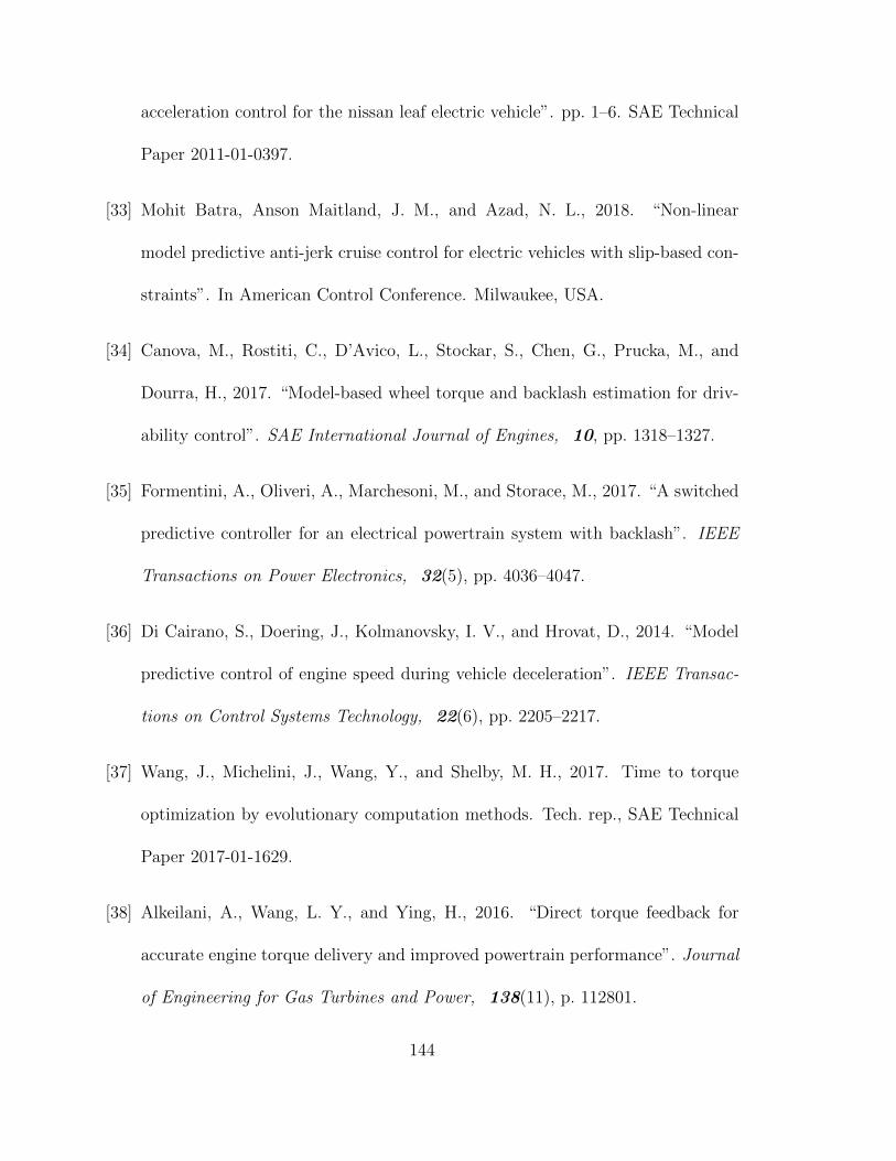
acceleration control for the nissan leaf electric vehicle”. pp. 1–6. SAE Technical
Paper 2011-01-0397.
[33] Mohit Batra, Anson Maitland, J. M., and Azad, N. L., 2018. “Non-linear
model predictive anti-jerk cruise control for electric vehicles with slip-based con-
straints”. In American Control Conference. Milwaukee, USA.
[34] Canova, M., Rostiti, C., D’Avico, L., Stockar, S., Chen, G., Prucka, M., and
Dourra, H., 2017. “Model-based wheel torque and backlash estimation for driv-
ability control”. SAE International Journal of Engines, 10, pp. 1318–1327.
[35] Formentini, A., Oliveri, A., Marchesoni, M., and Storace, M., 2017. “A switched
predictive controller for an electrical powertrain system with backlash”. IEEE
Transactions on Power Electronics, 32(5), pp. 4036–4047.
[36] Di Cairano, S., Doering, J., Kolmanovsky, I. V., and Hrovat, D., 2014. “Model
predictive control of engine speed during vehicle deceleration”. IEEE Transac-
tions on Control Systems Technology, 22(6), pp. 2205–2217.
[37] Wang, J., Michelini, J., Wang, Y., and Shelby, M. H., 2017. Time to torque
optimization by evolutionary computation methods. Tech. rep., SAE Technical
Paper 2017-01-1629.
[38] Alkeilani, A., Wang, L. Y., and Ying, H., 2016. “Direct torque feedback for
accurate engine torque delivery and improved powertrain performance”. Journal
of Engineering for Gas Turbines and Power, 138(11), p. 112801.
144

[39] Schwab, M., 1990. “Electronically-controlled transmission systems-current posi-
tion and future developments”. In Vehicle Electronics in the 90’s: Proceedings of
the International Congress on Transportation Electronics, 1990, IEEE, pp. 335–
342.
[40] Pacejka, H. B., and Bakker, E., 1992. “The magic formula tire model”. Vehicle
System Dynamics, 21(sup001), pp. 1–18.
[41] Mozharovskii, V. V., Shil’ko, S. V., Anfinogenov, S. B., and Khot’ko, A. V.,
2007. “Determination of resistance to rolling of tires in dependence on operating
conditions. part 1. method of multifactorial experiment”. Journal of Friction
and Wear, 28(2), Apr, pp. 154–161.
[42] Pscoa, J., Brojo, F., Charrua Santos, F., and Fael, P., 2012. “An innovative
experimental on-road testing method and its demonstration on a prototype ve-
hicle”.
[43] Toolbox, E., 2008. Rolling resistance. https://www.engineeringtoolbox.com/
rolling-friction-resistance-d_1303.html. (Accessed on 16 July, 2018).
[Online].
[44] Lagerberg, A., 2004. “Control and estimation of automotive powertrains with
backlash”. PhD thesis, Chalmers University of Technology, Sweden.
[45] Hao, D., Zhao, C., and Huang, Y., 2018. “A reduced-order model for active
145

suppression control of vehicle longitudinal low-frequency vibration”. Shock and
Vibration, 2018.
[46] Krenz, R., 1985. “Vehicle response to throttle tip-in/tip-out”. pp. 45–52. SAE
Technical Paper 850967.
146

Appendix A
Amesim-Simulink Interface
For setting up the interface between Amesim and Simulink, specific versions of their
packages had to be used with Visual C++ compiler. At the time of writing this
thesis, the following versions of the softwares were being used:
LMS Amesim:
Version → 15.2 (63896-58725) 2017
Platform → Windows 7/8/10
Library → Standard Amesim library
MATLAB/Simulink:
Version → MATLAB - 9.4.0.885841 (R2018a) Update 3
→ Simulink - 9.1 (R2018a)
147

Microsoft Visual Studio:
Version → 12.0.21005.1 REL
Microsoft Visual C++:
Version → 2013
Code to load Amesim libraries in Simulink
>addpath(fullfile(getenv(’AME’),’scripting’,’matlab’,’amesim’));
>ameml
148

Appendix B
Engine Torque Uncertainty
After reviewing the results of the torque measurements, that were carried out by the
sponsoring organization, for various tip-in and tip-out conditions, it was found that
using a fixed transfer function for representing the dynamics of air flow into the cylin-
ders is not adequate. Variations in the experimentally observed torque trajectories
were significant, and to simplify replication of those variations, torque calculations
by the engine model in this work include a term Tunc.
Four different scenarios are shown here, which include one tip-in scenario with rel-
atively small driver torque request, one tip-in scenario with relatively large driver
torque request, one tip-in scenario with maximum driver torque request, and one
tip-out scenario. The transfer function used in each scenario is mentioned on the
plots.
149

Figure B.1: Observed engine torque response for a throttle input of 0 →100%
Figure B.2: Observed engine torque response for a throttle input of 0 →60%
150

Figure B.3: Observed engine torque response for a throttle input of 0 →20%
Figure B.4: Observed response for a throttle tip-out scenario
151

Each of the plot in Fig. B.1 - Fig. B.4 shows flexplate brake torque, which is adapted
from the experimental data that the sponsoring organization shared, requested brake
torque, which was the assumed simulation input for the engine model, instantaneous
brake torque and instantaneous brake torque with error included, which are the ob-
served outputs of the engine model for the transfer functions mentioned on the plots.
152

Appendix C
Program and Data File Summary
Following image and model files were used for this thesis, organized as per the chapter
they were used in:
C.1 Chapter 1
Table C.1Chapter 1 figure files
File name File description
Fig 1 1.jpg Figure 1.1Fig 1 2.jpg Figure 1.2Fig 1 3.jpg Figure 1.3Fig 1 4.vsdx Figure 1.4Fig 1 5.jpg Figure 1.5Fig 1 6.bmp Figure 1.6Fig 1 7.bmp Figure 1.7Fig 1 8.bmp Figure 1.8Fig 1 9.bmp Figure 1.9Fig 1 10.vsdx Figure 1.10
153

C.2 Chapter 2
Table C.2Chapter 2 figure files
File name File description
Fig 2 1.vsdx Figure 2.1Fig 2 2.bmp Figure 2.2Fig 2 3.bmp Figure 2.3Fig 2 4.jpg Figure 2.4Fig 2 5.jpg Figure 2.5Fig 2 6.bmp Figure 2.6Fig 2 7.jpg Figure 2.7Fig 2 8.jpg Figure 2.8Fig 2 9.jpg Figure 2.9Fig 2 10.vsdx Figure 2.10Fig 2 11.fig Figure 2.11Fig 2 12.fig Figure 2.12Fig 2 13.fig Figure 2.13Fig 2 14.fig Figure 2.14Fig 2 15.fig Figure 2.15Fig 2 16.fig Figure 2.16Fig 2 17.fig Figure 2.17Fig 2 18.fig Figure 2.18Fig 2 19.fig Figure 2.19Fig 2 20.fig Figure 2.20
Table C.3Chapter 2 model files
File name File description
Driveline model final.ame Amesim file of full-order driveline modelTorque shaping final model.slx Simulink file of engine modelPlot code model validation lockedTCC.m Code for model validation graphs
of locked TCCPlot code model validation openTCC.m Code for model validation graphs
of open TCCPlot code model validation slippingTCC.m Code for model validation graphs
of slipping TCC
154
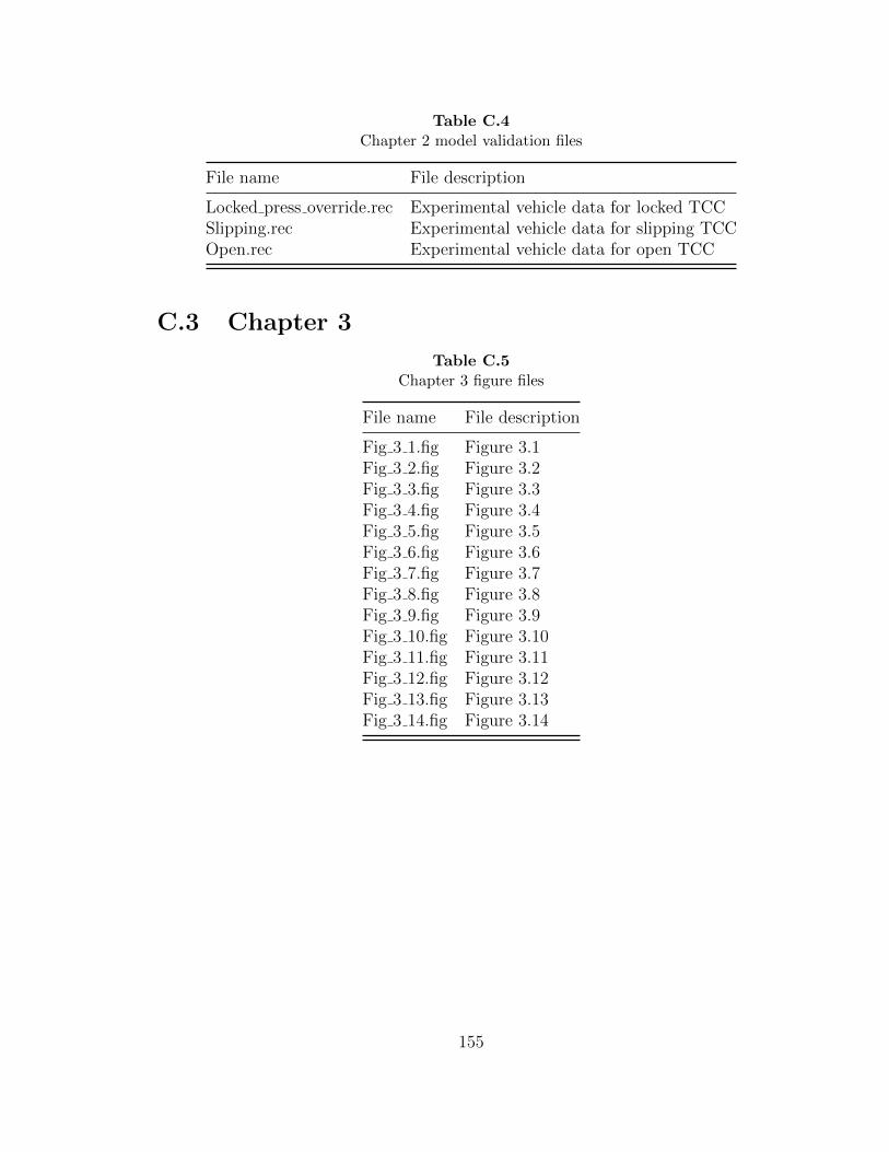
Table C.4Chapter 2 model validation files
File name File description
Locked press override.rec Experimental vehicle data for locked TCCSlipping.rec Experimental vehicle data for slipping TCCOpen.rec Experimental vehicle data for open TCC
C.3 Chapter 3
Table C.5Chapter 3 figure files
File name File description
Fig 3 1.fig Figure 3.1Fig 3 2.fig Figure 3.2Fig 3 3.fig Figure 3.3Fig 3 4.fig Figure 3.4Fig 3 5.fig Figure 3.5Fig 3 6.fig Figure 3.6Fig 3 7.fig Figure 3.7Fig 3 8.fig Figure 3.8Fig 3 9.fig Figure 3.9Fig 3 10.fig Figure 3.10Fig 3 11.fig Figure 3.11Fig 3 12.fig Figure 3.12Fig 3 13.fig Figure 3.13Fig 3 14.fig Figure 3.14
155
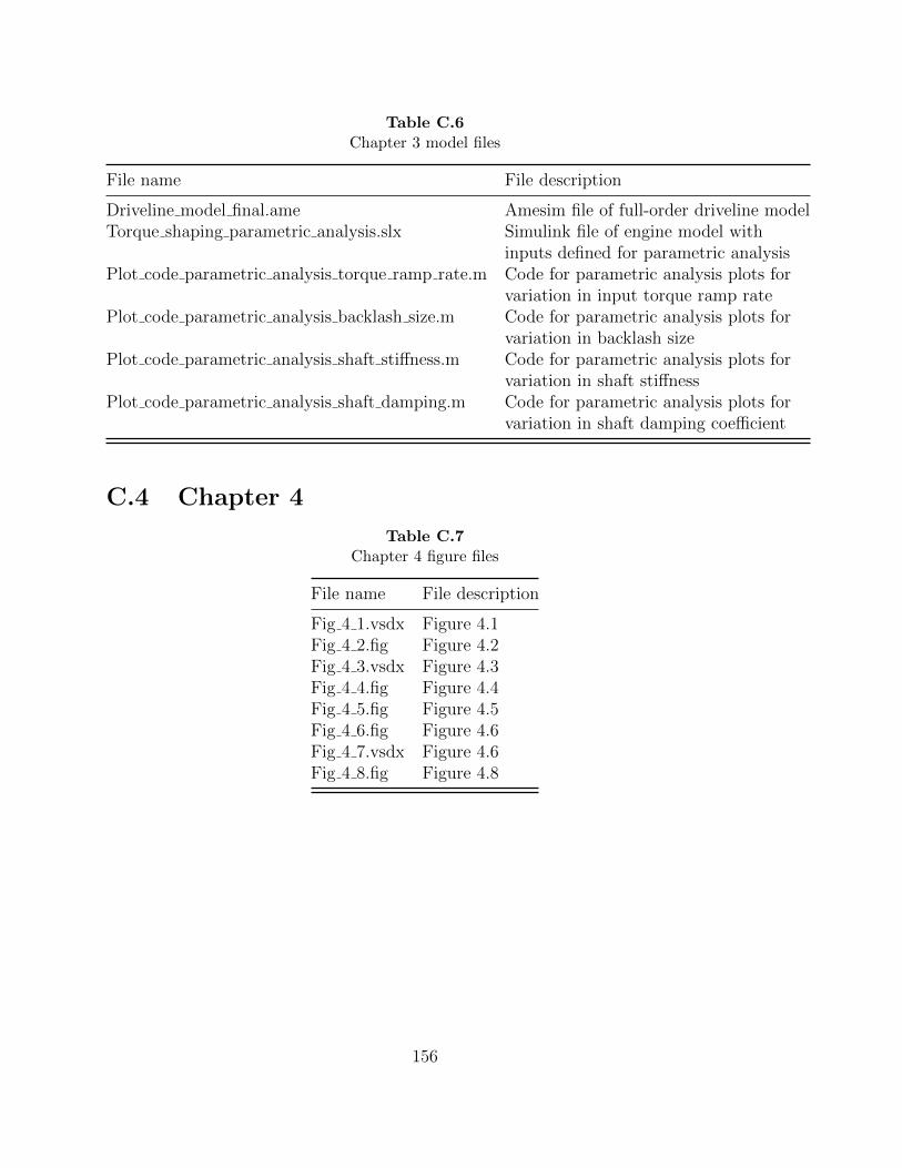
Table C.6Chapter 3 model files
File name File description
Driveline model final.ame Amesim file of full-order driveline modelTorque shaping parametric analysis.slx Simulink file of engine model with
inputs defined for parametric analysisPlot code parametric analysis torque ramp rate.m Code for parametric analysis plots for
variation in input torque ramp ratePlot code parametric analysis backlash size.m Code for parametric analysis plots for
variation in backlash sizePlot code parametric analysis shaft stiffness.m Code for parametric analysis plots for
variation in shaft stiffnessPlot code parametric analysis shaft damping.m Code for parametric analysis plots for
variation in shaft damping coefficient
C.4 Chapter 4
Table C.7Chapter 4 figure files
File name File description
Fig 4 1.vsdx Figure 4.1Fig 4 2.fig Figure 4.2Fig 4 3.vsdx Figure 4.3Fig 4 4.fig Figure 4.4Fig 4 5.fig Figure 4.5Fig 4 6.fig Figure 4.6Fig 4 7.vsdx Figure 4.6Fig 4 8.fig Figure 4.8
156

Table C.8Chapter 4 model files
File name File description
Driveline model ROM.ame Amesim file of reduced-order driveline modelTorque shaping final model.slx Simulink file of engine modelTorque shaping ROM model.slx Simulink file ROM controlsPlot code ROM validation.m Code for validation of ROM with FOMPlot code ROM controls.m Code for comparison of ROM in controls
C.5 Appendix B
Table C.9Appendix B figure files
File name File description
Fig B 1.bmp Figure B.1Fig B 2.bmp Figure B.2Fig B 3.bmp Figure B.3Fig B 4.bmp Figure B.4
157