CONTROL OF INFINITE DIMENSIONAL SYSTEMS USING FINITEDIMENSIONAL TECHNIQUES: A SYSTEMATIC APPROACH

byArmando Antonio Rodriguez

B.S., Electrical Engineering, Polytechnic Institute of New York(1983)

S.M., Electrical Engineering, Massachusetts Institute of Technology(1987)

E.E., Electrical Engineering, Massachusetts Institute of Techmology(1989)

Submitted to the Department of

ELECTRICAL ENGINEERING AND COMPUTER SCIENCE

in partial fulfillment of the requirements for the degree of

DOCTOR OF PHILOSOPHY

at the

MASSACHUSETTS INSTITUTE OF TECHNOLOGY

August 1990

@Armando Antonio Rodriguez, 1990

The author hereby grants permission to M.I.T to reproduce and to distribute copies of this thesisdocument in whole or in part

Signature of Author:.............. - ........ .

Department of Electrical Engineering anVComputer ScienceA -

Certified by: ......................................

leh

sor__

Accepted by: ................................................ ............

Arthur C. Smith, ChairmanMASSACHUSETTS INSTITUTE

OF TECHNOLOGY

NOV 27 1990

,ARARIESARCHIVES

Committee on Graduate Students

Report Documentation Page Form ApprovedOMB No. 0704-0188

Public reporting burden for the collection of information is estimated to average 1 hour per response, including the time for reviewing instructions, searching existing data sources, gathering andmaintaining the data needed, and completing and reviewing the collection of information. Send comments regarding this burden estimate or any other aspect of this collection of information,including suggestions for reducing this burden, to Washington Headquarters Services, Directorate for Information Operations and Reports, 1215 Jefferson Davis Highway, Suite 1204, ArlingtonVA 22202-4302. Respondents should be aware that notwithstanding any other provision of law, no person shall be subject to a penalty for failing to comply with a collection of information if itdoes not display a currently valid OMB control number.

1. REPORT DATE AUG 1990 2. REPORT TYPE

3. DATES COVERED 00-00-1990 to 00-00-1990

4. TITLE AND SUBTITLE Control of Infinite Dimensional Systems Using Finite DimensionalTechniques: A Systematic Approach

5a. CONTRACT NUMBER

5b. GRANT NUMBER

5c. PROGRAM ELEMENT NUMBER

6. AUTHOR(S) 5d. PROJECT NUMBER

5e. TASK NUMBER

5f. WORK UNIT NUMBER

7. PERFORMING ORGANIZATION NAME(S) AND ADDRESS(ES) Massachusetts Institute of Technology,77 Massachusetts Avenue,Cambridge,MA,02139

8. PERFORMING ORGANIZATIONREPORT NUMBER

9. SPONSORING/MONITORING AGENCY NAME(S) AND ADDRESS(ES) 10. SPONSOR/MONITOR’S ACRONYM(S)

11. SPONSOR/MONITOR’S REPORT NUMBER(S)

12. DISTRIBUTION/AVAILABILITY STATEMENT Approved for public release; distribution unlimited

13. SUPPLEMENTARY NOTES

14. ABSTRACT

15. SUBJECT TERMS

16. SECURITY CLASSIFICATION OF: 17. LIMITATION OF ABSTRACT Same as

Report (SAR)

18. NUMBEROF PAGES

135

19a. NAME OFRESPONSIBLE PERSON

a. REPORT unclassified

b. ABSTRACT unclassified

c. THIS PAGE unclassified

Standard Form 298 (Rev. 8-98) Prescribed by ANSI Std Z39-18

Control of Infinite Dimensional Systems using Finite Dimensional Techniques: ASystematic Approach

by: Armando Antonio Rodriguez

Submitted to the Department of Electrical Engineering and Computer Science on August 15, 1990in partial fulfillment of the requirements for the degree of Doctor of Philosophy.

ABSTRACT

In this thesis, the problem of designing finite dimensional controllers for infinite dimensionalsingle-input single-output systems is addressed. More specifically, it is shown how to systematicallyobtain near-optimal finite dimensional compensators for a large class of scalar infinite dimensionalplants. The criteria used to determine optimality are standard H** and ?X2 weighted sensitivityand mixed-sensitivity measures.

Unlike other approaches which appear in the literature, the approach taken here avoids solv-ing an infinite dimensional optimization problem to get an infinite dimensional compensator andthen approximating to get an appropriate finite dimensional compensator. Rather than this De-sign/Approximate approach, we take an Approximate/Design approach. In this approach one startswith a "good" finite dimensional approximant for the infinite dimensional plant and then solves afinite dimensional optimization problem to get a suitable finite dimensional compensator. Tradi-tionally, however, this approach has not come with any guarantees.

The key difficulties which have arisen can be attributed to the fact that these measures aresometimes not continuous with respect to plant perturbations, even when the uniform topology isimposed. Moreover, even if they were, it is a known fact that many interesting infinite dimensionalplants can not be approximated in the uniform topology on -Oo (e.g. a delay). Also, it must benoted that the concept of a "good" approximant, in the context of feedback design, has never beenrigorously formulated.

The goal and main contribution of this research endeavour has been to resolve these difficulties.It is shown that given a "suitable" finite dimensional approximant for an infinite dimensionalplant, one can solve a "natural" finite dimensional problem in order to obtain a near-optimal finitedimensional compensator. Moreover, very weak conditions are presented to indicate what a "good"approximant is.

In addition, we show that the optimal performance for a large class of W11o design paradigms canbe computed by solving a sequence of finite dimensional eigenvalue/eigenvector problems ratherthan the typical infinite dimensional eigenvalue/eigenfunction problems which appear in the liter-ature. Analogous results are presented for a large class of H2 paradigms.

In summary, the approach taken here allows one to forgo solving "complex" infinite dimensionalproblems and provides rigorous justification for some of the approximations that control engineerstypically make in practice.

Thesis Supervisor: Dr. Munther A. DahlehTitle: Professor of Electrical Engineering & Computer Science

Acknowlegdements

First and foremost, I would like to thank my thesis supervisor, Professor Munther Dahleh. Hehas always offered infinite support, both technical and otherwise. His guidance, patience, and deepconcern have been very much appreciated. I have been extremely fortunate to have had him as mythesis supervisor. I cannot thank him enough. I feel lucky not only to have had the opportunityto learn from him, as a student, but also to have associated with him as a person. Although I willsee him at conferences in the future, I will still miss him a great deal.

I would also like to thank my thesis committee members Dr. Gunter Stein and Professor SanjoyMitter for their helpful consultation throughout the course of this research. Every session withthem provided perspective and great insight. It was a pleasure and an honor to work with them.

In addittion, I must thank Professor Michael Athans, Ignacio Diaz-Bobillo, Joel Douglas, Profes-sor David Flamm, Dr. Petros Kapasouris, Sanjeev Kulkarni, Joseph Lutsky, Dr. Dragan Obradovid,Professor Jason Papastavrou, Dr. Tom Richardson, Professor Brett Ridgely, Professor Jeff Shamma,Petros Voulgaris, Jim Walton. All have contributed in some way or form.

The staff at LIDS was always helpful and supportive. I would particularly like to thank FifaMonserrate. She was always kind, warm, and cheerful.

I must also give great thanks to AT&T Bell Laboratories for their most generous fellowship.I would like to specifically thank my mentor at the labs, Dr. Sid Ahuja. He has always beensupportive.

Finally, I must give special thanks to my father and my brothers David and Raul for the love,encouragement, and support that they have given me over the years. I would also like to thankmy dear friend Ted Hernandez who unfortunately passed away during this last year. I owe him somuch.

This research was conducted at the M.I.T Laboratory for Information and Decision Systems.It has been supported by AT&T Bell Laboratories, by the Center for Intelligent Control Systemsunder the Army Research Office grant DAAL03-86-K-0171, and by NSF grant 8810178-ECS.

To my father.

Contents

1 Introduction & Overview1.1 M otivation . . . . . . . . . . . . . . . . .1.2 Related Work & Previous Literature . . .1.31.4

Contributions of Thesis . . . . . . .Organization of Thesis . . . . . . . .

2 Mathematical Preliminaries: Notation &2.1 Introduction . . . . . . . . . . . . . . . . .2.2 Some Notation & Definitions . . . . . . .2.3 Single-Valued Complex Functions . . . . .2.4 Multi-Valued Complex Functions . . . . .2.5 L2 Function Theory . . . . . . . . . . . .2.6 Cw Function Theory . . . . . . . . . . . .2.7 H** Function Theory . . . . . . . . . . . .2.8 Theory of Linear Operators . . . . . . . .2.9 Hankel/Toeplitz Operator Theory . . . .2.10 N* Approximation Theory . . . . . . . .2.11 Duality Theory . . . . . . . . . . . . . . .2.12 Equicontinuity, Normality, Arzela-Ascoli .2.13 Summary . . . . . . . . . . . . . . . . . .

Function Theory. . . . . . . . . . .

3 Results from Algebraic Systems Theory3.1 Introduction . . . . . . . . . . . . . . . . . . . . .3.2 The Youla et al. Parameterization . . . . . . . .3.3 A Stability Result . . . . . . . . . . . . . . . . .3.4 The Corona Theorem . . . . . . . . . . . . . . .3.5 Summary . . . . . . . . . . . . . . . . . . . . . .

4 Statement of Fundamental Problems4.1 Introduction . . . . . . . . . . . . . . . . . . . . .4.2 Basic Assumptions & Notation . . . . . . . . . .4.3 A/-Norm Approximate/Design J-Problem . . .4.4 K-Norm Purely Finite Dimensional J-Problem .4.5 K-Norm Loop Convergence J-Problem . . . . . .

. . . . . . . . . . . . . . . . . . . . . . . . . . . . . . . . . . . . . . . . . 55

ol

. . . . . . . . . . . . . . . . . . . . . . .

. . . . . . . . . . . . . . . . . . . . . . .

.- . . . . . . . . . . . . . . . . . .

. . . . . . . . . .

. . . . . . . . . .

. . . . . . . . . .

. . . . . . . . . .

. . . . . . . . . .. . . . . . . . . .. . . . . . . . . .. . . . . . . . . .

. .. . . . .. . . . . . . . . .

. . . . . . . . . . . .

. . . . . . . . . . . .

. . . . . . . . . . . .

. . . . . . . . . . . .. . . . . . . . . . . .

4.6 Summary .

5 N** Model Matching Problem 565.1 Introduction .. . ... ... .. . .. ... ...... .. . . .. .. ... ... . .. . 565.2 Infinite Dimensional R** Model Matching Problem . . . . . . . . . . . . . . . . . . . 565.3 Computation of p . . . . . . . . . . . . . . . . . . . . . . . . . . . . . . . . . . . . . 715.4 Computation of Hankel Norm . . . . . . . . . . . . . . . . . . . . . . . . . . . . . . . 745.5 Sequences of Finite Dimensional R** Model Matching Problems . . . . . . . . . . . . 765.6 Sum m ary . . . . . . . . . . . . . . . . . . . . . . . . . . . . . . . . . . . . . . . . . . 83

6 Design via R" Sensitivity Optimization 846.1 Introduction . . . . . . . . . . . . . . . . . . . . . . . . . . . . . . . . . . . . . . . . . 846.2 R** Approximate/Design Sensitivity Problem . . . . . . . . . . . . . . . . . . . . . . 846.3 Why is the Approximate/Design Problem Hard? . . . . . . . . . . . . . . . . . . . . 886.4 Solution to ** Approximate/Design Sensitivity Problem . . . . . . . . . . . . . . . 906.5 Solution to 7i* Purely Finite Dimensional Sensitivity Problem: Computation of

Optimal Performance . . . . . . . . . . . . . . . . . . . . . . . . . . . . . . . . . . . . 986.6 Solution to ?** Loop Convergence Sensitivity Problem . . . . . . . . . . . . . . . . . 1006.7 Sum m ary . . . . . . . . . . . . . . . . . . . . . . . . . . . . . . . . . . . . . . . . . . 103

7 Design via H** Mixed-Sensitivity Optimization 1047.1 Introduction . . . . . . . . . . . . . . . . . . . . . . . . . . . . . . . . . . . . . . . . . 1047.2 H** Approximate/Design Mixed-Sensitivity Problem . . . . . . . . . . . . . . . . . . 1047.3 Why is the Approximate/Design Problem Hard ? . . . . . . . . . . . . . . . . . . . . 1087.4 Solution to R1** Approximate/Design Mixed-Sensitivity Problem . . . . . . . . . . . 1087.5 Solution to IY** Purely Finite Dimensional Mixed-Sensitivity Problem: Computation

of Optimal Performace . . . . . . . . . . . . . . . . . . . . . . . . . . . . . . . . . . . 1147.6 Poles and Zeros on the Imaginary Axis . . . . . . . . . . . . . . . . . . . . . . . . . . 1147.7 Solution to hoo Loop Convergence Mixed-Sensitivity Problem . . . . . . . . . . . . . 1157.8 Unstable Plants . . . . . . . . . . . . . . . . . . . . . . . . . . . . . . . . . . . . . . . 1157.9 General Weighting Functions . . . . . . . . . . . . . . . . . . . . . . . . . . . . . . . 1157.10 Super-Optimal Performance Criteria . . . . . . . . . . . . . . . . . . . . . . . . . . . 1157.11 Sum m ary . . . . . . . . . . . . . . . . . . . . . . . . . . . . . . . . . . . . . . . . . . 115

8 Design via 7 2 Optimization 1168.1 Introduction . . . . . . . . . . . . . . . . . . . . . . . . . . . . . . . . . . . . . . . . . 1168.2 R 2 Approximate/Design Sensitivity Problem . . . . . . . . . . . . . . . . . . . . . . 1168.3 Why is the Approximate/Design Problem Hard? . . . . . . . . . . . . . . . . . . . . 1198.4 Solution to H2 Approximate/Design Sensitivity Problem . . . . . . . . . . . . . . . . 1208.5 Solution to 7 2 Purely Finite Dimensional Sensitivity Problem: Computation of

Optimal Performance . . . . . . . . . . . . . . . . . . . . . . . . . . . . . . . . . . . . 1258.6 Solution to R2 Loop Convergence Sensitivity Problem . . . . . . . . . . . . . . . . . 1268.7 Unstable Plants . . . . . . . . . . . . . . . . . . . . . . . . . . . . . . . . . . . . . . . 1278.8 Mixed-Sensitivity and Super-Optimal Performance Criteria . . . . . . . . . . . . . . 1278.9 Sum m ary . . . . . . . . . . . . . . . . . . . . . . . . . . . . . . . . . . . . . . . . . . 127

9 Summary and Directions for Future Research 1299.1 Sum m ary . . . . . . . . . . . . . . . . . . . . . . . . . . . . . . . . . . . . . . . . . . 1299.2 Directions for Future Research . . . . . . . . . . . . . . . . . . . . . . . . . . . . . . 130

List of Figures

3.1 Feedback Control System Structure. . . . . . . . . . . . . . . . . . . . . . . . . . . . 45

4.1 Visualization of Approximate/Design Methodology . . . . . . . . . . . . . . . . . . . 53

Chapter 1

Introduction & Overview

1.1 Motivation

During the 1980's, the need to address the control of large scale flexible structures has increasedimmensely. Although this need has arisen primarily from SDI and aerospace applications, it has alsobeen fueled by complexity issues in power distribution and other areas. Because of these drivingforces, the problem of designing feedback control systems for infinite dimensional systems hasreceived considerable attention during the past decade. Researchers have endeavoured to developsystematic design procedures. In this thesis such systematic design procedures are presented fora large class of infinite dimensional systems. More specifically, it is shown how to obtain near-optimal finite dimensional compensators for H 0 and H2 weighted sensitivity and mixed-sensitivityperformance criteria. The approach taken in this thesis is now motivated.

Throughout the thesis, it shall be assumed that the designer has been given a single-inputsingle-output infinite dimensional plant' and a performance measure. In the spirit of the sem-inal work of Zames [59], it will also be assumed that the performance measure has been posedas an infinite dimensional optimization problem. The goal then is to design a near-optimal finitedimensional compensator. The finite dimensionality, of course, is a typical "real-world" implemen-tation constraint. This thesis addresses the problem of designing near-optimal finite dimensionalcompensators. Two approaches to this problem have appeared in the literature.

The first approach we call the Design/Approzimate approach. In this approach an optimal infi-nite dimensional compensator is designed by solving, if possible, the infinite dimensional optimiza-tion problem. The optimal compensator is then approximated by a finite dimensional compensator.This approach will not be considered in the sequel.

The second approach we call the Approximate/Design approach. In this approach the infinitedimensional plant is approximated by a sequence of finite dimensional plants. We then solve asequence of "natural" finite dimensional problems in which we simply substitute the finite dimen-sional approximants for the infinite dimensional plant in the original optimization problem. Thissequence of finite dimensional problems generate a sequence of finite dimensional compensatorswhich, ideally, will be near-optimal as the plant approximants get "better". Traditionally, however,no such guarantees have been shown.

The key difficulties which have arisen can be attributed to the fact that these performancemeasures are often not continuous with respect to plant perturbations, even when the uniformtopology is imposed. In this thesis, these difficulties are resolved; guarantees are provided.

'The system to be controlled is called the plant.

The primary motive behind the Approximate/Design approach taken in this work has been thatof finding near-optimal finite dimensional compensators for scalar infinite dimensional systems.Other motives can be listed as follows.

(1) Some infinite dimensional models are too complex. It is often very difficult to gain intuitionfrom them. Designing controllers based on such models often requires advanced mathematicalmachinery and new software. It follows naturally to ask: What would be a "good" finite dimensionalapproximant? Such an approximant should give immediate insight. To design controllers which arebased on such an approximant usually requires little mathematical sophistication. Moreover, muchsoftware exists for such a finite dimensional approach. The above question raises the followingquestion: What information about the infinite dimensional plant do we really need in order toachieve the control objective? The approach taken in this thesis attempts to shed light on theabove questions.

(2) Some design procedures result in compensators which are infinite dimensional. Such compen-sators may be difficult, if not impossible to implement. The following natural question thus arises:How can we obtain a finite dimensional compensator which is suitable? The Approximate/Designapproach taken in this thesis addresses this question directly.

(3) Often, in the early stages of system planning and design, it is necessary to estimate achievablesystem performance. Such an estimate could be used for system reconfiguration and enhancement.It thus follows that efficient computational tools to obtain such performance information would beextremely valuable to system designers. By taking an Approximate/Design approach, one addressessuch computational issues indirectly.

1.2 Related Work & Previous Literature

The problem of designing compensators for infinite dimensional plants has recieved considerableattention during the past decade. Some relevant works are [1], [6]-[10], [13]-[20], [25]-[26], [31]-[38],[40]-[41], [45], [47], [51]-[53], [57]-[63]. We now give a chronological summary of some of this work.

1950'sThe works of [9], [10], and [32] address approximation issues. Real-rational approximation

methods are presented. The methods are based on "open loop" ideas and not on closed loop per-formance criteria.

1960'sMuch of the technical issues which arise in todays X** model matching approach to control

synthesis, were addressed in the famous paper of [51]. In this paper the author solves variousinterpolation problems in 7Y**. The paper contains the commutant lifting theorem and shows howone can construct norm preserving R" dilations for various operators. This work has been thecornerstone of many approaches/solutions which have appeared for the X** sensitivity and mixed-sensitivity problems.

1970'sThe Hankel matrix approximation problem is solved in [1]. This paper has also tremendously

influenced the 'H* model matching approach which is present everywhere in the control literature.At the heart of todays model matching approach to control is the ability to parameterize all

internally stabilizing compensators for a given plant. Such a parameterization was done in [58] forfinite dimensional multivariable linear time invariant plants.

-I _M9 12= -1-1- -

An algebra of transfer functions for distributed linear time invariant systems is presented in[4]. Elements in the fraction field of this algebra possess coprime factorizations over the algebra.The work of [58] can thus be used to parameterize the set of all internally stabilizing controllers forplants which lie within the fraction field of the algebra.

1981In [59], the author posed what is now referred to as the weighted 1X" sensitivity control problem.

One objective of this seminal paper was to formulate control problems as optimization problemsin an attempt to systematize control system design. It was argued and shown that this frequencydomain approach is natural to handle unstructured uncertainty.

1982The work of [21] gives a very nice solution for scalar weighted W 2 sensitivity and mixed-

sensitivity problems.

1983In [60], the authors use duality and interpolation theory to solve the weighted V"o sensitivity

problem for real-rational scalar plants. A fundamental motive for this work was to replace theheuristic aspects of classical design by an explicit mathematical theory.

1984The commutant lifting theory of [51] is used in [22] to obtain an upperbound for the optimal

weighted R" sensitivity associated with scalar finite dimensional systems. The problem of achievinga small sensitivity over a specified frequency band is also addressed. The effects of non-minimumphase zeros is discussed.

A solution to the scalar weighted XV0 mixed-sensitivity problem is presented in [55]. Here themixed-sensitivity criterion used is that which penalizes the sensitivity and the complementary sen-sitivity transfer functions.

1985Necessary and sufficient conditions for the existence of finite dimensional compensators for delay

systems are presented in [31]. Moreover, it is shown that a stabilizable delay system can always bestabilized using a finite-dimensional compensator.

1986A method for constructing finite dimensional compensators which stabilize infinite dimensional

systems with unbounded input operators is presented in [6]. Applications to retarded and partialdifferential equations are considered.

In [7], the authors present a method for contructing robustly stabilizing finite dimensionalcompensators for a class of infinite dimensional plants.

The commutant lifting ideas in [51] are used by [14] to solve the weighted 1" sensitivity prob-lem for the case where the plant is a product of a delay and a real-rational scalar function. Fairlygeneral real-rational weighting functions are considered. The optimal sensitivity and compensatorare computed in various situations. The implementation of the optimal infinite dimensional com-pensator is also discussed.

In [18], the authors also solve a weighted R" sensitivity problem using the work of [51]. Herethe plant is a delay and the weighting function is first order and strictly proper.

m -

1987The ideas presented in [14] are expanded upon in [15].The results of [18] are extended in [19] to more general delay systems. The plant is assumed

to be the product of a delay and a scalar real-rational transfer function with no poles or zeros onthe imaginary axis. The weight is assumed to be an RRIX" function which is invertible in X"O . Theinteraction between delays and non-minimum phase zeros is also discussed.

A solution to the weighted RO" sensitivity problem is presented in [20] for arbitrary scalardistributed plants. An explicit formula is given for the optimal sensitivity. The existence anduniqueness of the optimal compensator is discussed.

In [63], the authors show how the optimal weighted X0 sensitivity for a delay can be computedby solving a two point boundary value problem. Here the weight can be any RX"2' function.

The uniform approximation of a class of delay systems by means of partial fraction expansionsis investigated in [62]. Nuclear systems are discussed.

1988Krein space theory is used to tackle the X" mixed-sensitivity problem in [13]. Here the mixed-

sensitivity criterion considered penalizes the sensitivity and complementary sensitivity functions.In [16], the authors expand upon the implementation issues presented in [14].The problem of uniformly approximating delay systems is considered in [45]. Condition for

nuclearity are given.In [25], the authors show how to construct real-rational approximants for nuclear systems. More

specifically, it is shown that for this class of systems, balanced or output normal realizations alwaysexist and their truencations converge to the original system in various topologies. Various errorbounds are given.

An iterative procedure for constructing near-optimal infinite dimensional compensators for aclass of infinite dimensional plants is presented in [57]. The optimality criterion is an R1-* sensitivitycriterion. The method presented assumes that the weighting function is strictly proper. In such acase the corresponding Hankel operator is compact.

The computation of the essential spectra of certain Hankel-Toeplitz operator pairs is crucialin the solution of H** sensitivity and mixed-sensitivity problems. This is particularly importantwhen infinite dimensional systems are involved. Such a computation is given in [61]. Calkin algebratechniques are used to obtain the results.

1989In [8], the author addresses the control of infinite dimensional systems which belong to the

algebra presented in [4]. Systems which are of the Pritchard-Salamon class are also addressed.In [12], the authors present state space formulae to solve a myriad of finite dimensional X2 and

w* control problems.An FFT-based algorithm for approximating infinite dimensional systems is presented in [28].When approximating infinite dimensional systems by finite dimensional approximants, the rate

at which the approximants converge is very important. Such convergence rate results are given in[26] for certain approximants and infinite dimensional systems. Pade approximations of delays, forexample, are discussed.

An H** mixed-sensitivity problem for a flexible Euler-Bernoulli beam is solved in [34]. Thesolution relies on the techniques used in [41].

In [36], the author uses Laguerre series to approximate certain infinite dimensional systems.Various error bounds are given.

I ~-'~~--

Skew Toeplitz techniques are used in [40], to solve various control problems for infinite dimen-sional systems. The V** mixed-sensitivity problem is addressed.

In [41], the authors reveal the structure of suboptimal X* controllers for distributed plants.In [52], the author shows that fraction field of X** is a Bezout domain. That implies that

plants in the fraction field of *' possess coprime factorizations over 7**. This, then allows us toparamerize all stabilizing compensators for such plants using the ideas of [58].

1990A solution to the ?1 mixed-sensitivity problem is presented in [17]. Here, very general dis-

tributed plants and irrational weighting functions are treated.7** mixed-sensitivity techniques are used in [42] to control unstable infinite dimensional plants.

Skew Toeplitz methods are used to derive the controllers.In [53], the author studies the continuity properties of various XP problems. In particular, it

was shown that 1* and N2 problems, in general, are discontinuous functions of the plant, evenwhen the N** topology is used. This paper contains many of the ideas presented in this thesis. Itdoes not, however, address control design. It only addresses certain well-possedness issues whicharise in certain optimization problems. We also would like to point out that although elementsof this work was initially published in 1987, in a conference proceedings, it did not come to ourattention until March 1990.

1.3 Contributions of Thesis

In this thesis, the Approximate/Design Problem is rigorously formulated. A solution is provided forN** and N2 weighted sensitivity and mixed-sensitivity performance criteria. These are the maincontributions of the thesis.

More specifically, it is shown that given a "good" finite dimensional approximant for an infinitedimensional plant, one can solve a "natural" finite dimensional problem in order to obtain a near-optimal finite dimensional compensator. Conditions are given which precisely quantify the notionof a "good" finite dimensional approximant.

Given this, the contributions of the thesis can be concretely stated as follows.

(1) A method for constructing near-optimal finite dimensional controllers for a large class ofinfinite dimensional scalar plants is presented. Stable and unstable plants can be handled. Muchsoftware exists to support the necessary computations. The method is thus immediately imple-mentable by practicing engineers.

(2) The same method can be used to construct near-optimal infinite dimensional controllers.One can then "directly" obtain near-optimal finite dimensional compensators by approximatingthe infinite dimensional controllers. This approach, however, goes against the spirit of the thesissince it requires that we solve an infinite dimensional optimization problem.

(3) The most commonly used design criteria have been addressed; i.e. N"* and N2 weightedsensitivity and mixed-sensitivity problems. Again, much software exists to support our finite di-mensional approach to these paradigms.

(4) For a large class of N"* weighted sensitivity/mixed-sensitivity problems, the optimal perfor-mance can be easily computed by solving a sequence of finite dimensional eigenvalue/eigenvector

problems rather than the typical infinite dimensional eigenvalue/eigenfunction problems which

appear in the literature. The methods presented apply even in situations where the associatedHankel/Toeplitz operators are non-compact.

Such information can be used to determine fundamental performance limitations for a givensystem; e.g. best possible £2 disturbance rejection, robustness, etc. It can thus be used to guide

designers (engineers, pilots, etc.) during the initial stages of system development, design, andconfiguration.

Analogous results are presented for the X 2 design criteria considered.

(5) The thesis sheds light on such issues as what a "good" finite dimensional approximant is

and hence on what information is needed in order to achieve a particular control objective. It isshown that appproximations should be based on the control objective; not on open loop intuition.

Moreover, it is shown that open loop intuition can often be quite misleading. These ideas havepotential implications in such fields as system identification and decentralized control.

1.4 Organization of Thesis

The remainder of this thesis is organized as follows.In Chapter 2, notation and results from complex variable and approximation theory are pre-

sented. The function spaces H** and R2 are defined and discussed. Various notions of convergence

are presented.In Chapter 3, results from algebraic system theory are presented; e.g. the Youla parameteriza-

tion and the Corona theorem.In Chapter 4 three problems are formulated. They are the A-Norm Approximate/Design J-

Problem, the K-Norm Purely Finite Dimensional J-Problem, and the K-Norm Loop ConvergenceJ-Problem. In the sequel, the K will represent HX** and X2 norms. The J will represent sensitivityand mixed-sensitivity performance criteria.

The K-Norm Approximate/Design J-Problem addresses the problem of finding near-optimalfinite dimensional compensators. The K-Norm Purely Finite dimensional J-Problem addressesthe issue of computing the optimal performance using finite dimensional techniques. The K-NormLoop Convergence J-Problem addresses the question of what additional properties are exhibitedby designs based on the Approximate/Design approach advocated in the thesis. The above threeproblems are considered in the sequel for Ro* and R

2 weighted sensitivity and mixed-sensitivityperformance criteria.

In Chapter 5, the H** Model Matching Problem is defined and discussed. It is shown hownear-optimal solutions can be constructed. The results presented here are exploited heavily insubsequent chapters on R 0* design.

In Chapter 6, the focus is on designing near-optimal finite dimensional compensators based on*00 sensitivity design criteria. More specifically, in this chapter a solution is presented to the R**

Approximate/Design Sensitivity Problem, the H 0 Purely Finite Dimensional Sensitivity Problem,and the 7** Loop Convergence Sensitivity Problem. For simplicity, stable and unstable plants aretreated separately.

In Chapter 7, the focus is on designing near-optimal finite dimensional compensators basedon R 0 mixed-sensitivity design criteria. More specifically, in this chapter a solution is presentedto the N** Approximate/Design Mixed-Sensitivity Problem, the R 0 Purely Finite DimensionalMixed-Sensitivity Problem, and the N00 Loop Convergence Mixed-Sensitivity Problem.

In Chapter 8, the focus is on designing near-optimal finite dimensional compensators based

on R2 sensitivity/mixed-sensitivity design criteria. More specifically, in this chapter a solution ispresented to the H2 Approximate/Design Sensitivity Problem, the H 2 Purely Finite DimensionalSensitivity Problem, and the H2 Loop Convergence Sensitivity Problem. The analogous mixed-sensitivity problems are also addressed. The features which distinguish the X2 case from the R**case are highlighted.

Finally, Chapter 9 summarizes the results of the thesis and suggests possible directions forfuture research.

.ffiWjjAS=jN--- - -,-- - -

Chapter 2

Mathematical Preliminaries:Notation & Function Theory

2.1 Introduction

In this chapter we establish notation to be used throughout the thesis. Some essential mathematicalresults are also presented. More specifically, the normed linear spaces H 2 and Roo are definedand discussed. Various notions of convergence in HX1" are presented; e.g. uniform and compactconvergence. Results from hX-"* approximation theory are also presented. Examples are given toillustrate some of the ideas. Most of the material presented in this chapter can be found in [2], [5],[30], [33], [35], [44], [49], [56] 1.

2.2 Some Notation & Definitions

Throughout the thesis, we will use the symbols C, R, and Z to denote the complex, real, andinteger numbers, respectively. C, and Re will be used to denote the extended complex and realnumbers. The open right and left half complex planes will be denoted C+ and C_. R+ and Z+will be used to denote the non-negative real numbers and positive integers. I()| and (.) will denotethe magnitude (modulus) and complex conjugate of the complex quantity (-). () and L(.) will beused to denote the phase angle of the complex quantity (.). The symbol j will be used to denotethe purely imaginary number VT.

The greek letter e shall always be used in proofs to denote a given strictly positive, but arbitrarilysmall, quantity. With this convention we can avoid the excess verbage "given e > 0, howeversmall,...".

Given sets A and B, A C B and A C B will be used to denote strict and non-strict containmentof A within B. The symbol A/B will denote the set of points in A which are not in B. A U B andA n B will denote the union and intersection of the sets, respectively.

In the mathematics literature the characteristic function of a set S is defined as that functionwhich is unity on S and zero elsewhere. It is typically denoted XS. Throughout the thesis weshall predominantly work on the imaginary axis. This motivates the following definition which weintroduce strictly for notational economy.

'Extra material has been included in this chapter in order to make the thesis self-contained and to facilitate futureaddenduns.

Definition 2.2.1 (Characteristic Function)Let S denote a subset of the extended real numbers. In what follows, the map Xs : jS -+ {0, 1}will denote the characteristic function of the set jS; i.e.

Xs(jw) cf 1 w E S;0 elsewhere.

Convention 2.2.1 (Transform Pairs)We shall often use f(t) or f and F(s) or F, to denote Laplace, Fourier, Plancherel transform pairs.Here f (lowercase) will denote a time function and F (uppercase) will denote its transform. Theinterpretation should be clear from the context.

Convention 2.2.2 (Lebesgue Integral)All integrals in this thesis shall be assumed to be Lebesgue integrals [49], unless otherwise stated.Any measure-theoretic statements which appear are made with respect to Lebesgue's measureunless otherwise stated 2.

Let f(t) denote a real-valued Lebesgue measurable function defined on a set S C R.

Definition 2.2.2 (Support of a Function)The support of f, denoted suppf, is defined to be the closure of the set where f takes on non-zerovalues; i.e.

defsuppf = closure{t E S I f(t) $ 0}.

I

Definition 2.2.3 (Essential Supremum of a Function)The essential supremum of f on S is defined as follows

ess sup f e inf{ M E Re I measure( {t E S I f(t) > M} ) = 0 }.M

Here measure(.) denotes the Lebesgue measure of the set (-).

U

Definition 2.2.4 (Convolution of Functions)Given any two time functions f and g with support on R, their convolution will be denoted f * gand defined as follows

(f * g)(t) jef L f(t - r)g(r )dr.

2Measure theoretic arguments shall be kept to a minimum throughout the thesis for added simplicity and brevity.

I

Throughout the thesis we will deal with normed linear spaces. IIf II(.) will be used to denote thenorm of a function f belonging to the normed linear space (.).

Definition 2.2.5 (Isometry, Isomorphism)Let N1 and A2 be normed linear spaces. A norm preserving linear operator from Ar1 to A2 is calledan isometry. Such operators are necessarily injective (one-to-one). They need not be surjective(onto). Ar1 and A2 are said to be isomorphic if there exists a bijective bounded linear operatorfrom Arl to A 2 whose inverse is also bounded (cf. definition 2.8.1). The operator is called anisomorphism. A surjective isometry is an isomorphism. We call such an operator an isometricisomorphism.

In what follows we shall deal with the normed linear spaces 2 and N*. They shall be definedshortly.

2.3 Single-Valued Complex Functions

In this section we present standard definitions and results from the theory of complex functions ofa single complex variable. Let F(s) or F, denote a complex-valued function of a single complexvariable s. We assume all such functions to be single-valued unless otherwise stated. Let so denoteany point in the finite complex plane.

Definition 2.3.1 (Domain and Boundary)A domain is a non-empty open connected subset of the extended complex plane. The boundary ofa domain V shall be denoted OD.

The open right half plane is a domain.

Definition 2.3.2 (Domain of Definition)The domain of definition of a single-valued complex function is a domain in the complex plane overwhich the function is defined.

In the sequel, the domain of definition of a function will be ascertainable from the context. It willusually be the region of convergence of the function when viewed as the Laplace Transform of atime function.

Definition 2.3.3 (Analytic and Entire Functions)We say that F is analytic at the point so, if F is differentiable at all points in some open neighbor-hood of so. We say that F is analytic within a domain D, if it is analytic at each point within D.If F is analytic within C, then we say that F is an entire function.

Some authors use the term holomorphic rather than analytic.

- I1

Proposition 2.3.1 (Taylor Series)Let F be analytic at the point a = so. Given this, there exists a neighborhood

N(so, R) {s E C I Is - sol < R}

about so, and a sequence {am}'o, such that

00

F(s) = E am(s - so)"m=O

for all s E N(so, R). Moreover,

am = F(m)(so)

and the series converges uniformly on all compact subsets within the neighborhood. We shall referto this representation for F as the Taylor series expansion for F about so.

UThe radius of convergence, of the Taylor series for F about so is equal to the distance from so tothe nearest singularity of F (cf. definition 2.3.7). It is given by Hadamard's formula

Ro =Ilimn+oo sup V/a 7

Definition 2.3.4 (Zero of a Function)We say that so is a zero of F, if

lim F(s) = 08--+80along any path in the domain of definition of the function F.

Definition 2.3.5 (Multiplicity of a Zero for Analytic Functions)Let F be analytic at s = so. Also, let so be a zero of F. We say that so has multiplicity m E Z+,if there exists a function G such that for all s in a neighborhood of so,

F(s) = (s - so) m G(s)

where G(so) j 0 and G is analytic within the neighborhood.

IAn integer m and a function G can always be found for any single-valued function F. In thissense, all single-valued functions exhibit polynomial behavior near a zero. It must be noted thatfor single-valued functions obtained from multi-valued functions, the situation is different. Suchfunctions shall be discussed in the next section.

Definition 2.3.6 (Roll-off)We shall say that F rolls-off if oo is a zero of F.

Definition 2.3.7 (Singularity, Isolated Singularity)If F is not analytic at so, then we say that s = so is a singularity of F. If there exists a neighborhoodaround so which contains no other singularities of F, then we say that so is an isolated singularityof F.

It is standard convention by authors to assume that oo is a singularity. This convention shall receivefurther consideration below. A zero at oo, we shall see, should be viewed as a removable singularity(cf. definition 2.3.8).

Proposition 2.3.2 (Laurent Series)Let so be an isolated singularity of F. Given this, there exists an annulus

A(so, ri, r2) {s E C I r1 < |s - so l < r 2)

about so, and sequences {am}m*o, {bn}* 1 , such that

00 00

F(s) = am(s - so)m + E bn 1m=O n=1

for all s E A(so, ri, r 2). Moreover, the convergence is uniform on all compact subsets of the annulus.We shall refer to this representation for F as the Laurent expansion for F about so. The secondsummation, which consists only of negative powers of (s - so), is called the principal or singularpart of F at so.

Let so be an isolated singularity of F.

Definition 2.3.8 (Removable Singularity)The point s = so is said to be a removable singularity of F, if

lim (s - so)F(s) = 08-+30

along any path in the domain of definition of F [2, pp. 124].

One can show that the above is equivalent to F having no principal part. In such a case, thefunction can be made analytic at so, simply by redefining it at the point.

One can also show that so is removable if and only if IF(s)I is bounded in some annulus aboutSO. This condition is due to Riemann.

Definition 2.3.9 (Pole)If lim,_.,, F(s) = oo, along any path in the domain of definition of F, then we say that the points = so is a pole of F.

One can show that this is equivalent to F having a principal part with only a finite number ofterms.

Definition 2.3.10 (Multiplicity of a Pole)Let so be a pole of F. We say that it is a pole with multipliciity m, if so is a zero of " withmultiplicity m.

Definition 2.3.11 (Improper Function)We say that F is improper if oo is a pole of F.

Definition 2.3.12 (Rational Function)We say F is a rational function, if it is the ratio of two polynomials; each of finite degree. We saythat it is real-rational, if the coefficients of the numerator and denominator polynomials are real.

URational functions have a finite number of poles and zeros. They also possess singularities at owhich are removable.

Definition 2.3.13 (Meromorphic Function)F is said to be meromorphic in a domain D if the only singularities within V are isolated poles. IfV = C, then we just say that the function F is meromorphic.

The functions F(s) = and G(s) = 2-. are examples of a meromorphic functions.A meromorphic function can only have a finite number of poles in any compact set. If a

meromorphic function has an infinite number of poles, then they must cluster at oo.It can be shown that a meromorphic function F with a finite number of poles is necessarily the

ratio of an entire function over a polynomial.It can also be shown that meromorphic functions are necessarily the ratio of two entire functions.

Definition 2.3.14 (Essential Singularity)We say that so is an essential singularity of F, if the principal part of its Laurent expansion aboutso has an infinite number of nonzero terms.

One can show that this can occur if and only if so is a singularity of F which is neither removablenor a pole.

Singularities at oo are treated as follows.

Definition 2.3.15 (Singularities at oo)s = co is a removable singularity, a pole, or an essential singularity of F(s), if ( = 0 is a removablesingularity, a pole , or an essential singularity of FQ).

IThe functions e- 8 and e have essential singularities at oo and 0, respectively.

The following proposition gives a remarkable characterization of essential singularities.

Proposition 2.3.3 (Picard's Theorem)A complex-valued function F in any neighborhood of an essential singularity assumes all valuesexcept possibly one.

This proposition is often referred to as Picard's Theorem. A weaker version of the theorem, knownas the Casorati-Weierstrass Theorem, appears in [33, pp. 158].

The above shows that isolated singularities of otherwise single-valued analytic functions musteither be removable singularities, poles, or essential essential singularities.

The following proposition characterizes "maxima" of analytic functions on a domain [2, pp.134], [33, pp. 150], [49, pp. 212, 249, 253-259]. It is known as the Mazimum Modulus Theorem.

Proposition 2.3.4 (Maximum Modulus Theorem)Let F be analytic within a domain D. Then IF(s)| achieves its maximum within D if and only ifF is constant. If the domain D is bounded, then we have

IF(s)| 5 sup IF(s)|8EOD

for all s E D.

The above does not imply that an analytic function F on a domain will achieve its maximum onthe boundary. The following example illustrates this point.

Example 2.3.1 (Unbounded Analytic Function on a Strip)The function F(s) = ee' is an entire function. Consider it over the unbounded domain jIm(s)| I .It does not achieve its maximum modulus on the boundary. Its magnitude on the boundary is 1.Within the domain, however, the function grows exponentially along the positive real axis.

The following proposition can be found in [2, pp. 127], [49, pp. 209].

Proposition 2.3.5 (Uniqueness of Analytic Functions)Let F and G be analytic within some domain D in the complex plane. Let S be a subset of D. IfS has an accumulation point in V and F = G on S then F = G throughout D.

IThis proposition implies that the zeros of a non-constant analytic function cannot accumulatewithin its domain of analyticity. If they do, then the function must be identically zero over theentire domain. This property is due to the fact that the zeros of a single-valued analytic functionare necessarily isolated within its domain of analyticity.

2.4 Multi-Valued Complex Functions

In this section we consider multi-valued complex functions of a single complex variable. Suchfunctions, as we shall see, can be viewed as a collection of single-valued functions. Let F denote acomplex valued function of a single complex variable s.

In order to precisely define multi-valued functions, we define the concept of a branch point asfollows. A branch point is a singularity that is associated with multi-valued functions only.

Definition 2.4.1 (Branch Point)The point a = so is a branch point of the function F, if when we travel around the point, along asufficiently small circle, we do not return to the same value; i.e. for r > 0, sufficiently small,

F(so + r) / F(so + re'2-).

Branch points at oo can be defined similarly by considering balls around the point at oo. Such aball could be precisely defined in terms of the Riemann sphere associated with the complex plane.An equivalent approach is provided by the following definition. The definition parallels that givenfor singularities of single-valued functions at oo in definition 2.3.15.

Definition 2.4.2 (Branch Points at oo)The point s = oo is a branch point of the function F(s), if ( = 0 is a branch point of F().

I

Definition 2.4.3 (Multi-Valued Function)F is a multi-valued function if it posseses a branch point in its domain of definition.

The function F(s) = v/s -1, for example, is multi-valued. It posseses a branch point at s = 1.The analytic study of multi-valued functions usually requires that the multi-valued function be

expressed in terms of single-valued functions. One way of doing this is to consider the multi-valuedfunction in a restricted region of the extended complex plane. Then, one chooses a value at eachpoint in such a way that the resulting single-valued function is continuous on the restricted domain.This motivates the following definition.

Definition 2.4.4 (Branch of a Multi-Valued Function)A continuous single-valued function obtained from a multi-valued function is called a branch of themulti-valued function.

Definition 2.4.5 (Branch Cut)Typically, to obtain a branch, one must delete some curve in the s-plane. Such a curve is typicallyreferred to as a branch cut. The curve is such that if not crossed over, the function remains single-valued. Given this, we have that a branch cut is a line or curve of singular points introduced indefining a branch of a multi-valued function.

UThe branch cuts of a multi-valued function are not unique. A given branch cut, however, uniquelydefines a distinct branch of the multi-valued function. Branch points are conunon to all branchcuts of a multi-valued function. A branch is also uniquely determined once a particular value ofthe multi-valued function over the restricted domain has been specified. Specifying such a valueautomatically determines the branch cut. This follows by continuity.

We now address multi-valued functions which shall be implicitly consider in the sequel.

Definition 2.4.6 (Complex Logarithm)Let ln(.) denote the real-valued natural logarithm from elementary calculus. The complex logarith-mic function is denoted Inm(.) and defined by the equation

defnm =(s) IlnIs + jO(s)

where s = Islei(3) is any extended complex number and Inm,(O) =f -oo and In,,(oo) ' 00.

ITo see that this function is multi-valued we consider a circle of radius one centered at the originof the complex plane. We then note that if the circle is traversed in the conterclockwise direction,then Inm,(.) does not return to its initial value. We have, for example, Inm,(le3) = 0 + jO andInmv(le12w) = 0 + j2r. The origin is thus a branch point of the complex logarithmic function.Given this, we see that it is a multi-valued function. One can show that the point s = oo is also abranch point. To obtain a branch of this function we proceed as follows.

LetdefS = Ce/{-oo < Re(s) < 0; Im(s) = 0} = {s E C I - r < 6(s) <7r }

denote the set of points in the extended complex plane obtained by deleting the extended negativereal-axis. S defines a branch cut for the complex logarithmic function.

Definition 2.4.7 (Principal Angle)We define the principal angle function O,, : S/0 -+ (-r, r) as follows

tan-1 W 0 > 0;6,,s) ' -tan-' + o < 0; o > 0;

- tan" 7r - a < 0; W < 0

where s = a + jw.

We note that ,, is continuous on S/0.

Definition 2.4.8 (Principal Logarithm)Given the above, the principal branch of the complex logarithmic function is defined on S as follows

defln,,(s) = InIsI+ j0p(s)

for s $ 0, In,(0) 00 , and In,(oo) de 00.

This function is analytic, as well as continuous, on S. The negative real-axis is the associatedbranch cut. Other branch cuts and branches of the logarithmic function can similarly be defined.

Now we consider another multi-valued function. It is defined as follows.

Definition 2.4.9 (Complex Power Function)Let c be a fixed real number. Given this, we have

(8C)Mv t ecln-,(s)

where s is any complex number.

I

The principal branch of this function is defined by using the principal logarithm In,,(.) asfollows.

Definition 2.4.10 (Principal Power Function)

(S Z)P 4f ez np (s)

Proposition 2.4.1 (Analytic Branches)Given a multi-valued function, an analytic branch F can always be constructed in any domainwhich does not contain a branch point.

U

This convention shall be adopted throughout the thesis for all multi-valued functions considered.Given this, functions such as

F~s = 1 2 3 4 -lisj

F) s + 1 s+ 2 s+3 s+4

will be regarded as analytic in the extended open right half plane and continuous everywhere onthe extended imaginary axis.

It was seen in the previous section that single-valued functions exhibit polynomial behaviornear zeros. This is not the case for single-valued functions which are constructed from multi-valuedfunctions. The function F(s) = fs, for example, exhibits irrational behavior near s = 0. We thushave the following definition.

Definition 2.4.11 (Algebraic Multiplicity of a Zero)Let F be a branch of a multi-valued function. Let F be analytic at s = so. Also, let so be a zeroof F. We say that so has algebraic multiplicity m E R+, if there exists a function G such that forall s in a neighborhood of so,

F(s) = (s - so)m G(s)

where G(so) $ 0 and G is analytic within the neighborhood. Here the neighborhood is assumed tolie within the domain of definition of the branch F.

A non-negative real nmnber m and a function G can always be found for any analytic branch F ofa multi-valued function.

2.5 £2 Function Theory

The function space L2 is defined as follows.

Definition 2.5.1 (Function Space: C2 (R))

,2 4f 1 2(R) will denote the space of Lebesgue square integrable complex-valued functions withsupport on R. C2(R+) and £ 2(R-) are similarly defined. C2 is a normed linear space over the fieldC, when endowed with the following norm

||f||,C2 |f(t)|2dt.

The £2 functions should be thought of as the set of all finite energy time signals.The space £2 is also an inner product space when endowed with the following inner product

< f, g >,C2 f0f(~tig(t)dt.

Moreover, it is complete with respect to this inner product. £2 is thus a Hilbert space.The following proposition can be found in [35]. It is the basis for classical projection theory.

Proposition 2.5.1 (Classical Projection Theorem)Let H denote a Hilbert space withe inner product < -,. >,H. Let M denote a closed subspace of X.Given x E ?Y there exists a unique element mo C M such that

min JJ - m||. = ||z - mJ||H.mEM

Moreover, x - m, E M' where

M' {x -t E i < x, m >%= 0 m E M}.

We say that m, is the projection of x onto M and write

Mo = fMX.

Also, R is the direct sum of calM and calM'; i.e.

This notation means that each element x c H can be written as X = m1 + m 2 where mi E M andm 2 E M'.

From the classical projection theorem, it thus follows that f 2(R) is the direct sum of £ 2(R+)and C2(R_):

=2(R) = E 2 (R+) @ £ 2(R);

i.e. given f c E2(R) there exists unique functions f+ E E2(R+) and f- E 2(R_), such thatf = f+ + f_. This is because C2(R_) is the orthogonal complement of E2 (R+) in £ 2 (R).

Definition 2.5.2 (Function Space: L2 (jR))One can also define the space L 2(jR) as the set of all complex-valued functions which are Fourier/Planchereltransforms of £ 2(R) time functions. £ 2(jR) is a normed linear space over the field C when endowedwith the following norm

|FeC2 1 | iF(jw) 2dw.ii~iic(3 R00

UParseval's theorem tells us that C2 (R) and E 2(jR) are isomorphic. More specifically, it shows that

li| IC2(R) = ||F11c2(jR).

Since C2(R) and C2(jR) are isometrically isomorphic, there is no need to distinguish betweenthe spaces. We shall usually just write C2. Which space is being considered should be apparentfrom the context.

The function space ?j 2 is defined as follows.

Definition 2.5.3 (Function Space: 7J2)72 4- 2(C+) will denote the Hardy space of complex-valued functions which are analytic in C+and uniformly Lebesgue square integrable on lines parallel to the imaginary axis in C+. ?y2 is alsoa normed linear space over the field C, when endowed with the following norm

||Fllu 2 =L sue - |F(o- + js)| 2dw.

?X2 consists exactly of those functions which are Laplace/Plancherel transforms of £2(R+) functions[29, pp. 100, Paley-Wiener Theorem]. Consequently, there is no need to distinguish between R 2

and £ 2(R+). They are isomorphic.

Definition 2.5.4 (Function Space: h2±)

Analogously, H2J will be used to denote the space of functions which are Laplace transforms offunctions in C2(R_).

It is a fact [30, pp. 128] that ?X2 and 2L functions can be unitarily extended to have supportalmost everywhere on the imaginary axis. More precisely, we have the following proposition.

Proposition 2.5.2 (Extension of ?J2 Functions onto the Imaginary Axis)Given F E ?j2, it possesses non-tangential limits almost everywhere on the imaginary axis. Bytaking such limits, one obtains a unique extension P E £2 of F onto the imaginary axis. Moreover,this extension is an isometry.

I

A similar proposition applies for functions in H2-. When dealing with R2 and R2 J functionswe shall always assume that we are dealing with the extended functions; i.e. we make no distinctionbetween the function and its extension. Given this, the norms of such functions can be computedfrom values on the imaginary axis. This gives us the following proposition.

Proposition 2.5.3 (Norm of 12 Functions)Given F E 1i2, we have

||F||K2 = ||F11c2(IR).

I

The following notation shall be used to denote the various projection operators on C2.

Definition 2.5.5 (Projection Operators on £2)

The projection of C2 onto L 2 (R+) ( or R2) shall be denoted llc2(R+) ( or Hu 2 ) . These operators

shall be used interchangeably. The projection of C2 onto £ 2(R_) (or X2') shall be denoted HC2(R-)(or R. 2 U). These operators shall be used interchangeably.

We note that such projection operators have induced norms, on £2, equal to 1.

2.6 LO Function Theory

The function space E** is defined as follows.

Definition 2.6.1 (Function Space: C**(jR))

,o w 4f**(jR) will denote the space of Lebesgue measurable essentially bounded complex-valuedfunctions with support on the imaginary axis. This space is a normed linear space over the fieldC, when endowed with the following norm

||F||. = ess sup |F(jw)I.wE Ri

Proposition 2.6.1 (System Interpretation)Given F E VC*, the associated time function f defines a convolution kernel from £2 to £2. Moreover,

|IF||LM = sup |if * X||C2

where f * x denotes the convolution of f with x.

U

Definition 2.6.2 (Adjoint)Given a complex-valued function F(s) with domain of definition including the imaginary axis, weshall denote the adjoint of F as follows

F*(s) d F(-)

Strictly speaking, the concept of an adjoint should be defined in terms of bounded linear functionals[48]. This degree of rigor will not be necessary for our purposes.

The function space C,(jR) is defined as follows.

Definition 2.6.3 (Function Space: Ce(jR) )

Ce df C,(jR) is the set of all complex-valued functions which are continuous on the extendedimaginary axis.

U

2.7 'W** Function Theory

The function space W"' is defined as follows.

Definition 2.7.1 (Function Spaces: X", RO")def

H 0= 7- (C+) will denote the Hardy space of complex-valued functions which are analytic andessentially bounded in C+. 1"- is a normed linear space over the field C, when endowed with thenorm

|IFII% I sup sup jF(u + jw)I.a>O WERe

RO 7"(C+) will denote the subspace of R" functions which roll-off.

RIX" and R1"1 will denote the corresponding subspaces of real-rational X" functions. We notethat Ri"" functions have no poles in the extended closed right half plane [23]; i.e. all of their poleslie in the open left half plane.

Definition 2.7.2 (Function Space: X(C_))1"(C_) will denote the Hardy space of complex functions which are analytic and essentiallybounded in C.

IRX" (C_) will denote the corresponding subspace of real-rational functions. Such functions haveno poles in the extended closed left half plane [23]; i.e. all of their poles lie in the open right halfplane.

Definition 2.7.3 ( 1 B)

1 B 4'f XB(C+) will be used to denote the Hardy space of complex-valued functions which areanalytic in C+ and bounded on compact subsets within C+ [60, pp. 589].

This space should be thought of as containing all improper functions which would be in 1" if itwere not for their improperness (e.g. f(s) = s). RRB will denote the corresponding subspace ofreal-rational functions.

It is a fact [30, pp. 128] that 1"' functions can be unitarily extended to have support almosteverywhere on the imaginary axis. More precisely, we have the following proposition.

Proposition 2.7.1 (Extension of R" Functions onto the Imaginary Axis)Given F E -", it possesses non-tangential limits ahnost everywhere on the imaginary axis. Bytaking such limits, one obtains a unique extension F E L"" of F onto the imaginary axis. Moreover,this extension is an isometry.

I

When dealing with such functions we shall always assume that we are dealing with the extendedfunctions; i.e. we make no distinction between the function and its extension. Given this, the normsof such functions can be computed from values on the imaginary axis. We state this formally asfollows.

Proposition 2.7.2 (Maximum Modulus Theorem for 7-**)Given F E H**, we have

||FII~ioo = ||F|| ess sup IF(jw)|.WER,

Consequently,

|F( sl }| < F||g.

for all s such that Re(s) > 0.

Definition 2.7.4 (Uniform Roll-off)We shall say that a sequence of functions {Fa}n* 1 C Ho* uniformly rolls-off if there exists afrequency wo clf wo(e) such that IFn(jw)| <; E for all n E Z+ for all w such that |WI > Wo.

Definition 2.7.5 (Inner Function)Given F E '*, we say that F is inner in W* if F*(jw)F(jw) = 1 almost everywhere on theextended imaginary axis.

RX** functions which are inner have all of their poles in the open left half plane and all of theirzeros within the open right half plane. They do not have any zeros on the extended imaginary axis.

A special class of inner functions are Blaschke products [30, pp. 63-68; pp. 132]. The followingproposition desribes their properties.

Proposition 2.7.3 (Blaschke Product)Let {Zk}k 1 denote points in the open right half plane such that < oo. The function

B(s)(' |11-Z z|S -zk

k=1

is well defined and is called a Blaschke product. The Blaschke condition

Re(zk) 2-<0

k=1 1 + zk42

is necessary and sufficient for pointwise convergence. Suppose that this condition is satisfied. Bthen possesses the following properties.

(1) B is inner in H1** and |B(s)| < 1 in the open right half plane.

(2) The partial products converge uniformly on compact subsets of the open right half plane.

(3) Let K denote the compact set consisting of the points -zk- and the accumulation points of zk.The convergence of the partial products is uniform on any closed subset of the complex plane

which is disjoint from K. B is thus analytic off K.

(4) B has an essential singularity at each point of accumulation of the zk. Hence B cannot beextended continuously from the open right half plane to any such accumulation point, for theextended value of B would have to be zero, while the non-tangential limits of B are of modulus 1almost everywhere.

I

The above proposition implies that infinite Blaschke products are not continuous everywhere onthe extended imaginary axis. Hence, by proposition 2.10.1, they cannot be uniformly approximatedby Rh** functions. Moreover, B E C, if and only if B is a finite product.

Blaschke products are the only inner functions which possess zeros. We now define the notionof a singular inner function.

Definition 2.7.6 (Singular Inner Function)A singular inner function is an inner function which has no zeros.

The function F(s) = e-' is inner and it has no zeros. It is a singular inner function.

Proposition 2.7.4 (Properties of Singular Inner Functions)Let S denote a singular inner function. Then S is uniquely determined by singular positive measurep on the imaginary axis. S is analytic everywhere in the complex plane except at those points onthe imaginary axis which lie in the closed support of the measure pt. The function S cannot becontinuously extended from the open right half plane to any point in the closed support of p.

U

The above proposition implies that singular inner functions are not continuous everywhere onthe extended imaginary axis. Hence, by proposition 2.10.1, they cannot be uniformly approximatedby RX** functions. An example of such a function is F(s) = e-'.

Proposition 2.7.5 (Factorization of Inner Functions)Every inner function F E hi* can be written as the product of a Blaschke product and a singularinner function.

Definition 2.7.7 (Outer Function)Given F E H**, we say that F is outer in R** if FXt2 is dense in 7X2 with respect to the topologyinduced by the norm ||-||N on H 2 ; i.e given y E R 2 there exists x E 2 such that ||Fz - Y||i2 < E.

IThe above condition should be thought of, loosely speaking, as a "surjectivity" condition. RR1*functions which are outer have all of their poles in the open left half plane and all of their zeros out-side of the open right half plane. Such functions, in general, have zeros on the extended imaginaryaxis.

Proposition 2.7.6 (Inner-Outer Factorization)Given F E N** there exists inner and outer functions F, F, E H00 such that

F =Fi F,.

This proposition can be found in [49, pp. 344] , [54].

Definition 2.7.8 (Minimum Phase Function)Given F E ?*', we say that F is minimum phase if F has all of its zeros in the open left half plane.

U

2.8 Theory of Linear Operators

Let X, and 2 denote normed linear spaces over fields Y1 and F 2, with norms |-||g1, and ||-1| 2Arespectively. Let T : X1 -+ A2 denote a linear operator.

Definition 2.8.1 (Bounded Linear Operator)We say that T is a bounded linear operator from A1 to A(2 if its induced norm, given by

||T|| = sup |[Txh|| 2IlollAfg=1

is finite.The set of all bounded linear operators from K 1 to K 2 is denoted B(Af1,A 2).

Definition 2.8.2 (Finite Rank Operator)We say that T is a finite rank operator from .N1 to K 2 if the closure of its range space T(K1 ), isfinite dimensional.

The set of all finite rank operators from K1 to K2 is denoted B3(K 1, K 2 ).

Definition 2.8.3 (Compact Operator)We say that T is a compact operator from K1 to K 2 if for any bounded subset M C A1, the closureof T(M) is compact with respect to the topology on K 2 induced by the norm||-||H2 -

The set of all compact operators from K1 to K 2 is denoted 3,( 1,K 2).

Finite rank operators are compact. Compact operators, however, are not necessarily finite rank.Their relation to finite rank operators is given by the following proposition.

Proposition 2.8.1 (Finite Rank Approximants)If K is either C2 or C* then Bo3(,K) is dense in B3(,K) with respect to the induced-normtopology.

This proposition says that compact operators can usually be approximated by finite rank operators.This proposition appears in [5, pp. 179].

2.9 Hankel/Toeplitz Operator Theory

In this section we assume that F E Lo is given.

Definition 2.9.1 (Hankel Operator)The Hankel operator with symbol, or induced by, F is the map FF : I2 _, 12± defined byrFg = H 2 ±Fg, where Hu21 denotes the projection operator from £2 onto N21 (or E 2(R) ).The operator norm of TF is given by

Idef||TFI| = sup |JFgj2-

11911L2=1

Proposition 2.9.1 (Finite Rank Hankel Operator)F induces a finite rank Hankel operator if and only if F E "h(C+) + R7"(C-). The rank of suchan operator is equal to the number of open right half plane poles of F.

This proposition is known as Kronecker's Theorem and can be found in [44, pp. 46].

Proposition 2.9.2 (Compact Hankel Operator)F induces a compact Hankel operator if and only if F E R"0(C+) + Ce(jR).

This proposition is known as Hartman's Theorem and can be found in [44, pp. 46]. The followingexample illustrates the use of the theorem.

Example 2.9.1 (Application of Hartman's Theorem)Suppose a,3, A E R are given. The Hankel operator induced by

1F(s) = 1as +1

is compact. The Hankel operator induced by

s +1 + e

is non-compact.

Definition 2.9.2 (Toeplitz Operator)The Toeplitz operator with symbol, or induced by, F is the map OF 2 2 defined by

=f Hu2Fg, where Hll2 denotes the projection operator from £2 onto X 2 (or E2 (R+) ). Theoperator norm of OF is given by

||OF|| = sup ||OFg||r2-|19114C2=

2.10 'H' Approximation Theory

In this section we present results from R1 approximation theory. These results shall be usedthroughout the thesis. We begin by presenting various notions of convergence in N**.

Let {Gn}" denote a sequence of R** functions. Also, let G be an element of *'.

Definition 2.10.1 (Uniform Convergence)We shall say that Gn converges uniformly in R" to G, or that Gn uniformly approximates G inR**, if

lim |IGn - G||u. = 0.

This defines the notion of uniform convergence in R**.

Definition 2.10.2 (Compact Convergence)We shall say that the sequence {Gn} L 1 converges uniformly on all compact frequency intervals toG, if

lim (Gn - G)X[_o,o = 0n-*o Iloo

for each 0 E R+, however large. This type of convergence shall be referred to as compact convergencein H**.

In controlling infinite dimensional systems, an often encountered X** function is the "delay":G(s) = e-'1A where A > 0. The following example provides us with one method of generatingcompact approximants for delays.

Example 2.10.1 (Compact Approximant for a Delay)Let

Gn =sA + n

define a sequence of RX** functions. It can be shown that the sequence defined by Gn uniformlyapproximates the V** function G = e-a on compact frequency intervals [2, pp. 178].

I

The following example shows how Pade' approximants can be used to generate compact ap-proximants for delays.

Example 2.10.2 (Pade' Approximant)The [n, n] Pade' approximants for P(s) = e-'A are given by

Pn(s) = N,,(s)D, (s)

where

D~(S)=n (2n - k)! n!D 2n!k! (n - ()k=0

andNp.(s) = D,.(-s).

We note that the P, are stable for all n. We also note that they are inner, and hence uniformlybounded. Moreover, they uniformly approximate P on compact frequency intervals. The latterfollows from [26 where it is shown that

- P(j)| <; {2(w"(e ))2n+1 |wA < 2(f)in;2 elsewhere.

U

The following example provides us with still another method of generating compact approxi-mants for delays.

Example 2.10.3 (Compact Approximant for a Delay)If P(s) = e-'A, then the sequence defined by

Pn 2n - sA n

2n +s A)

can be shown to uniformly approximate P on compact frequency intervals. This follows fromanalysis of the expression

A - 2ntan-1(-A)|Pn(jw) - P(jw)| = 21 sin( 2n

2n2and the fact that lim,_., 2n tan1(Q) = wtX.

In the sequel, we shall quite often deal with uniform convergence on different portions of theimaginary axis. To deal with this type of convergence, we will need the notion of a 6-neighborhood.

Definition 2.10.3 (6-Neighborhood)Let wo denote any finite real number. Think of wo as representing a frequency point on the imaginaryaxis. By a 6-neighborhood of wo, denoted B(wo, 6), we shall mean the collection of points in thefollowing bounded open frequency interval

B(wo, 6) (-wo - 6, -wo + 6) U (wo - 6, wo + 6)

where 6 > 0, however small.The symbol B(oo, 6) will denote a 6-neighborhood of oo. It is defined as the collection of points

in the following unbounded open frequency interval

def.B (oo, 6) = 0 (-o - U (, oo0).

By symmetry B(- oo, 6) is the same set.

IWith the above convention, a smaller 6 implies a "smaller neighborhood"(i.e. less points). A larger6 implies a "larger neighborhood"(i.e. more points). Given this, it is reasonable to refer to 6 as thesize of the neighborhood B(., 6) where (.) is any positive extended real number.

We now define other notions of convergence in R**.Let {wk} 1 denote an increasing sequence of distinct points on the extended non-negative real

axis. Here, 1 E Z+ U {oo}; i.e. the sequence can be finite or countably infinite.

Definition 2.10.4 (Convergence on Closed Sets)We shall say that the sequence {Gn}*_ converges uniformly to G everywhere except on openneighborhoods of the points {WO} , if

lim (Gn - G)XR/uI B(w 6) = 0n-* 00 k=1~ ?j00

for each 6 > 0, however small. Since the set R/ U I B(Wk, 6) is always closed, one can equivalentlysay that the sequence {Gn}** converges uniformly to G on all closed frequency intervals excludingthe points {Wkly..

U

We note that the set R/ UL1 B(o&, 6) need not be bounded; e.g. the set R/B(0, 6) = (-oo, 6] U[6, oo) is not bounded. This unboundedness in R/ U I B(wk, 6) occurs if and only if oo is notamongst the points {wk 1. When oo is amongst these points, the set R/ UI 1 B(wk,6) will bebounded and hence compact. This motivates the following extension of compact convergence in

0o.

Definition 2.10.5 (Convergence on Compact Sets)We shall say that the sequence {Gn}* converges uniformly to G on all compact frequency intervalsexcluding the points {wk}5k 1 (and necessarily ±oo), if

lim1 (Gn - G)XR/B(**,6)Uu B(wA,6) H = 0

for each 6 > 0, however small.

Example 2.10.4 (Convergence of Sequences)

(a) The sequence defined by the function fm = converges uniformly to unity on all closedfrequency intervals excluding the point 0; i.e.

lim 1(1 - fm)XR/B(0,) = lim (1 - fm)X(-0 0 ,-blU[ 6,00 ) = 0M-_+00 'H 700 M__40 '' .OO

for each 6 > 0, however small.(b) The sequence defined by the function gn = n converges uniformly to unity on all compact

frequency intervals; i.e.

lim1 (1 - gn)X[_,] = 0

for each f E R+, however large.

U

In later sections we will deal with convergence in R-oo. Often we will need to turn uniformconvergence in R" on compact sets into uniform convergence. The following lemma tells us howthis can be done.

Lemma 2.10.1 (Convergence in R**)Let F E ?** nCe. Also, let F(jWk) = 0 for each k = 1,..., 1. Suppose that {Gn}* 1 is a uniformlybounded sequence of elements in H* . Also suppose that G E V**. If the sequence {Gn}* 1converges uniformly to G everywhere except on open neighborhoods of the points {wk}f'1; i.e. if

lim (Gn - G)XRut IB(wk,) = 0

for each 6 > 0, however small, then

lim ||(Gn - G)FII = 0.n-.+oo

If instead, we havelim I (Gn - G)Xi..n,n] = 0

for each f E R+, however large, then

lim II(Gn - G)FII = 0n-.+oo

for each F E XYm.

Proof The proof of this lemma follows intuitively using arguments from elementary analysis.We shall prove the first statement for 1 = oo. The case where I is finite will then follow. The proofof the second result will be similar.

(A) Proof of first result.To prove the first result we will consider the quantity |(Gn - G)F| on two sets. We shall denote

the sets S6 and R/S 6 . The proof will proceed in three steps. (1) First we show that there exists aset Sb on which F is small. We then make the quantity I(Gn - G)F small on Sb by exploiting theboundedness of Gn and G. (2) We then exploit the boundedness of F on R/Sb to make |(Gn - G)Fsmall on R/S 6 by taking n sufficiently large. (3) Finally, we combine the results of (1) and (2).

Step 1: Analysis on Sb.Let n E Z+ be fixed. Since Gn and G are uniformly bounded, there exists L E R+ such that

|(Gn - G)F < L |F

almost everywhere on the extended imaginary axis. This inequality shall be used twice below.Since 1 = oo and the sequence {w CA1 Re is monotone, it possess an accumulation point, sayA E Re; i.e. A can be a finite non-negative value or oo 3.

3 If I = 00 then it should be noted that the domain of analyticity of F cannot. be extended to include the pointat which the wk accumulate. This follows from proposition 2.3.5. A non-constant analytic function with suchaccuuiflation of zeros would necessarily be zero throughout its domain.

Since F is continuous everywhere on the extended imaginary axis, it is continuous at A. SinceF(jWk) = 0, this implies that

F(jA) = F( lim jwk) = lim F(jwk) = 0.k-+oo k-+o

By continuity at A, there exists 6 A = 6A(E, L) > 0 such that

E

||FXB(A,-A) < .

Combining this with the previous inequality, then gives the following result

(G, - G)FXB(A,A) -<E.

Since A is an accumulation point of the sequence {wk} , the set B(A, 6 A) contains all but afinite number of the Wk. Suppose the points {wk}i 1 lie outside B(A, 6 A).

Since F is continuous at each wk and since F(jWk) = 0, then for each k = 1, 2, ... ,li, theredef

exists 6 k _ 6 k(E, wk, L) > 0 such that

FXukB(wk,bk)

From this, and the first inequality |G, - GI L Fl, we obtain the following result

(Gn - G)FX 11 <Uk=..B(wk,bk) NOO

We now definedef ~ Ar~l1~def

6 t 6(E, A, LI ,{w1k 1) = min{ 6 A, min 6 k}.k= k=1,...li

Note that this minimum is well defined and strictly positive since we are minimizing over a finitenumber of objects. Given this, we can define the set S6 as follows

S6 - B(A, 6) U U11 B(_k, 5).

With this definition, combining the above results gives the following

||I(G - G)FXs I1,H. < E.

Moreover, this holds for all n E Z+. This concludes the analysis on S6 . We now turn to R/Sb.

Step 2: Analysis on R/Sb.Since F is bounded, there exists M E R+ such that

|(Gn - G)F| :5 M |Gn - G|

almost everywhere on the extended imaginary axis. Since G,, converges to G uniformly everywhereexcept on open neighborhoods of the points {wk}5 1 , we have

lim (Gn - G)XI6 H,, 0-

This implies that there exists N f N(E, 6, M) such that

(Gn - G)FXR/S, ,N <

for all n > N. This completes the analysis on R/S 6 .

Step 3: Combine steps 1 and 2.Combining the results of steps 1 and 2 gives

II(Gn - G)F||I,

for all n > N.This proves the first result for 1 = oo. When I is finite the sequence {wk}'=. has no accumula-

tion point and so the proof is simplified.

(B) Proof of second result.The proof of the second result is similar to that of the first. Since Gn and G are uniformly

bounded we have I(Gn - G)FI < L |F| almost everywhere on the extended imaginary axis. SinceF E '-O, there exists fl 4f (c, L) > 0 such that

(Gn - G)FXB(O, <E

for any n E Z+. By assumption, lina-., (Gn - G)Xn, oO = limn-_, I(Gn - G)XR/B(oo,A) K-0. Since F is bounded we have |(Gn - G)FI 5 M |Gn - Gj almost everywhere on the extendedimaginary axis. This then implies that

lim (Gn - G)FX , = 0.

Combining the above gives

lim ||(Gn - G)FI. = 0.

This proves the second result and completes the proof. U

This lemma will be applied often in sections to come. The key to the lemma is that F, looselyspeaking, "rolls-off" on portions of the imaginary axis where the convergence of Gn to G may bepoor. In light of this, we see that roll-off is desirable in certain situations. We thus define thefollowing special roll-off functions.

Definition 2.10.6 (Roll-off Functions)

def fs a n

fm () s= as + a

gn(s) -, Y2 k± 2 + V(S2 +2bs+w +b2

def q )1 12 / 2+W Nmk)T q =1S2 + 2I+2+12w a R ,qa 2q + q

where a, b E R+, 11, 12, Mk E Z+ are fixed, and m, n, q E Z+ .

IThese functions shall be instrumental in the work that follows. It is important to note severalproperties about the functions fm, gn, and hq.

First note that they each belong to R** and have magnitudes, and hence norms, which are less

than or equal to unity. Moreover, they are continuous everywhere on the extended imaginary axis.Secondly, one should note that they each approximate unity as follows.

The sequence {fm'=1 uniformly converges to unity on all compact frequency intervals; i.e.

lim (1fm)X[-ofl] =0

for each 0 E R+, however large. The sequence {g,}** uniformly converges to unity everywhereexcept on open neighborhoods of the single point Wk; i.e.

lim (1 - gn)XR/B(wk,5) = 0

for each 6 > 0, however small. The sequence {h}**_ uniformly converges to unity on all compact

frequency intervals excluding the points {wk}k21 (and oo); i.e.

lim (1 - h,)X/ )UUtB(w&,6) hX=0q-.+ORBO')U1 ~kb

for each 6 > 0, however small.The irrational functions fm and ga have appeared in [14]-[16], [53]. They possess the special

property that their phase can be made arbitrarily small, uniformly in frequency, by taking m andn, respectively, sufficiently large; i.e.

mlim ||6/m||cjo = 0

and

lim ||6,.||c = 0.

We note, for example, that-arctan r

|im M=jw] = < 2m

This special phase property of fm and gn shall be very important in what follows.The rational function hq has appeared in [56], [59],[60]. It does not possess the special phase

properties that fm and gn possess.The following lenuna is analogous to lemma 2.10.1. It will allow us to turn compact convergence

in R** into uniform convergence in - 2.

Lemma 2.10.2 (Convergence in H 2 )Suppose that Gn, G E RO*, where the Gn are uniformly bounded in Hr*. If

lim 1(Gn - G)XO,0 = 0

for each 0 E R+, thenlim II(Gn - G)F|17 2 = 0

for each F E R2,

IProof The proof of this follows using the natural roll-off of H 2 functions and arguments similarto those used in the proof of lenuna 2.10.1. We have

II(Gn - G)F|| 2 = - |( - G)F|2 dw

= - I(Gf - G)F|2dw + - |(Gf - G)F| 2dw

< (G - G)X[-o,n] 2 0 IF|2dw + |IGn - GI IF| 2dw.

Since Gn and G are uniformly bounded in H*, there exists M E R+ such that

I{Gn - G)F| 122 ( Gn - G)X[_n,n] 2|F|12 + M IF 2dw.

Since F C H2, the second term can be made arbitrarily small by taking 0 sufficiently large; i.e.

there exists f0, t e(e, M, F) E R+ such that

II(Gn - G)FI| 2 2 (Gn - G)X[_n.,n] AIF|122 + e

for all n E Z+. Given this, and the assumption, the first term can be made arbitrarily small by

taking n sufficiently large; i.e. there exists N ' N(E, fl,, F) E Z+ such that

II(Gn - G)FI|| 2 2E

for all n > N. This proves the result.

In the sequel we will require the following proposition on the uniform approximation of H"functions by R?** functions. It tells us, for example, that the irrational function f, can beapproximated uniformly in N** by RX** functions.

Proposition 2.10.1 (Existence of RX* Approximants)A function F E X** can be uniformly approximated by RX** functions if and only if F E Ce.Suppose F E C.. In such a case, the approximants can be constructed such that they roll-off if andonly if F rolls-off.

If in addition, F is minimum phase, then the approximants can be constructed such that theyare minimum phase4 .

The approximants can be constructed such that they are inner if and only if F is inner.Finally, suppose F is also outer with a finite number of zeros on the extended imaginary axis;

each with finite algebraic multiplicity. In such a case the approximants can be constructed suchthat they are minimum phase with the exception of zeros of multiplicity 1 on the imaginary axisat the imaginary zeros of F.

UProof

The key elements of this proposition can be found in [28] and [30, pp. 17 - 183. IRelated to this proposition are the theorems of Runge, Mittag-Leffler, and Mergelyan [49].

The following example illustrates how one might approximate an outer function with minimumphase functions.

'Minimui phase functions have all of their zeros in the open left half plane.

Example 2.10.5 (Approximation of an Outer Function)

Let F(s) = V 1-. We note that F E H,** n C, and is outer. We now show how F can beuniformly approximated by RR' functions which are minimum phase with the exception of a zeroat a = 0 with multiplicity 1.

The sequence defined by F, f G,, where G, d-f approximates F uniformly inTQ, 7;1; 7"g T?**. The function G, is minimum phase, and can be approximated uniformly by minimum phaseRX** functions 0,5. Given this, the sequence defined by P, tef a d0 also uniformly approximatesF.

The following proposition can be found in [2, pp. 176-177].

Proposition 2.10.2 (Compact Convergence and Analyticity)Let V be a domain in the complex plane. Let {F},j be a sequence of analytic functions on Dwhich converge uniformly to F on all compact subsets of D. It then follows that F is analytic onD. Moreover, the derivatives of Fn (of any order) converge to those of F uniformly on all compactsubsets of D.

I

2.11 Duality Theory

Let A be a normed linear space, over a field F, with norm |1-|1 . Duality theory deals with thestudy of bounded linear functionals.

Definition 2.11.1 (Bounded Linear Functional)Let f : A -+ F be a linear map. Such a map is called a linear functional on K. We say that f is abounded linear functional on K, if its induced norm

def||| I'il sup If(X)|

ll4ll=1

is finite.

Definition 2.11.2 (Dual Space)The set of all bounded linear functionals on K is denoted K*. This set defines a normed linearspace over the field F, when endowed with the induced-norm. It is called the dual space of K. Thespace K is often called the primal space.

Definition 2.11.3 (Weak* Convergence)Let {fn,}**n1, f C K*. We say that fn converges to f in the weak* topology on K*, if

lim |fn(g) - f (g)|= 0

for all g E K. In such a case we say that f is the weak* limit of fn.

The above shows that weak* convergence is nothing more than pointwise convergence on the primalspace K.

Proposition 2.11.1 (Implication of Weak* Convergence)Suppose {fn}* 1 , f C K* and that fn is weak* convergent to f. It then follows that

||f||g. ; lm f ||fkIMg..n-+oo k>n

A proof of this can be found in [5]. It is based on the Uniform Boundedness (Banach-Steinhauss)Theorem. This "deep" result is extremely powerful. It shall be exploited in subsequent chapters.

For normed linear spaces the following proposition provides a complete characterization ofcompactness.

Proposition 2.11.2 (Compact Set)A subset of K is compact if and only if every sequence in K has a subsequence which converges toa point in K. In such a case one says the the subset possesses the Bolzano- Weierstrass property.

UThe above is not true for general topological spaces. Some authors use the phrase sequentialcompactness to characterize the above behavior. Since we shall only be working with normed linearspaces, such preciseness is not required.

Whether a normed linear space is finite dimensional or infinite dimensional can be determinedby ascertaining whether or not its closed unit ball is compact. This is seen from the followingproposition.

Proposition 2.11.3 (Finite Dimensionality)K is finite dimensional if and only if its closed unit ball is compact.

This proposition shows that infinite dimensional spaces necessarily have non-compact closed unitballs.

The following proposition gives us a very useful topological property of the closed unit ball inthe dual space *.

Proposition 2.11.4 (Alaoglu's Theorem)The closed unit ball in K* is weak* compact; i.e every subsequence has a weak* convergent subse-quence.

This proposition can often be used to prove the existence of certain limits. Its proof can be foundin [5, pp. 134].

The following proposition is an application of Alaoglu's theorem.

Proposition 2.11.5 (On Weak* Convergence)Suppose S C I* is weak* compact and {fn},*=1 c S. Suppose also that every weak* convergentsubsequence of {fn}, 1 converges to L E S. Then, fn has L as its weak* limit.

Proof The proof of this proposition follows readily using a contradiction argument.Suppose that L is not the weak* limit of fn. If this is the case then there exists a subsequence

{fn(k)} 1 and an element g E NV such that

Ifn(k)(g) - L(g)| I e

for all k.The subsequence {fn(k)}"'1 is contained in the compact set S. It is thus uniformly bounded

in A*. By Alaoglu's theorem it follows that it possesses a weak* convergent subsequence. Byassumption this subsequence must converge to L. This contradicts the above inequality. It musttherefore be that L is, in fact, the weak* limit of the sequence {fn},'* 1. This completes the proof. I

An analogous proposition can be proved for other topologies and notions of convergence. Theidea is intuitive: given compactness and a unique limit point guarantees convergence to the limitpoint.

2.12 Equicontinuity, Normality, Arzela-Ascoli

In this section we shall follow the developement given in [49, pp. 245, 281-282]. Let F denote afamily of complex-valued functions defined on a domain D in the complex plane.

Definition 2.12.1 (Equicontinuous Family)We say that F is equicontinuous on D, if given E > 0, there exists 6 4 6(e) > 0, such that

sup If(sl) - f(s2)| < e

for all S1, S2 E D satisfying Isi - S21 < 6-

We note that the functions of an equicontinuous family are necessarily uniformly continuous.

Definition 2.12.2 (Pointwise Bounded Family)We say that F is pointwise bounded on D, if given s E D, there exist M(s) < oo, such that

sup If(s)| M(s).

Definition 2.12.3 (Uniformly Bounded Family on Compact Sets)We say that F is uniformly bounded on compact subsets of D, if given a compact subset S C D,there exists M(S) < oo, such that

sup If(s)I M(s).{fED; SES}

Definition 2.12.4 (Normal Family)We say that F is normal on D, if every sequence of functions in F contains a subsequence whichconverges uniformly on all compact subsets of D. In such a case we say that every sequence in Fexhibits the Bolzano-Weierstrauss property on compact subsets of D.

The following specialized version of the A rzela-Ascoli theorem gives sufficient conditions fornormality.

Proposition 2.12.1 (Arzela-Ascoli Theorem)Let F be a family of complex-valued analytic functions defined on a domain D in the complexplane. If F is uniformly bounded on each compact subset of D, then F is normal on D.

I

The following example illustrates how the Arzela-Ascoli Theorem may be applied. Argumentssimilar to those used in the example shall play a critical role in the later chapters.

Example 2.12.1 (Application)Let {Z,}*,I C IX* be a uniformly bounded sequence. The above proposition implies that {Zn}**_is a normal family. Consequently, there exists a subsequence {Zn(k)}'l which converges uniformly,to say L, on compact subsets in the open right half plane. Since Zn(k) is uniformly bounded inXH*, L will be bounded in the open right half plane. From proposition 2.10.2, it then follows thatL Eh *.

2.13 Summary

In this chapter we established notation to be used throughout the thesis. The spaces H** and H2were defined and discussed. Results from ?** approximation theory were also presented.

Chapter 3

Results from Algebraic SystemsTheory

3.1 Introduction

In this chapter we present several results from algebraic systems theory.

3.2 The Youla et al. Parameterization

Throughout the thesis, we shall focus on feedback systems having the classical structure shown inFigure 3.1.

Here F denotes a plant and K denotes a compensator. We shall assume that both are causal,linear time invariant, single-input single-output, continuous time systems. At the moment, we makeno assumption about their dimensions; i.e. each can be finite dimensional or infinite dimensionalsystems. r and d denote exogenous signals. e and u denote the error and control signals, respectively.

Let H(F, K) denote the transfer function matrix from r, d to e, u. We then have

e H(FK) ,

where

i 1 F1--FK 1-FK

Given this, we have the following terminology. The transfer function K shall be referredto as the sensitivity transfer function. The transfer function -FKK shall be referred to as thecomplementary sensitivity transfer function. Finally, the transfer function KK shall be referredto as the reference to control transfer function.

Let 1Z denote some class of scalar functions which we shall refer to as the stable transfer functions(e.g. 7H** ). Let M(R) denote the set of all transfer function matrices with elements in R.

We shall say that the feedback system in Figure 3.1 is R-internally stable or that K internallystabilizes F with respect to 1? if H(F, K) G M(1R).

SR(F) will be used to denote the set of all compensators K which internally stabilize the plantF with respect to R. The class 1? should be viewed as a ring. We now define this and otheralgebraic concepts [56].

Figure 3.1: Feedback Control System Structure

Definition 3.2.1 (Algebraic Concepts)A ring is a collection of elements 1? on which we define two binary operations + : 7? x R -+ Z and

- : R x R -- R. Given any x, y, z E R, the operations + and - satisfy the following ring axioms.

(1) Closure: x + y E 7?.(2) Comnutivity: x + y = y + z.

(3) Associativity: (z + y) + z = x + (y + z).(4) There exists an element 0 E 1? called the additive identity, such that z + 0 = x.

(5) There exists an element -x E R called the additive inverse of z, such that x + (-X) = 0.(6) Closure: z - y E 1?.(7) Associativity: (x - y) - : = x - (y - z).

(8) There exists an element 1 E R called the multiplicative identity, such that x - 1 = 1 - X = x.

The existence of such a multiplicative identity is what algebraists mean when they say that a ring

7? contains an identity.(9) Distributivity: x - (y + z) = x . y + x - Z.

(10) Distributivity: (z + y) - z = x . z + y - z.

We say that R is a commutative ring if the binary operation (-) is commutative on R; i.e.

z - y = y . z.

Let 7? be a commutative ring. We say that 7? is a domain if x, y # 0 implies that z - y # 0 and

y -x # 0. x is a unit of y if x -y = 1 and y - x = 1. In such a case, we say that x and y are invertible

in R.

Given this, we have the following parameterization for Sn(F) [56, pp.364], [58], [591. We refer

to it as the Youila et al. parameterization.

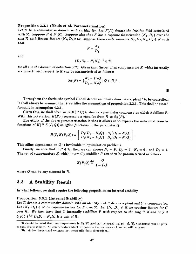
El

Proposition 3.2.1 (Youla et al. Parameterization)Let 1Z be a commutative domain with an identity. Let F(1R) denote the fraction field associatedwith R. Suppose F E F(1R). Suppose also that F has a coprime factorization (N1 , D1 ) over thering R with Bezout factors (Nk, Dk); i.e. suppose there exists elements N1 , D1 , Nk, Dk E 1Z suchthat

ND1

and(D1 Dk - NfN)-' E 1Z

for all s in the domain of definition of R. Given this, the set of all compensators K which internallystabilize F with respect to 1Z can be parameterized as follows:

SR(F) = Nk- DQ I Q E I.Dk - N 1 Q

Throughout the thesis, the symbol P shall denote an infinite dimensional plant 2 to be controlled.It shall always be assumed that P satisfies the assumptions of proposition 3.2.1. This shall be statedformally in assumption 4.2.1.

Given this, we shall often write K(P, Q) to denote a particular compensator which stabilizes P.With this notatation, K(P, -) represents a bijection from R to Sg(P).

The utility of the above parameterization is that it allows us to express the individual transferfunctions of H(P, K(P, Q)) as affine functions in the parameter Q:

H (P, K(P, Q)) = Dp(Dk - NpQ) Np(Dk - NQ)Dp(Nk - DpQ) Dp(Dk - NQ)

This affine dependence on Q is invaluable in optimization problems.Finally, we note that if P E "R, then we can choose N, = P, Dp = 1 ,Nk = 0 , and Dk= 1.

The set of compensators K which internally stabilize P can then be parameterized as follows

def -QK(P, Q)= 1-PQI

where Q can be any element in R.

3.3 A Stability Result

In what follows, we shall require the following proposition on internal stability.

Proposition 3.3.1 (Internal Stability)Let R denote a commutative domain with an identity. Let F denote a plant and C a compensator.Let (N, Df) E R be coprime factors for F over R. Let (Nc, De) C R be coprime factors for Cover R. We then have that C internally stabilizes F with respect to the ring 1? if and only if

6(F,C) =' DiDe - NNe is a unit of R.

'It should be noted that the compensators in Sx(F) need not be causal [17, pp. 3]. [?). Conditions will be givenso that this is avoided. All compensators which we construct in the thesis, of course, will be causal.

2By infinite dimensional we mean not necessarily finite dimensional.

El

NProof The proof in [56, pp. 45-46, lemma 4] applies to our general ring 1?. The main ideas arenow given.

If 6 is a unit in 7?, then the associated closed loop transfer function matrix

H(F, C)= D De NS Dc 1

D Ne D1 De 6has all of its transfer functions in R; i.e. H(F, C) E M(R). This proves one direction.

If H(F, C) E M(R), then we have

[ f Dc Nc ]E M(R).

The coprimeness of (NS, Df) and (Ne, Dc) then implies that j E 7?. This proves the other directionand hence completes the proof.

3.4 The Corona Theorem

We begin this section with an instructive example.

Example 3.4.1 (?1X as a Ring)The function space X"t is a commutative domain with an identity [56]. It shall be used throughoutthe thesis to define stability; i.e. it will be the the only ring over which we will work.

Moreover, we shall always assume that our plant P belongs to the fraction field associated withX"O. We shall also assume that it has a coprime factorization over the ring 3. With this assumption,we will be able to use the parameterization in proposition 3.2.1. This, in turn, will allow us toexpress system transfer functions as affine functions with respect to the parameter Q.

When we deal with the ring H we are implicitly concerned with 2 - finite gain stability asdefined in [11].

Given this, the following proposition will allow us to determine whether or not two functionsin X" are coprime.

Proposition 3.4.1 (Corona Theorem)Given N, D E 7? where R is X", then N and D are coprime in R if and only if

inf IN(s)| + ID(s)I > 0.3EC+

This proposition can be found in [56, pp. 341-342]. It is sometimes referred to as the CoronaTheorem. Loosely speaking, it says that N and D are coprime in 1? if and only if they have nocommon open right half plane zeros.

"It should be noted that not all functions in the fraction field of A have coprime factorizations [56]. In contrast,all stabilizable functions in the fraction field of 7* have coprime factorizations [52]. This shall receive furtherconsideration in the sequel.

3.5 Summary

In this chapter we presented various results from the algebraic systems literature. We are nowready to precisely state what fundamental problems shall be addressed in this thesis.

Chapter 4

Statement of Fundamental Problems

4.1 Introduction

In this chapter we precisely define what we shall refer to as the K-Norm Approximate/DesignJ-Problem. This problem shall be the focal point of the thesis. This problem addresses the ques-tions: What is a "good" plant approximant? How do we obtain a near-optimal finite dimensionalcompensator?

We also define two additional problems, the K-Norm Purely Finite Dimensional J-Problem andthe K-Norm Loop Convergence J-Problem. The first problem addresses the computation of optimalperformance measures using finite dimensional techniques. The latter, examines the convergenceproperties of designs which result from the Approzimate/Design approach taken in this thesis.

4.2 Basic Assumptions & Notation

In this section we shall make assumptions which will allow us to use the algebraic system-theoreticresults of Chapter 3. In doing so we shall establish notation to be used throughout the thesis.

Let P(s) denote the transfer function of a continuous time scalar infinite dimensional plant 1.Also, let {Pn(s)} 1 denote a sequence of finite dimensional (real-rational) approximants of P. Thesense in which Pn approximates P shall be stated in the sequel.

Throughout the thesis we shall assume that the plant P and the approximants Pn satisfy theassumptions in proposition 3.2.1. More precisely, we make the following assumption.

Assumption 4.2.1 (Permissible Plants and Approximants)Let F(R) denote the fraction field of a commutative domain 2 R with an identity (e.g. h"o). LetFe(R) denote those elements of F(R) which are expressible as the ratio of coprime factors in R.It shall be assumed that the plant P and the approximants {Pn(s)}'o are elements of Fe(R).

Given this, P has a coprime factorization over the ring R; i.e. there exists elements N,, D,, Nk, Dk ER such that

P = -- ?D,

'By infinite dimensional we inean not necessarily finite dimensional. Although not, explicitly stated. causality andlinear time invariance are implied.

2A domain is a ring such that the product of non-zero elements is non-zero.

andDDk - NpNk = 1

for all s in the domain of definition of R. It then follows from proposition 3.2.1 that the set of allcompensators K which internally stabilize P with respect to the ring R can be parameterized asfollows:

K(P,Q) = Nk - DPQDk - NQ

where Q E R. Given this, K(P, .) is a bijection from R to the set of all compensators SIZ(P) whichinternally stabilize P with respect to R.

Also, assumption 4.2.1 allows us to associate with each P, the elements N,,, D,,, Nk., Dk, E 7?where

Pn = N''Dn

andD,,Dk, - NpNk, = 1

for all s in the domain of definition of R. Again, from proposition 3.2.1, it follows that the set of allcompensators Kn which internally stabilize Pn with respect to 7? can be parameterized as follows:

K(Pn, Q) = Nk, - D,,QDk, - N,,Q

where Q E R.

4.3 A/-Norm Approximate/Design J-Problem

In this section we precisely define the /-Norm Approzimate/Design J-Problem. First, we shallneed some assumptions and definitions.

Given the discussion in the previous section, we let JA((., K(.,-)): Fe(R) x Fe(7) x R -+ R+denote a performance measure. We shall refer to it as the K-norm J-measure. This terminologyis used since in the sequel, K will denote the norm on one of the function spaces (X**, XJ2 ) and Jwill be represent either a sensitivity criterion or a mized-sensitivity criterion.

Given this, the optimal performance for the infinite dimensional plant P with respect to theK-norm J-measure shall be defined as follows.

Definition 4.3.1 (Optimal Performance)

defppt infJg(P, K(P, Q)).QEIZ

The optimal 3 solution to this problem shall be denoted Qpt. The corresponding compensatorwill be denoted Kpt and is given by

def Nk -D~pKopt = K(P, Qp ) = Nk - DQoptD - NQ 0 it

ahIi may be that an optimal solution does not exist. This technical point is nmot important at tihe moment.

As stated earlier, our primary motive is that of finding a near-optimal finite dimensional com-pensator for the infinite dimensional plant P. To do so, one starts by examining the optimizationproblem defined in definition 4.3.1.

In general, definition 4.3.1 defines an infinite dimensional optimization problem which is verydifficult to solve. The basic philosophy of this research endeavour has been to avoid the De-sign/Approximate approach which appears in the literature. In this approach, one first needs tosolve the above infinite dimensional problem for an infinite dimensional compensator. Then, oneapproximates the resulting infinite dimensional compensator to get a desirable near-optimal fi-nite dimensional compensator [14]-[16], [40]-[41]. Rather than this approach, we have taken anApproximate/Design approach.

In our Approximate/Design approach, we first "approximate" the plant P with a sequence of fi-nite dimensional approximants {Pn}*1 . Then, to obtain a suitable finite dimensional compensator,we consider the following finite dimensional optimization problem.

Definition 4.3.2 (Expected Performance)

pn te inf Jg(P, K(P., Q)).QEIZ

In the context of this work, we shall refer to pn as the expected performance. This terminology forpn is motivated by the fact that the numbers pin are typically used to guide us during the designprocess.

Let Q, denote the optimal 4 solution for the problem in definition 5.5.1. In accordance withassumption 4.2.1, Q, generates an internally stabilizing 5 compensator K, for P. This compensatoris given by:

Kn = K(P,,Q) = N ,- DDk, - NnQn

It is shown in section 6.3 that, in general K, need not stabilize P, even when Pn is "close" toP in the uniform topology on 1? 6. Consequently Kn, in general, cannot be placed in a feedbackloop with the infinite dimensional plant P. It is thus appropriate to ask whether or not K, canbe modified to obtain a near-optimal finite dimensional compensator for P. We shall see that fora large class of problems, the answer to this question is affirmative.

Toward this end, we define a "roll-off operator"

r: Q, -- Q

which maps Q, to Qn E 1?. From the above discussion, it is clear that the roll-off operator r mustbe chosen intelligently (see section 6.3). The exact form of r will be determined shortly.

Given this, we then consider the feedback system in Figure 4.1, obtained by substituting thefinite dimensional compensator generated by Qn, namely

- def - Nk,. - D~.Q,.Kn = K(PnQn) = N - D,,Qn

Dk, - NQ

"It may be that an optimal solution does not exist. Again, this technical point is not important at the moment.5We note that this may not be the case since Q. may not lie in the ring R. This point. is also associated with

existence issues and is not critical at the moment.6Since we shall be working over the ring 7", it is clear what is met by the uniform topology.

into a closed loop system with the infinite dimensional plant P. We note that although k, internallystabilizes P, it need not internally stabilize P. This critical issue will be addressed in the sequel.

Let H(P, k,) denote the resulting closed loop transfer function matrix from r, d to e, u. Wethen have

e H(P, kn) ,

where

1-PR, 1-PR,

Substituting for k, then gives

H(P, kn(On)) = D,(Dk - N,,Qn) N,(Dk, - N,,Qn)Dp(Nk, - D,,Qn) Dp(Dk, - NQn) 6(P, kn(Qn))

where

6(P, kn(Qn)) t= DP(Dk, - N,,Qn) - NP(Nk, - D,,Qn).

Assuming internal stability can be shown, we then have the following "natural" definition forthe actual performance.

Definition 4.3.3 (Actual Performance)

-def, = JW(P, K,)-

U

Comment 4.3.1 (Internal Stability)Adef-

Since _- Nk, - D,,QnDk, - N,,Qn internally stabilizes Pn, the factors Nk, - D,,Qn andDk, - N,,Qn must be coprime. This follows from proposition 3.3.1. Given this, it follows fromthe same proposition, that kn(Qn) internally stabilizes P if and only if 1 E R. This

O(P,R,(O,))argument will be used in the sequel.

Given the above discussion, we define the K-Norm Approximate/Design J-Problem as follows.

Problem 4.3.1 (Approximate/Design Problem)Find conditions on the approximants {P},*1 and on the roll-off operator r such that

lim ftn = popt.n--+oo

If a set of approximants {Pn}** 1 satisfy the above condition, then we shall say that the ap-proximants are "good"; i.e. a set of approximants {P}o_1 are good if they allow us to satisfy thecontrol objective. In this sense then, the K-Norm Approximate/Design J-Problem addresses thequestion: What is a "good" finite dimensional approximant?

1 0pt J (P Kopt)

/-Ln=J(Fn,Kn)

an= J(P Kn)

Figure 4.1: Visualization of Approximate/Design Methodology

Assuming k, internally stabilizes P, we have

Popt An.

This is because popt is the optimal performance. Given this, we would like to show that

lim n <_ pti.

Doing so, however, is equivalent to finding an internally stabilizing finite dimensional compensatorKn such that

Tin 5 PL0 t +E

where e > 0 is a given (apriori) optimality tolerance. In this sense, the K-Norm Approxi-mate/Design J-Problem is equivalent to that of finding a near-optimal finite dimensional com-pensator for the infinite dimensional plant P.

This K-Norm Approximate/Design J-Problem shall be the focal point of the thesis. Morespecifically, the problem shall be solved in the sequel for two distinct performance measures Jg.To define these measures we shall need weighting functions W, W1, W2 E R.

Let K denote one of the function spaces H** and H2. Suppose that F, G E F,(R) and Q E R.If the performance measure J has the form

def WJg(F, K(G, Q)) = ,1 - FK(G, Q) yV

then problem 4.3.1 will be referred to as an K-Norm Approximate/Design Sensitivity Problem. Asolution to this problem shall be presented in Chapter 6 when the norm||-||g is the X**o-norm. TheX2-norm case is addressed in Chapter 8.

If the performance measure Jg has the form

[W1def W2FK(G, Q)Jg(F, K(G, Q)) 1-FK(GQ)

oriW1

Q)def WV2K(G, Q)Jg(F, K(G, Q)) = ,1 - FK(G, Q)

then problem 4.3.1 will be referred to as an K-Norm Approximate/Design Mixed-Sensitivity Prob-lem. A solution to this problem shall be presented in Chapter 7 when the norm ||-||g is theH**-norm. The X2 -norm case is addressed in Chapter 8.

The above Approximate/Design problems are difficult for several reasons. These reasons arediscussed in section 6.3.

4.4 K-Norm Purely Finite Dimensional J-Problem

In practice we would like to be able to compute popt using finite dimensional algorithms. For theabove sensitivity/mixed-sensitivity criteria, the literature has typically considered infinite dimen-sional eigenvalue/eigenfunction problems in order to compute popt [14, pp. 28-31], [63, pp. 308].With an ultimate intention of providing purely finite dimensional techniques for computing pot,we shall also consider the following "purely" finite dimensional problem.

El

Problem 4.4.1 (Purely Finite Dimensional Problem)Find conditions on the approximants {Pn}oo such that

lim pn = p4opt.

In the context of this work, we shall refer to this problem as the K-Norm Purely Finite DimensionalJ-Problem.

This problem inherently addresses the question of computing the optimal performance p, usingfinite dimensional techniques.

Again, if Jg is a sensitivity criterion then we will refer to this problem as the K-Norm PurelyFinite Dimensional Sensitivity Problem. Analogously, if JA( is a mixed-sensitivity criterion thenwe will refer to this problem as the K-Norm Purely Finite Dimensional Mixed-Sensitivity Problem.These problems shall also be addressed in Chapters 6 and 7 for w* criteria. Chapter 8 shall addressthe problem for the case of an 7j2 performance criteria.

4.5 KN-Norm Loop Convergence J-Problem

Having the actual performance fin and expected performance pn converge to the optimal performancepopt is quite desirable. However, given this it is still very important to understand in what sensethe transfer functions associated with the actual system (P, kn) converge to those of the optimalsystem (P, Kt). Given this, we define the K-Norm Loop Convergence J-Problem as follows.

Problem 4.5.1 (Loop Convergence Problem)Given that limno An = pt and limn_.o pn = popt, in what sense, if any, do the transfer functionsassociated with the (P, kn)-loop converge to those of the optimal (P, Kopt)-loop ?

UIn this problem we concern ourselves primarily with the convergence properties of designs whichresult from the Approximate/Design approach taken in this thesis.

This problem shall be addressed in the sequel for each of the afforementioned design criteria.

4.6 Summary

In this chapter three problems were defined: (1) The K-Norm Approximate/Design J-Problem,(2) The K-Norm Purely Finite Dimensional J-Problem, and (3) The K-Norm Loop ConvergenceJ-Problem.

In the sequel we shall address each of these problems for R"* and R 2 sensitivity and mixed-sensitivity design criteria.

Chapter 5

HOO Model Matching Problem

5.1 Introduction

In this chapter we define the R** Model Matching Problem. It is shown how near-optimal real-rational solutions can be constructed for this problem by considering sequences of appropriatelyformulated finite dimensional model matching problems. The constructions presented shall beheavily exploited in subsequent chapters on design via N* optimization.

5.2 Infinite Dimensional HiX Model Matching Problem

In subsequent chapters, we will be examining optimization problems which have the followingstructure.

Definition 5.2.1def

pt inf |IT, - T2QIIQENjO

where T1, T2 E R .Given this, the R** Model Matching Problem is that of finding a near-optimal Q-parameter in

1.o.

I

Since T2 E ?* , we know from proposition 2.7.6 that it possesses an inner-outer factorizationover X**. We will denote this factorization by T2 = T2iT2., where T2, is inner in H** and T2, isouter in h**. This factorization shall be exploited throughout the chapter.

Throughout this chapter, the following technical assumption shall be made on T, and T2.

Assumption 5.2.1 (T1 and T2)(1) T1 E Ce 1.(2) T2, has a finite number of zeros on the extended imaginary axis; each with finite algebraicmultiplicity. See comment 5.2.1 below.(3) If T2. is not invertible in R*, then we assume that T2. E Ce.

1Functions in Ce are continuous everywhere on the extended imaginary axis.

The following comment establishes notation regarding the imaginary zeros of T2.. It also clarifieswhat we mean by each zero having finite algebraic multiplicity.

Comment 5.2.1 (Imaginary Zeros of T24: Finite Algebraic Multiplicity)We shall denote the zeros of T2. on the extended imaginary axis by the finite sequence {Wk} =0 . Itshall be assumed that the sequence is increasing and that its elements are distinct, non-negative,extended real numbers. We shall also adopt the convention that WO = 0 and w1 = oo. Given this,{wk} ~1 will denote finite zeros of T2. on the positive imaginary axis. {-wk} ~1 will denote finitezeros of T2. on the negative imaginary axis.

By assumption 5.2.1, each Wk has finite algebraic multiplicity. This multiplicity shall be denotedmk, is non-negative, and is generally a fraction.

Since T2, E Ce, we know that it is bounded away from zero on all closed frequency intervals notcontaining an imaginary zero. Consequently, if we define

d-1F(s) =m s"O ](s 2 + o2)"h

k=1

and

Ga(s) def ( a\s + a/

where a E R+, then

1TZ'(-) F(.) F-1(. + -) Ga(-), T 2.(.) F-'(.) G (.) E 'H* OfCeaa

for each a E R+.

Several points need to be made in order to emphasize the broad applicability of assumption5.2.1 above.

Comment 5.2.2 (Broad Applicability)

(1) T1 and T2 may be real-rational.

(2) T2j need not be continuous on the extended imaginary axis as assumed in [60]. It may, forexample, have a singular inner part; e.g. T2, = e~

(3) T2j may have an infinite Blaschke product [30, pp. 132]; e.g.

*I1-z~I s-zkT2;

k=1 -~k s+ 'k

where {zk}' are open right half plane zeros satisfying the Blaschke condition

Re(zk)

=1 + 2 Z

(4) The zeros of T2, on the extended imaginary axis, strictly speaking, may be branch pointsof T2. with respect to the entire complex plane; e.g. T2. = . In such a case we assume a

single-valued analytic branch in the open right half plane.

(5) T2 may possess removable singularities, poles, essential singularities, and branch points inthe open left half plane.

(6) Although T2, E Ce, this does not mean that T2 E Ce; e.g. T2 = e - ( ) (-).

(7) Although the outer function T2. = _, is not continuous on the extended imaginary

axis, it is admissible since it is invertible in R**; i.e. 1 - e-' E R**.

(8) Cases in which the associated Hankel operator rTrT2. is non-compact are permissible; e.g.

Ti= N, T2i = e~' (cf. proposition 2.9.2).

The above Model Matching Problem should be viewed as an inversion problem. This is becausein posing the problem we indirectly tell the mathematics to find an admissible Q which inverts asmuch of T2 as possible. The problem should thus be approached with an "inversion mentality".

In this section we shall construct a sequence {Q,} m =1 C ?o* such that given an optimalitytolerance e > 0, however small,

Po |IT 1 - T2Qm||u.i Yo + C

for m sufficiently large. This will allow us to obtain a near-optimal Q-parameter and thus providea solution to the NX** Model Matching Problem. To construct this sequence, we first shed light onexactly what part of T2 should be inverted.

From the above inner-outer factorization for T2, we immediately note that, in general, T2i isnot invertible in R**. We also note that any zeros which T2, may have on the imaginary axis, arealso non-invertible. This leads us to conjecture that we should invert T2, away from its imaginaryzeros in the closed right half plane. This statement/conjecture shall be formalized and confirmedshortly.

In order to gain insight into the i0* Model Matching Problem, one usually starts with someversion of the following proposition [23], [44, pp. 46]. The proposition emphasizes (and quantifies)the non-invertibility of T2i.

Proposition 5.2.1 (Inner Problem)Each of the following are equal:

inf || JT1 - T2i Z||h.(1ZEN**

rTrT (2)

Moreover, there exists Z, E 7VO, not necessarily unique, which attains the infinum in the "inner

problem" defined by (1); i.e.

|IT1 - T2iZo| . = mn IT1 - T2iZ||o.

In the sequel, we shall refer to Zo as the "inner solution".

Proof The existence of an infimizer Z0 can be proved using standard weak* convergence ar u-ments [5, pp. 134-137), [35, pp. 128), [24, pp. 85 - 86). The fact that the infimum is FTTi; is

essentially a special case of Nehari's Theorem [38]. Elements of this proposition can also be foundin [1], [39], [46], [51]. U

Typically, one solves the "inner problem", defined in proposition 5.2.1, in order to get a handleon the the optimization problem defined in definition 5.2.1.

The following lemma gives us further insight about the W"* Model Matching Problem. Morespecifically, it gives us a lower bound on i, which supports our conjecture that we should invertT2., away from its imaginary zeros, in the closed right half plane.

Lemma 5.2.1 (Bounds on po)

max{|T1(joo)|, Max|1T1(jok)|, T,; }I p. :5 ||T1||u.

kProof To prove this, we begin by noting that

defpO inf lIT1 - T2Q||. < |IT1||l.

QE7W0

since 0 E RO. This proves the upper inequality in the lemma.To prove the lower inequality, it will suffice to show that each of the terms IT1(joo)I, maxk JT1 (iwk)|,

and JT1 TrT is a lower bound for po.

From the maximum modulus theorem for W** (proposition 2.7.2), it follows that |T1(joo)11Ti - T2QII. for any Q E 7-O*. It thus follows that

|T1(joo)| 5 pto.

Since T2(jwk) = 0 for each k, from proposition 2.7.2 we have maxk |T1(iwk)| |IT 1 - T20||u.for any Q E 1o**. It thus follows that

maxIT1(jwk)| 5 po.k

Since T2 0 7o* C R*, we have infzEneo |IT 1 - T2iZ||a. J |IT1 - T2iT2.QII. for each Q E Ro.This then implies that infzEnHo |IT, - T2iZ|lu. < po. By proposition 5.2.1 the left hand side of

this inequality equals 1PT1r, . We thus have

11 Tl T2; 1 (Lo.

Combining the above gives us the desired lower inequality:

max{JT1(joo)), maxlT1(jwk), TT1T2; } 0 j.

This completes the proof.

Comment 5.2.3 (Lower bound for p,, at oo)Note that if we were infimizing over H**, rather than HO*, then we would again have the inequality

IT,(joo)| I pi, if T2 were to roll-off.

We see that lemma 5.2.1 gives a lower bound on p, which depends on T2, and on the imaginaryzeros of T2.. This supports our conjecture that we should invert T2, away from its imaginary zeros,in the closed right half plane. We shall soon show that the above lower bound is actually equal topo. The lemma also shows that since T1 E '*, po will necessarily be finite.

Our interest in the "inner problem" will be to use its solution Zo to construct near-optimalsolutions for the 1** Model Matching Problem. The idea will be to appropriately modify ("roll-off") Ti-' Z0 so that the resulting function is admissible 2 and near-optimal. This modification shallbe carried out in two steps. Each step is now described.

Main Ideas: Construction of {Qm,n}.

The first step will be to construct a sequence {fm},=i C N-* to modify the "inner solution".By this we mean that fm will be such that

|IT 1 - T2iZofMIH. po + 2E

for M sufficiently large. The function fn, as we shall see, will contain all the essential informationabout the imaginary axis zeros of T2,. It will be small near each imaginary zero of T2, and it willapproximate unity elsewhere. To construct the function, we shall exploit the fact that T2, has afinite number of zeros on the extended imaginary axis. The phase properties of fm will be criticalin achieving the above inequality.

After constructing the sequence {fm}m* to modify the "inner solution", we shall construct aninverting sequence {gn}* C RNo for T2,. This terminology will be justified shortly. The sequencewill be such that

T2 1 gn Eand

lim |IT 2iZofM(1 - gn)|| oo = 0n-+oofor each M, n E Z+-

We then define a double sequence according to

def of nQm,n T 2 Zo fm gn.

This sequence will lie in X** for each m, n C Z+. Hence, it will be admissible.Finally, the above are combined with the following inequality

|IT 1 - T2QM,nIIoo < IT1 - T2;ZofMIIoo + IIT2ifM(1 -gn Joo,

to show that there exists M, N E Z+ such that

po jT 1 - T 2 QM,n hI. < po + 3

for all n > N.We thus see that, on the one hand, the sequence {f m}* 1 allows us to keep the essential infor-

mation contained in T2,. On the other hand, the sequence {gn}** allows us to invert that partof T2, which is not essential. The two sequence together shall implement our idea of invertng T2 ,away from its imaginary zeros, in the closed right half plane.

The following algebraic result will shed light on the construction of the sequence {f m }, 1 whichwill modify the inner solution.

2In, genieral, T2, 1 Z, will have poles on the extended imaginary axis.

Lemma 5.2.2 (Algebraic Result)Suppose T,Y, f E ' where If| |1H,. 5 1 and ||Y||1 ||T||x. It then follows that

IT + (Y - T)f12 [8=jW] < max{IT(jw)1 2,| I|Y||.} + 2||T| 12{211 - cosu I|+ Isine1 - 6 | +|I |}

(almost) everywhere on the extended imaginary axis.

Proof The proof of this lemma is purely algebraic and is given to accommodate the skeptical.

IT + (Y - T)f12[ 8 =j j = IT(1 - f) + yf|2

= T(1 - f)12 + T*(1 - f *)Yf + T(1 - f)Y*f* + |Yf| 2

= 1T|2(1 - f - f* + |f|2l) + T*Yf - T*Ylf| 2 + TY*.f* - TY*|f12 + |Yf| 2

= |T12(1 - 2|f|+ |f12) + 2|T |2|f| - |T| 2(f + f*) + T*Yf + TY*f* - |f|2(T*Y + TY*) + |Yf| 2

= |T| 2 (1- If1) 2+2|T| 2 f|(1 -cos)+T*Y(f -f*)+(T*Y+TY*)f*-2|TIYIf| 2 cos(ot-oy)+ |Yf| 2

= |T12(1 _ IfI)2 + 2|T| 2|f|(1 - cosf) + IYf 2 - 2|T||Y||f|2 cos(Ot - 0Y) + |TI IYIej(** -6)j2|f| sinG+2|TIY| cos(Ot - Oy)f e-jef

After expanding each complex exponential into real and imaginary components, one obtains

IT + (Y - T)f|2[8=ju] = IT12(l Ifl)2 + IYfI2 + 2|TIIYIIfI cos(Ot - O)(1 - IfI)

+2|T12 1fI(1 - cos 61) + 2|TI|Y|If I cos(6t - Oy)(cos6j - 1)

+2|TIIYIIf I sin(Ot - Oy)(sin6f - Of)

+2|TI IY|IfI sin(Ot - Gy)65

(almost) everywhere on the extended imaginary axis.Given this, let

defp max{|T(jw)|,||Y||lj}.

With this definition, and the fact that If||j. I 1, we then have

IT + (Y - T)f|2[8 =j] < A2(1 - 2|fl + If12 + If|2 + 2|fI - 21f 12)

+4p12 |1 - cos 1|+ 2pu2 Isin6f - OI + 2p2I8,Ior equivalently,

|T + (Y - T) f| 2[.3j] 2 +12 4 p2|1 - cos5I| + 2 p2 IsinOf - Of5 + 2y 2

(almost) everywhere on the extended imaginary axis.Since by assumption IIY|I. 5 ||TH., we have p < ||TH .. This, and the above inequality,

then gives us that

IT + (Y - T )f| 2[ < i2 + 2||T ||2 { 2|1 - cos0u| + |sin65 - Of + | 6I}

(almost) everywhere on the extended imaginary axis. This, however, is the desired result. U

Comment 5.2.4 (A Convexity Argument)If we let Of = 0 in the above lemma, we get f E [0, 1]. In such a case, the desired inequality followsfrom a simple convexity argument:

IT + (Y - T)fV I (1 - f)ITI + fIY| 5 max{ITI, IYI}.This simple case captures the essential ingredient needed to construct the sequence {fm}.=1. Thisis demonstrated in the following proposition.

Proposition 5.2.2 (Phase Result)Let {fm},' =1 denote a sequence of ?** functions such that

l|fmI||. 5 1for each m E Z+ and

lim IIm|, = 0.

Given this, there exists M 4! M(E, |IT1||N.) E Z+ (independent of w) such that

IT1 - T2iZofm[,=jI max{|T 1 (jw)|, IETTr 1} + E

for all m > M, (almost) everywhere on the extended imaginary axis.

Proof We begin by defining Ytf T1 - T2j Zo. This then gives

T1 -T 2iZofm = T1 + (Y - T1)fm.

From proposition 5.2.1, ||YII = Tr; . From lemma 5.2.1, T1rTr T IT1| |. Combiningthese gives |IYI||. 5 |IT1||,.,. Given this, from the algebraic result in lemma 5.2.2, it follows that

IT1 - T 2 iZofm|2 jw] = IT1 + (Y - Tl)fm| 2 w

S max{IT1(jW)| 2, lIyI|I.} + 2||T1I.{2|1 - cosO/mI + |sin/m - 6fm + +6fm|}(almost) everywhere on the extended imaginary axis. Substituting IIYII,. = L"Tr 1 1 into the firstterm then gives

|T1 - T2i Zofm| 2[M1 1 max{|T1(jw)|2,T1 r +2 |12

(almost) everywhere on the extended imaginary axis. From the assumed phase property of fm, itfollows that the last three terms can be made arbitrarily small, uniformly in frequency, by taking msufficiently large. More precisely, there exists M =e M(E, IT1 ||Ig..) E Z+ (independent of w) suchthat

IT1 - T2Zofm .j]5 max{IT1(jw)I, (ILTT; 1} + E

for all m > M, (almost) everywhere on the extended imaginary axis. This completes the proof. I

We emphasize that only magnitude and phase assumptions on fm were used to obtain theabove result. That such assumptions should suffice follows "intuitively" from the simple convexityargument given in comment 5.2.4.

In the proof of proposition 5.2.2 above, the phase assumption seemed indespensable. Thefollowing shows that it can sometimes be relaxed.

Comment 5.2.5 (Relaxing the Phase Assumption)It should be noted that if T1 (jw) = 0, then the phase assumption on fm becomes unnecessary.Although not transparent from the proofs given, it can be seen as follows. If fml 1 and TI(jw) =0, then we have

IT1 - T2jZofmI[=jW] = |YfmI[p=jw] |YI[p=jw] ||lluyII 5 IrT1T2 '

which proves the claim.

We now construct the sequence {fm},* . It will possess the properties needed to modify theinner solution Z0 , in the manner suggested earlier. To perform the construction, we exploit thefact that T2. has a finite number of zeros on the extended imaginary axis.

Proposition 5.2.3 (Sequence to Modify Inner Solution)There exists a sequence {fm}m=I C 'O of outer functions which possess the following properties:

(1) fn E Ce for each m E Z+.(2) ||fm|[u I 1 for each m E Z+-(3) The phase of f m can be made arbitrarily small, uniformly in frequency, by taking m suffi-

ciently large; i.e.

mim ||/m|| 1,C = 0.

(4) fm converges uniformly to unity on all compact frequency intervals excluding the points{wk} k; i.e. (see definition 2.10.5) for each 6 > 0, however small,

lim 1(1 - fm)XR/B(oo,6)UU' B(wA,6) O= 0.

(5) If m& > 0, then fm(±jWk) = 0 for each m E Z+-

ProofThe sequence defined by the following irrational function satisfies conditions (1)-(5) of the

proposition.

def a k "(m )a) +--1 2 ' 2 "'_L2S +-f s) ==1 S M k m

We note, in particular, that

2m

for some B E R+. We see that fm is irrational even when the mk are integers. We also note that

fm(s) = [F(s) F- '(s + 1) Gm(s) M

This completes the construction. U

Comment 5.2.6 (Phase is Critical)It should be emphasized that it is the phase property of f, that makes it a very special function.It is easy to construct rational sequences which satisfy the other properties in proposition 5.2.3;e.g. the sequence defined by

fm(s) c ( 1 (+m

However, finding a rational sequence which also possesses the special phase properties, at firstglance, seems very difficult. Since fm E C,, we know from proposition 2.10.1, that such a sequencecan be constructed.

We now use the sequence {fm},*OI from proposition 5.2.3, in conjunction with proposition 5.2.2,to obtain the following key theorem. To our knowledge, the key ideas behind the following theoremfirst appeared in [14, pp. 68-72].

Theorem 5.2.1 (Modifying the Inner Solution)Given that T1 E C. and that T2. has a finite number of zeros on the extended imaginary axis, thereexists M = M(e,T1) E Z+ such that

|IT 1 - T2iZofml 7 . po + 2E

for all m > M.

Proof To prove the theorem, we begin by defining

Y = T1 - T 2 Z.

This then gives

Ym T - T 2 1Zofm = T1 + (Y - T1)fm.

We shall examine the magnitude of this quantity on two sets. We denote these sets S6 and R/Sb.To prove the theorem we proceed in three steps. (1) First, we show that there exists a set Sb onwhich Im I satisfies the inequality for m sufficiently large. Here we exploit the continuity of T andthe magnitude and phase properties of fm (modulo proposition 5.2.3). (2) We then exploit themagnitude and compact convergence properties of fm to show that IYm I will satisfy the inequalityon R/S 6 for m sufficiently large. (3) Finally, we combine the results in steps (1) and (2).

Step 1: Analysis on S6.In this step we construct a set Sb such that

IYmXsI,1.oo po + 2E.

To do this we proceed as follows.

(a) Constructing Sb.

-Mffiawvn - no"

First consider the behavior of T1 near joo 3. By assumption 5.2.1, T1 is continuous everywhere ondefthe extended imaginary axis and hence at joo. It thus follows that there exists f? = II(e, T1 ) E R+

such that IT1(jw) - Ti(joo)| < E for all w such that wI ;> 0; i.e. for each w in B(oo, A) n(-oo, -fl) U (fl, oo). Hence

(T 1 - T1(joo))XB(o,A) KE. ''

This takes care of the point at oo. Without loss of generality, we can assume that the points{wk} o are finite.

Now consider the behavior of T1 near each point jWk 4. Since T is continuous at jw, it followsthat there exists 6k 45 6k(E, Ti) E R+ such that |TI(jW) - T1(jwk) < c for all w in B(Wk,6k)(-wk - 6k, -Wk + 6 k) U (wk - bk,Wk + 6k). Hence

(T - T1(jWk))XB(k,bk) 1 < f

for eack k. This takes care of each point Wk.We now define

6 =6(e, T1) = min{ ,mi n 6k}.

This quantity is well defined, and positive, since we are minimizing over a finite number of positiveobjects. This is because T2, has a finite number of zeros. Given this, it then follows that

(T - T1(joo))XB(oo,b) N < E

and

(T 1 - T1(iok))XB(wA,6 ) < E

for each k.We now define the set S6 as follows

Sb tf B(oo, 6) U U_ OB(Wk,6).

This set represents points which are "near" the points {oo, {wk}o}.

(b) Upperbound for T1 on S6.Here, we would like to obtain an upper bound for T1 on S6. From part (a), it follows that

T1XB(oo,6) [Pia5 |ITI(joo)I + J(T1 - T1(joo))XB(o,6) y 5 |T1(joo)i + E.

It also follows that

T1XB(wk,6)J :5 |T1(jw)J + (T 1 - T1(jwk))XB(w,s) 5T1(jW)| + E

for each k. Combining the above, then gives us

||T1Xs 6 Io 5 sup JT1XB(Z,6) < sup |T1(jz)| ±E.zE{oo,{wA}kO} zE{oo,{wA}Q0 }

3 Thie point -oo is treated analogously.4 The points -wk are treated analogously.

IiiiiiliC.= -

M"

This, however, is equivalent to

||T1Xs, 5ue. max{1T(joo),niax IT1(jwk), IrTlT;-}+e.

This gives us an upper bound for T1 on S6 . We emphasize that this upper bound was obtainedby exploiting the continuity of T1 and the fact that T2. only has a finite number of imaginary zeros.

(c) Inequality on S6.From proposition 5.2.3, we know that there exists M1 = Mi(e, T1 ) E Z+ (independent of w)

such that

IYmgIB.j] max{|T1(jw)|, Tr, } + E

for all m> M1 . In obtaining this, we have exploited the magnitude and phase properties of fm.Since M1 is independent of w, the inequality holds (almost) everywhere in S6. Given this, we

obtain ||YmXs, 1,,. 5 max{IITXsII., rTrT I} + e for all m> M1 .Combining this inequality, with the upper bound obtained above for T1 on S6, gives IYXsllwoo <

max{IT1(joo)I, max ITi(jk)|1, I } + 2e for all m > M1 .

From lemma 5.2.1, we have max{IT1(joo)|, maxk IT(jwk)|, rT1r; } p. Given this, we thenhave

||Ym X Is,|| : y. + 2e

for all m > M1. This completes the analysis on S6. We now turn to R/S 6 .

Step 2: Analysis on R/S 6.

We now consider the set R/S 6 =- R/B(oo,6) U U1.=B(wk,b). On this set, for each m E Z+ wehave

Ym XR, = (Yfm + T1(1 - fm))XR/S, o fm 1 (1- fm)XR/s 6

Since |Ifm ||I,, 1 for each m E Z+, by proposition 5.2.3, this becomes

YmXR/S, III 0 0 1Yu7 + IIT1 I,1 (1 - fm)XR/S

for each m E Z+By proposition 5.2.3, the second term can be made arbitrarily small ( 2e) by taking m suf-

ficiently large. How large m needs to be, depends on e, on ||T 1||,., on 6(eT 1 ), and on f(ET).

Consequently, there exists M 2 tf M 2 (E, T1) C Z+ such that

YmXR/S IIYIIuoo + 2e

for all m > M 2. In obtaining this, we have exploited the magnitude and compact convergenceproperties of fm.

From proposition 5.2.1, ||Y|7 = -PTT . From lemma 5.2.1 we have 1Tr p/. Giventhis, we then have

YmXR/S, o - ZE

for all m > M 2. This completes the analysis on R/S 6 .

Step 3: Combining steps (1) and (2).

Combining the results of (1) and (2) assures the existence of an integer M d' M(e T1) cf

max{M1, M 2} E Z+, such that

||Ym1 7.| po + 2E

for all m > M. This completes the proof.

Comment 5.2.7 (Sifting Property of fm)Upon inspection of the above proof, we see that

IT1 + (Y - T1)fm||17j 5 max{ IT1(joo)|, maxT1(jok)|, ||YI|y } + 2e

for m sufficiently large. This sifting property of fm, we emphasize, is mainly attributed to themagnitude and phase properties of fm. Of course, the continuity of T1 is also important.

As we shall see, theorem 5.2.1 above and theorem 5.2.2 below are at the heart of the X"i resultspresented in the thesis. Together they will show how one can modify the Z, to the "inner problem"considered in proposition 5.2.1, in order to construct nearly-optimal solutions to the X" ModelMatching Problem defined in definition 5.2.1.

We now construct the sequence {gn}** 1. To do so, we exploit the fact the zero structure of T2.on the extended imaginary axis.

Proposition 5.2.4 (Inverting Sequence for T2. )There exists a sequence {gn}*=1 C .o of outer functions which possess the following properties:

(1) {gn"}, is uniformly bounded in ?V0.(2) Tij g- , T2 .g-1 e V n Ce for each n E Z+.

(3) gn uniformly approximates unity everywhere except on open neighborhoods of the points{jwk} 0k=; i.e. (see definition 2.10.4) for each 6 > 0,

lim (1- gn)XR/UlOB(w,5) = 0.fl4o kOk 00o

(4) g'g n E H**, n Ce for each m,n Z+.

(5) If mk > 0, then gn(wk) = 0 for each n E Z+.

We refer to {gnl'" as an inverting sequence for T20.

Proof The sequence defined by the function

__mo _1 ( mkdef 3 32 +w mn

gn (s) = 1± 1

satisfies the conditions of the proposition. We emphasize that gn is, in general, irrational since theMk, in general, are fractions. We also note that the sequence {gn}' 1 constructed above is the

same inverting sequence that we would use if T2. were real-rational. Finally, it should be notedthat

1gn(s) = F(s) F-'(a + -) Gn(s).n

This completes the construction.

Example 5.2.1 (Sample Functions: T20 and gn)The following indicate that proposition 5.2.4 covers a large class of outer functions T20.

(a) If 2. = choose gn = .

(b) If T20 = f choose g = .

(c) If T2. = Q choose gn .

(d) More complicated outer functions may require the use of [24, pp. 85; theorem 7.4] toconstruct gn. The results in [17] may also prove useful.

U

Combining the previous theorem and propositions leads us to the following key theorem.

Theorem 5.2.2 (Near-Optimal Irrational Solution)Let

defQm,n - Qofmgn

where Q0 =e T 2. jZo. Then, Qm,n E Ho for each mn E Z+. Also, for each m,n E Z+, wehave Qm,n( jWk) = 0 for each k = 0,1,. .. ,l. Moreover, there exists M =e M(E,T1) E Z+ and

N =f N(E, M) E Z+ such that

po |T1 - T2QM,n||Ii. po + 3

for all n > N.

Finally, from the integer valued functions defined by M(E, T1) and N(E, M), it follows that wecan construct a sequence {Qm}m=1 such that

(1) Qm E H' for each m E Z+

(2) If mk > 0, then Qm (jWk) = 0 for each m E Z+-

(3) po < |IT1 - T2Qm||joo < po + 3 for all m > M(E, T1).

ProofThe proof will proceed in three steps.

Step 1: Admissibility of Qm,,,.

We have

Qm,n 4= T2o'Zofmgn.

By proposition 5.2.3, fm E N* for each m E Z+. By proposition 5.2.4, T2 j~Ign E H** for eachn E Z+- Combining these gives us that Qm ,n E N* for each m, n E Z+-

By proposition 5.2.3, fm(jok) = 0 for each m E Z+ and for each k = 1,2,.. .,l. SinceT -1gn E ?** for each n E Z+, it follows that it cannot have poles at the points jwk for any n. Thisimplies that it cannot cancel the imaginary zeros of fm for any m. Consequently, Qm,n(jo&k) = 0for each m, n E Z+ and for each k = 0, 1,.. .,l.

Step 2: Near-Optimality of QM,n.

(a) Main InequalityTo prove the rest of the theorem, we use the following inequality:

|IT 1 - T2Qm,nIIj. = |IT 1 - T2iZofmgnI|7j. ||T 1 - TiZofmI||j +| T2iZofm(1 - gn)||7..

(b) Use of fm to Modify Inner Solution.

From theorem 5.2.1, |IT 1 - T2jZofmII. IO + 2c for all m > M =e M(e, T1). Let m = M.This then gives

IT 1 - T2QM,nI 7 .o /o + 2E + 1IT2iZofM(1 - gn)||0.-

(c) Use of gn to Complete Inversion of T20 .From proposition 5.2.3, we have that fM C Rw and is zero and continuous at each point jik-

From proposition 5.2.4, gn uniformly approximates unity everywhere except on open neighborhoodsof the points {jw k}1 _; i.e. (see definition 2.10.4) for each 6 > 0,

lim 1(1 - gn )X R/UIn. (w;,,6) = 0.

From proposition 5.2.4, the g,, are uniformly bounded. Given this, it follows from lemma 2.10.1that we can make the last term in the above inequality arbitrarily small by taking n sufficiently

large. More precisely, there exists N t N(e, M) E Z+ such that

||T 2iZofM(1 - 9n1[o < E

for all n > N. This implies that

IT1 - T2QM,nllHI < yo + 3E.

for all n > N. This proves the first upper inequality. The lower inequality follows from the defini-tion of p0 and the fact that {QM,n}N 0 '

Step 3: Construction of Qm.The construction of the sequence {Qm}m"* follows from the above. This completes the proof. I

Theorems 5.2.1 and 5.2.2 show that under the very weak assumption 5.2.1, we can modifyany solution Zo of the "inner problem" to find a nearly-optimal Q-parameter for the R** ModelMatching Problem defined in definition 5.2.1. Moreover, in the proof of theorems 5.2.1 and 5.2.2we have indicated how such a Q-parameter can be constructed. The proofs show that to constructa near-optimal solution one needs to invert T2, away from its zeros in the closed right half plane.The following example serves to further illustrate the construction.

Example 5.2.2 (Sample Functions: T20, fm, and g,)

Suppose that T2, = (_I) (a2+1 a+4

1 1 11The sequence defined by the function fm ( 10m"( '8+1000) *-j+.OOOl \.) i +001 *.00satisfies the properties in proposition 5.2.3.

The sequence defined by the function g, = +-J1 (_ 2) ( satisfies theconditions in proposition 5.2.4.

Note:The sequences {fm}*1 and {gn},"O1 depend only on the zero structure of T2,. They do not notdepend on T 2,.

Although the construction presented in theorem 5.2.2 has been obtained under the weak as-sumption 5.2.1, the ideas cover a much broader class of T1 and T2. The following comment is metto illustrate this point.

Comment 5.2.8 (Form of Construction, Generality, Main Ideas)In summary, it has been shown that if there exists functions F and G, which satisfy the followingconditions

(1) T2 '(.) F(-) F-'(. + ') Ga(-) E 1*" for each a E Z+,

(2) lim_.o, F(-) F-1(. + ) Gm(-) K 1,

(3) lime_.o 6F(-) F-1(-+L) Gn(-) < B for some B E R+,

(4) The sequence {F(.) F- 1(. + 1) Gn(-)}L 1 approximates unity on all compact frequency in-tervals not including an imaginary zero of T24,

then a near-optimal solution to the X** Model Matching Problem can be constructed from thedouble sequence defined by the following function

Qm,n = T2 Zo fm gn

where

fm =[ F(s)F-1(s +±) Gm() m _

m S + m

and1gd= [ F(s) F-1(s + -)Gn(s) ]n

Such functions F and Ga were shown to exist under the weak assumption 5.2.1.The ideas which permitted the above construction shall be used extensively throughout the

thesis. We thus point out the "main ideas".

ru~__-~ _____________

In the construction we modify the "inner solution" Z, by "rolling it off" with f, as in proposition5.2.3. This really is the main step. It can be done primarily because of the special phase propertyof the irrational roll-off function fm.; i.e. the phase of f, can be made arbitrarily small, uniformlyin frequency, by taking m sufficiently large; i.e.

mlim ||6/m Ile = 0.

We then choose m = M sufficiently large. How large M must be chosen depends on e and T1.Finally, we show that given M, N can be chosen sufficently large so that

QM,N = T20 'ZofMgN(M)

is near-optimal. How large N must be depends on e and M. Here the main role of g, is to assurethe strict propriety of QM,N and to assure that it has no poles on the imaginary axis. It allows usto invert T2, in a stable manner.

Thus far we have only addressed the problem of constructing near-optimal solutions for the'H** Model Matching Problem defined in definition 5.2.1. We now address the computation of thequantity p.

5.3 Computation of po

Often it is necessary to determine y,. The following proposition indicates how one might, inpriciple, compute the value p,,. All assumptions made in the previous section are assumed to holdhere.

Proposition 5.3.1 Each of the following equal p,:

inf0 ||T1 - T2Q||u- (1)QEWO

inf |IT 1 - T2jQ||u. (2)11 EN**

{Q(jok)=O; k=0,1,...,l}

max{ IT1(joo)|, maxIT1(jwk)|, rTr } (3)

Proof The proof shall proceed as follows: (a) 2=3 (b) 1=3.

(a) (2=3)We claim that the key to proving proposition 5.3.1 is showing that (2=3); i.e.

inf |IT 1 - T2jQ||j =p

{Q(jwA)=O; k=0,1,---,1}

wherepmax{|T1(joo)|, max|T1(jok)|, rr .,

We know from proposition 5.2.1 that infzeioo |IT 1 - T2iZIJ|u = 07,T . Since the set of Q E X0which satisfy Q(jwk) = 0 for each k also lie in ?**, we have

||T = inf |IT 1 - T2 iZ||u < inf |IT 1 - T2iQII||W.r T, l Z E " Q E N 0

{Q(jwk)=O; k=0,1,...,}

From proposition 2.7.2 we have |Ti(joo)| |IT 1 - T2iQII. for each Q E R**, including thosewhich satisfy Q(jwk) = 0 for each k. Consequently,

IT1(joo) inf |IT 1 - T2iQI||uO.

{Q(jwk)=o; k=0,1,...,4}

For each Q E XH0* which satisfies Q(jok) = 0 for each k, proposition 2.7.2 gives us ITl(iwk)I <

|IT 1 - T2jQ||u. Consequently,

max|IT1(jok)| I inf ||T1 - T2iQ||Ieok QEng

{Q(jwk)=O; k=O,...,l}

Combining the above then gives

def= max{IT1(joo)I,maxlT(jwk)|,||YI|,o} < inf |IT 1 - T2iQ Ilu.

k QEnO{Q(iwk)=O; k=O,...,1}

To show that (2=3), we thus only need to prove the converse inequality. To prove the converseinequality, it suffices to construct a sequence {Zmm}*=1 C ** such that Zm(jok) = 0 for eachk = 0, 1,..., 1, and such that

|IT 1 - T2iZmI|o. 5 max{IT1(joo)I,maxIT1(Wk)|, JTr;} + 3e

for m sufficiently large. The existence of such a sequence, however, is guaranteed by theorem 5.2.1;just choose Zm = Zofm. This proves the converse inequality and hence that (2=3).

(b) (1=3)We now prove that (1=3); i.e.

defpo - inf ||T1 -T2QI||u. = P,

where againdef= max{|T(joo)I,max|T1(j ),iWk)IrT }

From lemma 5.2.1, we have that

P ! po.

To prove that (1=3) we need to prove the converse inequality. To do so it suffices to constructa sequence {Q mlm""= 1 C ROO such that

IT1 - T2Qm|Iu- max{IT1(joo)I, max| T1(jWk)|, F T }+3e

for m sufficiently large. The existence of such a sequence, however, is guaranteed by theorem 5.2.2;just choose Qm = T2 j'Zofmg, where m = M(E,T1) and n = N(E,T1) as defined in the theorem.

This proves the converse inequality and hence that (1=3).

Proposition 5.3.1 shows that

yo = max{ITi(joo)I, maxITi(jo)|, TPT 1 T2*-

Given this, we have the following corollary.

Corollary 5.3.1 (Spectral Result)If

max{IT1(joo)I, maxIT1(jwk)I} rTiT ,

then

YO = PT1 T2*; -

This result shows that if the assumption in corollary 5.3.1 is satisfied, then to compute pA allthat we need do is compute rT1T. ; the operator norm of the Hankel operator rTTr. This,

in general, involves solving an infinite-dimensional eigenvalue/eigenfunction problem [61]. Thiscomputation can be particularly difficult when the operator is not compact. In the sequel we willshow how this computation, in many cases (including the non-compact case), may be carried outby solving a sequence of finite-dimensional eigenvalue/eigenvector problems instead.

The following lemma is presented to show how one might construct T1 so that the assumptionof corollary 5.3.1 is satisfied.

Lemma 5.3.1 (Construction of T1 )Suppose that T71 E X1 B and satisfies

max{IT1(joo)|, maxIT1(jwk)|} = inf ITi(jw)I.k wERe

Also, let z be any point in the extended open right half plane, such that T2 (z) = 0. We then have

max{IT1(joo)I,max|T1(jok)|} T2

Proof From proposition 5.2.1, there exists Zo E 1* such that

T lI, T1 - T2 ZoIIw-

From proposition 2.7.2, we have

2 IT1(z)lSince Tj' E XIB, the minimum modulus theorem [50, pp. 159] can be applied to get

> inf |T1(jo)|.WER,

The result then follows since the right hand side equals max{IT1(joo)|, maxk |T1(jwk)I} by con-struction.

This lemma can be applied to T2j = e-8, for example.

5.4 Computation of Hankel Norm

The difficulty in computing p, can be attributed to the difficulty in computing the Hankel normrTTi . This computation typically requires that one solve an infinite dimensional eigenvalue/eigenfunction

problem [14, pp. 28-31], [61], [63, pp. 308]. In this section, it is shown how the computation canbe carried out by solving a sequence of finite dimensional eigenvalue/eigenvector problems.

Throughout this section we assume that {T 1.} 1,{T 2,n}0* C RX"O, where T2,, is inner in1" for all n E Z+. We begin with the following proposition. Loosely speaking, it shows that

ITi1 is lower-semicontinuous in T2 in the compact topology on H".

Proposition 5.4.1 ("Lower-sernicontinuity" Hankel Result)Suppose that

liM |iTI - T1||I = 0and

lim1 (T 2n - T 2j)X[-n,O = 0

for each 0 E R+, however large. It then follows that

Trr T lim rT, .

Proof Let v E C2 be such that 1v1LC2 = 1 and

rTJ; TT 2 . Vr 2 +E.

Given this, it follows that

11rTS 1: 1T(2 -Tni +2.)s£j2 + E < 1rT, (T 2 jT 2 ni).V £C2 + PT1 T2*ivC~T1 T; PT(T 2-T.+Ta2 )*V( +£2 7-v ~r

< 1T1(T2 -T2i )*vI + TT* V 1, + .

Since v is not necessarily a "maximal vector" for LTT; , it follows that

1T2 1 T1(T2 -T2)*Vf + ITT I + E

From lemma 2.10.2 and our assumption on T2 ., it follows that the first term can be made arbitrarily

small by taking n sufficiently large. Consequently, there exists N t N(E, T1, v) such that

11TT* T2.- 11: T 1 T2n I± 2,E

for all n > N. We also have

r T,T* - T ; + T :5 r T T; + ||T1 - T16||0.

Combining this inequality with the previous, gives the result. U

Since T1 E C,, we know from proposition 2.10.1 that there exists a sequence of RH" functions{T 1.}'* 1 which uniformly approximate T1 . Given this proposition, we have the following theoremwhich gives insight into the computation of T1 T 2, ..

Theorem 5.4.1 (Spectral Result: Computation of Hankel Norms)Given that

lim ||TI, - T1 ||%. = 0,fl--+0

each of the following imply that limn_.o rT1 ,; = rTT .

lim T2n. - T2 =0 (1)n--+oo '7.to0

lim T1(T 2n. - TO2) 0 (2)n--+oo 7joo

T1(joo) = 0; lim (T 2 n. - T2i)X[-n,O] = 0 (3)

|Ti(joo)| TTrT.; lim (T2 - T2i)X[O,O] = 0 (4)

for each fl G R+, however large.

IProof The proof of (1) - (3) follows from the following inequality

T1,T - IrT1T2. |5 T1lTn -T1T-

< Ir(T -T)T* T(Tn -T') ||T1 T1||Io. + I T1(T 2 . - T2 ) -

To prove (4), we invoke proposition 5.4.1 to obtain

'T1T* K lim T1 2Tnj

This proves one direction. To prove the other direction we proceed as follows. Let Q0 E ?10 besuch that

IT, - T2jQ11ue max{ |T1(joo)|, rTr }T +.

The existence of such a Q0 is guaranteed by theorem 5.2.1. Given this, we have

rTnT = 1 T1, - T2 i Z :o 1 T1, - T2ni Qo

|IT1 - T2 Q0||u. + |IT1, - T1I| 7 o + (T2i - T2 . )Qo

< max{ IT(joo)l, rTrT; } + E + ||T1, - T1%. + I(T 2i - T2, )QO -

By assumption, IT,(joo)| I r T . Hence, the above inequality becomes

L'T1 T; 1 ; E + IT1, - T1|II + (T21 - T2,.)Qo

The second norm can be made arbitrarily small by taking n sufficiently large. This followsby our assumption that TI, approximates T, uniformly. By lemma 2.10.1, the last term can be

76

made arbitrarily small by taking n sufficiently large. This is because T2,,. is uniformly bounded,it approximates T2, on compact frequency intervals, and Q, rolls-off. Consequently, there exists

N = N(e, Q,) E Z+ such that

rT 1 T2 T P1rT;T2 + 3E

for all n > N. This proves the other direction and completes the proof. I

Comment 5.4.1 (Applicability, Spectral Implications)We note that the criterion in (1) is a continuity statement. It implies that T, 1; is continuousin T2, when T1i uniformly approximates T1 . Since RR"0 is not dense in N**, the criterion in (1) isusually not applicable; e.g. T2, = e-' cannot be approximated uniformly by RX"'> functions.

The criteria in (2) and (3) are helpful only when T1 rolls-off.

Unlike the other criterion, the criterion in (4) is usually applicable. It applies to cases in whichthe Hankel operator ITT2; is non-compact; e.g. T1 E RX** proper and T2, = e-' (cf. proposition

2.9.2). In such cases, the non-compact Hankel operator cannot be approximated by finite rankoperators. Moreover, it is not clear to us how one would approximate a non-compact Hankeloperator 5 . It also applies in instances where T2j has an infinite number of poles and/or zeros;e.g. an infinite Blaschke product. To verify the inequality criterion in (4), lemma 5.3.1 may provehelpful. If oo is an essential singularity of T2j, then the inequality is automatically satisfied. Thishas been shown in [61].

Finally, the spectral implications of theorem 5.4.1 must be acknowlegded. More specifically, wereiterate that computing 'Tr 1 amounts to solving an infinite dimensional eigenvalue/eigenfunctionproblem [14, pp. 28-31], [61], [63, pp. 308]. Theorem 5.4.1 gives weak conditions under which sucha computation can be carried out by solving a sequence of finite dimensional eigenvalue-eigenvectorproblems [23]. Since computing the above Hankel norm is crucial in many X** design procedures,this theorem is extremely useful.

U

5.5 Sequences of Finite Dimensional 70 Model Matching Prob-lems

The R** Model Matching Problem, in general, defines an infinite dimensional optimization problem.Obtaining a solution is often difficult and requires sophisticated mathematics 6. It is thus naturalto ask whether or not solving a sequence of appropriately formulated finite dimensional problemscan yield desirable results. Solving a finite dimensional Ri0* Model Matching Problem requires littlemathematical sophistication. Also, much software exists to support such an approach.

Let {T1.}*_1 and {T 2 .}**n be sequences of RX** functions. Consider the finite dimensionalR** Model Matching Problem defined by the following optimization problem.

Definition 5.5.1.n = inf ||T1. - T2nQ|I

QERWiO

'Distribution theory may be helpful in answering this question.6 Computing Z0 may be difficult.

Our goal is to gain insight into the infinite dimensional problem defined in definition 5.2.1, bystudying the finite dimensional model matching problem posed in definition 5.5.1. This, of course,is reasonable only if T1, and T2, approximate T1 and T2, in some sense. We thus make additionalassumptions on the sequences {T 1,}** 1 and {T2n}*1

Assumption 5.5.1 (T1 , Approximates T1 Uniformly)Throughout the section, it shall be assumed that the sequence {TI,}** 1 satisfies

lirM |T1, - T1||I = 0.n-.#oo

Since T1 E Ce, we know from proposition 2.10.1 that it can be uniformly approximated by R1**functions. Hence, this assumption is justified.

As with the X** Model Matching Problem, the above finite dimensional model matching problemmust be approached with an inversion mentality. Given this, it should be clear, for example, thatwe will need to invert the outer part T2no of T2., away from its imaginary zeros, in the closed righthalf plane. This statement has already been implemented for T2 , in section 5.2. To do the same forT2n, we will need to construct T2 in a clever way. It should be apparent, for example, that choosingT2n so that it uniformly approximates T2, in X**, will not suffice. This is because T2no and T2.,even for large n, may possess drastically different zero structures on the extended imaginary axis.We now show how to prevent this from occurring.

From proposition 5.2.4, we know that there exists a sequence {gN}N= 1 C Rw of outer functionssuch that

(1) {gN}N=1 is uniformly bounded in XH.(2) T; 'gN , T2 ,gN 1 E R e Ce for each N E Z+-(3) gN uniformly approximates unity everywhere except on open neighborhoods of the points

{jWk}'k= 0 ; i.e. (see definition 2.10.4) for each 6> 0,

lim (1 - gN)XR/U B(wh,6) = 0.N--*oo '

(4) g ggN E 7** n Ce for each M, N E Z+-

(5) If Mk > 0, then gN(Wk) = 0 for each N E Z+-

The above properties were critical in "inverting" T 2.. We referred to {gN}N=1 as an invertingsequence for T2.. The following proposition, we shall see, will guarantee the existence of such asequence for T2n.; i.e. provided that T2, is constructed appropriately.

Proposition 5.5.1 (Inverting Sequence for T2n0 )Fix N E Z+. There exists a sequence {n}' 1 C RX** of outer functions (which depend on N)with the following properties:

(1) limn_.oo |n - gNI ,H = 0-(2) For each A E Z+,

lim |IfA(1 - gn)||g., = 0.

(3) -§n E 1** n Ce for each m,n E Z+-

(4) The only imaginary zeros of gn are the points {wk}k=o; each with multiplicity 1.

We shall refer to {n}' 1 as an inverting sequence for T2 ., which we shall be construct below.

Ptoof The proof follows by inspection of the function

def a mo -92 m2 N"N s+k 1(2+2Ns+wl+12+

and the use of proposition 2.10.1. The idea is to factor out the essential information (i.e. theimaginary zeros) and approximate the rest by minimum phase RW* functions. I

We now show how to construct the sequence {T 2n} -1 so that it approximates T2 in a mannerwhich makes the associated finite dimensional model matching problem an appropriate tool forstudying the infinite dimensional problem posed in definition 5.2.1. The construction is such thatfor large n, T2no contains all the "essential information". More specifically, T2,. will approximateT2, uniformly on compact frequency intervals, T2n will approximate T2, uniformly, and {n} I willbe an inverting sequence for T2,,. The construction presented shall be exploited in later chapterson c* design.

Construction 5.5.1 (Construction of {T 2 }*- 1)Let {T2,}1 0 C R2' be any inner sequence such that

lim1 (T 2 n. - T2 j)X[-o,n] = 0

for each 11 E R+, however large. Let {An} ' 1 C R -* be any minimum phase sequence such that

lim An - T2,gJ = 0.n--*oo 11

Here, N can be any positive integer. We then define

T2n L0 A= n

anddef

T2.= T 2 noT 2 n.

Given the above, we have that {T 2.}*= 1 is a uniformly bounded sequence which satisfies thefollowing

lim |IT2no - T20||, = 0 (1)

sup T22'5B < MB < 00 (2)n 7o

for each B E Z+ and

lim (T 2. - T2 )X[_O,O] =1 0 (3)

for each f E R+.

Proof

(1) follows from the following inequality

||T2o - T2*1||wo = ||#n An - T2.||wo :5 ||An||wjo ||9n - NI17oo + 19N Noo- An - T2,9g N1

and proposition 5.5.1. We note that (1) implies that the sequence {T 2 0 *0 is uniformly bounded.Since T2n is inner, it also follows that the sequence {T2}**, is also uniformly bounded.

By construction, T2.gg' is bounded away from zero (cf. proposition 5.2.4). Moreover, it isminimum phase. Consequently, by proposition 2.10.1, there exists a minimum phase sequence{An}* 1 which uniformly approximates T2.gg'. Since An converges uniformly to T29N- 1, itfollows that An will be bounded away from zero for sufficiently large n. Given this, we obtain (2)from

T 2n N1HOT B < N 11_ Bjj, JAn- 11

and proposition 5.5.1.Finally, (3) follows from (1), the following inequality

(T2, - T 2 )X 0 ,, 1g 11 | T2 (T2n, - T2)X -0,nj + |jT 2j(T 2, - T2.)||j.,

and the fact that the sequence {T2n}* is uniformly bounded.

Comment 5.5.1 (Practicality)The condition on the sequence {T2.} is reasonable. Inner functions in 1H** can "usually" beapproximated on compact subsets, by functions in RW**. If T2j is a delay, for example, one canuse Pade' approximations to obtain the approximants T2n.. See example 2.10.2.

I

The following proposition, loosely speaking, shows that, for large n, y, is bounded from aboveby p,,. It should be interpreted as an upper-semicontinuity result (53, pp. 345].

Proposition 5.5.2 (Upper-semicontinuity)

lim pn < po.fl-+ 00

Proof The proof of this proposition follows from the following inequality

pin IIT1, - T2.QOll. !5 ||T1 - T2QOII. + ||T1, - T1||- + ||(T2 -T2.)QOllWy

which holds for each Qo E R**. By definition of po, there exists Qo E R** such that |IT1 - T2Qoll <pO + E. This takes care of the first term on the right hand side of the inequality. The second termcan be made arbitraily large by taking n sufficiently large. This is because T1, uniformly approx-imates T1. The third term can also be made arbitrarily small by taking n sufficiently large. Thisfollows becase T2, is a compact approximant for T2 and because Q0 rolls-off. See lemma 2.10.1.

Consequently, there exists N f N(E, T1, T2) E Z+ such that

lim pn 5 Io + 3Efl-* 00

for all n > N. This, however, proves the result.

Comment 5.5.2 (Uniform Boundedness)Since p, 5 |IT1||7oo, we know that p,, is bounded. Given this, the above proposition implies that

ptn is uniformly bounded. This is also known from the fact that pn < IIT, 1,., and T1, uniformlyapproximates T1.

The following theorem shows how to construct near-optimal solutions for the finite dimensionalmodel matching problem defined by definition 5.5.1.

Theorem 5.5.1 (A "Sub-Optimal" Real-Rational Sequence)

There exists a sequence {Qn} E RtoO which is uniformly bounded, uniformly rolls-off, andsuch that

pn Ti, - T 2nQn I pn + E

for n sufficiently large.

Proof From proposition 5.2.1, there exists Zn E RHOO such that

||Yn||yo = -u0 T2i.Z

where Yn =- T1 , - T2 n Zn. Moreover such a Zn is easy to compute since T1, and T 2 , are real-rational[23]. Now define

defQab,n - T' Znfa#b

where fa is as in proposition 5.2.3, #b is as in proposition 5.5.1. We first show that Qa,b,n is near-optimal for appropriate choice of a and b.

Step 1: Near-Optimality of QA,B,n.

Consider the following inequality.

IT1n - T2,Qa,b,n|hoo = T, - T2n Zn fa~b 5 Tn - T2n Znfa + T2n Znfa(l - #b)

IT1n + (Yn - T1.)faII|o + T 2 niZnfa(1 - #b)

< |IT 1 + (Yn - TI)fa||eoo + IT1, - Til. + II(T1 - TIn)fal|oo + JT2 n Znfa(1 - #b) -

From theorem 5.2.1, we know that there exists A t= A(E, T1 ) E Z+ (independent of n )such that

IT1 + (Yn - T1)fA||I- 5 max{IT1(joo)|, maxIT1(jWk)|, I|YnIIoo} + fk

for all n E Z+.

By constructionpu, = max{|T1.(joo)|,mnax|T1.(jos)J,||tYnIIu.}.

k

Since T1. uniformly approximates T1, there exists N1 =e N1 (E, T1 ) E Z+ such that

max{IT1(joo)I, maxIT1(jWk)I, I|Y|1nI I} An + Ek

for all n > N1. Given this, the previous inequality becomes

||T + (Yn -T1)fA||o jPn+E

for all n > N1. From the first inequality, this then gives

||T1. - T2nQA,b,nll.. :5 An + E + ||TIn - TiI. + II(T1 - T1.)fAIIu + T2 .i ZnfA(1 - 9b) -

The second and third norms on the right hand side can be made arbitrarily small by taking nsufficiently large. This follows because T1. uniformly approximates T1 and because fA is a fixedH 0* function.

To make the last term arbitrarily small, we begin by noting that T2n. Z is uniformly boundedin W**. This follows from the inequality

T2ni Zn11 zin -Ti T2 n. Z + IIT1nIIK. 2|IT1.|II,WO ZER71-

and the fact that T1. is uniformly bounded. Given this, proposition 5.5.1 implies that b canbe chosen sufficiently large to make the last term arbitrarily small. Cosequently, there exists

B =f B(E, A) E Z+ (independent of n) such that

T2,iZnfA(1 - B) _ <

for all n E Z+.Combining the above, we have that there exists N > N1 in Z+ such that

I|Ti. - T2nQA,B,nI|.o !5 An + 4E

for all n > N. This shows that QA,B,n is near-optimal for large sufficiently large n.

Step 2: Uniform Boundedness.

We now show that {QA,B,}"l 1 is uniformly bounded in X**. We obsernve that ZnfA isuniformly bounded since Zn is and since fA is a fixed R*O function. We then note that

sup T2 NB ! MB <

for each B E Z+, from construction 5.5.1. These imply the uniform boundedness of {QA,B,n}" 1 .

Step 3: Uniform Roll-off.

That {Q AB} 1 is also uniformly rolls-off follows since T' Zn§B is uniformly bounded andsince fA rolls-off (cf. proposition 5.2.3).

Step 4: Construction of Qn.

Finally, we note that fA is the only irrational function used in constructing QA,B,n. However,by proposition 5.2.3, fA E Ce. Hence, from proposition 2.10.1, fA can be uniformly approximatedby RVI* functions which possess similar properties. The construction of the sequence {Q71}n*thus follows. I

The following theorem guarantees the converse of proposition 5.5.2. It shows that pn approachespo as the approximants get better.

Theorem 5.5.2 ("Continuity" Result)

lim pn = p1.

Proof Proposition 5.5.2 gives upper-semicontinuity:

lim pn Yo p.n-.+oo

We now prove lower-semicontinuity. We begin with the following inequality

p: SITi - T20n <T 1. -T 2 Qn J + IT1 - T1.1||w + (T2 . - T2)Qn7

where Qn is constructed as in theorem 5.5.1.The first term can be made arbitrarily close to pn by constructing e, appropriately.The second term can be made arbitrarily small by taking n sufficently large. This is because

T1 . uniformly approximates T1.Finally, the third term can be made arbitrarily large by taking n sufficiently large. This is

because T2. is a compact approximant for T2 (cf. construction 5.5.1) and because Qn is uniformlybounded and uniformly rolls-off (cf. lemma 2.10.1).

Consequently,

pto lim pnn--+oo

for n sufficiently large. This proves the converse inequality (lower-semicontinuity), and hence thetheorem. g

Comment 5.5.3 (The case T1. = T1 )Upon inspection of the above proof, we see that if T1 . = T1, then the above result would hold forall n E Z+. Otherwise, the result is only guaranteed for sufficiently large n. This is due to the wayin which we construct Qn. It should be apparent that a different construction could be guaranteedto be near-optimal for all n. However, it is not obvious that such a construction would be uniformlybounded and would uniformly roll-off.

F

From the above theorems we get the following corollary.

Corollary 5.5.1 (A Near-Optimal Real-Rational Solution)

There exists a seqence {Ql},*_1 E RR* which is uniformly bounded, uniformly rolls-off, and

such that

po ! T1 - T2Qn < po +e

for each n sufficiently large.

Proof Here we take {Q}nl*1 as constructed in theorem 5.5.1. The lower inequality is obvioussince On E R1** and is thus admissible.

The prove the upper inequality, we consider the following inequality

T1 - T2Qnjj,, 5 T1, - T2 Qn + 1IT 1 - T1.||WI + (T2 - T2.)Qn .

We then note that that the last two terms can be made arbitrarily small by taking n sufficientlylarge. The result then follows from the fact that

1T1, n- T2,Qn 110 <pn +61,

for n sufficiently large, and theorem 5.5.2.

5.6 Summary

In this chapter we defined the R1** Model Matching Problem and showed how to construct near-optimal solutions for it. Sequences of appropriately formulated finite dimensional X** Model Match-

ing Problems were also considered in an effort to avoid the complex infinite dimensional N** Model

Matching Problem. It was shown that near-optimal real-rational solutions could be constructed forthe infinite dimensional R** Model Matching Problem from those resulting from the finite dimen-

sional problems. The ideas presented in the construction shall be heavily exploited in subsequentchapters on N** design.

Chapter 6

Design via 7o( SensitivityOptimization

6.1 Introduction

In this chapter we consider the problem of designing near-optimal finite dimensional compensatorsfor infinite dimensional plants via R" sensitivity optimization. Such an approach can be moti-vated by design specifications which require some specified degree of robustness or C2 disturbancerejection. A systematic procedure is presented. More specifcally, we provide a solution to the R**1Approximate/Design Sensitivity Problem, the RO* Purely Finite Dimensional Sensitivity Problem,and the R** Loop Convergence Sensitivity Problem.

6.2 7 Approximate/Design Sensitivity Problem

In this section we present some definitions and assumptions to precisely state the R" Approxi-mate/Design Sensitivity Problem. Notation to be used throughout the chapter is also established.

Throughout the chapter we shall be working over the ring R**. A transfer function will becalled stable if and only if it belongs to R1**. Given this, F(X*) will denote the fraction fieldassociated with R**. Fc(H**) will denote those elements of F(Oc*) which can be represented asthe ratio of coprime factors in R".

It has been shown in [52] that Fe(R**) consists of all elements in F(R**) which are stabilizable.With this in mind, we make the following assumption about the infinite dimensional plant P.

Assumption 6.2.1 (Permissible Plants)

P E Fe(H ) 1-

This assumption permits us to exploit the algebraic ideas presented in chapter 3. More specif-ically, the assumption allows us to associate a coprime factorization (Np, D,) E R** for P, overR**, with Bezout factors (Nk, D&) E R**. That is,

NP = -s-

D,

'Although not explicitly stated, the causality of P is assumed.

andDDk - NpNk = 1.

From proposition 3.2.1, it then follows that the set of all compensators which internally stabilizeP, with respect to the ring '**, are parameterized by

K(P, Q) (L-e Nk - DpQDk - NQ

where Q is any element in R*. The following assumption is made regarding Nk and Dk.

Assumption 6.2.2 (Nominal Compensator)

(1) Nk E ?i** n Ce.(2) Dk E Ce.(3) Both Nk and Dk are known.

I

Comment 6.2.1 (Practicality, Computational Issues)Since we ultimately want a near-optimal strictly proper compensator, it makes sense to let thenominal compensator Kno,, ' be strictly proper. Having Nk E 7o* is thus justified. Thecontinuity of Nk and Dk is needed so that they mey be approximated uniformly by RX** functions(cf. proposition 2.10.1). Assumption 6.2.2 is thus made with little loss of generality. The fact thatwe need to know the pair N and DA is not very demanding. Since we seek a near-optimal strictlyproper compensator, we should be able to come up with one strictly proper stabilizing compensator.

We do acknowlegde that, in general, the computation of N,, D,, NA, and Dk may be difficult.This issue shall not be addressed in this thesis.

Given that Nk E 11*, it follows that if we allow Q to vary over X1*, then we get all strictlyproper compensators which internally stabilize P. We shall be doing this throughout the section;i.e. all infimizations involving P shall be carried out over X**.

In this chapter we shall construct a sequence of real-rational approximants Pn for P. Theywill be constructed such that they are elements of Fe(R"). Given this, we are guaranteed theexistence of a coprime factorization (N,, D,) E RX** for Pn, over RW**, with Bezout factors(Nkn., Dk.) E RR** [56]. That is,

Pn = NnDn

and

(D,,Dk, - N,.Nk.)-' E RR*.

The functions Pn, N, D,,, Nkn, and Dk. shall be constructed below. From proposition 3.2.1, itthen follows that the set of all compensators which internally stabilize Pn, with respect to the ringR**, are parameterized by

K(PnQ) def Nk. - D,,QDk, - N,.Q

where Q is any element in *".

The function Nk, will be constructed so that it rolls-off. Given this, it follows that if we allowQ to vary over R1**, then we get all strictly proper compensators which internally stabilize P. Weshall be doing this throughout the section; i.e. all infimizations which involve P, shall be carriedout over R1*

Throughout the chapter, we shall assume the following inner-outer factorizations over H**:

N, = Ni N,, D, = DpD

N,, =N, Np,, D,= D,, Dp,.

Such factorizations are guaranteed to exist by proposition 2.7.6.

Comment 6.2.2 (Computational Issues)It should be noted that the computation of inner-outer factorizations for N, and D, may bedifficult in practice. Such factorizations, however, can be obtained for a large class of plants. Theassumption that inner-outer factorizations for N, and D, are known is thus justified. This issueshall not receive further consideration in this thesis.

In this section we shall formulate an ?** weighted sensitivity problem. To do so, we shallrequire a frequency dependent weighting function W. The following assumption shall be made onW.Assumption 6.2.3 (Weighting Function)

(1) W E RH*.(2) W is outer.

Here, W may be proper or strictly proper.We now define the notion of an H1o* -sensitivity measure as follows.

Definition 6.2.1 (nX* -Sensitivity Measure)Let Q E 11* and F, G, E h(H1**). Also, let K(G, Q) denote a compensator which internallystabilizes G with respect to the ring H*. If it also internally stabilizes F, it is appropriate todefine the H** -sensitivity measure of the pair (F, K(G, Q)) as follows:

def WJuo. (F, K(G, Q)) =1 - FK(G, Q)no

From definition 8.2.1 above, it follows that Juoo (P, K(P, Q)) f Substituting

into definition 4.3.1 and allowing Q to vary over 1H*, then gives us the following expression for theoptimal performance, yvt.

Definition 6.2.2 (Optimal Performance)

def wTQIpot inf Winf |T1 - T2Q||ucoPtu= 1 - PK(P, Q) HQE QEur

where T1 ce f WDDk and T2 L WDNp.

UWe emphasize that this definition defines an infinite dimensional optimization problem; one whichwe want to, and will, avoid solving. Moreover, we note that the problem is an 7** Model MatchingProblem, such as the one studied in section 5.2.

Similarly, from definition 8.2.1, it follows that Jo - (Pn, K(Pn, Q)) . Aftersubstituting this into definition 5.5.1, and allowing Q to vary over RH*, one obtains the followingexpression for the expected performance, pn.

Definition 6.2.3 (Expected Performance)

defdWpn = inf = inf ||T1 - T2.Q||WQ6 Ru0 1 - PK( P, Q ) ,, QE Ru -0"

where T1 ,t = WD,,Dk, and T2, =f WD, N

Here we can infimize over RX8* since W and P are real-rational [23]. We note that this definitiondefines a sequence of finite dimensional model matching problems.

An optimal or near-optimal solution to this problem is typically found by first considering the"inner problem" [23]:

inf T1, - T2, Z | .ZE Ru*H| -lc

Here, T 2 n = D ,1 N, is the inner part of T2, f WD,tNP, (recall that W is outer). Fromproposition 5.2.1, we know that there exists Z E R** such that

T1, - T2 i ZLi = zeN T1, - T2 , Z 11

Moreover, Zn is unique [23]. Lets define

Q nte- T2 -'

where T2n = WD,, N, is the outer part of T2 .. This Q, generates a finite dimensional compen-sator

Kn def K(Pn, Qn) = Nk, - DpnQn

Dk, - NPQn'

This compensator, as we shall see (section 6.3), need not even stabilize P. We thus need to modifyit. For this reason, we define a roll-off operator

r : Qn -->+ Qn E RXH*.

To construct r we shall exploit theorem 5.5.1. The exact form of r will be determined subsequently.The compensator generated by Q is given by

kn tefK(Pn, QO) = Nk, - DPnQnD, - NPnQn

Given this, we consider the feedback system obtained by substituting kn into a closed loopsystem with the infinite dimensional plant P. Let H(P, kn) denote the resulting closed looptransfer function matrix from r, d to e, u. We then have

H(P, kn)

whereIl P]

H(P,k,)= 'n1A[ 1 P

Substituting for Kn, then gives

H(P, kn(n)) = D,(Dk - N,,Qn) Np(Dk, - N,,Qn)Dp(Nk - D,,Qn) D,(Dk, - NpQn) I 6(P, k(O))

where

6(P, k((Q)) = D,(Ds, - N,,Qn) - N,(Nk, - D,,Qn).

Given that internal stability can be shown, the actual performance, An defined in definition4.3.3 is well defined and becomes:

Definition 6.2.4 (Actual Performance)

d W _ W(D, - D,,)(Dk, - N,,Qn) + (TIn - T2 .Qn)A ef11 - Pkn 17o. 6(P, kn(Qn)7j0

Given the above definitions, the R** Approximate/Design Sensitivity Problem then becomes tofind conditions on the approximants {Pn}**, and on the roll-off operator r, such that the actualperformance approaches the optimal performance; i.e.

lim [,i = pt.

Equivalently, this problem can be viewed as that of finding a near-optimal compensator for theinfinite dimensional plant P. The problem also addresses the question: What is a "good" finitedimensional approximant?

Because this problem is of primary concern in this research, we now indicate what difficultiesare associated with the problem.

6.3 Why is the Approximate/Design Problem Hard?

There are several reasons one can give to illustrate the difficulties associated with the Approxi-mate/Design Problem. We now discuss some of these.

First, one must note that the weighted H 0* sensitivity problem, in general, is discontinuouswith respect to plant perturbations, even when the uniform topology on V** is imposed. This hasbeen demonstrated in [53]. Consequently, simple continuity arguements cannot be used. It mustalso be noted, however, that even if it were continuous in the uniform topology, there are manyinfinite dimensional plants which cannot be approximated uniformly by real-rational functions (e.g.a delay; see proposition 2.10.1).

A second difficulty can be attributed to the fact that the associated Hankel operator is often notcompact. When this is the case it cannot be approximated uniformly by finite rank operators, andagain it is not clear how to proceed. How to approximate a non-compact operator then becomesthe non-trivial issue.

Another difficulty can be attributed to the fact that weighted R** optimal solutions generallyexhibit bad properties. More specifically, one can show that the optimal solution is often unbounded

and results in an improper compensator. One can correctly argue that this is usually an existenceissue, nevertheless, it is an issue which a designer must contend with.

The following example illustrates that even uniform approximations can lead to bad results.

Example 6.3.1 (Discontinuity, Instability, "Open-loop Intuition" )Let our infinite dimensional plant be given by P(s) = ~. Let the weighting function be given byW = y+1, where 0 < # < 1. The associated optimal compensator is infinite dimensional. It can befound by solving the infinite dimensional model matching problem defined by:

popt dtf inf I|W(1 - PQ)|. 7.QE i 0

This has been done in [14]. There, it is shown that

p, = max{ IW(joo)|, |lwe.| } = |Iwe.| |.

Thus, |r|we.1 > 1.We want to obtain a near-optimal finite dimensional compensator, by solving an appropriately

formulated finite dimensional problem. Let Pa(s) = (.n)n ' define a set of finite dimensionalapproximants for P. It can be shown that Pn uniformly aprroximates P on the extended imaginaryaxis (cf. example 2.10.1). The approximants Pn are thus terrific, based on "open-loop intuition".

A solution to the finite dimensional optimization problem

n Q inf ||W(l - PnQ)II

is given by

Q= (1 - #) (1+ -)n.n

This Q, results in pn = |W(joo)| = 1. We note that pi cannot approach Iopt for large n sincepot > 1 = p, for all n E Z+. This has been also noted in [53]. The example thus illustrates thediscontinuity of weighted w* sensitivity measures.

The above Qn generates a finite dimensional compensator

K Q- = (# - 1) W(s) (1 + -)".1 - PnQn n

Given this, we note that

def W W(1-P Qn)

We also note that||(Pn - P)Qn||,j > 1

for all n E Z+. Moreover, it can be shown that Kn does not internally stabilize the plant P for anyvalue of n E Z+-

One might argue that this is because Q, is improper to begin with. One might go a step furtherto correct the above instability problem by rolling-off Qn with some roll-off function. This can notbe done using a fixed order roll-off function. Even if we were able to guarantee stability, there isno natural way to modify Qn so that fin is close to popt for large n.

The difficulty lies in the approximants Pn. They are bad approximants of P, given that we aresolving a weighted R** sensitivity problem. They fail to approximate the inner part of the plant.This is crucial given that we are solving a sensitivity problem.

The above example clearly shows that the approximants P, must be chosen appropriately.Approximants must be chosen on the basis of a closed loop design objective; not on open loopintuition. Consequently, which approximants are used is critically dependent on which designcriterion is used.

The example also shows that the way in which we modify the resulting Q,, must be done cleverly."Classical" fixed order roll-off functions, in general, will not work.

Finally, the example shows that simple continuity arguments can not be used to obtain a solutionto our Approximate/Design problem.

We now present our solution to the R** Approximate/Design Sensitivity Problem.

6.4 Solution to 7H* Approximate/Design Sensitivity Problem

In this section we shall solve the NX** Approximate/Design Sensitivity Problem. We shall do so byconstructing a near-optimal finite dimensional compensator for the infinite dimensional plant P.This will be done by appropriately modifying finite dimensional solutions {Qn}** based on thefinite dimensional approximants {Pn}' 1 . The techniques developed in Chapter 5 shall be heavilyexploited.

In this section, the following assumption will be made about the infinite dimensional plant Pand the finite dimensional approximants {Pn}* 1 .

Assumption 6.4.1 (Construction of Approximants and Bezout Factors)

(1) N,, and Dp have a finite number of zeros on the extended imaginary axis; each with finitealgebraic multiplicity.

(2) The sequence {N,.},**L C RX** consists of inner functions which uniformly approximate Np,on all compact frequency intervals (excluding the point joo); i.e. for each fl E R+, however large,we have limn, , - N)X[_O,nL = 0.

(3) The sequence {Nn}** C RX** consists of outer functions which uniformly approximateN,,; i.e. limn.-o ||N ,, - Np,||I = 0. Moreover, the sequence is constructed as indicated inconstruction 5.5.1.

(4) The sequence {Dn} I** C RX** consists of inner functions which uniformly approximate

Di; i.e. limn_.o 1 Dni - DiIIh0 = 0.

(5) The sequence {D, 0 }*o1 C RX**" consists of outer functions which uniformly approximateD,; i.e. limn-.,o ||Dn - D,,|| = 0. Moreover, the sequence is constructed as indicated inconstruction 5.5.1.

d dfdf(6) P where N,, 1e N, Nn. and D,, t' DP, Dp.

(7) The sequence {Nk,}**'l C RX-* uniformly approximates Nk; i.e. imn_.oo |INk, - NkI||. = 0.

(8) The sequence {Dkr},** C RN* uniformly approximates Dk; i.e. limeoo IDk, - Dki. = 0.

Comment 6.4.1 (Applicability, Practicality)

(a) Poles and Zeros on Extended Imaginary Axis.

Condition (1) simply says that P has a finite number of poles and zeros on the extended imag-

inary axis. Relaxing this condition will be an area for future research.

(b) The Inner Part and Right Half Plane Zeros.

Condition (2) is reasonable since it allows N,1 to be discontinuous at oo. It thus allows for plants

with delays. Delays can be approximated uniformly on compact frequency intervals using Pade'

approximants (cf. example 2.10.2). Such approximants agree with control engineering intuition:

the need to approximate the plant at "low" frequencies.The condition allows P to have an infinite number of zeros in the open right half plane. P , for

example, may contain an infinite Blaschke product of open right half plane zeros. In such a case,the partial products can be used as the N,, [30].

If P has an infinite number of open right half plane zeros, then the zeros can only accumulate

at oo. If they were to accumulate within the finite open right half plane, then this would imply

that N, is identically zero in the open right half plane (cf. proposition 2.3.5). If they were to

accumulate on the imaginary axis then N,1 would possess essential singularites at those points and

hence we cold not approximate it uniformly on compact frequency intervals (cf. proposition 2.7.3).It thus follows that the only point of accumulation can be oo.

(c) Continuity of N,,, D, , and D,.

It should be noted that the approximants in (3), (4), and (5) are guaranteed to exist if and only

if N,,, D,,, D,, E Ce. This follows from proposition 2.10.1.

(d) Approximation of Inner and Outer Parts.

We approximate the inner and outer parts separately, in order to control the pole-zero structure

of the approximants P, on the imaginary axis. If we did not perform the approximations in the

above manner, then the pole-zero structure of P, and P may differ drastically on the imaginary axis,even for large n. Such a situation is highly undesirable since X** sensitivity solutions are discon-

tinuous with respect to addition of poles and zeros on the imaginary axis. Since the approximants

are based on the construction given in construction 5.5.1, the ideas in construction 5.5.1 are critical.

(e) Right Half Plane Poles.

Condition (4) implicitly forces P to have only a finite number of open right half plane poles.

This follows from proposition 2.7.3.

This makes sense since a plant with an infinite number of open right half plane poles cannot bestabilized by a finite dimensional compensator.

(f) Continuity of Nk and Dk.

We note that the existence of the approximants in (7) and (8) are guaranteed by assumption6.2.2 modulo proposition 2.10.1.

Comment 6.4.2 (Stable Plants)For stable plants we may choose N, = P, N,, = P, D, = D,, = Dk = Dk, = 1, and Nk=Nk, = 0. In such a case we choose P,i to approximate P; on compact frequency intervals. We alsochoose P,, such that it approximates P, uniformly on the extended imaginary axis. Moreover, Ps,is choosen, according to construction 5.5.1, so that its zero structure on the imaginary axis doesnot differ drastically from that of P0 .

The following lemma shows that if P, is constructed as above, then N,, and D,, will be acoprime factorization for P, over RX**, with Bezout factors Nk, and Dk..

Lemma 6.4.1 (Algebraic Properties of Approximants)There exists N E Z+ such that

(D,,Dk, - N,,Nk.)-' E RR**

for all n > N.

UProof Adding and subtracting appropriately, gives the following equality:

D,,D,- N,,Nkn, = (D, - Dp)(Dk, - Dk) + Dk(DP - D,) + Dp(Dk, Dk) + DDk

-(N,- NP)(Nk, - Nk) - Nk(N, - N,) -NP(Nk - N) - NNk.

However, by assumption DDk - NNk = 1. The result then follows from assumption 8.4.1. I

Comment 6.4.3 (Strict Propriety of Nk )

In the above proof we used the strict propriety of Nk along with the fact that N,, approximatesN, uniformly on compact frequency intervals. If Nk were only proper then we would need N,, tobe a uniform approximant, say, in order to guarantee that |INk(Np - N,)|I| is small for large n.

N

With this lemma and proposition 3.2.1, it follows that the set of all compensators which inter-nally stabilize Pn, with respect to the ring RX**, are parameterized by

K(Pn,Q ) a= Nk, -D,,QDk, -NN,,Q

where Q is any element in RX** [56]. Consequently, the approximants P, as constructed above,possess the desired algebraic properties.

We now relate the structure of our problem to the finite dimensional K** Model MatchingProblem considered in section 5.5.

Proposition 6.4.1 (Structure)

T, WD,,Dk,

and

T2 ln' WD,, N

satisfy the conditions in section 5.5.

ProofGiven the previous lemma, the result follows from assumption 8.4.1. We note, for example, that

lim ||T1. - TillI7. = 0

andlim (T2 , - T2)X[_=,0 0

for each 0 E R+, however large. These follow from the inequalities

IIT1, - TillW0 IIW(D,, - Dp)DknlliI + IIWDp(Dk, - Dk)|Ii 0

and

(T2, - T2)Xi-n,Ol 1 !5 |IIW(Dp, - Dp)NI1,||. + WD,(N,, - N)X[ _ 1ouand assumption 8.4.1.

Other results from section 5.5 will be stated when needed.

The following theorem captures the main ideas in obtaining a solution to the H** Approxi-mate/Design Sensitivity Problem.

Theorem 6.4.1 (Main Ideas)Suppose that

lim A < pope (1)

and that there exists a uniformly bounded sequence {Q}n'L=1 C RRO* such that

T,- T 2 nQ pn + E, (2)

for n sufficiently large, and

lim |1 - 6(Pn, kn(Qn)) = 0. (3)n-o 7joo

Given the above, {kn}n 1 will internally stabilize P with respect to the ring 00 for all but afinite number of n. In addition, the actual performance approaches the optimal performance as theapproximants get "better"; i.e.

lim pn = popt.

ProofSince

def .. Wpo QE nu- 1 - PK( ,Q)y

and

def W (D, - D,,)(Dk, - NpQn) + (T1n - T 2nQn)

1 - PK(Pn, Qn) i 6(P, kn(Qn) 7i

we have Itopt , for each n E Z+. Consequently,

Tn - T 2 nQn + W(D, - DPn)(Dkn - N,,Qn)Iopt An <_1 - 1 - 6(Pn, Kn(On)) 11N.,

The result then follows from conditions (1), (2), and (3) within the theorem.We now show that (3) implies internal stability. To do so, we argue as follows.Since Kn internally stabilizes Pn, it follows that Nk, - DPnQn and Dk, - Npn n must be co-

prime in R**. We also have that NP and D,, are coprime in H". Consequently, from proposition3.3.1, we have that Kn internally stabilizes P if and only if 6(P, kn) is a unit of (i.e. invertiblein) X**. However, (3) implies that 6(P, kn) will be a unit for all but a finite number of n. Thiscompletes the proof. 0

Theorem 6.4.1 shows precisely what is needed to solve the R** Approximate/Design SensitivityProblem. It was shown in section 6.3 that one can run into serious difficulty satisfying the thirdcondition of theorem 6.4.1 if one chooses on = Qn. We emphasize that it is condition (3) which willallow us to guarantee internal stability when Kn is used with P. Because of this, the "traditional"choice of r, as the identity, comes with no guarantees. In what follows we shall present a way forchoosing Qn, and hence the roll-off operator r, so that all three conditions in theorem 6.4.1 aresatisfied. With this construction we will have a solution to the N** Approximate/Design SensitivityProblem.

We shall see that condition (1) in theorem 6.4.1 will follow from the implicit structure ofthe weighted sensitivity problem. This condition should be interpreted loosely as an "upper-semicontinuity" condition. Such a condition should be expected from the results in [53, pp. 345].

Condition (2) in theorem 6.4.1 will be achieved by exploiting the ideas developed in chapter 5.More specifically, (2) will follow from theorem 5.5.1. We refer to condition (2) as a "sub-optimality"condition.

Finally, condition (3) in theorem 6.4.1 will follow after showing that the Qn are uniformlybounded and uniformly roll-off in RN8*. This will be critical in stablishing (3). Since condition (3)gives us stability, we shall refer to it as the "internal stability" condition.

The main result of this section is now stated in the following theorem.

Theorem 6.4.2 (Main Result: Solution to Approximate/Design Problem)

There exists a sequence {Qn} C RXw which is uniformly bounded, uniformly rolls-off.There also exists N E Z+ such that

p1opt < fn popt + E

for all n > N. Consequently, there exists a roll-off operator r : Q - On E RX*iO such that

lim fn = popt.

Moreover, the sequence {Q } generates a sequence of finite dimensional, strictly proper, inter-nally stabilizing compensators {kn}wl, where

Kn = Nk, - D,,QnD, - N,,Qn

and

pape g<. pt+E1 - PKn JOO

for all n > N. kn is thus nearly-optimal for all n > N.

ProofTo prove the theorem, we only need to show that conditions (1), (2), and (3) of theorem 6.4.1

can be satisfied.From proposition 5.5.2, we have that

lim pn ! p1 opt.

This gives us the upper-semicontinuity condition (1) in theorem 6.4.1.From theorem 5.5.1, there exists a sequence {(Qn} c RHgo which is uniformly bounded,

uniformly rolls-off. Moreover, there exists N E Z+ such that

Tin - TQn 5 Pn +E

for each n > N. This gives us the sub-optimality condition (2) in theorem 6.4.1.To complete the proof, we only need to show that condition (3) of theorem 6.4.1 holds; i.e.

lim 1 - b(Pn, kn(On))1 = 0.n--4oo 'H oo

To do so we note that

6(Pn, kn(Q,)) = D,(Dk, - N,,Qn) - N,(Nk, - D,,Qn)

= Dp(Dk, - Dk) + DDk - Np(Nk, - Nk) - NNk - Dp(N,, - N,)Qn - N,(D, - D,,)Qn.

Since DDk - NNk = 1, this yields

1 - 6(Pn, kn(On)) = D,(Dk - Dk.) + NP(Nk, - Nk) + D,(N,, - N,)Qn + N,(D, - D,,)On.

Condition (3) of theorem 6.4.1 then follows from assumption 8.4.1.Given the above, it follows from theorem 6.4.1 that {kn} 1 will internally stabilize P with

respect to the ring 7** for all but a finite number of n. In addition, the actual performanceapproaches the optimal performance as the approximants get "better"; i.e.

lim pn = I-opt.

This completes the proof.

Comment 6.4.4 (Internal Stability)To guarantee internal stability we have used the fact that Nk,, uniformly approximates Nk. If Nk,approximated Nk uniformly only on compact frequency intervals, then we would need say, N, toroll-off in order to guarantee that |INp(Nk, - Nk)|Ig is small for large n.

The above theorem shows that given our assumptions on the weighting function, the approxi-mants, and on the plant, there exists a way to construct nearly-optimal, finite dimensional, strictlyproper controllers for the infinite dimensional plant; i.e. in a manner such that the actual per-formance approaches the optimal performance as the approximants get better. Consequently, wehave solved the R** Approzimate/Design Sensitivity Problem. It should be emphasized that thishas been done by using approximants which converge in the compact topology on V** and do notnecessarily converge in the uniform topology. Moreover, the conditions which the approximants{Pn}* 1 must satisfy are weak.

Comment 6.4.5 (Direct Construction of Finite Dimensional Compensators)

From theorem 5.2.2, it inunediately follows that we can also construct nearly-optimal infinitedimensional compensators for P. In principle, one can approximate such compensators to get finitedimensional compensators. This, however, would defeat our purpose. In our Approximate /Designapproach we intentionally avoid solving infinite dimensional optimization problems.

To perform the above construction would mean that we would have to solve an infinite dimen-sional "inner problem" for Zpt (cf. proposition 5.2.1). In the context of this work, however, this isunacceptable.

U

The following examples indicate how the ideas presented in this section can be applied.

Example 6.4.1 (A Stable Plant)

Let our infinite dimensional plant be given by P = Q. We then have P = N and DDk -

NNk = 1 where N, = !, D, = 1, Nk = 0, and Dk= 1.

Let the approximants be given by Pn = , where N,, = Pade(",) and D,, = 1. We thenhave D,,Dk, - N,,Nk, = 1 where Nk, = 0 and Dk, = 1. The construction of near-optimalcompensators for P based on Pn, then follows from theorem 6.4.2. Here Pade(n, n) denotes the

[n, n] Pade' approximant for e-' (cf. example 2.10.2).The resulting nearly-optimal compensator takes on the form

dn ef -Qn

1 - PnQn

whereQ - ZnjAgB-

Here, IA is an RX"* function which is sufficiently close to fA de 1) E *, where A

A(E, W) E Z+ is sufficiently large and fixed. Also, gB E R** where B d' B(e, A) E Z+ iss+ lg,sufficiently large and fixed. How hA and gB are precisely constructed, is shown in theorem 5.5.1.

The above, compensator is finite dimensional, strictly proper, and will be nearly-optimal for nsufficently large. How large n needs to be can be determined from theorem 5.5.1 and the results ofthis section.

Example 6.4.2 (An Unstable Plant)

Let our infinite dimensional plant be given by P = }. Also let P = N where N, = e

and D, = .

If we select the nominal compensator Knom = NkDkj', where Nk = -2e and Dk = '+1-_e 1 -then we obtain DDk - NNk = 1. We thus have a coprime factorization (Np, D,) for P over R1**with Bezout factors (N, Dk).

The problem here is that Nk, and hence Knom, does not roll-off (cf. comment 6.4.3). We need to

construct a nominal compensator Knom 'I NkDk-1 which is strictly proper. Such a compensatorwill be found using classical ideas.

We shall obtain the desired compensator based on the "design plant" n. Let

Knom Lef M s + a(s + b)(s + c)

where a, b, c, M are design parameters. It should be clear that there exists a, b, c, M E R+ suchthat Knom(s) internally stabilizes P. To see this one first uses root locus ideas to see that Kn,,m(s)will stabilize the "design plant" .. The idea, then is to adjust the parameters so that the "designloop", determined by .1 and Knom(s), remains stable even in the presence of a loop perturbatione-'. This can be done by appropriately selecting the gain crossover frequency and the phase marginof the "design loop". One can choose, for example, a = 1, b = 1000, c = 10b and then adjust Mappropriately.

We now obtain a coprime factorization (Nk, Dk) for Knom over 11 with Bezout factors (N,, D,).To do so, we first consider the loop determined by P and Knom. It has characteristic "polynomial"given by

d(s) (s - 1) (s + b) (s + c) - M e' (s + a).

By construction, all of its roots lie in the open left half plane. We now define

- def

Nk = Knom

Dd1

and4Def~bj - , = d(s)

pk pk + 1)(s + b)(s + c)By construction 4k E R'. Also, since d(s) is stable and P is proper, we conclude that 4 is a unitof Roo. Given this, if we define

def Nk

anddef DkDk=-1

then it follows that DpDk - NNk = 1. Moreover, Nk, Dk E C, and hence by proposition 2.10.1 canbe uniformly approximated by RX** functions. It thus follows that N,, D,, N, and Dk satisfythe needed conditions.

Given the above, we then let our approximants be given by Pn = , where N,, = Pade(nn)Dpn 8+1

D,, = . Moreover, we let Nk, E R1-o and Dk, E RRX** be approximations of Nk and Dk,respectively. The construction of near-optimal compensators for P based on Pn, then follows fromtheorem 6.4.2. Here Pade(n, n) denotes the [n, n] Pade' approximant for e-' (cf. example 2.10.2).

The resulting nearly-optimal compensator takes on the form

def Nk, - D,,QnDk, - NPnQn

where the construction of Qn is performed in a manner which is analogous to that discussed in theprevious example.

U

6.5 Solution to WOO Purely Finite Dimensional Sensitivity Prob-lem: Computation of Optimal Performance

In practice we often would like to compute or estimate the optimal performance popt. The followingtheorem says that under our assumptions, the expected performance pn approaches the optimalperformance p 1 t.

Theorem 6.5.1 (Solution to Purely Finite Dimensional Problem)

lim pn = popt.

This solves the Purely Finite Dimensional Sensitivity Problem.Proof The proof of this follows from that of theorem 5.5.2. I

It should be emphasized that the above result has been obtained even though the optimalperformance popt need not be continuous with respect to perturbations in the plant P, even whenthe uniform topology is imposed [53]. Even if it were continuous, there are many plants in V**which cannot be approximated by RX' approximants; e.g. a delay (see proposition 2.10.1). Giventhis, it is also imperative to point out that the above result has been shown even though theapproximants {Pn}*' need not approximate the plant P uniformly.

The approach usually taken in the literature to compute pop is to solve an infinite dimensionaleigenvalue/eigenfunction problem [14, pp. 28-31], [61), [63, pp. 308]. Theorem 6.5.1, howeverimplies that in order to estimate popt all we need do is solve a sequence of finite dimensional eigen-value/eigenvector problems. This computational virtue is better exhibited in the following "spec-tral" corollary to theorem 6.5.1, which shows explicitly the relationship between the relevant finitedimensional eigenvalue/eigenvector problems and the infinite dimensional eigenvalue/eigenfunctionproblem.

Corollary 6.5.1 (Spectral Implication)if

max{ |T1(joo)j, max|T1(jWk)| } ,

thenlim Trr =popt.

Proof From proposition 5.3.1, it follows that

poPt = max{IT1(joo)|, maxIT1(jw)|, I T1 }.

From the assumption, we have p,pt = TT; . The result then follows immediately from theorem

5.4.1.

Comment 6.5.1 (Hankel Norm Assumption)The inequality in the above coroallary is satisfied if the points oo, {wk} are essential singularities of

T2. This has been shown in [61]. Without going into detail, this is because in such a case |T1(joo)|

and {|T1(jWk)I} lie in the essential spectrum of the Hankel operator PTT and essential spectra

cannot exceed the operator norm. If, for example, T2 = e-', then the inequality is satisfied.

We note that lemma 5.3.1 may help in choosing T1 so that the Hankel norm assumption incorollary 6.5.1 is satisfied (cf. [14, chapter 8]).

This corollary shows that given our assumptions, the above norms converge. We emphasizehere that we have proven convergence of the norms even though the finite rank Hankel operators{ T 1 T }'* do not, in general, converge uniformly to the Hankel operator LT 1,T;. This is because

rTT; is usually non-compact and thus cannot be approximated uniformly by a sequence of finite

rank operators [5, pp. 42, 178]. The Hankel operator rTT can be shown to be non-compact,

for example, when the weighting W is only proper and the plant P is a pure delay (T1 = W,

Ty = e-' ). This is seen from Hartman's Theorem on compact Hankel operators (proposition

2.9.2). Consequently, our approach also avoids finding approximate solutions via Hankel operator

approximation theory which falls apart for non-compact operators.Although the above provides a solution to the Purely Finite Dimensional Sensitivity Problem, it

does not really provide insight into the computation of the optimal performance ppt. Such insightcan be obtained from the results in sections 5.4 and 5.5.

Lets assume that P E 7-**. In practice one might compute the approximants Pn using Pade'

approximations [3], for example. Such approximants were presented in example 2.10.2 for the case

where P was a delay.The following examples illustrate how such approximants can be used to solve problems which

would ordinarily require the solution of an infinite dimensional eigenvalue/eigenfunction problem.

Example 6.5.1 (Tannenbaum)In this example we consider a problem from [18]. Our infinite dimensional plant is a delay: P = e-'A

100

where A = 1. The weighting function is low-pass and given by W(s) =-I with a = 100. Tocompute |Iwp.|| we first solve

tan(y) + -a= 0

for y, = 1.577137. We then have

|IwP *I = |W(j! })| 0.00634.A

Now let Pn = [n, n] Pade' approximant for P (cf. example 2.10.2). Given this, one can show that

{ T wp ,. - } {0.00498, 0.00629,0.00634,...

Since IW(joo)| = 0 < |rwp- , we expect imn-.oo jTwp,;.|| = jTwpIj. from theorem 5.4.1. Thecomputer data shows that we have convergence as predicted. One might argue that this case iseasy since Hankel operator is compact.

Example 6.5.2 (Flamm, Mitter)In this example we consider a problem from [14], [15]. Our infinite dimensional plant is a delay:P = e- where A = 1. The weighting function is low-pass and given by W(s) = 7 with

#= 0.01. To compute irwp,. we first solve

W2 /cot(WA) =

for w0 = 0.8676622. We then have

|irwp -|| = |W( jwo)| = 1.5258.

Now let Pn = [n, n] Pade' approximant for P(cf. example 2.10.2). Given this, one can show that

{ wP, . } = 1.4925,1.5254,1.5258, .. }.

Since IW(joo)I = infwER. IW(jw), it follows form lemma 5.3.1 that |W(joo)I 5 ||Twp-||. Giventhis, we expect lim_.oo ||Twp, -|| = ||Twp,.|| from (4) of theorem 5.4.1 and the fact that Pnuniformly approximates P on compact intervals (see example 2.10.2). Although the Hankel operatorTwp . is non-compact, the computer data shows that we have convergence as predicted.

6.6 Solution to 7 Loop Convergence Sensitivity Problem

Thus far, we have given conditions under which the expected performance pn and the actual perfor-mance , approach the optimal performance popt. We now investigate the behavior of the actualloop shapes. More specifically, we would like to know in what sense, if any, does Qn converge toa near-optimal solution Q,,t. Since Qn and Qpt are based on "inner solutions" Z and Z,,t, itmakes sense to investigate the convergence of Zn to Zopt. We start with the following assumption.

101

Assumption 6.6.1 (Uniform Convergence)We shall further assume that

lim T2.. - = 0.n--+oo .no

Comment 6.6.1 (Applicability)The above assumption will not be satified for a large class of plants; e.g. P = e-'. This is becauseR1* functions are not dense in R**. A delay, for example, cannot be uniformly approximated byR1X** functions (cf. proposition 2.10.1). The assumption can be satisfied if, for example, T2j E Ce;i.e. real-rational (cf. proposition 2.7.3). Weakening the above assumption will be a topic for futureresearch.

Given the above assumption, we have the following proposition.

Proposition 6.6.1 (Weak* Loop Convergence)Let Z0,pt E W"* be the unique solution to

mn |IT 1 - T2jZ||,. = |IT 1 - T2jZopt|..ZEN-O

It then follows that {Z,}*' 1 converges to Zopt in the weak* topology on X**.

ProofWe prove the proposition, we begin by noting that R** is the dual space of the quotient space

£'/h' [30, pp. 137]. Since it is a dual space, its elements may be viewed as bounded linearfunctionals acting on the primal space 1 /R1. Given this, we recall Alaoglu's theorem which saysthat the closed unit ball in a dual space is weak* compact (cf. proposition 2.11.4).

Recall that Zn E RX* is a solution to the finite dimensional inner problem

min |T1, - T2 Z =T1 - T2. Zn .ZERN- 11IT i I,

Since T1 , is uniformly bounded, so is Zn. This is because

||Zn||. < zln T1 , - T2. Z + ||T1I|I| 2|IT1,|iI.-ZER~if 11T, t j0

From Alaoglu's theorem, it thus follows that Zn possesses a subsequence {Zn(k)}=1 which convergesin the weak* topology on W' to say L E 'H**. Since T2i(,C/X') C V/I', this implies thatT1 - T21Zn(k) is weak* convergent to T1 - T2jL. Proposition 2.11.1 thus gives us the followinginequality:

|IT 1 - T2jL||Ij. lim IT1 - T2 Z(k), .k--+oo\ \ o

From this inequality, we obtain

|IT 1 - T2,L||jH. lim { IT1n(k) - T2l(k)Znkh4 + T1 - T1.(k) + (T2i - T2 l,))Zn, }

102

Using assumption 6.6.1 allows the last two terms to vanish. From proposition 5.2.1 it then followsthat

|IT 1 - T2iL||h. lim T, 1 .k-.oo n(k) 2n(k)i

From assumption 6.6.1 and theorem 5.4.1 it follows that the right hand side is equal to rTi T.

From proposition 5.2.1, it thus follows that

|IT 1 - T2 L||y. T1T;, = |IT 1 - T2zZot||,. = min |IT 1 - T2iZ|l|.-

Since, by assumption, Z,,t is the unique minimum, the above inequality implies that L = Zot.

Moreover, we have also shown that any weak* convergent subsequence of Zn necessarily converges

to Z,t. The result then follows from proposition 2.11.5.

Theorem 6.6.1 (Solution to Loop Convergence Problem)The sequence {Zn}* 1 converges uniformly to Zpt on all compact frequency intervals.

ProofThe sequence {Zn}**' is uniformly bounded in '**. By the Arzela-Ascoli theorem (cf. propo-

sition 2.12.1), the sequence {Zn}** constitutes a normal family of analytic functions over the

open right half plane. This implies that there exists a subsequence {Zn(k)}* 1 which convergesuniformly to say M on all compact subsets of the open right half plane. From proposition 2.10.2,

it follows that M is analytic in the open right half plane. Since Zn is uniformly bounded in H**, it

then follows that M E H0*. Using limiting arguments, one can show that uniform convergence on

compact subsets of the open right half plane implies uniform convergence on all compact frequencyintervals of the imaginary axis.

Lets view Zn(k) and M as bounded linear functionals acting on the primal space C1 /1. Usingthe uniform convergence on compact frequency intervals and the fact that functions in C /X1roll-off, gives us that Zn(k) has weak* limit M. From proposition 6.6.1, it follows that M = Z,t.

Consequently, Zn(k) converges to Z,,t on compact frequency intervals.The above shows that any compactly convergent subsequence {Z(k))" 1 must converge to Z,,t.

Suppose that Zn does not converge compactly to Z,,. Then, there exists a subsequence

{Zn(k)1**1 and a compact set S such that

(Zn(k) - Zot)Xs > E

for all k. This, however, contradicts the normality of {Zn}* . It must therefore be that Z, con-

verges to Zot uniformly on all compact frequency intervals.

Comment 6.6.2 (Convergence of Loop Shapes)The above theorem implies that if proper care is taken, we can construct sequences of compensators

which yield loop shapes which approach the optimal loop shape uniformly on compact subsets. The

practical implications of this are obvious. This makes the Approximate/Design approach presented

in this chapter a truely useful design tool.

This concludes our discussion of the H** Loop Convergence Sensitivity Problem.

103

6.7 Summary

In this chapter a solution was presented to the R'* Approximate/Design Sensitivity Problem. Morespecifically, it was shown how near-optimal finite dimensional strictly proper compensators could beconstructed for an infinite dimensional plant, given a weighted RX1* sensitivity design specification.It was shown that the construction could be carried out on the basis of finite dimensional solutionsobtained from appropriately formulated finite dimensional NX** sensitivity problems. The finitedimensional problems which one solves are "natural" weighted R** sensitivity problems obtained byreplacing the infinite dimensional plant by "appropriately" chosen finite dimensional approximants.

It was shown that, in general, approximants based on "open loop intuition", rather than onthe control objective, may yield compensators which do not even guarantee stability when usedwith the infinite dimensional plant. It was also shown how "appropriate" approximants could beconstructed. The approximants obtained were constructed so that their imaginary axis pole-zerostructure would not drastically differ from that of the plant. The construction presented does notrequire sophisticated mathematics or software. It can be used by practicing engineers with littleeffort.

We also provided a solution to the Purely Finite Dimensional RO* Sensitivity Problem. Here,the issue of computing the optimal performance was addressed. It was shown that the optimalperformance could be computed by solving a sequence of finite dimensional eigenvalue/eigenvectorproblems rather than the typical infinite dimensional eigenvalue/eigenfunction problems whichappear in the literature. This makes a once difficult problem, almost trivial. Examples were givento illustrate this.

Finally, conditions were given under which the near-optimal finite dimensional loop shapes couldconverge to the optimal infinite dimensional loop shape uniformly on compact frequency intervals.This was illustrated in our solution to the R** Loop Convergence Sensitivity Problem. This makesthe Approximate/Design approach presented in the chapter a truely promising engineering tool.

104

Chapter 7

Design via 7oo Mixed-SensitivityOptimization

7.1 Introduction

In this chapter we consider the problem of designing near-optimal finite dimensional compensatorsfor infinite dimensional plants via VX" mixed-sensitivity optimization. Such an approach can bemotivated by design specifications which require some specified degree of robustness or L2 dis-turbance rejection. A systematic procedure is presented. More specifcally, we provide a solutionto the W"* Approximate/Design Mixed-Sensitivity Problem, the R-*0 Purely Finite DimensionalMixed-Sensitivity Problem, and the H1*0 Loop Convergence Mixed-Sensitivity Problem. Since theideas are similar to those presented in the previous chapter, we shall focus on stable plants.

7.2 ' Approximate/Design Mixed-Sensitivity Problem

In this section we present some definitions and assumptions to precisely state the Hi* Approxi-mate/Design Mixed-Sensitivity Problem. Notation to be used throughout the chapter is also estab-lished.

Since we assume that our infinite dimensional plant is stable we have that P E RO*. Given this,it follows from proposition 3.2.1 that the set of all compensators which internally stabilize P, withrespect to the ring H*, are parameterized by

K(P, Q)-1-PQ1 -PQ

where Q is any element in w". From this, it follows that if we allow Q to vary over X-a", then weget all strictly proper compensators which internally stabilize P. We shall be doing this throughoutthe chapter; i.e. all infimizations involving P shall be carried out over HO.

In this chapter we shall consrtruct R1** approximants {P}**1 for P. From proposition 3.2.1,it follows that the set of all compensators which internally stabilize Pn, with respect to the ringR**, are parameterized by

K(Pn, Q) )e1 -PnQ

where Q is any element in 1*. From this, it follows that if we allow Q to vary over ?YW, then we getall strictly proper compensators which internally stabilize Pn. We shall be doing this throughoutthe chapter; i.e. all infimizations involving Pn shall be carried out over XYw.

105

In this section we shall formulate an HX mixed-sensitivity problem. To do so, we shall needtwo frequency dependent weighting functions, W and W2 . The following "standard" assumption,on the weighting functions W1 and W2, shall be made throughout the chapter.

Assumption 7.2.1 (Weighting Functions)

(1) W1 E RX"0 and minimum phase.(2) W 2,W2 £ RER.

The above implies that W1 and W2 have no poles or zeros in the closed right half plane. W mayor may not roll-off.

Suppose our mixed-sensitivity criterion is based a performance measure

J(PK(P Q)) - () = (Wl(1 PQ 7)1 - PK(P, Q)W2Q-

which penalizes the sensitivity and complementary sensitivity transfer functions. Here Q variesover 1O" since we are interested only in strictly proper compensators. It is easy to see that such acriterion possesses pathologies similar to those possessed by the R" sensitivity problem. We note,for example, that such a criterion will do its best to invert the outer part of P. The criterion,will thus, in general generate improper compensators. Although this difficulty, as will becomeapparent, can be addressed using the techniques presented in the previous chapters, it can bealtogether avoided.

In this chapter we shall present new results for a mixed-sensitivity criterion which, in ouropinion, is a "better" and more "natural" criterion. The criterion we shall consider is one whichpenalizes the transfer function associated with the control, as well as the sensitivity function. Bydoing so we will be able to obtain proper compensators to start with. Obtaining a suboptimalfinite dimensional compensator which rolls-off then becomes the central issue. We shall see that toachieve this objective, all one need do is apply the ideas presented in Chapter 5 for the sensitivityproblem. To provide a logical flow of ideas we proceed as we did for the sensitivity problem inChapter 6.

To begin our development, we define the X" mixed-sensitivity measure to be used throughoutthe chapter as follows.

Definition 7.2.1 (X"O Mixed-Sensitivity Measure)Let F, G, Q G R1". Also let K(G, Q) denote a compensator which internally stabilizes G withrespect to the ring W"'. If it also internally stabilizes F, it is appropriate to define the R' mixed-sensitivity measure of the pair (F, K(G, Q)) as follows:

J(FK(G,Q)) 1- FK(GQ)

- G 00

106

MEN==

From proposition 3.2.1 it follows that K(G, Q) = . We thus have

WI(1 - GQ))

J(FK(GQ)) = \ W2Q1-(G - F)Q

The above shows that when II(F - G)QI|,. < 1, then K(G, Q) "internally" stabilizes F and Jis well defined. This follows from the Small Gain Theorem [11]. We also see that if F = G, thenthis "small gain" assumption is automatically satisfied, and hence J is well defined. This is becauseK(F, Q) "internally"stabilizes F for any Q E hm, by definition. These issues shall receive furtherconsideration below.

From definition 7.2.1 above, it follows that J(P, K(P, Q)) = W(i - PQ)) .Substitut-\ W2Q ) innoo

ing into definition 5.2.1 and allowing Q to vary over RH", then gives us the following expression forthe optimal performance pupt.

Definition 7.2.2 (Optimal Performance)

def (W 2 K(Pq, Q)) Pinf WQ 700Lpr 1 - PK(P, Q) Eur \ Q17foo

We emphasize that this definition defines an infinite dimensional optimization problem; one whichwe want to, and will, avoid solving. We denote its infimizer by Qpt e E 1" 1.

Similarly, from definition 7.2.1 above, it follows that J(P, K(P, Q)) = W(i - PQ))W2Q hoo.

After substituting this into definition 5.2.1, and allowing Q to vary over R i", one obtains thefollowing expression for the expected performance p,,.

Definition 7.2.3 (Expected Performance)

der (W 2K(P, Q)) in fW 1(1-PnQ)QeRuL 1 - PnK(PnQ) QERu0 W 2 Q /

Q ERWO 11h7oo 01 2

Here we can infimize over R2o" since W, W 2 , and P are real-rational [23].Let Q, achieve the infimum (or be near-optimal) in definition 8.2.3. We note that in general

Q, will lie in Xw. This is because W2 is invertible in ?". Consequently, Q, will generate a finitedimensional compensator

def -QnK = - K(Pn, Qn) = 1 - "PQ

which generally does not roll-off. Also Kn will not necessarily stabilize the infinite dimensionalplant P (cf. example 7.3.1).

'Existence issue ???

107

In an attempt to remedy these shortcomings, we define a roll-off operator

r : Q,-+Q E R~e**

The exact form of r, as we shall see, is obtained in a manner analogous to that used for thesensitivity problem. To construct r all that will be required are the ideas in theorem 5.2.1. Theexact form of r will be determined subsequently.

The compensator generated by On is given by

Kn K(P,Q,)= 1

Given this, we consider the feedback system obtained by substituting kn into a closed loopsystem with the infinite dimensional plant P. Let H(P, kn) denote the resulting closed looptranfser function matrix from r, d to e, u. We then have

[e H(Pkn) ,

where [ 1 P1

H(PlIn) = "g - - 1.

1 -PR, 1-PR, JSubstituting for kn, then gives

H(P, kn(Qn)) - 1 - PnQn P(1 - PnQn)1-On 1 - PnQn 1 -(Pn - P)Q*

Given that internal stability can be shown, the actual performance j~ defined in definition 4.3.3is well defined and becomes:

Definition 7.2.4 (Actual Performance)

def \W2K(Pnn)) (W(1W2Qn )S1- PK(PnQO) 1- (Pn -P)Q '

Given the above definitions, the H* Approximate/Design Mixed-Sensitivity Problem then be-comes to find conditions on the approximants {Pn}* 1 , and on the roll-off operator r, such thatthe actual performance approaches the optimal performance; i.e.

lim pn = ptp

Equivalently, this problem can be viewed as that of finding a near-optimal compensator for theinfinite dimensional plant P. The problem also addresses the question: What is a "good" finitedimensional approximant?

Because this problem is of primary concern in this chapter, we now indicate what difficultiesare associated with the problem.

108

7.3 Why is the Approximate/Design Problem Hard ?The idea behind the Approximate/Design approach is that if P is close to P, then on should beclose to 1 0,p. One also might expect yn to be close to yop. This is not true. The following exampleshows that even in simple situations we may have a discontinuity.

Example 7.3.1 (Discontinuity)

Let P = be our plant. Suppose IIW2||ue. < |W1(joo)|. Also suppose that

def in (W 2 PP, Q) W (1 - PQ)Povt = mf =inf

QEoo 1 - PK(P, Q) QENoo W 2PQ 00

Here we penalize the sensitivity and complementary sensitivity functions. We now show that potis discontinuous at P. We first note that

popt >! |W1( j oo| > ||W2||uhx .

Let Pa = g- approximate P. We see that P approximates P uniformly in R**. Also let

W1+

Sin W2PnK(PnQ W1 PnQGGRo 1 - PnK(Pn,Q) QERuN W2PnQ) x('

We see that choosing Q = - E HX* shows that

pn 5 ||W2||u.- < |W1(joo)| 5 Ypt-e

Consequently, yn cannot approach popt, as n approaches infinity, even though Pn does approachP. We thus have a discontinuity at P.

The above example shows that when the sensitivity and complementary sensitivity are penalized,then the resulting optimization problem exhibits pathologies identical to those possessed by the 1**sensitivity problem. It should be noted, however, that the techniques developed in Chapter 6 canbe used to overcome these pathologies. Rather than taking this approach, we choose to use a nicercost function; namely one which penalizes the control to reference transfer function rather thanthe complementary sensitivity transfer function. When this is done, the discontinuity exhibited inthe above example does not occur. This has been shown in [53] under the uniform topology onR*. We shall show that useful results can be obtained when working with the compact topologyon H**.

We now present our solution to the R** Approximate/Design Mixed-Sensitivity Problem.

109

7.4 Solution to 71 Approximate/Design Mixed-Sensitivity Prob-lem

In this section we shall solve th ** Approximate/Design Mixed-Sensitivity Problem. We shall doso by constructing a near-optimal finite dimensional compensator for the infinite dimensional plantP. This will be done by appropriately modifying finite dimensional solutions {Qn}l* based onfinite dimensional approximants {Pn}**. The techniques developed in Chapter 5 shall be heavilyexploited.

In this section, the following "compact convergence" assumption shall be made on the finitedimensional approximants {Pn}n*.

Assumption 7.4.1 (Construction of Approximants)The sequence {P,1}** E RV** is uniformly bounded in R** and uniformly approximates P on allcompact frequency intervals; i.e. for each f E R+, however large, we have

limn (Pn - P)X[_O,n = 0.

Comment 7.4.1 (Practicality)Compact approximants are easily obtained. If P is a delay, for example, one can use Pade' ap-proximants (cf. example 2.10.2 ). Other approximants can also be used (cf. example 2.10.1 andexample 2.10.3).

The following theorem captures the main ideas in obtaining a solution to the V' Approxi-mate/Design Mized-Sensitivity Problem. The theorem is analogous to theorem 6.4.1.

Theorem 7.4.1 (Main Ideas)Suppose that

lim pn opt, (1)

and that there exists a uniformly bounded sequence {Qn}n0 C RXOO such that

W1(1 - PnQn) n+E(2</pn+±E, (2)W2Qn 1H 0

for each n sufficiently large, and

lim |(Pn - P)QnO =0. (3)n--oo | \Ho

Then kn will "internally" stabilize P for all but a finite number of n and

lim Yn = plopt.

110

ProofThe proof of this theorem is identical to the proof of theorem 6.4.1.

Theorem 7.4.1 shows precisely what is needed to solve the H1-* Approximate/Design Mixed-Sensitivity Problem. Comments analogous to those given for theorem 6.4.1 can be made here.

The following theorem shows how one might construct a strictly proper nearly-optimal com-pensator for the infinite dimensional plant P. We note that such a compensator is guaranteed toexist by the definition of the optimal performance popt in definition 7.2.2. We present the theorembecause it will provide insight into the subsequent construction of r, Qn, and hence Kn.

Throughout the section, we shall require the following roll-off function.

Definition 7.4.1 (Roll-off Function)

h def (1

where m E Z+.

Such a function was discussed in Chapter 2 and heavily exploited in Chapters 5 and chapsensol.

Theorem 7.4.2 (Near-Optimal Irrational Compensator)

There exists M 1 Mi (e, ppt) E Z+ such that

(W1(l-QPQ,,thMl) < popt + 3EW2QopthM1 ) o ~10

If we define Q.Pt 0 - Qopthm1 , then Qopt E H 'o and we have that

W1(1 - PQopt) pp EW P )) po10t ± 3e.W2 Qopt 0oo

Given this,

-def -0optKopt 1 - PQ0pt

will be a a strictly proper nearly-optimal compensator for P.

IProof

Since the proof of this will be insightful, it shall be given. We have that Qo,,pt f Qopthm whereQopt E H" achieves the infimui in definition 4.3.1. By definition Qopt E R** and

W1 (1 - 2PQopt) 2 * sup IW1(1 - PQopthm)12 + IW2 Qopthm12W20opt uo II- o >

To prove the result, it will suffice to show that

(W(1 - PQopthm)) 2 <,P2 +W2Qopthm ) O -5opt

111

for m sufficiently large. To do this we first define

def W~ Q~~Y =' W1 (1 - PQopt),

T1 jel W1,

andT =' T1(joo).

Given this, by adding and subtracting one gets the following

W1(1 - PQopthm) = (TI - T)(1 - hm) + T + (Y - T)hm.

This then implies thatW1(1 - PQpthm) 2

W2Qopthm ) ,h

sup{I(T1 - T)(1 - hm)12 +21(TI - T)(1 - hm)|T +(Y - T)hm+ T + (Y - T)hm|2 + IW2 Qopthm|2 }w>O

From this we obtain

W1(1 - PQopthm)) 2 < II(T1 - T)(1 - hm)| 112. + 211(T1 - T)(1 - hm)(T + (Y - T)hm)II|.W2Qopthm WO W

+ sup{IT + (Y - T)hm| 2 + W2Qopthm| 2}.w>O

Since T + (Y - T)hm is uniformly bounded in 'H* and since hm approximates unity on compactfrequency intervals, from lemma 2.10.1 it follows that

(W(1 - PQopthm)) 2 ! 2 + sup { IT + (Y - T)hm| 2 + IW2Qopthm| 2 }W2Qopthm ) 7j w>O

for m sufficently large. To prove the result we thus only need to consider the last two terms.Using the algebraic result in lemma 5.2.2, we know that given e > 0, m can be chosen such that

IT + (Y - T)hmI2 < |T 12 (1 - 2|hm| + IhmI 2) + IYI2Ihm| 2 + 2|TIIYIIhmI(1 - ihm|) + E

almost everywhere on the imaginary axis. This is the key step. It follows because

(1) |TI and IY| are uniformly bounded,

(2) IIhmjI||. < 1, and

(3) hm has special phase properties.

This, then implies that

IT+(Y-T)hm| 2+W 2Qopt|2 < IT |2(1-2|hm|+|hm|2 )+2|TI|YIhm|(l-hm|)+(Y| 2+W2Qopt| 2)|hm| 2+E

almost everywhere on the imaginary axis.From proposition 2.7.2, it follows that

|TI popt.

112

We also note that

IY| 5 popt.

By definition, Q0 pt satisfies

|Y| 2 + IW2Qt|2 ( W1(1 - PQopt)) 2OP ( W2Qopt ) u.j

almost everywhere on the imaginary axis. Combining the above inequalities then gives

IT + (Y - T)hmI|2 + IW2Qopthm| 2 < 2t(1 - 2|hmI + Ihm| 2 + 2|hml - 21hm12) + ipthm| 2 + E

almost everywhere on the imaginary axis. This then implies that

sup { |T + (Y - T)hm| 2 + IW2Qopthm| 2 1,2+ Ew>O

for m sufficently large. Given this, it then follows that m can be chosen such that

(Wi(1 - PQthm)) 2 2 3c.\ W200,thm )u , e

This proves the result.

Comment 7.4.2 (Main Ideas)The main ideas in the above proof are as follows:(1) pt is finite,(2) IIhmII|.u 1,(3) the phase properties of hm.These ideas shall be used shortly to get a result analogous to theorem 7.4.2.

We now present the following "upper-semicontinuity" result for the mixed sensitivity problem.It gives us condition (1) in theorem 7.4.1.

Lemma 7.4.1 (Upper-Semicontinuity)

lim pn popt.

UProof

From definition 7.2.2 for popt, we know that given e > 0 there exists Qo E 7R' such that

W(1 - QO)LOpt+E.\etW2 7j h

We then have

An= in 1 (1 - Pn Q) )| 11 f W11 PQo))IEgo|| W2Q |-- W2Q0 00u

113

|| W1(1 - PQo)\ +IW(n-PQjU1 || W2Q0 ) 11 || 1(,-H0Q ||0

which after using the near optimality of Qo gives

< 1A + E + ||W 1(Pn - P)QII| 0Finally, by assumption 7.4.1 on the approximants, the form of Q, , and lemma 2.10.1 we can makethe right term arbitrarily small by taking n sufficiently large. Since e can be arbitrarily small thisproves the result.

Comment 7.4.3 (Uniform Boundedness)Lemma 7.4.1 implies that pn is a uniformly bounded sequence. This fact is crucial in the proof ofthe following lemma.

U

The following lemma is analogous to lemma ?? and gives us the "sub-optimality" condition (2)in theorem 7.4.1.

Lemma 7.4.2 (Near Sub-Optimality)There exists f E R(o such that

W1(1 - PnQnf)) / + C,

|\ W2Qnf . p+,

for n sufficiently large. Moreover, if we define a roll-off operator r : Qn - n E RhO where

On e Qnf,

thenW1(1 - PnQn) Y& p + C

W2n Wo0

for each n E Z+. Given this, kn will be a finite dimensional strictly proper near-optimal compen-sator for Pn for each n c Z+.

Proof The proof is identical to that given for theorem 7.4.2. The "upper-semicontinuity" resultof 7.4.1 guarantees that pn will be bounded. This is critical in the proof. See comment 7.4.2. Here

defone can use f = Lim where hm is simply an RX** function which is sufficiently "close" to the ir-rational function hm in the X** topology. Such a function is guaranteed to exist by lemma 2.10.1. U

Given the above, we can obtain the "stability" condition (3) in theorem 7.4.1.

Lemma 7.4.3 (Internal Stability)

The sequence {Qn}**=1 C R H j* is uniformly bounded and uniformly rolls-off in w. Moreover,

limn |(Pn - P)Q, = 0.

114

ProofSince W2 is invertible in X"0 we have the following:

||Qnl||i ! jW ||j.jW2Qn||wH (W W W1( PnQn) <jW pjj,.n.

Since limn pn PpOt (cf. lemma 7.4.1), we can conclude that Qn is uniformly bounded in

-o. The result then follows from the form of Qn, assumption 7.4.1 on the approximants, and

lemma 2.10.1 which allows us to turn compact convergence into uniform convergence. I

We now state the main result of this chapter which guarantees the existence of a near-optimal

strictly proper finite dimensional compensator.

Theorem 7.4.3 (Main Result: Solution to Approximate/Design Problem)

There exists a roll-off operator r : Q --+ Qn E RHIo such that

lim pn: = p opt.

Moreover, the Q, constructed in lemma 7.4.2 define such an operator.

ProofThe proof follows from theorem 7.4.1 which captures the main ideas, the results in lemmas 7.4.1

7.4.2, and 7.4.3 and the construction of the sequence {Q}n. 1 .This solves the Nw Approximate/Design Mixed-Sensitivity Problem.

7.5 Solution to 7110 Purely Finite Dimensional Mixed-SensitivityProblem: Computation of Optimal Performace

In practice we often would like to compute or estimate the optimal performance, 1 opt. The following

theorem says that the expected performance, y actually approaches the optimal performance, popt.

Theorem 7.5.1 (Solution to Purely Finite Dimensional Problem)

lim pn = Iopt.

ProofWe have already shown in lemma 7.4.1 that

lim A 5 popt.

The proof of the converse inequality parallels the proof given in theorem 6.5.1. IThis solves the Nw Purely Finite Dimensional Mixed-Sensitivity Problem.

Usually the optimal performance iopt is computed by solving an infinite dimensional eigen-

value/eigenfunction problem involving a Hankel - Toeplitz operator pair [40]-[41], [61]. The above

theorem shows that popt can be computed by solving a sequence of finite dimensional problems.

As in corollary 6.5.1, one can associate finite dimensional eigenvalue/eigenvector problems with

these finite dimensional problems. Consequently, to estimate pot, we only need to solve a sequence

of finite dimensional eigenvalue/eigenvector problems. Moreover, the ideas of [12] can be used to

assist with numerical computations.

115

7.6 Poles and Zeros on the Imaginary Axis

Unlike with the Xw sensitivity problem, the mixed-sensitivity problem does not suffer from imag-inary axis pole-zero discontinuities.

7.7 Solution to 7-f Loop Convergence Mixed-Sensitivity Prob-lem

Thus far, we have given conditions under which the expected performace p, and the actual perfor-mance pn approach the optimal performance p,pt. Results analagous to those in section 6.6 can beobtained which guarantee the convergence of the actual loop shapes. Moreover, it is not necessarythat Pn approximate P uniformly.

7.8 Unstable Plants

Unstable plants can be treated similarly. Additional care must be taken to guarantee stability.This is done by approximating the factors Nk, Dk, D, uniformly. N, need only be approximatedon compact frequency intervals.

7.9 General Weighting Functions

The theory presented in this and the previous chapter can be generalized to handle more generalweights. Weights in RX" offer a designer a considerable amount of flexibility. Such an extensionwill not be pursued in this work.

7.10 Super-Optimal Performance Criteria

Often, we might like to optimize a given performance criterion subject to an additional constraint.For example, Xw sensitivity minimization subject to an X" or an L bound. Given the abilityto obtain proper finite dimensional compensators for finite dimensional versions of such problems,the techniques presented thus far can be used to construct strictly proper finite dimensional near-optimal compensators for the infinite dimensional plant. Such performance criteria are well-posedin the sense of [53]; i.e. they are continuous with respect to plant perturbations in the uniformtopology on H".

7.11 Summary

In this chapter solutions were presented to the X" Approzimate/Design , Purely Finite Dimen-sional, and Loop Convergence Mixed-Sensitivity Problems.

116

Chapter 8

Design via 2 Optimization

8.1 Introduction

In this chapter we consider the problem of designing near-optimal finite dimensional compensatorsfor infinite dimensional plants via 7X2 optimization. Such an approach can be motivated by de-sign specifications which require some specified degree of robustness or 2 disturbance rejection.A systematic procedure is presented. More specifcally, we provide a solution to the N 2 Approxi-mate/Design Sensitivity Problem, the 7 2 Purely Finite Dimensional Sensitivity Problem, and the72 Loop Convergence Sensitivity Problem. Solutions to the corresponding Mixed-sensitivity prob-lems shall also be disussed. Again, we focus on stable plants in order to isolate the key ideas.

8.2 W2 Approximate/Design Sensitivity Problem

In this section we present some definitions and assumptions to precisely state the R2 Approxi-mate/Design Sensitivity Problem. Notation to be used throughout the chapter is also established.

Since we shall assume that our infinite dimensional plant is stable we have P E 'XH". Giventhis, it follows from proposition 3.2.1 that the set of all compensators which internally stabilize P,with respect to the ring H1, are parameterized by

K(P, Q) -PQ1 -PQ

where Q is any element in H 0 . From this, it follows that if we allow Q to vary over *11, then weget all strictly proper compensators which internally stabilize P. We shall be doing this throughoutthe chapter; i.e. all infimizations involving P shall be carried out over RO*

In this chapter we shall construct RX** approximants {P}**1 for P. From proposition 3.2.1,it follows that the set of all compensators which internally stabilize Pn, with respect to the ringR**, are parameterized by

1 - Qwhere Q is any element in w*. From this, it follows that if we allow Q to vary over RO, then we getall strictly proper compensators which internally stabilize Pn. We shall be doing this throughoutthe chapter; i.e. all infimizations involving Pn shall be carried out over HO*.

In this section we shall formulate an 72 weighted sensitivity problem. To do so, we shall requirea frequency dependent weighting function W. The following assumption shall be made on W.

117

Assumption 8.2.1 (Weighting Function)

(1) W E Rh 2.(2) W is outer.(3) W(s) = - "' where ck E C and Re(ak) < 0.

We now define the notion of an R 2 -sensitivity measure as follows.

Definition 8.2.1 (W" -Sensitivity Measure)

Let Q E Roo and F, G, E R00. Also, let K(G, Q) denote a compensator which internally stabilizes

G with respect to the ring hw. If it also internally stabilizes F, it is appropriate to define the

H2 -sensitivity measure of the pair (F, K(G,Q)) as follows:

def WJ 1 - FK(G, Q) 7J2

From definition 8.2.1 above, it follows that J,2 (P, K(P, Q)) . Substituting

into definition 4.3.1 and allowing Q to vary over 7g, then gives us the following expression for the

optimal performance, popt.

Definition 8.2.2 (Optimal Performance)

p Cle inf = inf ||W(1 - PQ)II 2NQ - 1 - PK(P, Q) H2 QENu

We emphasize that this definition defines an infinite dimensional optimization problem; one which

we want to, and will, avoid solving. Moreover, we note that the problem is an 2 Model Matching

Problem. It is analogous to the R'* problem studied in section 5.2.

Similarly, from definition 8.2.1, it follows that Ju 2 (Pn, K(P,, Q)) .Q) I After

substituting this into definition 5.5.1, and allowing Q to vary over RRW, one obtains the following

expression for the expected performance, pn.

Definition 8.2.3 (Expected Performance)

def.Win IW(-yn inf 1- P=K(PnQ) inf ||W(1 - PnQ)|I,.

" 9Ru% - P0(nQ u Gu

Here, we can infimize over R1w since W and Pn are real-rational. We note that this definition

defines a sequence of finite dimensional model matching problems.

An optimal or near-optimal solution to this problem is typically found by first considering the

"inner problem":inf ||W - PniZ||u 2 -

Here, Pnj is the inner part of P.

118

From the classical projection theorem, we know that there exists Zn E RXi* such that

||W - PniZn||u, = zmin ||W -Pni Z||uJ2.

Moreover, Zn is unique and is given by

Zn= IlsW P*

Lets define

Qn = W-'P- Zn

where Pn, is the outer part of P. This Qn generates a finite dimensional compensator

K = t' K(Pn, Qn) = .1 PnQn

This compensator, as we expected, need not even stabilize P. We thus need to modify it. For thisreason, we define a roll-off operator

r : Qn -_+ On E RR'**

The exact form of r will be determined subsequently.The compensator generated by Qn is given by

kn'-K(P, Qn) = n .1 - PnQn

Given this, we consider the feedback system obtained by substituting Rn into a closed loopsystem with the infinite dimensional plant P. Let H(P, kn) denote the resulting closed looptransfer function matrix from r, d to e, u. We then have

e H(P, kn) ,

where

H(P, kn) 1~;kn 1-Pk- ]1-PRn 1-PRn

Substituting for kf, then gives

H(PI n(On)) [-P~ n P(-Pnn)[ -On 1 - Pn~n J1 -(Pn P)Qn*

Given that internal stability can be shown, the actual performance, 4n defined in definition4.3.3 is well defined and becomes:

Definition 8.2.4 (Actual Performance)

def W - W(1 - PQn)-1 -Pkn 7J2 1 -(Pn - P)Qn u2

119

Given the above definitions, the 7j2 Approximate/Design Sensitivity Problem then becomes to

find conditions on the approximants {P,}*' 1 , and on the roll-off operator r, such that the actual

performance approaches the optimal performance; i.e.

lim fA = popt

Equivalently, this problem can be viewed as that of finding a near-optimal compensator for the

infinite dimensional plant P. The problem also addresses the question: What is a "good" finitedimensional approximant?

Because this problem is of primary concern in this research, we now indicate what difficultiesare associated with the problem.

8.3 Why is the Approximate/Design Problem Hard?

There are several reasons one can give to illustrate the difficulties associated with the Approxi-

mate/Design Problem. We now discuss some of these.First, one must note that the weighted H 2 sensitivity problem, in general, is discontinuous

with respect to plant perturbations, even when the uniform topology on R** is imposed. This has

been demonstrated in [53]. Consequently, simple continuity arguments cannot be used to obtain a

solution to our Approximate/Design Problem. It must also be noted, however, that even if it werecontinuous in the uniform topology, there are many infinite dimensional plants which cannot be

approximated uniformly by real-rational functions (e.g. a delay; see proposition 2.10.1).Another difficulty can be attributed to the fact that weighted R

2 optimal solutions generallyexhibit bad properties. More specifically, one can show that the optimal solution is often unboundedand results in an improper compensator. One can correctly argue that this is usually an existence

issue, nevertheless, it is an issue which a designer must contend with.The following example illustrates that even uniform approximations can lead to bad results [53].

Example 8.3.1 (Discontinuity of R 2 Sensitivity Problem)

Let our infinite dimensional plant be given by P(s) = Q. Let the weighting function be given

by W = ,. The associated optimal compensator can be found by solving the infinite dimensionalmodel matching problem defined by:

defp =,p inf ||W(1 - PQ)||w .

Using classical projection theory, one obtains

1 aQ) 2 es 1 2 es e- 1 2 e 2

(1 - Q = - 2Q = -_ + __ _-

s +1 s+1 7 s+1 (s + 1)2 s+1s+1 s + (+ 1)2

-1 2e-W 1

> 1+ e 2)7r + Q- -

s+ 1 (S + 1)2 Q 2

The last term can be made arbitrarily small by appropriate choice of Q. Consequently,

Lopt = 1 l, 2'We-' 7,2 = (1 + e~ 2).

120

We want to obtain a near-optimal finite dimensional compensator, by solving an appropriatelyformulated finite dimensional problem. Let Pa(s) = (n)n _1T define a set of finite dimensionalapproximants for P. It can be shown that Pn uniformly aprroximates P on the extended imaginaryaxis (cf. example 2.10.1). The approximants P are thus terrific, based on "open-loop intuition".However, simple analysis shows that pn = II 2 -WP* = 0 < popp for each n E Z+. We thushave a discontinuity; i.e. pn does not approach p,,p for large n, even though P approaches P.

Although the approximants selected appeal to our open loop intuition, it is clear that they donot help in achieving the closed loop objective. The approximants selected are bad because they failto approximate the inner part of the plant. Doing so is important when solving an NX2 sensitivityproblem.

The above example clearly shows that the approximants Pn must be chosen appropriately.Approximants must be chosen on the basis of a closed loop design objective; not on the basis ofopen loop intuition. Consequently, which approximants are used is critically dependent on whichdesign criterion is used.

Finally, the example shows that simple continuity arguments can not be used to obtain a solutionto our Approximate/Design problem.

We now present our solution to the 2 Approximate/Design Sensitivity Problem.

8.4 Solution to '2 Approximate/Design Sensitivity Problem

In this section we shall solve the H 2 Approximate/Design Sensitivity Problem. We shall do so byconstructing a near-optimal finite dimensional compensator for the infinite dimensional plant P.This will be done by appropriately modifying finite dimensional solutions {Qn}** based on thefinite dimensional approximants {P}*1 . The techniques developed in Chapter 5 shall be heavilyexploited.

In this section, the following assumption will be made about the infinite dimensional plant Pand the finite dimensional approximants {P}**l.

Assumption 8.4.1 (Construction of Approximants and Bezout Factors)

(1) P has a finite number of zeros on the extended imaginary axis; each with finite algebraicmultiplicity.

(2) The sequence {P }** C RW"* consists of inner functions which uniformly approximate P onall compact frequency intervals excluding the point joo); i.e. for each 0 E R+, however large, wehave limno (Pa, - Pi)X[n,O] = 0.

(3) The sequence {P,,}**1 C R7i* consists of outer functions which uniformly approximate P,;i.e. i _ ||P, - P01,n,. = 0. Moreover, the sequence is constructed as indicated inconstruction 5.5.1.

121

Comment 8.4.1 (Applicability, Practicality)

(a) Zeros on Extended Imaginary Axis.

Relaxing condition (1) will be an area for future research.

(b) Inner Part and Right Half Plane Zeros.

Condition (2) is reasonable since it allows Np, to be discontinuous at oo. It thus allows for plantswith delays. Delays can be approximated uniformly on compact frequency intervals using Pade'approximants (cf. example 2.10.2). Such approximants agree with control engineering intuition:the need to approximate the plant at "low" frequencies.

The condition allows P to have an infinite number of zeros in the open right half plane. P , forexample, may contain an infinite Blaschke product of open right half plane zeros provided that thezeros accumulate at oo only. In such a case, the partial products can be used as the N, [30].

If P has an infinite number of open right half plane zeros, then the zeros can only accumulate onthe imaginary axis or at oo. If they were to accumulate within the finite open right half plane, thenthis would imply that N, is identically zero in the open right half plane (cf. proposition 2.3.5).If they were to accumulate on the imaginary axis then Pi would possess essential singularities atthose points and hence we could not approximate it uniformly on compact frequency intervals (cf.proposition 2.7.3). It thus follows that the only point of accumulation can be oo.

(c) Continuity of P,.

It should be noted that the approximants in (3) are guaranteed to exist if and only if P, c Ce.This follows from proposition 2.10.1.

(d) Approximation of Inner and Outer Parts.

We approximate the inner and outer parts separately, in order to control the pole-zero structureof the approximants P, on the imaginary axis. If we did not perform the approximations in theabove manner, then the pole-zero structure of P, and P may differ drastically on the imaginaryaxis, even for large n. Such a situation is highly undesirable since it would complicate the inversionof P.. We would like to invert P,, as we invert P. To do so, they must possess similar imaginaryzero structures. This was seen in Chapter 6. Since the approximants are based on the constructiongiven in construction 5.5.1, the ideas in construction 5.5.1 are critical.

(e) Compact Approximants.

Finally , we note that (2) and (3) imply that the sequence {Pa},*o1 C R-** uniformly ap-proximates P on all compact frequency intervals (excluding the point joo); i.e. for each 0 E R+,however large, we have lim-.o 1(Pn - P)X[O,nd 1 = 0.

From proposition 3.2.1, it follows that the set of all compensators which internally stabilize Pn,

122

with respect to the ring RR**, are parameterized by

K (Pn ,Q) ~tc1-PQ

where Q is any element in RX** [56]. Consequently, the approximants Pn, as constructed above,possess the desired algebraic properties.

The following theorem captures the main ideas in obtaining a solution to the R 2 Approxi-mate/Design Sensitivity Problem.

Theorem 8.4.1 (Main Ideas)Suppose that

lim pn < popt (1)

and that there exists a uniformly bounded sequence {Qn}n 1 c RXw such that

JW(1 - PnQn,2 < pn + f, (2)

for n suffilciently large, andlim (P, - P = 0. (3)

Given the above, {k},**=1 will internally stabilize P with respect to the ring RO* for all but afinite number of n. In addition, the actual performance approaches the optimal performance as theapproximants get "better"; i.e.

lim f, = popt.

ProofSince

def WQE0 1-PK(P, Q) 7J2

and- def W W(1 PnQn)

1 - PK(PnjQn) 72 1 - (Pn - P)Q, '2

we have popt [ In for each n E Z+. Consequently,

Pot 5 n 5 JW(1 PnQn, 2

1 - I(Pn - P)Qnj, O

The result then follows from conditions (1), (2), and (3) within the theorem.We now show that (3) implies internal stability. To do so, we argue as follows. Since kn inter-

nally stabilizes Pn, it follows that -Q and 1 - PnQn must be coprime in R**. We also have thatPn and 1 are coprime in W1**. Consequently, from proposition 3.3.1, we have that Kn internallystabilizes P if and only if 1 - (Pn - P)Qn is a unit of (i.e. invertible in) R**. However, (3) im-plies that 1 - (Pn - P)Qn will be a unit for all but a finite number of n. This completes the proof. I

Theorem 8.4.1 shows precisely what is needed to solve the 'H2 Approximate/Design SensitivityProblem. It was shown in section 6.3 that one can run into serious difficulty satisfying the third

123

condition of theorem 8.4.1 if one chooses 0. = Qn. We emphasize that it is condition (3) which willallow us to guarantee internal stability when k. is used with P. Because of this, the "traditional"choice of r, as the identity, comes with no guarantees. In what follows we shall present a way forchoosing on, and hence the roll-off operator r, so that all three conditions in theorem 8.4.1 aresatisfied. With this construction we will have a solution to the H 2 Approximate/Design SensitivityProblem.

We shall see that condition (1) in theorem 8.4.1 will follow from the implicit structure ofthe weighted sensitivity problem. This condition should be interpreted loosely as an "upper-semicontinuity" condition. Such a condition should be expected from the results in [53, pp. 345].

Condition (2) in theorem 8.4.1 will be achieved by exploiting the ideas developed in Chapter 5.We refer to condition (2) as a "sub-optimality" condition.

Finally, condition (3) in theorem 8.4.1 will follow after showing that the Q, are uniformlybounded and uniformly roll-off in R11'O. This will be critical in stablishing (3). Since condition (3)gives us stability, we shall refer to it as the "internal stability" condition.

The main result of this section is now stated in the following theorem.

Theorem 8.4.2 (Main Result: Solution to Approximate/Design Problem)

There exists a sequence {0n}0 1 C RH' which is uniformly bounded, uniformly rolls-off.There also exists N E Z+ such that

popt < An popt + C

for all n > N. Consequently, there exists a roll-off operator r : Qn -+ On E RNO such that

lim en = popt.

Moreover, the sequence {Q}n 1 generates a sequence of finite dimensional, strictly proper, inter-nally stabilizing compensators {kn}n=1 , where

1 - PnQn

and WItopt 1 -PKn u opt

for all n > N. kn is thus nearly-optimal for all n > N.

ProofTo prove the theorem, we only need to show that conditions (1), (2), and (3) of theorem 8.4.1

can be satisfied. We proceed in six steps.

Step 1: Upper-semicontinuity Condition.

Let Q0 E ** be such that pot IIW(1 - PQ0 )II 2 + c. The upper-semicontinuity conditionthen follows from the following inequality

pn IIW(1 - PnQO)||u 2 IIW(1 - PQo)||U2 + IIW(Pn - P)QO)||uj.

124

Step 2: Uniform Boundedness and Uniform Roll-off.

Given that Zn = Iu2 WP*i , we note that

I P* (-ak)Zn = E c. .

k=1 s + ak

It thus follows that Zn is uniformly bounded and uniformly rolls-off in H1o0.Let n def ZnW-'P'g where g E R1*. We know from Chapter 5 that g can be chosen such

that W- 1Pgig is uniformly bounded in N**. Thus Qn is uniformly bounded and uniformly rolls-offin H**.

Step 3: Computation of pn.Simple analysis shows that pAn = IH2 W 72 =W - Pn, Zn||2.

Step 4: Sub-optimality Condition.

We note that

JW(l - PQ 7,2 -|W - PZn||K2 + ||Zn(1 - g)I|2-

The first term is pA. The second term can be made arbitrarily small by choosing g appropriately.That such a function g exists follows from Chapter 5. We thus have

W(1- Pn~n)1 < pn +E

for all n E Z+. This gives the sub-optimality condition (2).

Step 5: Internal Stability Condition.

To complete the proof, we only need to show that condition (3) of theorem 8.4.1 holds; i.e.

lim (Pn - P)Q1 = 0.n-+#oo 'Hoo

This, however, follows since Q uniformly rolls-off and since Pn approximates P uniformly oncompact frequency intervals (cf. lemma 2.10.2).

Step 6: Conclusion.

Given the above, it follows from theorem 8.4.1 that {k}n* 1 will internally stabilize P withrespect to the ring H** for all but a finite number of n. In addition, the actual performanceapproaches the optimal performance as the approximants get "better"; i.e.

lim pn = popt.h- oo

This completes the proof.

125

The above theorem shows that given our assumptions on the weighting function, the approxi-mants, and on the plant, there exists a way to construct nearly-optimal, finite dimensional, strictlyproper controllers for the infinite dimensional plant; i.e. in a manner such that the actual per-formance approaches the optimal performance as the approximants get better. Consequently, wehave solved the ? 2 Approximate/Design Sensitivity Problem. It should be emphasized that thishas been done by using approximants which converge in the compact topology on R** and do notnecessarily converge in the uniform topology. Moreover, the conditions which the approximants{P,-} must satisfy are weak.

Comment 8.4.2 (Direct Construction of Finite Dimensional Compensators)From theorem 5.2.2, it immediately follows that we can also construct nearly-optimal infinite di-mensional compensators for P. In principle, one can approximate such compensators to get finitedimensional compensators. This, however, would defeat our purpose. In our Approximate /Designapproach we intentionally avoid solving infinite dimensional optimization problems.

To perform the above construction would mean that we would have to solve an infinite dimen-sional "inner problem" for Ztt (cf. proposition 5.2.1). In the context of this work, however, this isunacceptable.

U

8.5 Solution to 'H2 Purely Finite Dimensional Sensitivity Prob-lem: Computation of Optimal Performance

In practice we often would like to compute or estimate the optimal performance popt. The followingtheorem says that under our assumptions, the expected performance pn approaches the optimalperformance pLpt.

Theorem 8.5.1 (Solution to Purely Finite Dimensional Problem)

lim pn = popt.

This solves the X 2 Purely Finite Dimensional Sensitivity Problem.Proof An upper-semicontinuity result was established in the proof of theorem ??. To provethis theorem it suffices to prove a lower-semicontinuity result. The proof of this follows from thefollowing inequality

popt W(1 - PQn)2 < W(1 - PnQn) j.2 + IW(Pn - P)Qn) 7j2

where Q is selected as in theorem 8.4.2. U

It should be emphasized that the above result has been obtained even though the optimalperformance popt need not be continuous with respect to perturbations in the plant P, even whenthe uniform topology is imposed [53]. Even if it were continuous, there are many plants in R**which cannot be approximated by RX* approximants; e.g. a delay (see proposition 2.10.1). Giventhis, it is also imperative to point out that the above result has been shown even though theapproximants {Pn},* need not approximate the plant P uniformly.

126

The following corollary gives great insight into the computation of the optimal performanceopt .

Corollary 8.5.1 (Computation of Optimal Performance)

lim 1 1H2_ W P = pop.

Proof First we note that

Popt = H 2 LWP 7.j2

This follows from simple analysis. The proof then follows from the inequality

|1 U -L W P* - U2WPi* I| <2 U2W (Pn - P) *

and lemma 2.10.2. I

Comment 8.5.1 (Implication)The above corollary implies that the optimal performance pot can be computed by solving asequence of Lyapunov equations. We recall that if F(s) = C(sI - A)-1B E RH2 , then

||F|7 2 = trace{B'MB}

where M is the unique symmetric solution to the Lyapunov equation

A'M + MA + C'C = 0.

M is the observability grammian of F.

U

8.6 Solution to 7j2 Loop Convergence Sensitivity Problem

Thus far, we have given conditions under which the expected performance pi and the actual perfor-mance f, approach the optimal performance yut. We now investigate the behavior of the actualloop shapes. More specifically, we would like to know in what sense, if any, does on converge toa near-optimal solution Qcpt. Since on and Q,, are based on "inner solutions" Zn and Z0pt, itmakes sense to investigate the convergence of Zn to Zopt. We start with the following assumption.

Theorem 8.6.1 (Solution to Loop Convergence Problem)If Zopt E V** is the solution to

min |W - PiZ||jy. = ||W - PZoptI| 7|. ,ZEW-

thenlim ||Zn - Zopt||I. = 0.

fl--+oo

127

UProof First we note that

Z,, H'HWP,*iP*i (- ak)Zn IW ,*.=1 ca ki

Zand = I 17sW P * = I c Pi*(--a )ZOPt I: H 2 W = Ck (ak)

k=1 8+ak

The result then follows since the ak lie in a compact set and P, uniformly approximates P oncompact sets.

Comment 8.6.1 (Convergence of Loop Shapes)The above theorem implies that if proper care is taken, we can construct sequences of compen-sators which yield loop shapes which approach the optimal loop shape uniformly. The practicalimplications of this are obvious. This makes the Approximate/Design approach presented in thischapter a truely useful design tool.

This concludes our discussion of the H 2 Loop Convergence Sensitivity Problem.

8.7 Unstable Plants

In this section we exploited the fact that W was real rational. If P is unstable then we need to dealwith additional factors D, and Dk and N,. How to deal with these additional terms is a topic forfuture research.

8.8 Mixed-Sensitivity and Super-Optimal Performance Criteria

Extension of the ideas to mixed-sensitivity and super-optimal performance criteria is straight for-ward.

8.9 Summary

In this chapter a solution was presented to the H2 Approximate/Design Sensitivity Problem. Morespecifically, it was shown how near-optimal finite dimensional strictly proper compensators could beconstructed for an infinite dimensional plant, given a weighted H2 sensitivity design specification.It was shown that the construction could be carried out on the basis of finite dimensional solutionsobtained from appropriately formulated finite dimensional R

2 sensitivity problems. The finitedimensional problems which one solves are "natural" weighted 1t 2 sensitivity problems obtained byreplacing the infinite dimensional plant by "appropriately" chosen finite dimensional approximants.

It was shown that, in general, approximants based on "open loop intuition", rather than onthe control objective, may yield compensators which do not even guarantee stability when usedwith the infinite dimensional plant. It was also shown how "appropriate" approximants could beconstructed. The approximants obtained were constructed so that their imaginary axis pole-zero

128

r __ __

structure would not drastically differ from that of the plant. The construction presented does notrequire sophisticated mathematics or software. It can be used by practicing engineers with littleeffort.

We also provided a solution to the Purely Finite Dimensional R2 Sensitivity Problem. Here,the issue of computing the optimal performance was addressed. It was shown that the optimalperformance could be computed by solving a sequence of finite dimensional eigenvalue/eigenvectorproblems rather than the typical infinite dimensional eigenvalue/eigenfunction problems whichappear in the literature. This makes a once difficult problem, almost trivial. Examples were givento illustrate this.

Finally, conditions were given under which the near-optimal finite dimensional loop shapes couldconverge to the optimal infinite dimensional loop shape uniformly on compact frequency intervals.This was illustrated in our solution to the R 2 Loop Convergence Sensitivity Problem. This makesthe Approximate/Design approach presented in the chapter a truely promising engineering tool.

129

Chapter 9

Summary and Directions for FutureResearch

9.1 Summary

In this thesis three new problems were formulated. They were the (1) K-Norm Approximate/DesignJ-Problem, the (2) K-Norm Purely Finite Dimensional J-Problem, and the (3) K-Norm LoopConvergence J-Problem. Solutions were presented for X" and H 2 sensitivity and mixed-sensitivityperformance criterion. We now summarize the results obtained for each problem and criterion.

It has been shown how one can systematically design near-optimal finite dimensional com-pensators for infinite dimensional plants, based on finite dimensional approximants. The criteriaused to determine optimality are standard weighted I" and ?X2 sensitivity and mixed-sensitivityperformance measures.

More specifically, it has been shown that given an "appropriate" finite dimensional approximantfor an infinite dimensional plant, one can solve a "natural" finite dimensional problem and mod-ify the solution, using appropriate "roll-off" functions, in order to obtain a near-optimal, strictlyproper, finite dimensional compensator. The "natural" problem is obtained by substituting thefinite dimensional approximants in place of the infinite dimensional plant in the original optimiza-tion problem. The term "appropriate" was made precise and depended on the closed loop designobjective.

For the -"' and H2 sensitivity problems, "appropriate" approximants were constructed byapproximating the inner and outer parts of the plant separately. The inner part was approximateduniformly on compact frequency intervals and the outer part was approximated uniformly. Theapproximants of the outer part were constructed such that their zero structure did not differdrastically from that of the plant on the extended imaginary axis. By doing so, the inversion ofthe outer part of the approximants could be done uniformly and in a bounded manner. Such aninversion was necessary to insure stability. The need to approximate the inner and outer partsseparately is tied to the fact that the optimal performance, when using a sensitivity performancecriterion, is intimately dependent on the inner part of the plant. Such a criterion always requirethe inversion of the outer part.

For the Xw and H 2 mixed-sensitivity problems, in which control action is penalized, it wasshown that approximating the plant directly on compact sets would yield "appropriate" approxi-mants. We emphasize that such approximants can be computed from frequency domain data.

This summarizes our results for the K-Norm Approximate/Design J-Problem for X-" and H2

sensitivity and mixed-sensitivity criterion.

130

In addition, we showed that for the H, problems, the optimal performance can be computedby solving a sequence of finite dimensional eigenvalue/eigenvector problems rather than the typicalinfinite dimensional eigenvalue/eigenfunction problem which appear in the literature. This couldbe done even in situations where the corresponding Hankel-Toeplitz operators were non-compact.

For the H2 problem, the optimal performance could be computed by solving sequences offinite dimensional Lyapunov equations in order to compute the 2 norms of real-rational functionsassociated with the approximants.

This summarizes our results for the K-Norm Purely Finite Dimensional J-Problem for '" andH2 sensitivity and mixed-sensitivity criterion.

For each performance criterion considered, conditions were given under which loop convergencecould be guaranteed. That is, conditions under which the actual loop shapes approach the optimalloop shapes in a strong sense.

This summarizes our results for the K-Norm Loop Convergence J-Problem for X" and X2sensitivity and mixed-sensitivity criterion.

In summary, our approach allows us to forgo solving a "complex" infinite dimensional HX"0 andH2 problems. It provides rigorous justification for some of the approximations that control engineerstypically make in practice. In addition, it has been clearly demonstrated that approximants mustbe chosen on the basis of the closed loop control objective and not on the basis of "open loop"intuition.

9.2 Directions for Future Research

Obvious directions for future research include extensions to Ll performance criterion and to mul-tivariable infinite dimensional systems. Such extensions are currently in progress.

In our sensitivity results, the inner and outer parts of the plant were approximates separately.Inner-outer factorizations may be difficult to obtain in practice. We would like to obtain conditionsunder which only the plant P must be approximated. This would enable us to generate designs onthe basis of frequency response data.

Also associated with sensitivity paradigms are issues which arise when an infinite number ofpoles and zeros are present. Such issues must be carefully studied and understood.

Since our methods revolve around finite dimensional approximants, approximation algorithmsmust be developed, convergence rate experiments must be conducted, and covergence rate resultsneed to be obtainded. These issues are currently being addressed by many researchers in both themathematics and engineering disciplines.

Finally, we contend that the ideas presented extend to areas such as system identification anddistribute control. What you make small in an identification algorithm should depend on the controlobjective; not on some stability proof. What knowlege local controllers should have depends onthe global closed loop system objective.

131

Bibliography

[1] V.M. Adamjan, D.Z. Arov, and M.G. Krein, "Analytic properties of Schmidt pairs for a Hankeloperator and the generalized Schur-Takagi problem," Math USSR Sbornik, vol 15, 1971, 31-73

(2] L.V. Ahlfors, Complex analysis, McGraw Hill, 1966.

[3] G.A. Baker, Jr., Essentials of Pade Approximants, Academic Press, NY 1975.

[4] F.M. Callier and C.A. Desoer, "An Algebra of Transfer Functions for Distributed Linear Time-Invariant Systems," IEEE Trans Ccts and Sys, Vol Cas-25, No 9, September 1978, 651-662.

[5] J.B. Conway, A Course in Functional Analysis, Springer-Verlag, NY 1985.

[6] R.F. Curtain and D. Salamon, "Finite dimensiomal compensators for infinite dimensionalsystems with unbounded input operators," SIAM J. Control and Optimization, Vol 24, July1986, 797-816.

[7] R.F. Curtain and K. Glover, "Robust stabilization of infinite dimensional systems by finitedimensional controllers," Systems and Control Letters 7, 1986, 41-47.

[8] R.F. Curtain, "A synthesis of time and frequency domain methods for the control of infinite-dimensional systems: a system theoretic approach," to appear in the series of SIAM Frontiersin Applied Mathematics, 1989.

[9) S. Darlington, "The potential analogue method of network synthesis," Bell Sys. Tech. Journal,Vol. 30, April 1951, 315-365.

[10] S. Darlington, "Network synthesis using Tchebycheff polynomial series," Bell Sys. Tech. Jour-nal, Vol. 31, July 1952, 613-665.

[11] C.A. Desoer and M. Vidyasagar, Feedback Systems: Input-Output Properties, Academic Press,Inc, NY, 1975.

[12] J. C. Doyle, K. Glover, P.P. Khargonekar and B.A. Francis, "State-Space Solutions to Standard72 and X** Control Problems," IEEE Trans A C, Vol 34, No 8, August 1989.

[13] F. Fagnani and S.K. Mitter, "An operator-theoretic approach to the mixed-sensitivity mini-mization problem," LIDS-P-1804, MIT, August 1988.

[14] D.S. Flamm, "Control of delay systems for minimax sensitivity," PhD Thesis, LIDS-TH-1560,MIT, June 1986, Cambridge, MA.

[15] D.S. Flamm and S.K. Mitter, "H* sensitivity minimization for delay systems," Systems andControl Letters 9, 1987, 17-24.

133

[16] D.S. Flamm and S.K. Mitter, "Approximation of ideal compensators for delay systems," LinearCircuits, Systems and Signal Processing: Theory and Application C.I. Byrnes, C.F. Martin andR.E. Saeks (editors), Elsevier Science Publishers B.V., 1988, 517-524.

[17] D.S. Flamm and H. Yang, "On XHw-optimal mixed-sensitivity minimization for general dis-tributed plants," Submitted for publication, April 1990.

[18] C. Foias, A. Tannenbaum, and G. Zames, "Weighted sensitivity minimization for delay sys-tems," IEEE Trans A C, AC-31, 1986, 763-766.

[19] C. Foias, A. Tannenbaum, and G. Zames, "On the Ho -optimal sensitivity problem for systemswith delays," SIAM J. Control and Opt., Vol. 25, May 1987.

[20] C. Foias, A. Tannenbaum, and G. Zames, "Sensitivity minimization for arbitrary SISO dis-tributed plants," Systems and Control Letters 8, 1987, 189-195.

[21] B.A. Francis, "On the Wiener-Hoff approach to optimal feedback design," System and ControlLetters 2, December 1982, 197-200.

[22] B.A. Francis and G. Zames, "On Hoo-optimal sensitivity theory for SISO feedback systems,"IEEE Trans AC, AC-29, January 1984.

[23] B.A. Francis, A Course in Ho, Control Theory, Springer-Verlag, 1987.

[24] J.B. Garnett, Bounded analytic functions, Academic Press, 1981.

[25] K. Glover, R.F. Curtain, and J.R. Partington, "Realization and approximation of linear infinitedimensional systems with error bounds," SIAMJ. Control and Optimization, 26, July 1988,863-898.

[26] K. Glover, J. Lam, and J.R. Partington, "Rational approximation of a class of infinite dimen-sional systems Part 2: Optimal Convergence Rates of L** Approximants," to appear in MathContr Sig Syst, 1989.

[27] R.R. Goldberg, Methods of Real Analysis, John Wiley & Sons, Inc., 1976.

[28] G. Gu, P.P. Khargonekar, and E.B. Lee, "Approximation of infinite dimensional systems,"IEEE Trans Automatic Control, Vol AC-34, June 1989.

[29] H. Helson, Harmonic Analysis, Addison-Wesley, 1983.

[30] K. Hoffman, Banach spaces of analytic functions, Prentice-Hall, Inc, Engelwood Cliffs, NJ,1962.

[31] E.W. Kamen, P.P. Khargonekar, and A. Tannenbaum, "Stabilization of time delay systemswith finite-dimensional compensators," IEEE Trans A C, Vol AC-30, Jan., 1985, 75-78.

[32] E.S. Kuh, "Synthesis of lumped parameter precision delay line," Proceedings of the IRE, De-cember 1957, 1632-1642.

[33] N. Levinson and R.M. Redheffer, Complex Variables, Holden Day, Inc., 1970.

[34] K. Lenz, H. Ozbay, A. Tannenbaum, J. Turi, and B. Morton, "Robust control design for aflexible beam using a distributed parameter Hoo method," CDC, Tampa, Florida, December1989.

134

[35] D.G. Luenberger, Optimization by Vector Space Methods, John Wiley & Sons, Inc., 1968.

[36] P.M. Makila, "Laguerre series approximation of infinite dimensional systems," submitted toAutomatica, 1989.

[37] J.R. Munkres, Topology: A first course, Prentice Hall, 1975.

[38] Z. Nehari, On bounded linear forms, Ann. of Math, Vol 65, 1957, 153-162.

[39] N.K. Nikolskii, Treatise on the Shift Operator, Springer, Berlin-New York, 1980.

[40] H. Ozbay, "H** Control of Distributed Systems: A Skew Toeplitz Approach," Phd Thesis,University of Minnesota, June 1989.

[41] H. Ozbay and A. Tannenbaum, "On the structure of suboptimal H** controllers for distributedplants," submitted for publication, 1989.

[42] H. Ozbay, M.C. Smith, and A. Tannenbaum, "Control design for unstable distributed plants,"submitted to A CC, 1990.

[43] A. Papoulis, The Fourier Integral and its Applications, McGraw Hill, 1962.

[44] J.R. Partington, An Introduction to Hankel Operators, London Mathematical Society StudentTexts 13, Cambridge University Press, 1988.

[45] J.R. Partington, K. Glover, H.J. Zwart, and R.F. Curtain, "L* approximation and nuclearityof delay systems," Systems and Control Letters, Vol 10. 1988, 59-65.

[46] S.C. Power, Hankel Operators on Hilbert space, Pitman, London, 1982.

[47] A.A. Rodriguez and M.A. Dahleh, "A Finite-Dimensional Approach to Infinite-DimensionalMulti-block H1** Optimal Control Problems," Technical Report No. P-1950, LIDS, MIT, Cam-bridge MA, February 1990.

[48] W. Rudin. Functional Analysis, McGraw-Hill, Inc., 1973.

[49] W. Rudin. Real and Complex Analysis, McGraw-Hill, Inc., 1987.

0

[50] E.B. Saff and A.D. Snider, Fundamentals of Complex Analysis for Mathematics, Science andEngineering, Prentice-Hall, Inc., Engelwood Cliffs, NJ, 1976.

[51] D. Sarason, "Generalized Interpolation in H*," 1967 Trans AMS, 127(2), 179-203.

[52] M. C. Smith, "On Stabilization and the Existence of Coprime Factorizations," IEEE TransA C, Vol 34, September 1989, 1005-1007.

[53] M. C. Smith, "Well-posedness of H* optimal control problems," Siam J Control and Opti-mization, Vol 28, March 1990, 342-358.

[54] B. Sz.-Nagy and C. Foias, Harmonic Analysis of Operators on Hilbert Space, North-Holland,1970.

[55] M. Verma and E. Jonckheere, "L**-compensation with mixed-sensitivity as a broadbandmatching problem," Systems and Control Letters 4, May 1984, 125-129.

135

2 _ -- - - -. 00100 - - -

[56] M. Vidyasagar, Control Systems Synthesis: A Factorization Approach, MIT press, 1985.

[57] E.N. Wu and E.B. Lee, "Feedback mimimax synthesis for distributed systems," CDC, Austin,Texas, December 1988, 492-496.

[58] D.C. Youla, H.A. Jabr, and J.J. Bongiorno, "Modern Wiener-Hopf design of optimalcontrollers-part 2: The multivariable case," IEEE Trans A C, Vol AC-21, June 1976.

[59] G. Zames, "Feedback and optimal sensitivity: model reference transformations, multiplicativeseminorms, and approximate inverses," IEEE Trans A C, Vol AC-26, No 2, April 1981, 301-319.

[60] G. Zames and B.A. Francis, "Feedback, Minimax Sensitivity, and Optimal Robustness," IEEETrans A C, Vol AC-28, May 1983, 585-601.

[61] G. Zames and S.K. Mitter, "A note on essential spectra and norms of mixed Hankel-Toeplitzoperators," Systems and Control Letters 10, 1988, 159-165.

[62] H.J. Zwart, R.F. Curtain, J.R. Partington, K. Glover, "Partial fraction expansion for delaysystems," Systems and Control Letters 10, 1987, 235-243.

[63] K. Zhou and P.P. Khargonekar, "On the weighted sensitivity minimization for delay systems,"Systems and Control Letters, 1987, 307-312.

136