CONTROL OF HIGH SPEED CAVITY FLOW USING PLASMA …

CONTROL OF HIGH SPEED CAVITY FLOW USING PLASMA ACTUATORS

A Thesis

Presented in Partial Fulfillment of the Requirements for

Graduation with Distinction in the

Department of Mechanical Engineering at The Ohio State University

By

Douglas Alan Mitchell

*******

The Ohio State University

May 2006

Examination Committee: Dr. Mo Samimy, Advisor Approved by Dr. James Schmiedeler _________________________________ Advisor Department of Mechanical Engineering

ii

ABSTRACT

At the Gas Dynamics and Turbulence Laboratory (GDTL), which is located at

Ohio State’s Don Scott Airport, one of the major fields of study is cavity flows. Cavity

flows and the control of these flows is important for both civilian and military

applications. The vibration experienced when the landing gear in an aircraft is deployed

is a prime example of cavity flows and the vibrations that need to be controlled and

suppressed. Plasma actuators are being developed which are capable of producing high

amplitude and high frequency actuation. These actuators are placed along the cavity

leading edge and are capable of influencing the separating shear layer. A cavity

extension was designed and fabricated to attach to a converging rectangular nozzle

operating in a free jet facility. Plasma actuators are installed on the leading edge of the

cavity to create pressure perturbations. The cavity extension was tested from Mach 0.25

to 0.70. At higher subsonic velocities, the combination of the separating shear layer and

the cavity geometry produces a choke point downstream of the cavity in the flow. Mach

0.55 and 0.60 were chosen as the baseline flow conditions for the cavity extension.

Plasma actuators were then used to determine their ability in influencing the flow over

the cavity, in particular the resultant pressure fluctuations. The results presented in this

thesis will be used to determine the feasibility of exploring further use of plasma

actuators in controlling high speed flow over open cavities and its ability to attenuate the

amplitude of the pressure fluctuations.

iii

ACKNOWLEDGMENTS

I would like to thank Professor Mo Samimy for the opportunity to conduct

research at the Gas Dynamics and Turbulence Laboratory as well as for all the assistance

he provided during this project. I would also like to thank Marc Blohm, Edgar Caraballo,

Dr. Marco Debiasi, Dr. Jacob George, Dr. Jin-Hwa Kim, and Jesse Little for all of their

helpful discussions, technical knowledge, and assistance. I would like to give a special

thanks to Jeff Kastner for all his assistance in conducting experiments, analyzing data,

and for helping with conceptual understanding.

iv

VITA

June 15, 1982 ……………………… Born – Eaton, Ohio

2001 – 2003 …………………....….. Rose-Hulman Institute of Technology

2003 – 2006 ……………………….. Mechanical Engineering, The Ohio State University

FIELDS OF STUDY

Major Field: Mechanical Engineering

v

TABLE OF CONTENTS

ABSTRACT................................................................................................................... ii ACKNOWLEDGMENTS ............................................................................................. iii VITA..............................................................................................................................iv TABLE OF CONTENTS.................................................................................................v LIST OF TABLES ....................................................................................................... vii LIST OF FIGURES..................................................................................................... viii Chapter Page

1. INTRODUCTION .....................................................................................................1 2. BACKGROUND .......................................................................................................5

2.1. Introduction ........................................................................................................5 2.2. Physics of Cavity Flow........................................................................................5 2.3. Control Techniques of Cavity Flow ...................................................................11 2.4. Plasma Actuators..............................................................................................13

3. EXPERIMENTAL METHODOLOGY....................................................................15

3.1. Experimental Facility........................................................................................15 3.2. Cavity Extension ...............................................................................................17 3.3. Plasma Actuator Housing .................................................................................21 3.4. Zerodur Windows..............................................................................................23 3.5. Data Acquisition ...............................................................................................25 3.6. Converging – Diverging Nozzle ........................................................................27 3.7. Plasma Generation Method...............................................................................31

4. EXPERIMENTAL RESULTS.................................................................................34

4.1. Facility Characterization ..................................................................................34 4.2. Mach 0.55 Plasma Actuation ............................................................................37 4.3. Mach 0.60 Plasma Actuation ............................................................................40

vi

4.4. Mach 0.48 Plasma Actuation ............................................................................42 4.5. Asymmetric Plasma Actuation...........................................................................43

5. CONCLUSION AND FUTURE WORK .................................................................46 REFERENCES..............................................................................................................50 APPENDIX A ...............................................................................................................52

Three Dimensional Wave Numbers and Frequencies .................................................52 APPENDIX B ...............................................................................................................53

Engineering Drawings for Cavity Extension ..............................................................53 Piece 1 – Extension Top.............................................................................................54 Piece 2 – Bottom Front ..............................................................................................55 Piece 3 – Bottom Back ...............................................................................................56 Piece 4 – Ceramic Insert............................................................................................57 Piece 5 – Window ......................................................................................................58 Piece 6 – Side Left .....................................................................................................59 Piece 7 – Side Right ...................................................................................................60 Piece 8 – Window Plate .............................................................................................61 Piece 9 – Side Brackets..............................................................................................62

vii

LIST OF TABLES

Table Page

4.1 – Plasma Actuation Frequency and Duty Cycle ………………………………... 38

viii

LIST OF FIGURES

Figure Page

2.1 – Shallow cavity showing flow induced resonance ……………………………. 6

2.2 – Block diagram showing coupling of acoustic and flow energy ……………… 7

2.3 – Predicted Rossiter and acoustic modes for cavity length of one inch ……....... 10

3.1 – Part of the stagnation chamber outside of the anechoic chamber …………..... 16

3.2 – Anechoic chamber showing extension attachment location ……………...….. 16

3.3 – Rectangular converging nozzle used for experiments ……………………...…17

3.4 – Open cavity extension ……………………………………......…………….... 18

3.5 – Bottom front piece ………………………………………………………...…. 19

3.6 – Assembled nozzle and cavity extension …………………………………...… 21

3.7 – Solid models of plasma actuator housing insert …………………………...… 22

3.8 – Plasma actuator housing insert …………………………………………...….. 23

3.9 – Zerodur window for optical accessibility ……………………………………. 25

3.10 – Experimental setup showing pressure testing equipment …………………... 26

3.11 – Data acquisition flow diagram ……………………………………………… 27

3.12 – Converging – diverging nozzle Mach number over cavity ………………… 29

3.13 – Converging nozzle Mach number over cavity ……………………………… 30

3.14 – Plasma generation block diagram ………………………………………….. .32

ix

3.15 – Plasma actuator arc in cavity ………………………………………………. 33

4.1 – Spectrogram for facility characterization …………………………………… 35

4.2 – Spectrogram for facility characterization with cavity tones ……………….... 36

4.3 – SPL with center plasma actuation at Mach 0.55 ……………………………. 39



4.6 – SPL with asymmetric plasma actuation at Mach 0.60 ……………………… 45

CHAPTER 1

INTRODUCTION

As a new generation of fighter aircraft is being developed for use in the armed

forces, new technologies and features are constantly being integrated into these vehicles

to make them more capable and more effective. One of the new technologies being

integrated into the F-22 Raptor and the F-35 Joint Strike Fighter (JSF) is stealth. In the

older generation of fighters, weapons were exposed under the wings or housed externally;

but, in the new planes using stealth, this is not an option because of the large RADAR

signature produced by the weapons. Therefore, the fighters are being designed with

internal weapons bays that will only be opened during flight. Unfortunately, when the

bay door is opened, air over the aircraft separates from the leading edge of the cavity

creating shear layers that interact with the cavity to produce strong pressure fluctuations

within the cavity. These fluctuations are generated due to the coupling of the shear layer

and cavity acoustic, which is constructive and self-sustaining in nature (Samimy et al.

2004c). If left unchecked, the resonance can cause structural fatigue in the plane or

compromise the electrical components in smart ordinance stored in the weapons bay.

The resonance not only augments the acoustic field but also modifies the flow field

around the weapons bay. This has the effect of increasing the drag around the cavity by

2

up to 250% which directly affects the performance and maneuverability of the aircraft as

well (McGregor and White 1970).

There are two ways to deal with cavity flow resonances: passive and active

controls. Passive controls are usually rigid, geometric structures placed in the flow

boundary that interrupt the flow without adding additional energy to the system. They are

usually inexpensive and simple, but they are unable to function properly in situations

outside of their designed range or to adapt to ever changing flight and environmental

conditions. Also, the structures used will often increase the drag of the aircraft. Active

controls, on the other hand, are more complex and expensive but are able to handle and

adjust to changing flow states. Open-loop active controls are flexible in that they can be

turned off and on; however, they are unable to receive and analyze real time data to

operate more effectively and efficiently. So when unspecified or unexpected flow

conditions arise, open loop controls are unable to adapt causing them to lose authority or

even worsen the conditions. Closed-loop active controls function in a similar manner,

but they can receive new information through feedback loops and adapt their operation to

deal with new conditions, variables, and circumstances and operate with a full order

magnitude less power than open-loop controls (Debiasi and Samimy 2004).

At The Ohio State University, a multidisciplinary team at the Collaborative

Center of Control Science (CCCS) is working to develop active control techniques to

eliminate cavity flow resonances in collaboration with the Air Force Research Laboratory

and NASA Glenn Research Center. The previous experimental part of this collaborative

research was conducted at the Gas Dynamics and Turbulence Laboratory (GDTL) at

OSU. This research concentrated on using a compression driver as a synthetic jet type

3

actuator to reduce the acoustic resonance peaks, operate the actuator at optimal

frequencies in order to shrink the peaks without triggering adjacent tones, and develop

logic controls to key in and maintain the damped system until flow conditions change.

This research has focused on closed-loop cavity flows ranging from Mach 0.25 – 0.50.

This project was very successful in eliminating these cavity flow resonances using

optimal forcing frequencies in both single and multi-mode systems by up to almost 20 dB

in the Mach number range of 0.25 - 0.40 (Debiasi and Samimy 2004). After this range,

the compression driver could not generate enough power to influence these more

energetic flows in order to deconstruct the resonance peaks. The compression driver was

ultimately limited by its frequency bandwidth and power output.

At the conclusion of this research, it was hypothesized that resonances generated

by flows greater than Mach 0.40 could be controlled by utilizing a more powerful

actuator. In other research being conducted at the GDTL, it was found that plasma

actuators were capable of producing high amplitude actuation and influencing high speed

flows in a jet facility (Samimy et al. 2006). Plasma actuators work by generating an

electric discharge formed by a high-current filament. When this discharge occurs, rapid,

near adiabatic heating of the flow near the arc generates a spike in the pressure which can

be used to control jet instabilities. These actuators are characterized by their small size,

ruggedness, and ability to generate high amplitudes and bandwidth. It is expected that

when multiple plasma actuators are used in conjunction with feedback from the system,

they will have the ability to interfere with the acoustical resonances produced in a cavity.

This thesis addresses the development and design of a high speed cavity model as

a nozzle extension. The extension was run without actuation to determine the flow

4

characteristics and to identify the baseline flows. Plasma actuators were then used to

influence the separating shear layer from the leading edge of the cavity to determine the

authority of the actuator in the flow. Further testing will be conducted to determine the

flexibility, robustness, and usefulness of the plasma actuator in cavity flow regimes. This

future research will be conducted in fulfillment of a Master’s of Science at The Ohio

State University.

5

CHAPTER 2

BACKGROUND

Introduction

In order to understand the complex nature of cavity flow, it is necessary to

understand the overall physical concepts and the methods used to control the flow. Since

cavity flows are very complex in nature, a multidisciplinary knowledge is necessary

which includes cavity flow physics, control techniques, plasma actuation, and data

acquisition. Proper understanding is necessary in order to characterize the flow and

interpret the flow properties correctly. The following is an introduction to each of these

concepts required for cavity flow research.

Physics of Cavity Flow

The study of cavity flows began in the 1950’s and has only increased throughout

the latter half of the 20th century. This interest stems from the strong pressure

fluctuations that arise within the cavity as a flow travels over and separates from the

leading edge of the cavity. For example, in an aircraft’s weapons bay, 160 dB (sound

pressure level) are not uncommon. These fluctuations are capable of damaging the

sensitive electrical components in a smart weapon. They can also interfere with the

6

successful deployment of the ordinance out of the weapons bay from the effect of the

pressure fluctuations on the surrounding flow field (Cattafesta et al. 2003). After

deployment, it is even possible for the weapon to be pushed back up into the aircraft in

what is known as re-contact.

Cavities are characterized by their geometry. The study of cavity flow is usually

simplified to a 2-D flow field which focuses on the flow direction, longitudinal, and the

depth of the cavity, transverse. The classification of cavities is divided into deep and

shallow categories based on an aspect ratio, L/D, the ratio of its characteristic length, L,

and depth, D. Cavities with an aspect ratio less than 1.0 are considered deep and an

aspect ratio greater than 1.0 are shallow. The source of pressure fluctuations in both

cavity types is a result of the coupling of the shear layer and the cavity acoustic, which is

constructive and self-sustaining in nature. The shear layer develops as the freestream

flow detaches from the leading edge of the cavity. The shear layer is also the source for

the cavity resonance which may develop. Cavity resonance develops from the initial

conditions provided by the boundary layer and the cavity acoustic field along with the

instability in the shear layer. Figure 2.1 and 2.2 are used in the explanation of this

phenomenon.

Figure 2.1 – Shallow cavity showing flow induced resonance (Little 2004).

A B

7

Figure 2.2 – Block diagram showing coupling of acoustic and flow energy (Little 2004).

The shear layer detaches from point A shown in Figure 2.1. The shear layer

travels across the cavity in a turbulent flow field sustained by the flow energy and the

vortices produced in the flow. As it reattaches to the trailing edge of the cavity, point B,

it impinges on the back of the cavity. This reattachment and impingement is the primary

source of acoustic. The acoustic wave travels upstream towards the leading edge of the

cavity to the receptivity region, point A. At the receptivity region where the shear layer

develops, the acoustic waves couple to the flow and force the shear layer. It is this

coupling between the forcing of the acoustic wave with the instability in the shear layer

which produces a highly unstable flow which can be characterized by large amplitude

discrete tones and an increased background noise level.

As previously mentioned, there are two prominent sources for the generation of

pressure fluctuations in a flow, which could possibly generate pure tones. The first source

of fluctuation is the turbulent structures that are generated by the flow over the cavity. In

the 1960’s, J.E. Rossiter developed a semi-empirical formula to predict the resonant

frequencies or modes in flow over cavities which became known as Rossiter modes

8

(Rossiter 1964). This equation, shown in its non-dimensional form in terms of Strouhal

number, is shown in Equation 1,

βγ

ε

12

112

12 +

−+

−==−

∞∞

∞MM

nU

LfSt n

n (1)

where, f is frequency, L is the length of the cavity, U∞ and M∞ is the freestream velocity

and Mach number, n is the integer mode number of structures spanning a cavity length, ε

is the phase lag, γ is the ratio of specific heat, and β = Uc / U∞ is the ratio of the

convective speed of the large scale structures to the freestream velocity. For the cavity

extension developed in this research, L = 25.4 mm (1.0”), ε = 0.25, and β = 0.66.

Although Rossiter’s equation has drawn criticism in recent years for its inability to take

into account cavity depth and boundary layer thickness, it is still accepted as the best

method for predicting the frequency of the tones generated. One other notable drawback

is its inability to predict the amplitude of the pressure fluctuation. Despite these

drawbacks, the Rossiter equation remains the governing equation in cavity flow models

and research.

The second source of pressure fluctuation is the acoustic generated from the

impingement of the shear layer at the trailing edge of the cavity. Using the dimensions of

the cavity in the nozzle extension, the frequencies of the pressure fluctuations can be

predicted. These tones are calculated using the half wave length theory. This means that

since the speed of a wave is constant in a medium – the speed of sound in this case – the

frequency of the wave can be calculated based upon the distance between the nodes

(Halliday et al. 2001). The one-dimensional acoustic modes can be predicted using the

formula shown in non-dimensional form as a Strouhal number in Equation 2,

9

∞∞

==

Mn

hL

ULf

St nn 2

(2)

where, f is frequency, L is the length of the cavity, h is the characteristic length between

nodes, U∞ is the freestream velocity, n is the integer mode number, and M∞ is the

freestream Mach number. The most common acoustic modes are generated from the

longitudinal direction over the cavity, transverse direction or orthogonal to the floor of

the cavity, and lateral direction or spanwise across the cavity. The predicted Rossiter and

acoustic modes as a function of Mach number are shown in Figure 2.3. It is important to

note that the intersection of the Rossiter and acoustic modes provides the best prediction

of where the dominant frequency will occur; however, there is no exact method to predict

which modes will interact and resonate.

10

Figure 2.3 – Predicted Rossiter and acoustic modes for cavity length of one inch.

Although one-dimensional modes are the most common frequencies to couple

with the turbulent flow field, it is important to realize that an acoustic mode can develop

in three-dimensions since the cavity is a three-dimensional structure. The three-

dimensional wave number and frequency of the tone can be calculated using Equation 3

and 4,

2222

+

++

=

Wq

DHn

LmK xyz

πππ (3)

11

π2* aK

f xyzxyz = (4)

where, Kxyz is the three-dimensional wave number, m, n, and q is the integer mode

number for the longitudinal, transverse, and lateral directions, respectively, L is the

characteristic length, D is the characteristic depth, H is the distance between the top of

the ceiling of the extension and the top of the cavity, W is the characteristic width, fxyz is

the three-dimensional frequency, and a is the speed of sound. It is also possible to

calculate the one-dimensional frequencies using this method since these modes are

identified as well. For example, mode (1, 0, 0) corresponds to the first longitudinal

frequency. Appendix A shows the modes, wave numbers, and frequencies for the cavity

used in this research.

Control Techniques of Cavity Flow

Although Rossiter and acoustic modes are largely accepted as the best means of

predicting the frequency of pressure fluctuations, there is still not a consensus on how to

effectively suppress these large pressure fluctuations. There are two primary methods

used to control the feedback mechanism inherent in these unstable flows. The two

methods are either categorized by active or passive control. Passive control implies that

there is no energy addition to the system while active control means that some type of

energy is imposed into the system for control purposes. The primary methods for passive

control involve geometric modifications to the leading edge of the cavity. These include

fences, meshes, spoilers, ramps, and other fixed structures. The purpose of this type of

passive control technique is to either deflect or thicken the shear layer over the cavity so

that its interaction with cavity trailing edge will be weaker. This reduces the amount of

12

impingement of the shear layer, and thus, reduces the amplitude of the resonant acoustic

feedback mechanism (Williams et al. 2002). Furthermore, passive control methods are

usually inexpensive and simple, but they are unable to function properly in situations

outside of their designed range or to adapt to ever changing flight and environmental

conditions. Hence, any flow or change in flow that occurs that the method is not

designed to handle can lead to ineffective control or can even worsen preexisting

conditions.

Active controls, in juxtapose, are more complex and expensive but are able to

handle and adjust to changing flow states. Active controls, both open and closed loop,

focus on energy addition to the system using actuation. Actuators are capable of

influencing the frequency of resonance within a cavity by applying a frequency with

sufficient amplitude to directly affect the shear layer. Actuation at frequencies in the

inertial sub-range, or even higher, increases the amplitude of the smaller structures in the

flow (Stanek et al. 2001). Since energy must be conserved in the flow, energy is

transferred to these smaller structures thereby decreasing the energy and amplitude of the

resonance. This type of energy transfer can be seen in the frequency spectrum by the

generation of smaller peaks and an overall increase in the background noise level. Two

notable drawbacks of actuation, and the source of considerable research, are the peaking

and peak splitting phenomenon. Peaking suppresses the dominate tone but at the

consequence of generating an equally strong tone at another frequency. Peak splitting

refers to the suppression of the dominant resonance but at the consequence of inducing

multiple other resonances at different frequencies with sufficient amplitude to cause

damage (Debiasi and Samimy 2004).

13

In the past, several types of actuators were developed to suppress the resonant

pressure fluctuations in cavity flow. These included piezoelectric wedges, resonating

wires, pulsating jets, and others. At the Gas Dynamics and Turbulence Laboratory,

synthetic jet, or compression driver, type actuators have been used for the suppression of

cavity resonance. However, synthetic jet actuation was incapable of producing high

amplitude and high frequency actuation necessary for control of high subsonic, transonic,

and supersonic flows.

For the cavity flow used in this research, open-loop active control was employed.

Open-loop control was selected as the first pass method for this experiment since the

reaction of the cavity flow to actuation was unknown. Localized arc filament plasma

actuators (LAFPA) were chosen to influence the shear layer over the cavity for control

purposes.

Plasma Actuators

The limitations of current actuators – bandwidth and amplitude – became the

impetus for the research and development of electric discharge plasma for various flow

control regimes. Plasma can be generated using several different methods which include

DC, AC, RF, microwave, arc, corona, and spark electric discharge. All of these various

methods were used to reduce viscous drag and to control boundary layer separation

(Samimy et al. 2004b). The purpose of all of these techniques was to create rapid near-

adiabatic heating across the filament current which results in a rapid pressure spike.

However, most of these methods were only viable in low velocity flows.

14

Localized arc filament plasma actuators (LAFPA) were developed to deal with

the limitation of current actuators to produce sufficiently high frequency, strength of

amplitude, and be able to operate in subsonic, transonic, and supersonic flows. These

actuators produce very rapid, high intensity, localized heating across the current filament

by constriction of an electric discharge across two electrodes. The localized heating

creates temperature perturbations which creates pressure perturbations in the flow. The

temperature perturbations created by the actuator can be set to coincide with the flow

instabilities created by a jet or flow over a cavity, and therefore allow the instabilities in

the flow field to be modified or controlled.

Another key aspect of the LAFPA is its small size. The center to center distance

between 1 mm diameter electrodes is 3 mm. This allows multiple pairs of electrodes to

be placed in close proximately. One pair of electrodes is equal to one plasma actuator:

anode and cathode. For example, in this research, three pairs of electrodes were placed in

a 1.50” test section span.

Past experiments at the Gas Dynamics and Turbulence Laboratory have shown

that LAFPA’s are cable of producing large bandwidth and strong amplitude actuation.

The plasma actuators have been used successfully in flow entrainment and jet mixing.

They have been used in flows from Mach 0.9 to 2.0 with forcing frequencies from 2-80

kHz requiring 40 – 100 W which was less than 1% of the flow power in a Mach 2.0 jet.

15

CHAPTER 3

EXPERIMENTAL METHODOLOGY

Experimental Facility

All of the experiments were conducted at the Gas Dynamics and Turbulence

Laboratory (GDTL) located at The Ohio State University’s Don Scott Airport. The

experimental facility is a blow down type capable of continuous operation with air

supplied by two four-stage compressors. The ambient air is compressed, dried, and

stored in two cylindrical tanks at a pressure of up to 16 MPa at a capacity of 36 m3. The

compressed air is directed to the stagnation chamber, straightened, and conditioned

before entering the cavity extension. This can be seen in Figure 3.1. The air enters a

converging nozzle which is attached to the cavity extension. The air is then discharged

through the extension horizontally before exhausting into an anechoic chamber. The

interior of the anechoic chamber can be seen in Figure 3.2. The air, and the ambient air it

entrains, is then exhausted through the building’s wall into atmospheric conditions. The

stagnation pressure is controlled using a solenoid valve capable of regulating the air to

constant pressure with a margin of +/- 0.10 psig.

16

Figure 3.1 – Part of the stagnation chamber outside of the anechoic chamber.

Figure 3.2 – Anechoic chamber showing extension attachment location.

17

Cavity Extension

One of the primary goals of this research was the construction of a high speed

cavity model to test and control the pressure fluctuations within the cavity. Initially, the

use of a converging-diverging nozzle was implemented to try to achieve supersonic flow

conditions. However, after initial experiments were performed, a converging nozzle was

selected. The rationale behind this decision is explained later in this chapter. The

converging nozzle, like the converging-diverging nozzle, has a rectangular exit with a

width of 1.50” and a height of 0.50”. It is shown in Figure 3.3. The cavity extension was

designed to fit tightly around the rectangular exit in a clamshell type design. The weight

of the nozzle extension would then be cantilevered on the nozzle which was more than

capable of supporting the weight of the extension.

Figure 3.3 – Rectangular converging nozzle used for experiments.

18

All of the components were constructed to try to maintain a 0.50” thick aluminum

wall. The side pieces were constructed to conform to the rectangular nozzle. The side

pieces also contain window ports to allow the cavity to be optically accessible to allow

for schlieren photography and to ensure that the plasma actuators were indeed firing. The

opened nozzle extension is shown in Figure 3.4. All of the extension components are

attached to the side walls using ¼ - 20 UNC threaded bolts. The bolts provide

compression to the top and two bottom pieces to hold the entire extension together. The

extension is held to the rectangular nozzle using two methods. The bolts that hold the

nozzle together can be removed and longer bolts are placed through the side wall through

to the nozzle. Secondly, longer ¼ -20 bolts run through both side pieces are then bolted

together. These two methods securely fasten the nozzle and extension together.

Figure 3.4 – Open cavity extension.

19

The bottom front piece of the cavity extension sits on the overhang of the side

pieces. It is held in place by ¼ - 20 UNC bolts and the compressive force from the long

through bolts. The plasma actuator housing slides through the bottom front piece to

create the leading edge of the cavity. This piece can be seen in Figure 3.5. The bottom

front piece contains two 0.078” diameter holes placed in the middle of the cavity 0.50”

and 0.75” from the leading edge. The Kulite pressure transducers are flush mounted

using putty to keep them in place. Slotted bolt holes are used to connect the bottom front

and bottom back pieces. This allows the cavity length to be adjusted from 1.00” to 1.50”.

The bottom front piece can be seen in Figure 3.4 with the plasma actuator housing and

electrodes in place.

Figure 3.5 – Bottom front piece.

20

The top piece of the cavity extension is made of ½” aluminum. It is held in place

using ¼ - 20 UNC bolts. Along the top of the piece, twelve holes are drilled starting

from ¼” before the leading edge of the cavity with ¼” center to center spacing between

them. The first ¼”of the hole is 1/16” in diameter and the bottom ¼” is 1/32” in

diameter. 1/16” diameter stainless steel tubing is cut into ½” sections and all of the

corners are rounded with sandpaper. The tube sections are then set in place with 2-ton

epoxy. These twelve holes are placed along the top of the piece to serve as static pressure

taps. During testing, a pressure gauge was connected to the taps with small plastic tubing

in order to record the pressure drop as the air flows through the cavity. This allows the

velocity, or Mach number, to be calculated at each section of the cavity extension. The

back of the top and bottom back pieces are angled outward. This is done for supersonic

flow to serve as a diffuser. A diffuser allows the air to expand to atmospheric conditions

ideally. This helps prevent shock waves from forming at the exit of the cavity extension.

It is important to note that shock waves will only form when sonic or supersonic

conditions are present. The top piece can be seen with the pressure taps installed in

Figure 3.4.

All of these pieces are assembled and connected to the converging rectangular

nozzle to form the cavity extension test section. Gasket O-ring cord is used wherever a

groove could be cut into the pieces. This was held in place using silicon caulking. Also,

vacuum grease was used between all of the pieces. The combination of the gaskets and

vacuum grease helped to prevent the pressurized air from leaking out of the apparatus.

The assembled apparatus, minus the windows, window restraining plates, and bracket

pieces, can be seen in Figure 3.6.

21

Figure 3.6 – Assembled nozzle and cavity extension.

Plasma Actuator Housing

One of the key pieces of the cavity extension was the plasma actuator housing

insert. In the past, the plasma actuator housing’s were constructed of Macor; however,

this material was not able to withstand the high temperature cycles generated by the

plasma (Samimy et al. 2004b). The insert, developed in this research, was made of a

machinable boron nitride ceramic, which was capable of resisting high temperatures

without degrading or eroding from the high temperature plasma discharge. The insert

spans the width of the cavity or 1.50” (38.1 mm). The 1.0 mm diameter steel electrodes

used to generate the plasma are placed inside a groove 0.5 mm deep 2.0 mm from the

leading edge of the cavity. This was done to prevent instability in the plasma and to keep

it from being blown downstream before it could fully develop. The center to center

22

distance between a pair of electrodes, comprising one actuator, is 3.00 mm. This

particular insert has room for three pairs of electrodes. They were evenly spaced between

each other and the side walls to prevent arcing between the pairs of electrodes or by

grounding to the aluminum walls of the extension. The cathode electrodes are angled

away from the anode electrodes to maximize the distance between them. This has the

effect of causing the shortest distance between the electrodes to occur in the groove at the

leading edge of the cavity where the formation of plasma is desired. Although the boron

nitride is inert, the combination of keeping the electrodes as far away as possible and

wrapping them in paper helps to prevent any unwanted arcing from occurring. The steel

electrodes wrapped in paper are held in place with plastic set screws which screw into the

threaded boron nitride insert. Although small tolerances were used in the construction of

the piece and vacuum grease was used during assembly, there were significant leaks

between the bottom back piece and the plasma actuator housing insert. The leaks were

plugged using a type of removable putty. The solid models are shown in Figure 3.7 to

provide more detail of the housing. The plasma actuator housing insert with the paper

wrapped steel electrodes installed can be seen in Figure 3.8.

Figure 3.7 – Solid models of plasma actuator housing insert.

23

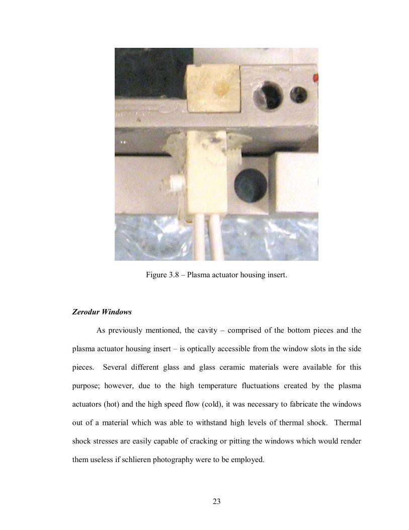
Figure 3.8 – Plasma actuator housing insert.

Zerodur Windows

As previously mentioned, the cavity – comprised of the bottom pieces and the

plasma actuator housing insert – is optically accessible from the window slots in the side

pieces. Several different glass and glass ceramic materials were available for this

purpose; however, due to the high temperature fluctuations created by the plasma

actuators (hot) and the high speed flow (cold), it was necessary to fabricate the windows

out of a material which was able to withstand high levels of thermal shock. Thermal

shock stresses are easily capable of cracking or pitting the windows which would render

them useless if schlieren photography were to be employed.

24

Zerodur, manufactured by SCHOTT, is a glass ceramic with an extremely low

coefficient of thermal expansion. This allows it to withstand a large amount of thermal

and thermal shock stresses without causing structural damage to the material. Zerodur is

also easily machinable and is non-porous which allows it to maintain its properties for a

long period of time (SCHOTT Zerodur 2005). These properties are what make Zerodur

one of the main materials used for land based and orbiting telescope lenses.

For the window, the thermal stresses in this experiment will be negligible. The

mean temperature for the flow will determine the thermal stress. As the flow velocity

increases, the temperature drops. Since the coefficient of thermal expansion is positive,

the window will shrink by a very small amount. The nozzle is exhausting to ambient air

so the pressure difference between the inside and outside of the window is relatively

small. Therefore, the thermal and mechanical stresses are negligible. The thermal shock

stresses are the most pertinent stress that the window will be exposed to for this

application. The thermal shock stress can be calculated for the window, regardless to

geometry, by

TEfw ∆−

=µ

ασ1

(5)

where σw is the thermal shock induced stress, f is the thermal usage factor, α is the

coefficient of thermal expansion, E is Young’s modulus, µ is Poisson’s ratio, and ∆T is

the change in temperature (SCHOTT TIE: 32 2004). For Zerodur, α = 0.05 x 10-6 K-1, E

= 90 GPa, µ = 0.24, and for this research the usage factor f was assumed to be the worst

case or 1.00 and the temperature difference was estimated to be 600 K. The maximum

thermal shock stress that Zerodur can handle is 20 MPa before fracture or other stress

related damage occurs (Davis 2005). Based on Equation 5, the thermal shock stress for

25

this particular scenario was 3.60 MPa which gives a factor of safety of 5.55 which was

sufficient. The windows designed for the cavity flow assembly can be seen in Figure 3.9.

Figure 3.9 – Zerodur window for optical accessibility.

Data Acquisition

In all of the experiments conducted for this research, data is acquired using two

different methods. The first method involves static pressure measurements. This is done

by placing a probe or tap on the edge of a flow. Since a flow has zero velocity at the

boundary condition or wall, a measurement of the static pressure requires a probe located

at the wall connected to a pressure gauge. On the top piece of the extension there are

twelve static pressure taps. The taps are connected to a pressure multiplexer using 1/16”

inner diameter plastic tubing. The pressure multiplexer allows each static pressure tap to

be checked by turning the dial on the multiplexer and reading the pressure on the gauge.

26

The experimental setup showing the pressure measurement equipment can be seen in

Figure 3.10.

Figure 3.10 – Experimental setup showing pressure testing equipment.

The second method involves a Kulite pressure transducer, XCEL-072-25A. The

XCEL-072 has a natural frequency of 400 kHz. The sensitivity for this particular

transducer was 4.062 mV/psi. The Kulite transducer was placed through the bottom front

piece to record the pressure fluctuations within the cavity. The transducer was excited,

amplified, and low pass filtered at 50 kHz using a Barton signal conditioner. The signal

27

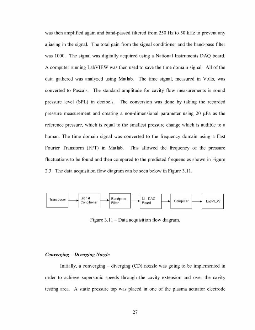
was then amplified again and band-passed filtered from 250 Hz to 50 kHz to prevent any

aliasing in the signal. The total gain from the signal conditioner and the band-pass filter

was 1000. The signal was digitally acquired using a National Instruments DAQ board.

A computer running LabVIEW was then used to save the time domain signal. All of the

data gathered was analyzed using Matlab. The time signal, measured in Volts, was

converted to Pascals. The standard amplitude for cavity flow measurements is sound

pressure level (SPL) in decibels. The conversion was done by taking the recorded

pressure measurement and creating a non-dimensional parameter using 20 µPa as the

reference pressure, which is equal to the smallest pressure change which is audible to a

human. The time domain signal was converted to the frequency domain using a Fast

Fourier Transform (FFT) in Matlab. This allowed the frequency of the pressure

fluctuations to be found and then compared to the predicted frequencies shown in Figure

2.3. The data acquisition flow diagram can be seen below in Figure 3.11.

Figure 3.11 – Data acquisition flow diagram.

Converging – Diverging Nozzle

Initially, a converging – diverging (CD) nozzle was going to be implemented in

order to achieve supersonic speeds through the cavity extension and over the cavity

testing area. A static pressure tap was placed in one of the plasma actuator electrode

28

holes to obtain the pressure at the leading edge of the cavity. The stagnation pressure

was raised in small increments and then the Mach number was calculated using the

standard isentropic formula relating Mach number to pressure ratio is shown below in

Equation 6,

12

211

−

−+=

γγ

γ MPPo (6)

where Po/P is the ratio of absolute stagnation pressure to absolute static pressure, γ is the

ratio of specific heats, and M is the Mach number (Anderson 2004). The pressures were

recorded and several attempts were made to achieve supersonic flow velocity over the

cavity. However, after multiple trials, supersonic velocity could not be achieved. As the

stagnation pressure was increased, the static pressure at the leading edge of the cavity

continued to rise linearly as well. For a properly designed nozzle, this is to be expected

once its design pressure ratio is reached; however, for the Mach 1.3 nozzle, this velocity

had not yet been achieved. The static pressure and Mach number at the cavity edge can

be seen in Figure 3.12 below. As Equation 6 shows, the ratio of the absolute stagnation

pressure to the absolute static pressure must reach a certain value before the flow will

become supersonic. Since the static pressure continued to rise linearly with an increase

in stagnation pressure before reaching the ideal operating conditions of the converging –

diverging Mach 1.3 nozzle, it was not possible to achieve a higher velocity. As the Mach

number versus stagnation pressure graph shows – Figure 3.12 – the limit of the velocity

was approximately Mach 0.78.

29

Figure 3.12 – Converging – diverging nozzle Mach number over cavity.

Since it was unknown why the flow was unable to achieve faster velocities,

several modifications were made to the facility. Static pressure taps were placed in the

top piece of the extension starting 0.25” before the cavity to 1.50” passed it. They were

evenly spaced at 0.25” to increase the resolution of the pressure as it progressed over the

cavity. Also, the CD nozzle was exchanged for a converging nozzle. The dimensions are

the same for both the converging and converging – diverging nozzles, so the switch

between the two nozzles was an easy modification in the experiment. The experiment

was repeated to try to achieve as high a velocity as possible over the cavity with the

knowledge that only subsonic speeds are attainable with the implementation of the

30

converging nozzle. Figure 3.13 shows the Mach number of the flow as it progresses over

the cavity.

Figure 3.13 – Converging nozzle Mach number over cavity.

As Figure 3.13 shows, as the Mach number was increased at the leading edge, the

velocity continued to increase as the flow progressed over and passed the cavity. The

flow separates from the leading edge of the cavity, since it cannot follow the contour (90°

bend) of the cavity, creating a shear layer. As the shear layer travels over the cavity it

continues to grow. The growth of the shear layer causes the rest of the freestream flow to

be channeled between the shear layer and the top of the extension. This reduced area

31

causes the velocity to increase since velocity and area are directly proportional and mass

must be conserved. At these velocities, the air must be modeled using compressible flow

analysis. Taking this into consideration and by comparing the results shown in Figure

3.13, the flow was choking, or reaching Mach 1.0, downstream of the cavity. Mach 1.0

was the highest velocity that can be achieved without diverging the flow. Since the flow

is choking downstream of the cavity, subsonic velocities can only be explored unless

modifications are made to the cavity extension. As Figure 3.13 shows, the increase in

velocity over the cavity was negligible up to Mach 0.60, approximately 3%, which was

consistent with past experiments (Debiasi and Samimy 2004). Therefore, Mach 0.60 was

the flow velocity limit over the cavity with the current extension configuration.

Plasma Generation Method

The localized arc filament plasma actuators (LAFPA) used in this research were

powered using an in house system developed at the GDTL. The electric discharge which

creates the plasma was controlled using LabVIEW. The frequency, duty cycle, and the

phase of each actuator can be controlled from the computer. A National Instruments

digital-to-analog converter was then connected to an EMI filter. The EMI filter is a

safety on/off switch for the plasma. When the EMI affects the computer, it is not

possible to shut the plasma off using LabVIEW. The EMI filter has an optical switch

which is immune to electro-magnetic interference. This allows the plasma to be turned

off from a simple toggle switch even if the computer has crashed. The EMI filter is

connected to the plasma generation system which consists of an AC and DC power

systems, ballast resistors, and fast response transistor switches (Samimy et al. 2004a).

32

With the current configuration, the plasma actuator power coupled to the flow is in the

range of 40 – 100 W. The plasma generation block diagram can be seen in Figure 3.14

shown below.

Figure 3.14 – Plasma generation block diagram.

One of the major unknowns in this research experiment was the generation of

plasma in a confined cavity flow. LAFPA’s had already been used and verified in jet

applications; but, there had been no attempt to generate an arc of plasma close to

aluminum side walls and other sensitive electronic equipment, such as the Kulite pressure

transducer (Samimy et al. 2004b). One of the initial tests on the cavity extension was to

determine if plasma could be used in this case. As Figure 3.15 shows, based on the blue

glow and arc visible through the window of the facility, plasma actuators could create

plasma in the flow; and, the Kulite pressure transducers could still be used to detect the

pressure fluctuations even with a significant source of EMI only a few millimeters away.

33

Figure 3.15 – Plasma actuator arc in cavity.

34

CHAPTER 4

EXPERIMENTAL RESULTS

Facility Characterization

The first step in obtaining experimental results from the cavity extension was to

characterize the flow through the extension. The cavity extension was installed on the

converging nozzle since only subsonic velocities were studied at this time. In order to

characterize the flow through the extension, a Mach sweep was performed. This was

done to determine the broadband noise level and to also determine which cavity tones, if

any, were being generated. This sweep would also determine if the pressure fluctuations

were cavity tones: single mode or multi-modal.

The stagnation pressure was started at 0.50 psig and then increased in small

increments up to 6.00 psig. This corresponds to a sweep from Mach 0.26 to Mach 0.68.

At each stagnation pressure, the data collected from the Kulite pressure transducer was

recorded using LabVIEW. The sound pressure level (SPL) was calculated for each data

set, and the stagnation and the static pressure ratio was converted to Mach number.

Matlab was then used to create a spectrogram showing the correlation between Mach

number, frequency, and amplitude. An interpolation algorithm was performed to smooth

out the transition points between all of the data sets. Figure 4.1 shows the sound pressure

35

level and Mach number. The amplitudes of the SPL are color coded. The red color

indicates stronger amplitudes while the blue shows weaker amplitudes.

Figure 4.1 – Spectrogram for facility characterization.

As Figure 4.1 shows, the broadband noise energy increases with the increase in

Mach number. In order to determine which tones were being generated, the predicted

acoustic and Rossiter modes were imposed onto the spectrogram. This is shown in

Figure 4.2. For flows less than Mach 0.45, the pressure fluctuations followed the 2nd

Rossiter mode. When the flow velocity was greater than 0.45, the tones switched to the

3rd Rossiter mode. As Figure 4.2 shows, when the 3rd Rossiter, the 1st Transverse, and the

SPL(dB)

36

2nd Lateral intersected from Mach 0.48 to 0.55, the SPL was almost 140 dB. This shows

that the cavity acoustic was coupling with the Rossiter mode and generating single mode

cavity tones.

Figure 4.2 – Spectrogram for facility characterization with cavity tones.

The sound pressure levels from the Mach sweep were used to identify the baseline

cases which would serve as the test cases for the plasma actuators. Based on this Mach

number sweep, the baseline cases were chosen as Mach 0.55 and Mach 0.60. Mach 0.55

exhibits a strong cavity tone while Mach 0.60 does not. These two flows will be used to

determine the effectiveness of the plasma actuators in this facility.

SPL(dB)

37

Mach 0.55 Plasma Actuation

The Mach 0.55 flow was chosen as a flow field where plasma actuation would be

tested because the SPL revealed a strong cavity tone at approximately 9 kHz. Also, the

source of this cavity tone was identified as the 3rd Rossiter mode from the facility

characterization experiments which can be seen in Figure 4.2. The first step was to

acquire the sound pressure level for the baseline case. After the baseline SPL was

obtained, the plasma actuators were used to try to control the flow field.

Although the plasma actuator housing insert was designed to hold three

independent plasma actuators, one of the plasma actuators was inoperable. During

facility characterization part of the boron nitride ceramic cracked and broke away from

the outer edge. This section was reattached using 2-ton epoxy. However, after the

testing was conducted, a larger section had cracked and broken in the piece. This made it

impossible to insert a steel electrode into this slot. This left two actuators operable for

the experiment.

For this set of experiments, only one plasma actuator was used. The center

actuator was used in order to keep the flow symmetric and as two dimensional as

possible. LabVIEW was used to control the plasma actuators. The duty cycles and

actuation frequencies used during all of the experiments conducted using plasma

actuation can be seen in Table 4.1. Although multiple actuation frequencies were

explored, only a subset is shown which was indicative of the rest of the data. Figure 4.3

shows the baseline SPL and the SPL when the plasma actuator was in use. In Figure 4.3,

the frequency that the plasma actuator was operated at is indicated in the title above each

38

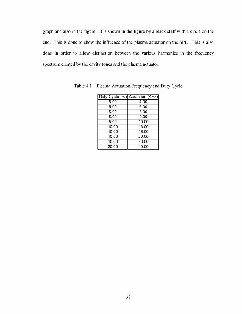
graph and also in the figure. It is shown in the figure by a black staff with a circle on the

end. This is done to show the influence of the plasma actuator on the SPL. This is also

done in order to allow distinction between the various harmonics in the frequency

spectrum created by the cavity tones and the plasma actuator.

Table 4.1 – Plasma Actuation Frequency and Duty Cycle

Duty Cycle (%) Acutation (KHz)5.00 4.005.00 6.005.00 8.005.00 9.005.00 10.0010.00 13.0010.00 16.0010.00 20.0010.00 30.0020.00 40.00

39

Figure 4.3 – SPL with center plasma actuation at Mach 0.55.

The figures in Figure 4.3 show that the plasma actuator is capable of generating

sound pressure levels of 126 and 128 dB at an actuation frequency of 6 and 13 kHz,

respectively. When the LAFPA was actuated at 9 kHz, which was close to the cavity

tone, the actuation SPL cannot be distinguished from the 3rd Rossiter mode except for the

higher order harmonics seen at 27 and 36 kHz. It is important to note that even though

the plasma actuator was generating a tone at almost the exact same frequency of the

cavity tone, it did not affect the dominate cavity tone at all. For each case at Mach 0.55,

40

the one center plasma actuator did not cause any notable modifications to the broadband

SPL or the cavity tone.


The second case tested using plasma actuation was Mach 0.60. In this flow field,

there was not a strong cavity tone as in the Mach 0.55 experiment. The frequencies used

for plasma actuation were the same as the Mach 0.55 case. These can be seen in Table

4.1. In each frequency used at Mach 0.60, the plasma actuator was capable of generating

a tone at that frequency of about 125 dB for 6 and 9 kHz. This can be seen in Figure 4.4

below. However, at the higher frequency actuation, 20 + kHz, the pressure perturbation

was significantly larger. In fact, the pressure perturbation created by the plasma actuator

was more significant than the original flow field created. This phenomenon was detected

in the Mach 0.55 flow as well, which can be observed in Figure 4.3.

41


As mentioned earlier, the shear layer was being influenced in the receptivity

region of the flow or at the leading edge of the cavity where it forms. The flow field can

be modeled using Navier-Stokes equations. However, the Navier-Stokes model is a set

of nonlinear partial differential equations which solves for a complete solution of the

flow field (Pope 2000). Except for a few very specific cases, the equations are not

solvable. The important aspect of the Navier-Stokes equations is their nonlinearity. This

means that even a small change in the boundary layer and in the initial conditions can

propagate through the system to create any number of changes in the flow field. This is

42

what was occurring at these higher frequency perturbations. The high frequency forcing

changed the flow and created these very pronounced and strong cavity tones within the

flow.

Unfortunately, even at these higher frequency pressure perturbations, the one

center plasma actuator was incapable of changing the flow. There was not any

observable change in the background noise level or the sound pressure level of the small

tones generated by the flow.


Mach 0.48 was chosen as a baseline case after the first two cases, Mach 0.55 and

0.60, were already explored. This was done to determine if the energy of the flow was

dominating the energy produced by the plasma actuator. Since the energy of the flow is

directly proportional to the square of the velocity, this reduction from Mach 0.55 and

0.60 to Mach 0.48 was quite significant.

Figure 4.5 shows the baseline SPL for the Mach 0.48 flow field. This is another

instance of a strong cavity tone flow situation. The other figures shown in Figure 4.5 are

similar to the previous experiments for Mach 0.55 and 0.60. The plasma actuator was

excited with several different frequencies to create the pressure perturbations in the shear

layer. As in the previous cases, the plasma actuator did not have any noticeable effect on

the pressure fluctuations within the cavity. This included the cavity tone and the

background noise level.

43


Asymmetric Plasma Actuation

The main shortcoming of using only the center plasma actuator was that it could

not influence the entire development of the shear layer as it separated from the leading

edge of the cavity. The distance between two electrodes, which constitutes one plasma

actuator, is 3.0 mm. This is a very small percentage of the length of the shear layer,

which is 1.50” long. As mentioned earlier in this chapter, only two plasma actuators

could be used since part of the plasma actuator housing insert broke. The major

downside to this development is that using two plasma actuators would create an

44

asymmetric flow field over the cavity. This could potentially create an unpredictable

flow field.

Figure 4.6 shows the baseline SPL and the SPL for five different actuation

frequencies. Even with two actuators, the sound pressure level produced by the plasma

actuator was approximately 126 dB. When compared to the sound pressure levels

obtained using only the center actuator, Figure 4.4, the two plasma actuators caused the

same results. In each case, the plasma actuator did not cause any detectable change in the

pressure fluctuations present within the cavity. Although only the Mach 0.60 case is

shown, the results obtained for the other Mach numbers were similar for the asymmetric

actuation. Like before with one actuator, this suggests that the energy of the flow was not

the factor which caused ineffectual actuation of the shear layer.

45

Figure 4.6 – SPL with asymmetric plasma actuation at Mach 0.60.

46

CHAPTER 5

CONCLUSION AND FUTURE WORK

Previous research at the Gas Dynamics and Turbulence Laboratory showed that a

compression actuator was capable of attenuating pressure fluctuations in the cavity by up

to 20 dB in a Mach 0.30 flow. However, at higher Mach numbers, the compression

actuator was incapable of generating actuation with sufficient bandwidth or amplitude in

order to influence the developing shear layer and hence the cavity tones generated by the

flow. Localized arc filament plasma actuators were developed which are capable of

generating pressure perturbations with a very broad frequency range and with strong

amplitudes. This research focused on using LAFPA’s to create the necessary pressure

perturbations to reduce the strong pressure fluctuations present within a cavity flow. The

experiments were conducted in a free jet facility at Mach 0.48 to Mach 0.60.

A cavity extension was developed which enclosed an existing converging

rectangular nozzle. The extension had an adjustable cavity length from 1.00” to 1.50”.

For all of the experiments conducted in this research, the length of the cavity was set to

1.00”. The depth of the cavity was 0.27” which resulted in an aspect ratio of 3.70, or a

shallow cavity. Twelve static pressure taps were inserted through the extension to

measure the Mach number of the flow field as it passed over the cavity and out of the

extension. This was used to evaluate the velocity asymptote at Mach 0.78 which the

47

extension could not surpass. It was determined that the flow was choking downstream of

the cavity, and thus limiting the flow in the cavity to subsonic velocities.

The plasma actuator housing was constructed of a machinable boron nitride

ceramic. The steel electrodes were placed 2.00 mm away from the leading edge of the

cavity. The center to center distance between a pair of electrodes was 3.00 mm which

were also countersunk by 0.50 mm to prevent the plasma from becoming unstable.

The cavity extension was characterized by performing a Mach number sweep

from 0.28 to 0.68. The cavity pressure levels were recorded using Kulite pressure

transducers, data acquisition equipment, and LabVIEW. The measurements were

converted to non-dimensional sound pressure level for comparison. All data processing

and figure creation was done using Matlab.

Plasma actuators were used to create pressure perturbations at the receptivity

region of the shear layer located at the leading edge of the cavity. Test cases of Mach

0.48, 0.55, and 0.60 were chosen based on the presence of strong and weak cavity tones

and also the energy of the flows. Initially, one plasma actuator was used to determine if

there was any noticeable effect on the flow. In each test case, there was neither a

reduction in the amplitude of the cavity tones nor a reduction in the overall background

noise level. This occurred in both the high energy flows as well as the lower energy

flows.

One of the major accomplishments of this research project was the use of plasma

actuators in a cavity flow. This experiment shows that it is indeed possible to generate

plasma in a confined cavity flow. The actuators did not arc in unwanted locations or

ground to the aluminum sidewalls. Also, the pressure fluctuations were able to be

48

acquired even with the Kulite pressure transducers located only millimeters away from

the plasma actuators. The EMI produced by the LAFPA’s was not a hindrance to the

successful acquisition of data.

In order to resolve some of the issues encountered in this research project, several

changes can be implemented which would resolve some of these problems. One of the

troublesome aspects of this entire project was the plasma actuator housing. The initial

design for the boron nitride piece, shown in Figures 3.7 and 3.8, was not robust. When

the steel electrodes were inserted, plastic set screws were used to keep them in place.

However, after the first use, the threads stripped out of the boron nitride. From this point

on, the electrodes were glued into place. Since they could no longer be removed, the tips

could not be cleaned and different electrodes, such as tungsten, could not be tested. Also,

as mentioned earlier, one of the corner pieces broke twice. The first time it was repaired,

but the second time left the third actuator inoperable. All of these failures were caused

by design and not operating conditions from the experiment. This means that a redesign

is needed to fix these issues.

The second problem encountered was the limitation of the flow to subsonic

velocities. Even with the use of a converging – diverging nozzle, the flow velocity could

not be increased passed Mach 0.78. One method to hurdle this obstacle would be to

diverge the cavity extension downstream of the flow. As the shear layer grows, the

height of the extension would increase as well. This would help prevent a choke point

from developing in the extension and thus allow supersonic velocities to be obtained.

Another method to circumvent this issue is the reduction in depth of the cavity. This

49

would retard the growth of the shear layer and also help reduce the chance of the nozzle

extension choking downstream of the flow.

Some of the recommendations for future work will be made as this research

progresses. The study of high speed cavity flows is quite complex and will require more

work in order to successfully suppress the strong cavity tones produced from the flow

over the cavity. The experiments begun in this research will be continued at the Gas

Dynamics and Turbulence Laboratory in fulfillment of a Masters in Mechanical

Engineering at The Ohio State University.

50

REFERENCES

Anderson, John D., Modern Compressible Flow: With Historical Perspective. 3rd ed. Boston: McGraw-Hill Education, 2004.

Cattafesta, L., Garg, S., Choudhari, F., Li, F. “Active Control of Flow-Induced Cavity

Resonance.” AIAA Paper 97-1804, 1997. Cattafesta, L., Williams, D., Rowley, C., Alvi, F. “Review of Active Control of Flow-

Induced Cavity Resonance.” AIAA Paper 2003-3567, 2003. Davis, Dr. Mark. Technical Phone Consultation, SCHOTT North America, Inc. 4

October 2005. Debiasi, M. and Samimy, M. “Logic-Based Active Control of Subsonic Cavity Flow

Resonance.” AIAA Journal 42.9 (2004): 1901-1909. Halliday, D., Resnick, R., Walker, J. Fundamentals of Physics: Extended. 6th Ed. New

York: John Wiley & Sons, Inc., 2001. Little, J. “Development and Application of a Visualization Technique for Baseline and

Controlled Cavity Flow.” Undergraduate Thesis, 2004. McGregor, O. W. and White, R. A. “Drag of Rectangular Cavities in Supersonic and

Transonic Flow Including the Effects of Cavity Resonance.” AIAA Journal 8.11 (1970): 1959-1964.

Pope, Stephen B. Turbulent Flows. New York: Cambridge University Press, 2000. Rossiter, J.E. “Wind Tunnel Experiments on the Flow over Rectangular Cavities at

Subsonic and Transonic Speeds.” RAE TR 64037 and Aeronautical Research Council, Repts. and Memoranda No. 3438 (1964).

Rowley, C., Juttijudata, V., Williams, D. “Cavity Flow Control Simulations and

Experiments.” AIAA Paper 2005-0292, 2005. Samimy, M., Adamovich, I., Kim, J.-H., Webb, B., Keshav, S., Utkin, Y. “Active Control

of High Speed Jets Using Localized Arc Filament Plasma Actuators.” AIAA Paper 2004-2130, 2004a.

51

Samimy, M., Adamovich, I., Webb, B., Kastner, J., Hileman, J., Keshav, S., Palm, P. “Development and characterization of plasma actuators for high-speed jet control.” Experiments in Fluids 37 (2004b): 577-588.

Samimy, M., Debiasi, M., Caraballo, E., Malone, J., Little, J., Özbay, H., Efe, P., Yan, P.,

Yuan, X., DeBonis, J. “Exploring Strategies For Closed-Loop Cavity Flow Control.” AIAA Journal 2004-0576 (2004c): 1-16.

Samimy, M., Kim, J.-H., Adamovich, I., Utkin, Y., Kastner, J. “Active Control of High

Speed and High Reynolds Number Free Jet Using Plasma Actuators.” AIAA Paper 2006-0711, 2006.

SCHOTT North America, Inc. “TIE-32: Thermal loads on optical glass.” August 2004.

<http://www.us.schott.com/optics_devices/english/download/tie-32_thermal_loads_on_optical_glass_us.pdf>.

SCHOTT North America, Inc. “Zerodur: Product Information.” October 2005.

<http://www.us.schott.com/optics_devices/english/products/zerodur/index.html>. Stanek, M., Raman, G., Kibens, V., Ross, J., Odedra, J., Peto, J. “Suppression of Cavity

Resonance Using High Frequency Forcing – The Characteristic Signature of Effective Devices.” AIAA Paper 2001-2128, 2001.

Williams, D., Rowley, C., Colonius, T., Fabris, D., Albertson, J. “Model-Based Control

of Cavity Oscillations – Part 1: Experiments.” AIAA Paper 2002-0971, 2002.

52

APPENDIX A

Three Dimensional Wave Numbers and Frequencies

m n q k f (Hz)0 0 0 0 00 0 1 82 41490 0 2 165 82980 1 0 161 80830 1 1 181 90850 1 2 230 115840 2 0 321 161650 2 1 332 166890 2 2 361 181711 0 0 124 62241 0 1 149 74801 0 2 206 103731 1 0 203 102011 1 1 219 110131 1 2 261 131501 2 0 344 173221 2 1 354 178121 2 2 382 192072 0 0 247 124472 0 1 261 131202 0 2 297 149602 1 0 295 148412 1 1 306 154102 1 2 338 170032 2 0 405 204022 2 1 414 208202 2 2 438 22025

53

APPENDIX B

Engineering Drawings for Cavity Extension

54

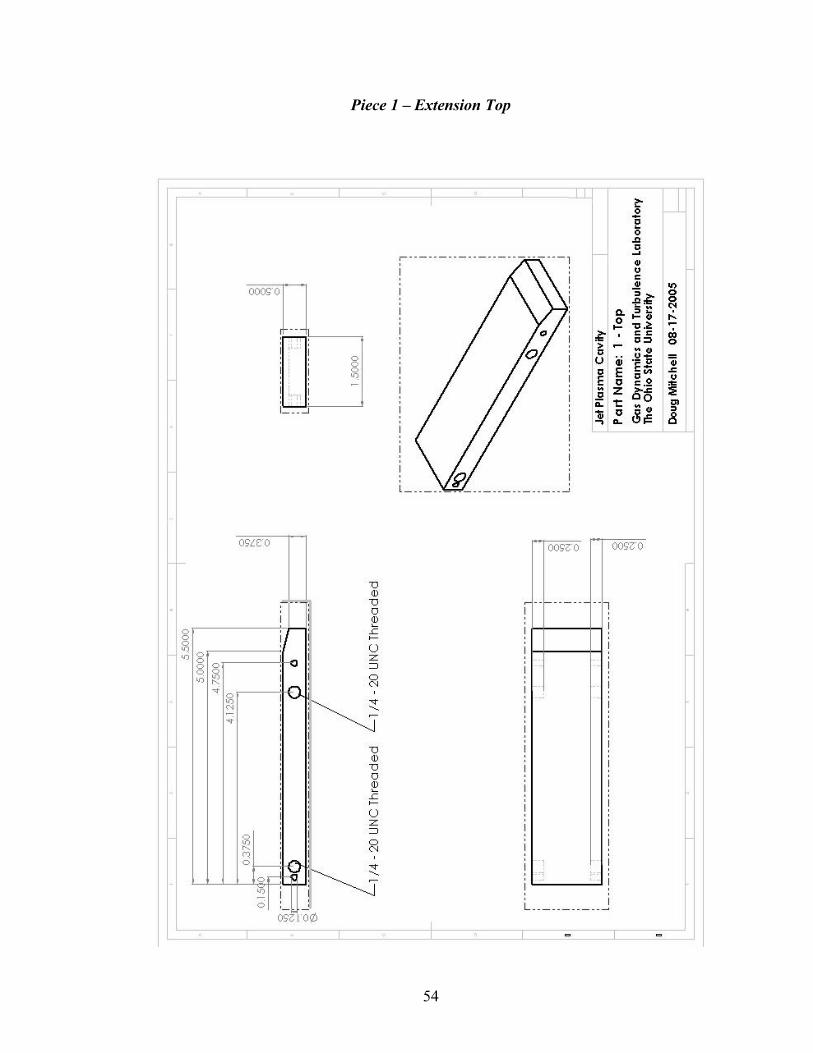
Piece 1 – Extension Top

55

Piece 2 – Bottom Front

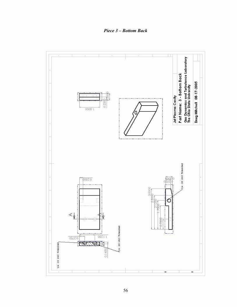
56

Piece 3 – Bottom Back

57

Piece 4 – Ceramic Insert

58

Piece 5 – Window

59

Piece 6 – Side Left

60

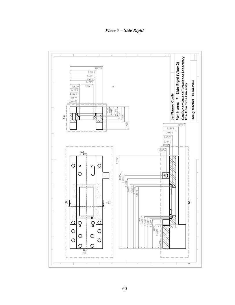
Piece 7 – Side Right

61

Piece 8 – Window Plate

62

Piece 9 – Side Brackets

CONTROL OF HIGH SPEED CAVITY FLOW USING PLASMA …

Documents

Transcript of CONTROL OF HIGH SPEED CAVITY FLOW USING PLASMA …