Department of Computer Science and Engineering CHALMERS UNIVERSITY OF TECHNOLOGY UNIVERSITY OF GOTHENBURG Göteborg, Sweden, May 2009

Control of a wind turbine equipped with a variable rotor resistance HÉCTOR A. LÓPEZ CARBALLIDO

THESIS FOR THE DEGREE OF MASTER OF SCIENCE

Control of a wind turbine equipped with a variable rotor resistance

HÉCTOR A. LÓPEZ CARBALLIDO

Department of Energy and Environment

Division of Electric Power Engineering

CHALMERS UNIVERSITY OF TECHNOLOGY

Göteborg, Sweden, May 2009

Control of a wind turbine equipped with a variable rotor resistance

© HÉCTOR A. LÓPEZ CARBALLIDO, 2009.

Department of Energy and Environment

Division of Electric Power Engineering

CHALMERS UNIVERSITY OF TECHNOLOGY

Göteborg, Sweden, May 2009

iii

Abstract

In this thesis the control of a wind turbine equipped with an induction generator with a variable rotor resistance was investigated. Analysis, modelling and control of the induction generator system was conducted. In particular the focus was put on the reduction of torque fluctuations, in order to reduce the stresses in the gearbox and in the mechanical structure as well as reducing the flicker emission.

Different controlling methods were studied in order to find an appropriate choice. Finally, the induction machine with the variable rotor resistance controller was compared with the same induction machine without controller for the wind application, in order to study the improvement of implementing the controller.

The first thing to be emphasized is that by utilising the controller the flicker contribution can be reduced between 35%‐60% compared to the uncontrolled system. It was also found that the reduction of the flicker contributions was strongly related with the turbulence intensity in the wind. The reduction in the flicker emission was stronger for more turbulent winds. Furthermore, a reduction in the magnitude of the electrical torque components for the frequencies above 1Hz was found. Those high‐frequency components are the ones that more contribute to the mechanical stresses in the gearbox and structure of the turbine, this means that by utilising the controller there will be less tear and wear on the mechanical parts of the turbine.

iv

v

Acknowledgement

First of all, I would like to thank my supervisor at Chalmers University of Technolgy, Assoc. Prof. Torbjörn Thiringer for his encouraging and inspiring attitude. I also would like to thank to Prof. Stefan Lundberg, for theoretical help and discussions.

Finally, I would like to thank the whole department, especially to the master thesis students that were preparing their thesis at the same time as me, for a nice working atmosphere and kind treatment during my stay in Sweden.

Héctor López

May, 2009

vi

vii

Contents Abstract .......................................................................................................................................iii

Acknowledgement ........................................................................................................................v

Chapter 1 Introduction............................................................................................................... 1

1.1 Background .................................................................................................................... 1

1.2 Previous work ................................................................................................................ 2

1.3 Goal of the project ........................................................................................................ 2

1.4 Thesis layout .................................................................................................................. 2

Chapter 2 Wind turbines & offshore wind parks ....................................................................... 3

2.1 Wind turbines ................................................................................................................ 3

2.1.1 Aerodynamic conversion ....................................................................................... 3

2.1.2 Fixed and variable speed wind turbines ................................................................ 4

2.2 Offshore wind farms ...................................................................................................... 6

2.3 HVDC lines ..................................................................................................................... 7

2.4 Power quality characteristics of wind turbines ............................................................. 7

Chapter 3 Induction machine ..................................................................................................... 9

3.1 Induction machine as wind turbine generator .............................................................. 9

3.2 Induction machine modelling ...................................................................................... 10

3.3 Linearization of the induction machine model ........................................................... 14

3.4 Induction machine with extra rotor resistance ........................................................... 17

3.5 Parameters of a generic 2MW induction machine ..................................................... 20

Chapter 4 Design of the controller for the extra rotor resistance ........................................... 21

4.1 Model of the linearized 2MW induction machine ...................................................... 21

4.1.1 Order reduction of the linearized model ............................................................ 25

4.2 Design of the controller ............................................................................................... 31

4.2.1 High‐pass filter .................................................................................................... 32

4.2.2 Proportional controller ........................................................................................ 34

4.2.3 Proportional‐Integral controller .......................................................................... 38

4.2.4 Double integrator controller ............................................................................... 39

Chapter 5 Evaluation of the controller .................................................................................... 43

5.1 Response of the system to synthetic curves ............................................................... 43

5.2 Response of the system to real shaft torque data ...................................................... 46

viii

5.2.1 Flicker reduction .................................................................................................. 49

5.2.2 Mechanical stresses reduction ............................................................................ 51

5.2.3 Energy losses in the induction machine .............................................................. 52

Chapter 6 Final specifications of the controller based on the evaluations ............................. 55

6.1 Selection of the cut‐off frequency and the proportional gain .................................... 55

6.2 Selection of the default external rotor resistance ...................................................... 58

6.3 Final specifications ...................................................................................................... 59

Chapter 7 Conclusions.............................................................................................................. 61

Chapter 8 Proposed future work ............................................................................................. 63

References ..................................................................................................................................61

1

Chapter 1

Introduction

1.1 Background

Wind power is without any doubt becoming an important energy source. Today a massive expansion is going on. However, the possible sites on land are starting to get fewer and accordingly the focus on sea locations are growing. Here there is much more space, and not only that, a higher average wind speed is available, because wind speeds are affected by the friction against the earth´s surface, and since the surfaces of the sea is very smooth and the obstacles to the wind are few, the average wind speed is higher than on land.

For these reasons, offshore wind energy is a promising solution for countries with high population density and without suitable sites on land to build wind parks. Of course, there are some limitations for the construction of offshore wind farms like that costs are higher than on land, but the energy production is also higher.

However, cables are needed and then only 100 km of energy transportation is possible if 50 Hz AC is used. Since large‐scale electric power has to be transmitted over long distances, then HVDC lines are needed, and the first such park is today being built in the North Sea. Furthermore, HVDC transmission systems have been in successful operation in power systems all over the world for about 40 years, and there are some well‐known and accepted facts that can be very useful for offshore wind parks. The most important is that the offshore grid and onshore grid are isolated by the HVDC‐link, this gives new possibilities regarding the local AC‐system which can be utilised.

In this local AC‐system the voltage and frequency can be changed by the AC‐DC converter in the offshore side. This open the possibility of removing the converter connected to the generator of each wind turbine, but still having variable rotor speed in the turbines thanks to a central speed control for the whole wind farm that can changes the frequency of the grid, hence the speed of the wind turbines, which are equipped with induction generators directly connected to the electrical grid. This will reduce the cost for the wind turbine system, and in addition increase the reliability. Here the system with a variable rotor resistance becomes of high interest, since it can reduce mechanical stresses on the turbine just as a variable speed system.

A very interesting issue for this system with variable rotor resistances is to what extent this system can be used for this application, and the selection of a suitable control. With a controllable rotor resistance it will be possible to absorb incoming power variations by changing the rotor speed much faster than the pitch controller, which will give a better power quality.

2

1.2 Previous work

The control of an external rotor resistance has been studied before, for example the ©OptiSlip concept by the Danish manufacturer Vestas. But there is not too much available literature about this subject in particular for the situation where voltage an frequency can change. In [1] a derived control law for a wind turbine using variable rotor resistances is found, but in that paper only the flicker contribution of the wind turbine is studied.

1.3 Goal of the project

The main purpose of this thesis is to investigate how a wind turbine using a variable rotor resistance can be controlled for a wind turbine application. For this purpose an induction machine will be modelled and linearized. Moreover, an objective is to study how this system behaves for a situation with realistic wind inputs.

1.4 Thesis layout

The body of the thesis is organized as follows:

Chapter2, description of common wind turbines systems and offshore wind farms.

Chapter 3, presentation of the induction machine model and it linearization.

Chapter 4, presents the design of the controller.

Chapter 5, presentation of the results for different shaft torque curves, synthetic and real data.

Chapter 6, describes the final design of the controller and its final characteristics.

Chapter 7, gives a summary of the conclusion that could be extracted from the results of the evaluations.

Chapter 8, contains the proposed future work.

3

Chapter 2

Wind turbines & offshore wind parks

This chapter gives a brief overview of common wind turbine systems. It also introduces the advantages of combine offshore wind parks with HVDC lines. The interested reader can find more information about wind turbine theory in [16], about offshore wind farms in [17] and about HVDC lines in [15].

2.1 Wind turbines

2.1.1 Aerodynamic conversion

A wind turbine system gets its input power by converting some of the kinetic energy in the wind into torque acting on the rotor blades. This process is called the aerodynamic conversion, and depends on the wind speed, the rotor area, the pitch angle of the blades, and the density of the air. Although there are different types of wind turbines systems, all of them work in a similar way.

In order to calculate the mechanical power from a wind turbine the Cp(β,λ) curve can be used. With this knowledge the mechanical power can be determined by

, (2.1)

Where Cp(β,λ) describes how much of the available energy in the wind that can be converted into mechanical power that depends on the tip speed ratio λ and in the pitch angle of the blades β, ρ is the air density, Ar is the area swept by the rotor and w is the wind speed. A typical Cp(β,λ) is presented in the figure 2.1, where it is possible to see the Cp(λ) curves for different values in the pitch angle of the blades.

4

Figure 2.1, typical Cp(β,λ) curve.

The wind turbine starts to generate energy when the wind speed is above Vcut‐in and stops when the wind speed is above Vcut‐off. Figure 2.2, shows an example of how the mechanical power varies with the wind speed.

Figure 2.2, typical power curve of a wind turbine

2.1.2 Fixed and variable speed wind turbines

Fixed‐speed system

The fixed speed wind turbines [11] have been the standard wind turbines for several decades due to its simplicity and robustness. For the fixed speed operation the stator of the induction generator is directly connected to the grid. Then the rotor shaft is almost locked to

0 2 4 6 8 10 12 14 16 18 200

0.1

0.2

0.3

0.4

0.5

Lambda

Cp

B=-3B=-1B=1B=3B=5B=10B=15

0 2 4 6 8 10 12 14 16 18 200

500

1000

1500

2000

Wind Speed (m/s)

Pow

er (k

W)

5

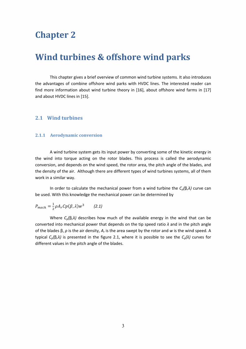
the frequency of the grid, admitting only very small speed variation from the nominal value. Figure 2.3 shows the principal layout of such a system.

Gearbox IM Grid

Soft starter

Bankcapacitor

Figure 2.3, fixed‐speed wind turbine system

Variable‐speed system

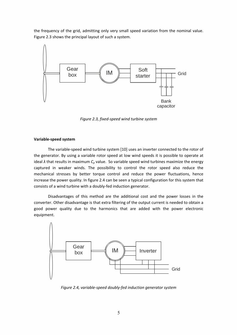
The variable‐speed wind turbine system [10] uses an inverter connected to the rotor of the generator. By using a variable rotor speed at low wind speeds it is possible to operate at ideal λ that results in maximum Cp value. So variable speed wind turbines maximize the energy captured in weaker winds. The possibility to control the rotor speed also reduce the mechanical stresses by better torque control and reduce the power fluctuations, hence increase the power quality. In figure 2.4 can be seen a typical configuration for this system that consists of a wind turbine with a doubly‐fed induction generator.

Disadvantages of this method are the additional cost and the power losses in the converter. Other disadvantage is that extra filtering of the output current is needed to obtain a good power quality due to the harmonics that are added with the power electronic equipment.

Gearbox IM

Grid

Inverter

Figure 2.4, variable‐speed doubly‐fed induction generator system

6

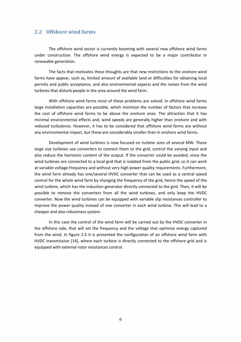
2.2 Offshore wind farms

The offshore wind sector is currently booming with several new offshore wind farms under construction. The offshore wind energy is expected to be a major contributor in renewable generation.

The facts that motivates these thoughts are that new restrictions to the onshore wind farms have appear, such as, limited amount of available land or difficulties for obtaining local permits and public acceptance, and also environmental aspects and the noises from the wind turbines that disturb people in the area around the wind farm.

With offshore wind farms most of these problems are solved. In offshore wind farms large installation capacities are possible, which minimize the number of factors that increase the cost of offshore wind farms to be above the onshore ones. The attraction that it has minimal environmental effects and, wind speeds are generally higher than onshore and with reduced turbulence. However, it has to be considered that offshore wind farms are without any environmental impact, but these are considerably smaller than in onshore wind farms.

Development of wind turbines is now focused on turbine sizes of several MW. These large size turbines use converters to connect them to the grid, control the varying input and also reduce the harmonic content of the output. If the converter could be avoided, since the wind turbines are connected to a local grid that is isolated from the public grid; so it can work at variable voltage‐frequency and without very high power quality requirements. Furthermore, the wind farm already has one/several HVDC converter that can be used as a central speed control for the whole wind farm by changing the frequency of the grid, hence the speed of the wind turbine, which has the induction generator directly connected to the grid. Then, it will be possible to remove the converters from all the wind turbines, and only keep the HVDC converter. Now the wind turbines can be equipped with variable slip resistances controller to improve the power quality instead of one converter in each wind turbine. This will lead to a cheaper and also robustness system.

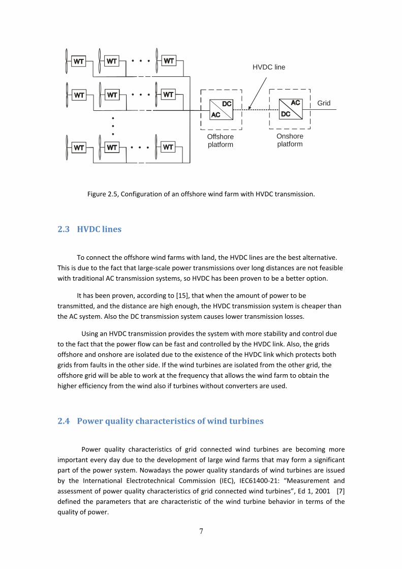
In this case the control of the wind farm will be carried out by the HVDC converter in the offshore side, that will set the frequency and the voltage that optimize energy captured from the wind. In figure 2.5 it is presented the configuration of an offshore wind farm with HVDC transmission [14], where each turbine is directly connected to the offshore grid and is equipped with external rotor resistances control.

7

Offshoreplatform

Onshoreplatform

HVDC line

Grid

Figure 2.5, Configuration of an offshore wind farm with HVDC transmission.

2.3 HVDC lines

To connect the offshore wind farms with land, the HVDC lines are the best alternative. This is due to the fact that large‐scale power transmissions over long distances are not feasible with traditional AC transmission systems, so HVDC has been proven to be a better option.

It has been proven, according to [15], that when the amount of power to be transmitted, and the distance are high enough, the HVDC transmission system is cheaper than the AC system. Also the DC transmission system causes lower transmission losses.

Using an HVDC transmission provides the system with more stability and control due to the fact that the power flow can be fast and controlled by the HVDC link. Also, the grids offshore and onshore are isolated due to the existence of the HVDC link which protects both grids from faults in the other side. If the wind turbines are isolated from the other grid, the offshore grid will be able to work at the frequency that allows the wind farm to obtain the higher efficiency from the wind also if turbines without converters are used.

2.4 Power quality characteristics of wind turbines

Power quality characteristics of grid connected wind turbines are becoming more important every day due to the development of large wind farms that may form a significant part of the power system. Nowadays the power quality standards of wind turbines are issued by the International Electrotechnical Commission (IEC), IEC61400‐21: “Measurement and assessment of power quality characteristics of grid connected wind turbines”, Ed 1, 2001 [7] defined the parameters that are characteristic of the wind turbine behavior in terms of the quality of power.

8

With the development of IEC61400‐21, it was possible to identify the factors and characteristics with highest influence on the power quality of wind turbines and the parameters then became more adapted to their quantification, to act as normalized quality indicators. These parameters are used to estimate the power quality of a wind turbine.

The typical behavior of a wind park based on induction generators directly connected to the grid, delivers a fairly variable power to the grid. This power flow can contribute to flicker emissions and affect the mean voltage profile. Certainly, this can be compensated by installation of reactive power compensation. The use of doubly‐fed induction generators or generators with fully rated frequency converters generally offers smaller fluctuations in the active power output. But the disadvantage of using power electronic converters may be a higher harmonic distortion, increased cost and losses in the converter

As mentioned before, the publication of the IEC 61400‐21 standard enabled the determination of systematic parameters to characterize the quality of power of grid connected wind turbines. In the chapter 5 “Evaluation of the controller”, improvement of the power quality that is achieved with the use of the variable rotor resistances controller will be determined. The main parameter that will be used for this purpose will be the flicker emission. This parameter gives an idea of the wind power fluctuations in steady‐state operation. Another parameter that can be used is the emission of current harmonics, but in this case the controller will have no effect on this parameter since it is not using power electronic converters that are the equipment that mostly is causing the current harmonics emission.

9

Chapter 3

Induction machine

In this chapter, a suitable model of an induction machine will be presented. Further, the linearization of the obtained model will be shown. At the end, it will be demonstrated how the induction machine behaves depending on the value of the rotor resistance.

3.1 Induction machine as wind turbine generator

The induction generators that are used in the wind turbine industry [12] have two main types of rotor: squirrel cage rotor or wound‐cage rotor. This last can have slip rings that can be connected to an external circuit. When it is desired to control the turbine, a wound rotor with slip rings has to be used.

The slip of an induction generator is usually very small (for efficiency reasons), but the slip depends on the resistance of the rotor windings. Thus, it is possible to increase the rotor resistance by increasing external resistances connected to the slip rings. The fact that the generator will increase or decrease its speed slightly if the torque varies is a very useful mechanical property; because this means less stresses in the gearbox and in the induction machine, so it will be possible to use smaller (accordingly cheaper) gearboxes.

Running wind turbine at variable speed has several advantages, one is that it allows the rotor to speed up while a wind gust is happening, storing the excess of energy into rotational energy until the wind dust is finished. In addition, the conversion of wind energy into shaft energy will increase if the wind turbine can operate at its optimal speed depending on the wind speed. Although, the complexity of the variable speed system leads to increased cost a reduced reliability due to use of power electronics and a more complicated control.

But new offshore wind farms connected to land through HVDC lines, open new possibilities regarding the local AC‐system which can be utilised in order to reduce the cost for a wind turbine system, and in addition increase the reliability. Removing the converter connected to the stator of the wind turbine is still possible to have variable rotor speed systems by changing the frequency of the offshore grid with the HVDC converter. Here is where the system with a variable rotor resistance system becomes of high interest.

10

3.2 Induction machine modelling

In this section, the equations that are needed to make a model of an induction machine will be presented. In this project only the induction machine model will be taken into account in the induction machine model, so the drive train will not be considered in the model of the induction machine where the controller will be tested.

The objective of this section is to transform the induction machine into a separately magnetized dc machine and presenting the mathematical model of it. The purpose of transforming the IM into a separately magnetized dc machine is to make the subsequent design of the controller easier. To make this transformation two steps are needed, first, make the Three‐phase to two‐phase transformation, and second transform from stationary to a rotating coordinate system oriented with the rotor flux in x‐direction.

To transform the three‐phase system into a two phase‐system the α‐β transformation will be done. The α‐β system will have two perpendicular axes, α and β, that can be considered as the real and complex axes in a complex plane. The interested reader can consult “Park transformation” [18] for further information.

The α‐β transformation is given by the following matrix for the amplitude invariant transformation:

1 0 00

√ √ (3.1)

The inverse two‐phase to three phase transformation is given by:

1 0√

√ (3.2)

Electrical dynamics

Now that the transformation needed to get the two‐phase system has been showed, the electrical equations that govern the dynamics of the stator and rotor of the induction machine in stationary coordinate systems will be stated below:

(3.3)

0 (3.4)

(3.5)

(3.6)

11

The equations above are the representation of dynamic model of the induction machine with a stationary coordinates (α‐β system), where is is the applied phase stator voltage to the induction machine, is the stator current, is the rotor current, is the stator flux, is the rotor flux, is the stator resistance, is the rotor resistance, is the stator inductance, is the rotor inductance, is the magnetizing inductance and is the rotor speed. The equations 3.3 to 3.6 will be used to create the model in MATLAB. From those equations is possible to derive the equivalent electrical circuit of the induction machine.

Rs

Rr

LrlLsl

LmUss

iss ir

s

Figure 3.1, dynamic induction machine model, T‐form

The circuit above these lines is called the T‐form, now it is possible to define:

(3.7)

(3.8)

Then, substituting these terms in the equations 3.5 and 3.6 and separating the quantities into real and imaginary parts, the electrical equations of the rotor and the stator become:

(3.9)

(3.10)

0 (3.11)

0 (3.12)

If we arrange these equations into the matrix form, the matrixes below will be obtained:

00

0 0 00 0 00

0

0 00 0

00 0

0

(3.13)

12

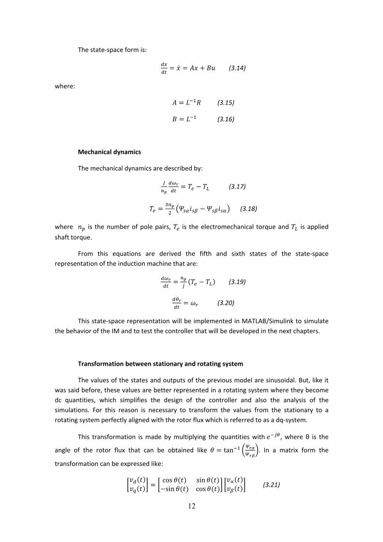
The state‐space form is:

(3.14)

where:

(3.15)

(3.16)

Mechanical dynamics

The mechanical dynamics are described by:

(3.17)

(3.18)

where is the number of pole pairs, is the electromechanical torque and is applied

shaft torque.

From this equations are derived the fifth and sixth states of the state‐space representation of the induction machine that are:

(3.19)

(3.20)

This state‐space representation will be implemented in MATLAB/Simulink to simulate the behavior of the IM and to test the controller that will be developed in the next chapters.

Transformation between stationary and rotating system

The values of the states and outputs of the previous model are sinusoidal. But, like it was said before, these values are better represented in a rotating system where they become dc quantities, which simplifies the design of the controller and also the analysis of the simulations. For this reason is necessary to transform the values from the stationary to a rotating system perfectly aligned with the rotor flux which is referred to as a dq‐system.

This transformation is made by multiplying the quantities with , where θ is the

angle of the rotor flux that can be obtained like tan . In a matrix form the

transformation can be expressed like:

cos sinsin cos (3.21)

13

and the inverse transformation will be:

cos sinsin cos (3.22)

The same matrixes 3.21 and 3.22 are used to transform the currents of the rotor and the stator from an α‐β system, into a dq‐system.

The mathematical equations can be also transformed and solved in a rotating reference frame. These equations are presented below.

(3.23)

0 (3.24)

(3.25)

(3.26)

(3.27)

(3.28)

where is the stator angular frequency.

These equations will be used in the next point to linearize the induction machine model, and to obtain the transfer functions that will be used to design the external rotor resistances controller.

Loss components in the induction generator

The losses in the induction machine mainly consist of two components, the copper losses and the iron losses, but here it will be only the copper losses considered. They occur in the stator and rotor windings, so increasing the rotor resistance will have an effect on them. The copper losses are determined as:

3 | | 3 |I | (3.29)

Where:

are the losses in the stator

are the losses in the rotor

14

3.3 Linearization of the induction machine model

Most of the existing theory for control system use linearized mathematical models of the process to control them in a closed‐loop manner. But in this case, the system is non linear, for this reason, it is needed to transform the non‐linear system into a linear one. Then the linearized model will be used in chapter 4 “Design of the controller for the extra rotor resistance” to develop the control system of the original non‐linear model.

A possible way to get a control system is the following: The first step is to obtain a non‐linear model of the system, like it was made in the previous section. Next the model is transformed into a linear one, as will be explained in this point. Later the control system is designed for the linear model. Finally, the controller is developed using the non‐linear model. The last two points will be explained in following chapters.

In this point it is presented how the linearization of the induction machine model described by nonlinear differential equations is performed. The procedure that will be used to linearize the equation system is based on Taylor’s series expansion [13].

The first step is to calculate the equilibrium point. The equilibrium points are those points where all the derivatives are simultaneously zero, and also the points which we are going to operate around with small variations. To find the equilibrium point the equation below has to be solved.

, 0 (3.30)

Once the equilibrium points have been calculated, the motion of the nonlinear system is in the neighborhood of the nominal system trajectory, that is:

∆ (3.31)

∆ (3.32)

where ∆ denotes small quantities. The new state must satisfy the equation 3.30 hence:

∆

∆ , ∆ (3.33)

The right‐hand side can be expanded into a Taylor series expansion, as follows:

∆

∆ , ∆

, ∆ ∆

∆ ∆ (3.34)

Since , 0, we have:

15

∆ ∆ ∆ ∆ ∆ (3.35)

Therefore, the linearized forms of equations 3.31 and 3.32 are

∆ ∆ ∆ (3.36)

∆ ∆ ∆ (3.37)

where the partial derivatives represent the Jacobian matrixes given by

…

… (3.38)

…

… (3.39)

∆ is the state vector of dimension n

∆ is the output vector of dimension m

∆ is the input vector of dimension r

A is the state matrix of size nxn

B is the input matrix of size nxr

C is the output matrix of size mxn

D is the proportion of input that appears directly in the output, size mxr

In this case, the system to be linearized is the dq‐model of the induction machine that has been presented in the equations 3.23 to 3.28. The states and the inputs of the system are:

Taking the equations 3.23 to 3.28 and rearranging the terms, the following equations to be linearized are obtained:

(3.40)

16

(3.41)

(3.42)

(3.43)

1.5 1.5 (3.44)

and according to equations 3.38 and 3.39, the A and B matrixes look like:

1.5 1.5 1.5 1.5 0

0

0

0

0

0

0

0

0

0

0

0

0

0

0

0 0

C is an mxn identity matrix, since the outputs that are of our interest are the same as the states of the model; and D is an mxr matrix of zeros because the outputs are not directly related with the inputs.

The above partial derivatives have to be evaluated at the equilibrium point about the system is being analyzed with small perturbation.

17

Transfer function

The transfer functions of the state‐space model showed before can be obtained by taking the Laplace transform of

∆ ∆ ∆ (3.45)

hence,

∆ ∆ ∆ (3.46)

Then, dividing by ∆ , giving

∆ ∆ (3.47)

∆ ∆ (3.48)

this is substituted for ∆ in the output equation 3.37 giving

∆ I A ∆ ∆ (3.49)

The definition of transfer function can be found as the ratio of the output to the input of a system,

∆ ∆⁄ (3.50)

and substituting the expression 3.49 in 3.50 gives

I A (3.51)

The dimension of the transfer function is mxr. Then, for every input there are n transfer functions, one for each state. In this case, there are 20 transfer function relating every state to every input of the system (4 inputs x 5 states = 20 transfer functions).

3.4 Induction machine with extra rotor resistance

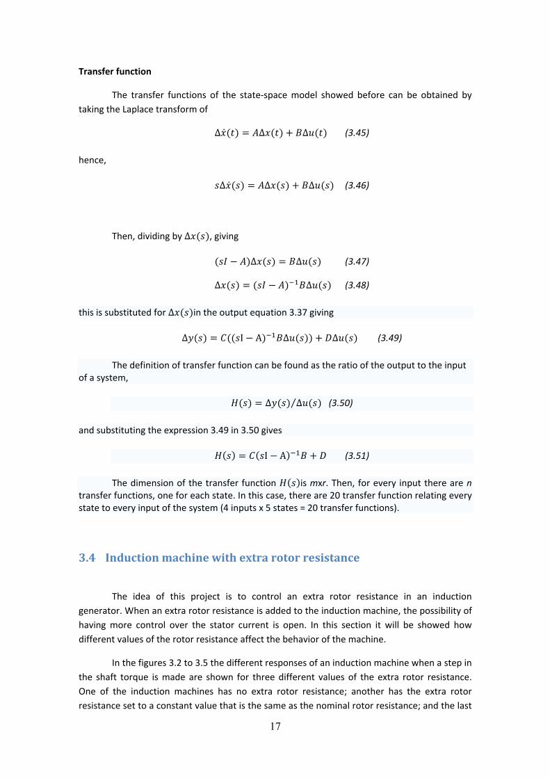
The idea of this project is to control an extra rotor resistance in an induction generator. When an extra rotor resistance is added to the induction machine, the possibility of having more control over the stator current is open. In this section it will be showed how different values of the rotor resistance affect the behavior of the machine.

In the figures 3.2 to 3.5 the different responses of an induction machine when a step in the shaft torque is made are shown for three different values of the extra rotor resistance. One of the induction machines has no extra rotor resistance; another has the extra rotor resistance set to a constant value that is the same as the nominal rotor resistance; and the last

18

one has the extra rotor resistance set to a constant value that is the double of the nominal rotor resistance.

Figure 3.2, response to a step in the shaft torque(black line); in colour torque generated by the induction machine for different values in the rotor resistance; in blue Rr is equal to the nominal value, in green the Rr is the double of the nominal Rr and in red the Rr is three times the value of

the nominal Rr.

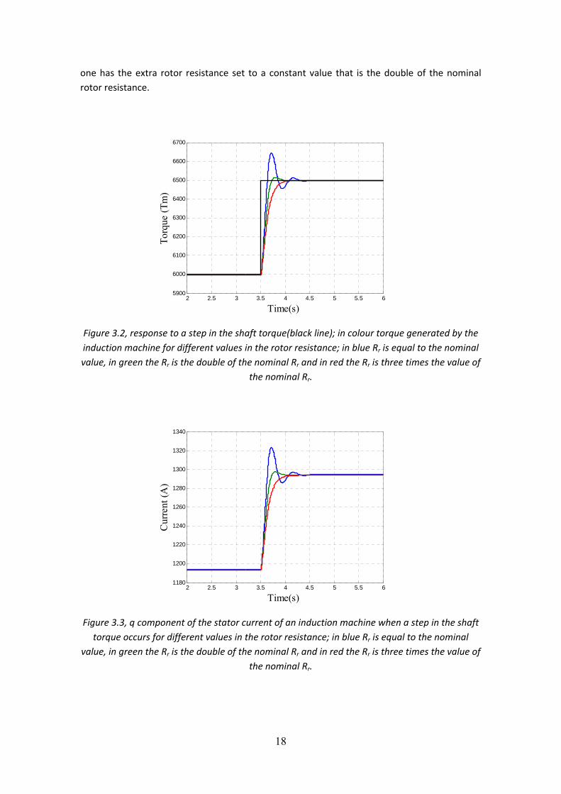
Figure 3.3, q component of the stator current of an induction machine when a step in the shaft torque occurs for different values in the rotor resistance; in blue Rr is equal to the nominal

value, in green the Rr is the double of the nominal Rr and in red the Rr is three times the value of the nominal Rr.

2 2.5 3 3.5 4 4.5 5 5.5 65900

6000

6100

6200

6300

6400

6500

6600

6700

Time(s)

Torq

ue (T

m)

2 2.5 3 3.5 4 4.5 5 5.5 61180

1200

1220

1240

1260

1280

1300

1320

1340

Time(s)

Cur

rent

(A)

19

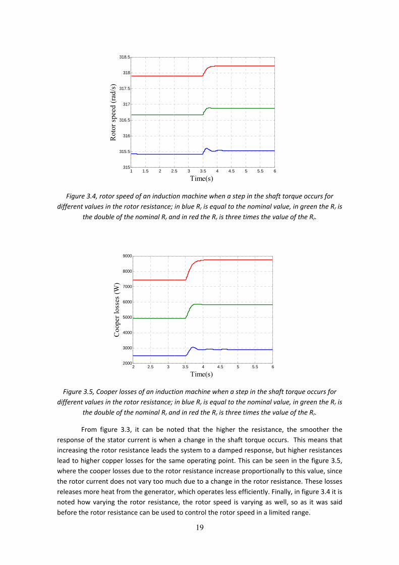
Figure 3.4, rotor speed of an induction machine when a step in the shaft torque occurs for different values in the rotor resistance; in blue Rr is equal to the nominal value, in green the Rr is

the double of the nominal Rr and in red the Rr is three times the value of the Rr.

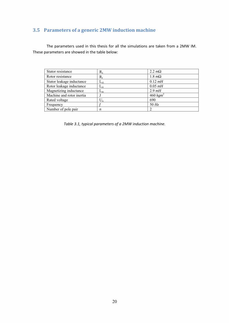
Figure 3.5, Cooper losses of an induction machine when a step in the shaft torque occurs for different values in the rotor resistance; in blue Rr is equal to the nominal value, in green the Rr is

the double of the nominal Rr and in red the Rr is three times the value of the Rr.

From figure 3.3, it can be noted that the higher the resistance, the smoother the response of the stator current is when a change in the shaft torque occurs. This means that increasing the rotor resistance leads the system to a damped response, but higher resistances lead to higher copper losses for the same operating point. This can be seen in the figure 3.5, where the cooper losses due to the rotor resistance increase proportionally to this value, since the rotor current does not vary too much due to a change in the rotor resistance. These losses releases more heat from the generator, which operates less efficiently. Finally, in figure 3.4 it is noted how varying the rotor resistance, the rotor speed is varying as well, so as it was said before the rotor resistance can be used to control the rotor speed in a limited range.

1 1.5 2 2.5 3 3.5 4 4.5 5 5.5 6315

315.5

316

316.5

317

317.5

318

318.5

Time(s)

Rot

or s

peed

(rad

/s)

2 2.5 3 3.5 4 4.5 5 5.5 62000

3000

4000

5000

6000

7000

8000

9000

Time(s)

Coo

per l

osse

s (W

)

20

3.5 Parameters of a generic 2MW induction machine

The parameters used in this thesis for all the simulations are taken from a 2MW IM. These parameters are showed in the table below:

Stator resistance Rs 2.2 mΩ Rotor resistance Rr 1.8 mΩ Stator leakage inductance Lsλ 0.12 mH Rotor leakage inductance Lrλ 0.05 mH Magnetizing inductance Lm 2.9 mH Machine and rotor inertia J 460 kgm2

Rated voltage Un 690 Frequency f 50 Hz Number of pole pair n 2

Table 3.1, typical parameters of a 2MW induction machine.

21

Chapter 4

Design of the controller for the extra rotor resistance

The purpose of controlling the rotor resistance is that fluctuations in the input shaft torque do not affect the power quality of the output signal and in addition reduce the torque fluctuations in the shaft of the wind turbine. These fluctuations of the input torque could be produce for gusts of wind. When a gust of wind occurs, the mechanical torque will increase; consequently the mechanical rotor speed will increase as well. If the rotor speed increase, the electrical torque will also increase and as a result the stator power will increase too. But, increasing the effective rotor resistance of the induction machine will also increase the slip of the induction machine and allow the rotor to speed up while the gust of wind is happening, so it will keep the rotor side current constant and hence the stator power constant.

4.1 Model of the linearized 2MW induction machine

In the section 3.3 “linearization of the induction machine”, it was explained how a linearized model of an induction machine could be obtained, in order to use it for the design of a controller. Following the steps given in that section and using MATLAB, a linearized model of a 2MW induction machine was created.

For the space‐state model of a linearized induction machine model, which was presented in section 3.3 “linearization of the induction machine”, there are 20 transfer functions, relating the five states of the model to the four inputs of the model. But only one of them is of interest for the design of the controller. This is the transfer function that links the variation in the q component of the stator current to the variation in the extra rotor resistance.

This is due to the fact that the extra rotor resistance is the only parameter that is possible to control (in a very small range), and the q component of the stator current is the parameter that will be used as reference for the control system, since the stator current is related with the power quality parameters.

After that, the non‐linear model and the linearized model of the induction machine were compared in order to see if they behave in a similar way, so that the linearized model could be used for the later develop of the controller. Both systems (non‐linear and linearized) were compared for a step in the extra rotor resistance and in the shaft torque, for different values of these steps.

22

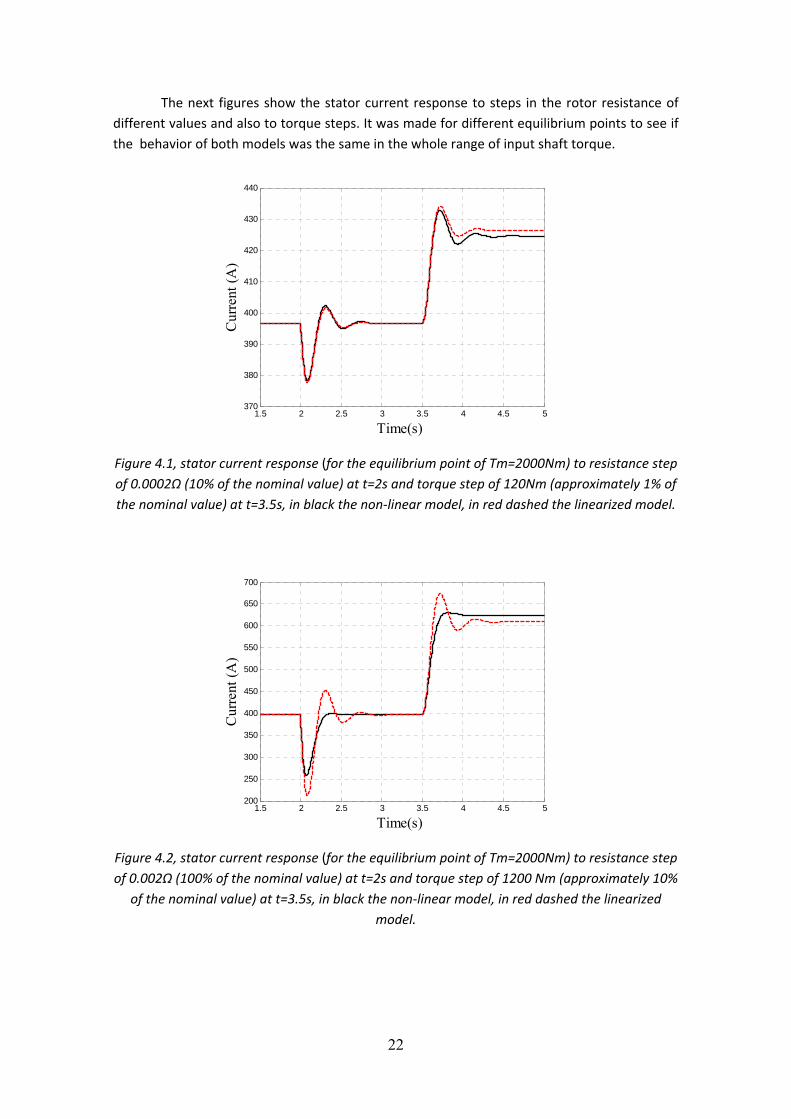
The next figures show the stator current response to steps in the rotor resistance of different values and also to torque steps. It was made for different equilibrium points to see if the behavior of both models was the same in the whole range of input shaft torque.

Figure 4.1, stator current response (for the equilibrium point of Tm=2000Nm) to resistance step of 0.0002Ω (10% of the nominal value) at t=2s and torque step of 120Nm (approximately 1% of the nominal value) at t=3.5s, in black the non‐linear model, in red dashed the linearized model.

Figure 4.2, stator current response (for the equilibrium point of Tm=2000Nm) to resistance step of 0.002Ω (100% of the nominal value) at t=2s and torque step of 1200 Nm (approximately 10%

of the nominal value) at t=3.5s, in black the non‐linear model, in red dashed the linearized model.

1.5 2 2.5 3 3.5 4 4.5 5370

380

390

400

410

420

430

440

Time(s)

Cur

rent

(A)

1.5 2 2.5 3 3.5 4 4.5 5200

250

300

350

400

450

500

550

600

650

700

Time(s)

Cur

rent

(A)

23

Figure 4.3, stator current response (for the equilibrium point of Tm=6000Nm) to resistance step of 0.0002Ω (10% of the nominal value) at t=2s and torque step of 120Nm (approximately 1% of the nominal value) at t=3.5s, in black the non‐linear model, in red dashed the linearized model.

Figure 4.4, stator current response (for the equilibrium point of Tm=6000Nm) to resistance step of 0.002Ω (100% of the nominal value) at t=2s and torque step of 1200 Nm (approximately 10%

of the nominal value) at t=3.5s, in black the non‐linear model, in red dashed the linearized model.

1.5 2 2.5 3 3.5 4 4.5 51130

1140

1150

1160

1170

1180

1190

1200

1210

1220

1230

Time(s)

Cur

rent

(A)

1.5 2 2.5 3 3.5 4 4.5 5600

700

800

900

1000

1100

1200

1300

1400

1500

Time(s)

Cur

rent

(A)

24

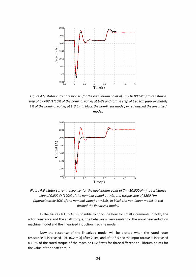
Figure 4.5, stator current response (for the equilibrium point of Tm=10.000 Nm) to resistance step of 0.0002 Ω (10% of the nominal value) at t=2s and torque step of 120 Nm (approximately 1% of the nominal value) at t=3.5s, in black the non‐linear model, in red dashed the linearized

model.

Figure 4.6, stator current response (for the equilibrium point of Tm=10.000 Nm) to resistance step of 0.002 Ω (100% of the nominal value) at t=2s and torque step of 1200 Nm

(approximately 10% of the nominal value) at t=3.5s, in black the non‐linear model, in red dashed the linearized model.

In the figures 4.1 to 4.6 is possible to conclude how for small increments in both, the rotor resistance and the shaft torque, the behavior is very similar for the non‐linear induction machine model and the linearized induction machine model.

Now the response of the linearized model will be plotted when the rated rotor resistance is increased 10% (0.2 mΩ) after 2 sec, and after 3.5 sec the input torque is increased a 10 % of the rated torque of the machine (1.2 kNm) for three different equilibrium points for the value of the shaft torque.

1.5 2 2.5 3 3.5 4 4.5 51900

1920

1940

1960

1980

2000

2020

2040

Time(s)

Cur

rent

(A)

1.5 2 2.5 3 3.5 4 4.5 51000

1200

1400

1600

1800

2000

2200

2400

Time(s)

Cur

rent

(A)

25

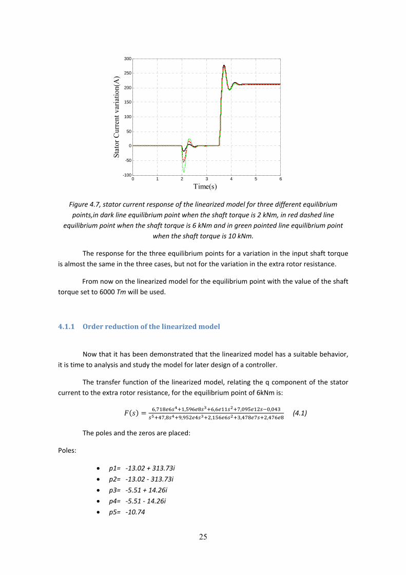
Figure 4.7, stator current response of the linearized model for three different equilibrium points,in dark line equilibrium point when the shaft torque is 2 kNm, in red dashed line

equilibrium point when the shaft torque is 6 kNm and in green pointed line equilibrium point when the shaft torque is 10 kNm.

The response for the three equilibrium points for a variation in the input shaft torque is almost the same in the three cases, but not for the variation in the extra rotor resistance.

From now on the linearized model for the equilibrium point with the value of the shaft torque set to 6000 Tm will be used.

4.1.1 Order reduction of the linearized model

Now that it has been demonstrated that the linearized model has a suitable behavior, it is time to analysis and study the model for later design of a controller.

The transfer function of the linearized model, relating the q component of the stator current to the extra rotor resistance, for the equilibrium point of 6kNm is:

, , , , ,, , , , ,

(4.1)

The poles and the zeros are placed:

Poles:

• p1= ‐13.02 + 313.73i

• p2= ‐13.02 ‐ 313.73i

• p3= ‐5.51 + 14.26i

• p4= ‐5.51 ‐ 14.26i

• p5= ‐10.74

0 1 2 3 4 5 6-100

-50

0

50

100

150

200

250

300

Time(s)

Stat

or C

urre

nt v

aria

tion(

A)

26

Zeros:

• z1= ‐6.5 + 313.73i

• z2= ‐6.5 ‐ 313.73i

• z3= ‐10.77

• z4= 0

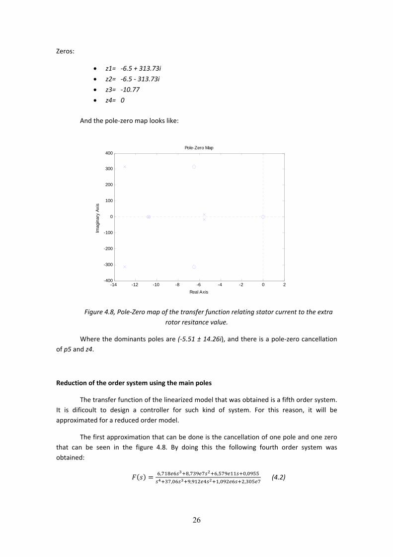
And the pole‐zero map looks like:

Figure 4.8, Pole‐Zero map of the transfer function relating stator current to the extra rotor resitance value.

Where the dominants poles are (‐5.51 ± 14.26i), and there is a pole‐zero cancellation of p5 and z4.

Reduction of the order system using the main poles

The transfer function of the linearized model that was obtained is a fifth order system. It is dificoult to design a controller for such kind of system. For this reason, it will be approximated for a reduced order model.

The first approximation that can be done is the cancellation of one pole and one zero that can be seen in the figure 4.8. By doing this the following fourth order system was obtained:

, , , ,, , , ,

(4.2)

-14 -12 -10 -8 -6 -4 -2 0 2-400

-300

-200

-100

0

100

200

300

400Pole-Zero Map

Real Axis

Imag

inar

y Ax

is

27

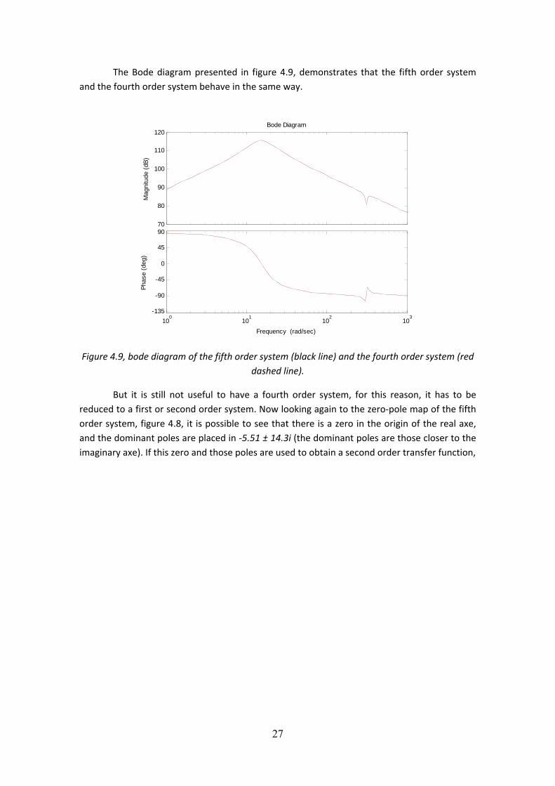
The Bode diagram presented in figure 4.9, demonstrates that the fifth order system and the fourth order system behave in the same way.

Figure 4.9, bode diagram of the fifth order system (black line) and the fourth order system (red dashed line).

But it is still not useful to have a fourth order system, for this reason, it has to be reduced to a first or second order system. Now looking again to the zero‐pole map of the fifth order system, figure 4.8, it is possible to see that there is a zero in the origin of the real axe, and the dominant poles are placed in ‐5.51 ± 14.3i (the dominant poles are those closer to the imaginary axe). If this zero and those poles are used to obtain a second order transfer function,

70

80

90

100

110

120

Mag

nitu

de (d

B)

100

101

102

103

-135

-90

-45

0

45

90

Phas

e (d

eg)

Bode Diagram

Frequency (rad/sec)

28

Figure 4.10, bode diagram of the fifth order system (black line) and the system using the dominant poles (red dashed line).

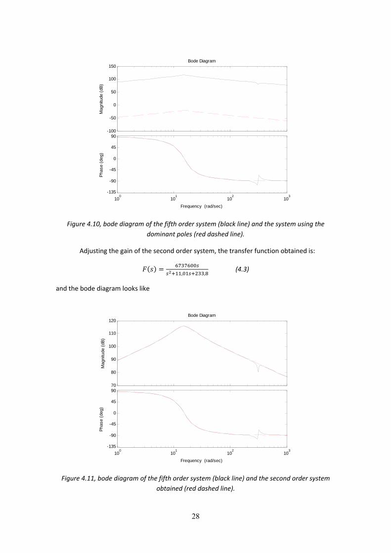
Adjusting the gain of the second order system, the transfer function obtained is:

, , (4.3)

and the bode diagram looks like

Figure 4.11, bode diagram of the fifth order system (black line) and the second order system obtained (red dashed line).

-100

-50

0

50

100

150

Mag

nitu

de (d

B)

100

101

102

103

-135

-90

-45

0

45

90

Phas

e (d

eg)

Bode Diagram

Frequency (rad/sec)

70

80

90

100

110

120

Mag

nitu

de (d

B)

100

101

102

103

-135

-90

-45

0

45

90

Phas

e (d

eg)

Bode Diagram

Frequency (rad/sec)

29

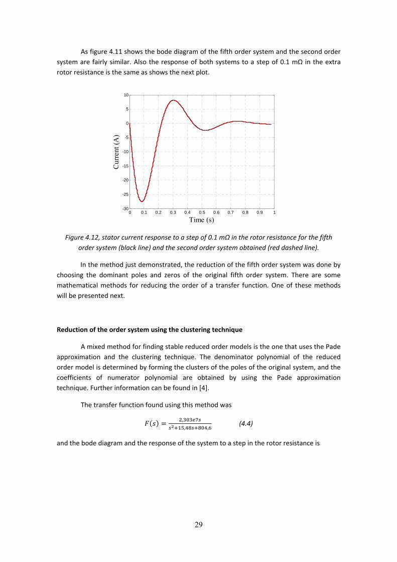
As figure 4.11 shows the bode diagram of the fifth order system and the second order system are fairly similar. Also the response of both systems to a step of 0.1 mΩ in the extra rotor resistance is the same as shows the next plot.

Figure 4.12, stator current response to a step of 0.1 mΩ in the rotor resistance for the fifth order system (black line) and the second order system obtained (red dashed line).

In the method just demonstrated, the reduction of the fifth order system was done by choosing the dominant poles and zeros of the original fifth order system. There are some mathematical methods for reducing the order of a transfer function. One of these methods will be presented next.

Reduction of the order system using the clustering technique

A mixed method for finding stable reduced order models is the one that uses the Pade approximation and the clustering technique. The denominator polynomial of the reduced order model is determined by forming the clusters of the poles of the original system, and the coefficients of numerator polynomial are obtained by using the Pade approximation technique. Further information can be found in [4].

The transfer function found using this method was

,, ,

(4.4)

and the bode diagram and the response of the system to a step in the rotor resistance is

0 0.1 0.2 0.3 0.4 0.5 0.6 0.7 0.8 0.9 1-30

-25

-20

-15

-10

-5

0

5

10

Time (s)

Cur

rent

(A)

30

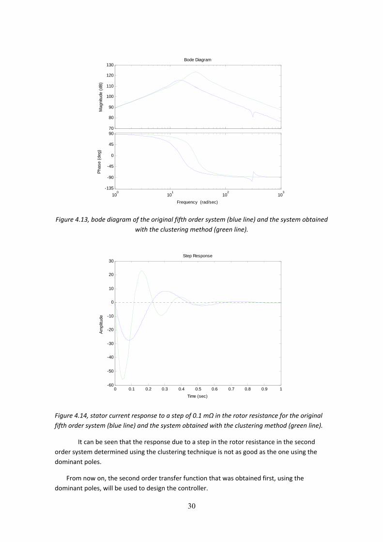
Figure 4.13, bode diagram of the original fifth order system (blue line) and the system obtained with the clustering method (green line).

Figure 4.14, stator current response to a step of 0.1 mΩ in the rotor resistance for the original fifth order system (blue line) and the system obtained with the clustering method (green line).

It can be seen that the response due to a step in the rotor resistance in the second order system determined using the clustering technique is not as good as the one using the dominant poles.

From now on, the second order transfer function that was obtained first, using the dominant poles, will be used to design the controller.

70

80

90

100

110

120

130

Mag

nitu

de (d

B)

100

101

102

103

-135

-90

-45

0

45

90

Phas

e (d

eg)

Bode Diagram

Frequency (rad/sec)

0 0.1 0.2 0.3 0.4 0.5 0.6 0.7 0.8 0.9 1-60

-50

-40

-30

-20

-10

0

10

20

30Step Response

Time (sec)

Ampl

itude

31

4.2 Design of the controller

The idea behind the controller is to high‐pass filter the q component of the stator current, to obtain the high‐pass frequency components of the signal, the part that is pursued to eliminate.

Gearbox IM

Powerelectronics

Grid

External rotorresistances

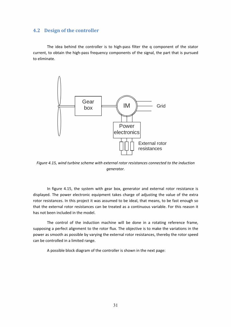
Figure 4.15, wind turbine scheme with external rotor resistances connected to the induction generator.

In figure 4.15, the system with gear box, generator and external rotor resistance is displayed. The power electronic equipment takes charge of adjusting the value of the extra rotor resistances. In this project it was assumed to be ideal, that means, to be fast enough so that the external rotor resistances can be treated as a continuous variable. For this reason it has not been included in the model.

The control of the induction machine will be done in a rotating reference frame, supposing a perfect alignment to the rotor flux. The objective is to make the variations in the power as smooth as possible by varying the external rotor resistances, thereby the rotor speed can be controlled in a limited range.

A possible block diagram of the controller is shown in the next page:

32

Controller InductionMachine

High-passFilter

isqref

isqRR

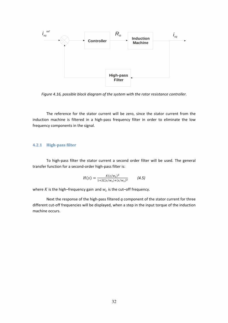
Figure 4.16, possible block diagram of the system with the rotor resistance controller.

The reference for the stator current will be zero, since the stator current from the induction machine is filtered in a high‐pass frequency filter in order to eliminate the low frequency components in the signal.

4.2.1 High­pass filter

To high‐pass filter the stator current a second order filter will be used. The general transfer function for a second‐order high‐pass filter is:

⁄⁄ ⁄ (4.5)

where is the high–frequency gain and is the cut–off frequency.

Next the response of the high‐pass filtered q component of the stator current for three different cut‐off frequencies will be displayed, when a step in the input torque of the induction machine occurs.

33

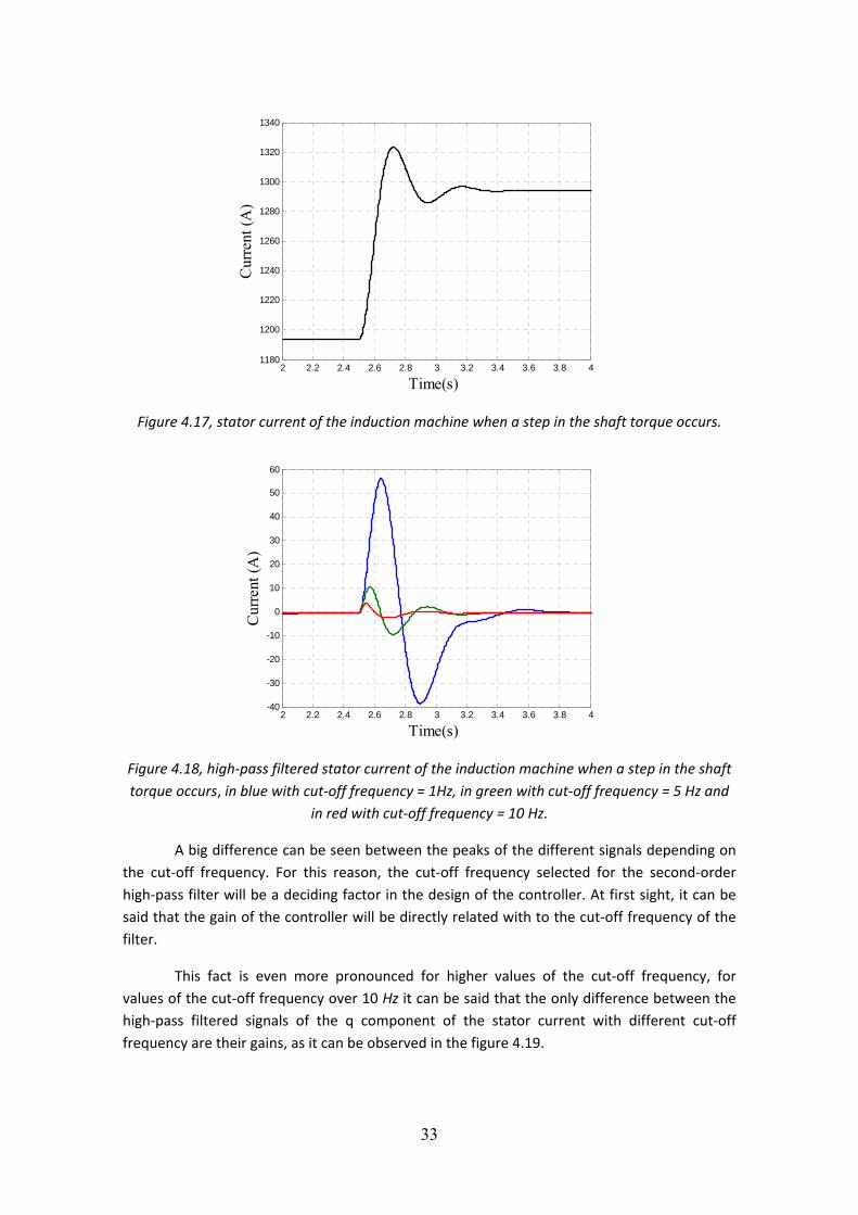
Figure 4.17, stator current of the induction machine when a step in the shaft torque occurs.

Figure 4.18, high‐pass filtered stator current of the induction machine when a step in the shaft torque occurs, in blue with cut‐off frequency = 1Hz, in green with cut‐off frequency = 5 Hz and

in red with cut‐off frequency = 10 Hz.

A big difference can be seen between the peaks of the different signals depending on the cut‐off frequency. For this reason, the cut‐off frequency selected for the second‐order high‐pass filter will be a deciding factor in the design of the controller. At first sight, it can be said that the gain of the controller will be directly related with to the cut‐off frequency of the filter.

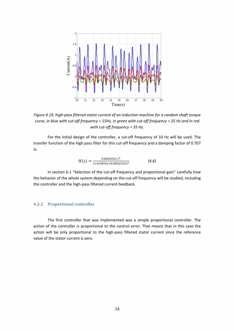
This fact is even more pronounced for higher values of the cut‐off frequency, for values of the cut‐off frequency over 10 Hz it can be said that the only difference between the high‐pass filtered signals of the q component of the stator current with different cut‐off frequency are their gains, as it can be observed in the figure 4.19.

2 2.2 2.4 2.6 2.8 3 3.2 3.4 3.6 3.8 41180

1200

1220

1240

1260

1280

1300

1320

1340

Time(s)

Cur

rent

(A)

2 2.2 2.4 2.6 2.8 3 3.2 3.4 3.6 3.8 4-40

-30

-20

-10

0

10

20

30

40

50

60

Time(s)

Cur

rent

(A)

34

Figure 4.19, high‐pass filtered stator current of an induction machine for a random shaft torque curve, in blue with cut‐off frequency = 15Hz, in green with cut‐off frequency = 25 Hz and in red

with cut‐off frequency = 35 Hz.

For the initial design of the controller, a cut‐off frequency of 10 Hz will be used. The transfer function of the high pass filter for this cut‐off frequency and a damping factor of 0.707 is:

. . .

(4.6)

In section 6.1 “Selection of the cut‐off frequency and proportional gain” carefully how the behavior of the whole system depending on the cut‐off frequency will be studied, including the controller and the high‐pass filtered current feedback.

4.2.2 Proportional controller

The first controller that was implemented was a simple proportional controller. The action of the controller is proportional to the control error. That means that in this case the action will be only proportional to the high‐pass filtered stator current since the reference value of the stator current is zero.

10 11 12 13 14 15 16 17 18 19 20-1

-0.5

0

0.5

1

1.5

2

Time(s)

Cur

rent

(A)

35

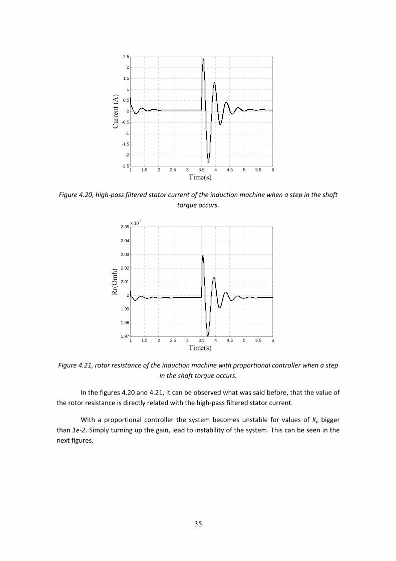
Figure 4.20, high‐pass filtered stator current of the induction machine when a step in the shaft torque occurs.

Figure 4.21, rotor resistance of the induction machine with proportional controller when a step in the shaft torque occurs.

In the figures 4.20 and 4.21, it can be observed what was said before, that the value of the rotor resistance is directly related with the high‐pass filtered stator current.

With a proportional controller the system becomes unstable for values of Kp bigger than 1e‐2. Simply turning up the gain, lead to instability of the system. This can be seen in the next figures.

1 1.5 2 2.5 3 3.5 4 4.5 5 5.5 6-2.5

-2

-1.5

-1

-0.5

0

0.5

1

1.5

2

2.5

Time(s)

Cur

rent

(A)

1 1.5 2 2.5 3 3.5 4 4.5 5 5.5 61.97

1.98

1.99

2

2.01

2.02

2.03

2.04

2.05x 10-3

Time(s)

Rr(O

mh)

36

Figure 4.22, stator current of the induction machine when a step of 500 Nm is introduce at t = 3,5 sec, in black the response of the system with a proportional controller(Kp=1e‐8). The red

dashed line is the response of the system without controller.

Figure 4.23, stator current of the induction machine when a step of 500 Nm is introduce at t = 3,5 sec, in black the response of the system with a proportional controller(kp=1e‐5). The red

dashed line is the response of the system without controller.

For higher values of Kp the system is becoming more and more unstable until it is critically stable for Kp = 1e‐2. This can be explained by studying the next figures.

1 1.5 2 2.5 3 3.5 4 4.5 5 5.5 61180

1200

1220

1240

1260

1280

1300

1320

1340

Time(s)

Cur

rent

(A)

1 1.5 2 2.5 3 3.5 4 4.5 5 5.5 61180

1200

1220

1240

1260

1280

1300

1320

1340

Time(s)

Cur

rent

(A)

37

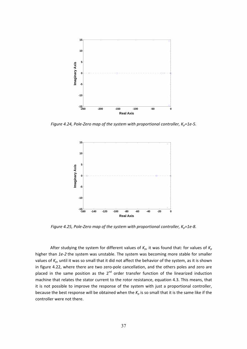
Figure 4.24, Pole‐Zero map of the system with proportional controller, Kp=1e‐5.

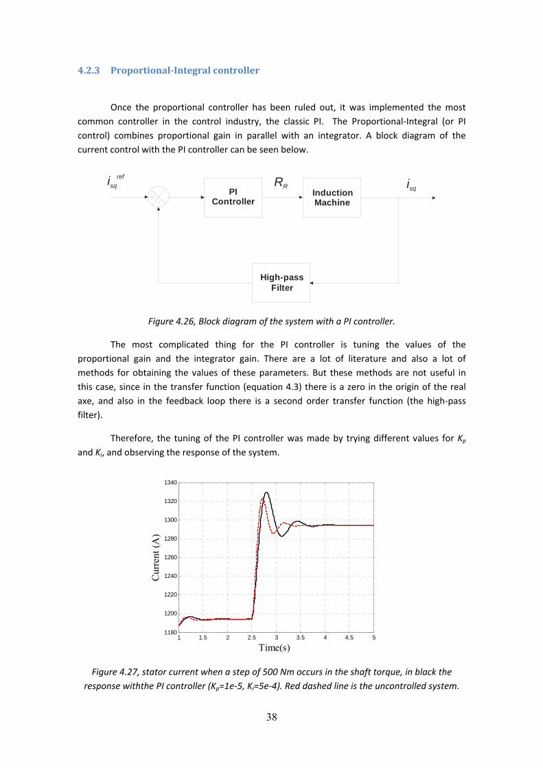
Figure 4.25, Pole‐Zero map of the system with proportional controller, Kp=1e‐8.

After studying the system for different values of Kp, it was found that: for values of Kp higher than 1e‐2 the system was unstable. The system was becoming more stable for smaller values of Kp, until it was so small that it did not affect the behavior of the system, as it is shown in figure 4.22, where there are two zero‐pole cancellation, and the others poles and zero are placed in the same position as the 2nd order transfer function of the linearized induction machine that relates the stator current to the rotor resistance, equation 4.3. This means, that it is not possible to improve the response of the system with just a proportional controller, because the best response will be obtained when the Kp is so small that it is the same like if the controller were not there.

-250 -200 -150 -100 -50 0-15

-10

-5

0

5

10

15

Real Axis

Imag

inar

y A

xis

-160 -140 -120 -100 -80 -60 -40 -20 0-15

-10

-5

0

5

10

15

Real Axis

Imag

inar

y A

xis

38

4.2.3 Proportional­Integral controller

Once the proportional controller has been ruled out, it was implemented the most common controller in the control industry, the classic PI. The Proportional‐Integral (or PI control) combines proportional gain in parallel with an integrator. A block diagram of the current control with the PI controller can be seen below.

PIController

InductionMachine

High-passFilter

isqref

isqRR

Figure 4.26, Block diagram of the system with a PI controller.

The most complicated thing for the PI controller is tuning the values of the proportional gain and the integrator gain. There are a lot of literature and also a lot of methods for obtaining the values of these parameters. But these methods are not useful in this case, since in the transfer function (equation 4.3) there is a zero in the origin of the real axe, and also in the feedback loop there is a second order transfer function (the high‐pass filter).

Therefore, the tuning of the PI controller was made by trying different values for Kp and Ki, and observing the response of the system.

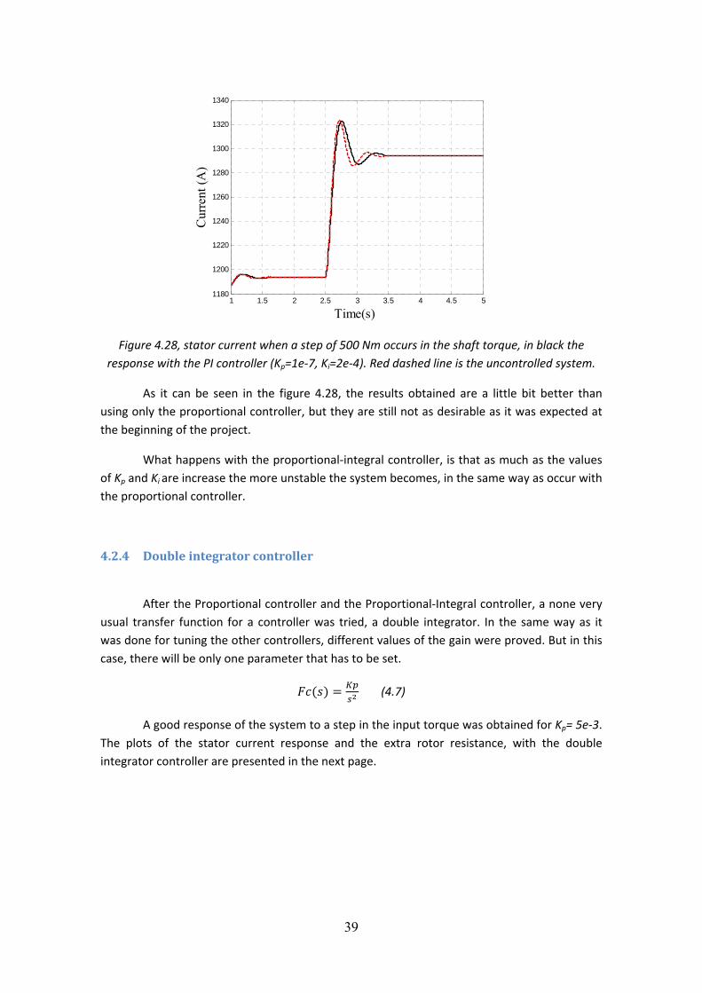
Figure 4.27, stator current when a step of 500 Nm occurs in the shaft torque, in black the response withthe PI controller (Kp=1e‐5, Ki=5e‐4). Red dashed line is the uncontrolled system.

1 1.5 2 2.5 3 3.5 4 4.5 51180

1200

1220

1240

1260

1280

1300

1320

1340

Time(s)

Cur

rent

(A)

39

Figure 4.28, stator current when a step of 500 Nm occurs in the shaft torque, in black the response with the PI controller (Kp=1e‐7, Ki=2e‐4). Red dashed line is the uncontrolled system.

As it can be seen in the figure 4.28, the results obtained are a little bit better than using only the proportional controller, but they are still not as desirable as it was expected at the beginning of the project.

What happens with the proportional‐integral controller, is that as much as the values of Kp and Ki are increase the more unstable the system becomes, in the same way as occur with the proportional controller.

4.2.4 Double integrator controller

After the Proportional controller and the Proportional‐Integral controller, a none very usual transfer function for a controller was tried, a double integrator. In the same way as it was done for tuning the other controllers, different values of the gain were proved. But in this case, there will be only one parameter that has to be set.

(4.7)

A good response of the system to a step in the input torque was obtained for Kp= 5e‐3. The plots of the stator current response and the extra rotor resistance, with the double integrator controller are presented in the next page.

1 1.5 2 2.5 3 3.5 4 4.5 51180

1200

1220

1240

1260

1280

1300

1320

1340

Time(s)

Cur

rent

(A)

40

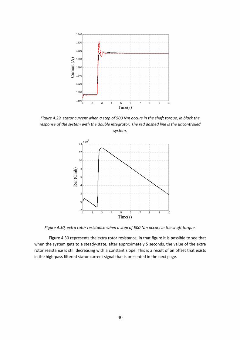
Figure 4.29, stator current when a step of 500 Nm occurs in the shaft torque, in black the response of the system with the double integrator. The red dashed line is the uncontrolled

system.

Figure 4.30, extra rotor resistance when a step of 500 Nm occurs in the shaft torque.

Figure 4.30 represents the extra rotor resistance, in that figure it is possible to see that when the system gets to a steady‐state, after approximately 5 seconds, the value of the extra rotor resistance is still decreasing with a constant slope. This is a result of an offset that exists in the high‐pass filtered stator current signal that is presented in the next page.

1 2 3 4 5 6 7 8 9 101180

1200

1220

1240

1260

1280

1300

1320

1340

Time(s)

Cur

rent

(A)

1 2 3 4 5 6 7 8 9 10-2

0

2

4

6

8

10

12

14x 10

-5

Time(s)

Rer

(Om

h)

41

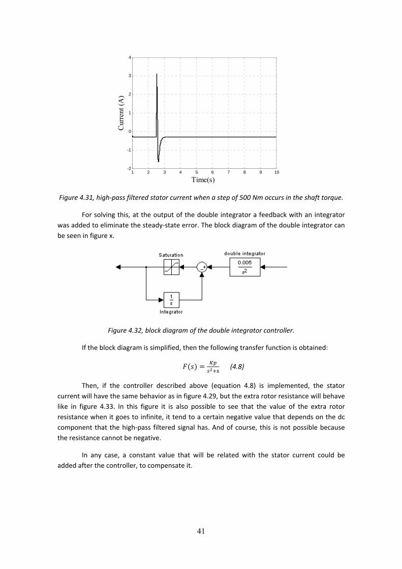
Figure 4.31, high‐pass filtered stator current when a step of 500 Nm occurs in the shaft torque.

For solving this, at the output of the double integrator a feedback with an integrator was added to eliminate the steady‐state error. The block diagram of the double integrator can be seen in figure x.

Figure 4.32, block diagram of the double integrator controller.

If the block diagram is simplified, then the following transfer function is obtained:

(4.8)

Then, if the controller described above (equation 4.8) is implemented, the stator current will have the same behavior as in figure 4.29, but the extra rotor resistance will behave like in figure 4.33. In this figure it is also possible to see that the value of the extra rotor resistance when it goes to infinite, it tend to a certain negative value that depends on the dc component that the high‐pass filtered signal has. And of course, this is not possible because the resistance cannot be negative.

In any case, a constant value that will be related with the stator current could be added after the controller, to compensate it.

1 2 3 4 5 6 7 8 9 10-2

-1

0

1

2

3

4

Time(s)

Cur

rent

(A)

42

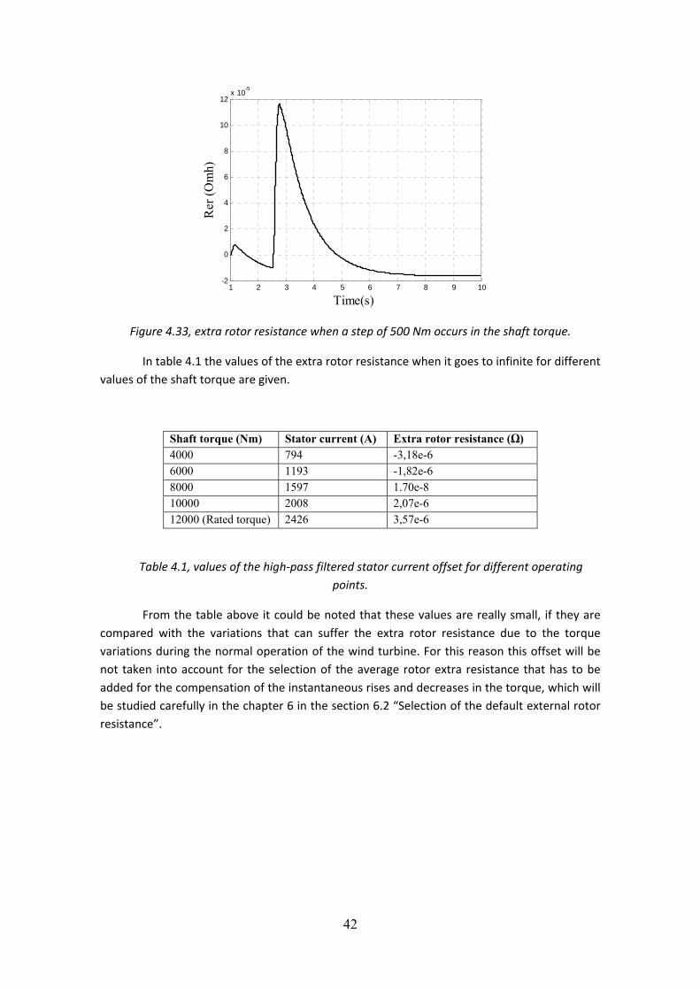
Figure 4.33, extra rotor resistance when a step of 500 Nm occurs in the shaft torque.

In table 4.1 the values of the extra rotor resistance when it goes to infinite for different values of the shaft torque are given.

Shaft torque (Nm) Stator current (A) Extra rotor resistance (Ω) 4000 794 -3,18e-6 6000 1193 -1,82e-6 8000 1597 1.70e-8 10000 2008 2,07e-6 12000 (Rated torque) 2426 3,57e-6

Table 4.1, values of the high‐pass filtered stator current offset for different operating points.

From the table above it could be noted that these values are really small, if they are compared with the variations that can suffer the extra rotor resistance due to the torque variations during the normal operation of the wind turbine. For this reason this offset will be not taken into account for the selection of the average rotor extra resistance that has to be added for the compensation of the instantaneous rises and decreases in the torque, which will be studied carefully in the chapter 6 in the section 6.2 “Selection of the default external rotor resistance”.

1 2 3 4 5 6 7 8 9 10-2

0

2

4

6

8

10

12x 10-5

Time(s)

Rer

(Om

h)

43

Chapter 5

Evaluation of the controller

The stator current controller that was developed in the previous chapter has been implemented in Matlab/Simulink to see the response of the whole system and analyze the power quality improvement as well as the mechanical stresses reduction. In this chapter, first the behavior of the system when it was exposed to synthetic shaft torque curves will be presented. After that, the response of the controlled system when it was exposed to real shaft torque data will be shown.

In this chapter, the values selected for the parameters to be tuned in the controlled system were Kp= 5e‐3 for the controller gain, a cut‐off frequency of 10 Hz for the high‐pass filter and a average value of 1.2 mΩ for the external rotor resistance. These values were proved to work fairly well for different shaft torque curves. In the next chapter it will be presented how different combinations of these parameters affect the behavior of the system.

5.1 Response of the system to synthetic curves

In the previous chapter it was shown how a step in the load torque affects the response of the IM with the stator current controller. In this section the response of the system for different synthetic load torque curves will be analyzed.

Response to stepped signal

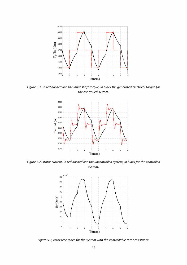
First the controller was analyzed with a signal where a step of 400 Nm occurs every second, to see if the system can follow positive load torque variations as well as negative. The electrical torque generated, the stator current and the rotor resistance are presented in the next page.

44

Figure 5.1, in red dashed line the input shaft torque, in black the generated electrical torque for the controlled system.

Figure 5.2, stator current, in red dashed line the uncontrolled system, in black for the controlled system.

Figure 5.3, rotor resistance for the system with the controllable rotor resistance.

1 2 3 4 5 6 7 8 9 105300

5400

5500

5600

5700

5800

5900

6000

6100

Time(s)

Tg,T

s (N

m)

1 2 3 4 5 6 7 8 9 101040

1060

1080

1100

1120

1140

1160

1180

1200

1220

Time(s)

Cur

rent

(A)

1 2 3 4 5 6 7 8 9 101.8

2

2.2

2.4

2.6

2.8

3

3.2

3.4

3.6

3.8x 10-3

Time(s)

Rr(O

mh)

45

From figure 5.2 it can be seen that the response of the controlled system is smother than the system without controller. It also can be noted that the overshoots that exist in the non‐controlled system are eliminated. Finally it can be mentioned that the control system follow a positive variation in the shaft torque as well as a negative.

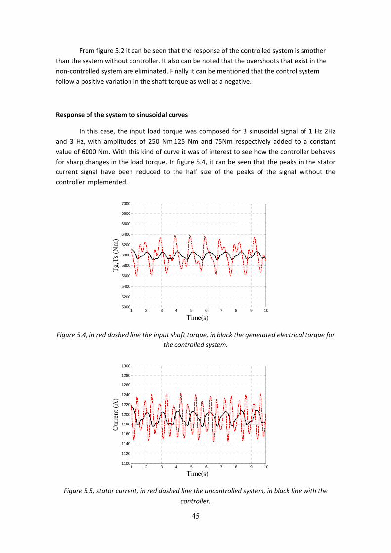
Response of the system to sinusoidal curves

In this case, the input load torque was composed for 3 sinusoidal signal of 1 Hz 2Hz and 3 Hz, with amplitudes of 250 Nm 125 Nm and 75Nm respectively added to a constant value of 6000 Nm. With this kind of curve it was of interest to see how the controller behaves for sharp changes in the load torque. In figure 5.4, it can be seen that the peaks in the stator current signal have been reduced to the half size of the peaks of the signal without the controller implemented.

Figure 5.4, in red dashed line the input shaft torque, in black the generated electrical torque for the controlled system.

Figure 5.5, stator current, in red dashed line the uncontrolled system, in black line with the controller.

1 2 3 4 5 6 7 8 9 105000

5200

5400

5600

5800

6000

6200

6400

6600

6800

7000

Time(s)

Tg,T

s (N

m)

1 2 3 4 5 6 7 8 9 101100

1120

1140

1160

1180

1200

1220

1240

1260

1280

1300

Time(s)

Cur

rent

(A)

46

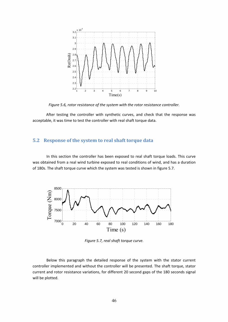
Figure 5.6, rotor resistance of the system with the rotor resistance controller.

After testing the controller with synthetic curves, and check that the response was acceptable, it was time to test the controller with real shaft torque data.

5.2 Response of the system to real shaft torque data

In this section the controller has been exposed to real shaft torque loads. This curve was obtained from a real wind turbine exposed to real conditions of wind, and has a duration of 180s. The shaft torque curve which the system was tested is shown in figure 5.7.

Figure 5.7, real shaft torque curve.

Below this paragraph the detailed response of the system with the stator current controller implemented and without the controller will be presented. The shaft torque, stator current and rotor resistance variations, for different 20 second gaps of the 180 seconds signal will be plotted.

1 2 3 4 5 6 7 8 9 102.2

2.3

2.4

2.5

2.6

2.7

2.8

2.9

3

3.1

3.2x 10-3

Time(s)

Rr(O

mh)

0 20 40 60 80 100 120 140 160 1807000

7500

8000

8500

Time (s)

Torq

ue (N

m)

47

’

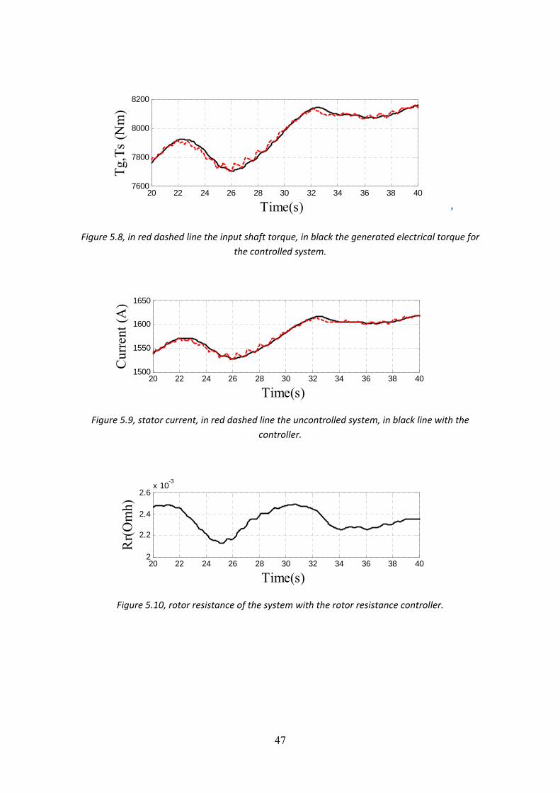
Figure 5.8, in red dashed line the input shaft torque, in black the generated electrical torque for the controlled system.

Figure 5.9, stator current, in red dashed line the uncontrolled system, in black line with the controller.

Figure 5.10, rotor resistance of the system with the rotor resistance controller.

20 22 24 26 28 30 32 34 36 38 407600

7800

8000

8200

Time(s)

Tg,T

s (N

m)

20 22 24 26 28 30 32 34 36 38 401500

1550

1600

1650

Time(s)

Cur

rent

(A)

20 22 24 26 28 30 32 34 36 38 402

2.2

2.4

2.6x 10-3

Time(s)

Rr(O

mh)

48

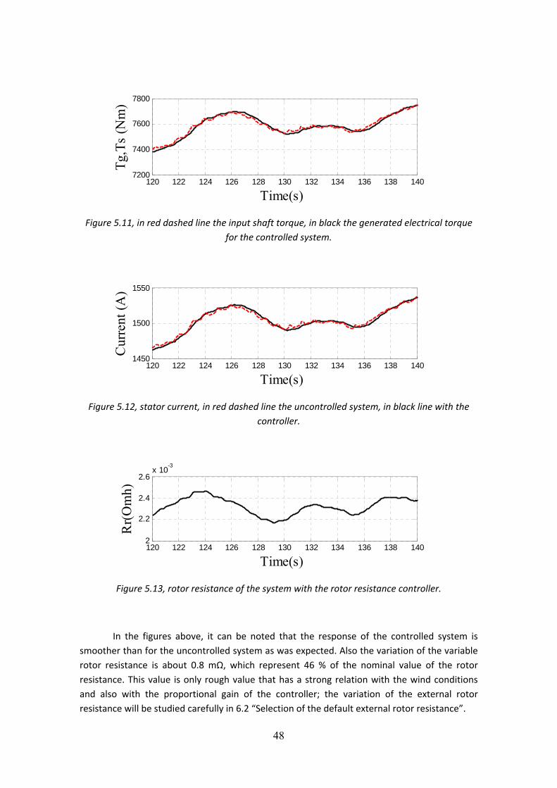
Figure 5.11, in red dashed line the input shaft torque, in black the generated electrical torque for the controlled system.

Figure 5.12, stator current, in red dashed line the uncontrolled system, in black line with the controller.

Figure 5.13, rotor resistance of the system with the rotor resistance controller.

In the figures above, it can be noted that the response of the controlled system is smoother than for the uncontrolled system as was expected. Also the variation of the variable rotor resistance is about 0.8 mΩ, which represent 46 % of the nominal value of the rotor resistance. This value is only rough value that has a strong relation with the wind conditions and also with the proportional gain of the controller; the variation of the external rotor resistance will be studied carefully in 6.2 “Selection of the default external rotor resistance”.

120 122 124 126 128 130 132 134 136 138 1407200

7400

7600

7800

Time(s)

Tg,T

s (N

m)

120 122 124 126 128 130 132 134 136 138 1401450

1500

1550

Time(s)

Cur

rent

(A)

120 122 124 126 128 130 132 134 136 138 1402

2.2

2.4

2.6x 10-3

Time(s)

Rr(O

mh)

49

The figures above are just illustrative, the developed controller will be analyzed carefully in the next section by measuring different parameters such as the flicker emission or the losses in the induction machine.

5.2.1 Flicker reduction

As it was said in the section 2.4 “Power quality characteristics of wind turbines”, one way of evaluate the power quality is measuring the flicker contribution of the wind turbine to the grid. The flicker contribution can be described with the dimensionless parameters Pst and Plt. The first one is referred to the short‐term influence, and the second one to the long term influence. In this case only the short‐term influence will be studied.

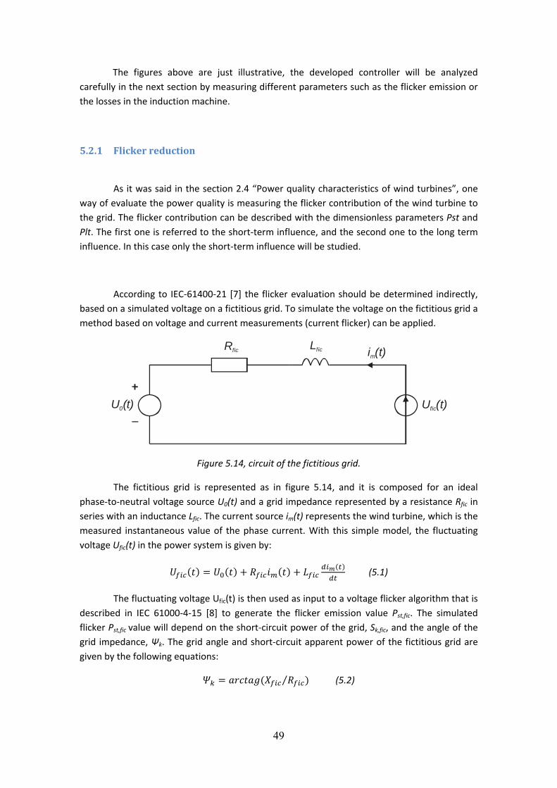
According to IEC‐61400‐21 [7] the flicker evaluation should be determined indirectly, based on a simulated voltage on a fictitious grid. To simulate the voltage on the fictitious grid a method based on voltage and current measurements (current flicker) can be applied.

U (t)0

i (t)mRfic Lfic

U (t)fic

Figure 5.14, circuit of the fictitious grid.

The fictitious grid is represented as in figure 5.14, and it is composed for an ideal phase‐to‐neutral voltage source U0(t) and a grid impedance represented by a resistance Rfic in series with an inductance Lfic. The current source im(t) represents the wind turbine, which is the measured instantaneous value of the phase current. With this simple model, the fluctuating voltage Ufic(t) in the power system is given by:

(5.1)

The fluctuating voltage Ufic(t) is then used as input to a voltage flicker algorithm that is described in IEC 61000‐4‐15 [8] to generate the flicker emission value Pst,fic. The simulated flicker Pst,fic value will depend on the short‐circuit power of the grid, Sk,fic, and the angle of the grid impedance, Ψk. The grid angle and short‐circuit apparent power of the fictitious grid are given by the following equations:

⁄ (5.2)

50

, (5.3)

for each Pst,fic value, a flicker coefficient c(Ψk) could be determined by utilizing:

,, (5.4)

In this project, the c(Ψk) value has been calculated on a fictive grid with a short‐circuit power of 50 times the rated power of the WT, as IEC‐61400‐21 recommends. Furthermore, an X/R ratio of 0.5 has been chosen. Then 26,565 .

The results of the c(Ψk) values for the stator current controller are presented in table 5.1. In the table appear different values for different gaps of 60 second from real shaft torque data.

The results of the stator current controller has been compared with the same system without any controller, with the rotor resistance value set to the double of the nominal rotor resistance, and with the system with a fixed rotor resistance set to three times the nominal value of the rotor resistance.

1st gap 2nd gap 3rd gap 4th gap 5th gap With stator current controller 0,48 0,4 0,41 0,335 0,395Without controller

0,895 0,575 0,585 0,52 0,59Fixed rotor resistance to 3.6 mΩ 0,69 0,475 0,495 0,415 0,5Fixed rotor resistance to 5.4 mΩ 0,61 0,44 0,46 0,385 0,46

Table 5.1, c(Ψk) values for different shaft torque curves

According to table 5.1, the power quality of the controlled system is better than in any other system studied. This is because the controlled system has the lower c(Ψk) values in the table. The reduction in the flicker contribution can go from 35% to more than 60% with regard to the uncontrolled system, depending on the shaft torque curves. If the average c(Ψk) is calculated for all the gaps, then the following results are obtained:

• With controller: c(Ψk) = 0,395

• Without controller: c(Ψk) = 0,675

• Fixed rotor resistance to 3.6 mΩ: c(Ψk) = 0,525

• Fixed rotor resistance to 5.4 mΩ: c(Ψk) = 0,48

The finding is that the average reduction of the flicker contribution by utilizing the controller is almost the 50% with regard to the uncontrolled system, for this shaft torque curves. The system with the rotor resistance fixed to three times the nominal rotor resistance

51

(5.4 mΩ) has the closest response to the controlled system. But as it was said before, the higher the rotor resistance is, the higher the losses in the rotor resistance will be. Later the losses in the machine will be studied in its own section.

It must be said that since the external rotor resistance can only vary in a small range, the reduction in the flicker contribution will be very dependent on the shaft torque curves, a higher reduction on the flicker emission was observed for a higher turbulence in the wind.

5.2.2 Mechanical stresses reduction

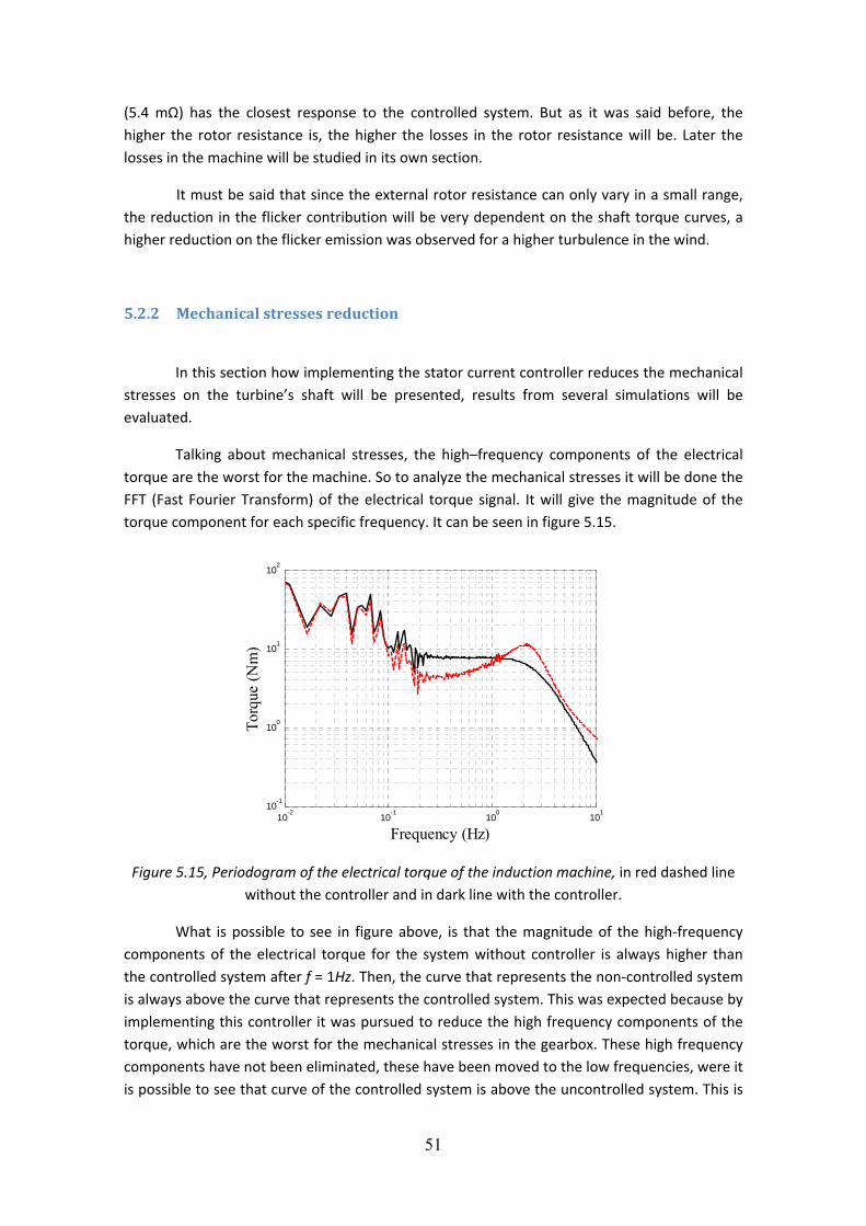
In this section how implementing the stator current controller reduces the mechanical stresses on the turbine’s shaft will be presented, results from several simulations will be evaluated.

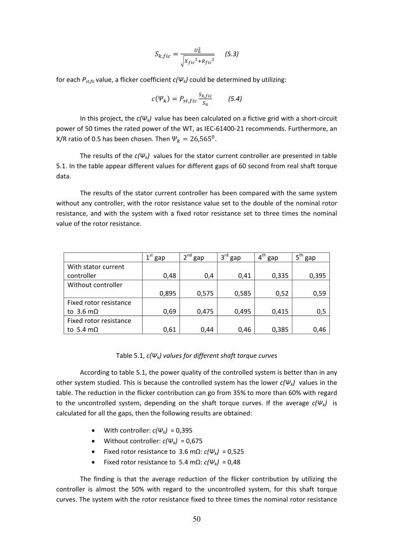
Talking about mechanical stresses, the high–frequency components of the electrical torque are the worst for the machine. So to analyze the mechanical stresses it will be done the FFT (Fast Fourier Transform) of the electrical torque signal. It will give the magnitude of the torque component for each specific frequency. It can be seen in figure 5.15.

Figure 5.15, Periodogram of the electrical torque of the induction machine, in red dashed line without the controller and in dark line with the controller.

What is possible to see in figure above, is that the magnitude of the high‐frequency components of the electrical torque for the system without controller is always higher than the controlled system after f = 1Hz. Then, the curve that represents the non‐controlled system is always above the curve that represents the controlled system. This was expected because by implementing this controller it was pursued to reduce the high frequency components of the torque, which are the worst for the mechanical stresses in the gearbox. These high frequency components have not been eliminated, these have been moved to the low frequencies, were it is possible to see that curve of the controlled system is above the uncontrolled system. This is

10-2 10-1 100 10110-1

100

101

102

Frequency (Hz)

Torq

ue (N

m)

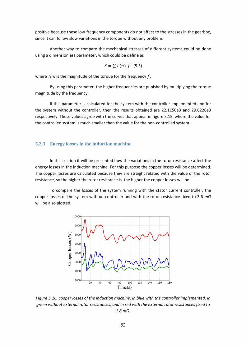
52

positive because these low‐frequency components do not affect to the stresses in the gearbox, since it can follow slow variations in the torque without any problem.

Another way to compare the mechanical stresses of different systems could be done using a dimensionless parameter, which could be define as

∑ (5.5)

where T(n) is the magnitude of the torque for the frequency .

By using this parameter, the higher frequencies are punished by multiplying the torque magnitude by the frequency.

If this parameter is calculated for the system with the controller implemented and for the system without the controller, then the results obtained are 22.1156e3 and 29.6226e3 respectively. These values agree with the curves that appear in figure 5.15, where the value for the controlled system is much smaller than the value for the non‐controlled system.

5.2.3 Energy losses in the induction machine

In this section it will be presented how the variations in the rotor resistance affect the energy losses in the induction machine. For this purpose the copper losses will be determined. The copper losses are calculated because they are straight related with the value of the rotor resistance, so the higher the rotor resistance is, the higher the copper losses will be.

To compare the losses of the system running with the stator current controller, the copper losses of the system without controller and with the rotor resistance fixed to 3.6 mΩ will be also plotted.

Figure 5.16, cooper losses of the induction machine, in blue with the controller implemented, in green without external rotor resistances, and in red with the external rotor resistances fixed to

1.8 mΩ.

20 40 60 80 100 120 140 160 1803000

4000

5000

6000

7000

8000

9000

10000

Time(s)

Coo

per l

osse

s (W

)

53

From figure 5.16, it can be seen that the controlled system has more losses than the system without external rotor resistances, but not much higher, however, much less losses than the system with the rotor resistance fixed to 3.6 mΩ like it could be expected. This is because the average of the rotor resistance selected is 2.4 mΩ, so the copper losses, in average, will be the same as is the rotor resistances of the induction machine were fixed to 2.4 mΩ.

It is true that running a generator at higher slip generates more heat from the generator, which runs less efficiently at has been shown before. But since the increment of these losses is not as much significant as the improvement in the power quality, it is more justified implement this controller. But it always must be present that as higher these losses are, it will be necessary to increase the cooling of the generator.

54

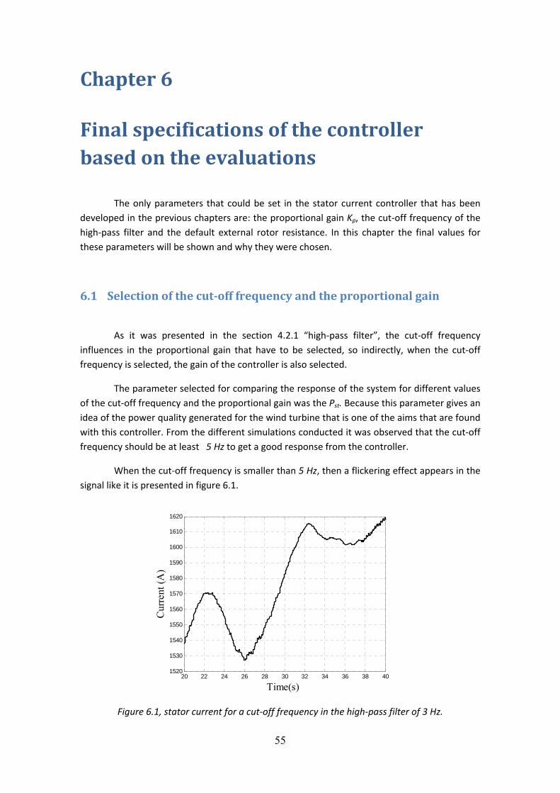
55

Chapter 6

Final specifications of the controller based on the evaluations

The only parameters that could be set in the stator current controller that has been developed in the previous chapters are: the proportional gain Kp, the cut‐off frequency of the high‐pass filter and the default external rotor resistance. In this chapter the final values for these parameters will be shown and why they were chosen.

6.1 Selection of the cut­off frequency and the proportional gain

As it was presented in the section 4.2.1 “high‐pass filter”, the cut‐off frequency influences in the proportional gain that have to be selected, so indirectly, when the cut‐off frequency is selected, the gain of the controller is also selected.

The parameter selected for comparing the response of the system for different values of the cut‐off frequency and the proportional gain was the Pst. Because this parameter gives an idea of the power quality generated for the wind turbine that is one of the aims that are found with this controller. From the different simulations conducted it was observed that the cut‐off frequency should be at least 5 Hz to get a good response from the controller.

When the cut‐off frequency is smaller than 5 Hz, then a flickering effect appears in the signal like it is presented in figure 6.1.

Figure 6.1, stator current for a cut‐off frequency in the high‐pass filter of 3 Hz.

20 22 24 26 28 30 32 34 36 38 401520

1530

1540

1550

1560

1570

1580

1590

1600

1610

1620

Time(s)

Cur

rent

(A)

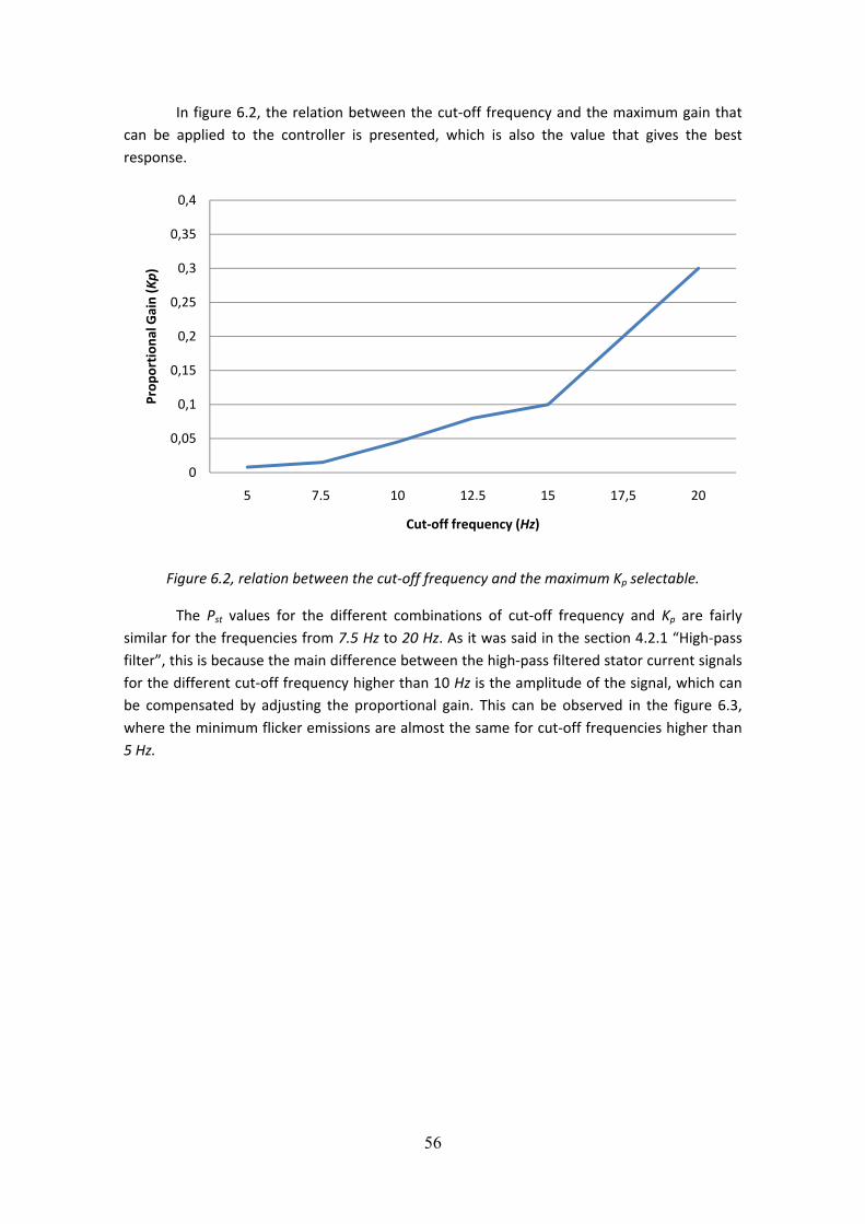
56

In figure 6.2, the relation between the cut‐off frequency and the maximum gain that can be applied to the controller is presented, which is also the value that gives the best response.

Figure 6.2, relation between the cut‐off frequency and the maximum Kp selectable.

The Pst values for the different combinations of cut‐off frequency and Kp are fairly similar for the frequencies from 7.5 Hz to 20 Hz. As it was said in the section 4.2.1 “High‐pass filter”, this is because the main difference between the high‐pass filtered stator current signals for the different cut‐off frequency higher than 10 Hz is the amplitude of the signal, which can be compensated by adjusting the proportional gain. This can be observed in the figure 6.3, where the minimum flicker emissions are almost the same for cut‐off frequencies higher than 5 Hz.

0

0,05

0,1

0,15

0,2

0,25

0,3

0,35

0,4

5 7.5 10 12.5 15 17,5 20

Prop

ortion

al Gain (Kp)

Cut‐off frequency (Hz)

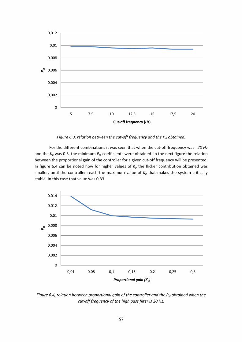
57

Figure 6.3, relation between the cut‐off frequency and the Pst obtained.

For the different combinations it was seen that when the cut‐off frequency was 20 Hz and the Kp was 0.3, the minimum Pst coefficients were obtained. In the next figure the relation between the proportional gain of the controller for a given cut‐off frequency will be presented. In figure 6.4 can be noted how for higher values of Kp the flicker contribution obtained was smaller, until the controller reach the maximum value of Kp that makes the system critically stable. In this case that value was 0.33.

Figure 6.4, relation between proportional gain of the controller and the Pst obtained when the cut‐off frequency of the high pass filter is 20 Hz.

0

0,002

0,004

0,006

0,008

0,01

0,012

5 7.5 10 12.5 15 17,5 20

P st

Cut‐off frequency (Hz)

0

0,002

0,004

0,006

0,008

0,01

0,012

0,014

0,01 0,05 0,1 0,15 0,2 0,25 0,3

P st

Proportional gain (Kp)

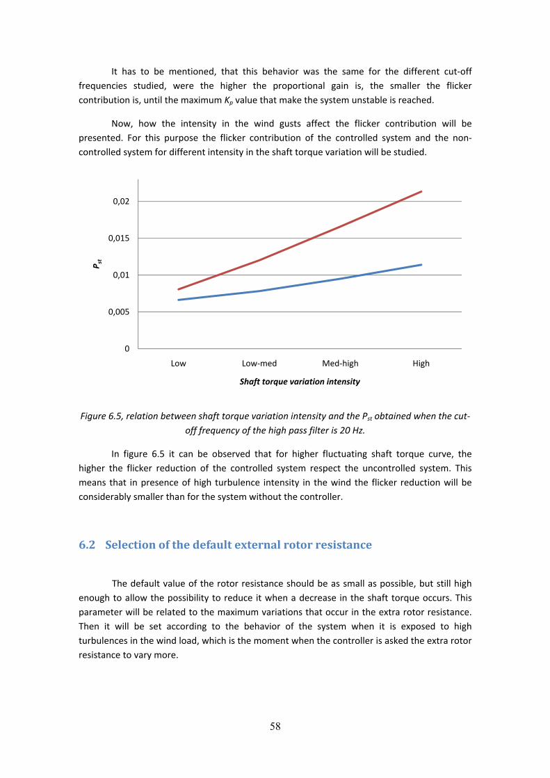
58

It has to be mentioned, that this behavior was the same for the different cut‐off frequencies studied, were the higher the proportional gain is, the smaller the flicker contribution is, until the maximum Kp value that make the system unstable is reached.

Now, how the intensity in the wind gusts affect the flicker contribution will be presented. For this purpose the flicker contribution of the controlled system and the non‐controlled system for different intensity in the shaft torque variation will be studied.

Figure 6.5, relation between shaft torque variation intensity and the Pst obtained when the cut‐off frequency of the high pass filter is 20 Hz.

In figure 6.5 it can be observed that for higher fluctuating shaft torque curve, the higher the flicker reduction of the controlled system respect the uncontrolled system. This means that in presence of high turbulence intensity in the wind the flicker reduction will be considerably smaller than for the system without the controller.

6.2 Selection of the default external rotor resistance

The default value of the rotor resistance should be as small as possible, but still high enough to allow the possibility to reduce it when a decrease in the shaft torque occurs. This parameter will be related to the maximum variations that occur in the extra rotor resistance. Then it will be set according to the behavior of the system when it is exposed to high turbulences in the wind load, which is the moment when the controller is asked the extra rotor resistance to vary more.

0

0,005

0,01

0,015

0,02

Low Low‐med Med‐high High

P st

Shaft torque variation intensity

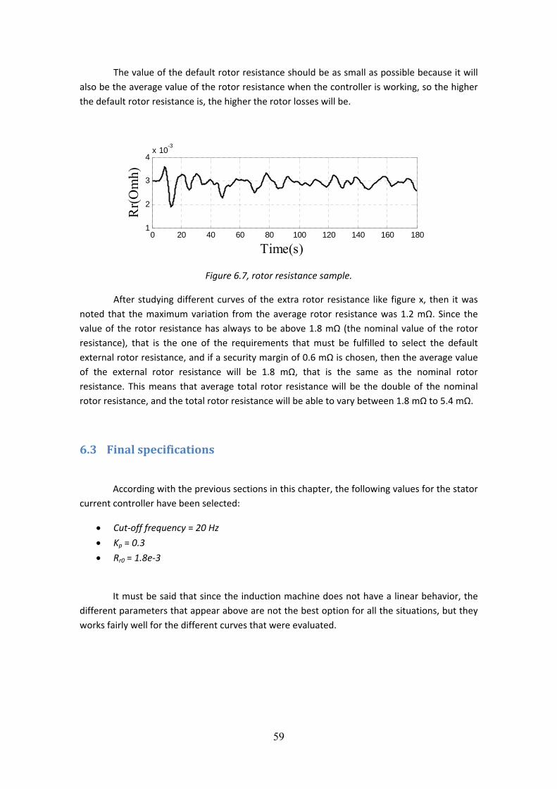
59

The value of the default rotor resistance should be as small as possible because it will also be the average value of the rotor resistance when the controller is working, so the higher the default rotor resistance is, the higher the rotor losses will be.

Figure 6.7, rotor resistance sample.

After studying different curves of the extra rotor resistance like figure x, then it was noted that the maximum variation from the average rotor resistance was 1.2 mΩ. Since the value of the rotor resistance has always to be above 1.8 mΩ (the nominal value of the rotor resistance), that is the one of the requirements that must be fulfilled to select the default external rotor resistance, and if a security margin of 0.6 mΩ is chosen, then the average value of the external rotor resistance will be 1.8 mΩ, that is the same as the nominal rotor resistance. This means that average total rotor resistance will be the double of the nominal rotor resistance, and the total rotor resistance will be able to vary between 1.8 mΩ to 5.4 mΩ.

6.3 Final specifications

According with the previous sections in this chapter, the following values for the stator current controller have been selected:

• Cut‐off frequency = 20 Hz

• Kp = 0.3

• Rr0 = 1.8e‐3

It must be said that since the induction machine does not have a linear behavior, the different parameters that appear above are not the best option for all the situations, but they works fairly well for the different curves that were evaluated.

0 20 40 60 80 100 120 140 160 1801

2

3

4x 10-3

Time(s)

Rr(O

mh)

60

61

Chapter 7

Conclusions

The purpose of this thesis has been to evaluate the behaviour of a wind turbine with an induction generator equipped with a variable rotor resistance. A controller for the variable rotor resistance generator has been developed with the objective of minimizing the torque variations that reduces the mechanical stresses on the shaft of the turbine and also reduces the flicker emission, which leads to a better power quality impact.

In this thesis an induction generator equipped with a variable rotor resistance was analysed and modelled. After that different configurations for the controller were studied to find the best structure for the controller. Finally, the induction machine with the variable rotor resistance controller was compared with the same induction machine without any controller, to study the improvement of implementing the controller.

What was found is that reduction in the flicker contribution by utilising the variable rotor resistance can be between 35%‐60% compared to the uncontrolled system, depending on the shaft torque curves. A higher reduction on the flicker emission was observed for a higher turbulence in the wind.

From this thesis, it can be said that this system generates a smoother electric power in the presence of wind gusts with reduction of the mechanical stress and the mechanical. With a traditional fixed‐speed system, without a variable rotor resistance, in the presence of wind gusts, the power delivered is fluctuating strongly with an increase of the pressures and stress applied to its mechanical elements.

62

63

Chapter 8

Proposed future work

In this thesis an induction machine with a variable rotor resistance has been investigated. As always there are many more interesting aspects that can be taken in consideration. For completion of the model of the wind turbine, a drive train representation should be included in the model. Also a pitch control system should be added to the wind turbine, to ensure that the two control systems co‐operate efficiently, since pitching the blades is a mechanical process, which means that the reaction time for the pitch mechanism will be much higher than for the variable rotor resistance.

Other aspects that could be of interest is to investigate how several of these wind turbines using a variable slip resistance behaves working together. Another interesting issue is the evaluation of a wind farm with these turbines that is connected to the grid over an HVDC line.

64

65

References [1] A. Petersson, T. Thiringer and L. Harnefors, “Flicker reduction of stall‐controlled wind turbines using variable rotor resistances”; Nordic wind power conference, Chalmers University of Technology, 1‐2 March, 2004.

[2] B. Kahinpour ,“Modelling, control and investigation of an HVDC transmission for an offshore wind farm / The centralized control strategy for an offshore wind farm”; Licenciate thesis, Chalmers University of Technology, 2009.

[3] B. C. Kuo and F. Golnaraghi,”Automatic control systems”; John Wiley & Sons, 2003.

[4] CB. Vishwakarma and R. Prasad, “Clustering Method for Reducing Order of Linear System using Pade Approximation”. IETE J Res 2008;54:326‐30.

[5] R. S. Burns, “Advanced control engineering”; Elsevier Ltd, 2001.

[6] J. O. Tande and J. A. Peças Lopes,” Assessment of Power Quality Characteristics of Wind Farms”; IEEE, 2007.

[7] IEC 61400‐21:2001; “Wind turbine generator systems ‐ Part 21: Measurement and assessment of power quality characteristics of grid connected wind turbines”, IEC Standard, 2001.

[8] IEC 61000‐4‐15, “Electromagnetic compatibility (EMC) – Part 4: Testing and measurement techniques – Section 15: Flickermeter ‐ Functional and design specification”, 1997+A1:2003.

[9] T. Thiringer, J. Paixao and M. Bon‐ Giorno, “Monitoring of ride‐through ability of a 2MW Wind turbine in Tvååker, Halland”; Technical Report, Chalmers University of Technology, 2009.

[10] A. Petersson and T. Thiringer, “Control of a Variable‐Speed Pitch‐Regulated Wind Turbine”, Technical Report, Chalmers University of Technology, Göteborg, Sweden, 2005.

[11] T. Thiringer and Andreas Petersson, “Control of a fixed‐pitch variable rotor resistance wind turbine”; Technical Report, Chalmers University of Technology, 2009.

[12] S. Soter and R. Wegener, “Development of Induction Machines in Wind Power Technology”; Institute of Electrical Drives and Mechatronics University of Dortmund, Germany,2003.

[13] G. Franklin J.D. Powell and A. Emami‐Naeini , “Feedback control of dynamic systems”; 5th Edition,Hardcover, 2005.

[14] S. Lundberg, “Wind Farm Configuration and Energy Efficiency Studies ‐ Series DC versus AC Layouts”; Ph.D thesis, Chalmers University of technology, 2006.

[15] ABB Power Technologies AB, “It’s time to connect ‐ Technical description of HVDC Light technology”; Brochure, 2005.

66

[16] T. Burton, D. Sharpe N. Jenkins and E. Bossanyi, “Wind energy handbook”; John Wiley & Sons, Ltd, 2001.

[17] T. Ackermann, R. Leutz, and J. Hobohm, “World‐wide offshore wind potential and european projects,” in Power Engineering Society Summer Meeting, 2001. IEEE, Vancouver, BC, Canada, pp. 4–9 vol.1, 15‐19 June, 2001.

[18] F. lov, F. Blaabjerx and A. D. Hansen, 2. Chen “Comparative Study of Different Implementations for Induction Machine Model in Matlab/Simulink for Wind Turbine Simulations”;IEEE, 2002.