Control of a quadcopter

Pablo Garcıa AunonMaster de Intenierıa de Sistemas y Control

UNED-UCMpablogarciaaunon@gmail.com

June 2015

Abstract

The aim of this master thesis is to analyzed a complex and multivariablesystem, a quadcopter, to model it and develop a controller able to control itsattitude and horizontal and vertical position. The system will be simulated tocheck the system response when implementing this controller.

In the first chapter, a state of the art regarding the controller of the quad-copter is presented. In the second chapter, the dynamic equations of the quad-copter and the model of the motor’s response are developed. The equations arethen simplified by linearizing them around the equilibrium point. In chapter 3,only the rotation equations are considered and a controller presented, whereasin chapter 4 a controller is constructed for the complete model. Since the con-troller are based on a linearlized model, the system response will be checked fora linear and a nonlinear model. In chapter 5 a second controller has been alsopresented, with a more complex control laws, being able to successfully absorbexternal perturbations and changes in the mass of the aircraft. Finally in chap-ter 6, both controllers are compared with different tests and the conclusionspresented.

Chapter 1

Introduction

Quadcopters and their control have being developed in the last 20 years bymany investigation groups all around the world. However, it was only whenthe size, consumption and weight of the computers were reduced, when theseaircraft became popular. Nowadays, their use is being regularized gradually inmany countries and it is expected that they will be used in several civil uses ina near future.

There are presently a wide variety of techniques that may be used to controlthem. In [24] a review of a wide set of different controllers, with their advantagesand their drawbacks, is presented. Normally, the quadcopter’s control is dividedin two different levels; one low level controller, in charge of stabilizing the atti-tude, and a high level one, in charge of controlling the horizontal position. Thevertical movement can be separately controlled.

Linear strategies, and more specifically the well-known PID controllers, mayprovide acceptable results if the movement of the quadcopter is slow and closeto the equilibrium point (hovering). For instance, in [16], the attitude of thequadcopter was stabilized using a PID controller, whereas in [17] the attitudeand the position were controlled by this type of controller. In many cases, theparameters are tuned intuitively by just observing the system response.

PID controllers can be combined with other methods to improve their per-formance. In [22] for example, an helicopter was controlled with a PID, whichis switched to different configurations depending on the aircraft’s state. This isactually an adaptive method, since its configuration changes depending on theenvironment and/or the aircraft state. In that case, an adaptive method wasuse to improve the robustness of the controller, but also if the system presentsnot-well-known characteristics, they might be useful. In [7] for instance, the sys-tem was supposed to have uncertain mass, inertia and aerodynamic dampingcoefficients and the controller was able to deal with these uncertainties.

Another widely used and well-known technique is the backstepping. It con-sists of dividing the system in different levels and stabilizing them one by oneprogressively. In [15], using a quatiernion formulation, a backstepping methodwas implemented to stabilize the attitude of the quadcopter, and Lyapunovfunctions to prove the stability of the system. To improve the robustness of abackstepping controller, in [9] an integrator term was added, eliminating steady-state errors and reducing the response time.

Linear-Quadratic Regulators (LQR) have been also studied. In [2], a PID

1

and a LQR controller are compared. The LQR one, which was based on a morecomplex model, presents better results. Also feedback linearization [19], robustcontrol [3] and intelligent techniques [20][8] are used. Even really demandingcontrollers in terms of computation cost can now be implemented due to theimprove in the micro-computers in the last years, like predictive control tech-niques [5]. Despite here only a couple of techniques have been named, one canget a picture of the diversity of solutions available to control these systems.

In this work, two different backstepping methods are presented and com-pared. These methods converge fast and need less computational efforts, butnormally their robustness is not specially good. Both controllers separate theattitude control from the horizontal and vertical position control. In first place,the attitude is stabilized to lead the quadcopter to the required angles, bycontrolling the traction of the propellers. The horizontal position control is sta-bilized in second place, by assuming that the attitude angles are the variablesthat can be controlled. The first and more simple controller is not able to ab-sorb disturbances, such as horizontal forces or changes in the mass; the secondand more advance one, is capable of handle them. A final comparison will showthese differences.

2

Chapter 2

Dynamics of the quadcopter

In this chapter the dynamics of the quadcopter will be analyzed and a modelto represent the behavior of the system will be proposed. Based on the model,the control’s law will be built up.

2.1 Coordinate frames and transformations

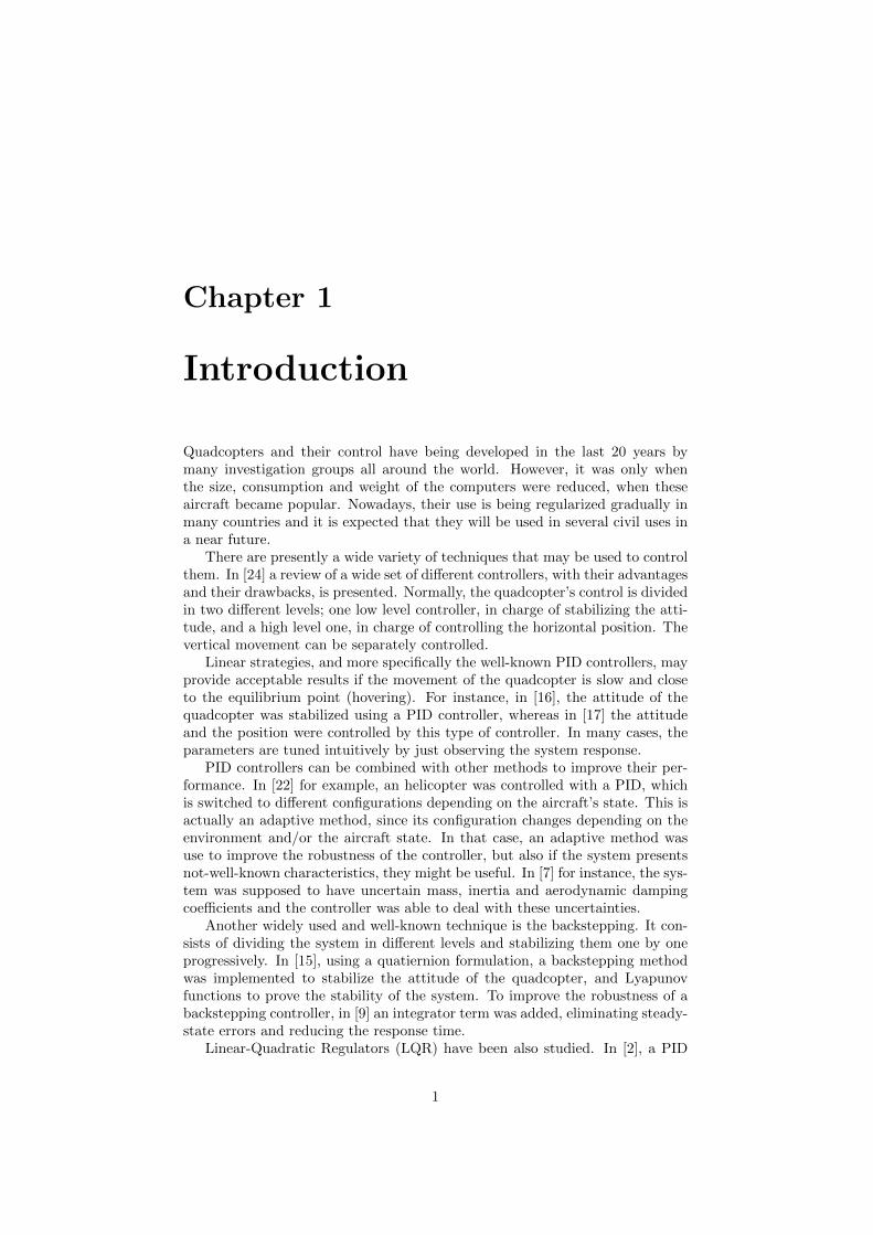
To develop the equations of the quapcopter and its control the next coordinateframes will be used (see Figure (2.1a)):

• Earth frame (intertial frame): fixed to a point in the earth surface, it iscalled ”North-East-Down” system. The zi axes points to the directionof the center of the earth, xi to the North direction and yi to the East.Despite the Earth moves, this frame system can be considered as inertialconsidering the small displacement and low velocity of the quadcopter.

• Vehicle-carried vertical frame: fix to the center of gravity of the quad-copter, its axes are parallel to the Earth frame’s ones.

• Body frame: its origin is located at the center of gravity of the quadcopterand they are fixed to it. Its xbyb plane contains the planes of the rotorsand xbzb is equidistant from all the rotor axes.

To relate the coordinate systems, the Euler angles will be used :

φ: Balance angleθ: Pitch angleψ: Yaw angle

In the Figure (2.1b) those angles have been represented as well as the trans-formation order from Fv (in blue) to Fb (in red). Note that the order of thetransformations is relevant to transform a vector from one system to the other.The transformation matrix is therefore:

Rbv =

cθcψ sφsθcψ−cφsψ cφsθcψ+sφsψcθsψ sφsθsψ+cφcψ cφsθsψ−sφcψ−sθ sφcθ cφcθ

(2.1)

3

(a) Coordinates frame used (b) Euler angles

Figure 2.1: System response with non-zero initial conditions.

This matrix transforms a vector ub referenced in the body frame system Fbto vehicle frame system Fv:

uv = Rvb · ub (2.2)

This transformation matrix might be inverted to make the contrary trans-formation by simply transposing it Rbv = RT

vb.

2.2 Dynamic equations

The quadcopter will be considered as a solid, so that the equations which de-scribe its dynamics are:

dv(t)

dt

∣∣∣∣i

=dvb(t)

dt

∣∣∣∣b

+ ωb × vb = g +Faerom

+Fpropm

(2.3)

dh(t)

dt

∣∣∣∣i

=dhb(t)

dt

∣∣∣∣b

+ ωb × hb =Maero

m+

Mprop

m(2.4)

where

v velocity of the CoG in Fi

vb velocity of the CoG in Fb

h angular moment in Fi

hb angular moment in Fb

ddt

∣∣a

is the derivative in the frame a

ωb is the angular velocity of the quadcopter in Fb

m mass of the quadcopter

g is the acceleration of gravity

4

Faero, Maero aerodynamic forces and moments

Fprop, Mprop the propulsive forces and moments (propellers’ traction)

Every term will be determined in the following subsections.

2.2.1 Aerodynamic forces and moments

In a first approximation, they will be considered as negligible, i.e. Faero ≈Maero ≈ 0. As the quadcopter moves faster, the aerodynamic forces becomehigher and make it to move slower. If fact, if we simulated the movement ofthe quadcopter without having these forces into account, it would accelerateindefinitely, which is clearly unrealistic. Anyway, in this work only slow a dis-placements will be considered and therefore this approximation can be assumed.

2.2.2 Propulsive forces

They are generated by the traction of the 4 propellers installed in the quad-copter. The forces’ direction is always −zb, are always positive and it will beassumed that they do not depend on the relative velocity of the air respect eachpropeller1. Therefore, the transfer function of the traction of each propeller, ui,will be assumed to be:

ui = µωm

s+ ωmvmi (2.5)

where µ is a constant given, ωm is a bandwidth and vmi is the voltagedelivered to the engines. In the Figure (2.2) the traction of each propeller andthe direction of rotation have been represented. The total force, resulting fromadding the traction of each propeller, is then T = u1 + u2 + u3 + u4. Normallya change of variable is used so that the problem is simplified:

u1 + u2 + u3 + u4 = uz (2.6)

2.2.3 Propulsive moments

The moments caused by the traction of the propellers are:

Mx = L = d(u4 − u2) (2.7a)

My = M = d(u1 − u3) (2.7b)

Nz = N = dN (u1 + u3 − u2 − u4) (2.7c)

where d is the distance from the center of the propeller to the CoG in the xbybplane and dN is a fictitious distance which represents the aerodynamic reactionof the propellers due to the draft of the blades. Note that the rotation inertiaof the blades and the motors have been neglected, which will cause moments

1The behavior of the propeller depends highly on it, see [14]. However, such a relativevelocity might be assumed to be much lower than the relative velocity of the air due to thespin of the blades.

5

Figure 2.2: Forces of the propellers and their directions of spin..

around the zb axes. As well as in (2.6), the next change of variables is convenientto be used:

uφ = u4 − u2 (2.8a)

uθ = u1 − u3 (2.8b)

uψ = u1 + u3 − u2 − u4 (2.8c)

On the other hand, the angular moment shall be calculated as:

hb = Ib · ωb (2.9)

where

Ib =

Ix 0 00 Iy 00 0 Iz

ωb =

pqr

Recall that the planes xbyb, xbzb and ybzb are planes of symmetry and there-

fore the non-diagonal elements of the inertia matrix are null.

2.2.4 Equations of the navigation

These equation relate the rotation and the velocity of the quadcopter in thebody frame Fb and its movement in the inertial frame Fi, i.e. the its relativevelocity respect the earth and the Eurler angles:

vv = Rbv · vb (2.11) φ

θ

ψ

=

1 sφtanθ cφtanθ0 cφ −sφ0 sφ/cθ cφ/cθ

ωb (2.12)

6

The Equation (2.11) is simply the transformation of the velocity of the quad-copter in the body frame to the earth frame using Equation (2.1). The Equation(2.12) is calculated taking into account the order in the transformation in theEurler angles.

2.3 Movement equations

Gathering the equations described above one gets finally: u+ wq − vrv + ur − wpw + vp− uq

=

−gsθgcθsφ

gcθcφ− uz/m

(2.13)

Ixp+ (Iz − Iy)rqIy q + (Ix − Iz)prIz r + (Iy − Ix)qp

=

d · uφd · uθdN · uψ

(2.14)

The force equations (2.13) and the moment equations (2.14) together with(2.12) can be integrated to work out the movement of the quadcopter, given thepropulsion of the propellers. Once it is calculated, the displacement in the earthframe can be calculated with (2.11). In the Appendix (A.1) the parameters ofthe quadcopter have been collected. The state of the system will be definedthen:

x =

uvwpqrφθψ

(2.15)

7

2.4 Linearization of the equations

One first approximation to simplify the equations above described is linearizethem around a given point x0. Naming x = x− x0 we get:

˙x =

˙u˙v˙w˙p˙q˙r˙φ˙θ˙ψ

=

−w0q0 + v0r0 − gsθ0−u0r0 + w0p0 + gcθ0sψ0

−v0p0 + u0q0 + gcθ0cψ0

− Iz−IyIxr0q0

− Ix−IzIyr0p0

− Iy−IxIzq0p0

sφ0tθ0q0+cφ0tθ0r0cφ0q0−sφ0r0sφ0q0+cφ0r0

cθ0

+

0 −r0 −q0 0 −w0 −v0 0 −gcθ0 0−r0 0 p0 w0 0 −u0 gcθ0cφ0 −gsψ0sθ0 gcθ0cψ0

q0 −p0 0 v0 u0 0 −gcθ0sφ0 −gsθ0cφ0 0

0 0 0 0 − Iz−IyIxr0 − Iz−IyIx

q0 0 0

0 0 0 − Iy−IxIzr0 0 − Iy−IxIz

p0 0 0 0

0 0 0 − Iy−IxIzq0 − Iy−IxIz

p0 0 0 0 0

0 0 0 1 sφ0tθ0 cφ0tθ0 a1 a2 00 0 0 0 cφ0t sφ0 a3 0 00 0 0 0 sφ0/cθ0 cφ0/cθ0 a4 a5 0

uvwpqr

φ

θ

ψ

+

0 0 0 00 0 0 0− 1m 0 0 0

0 dIx

0 0

0 0 dIy

0

0 0 0 dNIz

0 0 0 00 0 0 00 0 0 00 0 0 0

uzuφuθuψ

(2.16)

having named

a1 = tθ0(cφ0q0 − sφ0r0)

a2 = (1 + t2θ0)(cφ0r0 + sφ0q0)

a3 = −sφ0q0 − cφ0r0

a4 =cφ0q0 − sφ0r0

cθ0

It can be chosen as center point of linealization the quadcopter stabilizedwithout rotation nor displacement (hovering), that is x = 0. Choosing this

8

point, Equation (2.16) becomes:

˙x =

˙u˙v˙w˙p˙q˙r˙φ˙θ˙ψ

=

00g000000

+

0 0 0 0 0 0 0 −g 00 0 0 0 0 0 g 0 00 0 0 0 0 0 0 0 00 0 0 0 0 0 0 0 00 0 0 0 0 0 0 0 00 0 0 0 0 0 0 0 00 0 0 0 0 0 0 0 00 0 0 1 0 0 0 0 00 0 0 0 1 0 0 0 00 0 0 0 0 1 0 0 0

uvwpqr

φ

θ

ψ

+

0 0 0 00 0 0 0− 1m 0 0 0

0 dIx

0 0

0 0 dIy

0

0 0 0 dNIy

0 0 0 00 0 0 00 0 0 00 0 0 0

uzuφuθuψ

(2.18)

Note that now only variables w, p, q and r can be directly controlled, sincethe other terms of the matrix multiplying the control vector are equal to 0.

9

Chapter 3

3dof controller

3.1 Description of the 3dof system

As a first step, before designing a complete controller for the quadcopter, adesign of the 3dof quadcopter is proposed. This system is made up with 4propellers and its structure can rotate around its center of gravity, but its dis-placement is restricted. It will be supposed that the system is equipped bygyroscopes, able to measure the velocity of rotation in every body axes:

y =

pqr

(3.1)

Giving three reference values φr, θr and ψr the system must follow themactuating its 4 motors.

3.2 Simplification of the equations

The Equation (2.18) calculated in the previous chapter considers 6 degrees offreedom. For the system studied in this chapter, that equation shall be simplifiedeliminating the force equations:

˙p˙q˙r˙φ˙θ˙ψ

=

0 0 0 0 0 00 0 0 0 0 00 0 0 0 0 01 0 0 0 0 00 1 0 0 0 00 0 1 0 0 0

pqr

φ

θ

ψ

+

0 dIx

0 0

0 0 dIy

0

0 0 0 dNIz

0 0 0 00 0 0 00 0 0 0

uzuφuθuψ

(3.2)

Note that the control uz has no influence on the state of the system so thatit can be chosen freely.

10

3.3 Design of the linear controller

Since the linealized equations are decoupled, each controller can be design sep-arately. Taking as example the control of φ, from Equation (3.2) one has:

˙p = dIxuφ

˙φ = p

}→ ¨φ =

d

Ixuφ (3.3)

To control the variable φ, a PID controller is be proposed. With the Laplacetransform of the previous equation we get:

s2Ixd

Φ(s) = Uφ(s) (3.4)

If we suppose now that when Uφ is commanded, the commands for theengines 4 and 2 are equal and but with different sign, Uφ = U4 − U2 = 2U4,from Equations (2.5) and (2.8) we obtain:

s2Ixd

Φ = Uφ = 2 · U4 =2µωms+ ωm

Vm4=

2µωms+ ωm

Vφ (3.5)

and therefore the forward-path transfer function is:

Φ

Vφ= Gp(s) =

2µωmd

Ix

1

s2(s+ ωm)= kφ

1

s2(s+ ωm)(3.6)

The PID controller has the following transfer function Gc(s):

Gc = kP +kIs

+ kD · s (3.7)

Having a unity feedback gain, the transfer function of the close-loop systemturns out to be:

Hφ(s) =Gc ·Gp

1 +Gc ·Gp= kφ

kDs2 + kP s+ kI

s4 + s3ωm + kφ(kDs2 + kP s+ kI)(3.8)

In a similar way, we can get the transfer function of the system for the ψangle:

Hψ(s) = kψkDs

2 + kP s+ kIs4 + s3ωm + kψ(kDs2 + kP s+ kI)

(3.9a)

kψ =4µωmdN

Iz(3.9b)

Having a look at the previous equations, we can realize that analyticallywould not be easy to choose the coefficient of the PID controller, even simplifyingthe equation considering kI � 1. Therefore, the parameters will be determinedwith the help of the PID Tune toolbox within Simulink to reach a suitablebehavior; although this tool does not represent exactly the behavior of thecomplete system, it helps as a first step to select the parameters of the controller.Since there have not been specified any performance requirement, it will be triedthat the system response is as fast as possible with an overshoot lower than 5%,

11

Parameter PID - φ, θ PID - ψ

kP 0.0055 1kI 0.0007 0kD 0.9 4.9N 35 100

BM (rad/s) 5.37 2.74Mr 1.03 1.09

ωr (rad/s) 1.57 0.47

Table 3.1: Values of the parameters of the 3 dof PID controller and their maincharacteristics extracted from the Bode diagram.

taking into account the saturation of the motors. For the angle ψ, since thevelocity response is not critical, the overshooting will be set to zero, and thesystem response will not be required to be as fast as possible, ensuring thenthat the effort needed from the motors is lower.

In the Table (3.1) the parameters of the controller have been written. Noticethat there is a parameter, N , which normally is not used. It is the FilterCoefficient, which is the pole of the derivative term (an ideal derivative termwould have N =∞). The transfer function of the controller is then:

FPID(s) = kP +kIs

+ kDN · ss+N

(3.10)

This coefficient fillers the signal before deriving it, so that higher frequenciesthan N are absorbed. The higher N is, the wider the considered bandwidth ofthe signal is.

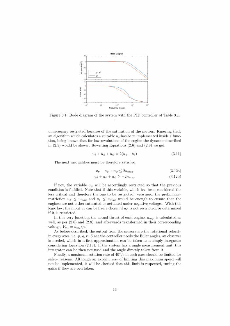
The some aspects of the performance of the system might be obtained withthe frequency-domain analysis, as well a some conclusions about the sensitivityand robustness of it. In Figure 3.1 the Bode diagram of the system response, seeEquations 3.8 and 3.9, with the PID controller of Table 3.1 has been represented.From it, the Bandwidth (BM), the Resonant Peak (Mr) and the Resonant Fre-quency (ωr) can be obtained; in Table 3.1 all these values have been presented.Note that the bandwidth of the yaw control is lower than the pitch one, whichmeans that for reference signals whose frequencies are higher than this value,the system will have difficulties to follow them. This result is actually consis-tent, since the dynamics of the system is slower rotating around the zb axes.Anyway, as it was already pointed out, the yaw requirements are not expectedto be very demanding and therefore this result is acceptable.

Once the inputs uφ, uθ and uψ have been calculated, they must be trans-formed to the inputs of each motor. Notice that there is a variable not yetdetermined, uz, since the movement in the zb direction is impeded. Therefore,to determine the 4 inputs, this last variable must be chosen. If it were simplytaken as 0, when one the other variables were determined, it would lead to anegative thrust in at least one engine. The easiest solution might be simply as-sign a positive value to uz, e.g. the weight, high enough to avoid that situation;this would be the trimming of the system if it were a quadcopter able to movein the vertical direction, which is not the case. In the case here studied, a 3dofquadcotper, this choice would not be the optimal, since the output could be

12

Mag

nitu

de (

dB)

-60

-40

-20

0

20

φ, θψ

10-2 10-1 100 101 102

Pha

se (

deg)

-180

-135

-90

-45

0

45

Bode Diagram

Frequency (rad/s)

Figure 3.1: Bode diagram of the system with the PID controller of Table 3.1..

unnecessary restricted because of the saturation of the motors. Knowing that,an algorithm which calculates a suitable uz has been implemented inside a func-tion, being known that for low revolutions of the engine the dynamic describedin (2.5) would be slower. Rewriting Equations (2.6) and (2.8) we get:

uθ + uφ + uψ = 2(u4 − u3) (3.11)

The next inequalities must be therefore satisfied:

uθ + uφ + uψ ≤ 2umax (3.12a)

uθ + uφ + uψ ≥ −2umax (3.12b)

If not, the variable uψ will be accordingly restricted so that the previouscondition is fulfilled. Note that if this variable, which has been considered theless critical and therefore the one to be restricted, were zero, the preliminaryrestriction uφ ≤ umax and uθ ≤ umax would be enough to ensure that theengines are not either saturated or actuated under negative voltages. With thislogic law, the input uz can be freely chosen if uψ is not restricted, or determinedif it is restricted.

In this very function, the actual thrust of each engine, umi , is calculated aswell, as per (2.6) and (2.8), and afterwards transformed in their correspondingvoltage, Vmi = umi/µ.

As before described, the output from the sensors are the rotational velocityin every axes, i.e. p, q, r. Since the controller needs the Euler angles, an observeris needed, which in a first approximation can be taken as a simply integratorconsidering Equation (2.18). If the system has a angle measurement unit, thisintegrator can be then not used and the angle directly taken from it.

Finally, a maximum rotation rate of 40◦/s in each axes should be limited forsafety reasons. Although an explicit way of limiting this maximum speed willnot be implemented, it will be checked that this limit is respected, tuning thegains if they are overtaken.

13

time (s)0 5 10 15 20

angl

e (d

eg)

-5

0

5

10

15

20

φ

θ

ψ

(a) Euler angles

time (s)0 0.5 1 1.5 2

Vm

(V

)

-5

0

5

10

15

20

25

V1

V2

V3

V4

(b) Inputs

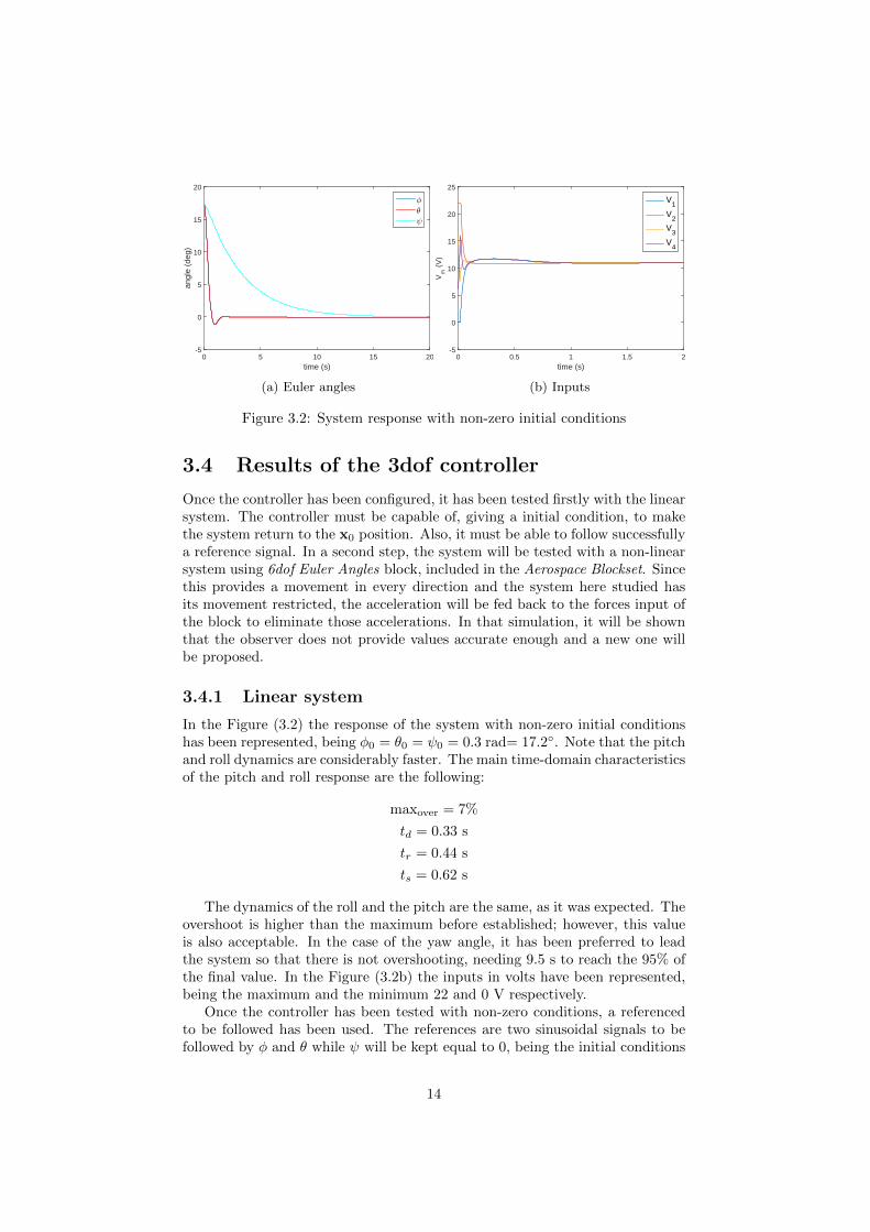
Figure 3.2: System response with non-zero initial conditions

3.4 Results of the 3dof controller

Once the controller has been configured, it has been tested firstly with the linearsystem. The controller must be capable of, giving a initial condition, to makethe system return to the x0 position. Also, it must be able to follow successfullya reference signal. In a second step, the system will be tested with a non-linearsystem using 6dof Euler Angles block, included in the Aerospace Blockset. Sincethis provides a movement in every direction and the system here studied hasits movement restricted, the acceleration will be fed back to the forces input ofthe block to eliminate those accelerations. In that simulation, it will be shownthat the observer does not provide values accurate enough and a new one willbe proposed.

3.4.1 Linear system

In the Figure (3.2) the response of the system with non-zero initial conditionshas been represented, being φ0 = θ0 = ψ0 = 0.3 rad= 17.2◦. Note that the pitchand roll dynamics are considerably faster. The main time-domain characteristicsof the pitch and roll response are the following:

maxover = 7%

td = 0.33 s

tr = 0.44 s

ts = 0.62 s

The dynamics of the roll and the pitch are the same, as it was expected. Theovershoot is higher than the maximum before established; however, this valueis also acceptable. In the case of the yaw angle, it has been preferred to leadthe system so that there is not overshooting, needing 9.5 s to reach the 95% ofthe final value. In the Figure (3.2b) the inputs in volts have been represented,being the maximum and the minimum 22 and 0 V respectively.

Once the controller has been tested with non-zero conditions, a referencedto be followed has been used. The references are two sinusoidal signals to befollowed by φ and θ while ψ will be kept equal to 0, being the initial conditions

14

time (s)0 5 10 15 20

angl

e (d

eg)

-15

-10

-5

0

5

10

15

φ

θ

ψ

(a) ωφ = ωθ = 0.5 rad/s

time (s)0 0.2 0.4 0.6 0.8 1

angl

e (d

eg)

-15

-10

-5

0

5

10

15

φ

θ

ψ

(b) ωφ = ωθ = 10 rad/s

Figure 3.3: System response with zero initial conditions and sinusoidal referencesignal with an amplitude of 0.2 rad, 11.5◦.

equal to zero. In the Figure (3.3) the input of the system has been representedas well as the reference signals (dashed lines) for two different frequencies, 0.5and 10 rad/s. For the lower frequency, see Figure 3.3a, the attenuation is barelyvisible, around +0.035 dB, and a phase delay of 8.9◦, 0.31 s. From the Bodediagram we would have expected an attenuation of +0.025 dB and a phase delayof 7.5◦, which matches pretty well. This results shows that the controller is ableto follow successfully the reference signal. If the frequency increases up to 10rad/s, the situation is completely different, as can be seen in Figure 3.3b. Theattenuation is clearly visible as well as the phase delay. From the graphic weidentify an attenuation of -13.8 dB and a phase delay of 158◦, whereas withthe Bode diagram we would expect -11.9 dB and 135◦. Note also that the firstcycles of the system response do not represent the steady state and thereforethe attenuation and the phase delay have been identified after some oscillations.

The results obtained directly from the system response are not exactly thesame as the ones obtained from the Bode diagram, although both are similar.The differences might be due the derivative block of the PID controller, in whichthe coefficient N is not infinity, what has been assumed in Equation 3.7.

3.4.2 Non-linear system

The controller has been designed assuming the system as linear. Although forsmall angles it is a good approximation, if it is not the case, the result may bereally different. On the other hand, the rotation in every axes is coupled, as canbe seen in (2.14), so that when the rotations in the different axes are managedat the same time, the behavior is non-linear.

In the Figure (3.4a) the response of the non-linear system has been shown,with the same controller and observer previously used. It must be said, that theangles here shown are the estimated by the linear observer, which it is nothingbut an integration of the linear Equations (3.2) to obtain the euler angles. Theresult seems to be pretty the same as the one obtained using the linearizedsystem, Figure (3.3b). However, if one observes the real angles, assumed to bethe ones calculated by the 6dof Euler Angles block, one realizes that the yawangle is not kept in 0◦as requested, but oscillates periodically with an amplitude

15

time (s)0 5 10 15 20

angl

e (d

eg)

-15

-10

-5

0

5

10

15

φ

θ

ψ

(a) Measurements from the linear observer

time (s)0 5 10 15 20

angl

e (d

eg)

-15

-10

-5

0

5

10

15

φ

θ

ψ

(b) Real values

Figure 3.4: Non-linear system response with zero initial conditions and sinu-soidal reference signals with ωφ = ωθ = 0.2 rad/s

time (s)0 5 10 15 20 25 30 35 40

angl

e (d

eg)

-15

-10

-5

0

5

10

15

φ

θ

ψ

Figure 3.5: Non-linear system response with zero initial conditions and sinu-soidal reference signals with ωφ = ωθ = 0.2 rad/s and non-linear observer

.

1.2◦and a mean value of -0.6◦. This is due to the fact that a linear observerhas been used to calculate a movement which is not linear in reality. Beside theoscillation of ψ, apparently, there is no change in the response of the system,which means that with this frequency the system still behaves as linear.

To improve the yaw response, an improved observer has been used afterwardswhich integrates (2.12) to calculate a more accurate value of the attitude of thequadcopter. In the Figure (3.5) the response of the non-linear system, using thenew non-linear observer has been represented. The system keeps on oscillating inthe yaw axes but now the mean value has been moved to 0◦and the amplitudereduced to only 0.2◦, being this result considerably better. The oscillationaround 0◦still exists because the controller is not fast enough to cancel it.

16

Chapter 4

6dof linear controller

4.1 Description of system

Once the controller for the 3dof quadcopter has been developed, a new con-troller for the complete 6dof quadcopter is wanted, using the first stabilizationcontroller for the attitude, angles φ, θ and ψ. The design firstly must be ex-tended to control the movement in the zb direction so that the quadcopter iscapable of being stabilized in both horizontal axes and in the vertical directionindependently. Finally, a higher level controller will be implemented in order toallow the quadcopter to move from one point to another, being the coordinatesof those points given in the inertial coordinate frame.

The physical properties of the quadcopter are presented in the Appendix(A.2). The behavior of the quadcopter will be probably more agile, since Ix, Iy,Iz and m decrease, and the product µ · Vmax increases. On the other hand, ωmincreases as well, which means that the dynamic of the engines is faster thanthe one of the 3dof quadcopter.

4.2 Architecture of the controller

In the Figure (4.1) the architecture of the 6dof controller has been representedwith its different components. First, we have the Quadcopter, which representsthe quadcopter itself and provides the measurements of the gyroscopes and ac-celerometer to the Observer. This, using that information, processes it andcalculates the state of the quadcopter, i.e. global position and attitude, deliv-ering it to both controller levels. The High Level Controller, having as inputthe estimated position and the Desired position and orientation, calculates theneeded attitude angles and the altitude in the zi direction (which is approxi-mately zb) to reach the destination point. Finally, the Lower Level Controllerprovides the required voltages (Vm) to the engines of the quadcopter so that thevales φ, θ, ψ and zd are reached adequately. Every component of the systemwill be described in detail.

17

Quadcopter

Observer

High Level Controller

Low Level Controller

𝑦

𝑥

𝜙𝑑, 𝜃𝑑, 𝜓𝑑, 𝑧𝑑 𝑉𝑚

𝑥

Desired positionand orientation

𝑋, 𝑌, 𝑍, 𝜓𝑑

Figure 4.1: Architecture of the 6dof controller.

4.2.1 Quadcopter

The model used to represent the quadcopter is, as used for the design of the3dof controller, the 6dof Euler Angles block integrated in Simulink, but now thedisplacement will be allowed and the weight will be included as external forcein the direction of zi. The model of the dynamic of the engines, Equation (2.5),will be also included. The output will be the acceleration and the velocity ofrotation in every axes of the body frame Fb.

4.2.2 Observer

The observer here developed is an extension of the non-linear observer used inthe 3dof controller. Given the velocity of rotation in every body axex, wb, it isintegrated using Equation (2.12) and the attitude is then calculated. With it,the acceleration vector can be transformed from the body frame to the inertialframe using the matrix of the Equation (2.1), and finally integrated twice tocalculate the global position.

Notice that this observer has two important problems. First, the attitudeangles are an integration of the velocity of rotation, which means that alongthe time, errors are integrated as well and this leads to an increase, linearlydependent on time, of the errors in the measurements of those angles. In thecase of the the global position, it is calculated by integrating the accelerationtwice, so the errors may become bigger even faster. Despite this fact, the firstproblem is more critical, since it affects directly to the safety of the aircraft.

Finally, as it will be said afterwards, the High Level Controller needs anestimation of the total thrust of the propellers, i.e. uz, which will be providedby the observer as well knowing the voltage provided to the motors, Vmi .

18

Parameter PID - φ, θ PID - ψ PID - z

KP 0.0015 1 5KI 0 0 0KD 0.4 2.2 5N 50 150 50

BM (rad/s) 7.33 9.18 -Mr 1.00 1.07 -

ωr (rad/s) 0.004 1.40 -

Table 4.1: Values of the parameters of the 6dof PID controller

4.2.3 Low Level Controller

The Low Level Controller is in charge of stabilizing the attitude of the quad-copter given the desired Euler angles, and of controlling the movement in thedirection zb. The same structure will be used as for the 3dof quadcopter, butthe function which used to control the saturation of the motors will no be usedanymore, since the the variable uz is also given, and the voltage output to themotors will be restricted to its limits. On the other hand, since the parametersof the quadcopter have changed, see Appendix (A.2), the PID controllers mustbe tuned again to get a good response of the system.

In the Table (4.1) the parameters of the 6dof controller has been shown, withthe new PID controller for the zb direction. The coefficients are now lower, sincethe dynamic of the quadcopter is faster (lower mass and inertia and higher thrustof the motors), while the pole of the derivative term, N , has been increased.

Equations (3.8) and (3.9) are still valid for this controller, but with theparameters updated. Following a similar procedure, one can obtain the equationin the Laplace plane that describes the movement in the z axes:

Z(s) = kz(kDs

2 + kP s+ kI)Zr(s) +g

ss4 + s3ωm + kz(kDs2 + kP s+ kI)

(4.1a)

kz =4µωmm

(4.1b)

Since it is not possible to explicitly separate the transfer function, the bodediagram cannot be directly drawn. Instead of it, the robustness of the controllerwill be tested in Section 6.2 by applying a vertical force on the quadcopter andchanging its mass.

In Figure 4.2 the Bode diagram of the θ/φ and ψ controllers has been rep-resented. As they have been designed, the frequency response is very similar.Also, in Table 4.1 the bandwidth, the peak and the peak frequency have beenpresented. Note that the bandwidth is now higher, meaning that the systemresponse is faster than the 3dof one.

The configuration of the PID controllers has been tested for changes in theyaw and pitch angles up to 0.3 rad, 17◦, keeping in mind that the maximumspin rate in every axes is 40◦/s. In the Figure (4.3) the response of the systemhas been represented, with step reference signals of 1 m for z, 0.3 rad (17.2◦) forthe pitch and roll angles and 1 rad (57.3◦) for the yaw angle. z is the altitude in

19

Mag

nitu

de (

dB)

-80

-60

-40

-20

0

20

φ, θψ

10-1 100 101 102 103

Pha

se (

deg)

-180

-135

-90

-45

0

Bode Diagram

Frequency (rad/s)

Figure 4.2: Bode diagram of the system with the PID controller of Table 4.1..

Characteristic PID - φ, θ PID - ψ PID - z

maxover (%) 0 0.4 0td(s) 0.31 1.49 0.41tr 0.63 2.34 1.00ts 0.90 4.53 1.55

Table 4.2: Time characteristics of the three controllers, obtained from the resultsof Figure 4.3.

the inertial coordinate frame, Fi, since the observer transforms the accelerationsfrom the body frame to that one. Note that when the aircraft tilts, it loosesaltitude slightly because the controller does not compensate directly the lack ofthrust in the zi component, but only when the PID controller acts due to thedifference between the altitude and the reference signal.

In Table 4.2 the time characteristics of the three controllers have been pre-sented, as well as the overshooting. Opposed to the 3dof controller, these havebeen designed so that they do not have overshooting; also, we can remark thatthe response is now faster, as it was expected.

4.2.4 High Level Controller

This level of the controller is in charge of generating the reference signals forthe attitude and the altitude to be followed by the Low Level Controller, sothat being given a destination point in the inertial coordinate frame and anorientation, the quadcopter reaches it.

To control the variables ui and vi, which are the velocities in the inertialframe and are not directly controllable, the backstepping method will be used.This technique basically assumes as controllable a variable which is not actually,and once its wanted value is known, the system is controlled to reach that value.Assuming values of the attitude small, i.e. φ, θ, ψ � 1, the system can be

20

z [m

]

-1

-0.5

0

φ [°

]

0

10

20

θ [°

]

0

10

20

time [s]0 5 10 15 20 25 30 35 40

ψ [°

]

0

20

40

60

Figure 4.3: Response of the system with step reference signals..

21

linearized and from Equation (2.13) one gets:

ub = −gθ (4.2a)

vb = gθ (4.2b)

wb = g − T/m (4.2c)

Knowing also that ub = Rbvuv, finally we have that:

ui = −θ Tm

(4.3a)

vi = φT

m(4.3b)

Then to control ui and vi we will assume as controllable the variables θ andφ, being T an estimation of total thrust of the propellers, commanded by thealtitude control. If those variables are chosen as:

θd = −mT

(Xd + kDx(Xd − X) + kPx(Xd −X)

)(4.4a)

φd =m

T

(Yd + kDy (Yd − Y ) + kPy (Yd − Y )

)(4.4b)

where X and Y are the position in the inertial frame and Xd and Yd are thedesired position in that very frame, Equations (4.3) become:

ex + kDx ex + kPxex = 0 (4.5a)

ey + kDy ey + kPyey = 0 (4.5b)

having called ex = Xd−X and ey = Yd−Y . The constants kDx , kPx , kDy andkPy must be chosen properly so that the system converge to ex = ey = 0. Forthis case, having tested the complete system, the values taken are:

kDx = kDy = 2.2

kPx = kPy = 1

Once the wanted values, θd and φd, are known, the Low Lever Controlleracts to drive the system to them. The values of zd and ψd are simply passed toit.

It has been assumed that the attitude angles are small and therefore thesystem can be linearized, getting Equation (4.3). However, the yaw angle mightnot be negligible at all. To solve this assumption, a change of the coordinatesof the destination points must be carried out:[

X

Y

]=

[cosψ − sinψsinψ cosψ

] [XY

](4.7)

Given a position in the inertial frame, X and Y , the controller first changethe coordinate system so that ψ = 0, getting X and Y . Afterwards, it calcu-lates θd and φd through the Equations (4.4), delivering them to the Low LevelController.

22

time [s]0 20 40 60 80 100 120

-1

-0.5

0

0.5

1 XYZ

(a) Position of the quadcopter in inertialframe coordinates

Y [m]

1

0.5

010.80.6

X [m]

0.40.20-0.2

1.2

0

0.2

0.4

0.6

0.8

1

-Z [m

]

(b) Trajectory of the quadcopter

Figure 4.4: Test of the 6dof controller, following a predefined trajectory

4.3 Results of the 6dof controller

In order to test that the controller works properly, the quadcopter will be com-manded to reach some points in the space with a specific orientation. Firstly, thequadcopter will ascend to zi = −0.5 m and then trace a 1-meter-side square inthe space with an orientation of ψd = 0. Having completed that, it will changeits orientation to ψd = π/4 and repeat the same movement in the space butwith an altitude of zi = −1. Despite the orientation changes, the quadcoptermust be capable of reaching the points anyway.

The movement of the quadcopter has been represented in Figure 4.4, follow-ing the trajectory above described. In the Figure 4.4a the position in inertialframe coordinates are shown; once the quadcopter reaches zi = −0.5 m, itmoves forward and then to the left, coming back to the origin. Afterwards,it changes again its high to zi = −1 m and its orientation to ψd = π/4 andrepeats the same movement. Note that even with the change in the orientationthe quadcopter reaches the destination points successfully. In the Figure 4.4bthe 3d movement, estimated by the Observer, has been represented, indicatingthe orientation with the blue arrows at some points of the trajectory.

Considering a step input of 1 m, see Figure 4.4a, the time characteristics ofthe system response in the x and y direction are:

maxover = 0

td = 1.58 s

tr = 3.72 s

ts = 5.51 s

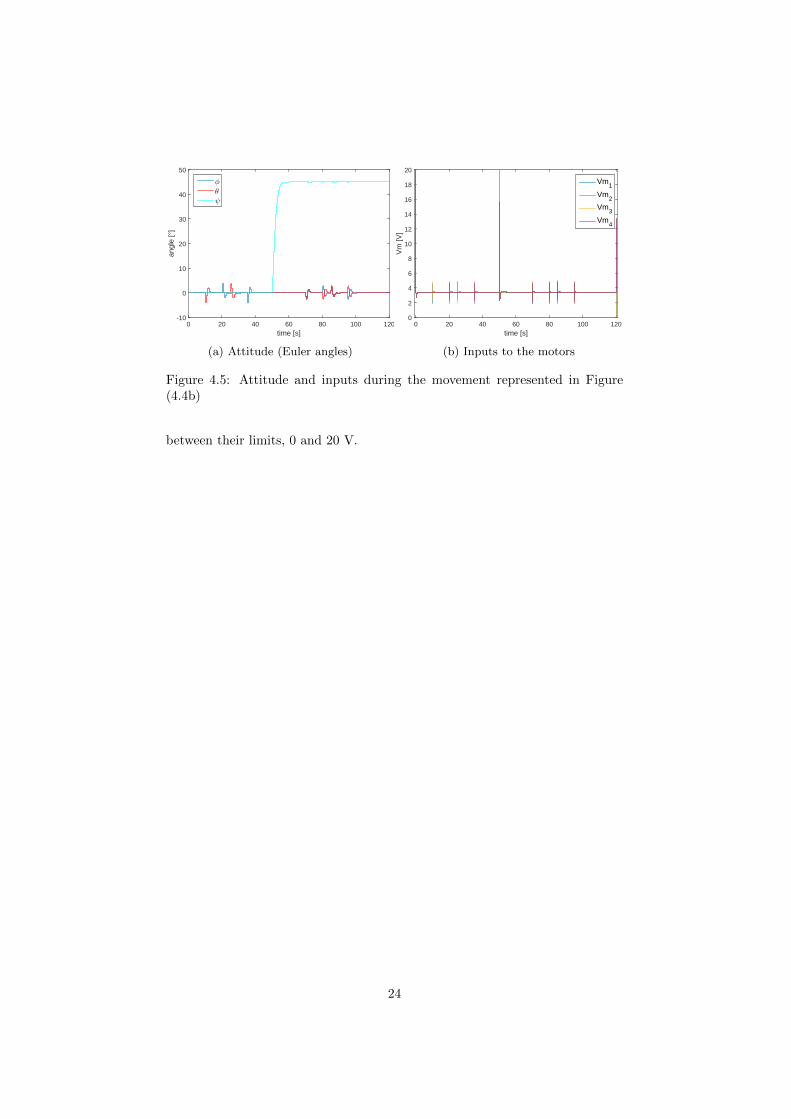
The attitude and the input of the motors haven represented in Figure 4.5aand 4.5b respectively. The change in the pitch and roll angles needed to reachthe velocities in every direction are actually small (∼5◦) so that the linealizedsystem is closed to the real one. On the other hand, once the yaw angle changes,the distribution of pitch and roll angles change as well to achieve the attitudeto reach the destination points in the second level of the travel (in the planezi = −1). As it can be seen in the Figure (4.5b) the inputs remains always

23

time [s]0 20 40 60 80 100 120

angl

e [°

]

-10

0

10

20

30

40

50

φ

θ

ψ

(a) Attitude (Euler angles)

time [s]0 20 40 60 80 100 120

Vm

[V]

0

2

4

6

8

10

12

14

16

18

20

Vm1

Vm2

Vm3

Vm4

(b) Inputs to the motors

Figure 4.5: Attitude and inputs during the movement represented in Figure(4.4b)

between their limits, 0 and 20 V.

24

Chapter 5

Advanced backsteppingcontroller

A new a more advanced controller will be presented, which is based on thebackstepping technique, but is build up with more complex laws, capable ofabsorbing external forces and changes in the mass. This controller is presentedin [9] and the main contribution of this work is how the parameters have beenselected by using a genetic algorithm.

First, we define a new frame coordinate system k, whose center is the centerof gravity of the quadcopter, its x axes correspond to the k2 axes (see Figure2.1b), y axes is k1 and z is zv. The angular velocity of this new system isthe ωk = [0, 0,−ψ] so that it can be neglected in Equation (2.3), since it canbe expected only low values of yaw velocities. Taking the state of the systemof Equation (2.15) represented in the frame k, the equation of the motion isx = f(X,U), being

f(X,U) =

uz·Ux+Dxm

uz·Uy+Dym

−uz·cosφ cos θm + Dz

m + g

Iy−IzIx

rq + dIx· uφ

Iz−IxIy

pr + dIy· uθ

Ix−IyIz

qp+ dNIz· uψ

p

q

r

(5.1)

where Di are disturbances, in N, in every axes; ux and uy are the coefficientsto project the traction in both axes:

−ux = cosφ sin θ cosψ + sinφ sinψ (5.2a)

−uy = cosφ sin θ sinψ − sinφ cosψ (5.2b)

25

Three different controllers will be developed: attitude, position and altitude,based on the backstepping technique. In the three cases, we have a system oftwo variables:

x1 = x2 (5.3a)

x2 = a · u+ b (5.3b)

where u is the controllable variable which, as it can be seen, cannot directlycontrol x1, the variable to be controlled. We define then the error for thevariable to be controlled and for the pseudo control variable x2:

e1 = x1d − x1 (5.4a)

e2 = x2d − x2 (5.4b)

being x1d the desired value of the variable to be controlled. Note that x2d canbe chosen freely. A Lyapunov function is proposed:

V =1

2λp2 +

1

2e21 +

1

2e22 (5.5)

having defined p = e1. To ensure the convergence of the system, the functionV must be positive-definite and its derivative negative-definite:

V = λpp+ e1e1 + e2e2 (5.6)

knowing that e1 = x1d − x1 = x1d + e2 − x2d, we finally get:

V = λpe1 + e1(x1d − x2d) + e2(e2 + e1) (5.7)

choosing

x2d = x1d + c1e1 + λp (5.8a)

e2 = −e1 − c2e2 (5.8b)

the derivative of the Lyapunov function turns out to be:

V = −c1e21 − c2e22 (5.9)

which is definite-negative and ensures the convergence. Deriving Equations(5.8a) and (5.8b) and with Equation (5.3b), we finally get the control law:

u =(1− c21 + λ)e1 + (c1 + c2)e2 − c1λp+ x1d − b

a(5.10)

The integer term of the controller will be implemented as adaptive, so thatwhen the error is lower than a certain limit, p is non zero:

p =

{0 if e1 ≥ e1λlimp if e1 < eλlim

(5.11)

This will reduce the overshooting of the system.

26

5.1 Attitude control

To control the three attitude variables θ, φ and ψ, Equation (5.10) shall be used,being from Equation (5.1):

bφ =Iy − IzIx

rq aφ =d

Ix(5.12a)

bθ =Iz − IxIy

pr aθ =d

Iy(5.12b)

bψ =Ix − IyIz

qp aθ =dNIz

(5.12c)

5.2 Position control

The position controller differs from the one developed for the attitude controlbecause of the consideration of a perturbation force Di in both axes. However,a similar procedure will be followed. These perturbations will be estimated andincluded in the control law:

Di = Di − Di (5.13)

where Di is the estimated value of the perturbation, D is the actual perturbationvalue and Di is the error made. These perturbations will be considered asconstant, or better said, its dynamics are much slower than the ones involvedin the estimation of the perturbation:

˙Di ' − ˙Di (5.14)

Having said that, let’s assume that there exists, for the control along the xaxes, the next Lyapunov function:

V = V (px, e1x, e2x, D) (5.15)

whose derivative would be:

V = px∂V

∂px+ e1x

∂V

∂e1x+ e2x

∂V

∂e2x+ ˙Dx

∂V

∂Dx

(5.16)

Considering Equations (5.3a), (5.4b), (5.8a) and (5.4b), the error ex2 can becalculated as:

e2x = c1xe1x + x1d + λxpx − x1 (5.17)

and with Equation (5.14) we get:

V = px

(∂V

∂px+ λx

∂V

∂e2x

)+ e1x

(∂V

∂e1x+ c1x

∂V

∂e2x

)+

+

(xd −

uxu1 +Dx

m

)∂V

∂e2x− ˙Dx

∂V

∂Dx

(5.18)

ux shall be chosen so that the function V is definite negative. Making u1

m ux =

ux1 + ux2 and ux1 = xd − Dx, the previous equation is simplified to:

V = px

(∂V

∂px+ λx

∂V

∂ex2

)+ ex1

(∂V

∂ex1+ cx1

∂V

∂ex2

)− ux2

∂V

∂ex2

−Dx −Dx

m

∂V

∂ex2− ˙Dx

∂V

∂Dx

(5.19)

27

Now, lets divide again the term ux2 into two, ux2 = ux3 + ux4, and takingux3 = pxλx + e1xc1x, we get:

V = px∂V

∂px+ e1x

∂V

∂e1x− ux4

∂V

∂e2x− Dx

m

∂V

∂e2x− ˙Dx

∂V

∂Dx

(5.20)

The last term can be chosen as:

ux4 =px

∂V∂px

+ e1x∂V∂e1x

∂V∂e2x

+ kx∂V

∂e2x

and as result, the derivative is:

V = −kx(∂V

∂ex2

)2

− Dx

m

∂V

∂ex2− ˙Dx

∂V

∂Dx

(5.21)

We still have to choose the law of the estimated perturbation and the depen-dency of the function V on D. If we take:

˙Dx = −γx

∂V

∂ex2(5.22)

∂V

∂Dx

=Dx

mγx(5.23)

both terms cancel each other, having finally:

V = −kx(∂V

∂ex2

)2

(5.24)

which is definite-negative, being the convergence ensured. To define the controlterms u1 and u4 and the perturbation law D, the partial derivative ∂V

∂ex2must

be chosen:∂V

∂ex2= βx1px + βx2ex1 + βx3ex2 (5.25)

The Lyapunov function is then, considering also Equation (5.23)

V = β1xpxe2x + β2xe1xe2x + β3xe22x +

D2x

2mγx+ (·) (5.26)

Note that the last term of the function has not been specified, since it isnot needed to determine the control and the perturbation law. However, toensure the convergence of the system, with the explicit construction of the Lya-punov functions, it must be shown that V is definite-positive. Here, a ImplicitLyapunov Function (ILF, see [1]) has been used so that it is not necessary toexplicitly specified it1. The control law is then:

ux =m

u1

(xd − Dx + pxλx + e1xc1x +

β1xpx + β2xe1xe2xβ1xpx + β2xe1x + β3xe2x

kx(β1xpx + β2xe1x + β3xe2x)

)(5.27)

1In the paper where this controller is developed [9] is not explicitly proved the convergenceof the system, since a function g(V,X) must have been specified.

28

Dx =

∫ t

0

˙Dxdτ = −γx

∫ t

0

(β1xpx + β2xe1x + β3xe2x) dτ (5.28)

The same control law can be applied for the y axes. Once ux and uy havebeen determined, the desired angles φ and θ can be then calculated from Equa-tion (5.2): [

cosφd sin θdsinφd

]= −

[cosψ sinψsinψ − cosψ

] [uxuy

](5.29)

From the second equation φd can be obtained and afterwards θd from thefirst one. Both values will be then passed to the attitude control.

5.3 Altitude control

In the altitude control not only a perturbation force will be considered, seeEquation (5.13), but also a variation in the mass:

m = m− m (5.30)

where m is the estimation of the mass and m is the error in that estimation.A change in the mass of the quadcopter will seldom happen and will be onlydue a change in its payload or because during a mission it is needed to drop aload. However, an automatic system which allows to automatically detect thosechanges might be interesting, since the software does not need to be reconfiguredby hand every time the mass changes, or even to develop a flexible controllerthat adapts to different aircraft.

The next Lyapunov function is proposed:

V =1

2λzp

2z +

1

2e21z +

1

2e22z +

m2

2mγ1z+

D2z

2mγ2z(5.31)

which is definite-positive. Its derivative is:

V = λzpz pz + e1z e1z + e2z e2z −m ˙m

mγ1z− D

˙D

mγ2z(5.32)

Equation (5.10) can be used, being:

a = −αzm

; a = −αzm

b =Dz

m+ g; b =

Dz

m+ g

being αz = cosφ cos θ and all the variables with (·) are estimated variables. The

control law will be then, using the estimated variables a and b:

u =(1− c21z + λz)e1z + (c1z + c2z)e2z − c1zλzpz + z1d −

(Dm + g

)−αzm

(5.34)

29

We have also from Equation (5.3b) the movement in the z direction, andconsidering the real values a and b:

z2 = a · u+ b

=m

m

((1− c21z + λz)e1z + (c1z + c2z)e2z − c1zλzpz + z1d − g

)+Dz

m+ g (5.35)

Lets choose z2d equal to the next expression:

z2d =m

m

((1− c21z + λz)e1z + (c1z + c2z)e2z − c1zλzpz + z1d − g

)+g − c2ze2z − e1z (5.36)

The error e2z turns out to be:

e2z = x2d − x2 = −c2ze2z − e1z

+m

m

((1− c21z + λz)e1z + (c1z + c2z)e2z − c1zλzpz + zd − g

)− Dz

m(5.37)

With this last result, the derivative becomes:

V = −c1ze21z − c2ze22z

+m

m

(e2z((1− c21z + λz)e1z + (c1z + c2z)e2z − c1zλzpz + zd − g

)−

˙m

γ1z

)

− Dm

(e2z +

˙D

γ2z

)(5.38)

And to make it definite-negative, the law to control the mass estimation andthe vertical perturbation will be taken as:

˙m = γ1ze2z((1− c21z + λz)e1z + (c1z + c2z)e2z − c1zλzpz + zd − g

)(5.39)

˙Dz = −γ2ze2z (5.40)

and therefore the derivative becomes V = −c1ze21z − c2ze22z. Integrating Equa-tions (5.39) and (5.40) the estimation of the mass and the perturbation can beobtained. We then have finally the following control law:

u1 = − mαz

[(1− c21z + λz)e1z + (c1z + c2z )e2z − c1zλzp+ z1d − g

]+D

αz(5.41a)

m =

∫ t

0

˙mdτ (5.41b)

Dz =

∫ t

0

˙Dzdτ (5.41c)

30

5.4 Parameter selection

5.4.1 Use of genetic algorithms

One of the goals pursued when designing a controller is that it is easy to tune,and one of the characteristics of the easy-to-tune controllers is normally thatthey have a reduced number of parameters. Having a look on the controller justpresented, one can realized that it is not the case at all. Note that the controllerpresented in Section 4 only has 6 parameters in the low level controller and 2more for the high level one.

For the attitude control, we have a total of 3 parameters for every axes,and 1 more if we consider the limit to start using the integral term of the con-trol. Considering that the controller for θ and φ will have the same parametersbecause of symmetry reasons, there are 8 parameters to be chosen:

c1θ,φ c2θ,φ λθ,φ eθ,φλlim (5.42a)

c1ψ c2ψ λψ eψλlim (5.42b)

The situation in the position controller is even worst. For the x and yposition control, we have a total number of 8 parameters, having taken intoconsideration that for both axis the controller has the same configuration andthat the perturbation D has its own law:

c1x,y λx,y ex,yλlim kx,y γx,y β1x,y β2x,y β3x,y (5.43)

In the case of altitude control, we have 4 parameters, and 2 more for theperturbation and the mass estimation:

λz ezλlim γ1z γ2z c1z c2z (5.44)

In total, the controller requires on 22 parameters to be specified. Note thathe control laws are quite complicated and it would be very tricky to analyticallydraw conclusions about how the parameters influence the response of the system,even if the model is simplified by a linearization, for example. Knowing that,non-so-conventional approaches must be consider.

The use of intelligent system, and more particularly the evolutionary algo-rithms (EA), have been used in the control theory in the last 30 years, see[11].The EA enclose a set of techniques in which one can underline evolutionary pro-gramming, evolution strategies, genetic programming and genetic algorithms.

Genetic algorithms (GA) are methods for robust search and optimizationbased on natural selection principles and population genetics. Basically theytry to look for a sub-optimal solution of a problem when the number of possibleparameters or solutions make impossible scan them properly because computa-tional costs. GA were popularized by Goldberg in 1989 and are the most usedmethod for control purposes, followed by genetic programming. Its two mainuses in the control theory are off-line design and the on-line optimization, beingthe first one way more used since the the difficulties using the on-line designassociated with using them in real time.

In the search of a sub-optimal solution, a evaluation or fitting function mustbe proposed so that the algorithm objectively verifies how good a solution is.This function represents then the desired objectives of the solution and it might

31

take into account penalties for not wanted behaviors. In case we have morethan one objective to be fulfilled, the problem becomes harder, since only onescalar value is to be used to distinguish between good and bad solutions. Onecan try to integrate both evaluation function into only one, taking into accountthe importance of each objective by means of weights, see [12].

GA have been used to optimize the PID parameters of the controllers indifferent fields from the 90s (see [21] and [23] for instance), but also in the H-infinity and LQG control (see [6]), among others. Particularly they have beenimplemented to tune the PID controller of a quadcopter in [10] and even asa methodological method of designing UAVs in [18]. However, in the field inwhich GA have been widely implemented for UAVs, is in the path planning,optimal routing and strategical and tactical planning.

In general, we can find the following elements when using this method:

• Initial population: it is the set of solutions proposed initially. They canbe seeded on the search space randomly, uniformly spaced, heuristically,with good solutions which are previously known or a combination of them.Normally in a number between 20 and 100, this number is preserved alongthe generations. Also the so called islands can be used, which are groupsof populations which progress in parallel and can interchanged geneticmaterial in punctual moments.

• Representation: we have to distinguish two different concepts or do-mains. On one hand, we have the genotype space, which is the represen-tation of the parameters to be optimized so that the algorithm is ableto manipulate them. In the early beginning, a binary representation wasusually implemented, but real numbers or any other data structure can bealso used. On the other hand, we have the phenotype space, which is thereal space of the parameters in the model, normally real numbers. Thetransformation from the phenotype to the genotype is called encoding,whereas the other way around is called decoding.

• Evaluation: every generation of solutions must be evaluated in order toknow how they are fulfilling an objective. A fitness value, which measuresthe performance of each member is normally used and the the completegeneration can be ordered in a ranking. Note that it is necessary to finallyobtain a single scalar value, either absolute of relative to the rest of themembers of the generation.

• Selection: once the current population has been evaluated, the next stepis to select the members which are going to produced the next generation ofsolution. The tournament method consist of once group of pairs have beenselected, they compete between them and the genetic material form thewinner will be then used. The roulette wheel is on the contrary a methodin which the parents are chosen randomly with a probability proportionalto the fitness value, i.e. the better the fitness value is, the higher theprobabilities of being chosen as parent is. Beside these two methods,there exists many other, such as the stochastic universal sampling or thetruncation selection.

• Recombination: or crossover, is how the parents interchange their ge-netic material and its a crucial feature in the GA. There are multiple ways

32

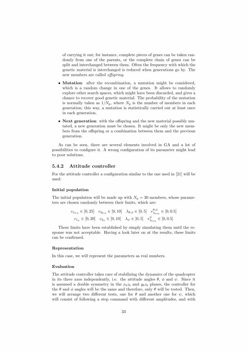
of carrying it out; for instance, complete pieces of genes can be taken ran-domly from one of the parents, or the complete chain of genes can besplit and interchanged between them. Often the frequency with which thegenetic material is interchanged is reduced when generations go by. Thenew members are called offspring.

• Mutation: after the recombination, a mutation might be considered,which is a random change in one of the genes. It allows to randomlyexplore other search spaces, which might have been discarded, and gives achance to recover good genetic material. The probability of the mutationis normally taken as 1/Np, where Np is the number of members in eachgeneration; this way, a mutation is statistically carried out at least oncein each generation.

• Next generation: with the offspring and the new material possibly mu-tated, a new generation must be chosen. It might be only the new mem-bers from the offspring or a combination between them and the previousgeneration.

As can be seen, there are several elements involved in GA and a lot ofpossibilities to configure it. A wrong configuration of its parameter might leadto poor solutions.

5.4.2 Attitude controller

For the attitude controller a configuration similar to the one used in [21] will beused:

Initial population

The initial population will be made up with Np = 30 members, whose parame-ters are chosen randomly between their limits, which are:

c1θ,φ ∈ [0, 25] c2θ,φ ∈ [0, 10] λθ,φ ∈ [0, 5] eθ,φλlim ∈ [0, 0.5]

c1ψ ∈ [0, 20] c2ψ ∈ [0, 10] λψ ∈ [0, 5] eψλlim ∈ [0, 0.5]

These limits have been established by simply simulating them until the re-sponse was not acceptable. Having a look later on at the results, these limitscan be confirmed.

Representation

In this case, we will represent the parameters as real numbers.

Evaluation

The attitude controller takes care of stabilizing the dynamics of the quadcopterin its three axes independently, i.e. the attitude angles θ, φ and ψ. Since itis assumed a double symmetry in the xbzb and ybzb planes, the controller forthe θ and φ angles will be the same and therefore, only θ will be tested. Then,we will arrange two different tests, one for θ and another one for ψ, whichwill consist of following a step command with different amplitudes, and with

33

time [s]0 5 10 15 20 25 30 35 40

θ [r

ad]

-0.05

0

0.05

0.1

0.15

0.2

θ

θc

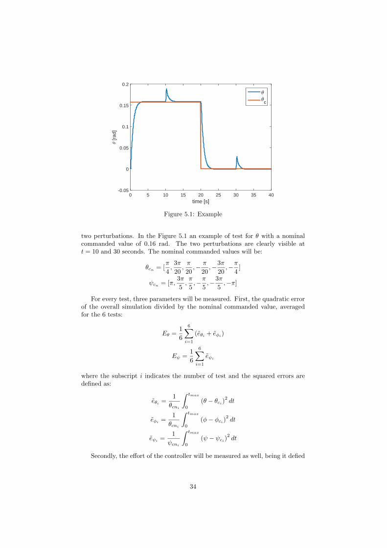
Figure 5.1: Example

two perturbations. In the Figure 5.1 an example of test for θ with a nominalcommanded value of 0.16 rad. The two perturbations are clearly visible att = 10 and 30 seconds. The nominal commanded values will be:

θcn = [π

4,

3π

20,π

20,− π

20,−3π

20,−π

4]

ψcn = [π,3π

5,π

5,−π

5,−3π

5,−π]

For every test, three parameters will be measured. First, the quadratic errorof the overall simulation divided by the nominal commanded value, averagedfor the 6 tests:

Eθ =1

6

6∑i=1

(eθi + eφi)

Eψ =1

6

6∑i=1

eψi

where the subscript i indicates the number of test and the squared errors aredefined as:

eθi =1

θcni

∫ tmax

0

(θ − θci)2dt

eφi =1

θcni

∫ tmax

0

(φ− φci)2dt

eψi =1

ψcni

∫ tmax

0

(ψ − ψci)2dt

Secondly, the effort of the controller will be measured as well, being it defied

34

as:

σθ =1

6

6∑i=1

∫ tmax

0

u2θi + u2φiθcni

dt

σψ =1

6

6∑i=1

∫ tmax

0

u2ψiψcni

dt

being uθi , uφi and uψi the control commands already shown.Finally, for high values of the parameters, one can realize that the kickback

phenomenon may appear, which is a return in the controlled value before havingreached the desired value. Moreover, with those high values, also high frequencyoscillations might also show up. To penalize these situations, another measure-ment value will be used, kb, which is the number of zeros in the derivative ofthe angle, being they closer than 0.2 seconds one from each other. Also, we willpenalize the overshooting by adding one unit to kb for every 2% of overshootingif it is higher than 5%; otherwise, no penalty will be applied.

We need to integrate all three measure values in one fitting variable. Letsdefine firstly a sub-fitting variable for each performance variable and for eachmember m of the population p:

fmE =min(Ep)

Em

fmσ =min(σp)

σm

fmkb =min(kb)

kbm

In the above expression, it was not explicitly written either θ nor ψ sincethey are valid for both variables. The operator min() is the minimum value of

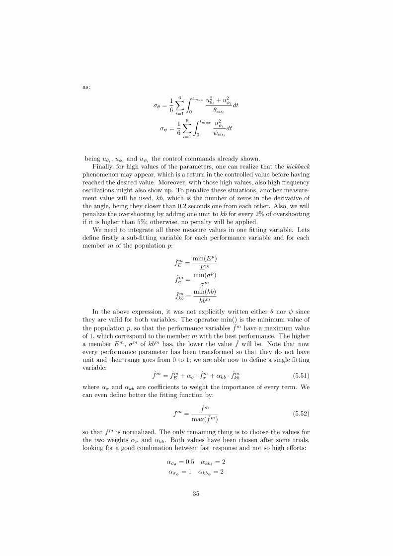
the population p, so that the performance variables fm have a maximum valueof 1, which correspond to the member m with the best performance. The highera member Em, σm of kbm has, the lower the value f will be. Note that nowevery performance parameter has been transformed so that they do not haveunit and their range goes from 0 to 1; we are able now to define a single fittingvariable:

fm = fmE + ασ · fmσ + αkb · fmkb (5.51)

where ασ and αkb are coefficients to weight the importance of every term. Wecan even define better the fitting function by:

fm =fm

max(fm)(5.52)

so that fm is normalized. The only remaining thing is to choose the values forthe two weights ασ and αkb. Both values have been chosen after some trials,looking for a good combination between fast response and not so high efforts:

ασθ = 0.5 αkbθ = 2

ασψ = 1 αkbψ = 2

35

Selection

Given a fitting value fm for every member, the roulette wheel method will beused to create the matting pool, which will be composed by a number of pairsequal to the size of the population (Np = 30). These pairs will be chosenfrom the previous generation randomly, taking into account a probability whichdepends on the fitting value fm as follows:

Pm =fm

Np∑i=1

f i(5.54)

One parent will not be allowed to be matched with itself and the same pairin the matting pool will be avoid either. It must be pointed out, that there willbe two independent matting pool, one for the θ variable and another one for ψ.

Recombination

For every pair of parents from the matting pool (recall that there are two), andfor every parameter of the solution, one will be taken randomly from one parentto form the next generation. We will then obtain Np new solutions after therecombination.

Although this method was the one used in [21], the new material which isintroduced in the generation is very small, since the recombination only takesthe material from one of the parents. One realizes after some simulations thatthe complete generation tends to converge to a few different members.

Another recombination is proposed, which consists of making an weightedaverage of both parents:

κoff = r · κ1 + (1− r) · κ2 (5.55)

where κi is the parameter of the parent i and r is a random number between0 and 1. This new method produces generations with members much moredifferent between them.

Mutation

For every parameter, there will be a probability of Pmut = 1/Np to be mutated;this value is often taken so statistically is ensured, that in every generation therewill be at least one mutation in every parameter. If the mutation takes place,it will happen as follows:

κ′ = κ+ sign(0.5− r1) · κmax2· r2 (5.56)

where r1 and r2 are two random number. If κ′ turns out to be negative, theprevious equation will be again calculated with new random parameters until itbecomes positive.

Next generation

The next generation will be made up with the best Np members of the previousgeneration and the offspring generated from them.

36

Config. c1 c2 λ eλlim E σ kb f

θ,φ

1 24.1 2.92 2.73 0.10 0.194 9.68 0.167 12 6.30 4.43 4.80 0.01 0.210 3.68 0.167 0.9853 15.9 2.59 0.78 0.06 0.235 4.64 0.167 0.9494 4.74 4.99 0.31 0.22 0.250 2.25 0.167 0.948

ψ

1 2.92 0.058 0.036 0.087 4.23 9.46 0.167 12 3.31 0.058 0.036 0.192 4.38 10.55 0 0.9663 3.92 0.007 0.267 0.182 4.55 12.9 0.167 0.9154 3.44 0.176 0.072 0.242 3.67 15.9 0 0.910

Table 5.1: Parameters of the best 4 configurations found by the genetic algo-rithm, with their quadratic error E, effort σ and kickback measurement kb.

The above configuration will be run a maximum of 50 generations, beingstopped if in 5 generations in a row, there is not an improvement in the bestmember of a 5%. Four different simulations will be carried out, two with therecombination proposed in [21] and two more with the recombination based onthe weighted average of the two parents.

In the Table 3.1 the parameters of the four best configurations found by thegenetic algorithm for the θ/φ and for the ψ controller have been presented. Alsothe values of the quadratic error E, the effort σ and the kickback number kbhaven also written, with the relative fitting value f . Note that configuration areordered so that the Configuration 1 is the best and the 4 is the worst.

The solutions for the controller of θ and φ are quite different between them,although the final result is very similar. The configuration 1 has a very high c1value so the effort is much higher than in the other configurations. Note thatfor the four configurations there is at least a kickback in one of the 6 test, beingthe kb = 1/6 = 0.167. On the other hand, the parameters for the ψ controllerare more similar between them, although the results are not.

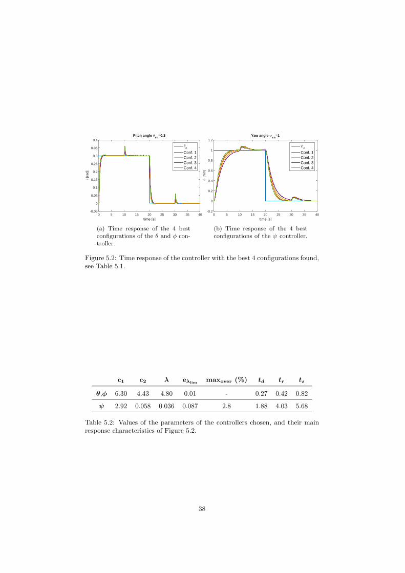
In the Figure 5.2 the time response of both controllers, with their four config-urations, have been represented for an nominal input of θcn = 0.3 and ψcn = 1rad. In the case of the pitch angle, see Figure 5.2a, configurations 1 and 2 arevery similar and the only clearly visible difference is that in presence of a pertur-bation, configuration 1 returns to the reference value faster and therefore, theerror is lower, see Table 5.1. However, configuration 1 needs a way higher effortand the likelihood of that the kickback shows up is also higher. Therefore, con-figuration 2 will be chosen. On the other hand, for the angle ψ, Figure 5.2b, itcan be seen that configuration 4 is the best results in terms of velocity responseand error and it has not overshooting; however, it requires much more effort andsince the yaw control is not a relevant nor critical operation, it could preventthe θ and φ controller to fulfill their duties in the best possible way. Because ofthis, configuration 4 has been discarded and configuration 1 has been chosen,which still has a fast response with a slight overshooting, but it requires lesscontrol effort.

The parameters of the controllers chosen, with their main response charac-teristics, have been presented in Table 5.2. The percentage of overshooting, thedelay time td, the rise time, tr and the settling time ts, all in seconds, have beencalculated having as a reference response the one shown in Figure 5.2.

37

time [s]0 5 10 15 20 25 30 35 40

θ [r

ad]

-0.05

0

0.05

0.1

0.15

0.2

0.25

0.3

0.35

0.4Pitch angle θ

cn=0.3

θc

Conf. 1Conf. 2Conf. 3Conf. 4

(a) Time response of the 4 bestconfigurations of the θ and φ con-troller.

time [s]0 5 10 15 20 25 30 35 40

ψ [r

ad]

-0.2

0

0.2

0.4

0.6

0.8

1

1.2Yaw angle ψ

cn=1

ψc

Conf. 1Conf. 2Conf. 3Conf. 4

(b) Time response of the 4 bestconfigurations of the ψ controller.

Figure 5.2: Time response of the controller with the best 4 configurations found,see Table 5.1.

c1 c2 λ eλlim maxover (%) td tr ts

θ,φ 6.30 4.43 4.80 0.01 - 0.27 0.42 0.82

ψ 2.92 0.058 0.036 0.087 2.8 1.88 4.03 5.68

Table 5.2: Values of the parameters of the controllers chosen, and their mainresponse characteristics of Figure 5.2.

38

5.4.3 Position Controller

In the case of the position controller, there are more parameters to be deter-mined. Also, there are more elements involved in the movement; not only aposition must be reached, but also the perturbation D and the mass m must beestimated by different tests. As done with the attitude controller, the followingelements of the GA will be taken into consideration.

Initial population

The initial population will be taken randomly between a range of values, deter-mined after some trials:

c1x,y ∈ [0, 5] λx,y ∈ [0, 2] ex,yλlim ∈ [0, 0.1] kx,y ∈ [0, 5]

γx,y ∈ [0, 1] β1x,y ∈ [0, 2] β2x,y ∈ [0, 0.5] β3x,y ∈ [0, 5]

λz ∈ [0, 0.5] ezλlim ∈ [0, 1] γ1z ∈ [0, 0.1]

γ2z ∈ [0, 0.1] c1z ∈ [0, 0.5] c2z ∈ [0, 2]

We will use again Np = 30 members. Since this controller is specially com-plicated to be tuned, its likely that the first generations are made up with verybad solutions. Therefore, 5 solutions with good performance will be included inthe initial population.

Representation

Again, the parameters will be represented as real numbers.

Evaluation

The performance of the controller of the x and y direction will be tested bycommanding different positions in the x direction, keeping altitude and positionalong y direction. Also, different perturbation forces will be applied to thequadcopter. The complete sequence of action to test the horizontal positioncontroller is:

1. Wait 2 second to stabilize the quadcopter in the z direction.

2. Go forward 1 m.

3. Go backward 2 m.

4. Go forward 7 m.

5. Go backward 13 m.

6. Go forward 23 m.

7. Go backward 33 m.

8. Go forward 10 m. back to the initial position.

9. Apply a perturbation force of 1 N.

10. Apply a perturbation force of 2 N.

39

11. Reduce the perturbation force to 0.5 N.

In case of the vertical position controller, the position and a perturbationwill be tested, but also a change in the mass. It must be remarked that achange in the mass will imply a vertical force in the zb direction and thereforethe controller must interpreter as a perturbation Dz. This means that whenevaluating the ability of the controller to identify a change in the mass, theperturbation estimation must be disable, and the other way around. Two testwill be carried out

The first test, to evaluate the altitude change and the ability of detectingvertical perturbations:

1. Disable the detection of the mass change.

2. Wait 2 second to stabilize the quadcopter in the z direction.

3. Ascend 1 m.

4. Ascend 5 m.

5. Ascend 20 m.

6. Descend 20 m.

7. Descend 5 m.

8. Descend 1 m, back to the initial position.

9. Apply a perturbation force of 2 N in the zb direction.

10. Apply a perturbation force of 4 N.

11. Reduce the perturbation force to 1 N.

12. Remove the perturbation.

The second test, to evaluate the ability of detecting changes in the mass ofthe quadcotper:

1. Disable the detection of the perturbation.

2. Change the mass of the quadcopter to m0 + 0.150 kg.

3. Change the mass of the quadcopter to m0 + 0.300 kg.

4. Change the mass of the quadcopter to m0 − 0.150 kg.

5. Change the mass of the quadcopter to m0 − 0.300 kg.

It must be pointed out that we might have proposed different experimentsto determined the best parameters solution for the m and D, and afterwardsother experiment to best fit the remaining parameters. However, we would thenchoose some parameters taking into account only the m and D estimation, andthen they might not be appropriate for the quadcopter’s movement, since thecontroller depends directly on them.

40

To evaluate the performance of the controller, as similar approach made forthe attitude controller will be done. On one hand, we will consider the quadraticerror, define as:

Ex =

∫ tmax

0

(x− xc)2dt+

∫ tmax

0

y2dt

Ez =

∫ tmax

0

(z − zc)2dt

On the other hand, the effort will be also considered in the same way it wasdone for the attitude controller:

σx =

∫ tmax

0

(u2x + u2y)dt

σz =

∫ tmax

0

(u1 −m0 · g)2dt

where in the vertical effort the weight has been subtracted to better representthe effort to change the altitude.

Although a slow or bad estimation of the D or m would imply higher er-rors and efforts, it is convenient to also consider them separately in the finalevaluation function by the following variables:

EDx =

∫ tmax

0

D2xdt

EDz =

∫ tmax

0

D2zdt

Em =

∫ tmax

0

m2dt

Since both controllers, especially the zb one, present easily overshoot, anotherevaluating variable will be included:

Eover =

{0 if maxover ≤ 5%100 ·maxover − 5 if maxover > 5%

(5.61)

Here the maxover accounts the addition of the total overshooting in every stepof the reference signals.

The fitting function will be composed as it was done for the attitude con-troller:

fmE =min(Ep)

Em

fmσ =min(σp)

σm

fmED =min(Ep

D)

EmD

fmEm =min(Epm)

Emm

fmover =1 + min(Epover)

max (Emover, 1)

41

where p refers to the complete population and m only the member under study.All the fitting functions will be included in a single value:

fmx = fmEx + ασx · fmσx + αDx · fmEDx

+ αoverx · fmoverxfmz = fmEz + ασz · fmσz + αDz · f

mEDz

+ αm · fmEm + αoverz · fmoverz

and finally the fitting value of each member can be change so that the maximumvalue is 1:

fmx =fmx

max(fmx )

fmz =fmz

max(fmz )

The values of the proportional parameters to evaluate the fitting value willbe taken as:

ασx = 0.5 αDx = 2.5 αoverx = 1.5

ασz = 0.5 αDz = 1.5 αm = 1.5 αoverz = 2

Selection, recombination and next generation

All three will be carried out same way as it was done for the attitude controller.

Once the evaluation has been established, the algorithm is run for a maxi-mum of 50 generations, being stopped if the improvement is lower than 5% in5 generations in a row. Several simulations are carried out, and from each onethe best members are taken and used in the next simulations. It is relativelyeasy to find acceptable solutions for the x and y controller, but not for the zcontroller, which is more sensitive to the parameters.

In Table 5.3 the best 4 configuration have been taken and their evaluatingvalues presented. The configurations of the x and y axes are very similar,since the values of the fitting function f are all close to 1. Having a look atthe response, configuration 3 will be taken, since its able to absorb faster theperturbations Dx. The case of the altitude controller is different, since thereis a remarkable difference between the best configuration and the second one;configuration 1 will be selected then.

The values of all parameters will be then:

c1x,y = 0.813 λx,y = 1.53 ex,yλlim = 0.152 kx,y = 2.39

γx,y = 0.435 β1x,y = 0.196 β2x,y = 0.140 β3x,y = 1.54

λz = 0.0010 ezλlim = 0.143 γ1z = 0.219

γ2z = 3.21 c1z0.819 c2z = 4.93

In Figure 5.3 the system response, for the planned test, has been represented,with the configurations selected; the reference signals and the true values are inblue, and in red the real and estimated values. The first two figures correspondto the test in the xb direction, whereas the other three correspond to the altitudecontroller and the estimation of the mass.

42

Config. E σ ED Em Eover f

x,y

1 1488 3.33 56.0 - 0.98 12 1535 2.86 59.7 - 0 0.983 1498 3.12 67.9 - 0.12 0.944 1475 3.29 37.1 - 23.0 0.87

z

1 222 1933 67.6 0.113 0 12 211 1796 58.5 0.125 6.21 0.743 221 1689 63.4 0.115 27.5 0.694 224 1582 60.8 0.155 27.1 0.64

Table 5.3: Parameters of the best 4 configurations found by the genetic algo-rithm, with their quadratic error E, effort σ and kickback measurement kb.

In Figure 5.3a the movement in the xb direction can be seen; the quadcopteris able to follow the reference signals successfully with a slight overshooting.When the reference signal is zero, from t = 70 s on, the movements due to theperturbations are visible, although the quadcopter comes back to the desiredposition rapidly. In Figure 5.3b the perturbation in the xb direction has beenrepresented, as well as the estimated value. When a reference xb value is com-manded, the algorithm estimates a perturbation which actually does not exist;furthermore, when the perturbation actually exists, the algorithm needs longtimes to approach the final value, see convergence to the step values. Althoughthe estimation seems to not work properly, the fact is that the controller absorbsthem properly.

In Figure 5.3c the movement in the zb direction has been represented. As ithappened with the horizontal controller, the reference value is followed withoutproblem and without overshooting. The perturbations due to Dz are also wellabsorbed. This controller is more capable of estimating the perturbation, ascan be seen in Figure 5.3d. Finally, in Figure 5.3e the estimation of the masshas been shown. The algorithm estimates fast and accurately the real mass ofthe quadcopter; it must be pointed out, that in this test, there is no changeof altitude and the perturbation estimation in the zb direction, Dz, has beendisabled.

As already indicated, the mass and the vertical perturbation estimationmight be misinterpreted by the algorithm; a change in the mass can be seenas an addition of a vertical force, and the other way around. Actually, when achange of altitude is commanded, Dz and m become non-zero. Since the massis not expected to change during the flight, the mass estimation will be only ac-tivated during a short time in the beginning of the flight, while the quadcopterhovers at a certain altitude; once the mass has been calculated, we will force˙m = 0. Keeping in mind the result of Figure 5.3e, the estimation might need

less than 5 s.The configuration already defined will be tested with the same trajectory in

Figure 4.4a. Initially, the quadcopter is grounded and the mass is increased in0.3 kg, so that the controller estimates it after taking off. Also, a perturbationof 2 N will be afterwards applied in xb and yb axes, at t =45 and 65 s, and of 3N in the zb direction at t =85 s. In Figure 5.4a, the position of the quadcopterhas been represented, in dotted lines the reference values and solid lines the

43

time [s]0 20 40 60 80 100 120 140 160

X [m

]

-10

-8

-6

-4

-2

0

2

4

6

8

10 Xr

X

(a) Movement in the xb direction.

time [s]0 20 40 60 80 100 120 140 160

Dx[N

]-3

-2

-1

0

1

2

3

Dx

Dx

(b) Estimation of the perturbationDx.

time [s]0 20 40 60 80 100 120 140 160

Z [m

]

-26

-24

-22

-20

-18

-16

-14

-12

-10

Zr

Z

(c) Movement in the zb direction.

time [s]0 20 40 60 80 100 120 140 160

Dz[N

]

-5

-4

-3

-2

-1

0

1

2

3

4

5

Dz

Dz

(d) Estimation of the perturba-tion Dx.

time [s]0 5 10 15 20 25 30

m[kg]

1

1.1

1.2

1.3

1.4

1.5

1.6

1.7

1.8

m

mz

(e) Estimation of the mass m.

Figure 5.3: Result of the tests with configuration 3 for the controller in the xband yb direction and controller 1 in the zb direction.

44

Characteristic x, y z

maxover (%) 6 -td(s) 1.05 0.81tr 1.52 2.14ts 3.42 3.28

Table 5.4: Time characteristics of the two nonlinear controllers of the horizontaland vertical positioning, with reference values x = 1 m and z = −1 m.

actual values. The controller is able to absorb firstly the excess of mass in thefirst seconds, and afterwards the disturbances on every axes.

In Figure 5.4b the disturbances on the quadcopter and their estimation havebeen represented. The three estimation remain close to the zero value until theperturbations take place at 45, 65 and 85 s. The estimated values convergeapproximately to the real values; although the approximation is not perfect, thecontroller absorbs the perturbation, as can be seen in Figure 5.4a.

Finally, in Figure 5.4c the mass estimation and its real value has been shown.Within 6 seconds, the algorithm estimates perfectly the real mass of the quad-copter; afterwards, the mass estimation is disable and the final value used fromthen on. The take off of the quadcopter delays the convergence of the estimation;if we had considered that the quadcopter was already hovering, the convergencewould have taken place in less than 2 s. Once the mass has been estimated, itsvalue it passed to the x and y controller, see Equation 5.2; the update of thevalue improves remarkably the performance of the position control, speciallywhen absorbing external perturbations.

It must be remark that the result here achieve seem to be better than thoseobtained in [9]. Of course the quadcopter model is different and the final valuesof the parameters are not specified, but the results present overshooting, highoscillations and irregularities. The method there used to choose the parametersis not specified.

45

time [s]0 20 40 60 80 100 120

Pos

ition

[m]

-1.5

-1

-0.5

0

0.5

1

1.5

XYZ

(a) Position of the quadcopter.

time [s]0 20 40 60 80 100 120

D

-3

-2

-1

0

1

2

3

Dx

Dx

Dx

(b) Estimation of the perturba-tions.

time [s]0 1 2 3 4 5 6

m

1.4

1.45

1.5

1.55

1.6

1.65

1.7

1.75

1.8

(c) Estimation of the mass m dur-ing the first 5 seconds.

Figure 5.4: Test with the final configuration of the controller, similar to the onein Figure 4.4a, but with a change of +0.3 kg in the mass and perturbations inthe three axes.

46

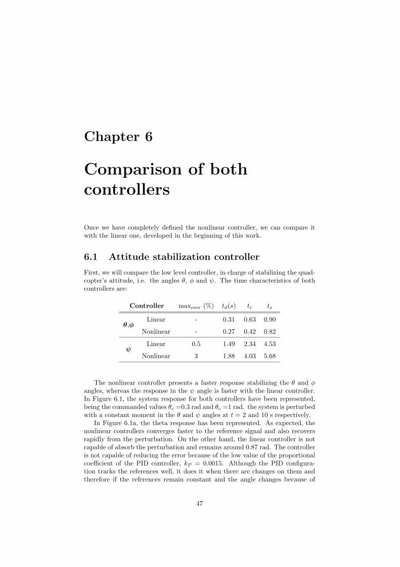
Chapter 6

Comparison of bothcontrollers

Once we have completely defined the nonlinear controller, we can compare itwith the linear one, developed in the beginning of this work.

6.1 Attitude stabilization controller

First, we will compare the low level controller, in charge of stabilizing the quad-copter’s attitude, i.e. the angles θ, φ and ψ. The time characteristics of bothcontrollers are:

Controller maxover (%) td(s) tr ts

θ,φLinear - 0.31 0.63 0.90

Nonlinear - 0.27 0.42 0.82

ψLinear 0.5 1.49 2.34 4.53

Nonlinear 3 1.88 4.03 5.68

The nonlinear controller presents a faster response stabilizing the θ and φangles, whereas the response in the ψ angle is faster with the linear controller.In Figure 6.1, the system response for both controllers have been represented,being the commanded values θc =0.3 rad and θc =1 rad. the system is perturbedwith a constant moment in the θ and ψ angles at t = 2 and 10 s respectively.

In Figure 6.1a, the theta response has been represented. As expected, thenonlinear controllers converges faster to the reference signal and also recoversrapidly from the perturbation. On the other hand, the linear controller is notcapable of absorb the perturbation and remains around 0.87 rad. The controlleris not capable of reducing the error because of the low value of the proportionalcoefficient of the PID controller, kP = 0.0015. Although the PID configura-tion tracks the references well, it does it when there are changes on them andtherefore if the references remain constant and the angle changes because of

47

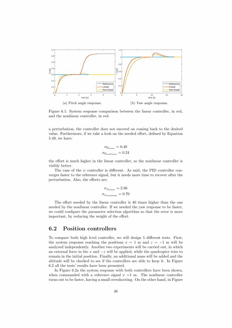
time [s]0 1 2 3 4 5

θ [r

ad]

0

0.1

0.2

0.3

0.4

0.5

0.6

0.7

ReferenceLinealNon-lineal

(a) Pitch angle response.

time [s]0 5 10 15 20

ψ [r

ad]

0

0.2

0.4

0.6

0.8

1

1.2

ReferenceLinealNon-lineal

(b) Yaw angle response.

Figure 6.1: System response comparison between the linear controller, in red,and the nonlinear controller, in red.

a perturbation, the controller does not succeed on coming back to the desiredvalue. Furthermore, if we take a look on the needed effort, defined by Equation5.49, we have:

σθlinear = 0.40

σθnonlinear = 0.24

the effort is much higher in the linear controller, so the nonlinear controller isvisibly better.

The case of the ψ controller is different. As said, the PID controller con-verges faster to the reference signal, but it needs more time to recover after theperturbation. Also, the efforts are:

σψlinear= 2.86

σψnonlinear= 0.70

The effort needed by the linear controller is 40 times higher than the oneneeded by the nonlinear controller. If we needed the yaw response to be faster,we could configure the parameter selection algorithm so that the error is moreimportant, by reducing the weight of the effort.

6.2 Position controllers

To compare both high level controller, we will design 5 different tests. First,the system response reaching the positions x = 1 m and z = −1 m will beanalyzed independently. Another two experiments will be carried out, in whichan external force in the x and −z will be applied, while the quadcopter tries toremain in the initial position. Finally, an additional mass will be added and thealtitude will be checked to see if the controllers are able to keep it. In Figure6.2 all the tests’ results have been presented.

In Figure 6.2a the system response with both controllers have been shown,when commanded with a reference signal x =1 m. The nonlinear controllerturns out to be faster, having a small overshooting. On the other hand, in Figure

48

6.2b the movement in the zb axes can be seen, being initially the quadcoptergrounded and taking off to an altitude of z = −1 m. In this case, the linearcontroller is faster than the nonlinear one. The time domain characteristics ofboth controllers, in both axes are the following:

Controller maxover (%) td(s) tr ts

x,yLinear 0 1.58 3.72 5.51

Nonlinear 6 1.05 1.52 3.42

zLinear 0 0.41 1.00 1.55

Nonlinear 0 0.81 2.14 3.28

It should be remarked that the PID controller in the zb is 2 times faster thanthe nonlinear controller, which is an important advantage. The effort turns outto be:

σzlinear = 2081

σznonlinear = 1904

Both controllers need almost the same effort. If we define now the effort toreach a position in the x direction as:

σx = σθ =

∫ t

0

uθ · dt (6.4)

the effort of both controller to reach the [1,0] position are:

σxlinear= 0.104

σxnonlinear= 2.053

The nonlinear controller need 20 times more effort to reach the desired po-sition.

In Figure 6.2c, an external force of 2 N in the x direction has been applied,being shown the position along this axis. The lineal controller is not able toabsorb the force and come back to the initial position; only after 25 s, when thequadcopter reaches x = 10.5 m, the error term of the backstepping controllerin high enough to counteract the perturbation and the quadcopter starts slowlyreturning to the initial position (not shown in the figure). On the other hand,the nonlinear controller absorbs the perturbation in within 9 s, keeping thequadcopter closer than 30 cm from the required position.

The situation when applying a vertical force Dz is similar, but the linearcontroller is not able to return to the initial position and only keeps the altitudeat z = −1.6 m (note that the direction of the force is zb). On the contrary, thenonlinear controller returns slowly to the reference altitude, and also avoids thequadcopter to increase its altitude more than 0.25 m.

Finally, if an additional mass is added to the quacopter, the nonlinear con-troller estimates it successfully and returns to the desired altitude in less than2 s, as can be seen in Figure 6.2e. As it happened when adding an external ver-tical force, the linear controller can not absorb it and the quadcopter decreasesthe altitude because of the additional mass down to 0.42 cm.

49

time [s]0 2 4 6 8 10

X [m

]

0

0.2

0.4

0.6

0.8

1

1.2

ReferenceLinealNon-lineal

(a) Movement in the x direction.

time [s]0 2 4 6 8 10

Z [m

]

-1

-0.8

-0.6

-0.4

-0.2

0

0.2

ReferenceLinealNon-lineal

(b) Movement in the zb direction.

time [s]0 2 4 6 8 10

X [m

]

0

1

2

3

4

5

6

7

ReferenceLinealNon-lineal

(c) Movement in the x directionwith non zero Dx.

time [s]0 2 4 6 8 10

Z [m

]

-1.6

-1.5

-1.4

-1.3

-1.2

-1.1

-1

-0.9

ReferenceLinealNon-lineal

(d) Movement in the zb directionwith non zero Dz.

time [s]0 2 4 6 8 10

Z [m

]

-1.1

-1

-0.9

-0.8

-0.7

-0.6

-0.5

-0.4

ReferenceLinealNon-lineal

(e) Movement in the zb directionwith an additional mass.

Figure 6.2: Comparison of the system position response in the five differentcases considered.

50

6.3 Conclusions

In this master thesis, an analysis of the dynamics of the quadcopter has beenfirstly carried out. The first controller, whose design has been based on a lin-earized model, has been developed for the 3dof and 6dof quadcopter. A goodperformance has been achieved, even when tested with a non-linear model. How-ever, taking a look on the inputs to the electric motors (see Figure (4.5b)), itlooks like that they might be more demanding in order to make the move-ments faster and in general to make the quadcopter agiler. Moreover, a somenon-realistic behaviors have been assumed, as signals without noise and no aero-dynamic forces and moments.

Afterwards, another PID controller has been proposed to stabilize the atti-tude of the six degrees of freedom model, keeping in mind that the parametersof the model (mass, inertia, etc.) are different. The position control is then con-structed by using the backstepping method, obtaining a second order system(Equations 4.5) whose convergence is ensured.

To improve the controller, a similar one is in Chapter 5 presented. This hasa more complex control laws so that external forces and changed in the massare considered. The convergence is proved by using Lynapunov functions. Thedrawback of this controller is that it is not easy to tune, as it has been seen,since it has a high number of parameters to be chosen. A genetic algorithmhas been selected to set the parameters, considering some goals for the systemresponse (system response, overshooting, kick-back behavior, mass and distur-bance estimation, etc.). The final controller is able to successfully estimatechanges in the mass faster than perturbations, being the desired behavior theother way around, since external forces, such as wind gusts, might change faster.Therefore, only constant, or slow changing, perturbations can be successfullyestimated, such as discrepancies with the model.

Finally, both controllers are compared with different tests. In the case of theattitude stabilization, having a look at the time characteristics of the systemresponse, it has been shown that the nonlinear controller is faster than the linearone; on the other hand, the yaw control is faster with the linear one, althoughit requires way more effort, approximately 40 times more. Also a perturbationhas been applied in every axes to check the ability to absorb it; the nonlinearcontroller recovers the desired input, while the linear controller is not able torecover it for the attitude angles and for the yaw angles it does, but slower.

For the position control, a comparison of the characteristic time has been alsoshown. In the case of horizontal positioning, the nonlinear controller is faster(the rise time is more than two times shorter) but it needs much more effort.To control the vertical movement, the linear controller shows faster responseswith approximately the same effort. The rejection of external forces is almostnonexistent with the linear controller, whereas the nonlinear one absorbs themsuccessfully. The same situation takes place when there is a change in themass of the quadcopter; the nonlinear controller can execute the estimationof the mass once it takes off and after 5 seconds the mass will be accuratelyapproximated, and afterwards this term can be disable since no further masschanges is expected.

As can be seen, the nonlinear controller presents clear advantages over thelinear one. Moreover, we could have checked other robustness indicators, byassuming another discrepancies between the model and the real system, such

51

us changes in the inertial moments, motor responses or propeller misalignment.If these factors are required to be considered, the genetic algorithm, used totune the controller, might take them into account with more tests and weightedin the fitting function. Any other system response characteristic might also beconsidered, modeled and included in the evaluation of each function (such asmaximum rotation speed). This is the main advantage of the here presentedcontroller, the freedom of adapting the configuration depending on the require-ments asked to the system. It is important to remark that the more complexthe requirements, or the more number of requirements are needed, the moredifficult the tuning of the GA is, by setting the wights of each characteristic.

52

Appendix A

Simulink models

A.1 3dof quadcopter parameters

Parameter Value

m 2.85 kgd 0.1969 mdN

1 0.0182 mIx 0.0552 kg·m2

Iy 0.0552 kg·m2

Iz 0.1104 kg·m2

ωm 100/15 rad/sµ 0.5940 N/Vg 9.8 m/s2

Vmax 22 VVmin 0 Vpmaxqmax ±40◦/srmax

1Note that the relationship between forces and yaw moment and the voltage to be suppliedto the engines is different from how they are described in the exercise formulation, having nowµ = K and dN = K2/K.

53

A.2 6dof quadcopter parameters

Parameter Value

m 1.40 kgd 0.20 mdN 0.03 mIx 0.03 kg·m2

Iy 0.03 kg·m2

Iz 0.042 kg·m2

ωm 15 rad/sµ 1 N/Vg 9.8 m/s2

Vmax 20 VVmin 0 Vpmaxqmax ±40◦/srmax

54

Bibliography

[1] Adamy, J. (2005). Implicit Lyapunov functions and isochrones of linear sys-tems. IEEE Transactions on Automatic Control, 50(6), 874-879.

[2] Argentim, L. M., Rezende, W. C., Santos, P. E., & Aguiar, R. A. (2013,May). PID, LQR and LQR-PID on a quadcopter platform. In Informatics,Electronics & Vision (ICIEV), 2013 International Conference on (pp. 1-6).IEEE.

[3] Bai, Y., Liu, H., Shi, Z., & Zhong, Y. (2012, July). Robust control of quadro-tor unmanned air vehicles. In Control Conference (CCC), 2012 31st Chinese(pp. 4462-4467). IEEE.

[4] Bouabdallah, S., & Siegwart, R. (2005, April). Backstepping and sliding-mode techniques applied to an indoor micro quadrotor. In Robotics andAutomation, 2005. ICRA 2005. Proceedings of the 2005 IEEE InternationalConference on (pp. 2247-2252). IEEE.

[5] Bouffard, P. (2012). On-board Model Predictive Control of a Quadrotor He-licopter: Design, Implementation, and Experiments (No. UCB/EECS-2012-241). CALIFORNIA UNIV BERKELEY DEPT OF COMPUTER SCI-ENCES.

[6] Chen, B. S., Cheng, Y. M., & Lee, C. H. (1995). A genetic approach tomixed H2/H∞ optimal PID control. Control Systems, IEEE, 15(5), 51-60.

[7] Diao, C., Xian, B., Yin, Q., Zeng, W., Li, H., & Yang, Y. (2011, May). Anonlinear adaptive control approach for quadrotor UAVs. In Control Con-ference (ASCC), 2011 8th Asian (pp. 223-228). IEEE.

[8] Dierks, T., & Jagannathan, S. (2010). Output feedback control of a quadro-tor UAV using neural networks. Neural Networks, IEEE Transactions on,21(1), 50-66.

[9] Fang, Z., & Gao, W. (2011, July). Adaptive integral backstepping control ofa micro-quadrotor. In Intelligent Control and Information Processing (ICI-CIP), 2011 2nd International Conference on (Vol. 2, pp. 910-915). IEEE.

[10] Fatan, M., Sefidgari, B. L., & Barenji, A. V. (2013, August). An adap-tive neuro PID for controlling the altitude of quadcopter robot. In Methodsand Models in Automation and Robotics (MMAR), 2013 18th InternationalConference on (pp. 662-665). IEEE.

55

[11] Fleming, P. J., & Purshouse, R. C. (2002). Evolutionary algorithms incontrol systems engineering: a survey. Control engineering practice, 10(11),1223-1241.

[12] Giagkiozis, I., & Fleming, P. J. (2015). Methods for multi-objective opti-mization: An analysis. Information Sciences, 293, 338-350.

[13] Hably, A., Kendoul, F., Marchand, N., & Castillo, P. (2006). Further resultson global stabilization of the PVTOL aircraft. Positive Systems, 303-310.

[14] Hoffmann, G. M., Huang, H., Waslander, S. L., & Tomlin, C. J. (2007, Au-gust). Quadrotor helicopter flight dynamics and control: Theory and exper-iment. In Proc. of the AIAA Guidance, Navigation, and Control Conference(Vol. 2).

[15] Huo, X., Huo, M., & Karimi, H. R. (2014). Attitude stabilization control ofa quadrotor UAV by using backstepping approach. Mathematical Problemsin Engineering, 2014.

[16] Lee, K. U., Kim, H. S., Park, J. B., & Choi, Y. H. (2012, October). Hoveringcontrol of a quadrotor. In Control, Automation and Systems (ICCAS), 201212th International Conference on (pp. 162-167). IEEE.

[17] Li, J., & Li, Y. (2011, August). Dynamic analysis and PID control fora quadrotor. In Mechatronics and Automation (ICMA), 2011 InternationalConference on (pp. 573-578). IEEE.

[18] NG TZE HUI, T. H. O. M. A. S. (2007). Design optimization of small-scaleunmanned air vehicles (Doctoral dissertation).

[19] Palunko, I., & Fierro, R. (2011, August). Adaptive control of a quadrotorwith dynamic changes in the center of gravity. In Proceedings 18th IFACWorld Congress (Vol. 18, No. 1, pp. 2626-2631).

[20] Santos, M., Lopez, V., & Morata, F. (2010, November). Intelligent fuzzycontroller of a quadrotor. In Intelligent Systems and Knowledge Engineering(ISKE), 2010 International Conference on (pp. 141-146). IEEE.

[21] Shen, J. C. (2002). New tuning method for PID controller. ISA transactions,41(4), 473-484.

[22] Sutarto, H. Y., Budiyono, A., Joelianto, E., & Hiong, G. T. (2006, Decem-ber). Switched linear control of a model helicopter. In Control, Automation,Robotics and Vision, 2006. ICARCV’06. 9th International Conference on(pp.1-8). IEEE.

[23] Yang, Z., & Pedersen, G. (2006, October). Automatic tuning of PID con-troller for a 1-D levitation system using a genetic algorithm-a real case study.In Computer Aided Control System Design, 2006 IEEE International Con-ference on Control Applications, 2006 IEEE International Symposium onIntelligent Control, 2006 IEEE (pp. 3098-3103). IEEE.

[24] Zulu, A., & John, S. (2014). A Review of Control Algorithms for Au-tonomous Quadrotors. Open Journal of Applied Sciences, 4(14), 547.

56