Control and optimization of the start-up of a combined cycle … · · 2013-03-05POLITECNICO DI...

POLITECNICO DI MILANO

Facolta di Ingegneria dell’Informazione

Corso di Laurea in Ingegneria dell’Automazione

Control and optimization of thestart-up of a combined cycle

power plant

Relatore: Candidato:Prof. Riccardo Scattolini Fabio Righetti, n°724560Correlatori:Ing. Damien FailleIng. Frans Davelaar

Anno Accademico 2009-2010

Io non ho talenti straordinari.Sono solo appassionatamente curioso

A. Einstein

Contents

1 Chapter 1: System Description and dynamic model 111.1 Physical system . . . . . . . . . . . . . . . . . . . . . . . . . . 11

1.1.1 The Gas Turbine system . . . . . . . . . . . . . . . . . 111.1.2 The Heat Recovery Steam Generator . . . . . . . . . . 191.1.3 Steam turbine stage . . . . . . . . . . . . . . . . . . . 281.1.4 Mixers and attemperators . . . . . . . . . . . . . . . . 321.1.5 Model of the thermo-mechanical stresses in the turbine

rotor . . . . . . . . . . . . . . . . . . . . . . . . . . . . 351.2 Plant data . . . . . . . . . . . . . . . . . . . . . . . . . . . . . 381.3 Modelica Model . . . . . . . . . . . . . . . . . . . . . . . . . . 41

2 Chapter 2: Identification of a simplified model 452.1 Identification approach: interpolation of linear models . . . . . 452.2 Selection of the operating points for identification . . . . . . . 482.3 Simulations on Dymola . . . . . . . . . . . . . . . . . . . . . . 49

2.3.1 Simulation at 100% of GT Load . . . . . . . . . . . . . 492.4 Identification with the Matlab Identification Toolbox . . . . . . 552.5 Building the interpolation scheme with Matlab Simulink . . . 60

3 Chapter 3: Validation of the identified models 65

4 Chapter 4: Optimization 824.1 Minimum-time optimization problem . . . . . . . . . . . . . . 824.2 Matlab Algorithm . . . . . . . . . . . . . . . . . . . . . . . . . 834.3 Optimization Results . . . . . . . . . . . . . . . . . . . . . . . 86

5 Chapter 5: Conclusion 92

A Simulations Procedure 94A.1 Simulations on Dymola . . . . . . . . . . . . . . . . . . . . . . 94A.2 Files manual . . . . . . . . . . . . . . . . . . . . . . . . . . . . 95

Ringraziamenti - Acknowledgements

Un sentito e doveroso ringraziamento va al Prof. Riccardo Scattolini, che miha dato, anzi regalato, la possibilita di svolgere questa Tesi, una esperienzache non avrei mai creduto possibile, oltre ad aver apportato il suo contributodove e quando era necessario, sempre con un clima di apertura e disponibilitache non e facile trovare. Voglio inoltre ringraziare il Prof. Francesco Casella,per i chiarimenti e le delucidazioni su Dymola e sul tipo di processo in esame.Ringrazio inoltre l’azienda Electricite de France (EDF) per la disponibilita el’accoglienza.

I would to thank Ing. Damien Faille for the opportunity to do this the-sis in EDF - Chatou. His contribute in this thesis was very important, evenhis agreeable company during Paris period. I want to thank also Ing. FransDavelaar for his attention and disponibility in every moment to solve myproblem. I couldn’t forget Adrian Tica for his total availability and his hugecontribute in this thesis to realize all the simulations I needed.In my Paris experience it’s impossible to forget Adrian’s company: withouthim my presence in France wouldn’t be the same thing. Especially I want tothank him for KFC experience and for the time passed together!I want also to thank other people in EDF: the others stagiaers (Fanny withher chair, Paula, PierAlban, David), Marite and Serge Moran, all the peopleof STEP group. Last but not the list, the group of FDM, that give me alittle injection of football in France.

Dopo i ringraziamenti ufficiali, che accompagnano ogni tesi (perche cosı egiusto, senza il contributo dei Prof. non se ne viene mai a campo in fondo)ci sono sempre quelli piu intensi, piu emozionanti, quelli personali...Il modo giusto per iniziarli? Credo questo...

Una vita da medianoa recuperar palloni

nato senza i piedi buonilavorare sui polmoni

una vita da medianocon dei compiti precisia coprire certe zone

a giocare generosi, lı,sempre lı

Si, questi anni sono stati una grande partita, senza magari piedi buoni, malavorando sulla corsa, sui polmoni, sul fare, sulla voglia di vincere (con un

4

pochino di doping dai... chiamiamoli cosı). Sudore, fatica, difficolta, ma an-che tanta gioia, tante persone incontrate, conosciute, vissute.Una grande partita... da commentare e ricordare, magari cosı...

Amici ascoltatori, ecco la formazione ufficiale: Federico, Ciro, Gabry, Maji,Giorgio. Essı perche sono stati loro la squadra che e scesa sempre in campoe che mi ha accompagnato in questa grande sfida.Federico, che da buon portiere parava le mie menate universitarie anche noncapendoci un tubo, sempre pronto a chiamarmi anche quando tra mille esami,scritti, orali e tesi facevo fatico a sentirlo. Piuttosto che perdermi e arrivatoa prendermi a pugni in piu e piu lezioni.Ciro che anche se viene e va, alla fine sempre e qua. Quando qualcosa nonquadra, quando bisogna lamentarsi, arrabbiarsi, ma soprattutto divertirsi,sdare... beh qualsiasi cosa ci sia da fare si sa sempre chi chiamare. Certo lepolemiche non sono mai mancate...d’altronde se in campo qualcuno ti toccao mi tocca...beh povero lui...tanto basta uno sguardo!Gabry, che fa un primo tempo da centravanti, grazie ad appunti e lezioniprivate che nemmeno Pico de Paperis... per poi diventare, causa distanze distudi e tempo, un mediano nella mia vita, sempre lı a mediare, condividere,consigliare e correggere le mie (nostre) peggiori cose.I guizzi del fuoriclassenon sono persi pero: quando escono... AHHH... cosı forte!Maji, te ne dispiacera, ma il ruolo di mister e occupato e quindi giochi, nientedirezione tecnica, nonostante i tanti momenti passati insieme a parlare di cal-cio (di cui non hai il mio tasso tecnico!), di cose scena e di quella cosa chefinisce per no.Giorgio, il trequartista, che tanto non torna, ma quando gli dai il pallone estai con lui...le cose le senti diverse... sono piu sghidde, piu scena.Un saluto particolare alla direzione tecnica, chi sui campi come Gandalf, sem-pre pronto ad aiutare, suggerire, sopportare, e chi da studio, come Simone,amico insostituibile in questi anni. E poi la partita di questi anni e iniziata...:

1’ Entrano subito nella scena di gioco nuovi acquisti, nomi da calciomer-cato folle e stellare, come Coda, Mitch, Dea, Crespi, Ricky, Robertz eIsacco. Persone che usciranno dal campo a fine primo tempo, ma cherimarranno sempre nella vita ad accompagnarmi, pronti ad aiutare, adivertirsi e stare insieme, per il puro piacere di rivivere quel fantasticoprimo tempo.

15’ L’inizio e dei migliori, dominio a centrocampo, solo un esame vienelasciato indietro il primo anno...i tanti tifosi che mi accompagnano eche mi accompagneranno negli anni sono gia lı, seguono la squadra e cisi diverte, consigliano, incitano, ma soprattutto stanno con me. Grazie

5

a Giulia, Giorgione, Lorenzo, Civi, Alice, Cecilia e tutti gli altri che,anche se non nominati, non sono meno importanti. E poi c’e la curva,con i capi ultras Federico, Marco, Silvia e Ludovica: grazie ragazzi del‘94, siete stati fonte di gioia in questa partita come poche altre cose.

30’ La partita si fa dura... i meccanismi tattici non marciano a dovere..qualcheesame si inceppa...speriamo bene, bisogna metterci il cuore verso lafine...intanto si pensa ai duri allenamenti sempre fatti... grazie a chicon me li ha condivisi, come Pave, Fafo, Tommy, Fra e tutti gli altriche da anni ormai seguono Ste per andare a far quel gran casino che cicontraddistingue.

45’ Il primo tempo e finito, si e sbloccato il risultato nei minuti di recu-pero... tre anni sono andati, i piu belli ed intensi che abbia mai potutoavere. 1-0, siamo in vantaggio, l’arbitro manda tutti a prendere un thecaldo (ma per me come sempre coca fredda!)

Nell’intervallo le scelte tecniche sono davvero difficili...si sente il bisogno dicambiare modulo...si sceglie quindi il PoliMi al posto del PoliTo...quanti pen-sieri, quante angosce nel farlo, l’assistente spirituale ha pero lavorato bene:grazie Gimmy!

46’ Inizia il secondo tempo, il cambio tattico, anche se difficile da capire avolte, produce i suoi frutti, anche grazie ai nuovi innesti, che regalanomomenti divertenti e situazioni sempre nuove. Il bel gioco espressoe l’intesa con GiaGia, Stefano, Marco, Cepi, Meri (con la I!) e Vale-rio vale la citazione. Di particolare interesse e Petro (detto da alcuniFrancesco..) giocatore scoperto a fondo in un vivaio parigino!

80’ la partita perde un po’ di tono, si fatica, ma ora c’e piu consapevolezza(osiamolo dire.. piu maturita). Il merito va anche a chi in tanti anniha consigliato e spronato come una sorella maggiore, grazie a Federica,anche e soprattutto per le chiaccherate e le meritate prediche!

90’ ragazzi non ci si crede... partita finita, ormai 2-0, e finita, andiamo aprenderci la coppa!

Che partita...ma senza la societa, senza la mia famiglia come sarebbe statopossibile? Grazie mamma e papa, per l’appoggio e per averci creduto finoin fondo, e alla squadra primavera, Elena, dico di non mollare, ce l’ho fattaio, ma anche perche c’eri tu. Non dimentichiamo, per la gioia di molti, lamascotte Peggy!Un grazie particolare ai nonni/e, a coloro che di partite nella vita ne hanno

6

fatte molte e molto mi hanno quindi insegnato. Nel mio cuore lo spazio pervoi ci sara sempre, grazie Nonno Angelo, Nonno Ermanno, Nonna Gina eNonna Tina, questa tesi e per voi.Rimane il direttore d’orchestra, l’artefice di questa vittoria, il mio mister:Eleonora. Senza di te non ci sarebbe stata partita, sempre pronta a motivaree spronarmi, a consolarmi e a guidarmi o semplicemente, come sai fare tu, astare con me. Grandi frasi romantiche non ti scrivo mai, grandi regalo nonne faccio mai, ma questo e il momento in cui piu ti sento vicina e dentroalla mia vita, pronti a iniziare nuove e importanti partite sempre insieme!Abbiamo passato momenti fantastici, unici in questi anni, con follia e tantoamore. Ora chissa, nelle partite che mi attendono...di sicuro io il mio misternon lo esonero, lo confermo con un grande bacio, magari il mister di una vitaintera... (ma mi deve far sempre vincere...ovvio!)Un grazie particolare a chi per primo e sceso in campo, al capitano, cioe ame stesso. Alla fine ce l’ho fatta...direi che replico come alla triennale...GGIngegnere, e GL e HF per il futuro.

7

Introduction

The main goal of this work is to develop and tune a simplified control-orientedmodel of a Combined Cycle Power Plant (CCPP), which is subsequently usedto develop a start-up procedure minimizing the time required to reach fullload conditions by limiting the thermo-dynamical stresses of the main pro-cess components. An already available and detailed plant model developed inthe Dymola software environment is used as the reference system. Howeverthis model is not suitable for control purposes, due to the lack of efficientoptimization tools in Dymola. For this reason, a simplified model, obtainedas the combination of local linear estimated models, is developed in the Mat-lab/Simulink environment. In order to define the optimal start-up procedure,a minimum time optimal control problem is then defined and solved with ref-erence to the simplified model. Finally, the results achieved are validated onthe Dymola reference model.

The first part of the Thesis describes the Dymola model developed by SUP-ELEC Rennes, [15].The second part presents the procedure adopted to obtain an estimatedmodel of the plant in the Matlab/Simulink environment. It is then shownhow to combine a number of local linear models so as to build a nonlinearmodel reliable in all the plant operating range.The third part is devoted to describe the minimum time optimal controlproblem which allows one to compute the optimal load profile to be followedduring the start-up phase of the plant to minimize the time required to reachfull load operating conditions and to maintain the thermal stresses of thecomponents within prescribed limits.

Finally, in the fourth part of the Thesis, the results obtained with thesimplified estimated model are validated on the initial Dymola simulator.

8

Introduzione

In questo lavoro si presenta un metodo innovativo per la modellizzazione el’ottimizzazione delle procedure di avviamento di un impianto a ciclo combi-nato, o CCPP (Combined Cycle Power Plant), per la produzione dellaenergiaelettrica. Negli ultimi due decenni, gli impianti CCPP hanno avuto unagrande diffusione in quanto molto piu efficienti, e quindi economicamente piuconvenienti, degli impianti termoelettrici tradizionali, rispetto ai quali garan-tiscono anche emissioni decisamente ridotte a parita di energia prodotta.Tuttavia, tali caratteristiche positive dei sistemi CCPP sono conseguibili segli impianti sono normalmente eserciti a pieno carico, o comunque a carichielevati. Inoltre, la vita di un CCPP e strettamente legata agli stress termici emeccanici dei suoi componenti, stress che assumono i valori massimi durantele fasi di avviamento (start-up) e di spegnimento (shut-down). Per questeragioni, e di particolare interesse lo studio delle procedure di avviamento, chegarantiscano il raggiungimento delle condizioni di pieno carico nel tempo piubreve possibile, mantenendo limitato il valore degli stress.Nella prima parte della Tesi si descrivono i principali componenti degli impiantiCCPP, e i diversi fenomeni che governano il loro funzionamento. Sono an-che riportati i modelli matematici impiegati per lo sviluppo di simulatoridinamici adatti al progetto dei sistemi di controllo. Uno di questi simulatori,sviluppato in ambiente Dymola da Supelec (si veda [15]) e stato utilizzato inquesto lavoro come impianto di riferimento. Il simulatore si basa su un mod-ello semplificato del sistema, in cui si considera un solo livello di pressioneallainterno del generatore di vapore. Per la descrizione di un modello piudettagliato, a partire dal quale e stato dedotto il simulatore qui impiegato,si rimanda a [9]Laambiente Dymola e estremamente potente e consente lo sviluppo di sim-ulatori molto dettagliati. Tuttavia, esso non e ancora dotato di tutti queglistrumenti software necessari per il progetto di un sistema di controllo e/o perlóttimizzazione delle condizioni di funzionamento del sistema. Per questaragione, nella seconda parte della Tesi, e stato ricavato un modello sempli-ficato, identificato a partire dai dati forniti dal simulatore Dymola. Talemodello identificato e stato ottenuto per interpolazione di modelli lineari,identificati nelle diverse condizioni di funzionamento del sistema specificatedal valore assunto dal carico della turbina a gas (GT Load).La stima dei modelli lineari e stata effettuata con gli strumenti disponi-bili in ambiente Matlab, mentre línterpolazione si basa sullímpiego dimembership functions che forniscono il grado di attendibilita di ogni mod-ello lineare in funzione del GT Load. Il modello complessivo e stato quindiimplementato in ambiente Matlab/Simulink. Le sue caratteristiche sono una

9

relativa semplicita e la possibilita di effettuare simulazioni, anche di granditransitori, in tempi sufficientemente ridotti.Il modello identificato e stato quindi validato, rispetto al modello di partenzain Dymola, a fronte di variazioni di piccola e grande identita del carico(GT Load). Tali esperimenti di validazione hanno permesso di verificare checon il modello identificato ottenuto per interpolazione e possibile seguire conottima approssimazione laandamento delle principali variabili di impiantodurante i transitori di avviamento.Lúltima parte della Tesi ha riguardato la definizione del profilo ottimo dicarico (GT Load) durante una procedura di avviamento. In particolare, conriferimento al modello stimato, il profilo del GT Load e stato ottenuto ri-solvendo un problema di ottimizzazione in cui viene minimizzato il tempodi raggiungimento delle condizioni di pieno carico nel rispetto di vincoli suivalori massimi assunti dagli stress e di eventuali altri vincoli relativi a vari-abili di impianto. Per formulare correttamente il problema, si e assunto cheil carico sia descritto da una opportuna funzione (funzione di Hill), paramet-rica rispetto a due variabili che rappresentano le incognite, insieme al tempofinale dello start-up, del problema di minimizzazione. Il profilo ottimo dicarico e stato infine applicato al simulatore di partenza in Dymola. E statocosı verificato che quasi tutte le variabili di impianto seguono effettivamentelándamento previsto durante la fase di ottimizzazione, rispettando i vin-coli imposti. Nellúnico caso in cui questo non avviene, per uno degli stressconsiderati, la discrepanza si puo imputare a un modello identificato non suf-ficientemente preciso. Tuttavia, la procedura generale e ormai ben delineataed eventuali approfondimenti futuri potranno portare a un raffinamento dellesoluzioni trovate, gia ora piu che soddisfacenti.

10

1 Chapter 1: System Description and dy-

namic model

In this chapter the Combined Cycle Power Plant (CCPP) object of thiswork is first introduced. A dynamical model describing the main physicalphenomena underlying its behavior is presented and its implementation in theModelica simulation environment is discussed. Then, the main simplificationsadopted to obtain a model suitable for simulation and control design aredescribed.

1.1 Physical system

Combined Cycle Power Plants are systems designed to produce energy fromthermal power with improved efficiency and reduced polluting emissions withrespect to traditional thermal power plants. The main elements of a CCPPare the Gas Turbine (GT) system, the Heat Recovery Steam Generator(HRSG) and the Steam Turbine (ST). The dynamical models, taken from [4],of the main components of a CCPP are now briefly described.

1.1.1 The Gas Turbine system

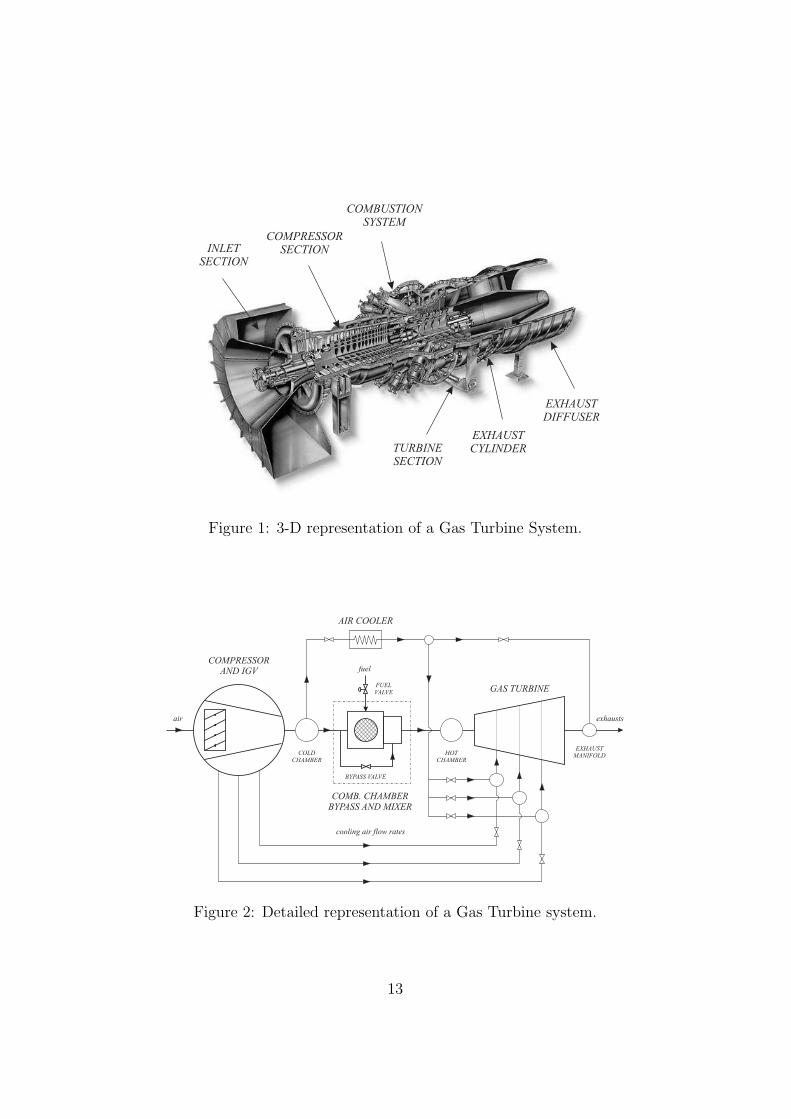
The three-dimensional section of an industrial GT system is shown in Figure1, while a schematic description is given in Figure 2. The main componentsof GT systems are the compressor, the combustion chamber (or burner) andthe gas turbine. Figure 2 also includes the Inlet Guide Valve (IGV), the fuelvalve, a mixer, located after the burner and associated to a bypass valve, theair cooler and the exhaust manifold (mixer), positioned after the gas turbine.From the figure, it is also possible to observe the air fluxes drained from dif-ferent stages of the gas turbine: they play the role of cooling flow rates ofthe turbine blades. Although GTs are complex systems, for the purposes ofthis Thesis, their modeling can be simplified as shown in Figure 3, where themain elements considered in the following are shown. Moreover, since theGTs are characterized by a faster dynamics with respect to the one of theHRSG systems, their model can be based on algebraic equations. In fact,their significant dynamic phenomena are mainly due to the system actuators:the IGV and the fuel feeding system. The IGV, regulating the inlet air flux,is characterized by a quite slow dynamics, with a time constant of about tenseconds. The fuel valve, instead, exhibits a faster response, with a settlingtime even lower than one second. Both these two devices may be modeled asfirst order systems, while the time delay of the masses flow through the GT

11

may be neglected.

The Compressor

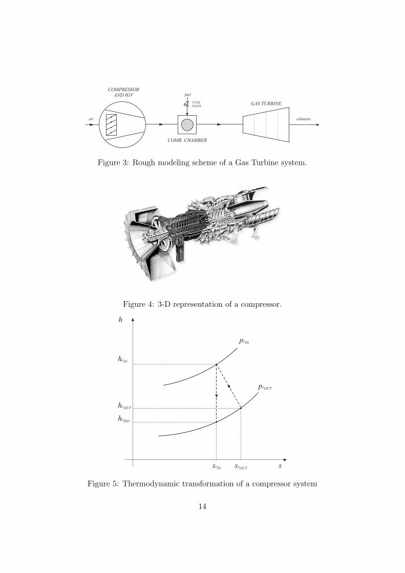
The compressor (see Figure 4) provides a high pressure air flow to the com-bustion chamber: the corresponding thermodynamic transformation is shownin Figure 5. With the same model it is possible to understand immediatelythe meaning of the compressor efficiency ηc, defined as:

ηc =haISO

− haIN

haOUT− haIN

(1)

where he definition of all the variables is reported in Table 1.

Input variablesqa air flow rate kg s−1

qa0 air flow rate at nominal road kg s−1

TaIN inlet air temperature K

Output variablesPc absorbed power WTaOUT

outlet air temperature K

Auxiliary variableshaIN inlet air enthalpy J kg−1

haOUToutlet air enthalphy J kg−1

haISOair isentropic enthalphy J kg−1

PaOUToutlet air pressure Pa

PaIN inlet air pressure Pa

Parameterscpc air equivalent specific heat J K−1 kg−1

ηc efficiency

Table 1: Compressor - variables and parameters.

To obtain a mathematical representation of the system, three generalphysical laws are here recalled:

12

INLET

SECTION

COMBUSTION

SYSTEM

COMPRESSOR

SECTION

TURBINE

SECTION

EXHAUST

CYLINDER

EXHAUST

DIFFUSER

Figure 1: 3-D representation of a Gas Turbine System.

COMPRESSORAND IGV

GAS TURBINE

AIR COOLER

COMB. CHAMBERBYPASS AND MIXER

COLDCHAMBER

HOTCHAMBER

EXHAUSTMANIFOLD

FUELVALVE

air exhausts

fuel

cooling air flow rates

BYPASS VALVE

Figure 2: Detailed representation of a Gas Turbine system.

13

GAS TURBINE

COMB. CHAMBER

air exhausts

COMPRESSORAND IGV

FUELVALVE

fuel

Figure 3: Rough modeling scheme of a Gas Turbine system.

Figure 4: 3-D representation of a compressor.

h

heIN

heISO

heOUT

peIN

peOUT

sseIN seOUT

Figure 5: Thermodynamic transformation of a compressor system

14

1. the definition of isentropic transformation

Tds = dh− 1

ρdp = 0 (2)

where T is the fluid temperature (K), s the specific entropy (JK−1kg−1),h is the specific enthalphy (Jkg−1), ρ is the mass density (kg m−3) andp is the pressure (Pa).

2. the definition of specific heat cp at constant pressure

cp =dh

dT(3)

3. the ideal gas lawp

ρ= αT (4)

where α is the thermodynamic constant

By proper substitutions, from equations (2), (3), and (4) it is possible toobtain the following equality:

cpdT =αT

pdp (5)

which can be integrated, thus obtaining, for the compressor, the followingrelation between temperatures and pressures (related to the isentropic trans-formation case):

TαISO

TαIN

=

(pαOUT

pαIN

) αcp

(6)

which can be assumed to be analogously valid for the enthalpies:

hαISO

hαIN

=

(pαOUT

pαIN

) αcp

(7)

By combining equation (7) with the compressor efficiency definition, it ispossible to obtain the expression of the outlet temperature and of the ental-phy (a simplification is used, the pressure ratio PR =

pαOUT

pαINis replaced with

the expression PR = PR0qαqα0

, where PR0 is defined as the nominal pressure

ratio, and its value coincides with PR at nominal load). The expressions are:

hαOUT= hαIN

(1 +

1

ηc

[(PR0

qαqα0

)ec

− 1

])(8)

15

TαOUT= TαIN

(1 +

1

ηc

[(PR0

qαqα0

)ec

− 1

])(9)

where ec =αcp.

With further simplifications and substitutions, it is possible to obtain thevalue of the mechanical power absorbed by the compressor:

Pc = qα1

ηc

[(PR0

qαqα0

)ec

− 1

]cpcTαIN

(10)

The Gas Turbine

The Gas Turbine (Figure 6) model relies on the same physical principlesand simplification already introduced for the compressor. Figure 7 shows thethermodynamic cycle of the turbine. Differently from the compressor case,where the mechanical power is needed to raise the air pressure, here the me-chanical power is obtained by the exhaust pressure drop. Table 2 reports thelist of all the model variables and parameters.

Figure 6: 3-D representation of Gas Turbine

The gas turbine efficiency is defined as

ηt =heIN

−heOUT

heIN−heISO

and, analogously to (6) and (7), one has:

TeISO

TeIN

=

(peOUT

peIN

) αcp

(11)

16

Input variablesqe exhaust flow rate kg s−1

qe0 exhaust flow rate at nominal road kg s−1

TeIN inlet exhaust temperature K

Output variablesPt generated mechanical power WTeOUT

outlet exhaust temperature K

Auxiliary variablesheIN inlet exhaust enthalpy J kg−1

heOUToutlet exhaust enthalphy J kg−1

heISOexhaust isentropic enthalphy J kg−1

PeOUToutlet exhaust pressure Pa

PeIN inlet exhaust pressure Pa

Parameterscpt exhaust equivalent specific heat J K−1 kg−1

ηt efficiency

Table 2: Gas Turbine - variables and parameters.

17

h

haOUT

haIN

haISO

s

paOUT

paIN

saIN saOUT

Figure 7: Thermodynamic transformation of a turbine system.

where TeIN = TeMIX, and

heISO

heIN

=

(peOUT

pαIN

) αcp

(12)

Differently from the compressor case, the value of the exponent et =αcp

can be identified according to the normal working conditions. Letting

peOUT

peIN=

pαOUT

pαIN

=1

PR(13)

and assuming that

peOUT

peIN=

1

PR0

qe0qe

(14)

it is possible to express the exhaust enthalphy and temperature at the turbineoutlet as

heOUT= heIN

(1− ηt

[1−

(1

PR0

qe0qe

)et])(15)

TeOUT= TeIN

(1− ηt

[1−

(1

PR0

qe0qe

)et])(16)

18

The expression of the power generated by the turbine is

Pt = qeηt

[1−

(1

PR0

qe0qe

)et]cptTeIN (17)

Combustion chamber, bypass and mixer

A very simplified formulation has been adopted both for the burner andthe subsequent air-exhausts mixer. The burner is described by the followingtwo equations

Tecc = Tacc + kfqfqacc

(18)

qecc = qacc + qf (19)

(see Tables 3 and 4 for a complete variables list), where qacc = qa − qaA.C.−

qaT.C., while the mixer is modeled as

TeMIX=

qaBY PASSTaBY PASS

+ qeccTecc

qaBY PASS+ qecc

(20)

qeMIX= qecc + qaBY PASS

(21)

where TaBY PASS= Tacc = TaOUT

. As previously mentioned, the bypass airflow rate value is assumed to vary proportionally with the compressor inletair flow rate:

qaBY PASS= kaBY PASS

qa

1.1.2 The Heat Recovery Steam Generator

The HRSG represents the more complex subsystem of a CCPP. Its modularnature suggests to perform an independent model of the elementary (dy-namic) blocks composing the boiler (heat exchangers, evaporators and steamturbine stages), in order to subsequently obtain a complete model (and sim-ulator) of the steam generator by assembling them according to the planttopology. An algebraic solution has been adopted for both the steam fluiddynamics and the water hydrodynamics (except for the regulating actuators,valves and pumps). This choice takes also advantage of the separate model-ing of the thermodynamic and fluid dynamic phenomena: the link between

19

Input variablesqacc inlet air flow rate kg s−1

qf air flow rate at nominal road kg s−1

Tacc inlet air temperature K

Output variablesqecc outlet exhaust flow rate kg s−1

TaOUToutlet exhaust temperature K

Parameterskf fuel equivalent burning power K

Table 3: Combustion chamber - variables and parameters.

Input variablesqaBY PASS

bypass air flow rate kg s−1

qecc comb. chamber outlet exhaust flow rate kg s−1

TaBY PASSinlet air temperature K

qecc comb. chamber outlet exhaust temperature K

Output variablesqeMIX

outlet exhaust flow rate kg s−1

TeOUToutlet exhaust temperature K

ParameterskaBY PASS

bypass air flow rate ratio K

Table 4: Mixer and bypass - variables and parameters.

20

DIFFUSER

DRUM BOILERS

CHIMNEY

Figure 8: The Heat Recovery Steam Generator

them is represented by the drum boilers pressure. A three-dimensional rep-resentation of a HRSG is proposed in Figure 8.

Heat exchangers

A schematic representation of a heat exchanger is usually adopted: a rec-tilinear metal pipeline with an outer exhausts side and an inner water (inthe economizers case) or steam (for superheaters and reheaters). Throughthe metal, the heat exchange between the two fluxes occurs: commonly, thecountercurrent solution (i.e. with the two fluxes flowing in opposite direc-tions) is preferred, by virtue of its greater efficiency, while the co-currentconfiguration may be adopted, for example, when it is necessary to protectthe metal from too high thermal stresses.In the plant considered in this Thesis, a countercurrent solution has beenused. The following analysis, describing the adopted simplified heat ex-changer model, refers to the exhausts-to-steam countercurrent case: withminor modifications the same modeling approach can be used also for theeconomizers.Countercurrent exhaust-to-steam heat exchangerAs regards the fluid dynamics, the pressure drop through the exchanger has

21

not been taken into account: a unique value of the fluid pressure, correspond-ing to the inlet section and provided by the solution of the fluid dynamicsystem (discussed in Section 3.9), has been considered and counted amongthe model input variables.The main simplifying assumptions adopted in the thermodynamic model aresubsequently summarized:

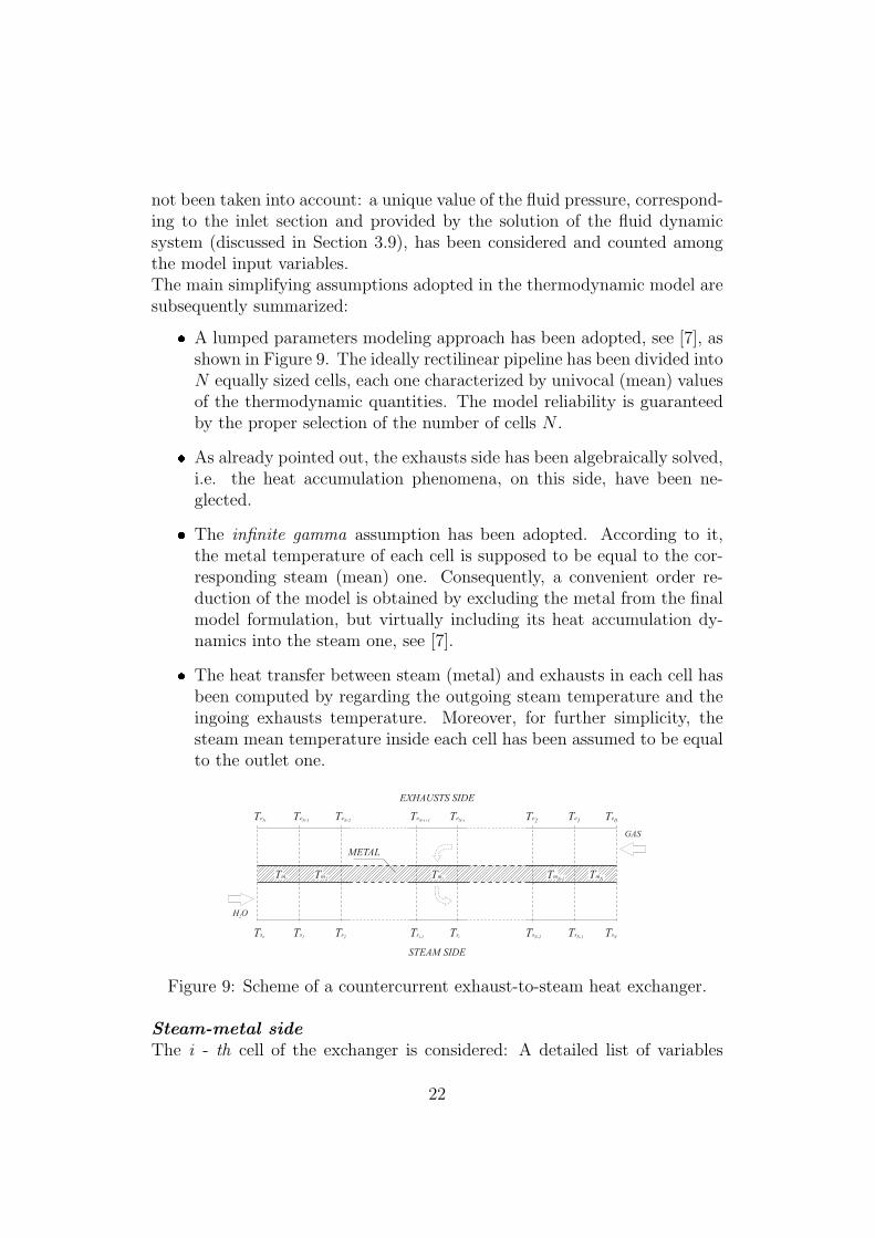
� A lumped parameters modeling approach has been adopted, see [7], asshown in Figure 9. The ideally rectilinear pipeline has been divided intoN equally sized cells, each one characterized by univocal (mean) valuesof the thermodynamic quantities. The model reliability is guaranteedby the proper selection of the number of cells N .

� As already pointed out, the exhausts side has been algebraically solved,i.e. the heat accumulation phenomena, on this side, have been ne-glected.

� The infinite gamma assumption has been adopted. According to it,the metal temperature of each cell is supposed to be equal to the cor-responding steam (mean) one. Consequently, a convenient order re-duction of the model is obtained by excluding the metal from the finalmodel formulation, but virtually including its heat accumulation dy-namics into the steam one, see [7].

� The heat transfer between steam (metal) and exhausts in each cell hasbeen computed by regarding the outgoing steam temperature and theingoing exhausts temperature. Moreover, for further simplicity, thesteam mean temperature inside each cell has been assumed to be equalto the outlet one.

TeN

TeN-1

TeN-2

TeN-i+1

TeN-i

Te2

Te1

Te0

Ts0

Ts1

Ts2

Tsi-1

Tsi

TsN-2

TsN-1

TsN

EXHAUSTS SIDE

STEAM SIDE

H O2

GAS

Tm1

Tm2

Tmi

TmN-1

TmN

METAL

Figure 9: Scheme of a countercurrent exhaust-to-steam heat exchanger.

Steam-metal sideThe i - th cell of the exchanger is considered: A detailed list of variables

22

and parameters is reported in Tables 5 and 6. The heat accumulation insidesteam and metal is described by the following energy balances, respectively

cpsmsidT si

dt= qscps(Tsi−1

− Tsi) + γISIi(Tmi− T si)

cmmmi

dTmi

dt= γOSOi

(TeN−1− Tmi

)− γISIi(Tmi− T si)

(22)

for i = 1, . . . , N . By dividing both the equations in (22) by qscps and definingthe constants:

τsi =cpsmsi

qscps=

msi

qs(23)

andτmi

=cmmmi

qscps(24)

which represent the two time constants associated to the steam and metalheat storing, respectively (note that τmi

>> τsi), equations (22) can berewritten as follows

τsidT si

dt= (Tsi−1

− Tsi) +γISIi

qscps(Tmi

− T si)

τmi

dTmi

dt=

γOSOi

qscps(TeN−1

− Tmi)− γISIi

qscps(Tmi

− T si)

(25)

The infinite gamma assumption is now introduced: the heat exchangecoefficient γI between metal and steam is assumed to be virtually infinite.As a consequence, the metal and the steam mean temperatures inside a cellturn out to be identical, as it is easy to prove by rearranging the first equationin (22) and by dividing both its sides by γISIi

Tmi− T si =

1γISIi

(cpsmsi

dT si

dt− qscps(Tsi−1

− Tsi))

limγI→∞ Tmi− T si = 0 ⇒ Tmi

= T si

(26)

Once stated that Tmi= T si , it is possible to describe the cell thermodynamics

by means of a single equation, obtained by adding equations (25) together

(τsi + τmi)dT si

dt= (Tsi−1

− Tsi) +γOSOi

qscps(TeN−1

− T si) (27)

Exhaust sideFor the exhausts side, it is assumed that no heat accumulation occurs (noenergy variation characterizes the exhausts inside the cell volume), this allowsfor a simple algebraic modeling of the gases energy balance, i.e.

23

Input variablespsIN inlet steam pressure Paqe exhaust flow rate kg s−1

qs steam flow rate kg s−1

TeIN = Te0 inlet exhaust temperature KTsIN = Ts0 inlet steam temperature K

State variablesTsi i - th cell outlet steam temperature KAlgebric variablesTeN−i

i - th cell outlet exhaust temperature KOutput variablesTeOUT

= TeN outlet exhaust temperature KTsOUT

= TsN outlet steam temperature K

Auxiliary VariableshsIN inlet steam enthalphy J kg s−1

hsOUToutlet steam enthalphy J kg s−1

Eei i - th cell exhaust stored energy Jρsi i - th cell steam mass density kg m−3

Tmii - th cell metal mean temperature K

T si i - th cell steam mean temperature K

Table 5: Heat exchanger model - variables.

24

cm metal heat capacity J K−1 kg−1

cpe exhaust specific heat J K−1 kg−1

cps steam specific heat J K−1 kg−1

γI metal-steam (inner side) heat exch. coeff. W m−2 K−1

γO exhaust-metal (outer side) heat exch. coeff. W m−2 K−1

Γe exhaust-metal empiric heat exch. coeff. W K−1 kg−0.6 s−0.6

Γs steam-metal empiric heat exch. coeff. W K−1 kg−0.6 s−0.6

i cell indexmmi

i - th cell metal mass Kmsi i - th cell steam mass KN number of cellSI exchanger inner surface m2

SIi i - th cell inner surface m2

SOii - th cell outer surface m2

Vsi i - th cell steam volume m3

Table 6: Heat exchanger model - parameters.

dEei

dt= qecpe(TeN−i

− TeN−i+1)− γOSOi

(TeN−1− Tmi

) = 0 (28)

By replacing Tmiwith Tsi in (28), in accordance with (26) and the as-

sumption of equality between T si = Tsi , and by rearranging it in order tomake TeN−i+1

explicit, one obtains

TeN−i+1= TeN−i

− γOSOi

qscps(TeN−1

− Tsi) (29)

According to a commonly adopted empirical law, the quantity γOSOihas to

be replaced with the term Γeq0.6e , so as to introduce the proper dependance

of the heat transfer on the exhausts flow rate.Then, it is possible to write the final equations (one algebraic and one

dynamic) for the thermodynamic behavior of each cell:dTsi

dt= 1

τsi+τmi

[(Tsi−1

− Tsi) +Γeq0.6e

qscps(TeN−i

− Tsi)]

TeN−i+1= TeN−i

− Γeq0.6e

qecpe(TeN−1

− Tsi)

(30)

25

Economizers (exhaust-to-water heat exchangers)

As already pointed out, the proposed model can be applied also to the econ-omizers provided that the following changes are made:

1. the water mass density ρω is assumed to be constant (ρω = 103 kg m−3),thus simplifying the computation of the time constants;

2. the introduction of a pressure-varying cpw coefficient is unnecessary.

As a consequence of these changes, the value of the inlet water pressure isnot needed.

The Drum Boiler

A detailed scheme of the drum boiler (or evaporator) is provided in Figure10. Its main components are:

� the drum, a cylindrical cavity containing saturated steam and water;

� the downcomers, the descending pipelines conveying the water from thedrum to the re-circulation pump;

� the risers, i.e. the ascending pipelines which allow the thermal exchangebetween the hot exhausts and the steam-water fluid, thus giving riseto the steam production.

Concerning the process dynamics, the drum boiler behavior is describedthrough the steam-water pressure and the water level inside the drum.

The steam production, is strictly correlated with the pressure dynamics.Based on mass and energy balances, the drum boiler model is the mostcomplex component of the HRSG: its modeling required significant effortsto capture the true process nonlinearities. The reasons of such a complexitymay be briefly summarized.

1. The strong coupling between the thermodynamic and the fluid dynamicprocesses. Suffices here to remember that all the thermodynamic prop-erties of the saturated steam and water are functions of the drum boilerpressure. Moreover, by virtue of the interaction between the evaporatorand the steam turbine, the outgoing steam flow rate directly dependson the pressure level established inside the cavity (and turns out to beapproximatively proportional to the generated mechanical load).

26

2. The presence of both (saturated) steam and water (in the risers zone,in particular).

DRUM

DOWNCOMERS

RISERS

RECIRCULATION PUMP

outlet steamflow rate

outlet waterflow rate

inlet waterflow rate

hot exhaustsflow rate

RECIRCULATIONCIRCUIT

steamproduction Qe

qsr

qwr

qd

y

qe

qs

water level

steam

water qwINqwOUT

Figure 10: Evaporator scheme

A very complete model of the drum boiler has been developed in [6], wherenatural circulation drum boilers, characterized by strong nonlinearities andan accentuated “shrink and swell dynamics�have been considered. In thisThesis, the model described in [4] has been adopted. It is a 3rd−order modelwhere the distribution of steam and water inside the drum has been treatedin a simpler way than in [6]. For conciseness, the model is not reported here,and the interested reader is referred to [4] for details.

27

1.1.3 Steam turbine stage

As for the gas turbine, an algebraic model turns out to be suitable also forthe steam turbine stages. Actually, the system under inspection includesboth the steam turbine and the inlet (or “throttle”) valve: the utilizationof this latter depends on the adopted plant management strategy. Usually,the steam turbine valves are kept completely open (this working mode iscommonly defined as sliding pressure), in order to guarantee the highestplant efficiency. Alternatively, it may be possible to adopt a different policyof plant regulation by keeping the throttle valves slightly closed at low loads,while opening them wide to exploit the so called steam supply when a loadrequest occurs 10 . The system including the steam turbine and its throttlevalve (corresponding to a pressure stage of the whole steam turbine) will behereafter denoted as “Steam Turbine System”(STS). Its role is to generatethe mechanical load by interacting with the steam generator. Figure 11offers a schematic diagram of the STS, while Table 7 provides a list of all itsvariables and parameters.

STEAM TURBINE

throttle valveSH / RH

nozzle

wheel

ps

turbine axle

discharge

psINpsnozzle

psOUT

qs P

Figure 11: Diagram of the STS

The proposed algebraic model consists of three equations.

1. The first one deals with the steam flow rate. As previously remarked,

28

Input variablespsIN inlet steam pressure PapsOUT

outlet steam pressure PaTsIN inlet steam temperature Kϑ throttle valve opening

Output variablesP generated mechanical power Wqs steam flow rate kg s−1

TsOUToutlet steam rate K

Auxiliary VariableshsIN inlet steam specific enthalphy J kg s−1

hsISOsteam isentropic specific enthalphy J kg s−1

hsOUToutlet steam specific enthalphy J kg s−1

psnozzlenozzle inlet steam pressure Pa

ρsIN inlet steam mass density kg m−3

TsISOi - th cell steam mean temperature K

ParametersAn nozzle section m2

Av throttle valve section m2

cp mean steam specific heat J K−1 kg−1

ηt turbine efficiency J kg s−1

Table 7: Steam Turbine System - variables and parameters

29

the steam turbine interacts with the evaporator. This latter imposesthe upstream pressure level on the basis of both the heat power providedby the hot exhausts to the risers and the (required) outlet steam flux.A pressure drop occurs through the superheaters chain: on the basisof the resulting inlet pressure, the STS determines the steam flow rate,which needs to be provided by the steam generator;

2. The second one regards the generated mechanical load;

3. The third one allows the computation of the outlet steam temperature.

As for the heat exchangers, a temperature-based model has been adopted.This choice affects the second and particularly the third model equation.

Steam flow rate

As proposed in [13] in detail, the steam flow rate through the throttle valveis described by the equation:

qs = kvAv√ρsINpsINχ

(psnozzle

psIN

)(31)

where χ() is a universal function, which applies to all valves, while kv is aconstant parameter. The superheated steam may be considered as a perfectgas, thus allowing to assume that:

ρsIN =psINRTsIN

where R is the thermodynamic constant of the steam-gas. The equation 31became:

qs = kvAvpsIN

√1

RTsIN

χ

(psnozzle

psIN

)(32)

The same relation is valid for the turbine nozzle too, i.e.

qs = knAnpsnozzle

√1

RTsnozzle

χ

(psOUT

psnozzle

)(33)

where kn is the constant parameter (as shown in Figure 11, a simplifiedscheme of the steam turbine including a single internal stage has been as-sumed as the reference). As for the throttle valve, it is possible to assumethat Tsnozzle

≈ TsIN , while, in accordance with the design features of the

30

steam turbines, the pressures ratio psOUT/psnozzle

is constant with the steamflow rate qs. So, by comparing (32) with (33), one obtains

psINpsnozzle

χ

(psnozzle

psIN

)(34)

Equation (34) proves that the quantity psnozzle/psIN can be regarded as a

function of the only inlet section Av , regulated through the correspondingthrottle valve, i.e.

psnozzle/psIN = ft(Av)

Thanks to the most common design practice, which aims at an easier andfaster turbine control, the function ft(Av) exhibits an almost linear behaviorwith the valve control signal ϑ

ft(Av) ≈ kϑϑ

where kϑ is a constant gain. It follows that

qs = ktϑpsIN

√1

TsIN

(35)

The coefficient kt can be easily tuned on the basis of the nominal operatingpoint.

Generated mechanical power

As for the gas turbine, the generated power is given by:

P = qs(hsIN − hsOUT) (36)

To match the adopted temperature-based modeling of thermodynamics, equa-tion (36) needs to be modified as follows:

P = qscp(TsIN − TsOUT) (37)

where the equivalent specific heat cp may be identified on the basis of therated working conditions.

Outlet steam temperature

From a thermodynamic point of view, each steam turbine stage is analogous

31

to the gas turbine. Therefore, the outlet exhausts enthalpy and tempera-ture equations, (15) and (16) respectively, may be regarded as a reference.However, in this case, it is not required to replace the outlet-inlet pressureratio with an alternative function of the flow rate. Rather, it is necessary toconsider the difference between the behavior of the superheated steam anda perfect gas (like the hot exhausts, in the gas turbine), which claims tocarefully inspect the reliability of a temperature-based model formulation.By recalling the efficiency definition, here referred to the steam case:

hsIN−hsOUT

hsIN−hsISO

the following expression of the steam enthalphy at the turbine outlet is ob-tained:

hsOUT= hsIN

(1− ηt

[1−

(psOUT

psIN

)e])(38)

where the exponent e = α/cp may be computed on the basis of the selectedworking point

e =log

(hsISO

hsIN

)log

(psOUT

psIN

) (39)

Unlike the gas turbine, there are two different specific heat for input steamand for output steam. Because of this, a coefficient kiso is defined:

kiso =TsISO

TsIN

hsIN

hsISO

Then it’s possible to derive the required expression of the outlet steam tem-perature:

TsOUT= TsIN

(1− cpOUT

cpISO

ηt

[1− kiso

(psOUT

psIN

)e])(40)

1.1.4 Mixers and attemperators

The temperature-based modeling of a single-fluid (water or steam) mixer is aquite simple task, according to mass balances and the adiabatic mixing law.The basic configuration is shown in Figure 12: it roughly reproduces boththe two steam-mixers situated after the HP and IP steam turbines outlet andthe water-mixer located before the ECO-LP. This latter is equipped with arecirculation circuit, intended for the regulation of the inlet water tempera-ture: the aim is to avoid too low temperatures of the exhausts leaving theHRSG, which cause corrosive condensation in the colder part of the boilerand pollutants production. A list of the system variables is provided in Table

32

8.

According to the mass balance, one has

qs,wOUT= qs,wIN1

+ qs,wIN2(41)

while the adiabatic mixing law states that

hs,wOUT=

qs,wIN1hs,wIN1

+ qs,wIN2hs,wIN2

qs,wIN1+ qs,wIN2

(42)

which may be rewritten as

cpOUTTs,wOUT

=qs,wIN1

cpIN1Ts,wIN1

+qs,wIN2cpIN2

Ts,wIN2

qs,wIN1+qs,wIN2

By assuming

cpOUT≈ cpIN1

≈ cpIN2

as it is reasonable, one obtains

Ts,wOUT=

qs,wIN1Ts,wIN1

+ qs,wIN2Ts,wIN2

qs,wIN1+ qs,wIN2

(43)

MIXER

1st steam / waterinlet flow rate

2nd steam / waterinlet flow rate

steam / wateroutlet flow rate

Figure 12: Basic configuration of a mixer

For the attemperators, which add an adjustable cold water flow rate tothe superheated steam flux to reduce the steam temperature, the assumptionabout the approximation of specific heat (cpOUT

≈ cpIN1≈ cpIN2

) is not valid.

33

First inlet steam/water fluxcpIN1

specific heat J kg−1 s−1

hs,wIN1specific entalpy J kg−1

qs,wIN1flow rate kg s−1

Ts,wIN1temperature K

Second inlet steam/water fluxcpIN2


hs,wIN2specific entalpy J kg−1

qs,wIN2flow rate kg s−1

Ts,wIN2temperature K

Outlet steam/water fluxcpOUT


hs,wOUTspecific entalpy J kg−1

qs,wOUTflow rate kg s−1

Ts,wOUTtemperature K

Table 8: Mixer - variables and parameters

34

A possible way to perform a temperature-based modeling of the SH and RHattemperators consists of a proper rearrangement of (42), in accordance witha suitable local linearization of the enthalpy-temperature relation.Actually, such a linearization is required only for the steam fluid. In fact,the value of enthalpy of the desuperheating water, provided by the LP drumboiler, is available through the adopted evaporator model, which relies onproperly identified polynomial functions of the thermodynamic propertiesof the saturated steam and water. It is convenient to remember that theinjection of a small cold water flow rate into the superheated steam fluximplies only a cooling action of the steam (no state modification occurs).A linearization of the inlet steamenthalpy is adopted

hsIN (TsIN ) = hs0 + cp0TsIN (44)

All the model variables are summarized in Table 9. The outlet steam enthalpyis given by the adiabatic mixing law (42)

hsOUT=

qsIN hsIN(TsIN

)+qwINhwIN

qsIN+qwIN

Finally, recalling (44), the outlet steam temperature may be computed as

TsOUT=

1

cp0(hsOUT

− hs0) (45)

while the outlet steam flow rate is obtained from the mass balance

qsOUT= qsIN + qwIN

By means of the Steam Tables it is possible to perform the required lineariza-tion, which allows the proper tuning of the quantities cp0 and hs0 , on thebasis of the nominal working conditions.

1.1.5 Model of the thermo-mechanical stresses in the turbine ro-tor

In the start-up phase of a CCPP, one of the main requirements is to limitthe thermo-mechanical stresses of the turbine. In fact, the overall life of theplant mainly depends of the stress level reached in the start-up and shut-down phases, rather than in the total run time. For this reason, a reliablemodel of the stress of of paramount importance for the design of the start-up,i.e. of the main object of this work. In the following, the model developedin [9] and subsequently used in [12], is briefly summarized.In our calculations leading to the final model, it is possible to assume a one

35

Inlet superheated steamhsIN specific entalpy J kg−1

qsIN flow rate kg s−1

TsIN temperature K

Inlet subcooled waterhwIN

specific entalpy J kg−1

qwINflow rate kg s−1

Outlet steam/water fluxhsOUT

specific entalpy J kg−1

qsOUTflow rate kg s−1

TsOUTtemperature K

Table 9: Attemperators - variables

dimensional radial model of the component we are interested in. The geom-etry of this desired component is a smooth cylindrical cavity and we assumethat the total length is much larger than the diameter. In this context wecan assume an axial-symmetrical temperature distribution. The assumptionof axial-symmetric conditions simplifies the modeling and the solution of thenecessary equations. An approximation of the one-dimensional radial tem-perature heat transfer can be expressed with cylindrical coordinates in thefollowing form:

ρcpk

δT

δt=

1

r

δ

δr

(rδT

δr

)(46)

where ρ and cp represent the density and the specific thermal conductivityof the material used in the component. T is the temperature of this materialand r and t respectively represent the radial coordinate and time. For thenumerical solution od this equation we may use spatial discretization involv-ing the finite difference method. The right hand of equation (46) is hencediscretized and rewritten as:

1

ri

[(r δTδr

)i+1/2

−(r δTδr

)i−1/2

]ri+1/2 − ri−1/2

=1

ri(ri+1/2 − ri−1/2

) (ri+1/2Ti+1 − Ti

ri+1 − ri− ri−1/2

Ti − Ti−1

ri − ri−1

)(47)

36

The left-hand-side of (46) can be set equal to the equation (47), to obtainthe results shown in (48).

ρcpk

δT

δt= AiTi−1 +BiTi + CiTi+1 (48)

where Ai and Ci are the coefficients:

Ai =ri−1/2

ri(ri−ri−1)(ri+1/2−ri−1/2)

Bi = −(Ai + Ci)Ci =

ri+1/2

ri(ri−ri−1)(ri+1/2−ri−1/2)

Then, the general conditions for the stress can be rewritten as

Ti = Tint

TNr = Text

ϕint = −k T2−T1

r2−r1

ϕext = −kTNr−TNr−1

rNr−rNr−1

The Fourier discretized component of the model of the internal and externalstresses can be written as in equation (49)

σT,r = 0σT,θ =αE

1− v(Tm − Tint/ext)σT,z =

αE

1− v(Tm − Tint/ext) (49)

where α is the dilation constant, E is the Young Modulo, v is the Poissonratio relatively to the material used in the component and Tm , Tint and Text

are the medium, internal and external surface temperatures of the material.The mechanical stresses in the rotor can be written as in equation (50)

σc,θ =3 + v

4ρω2

(r2int/ext −

1− v

3 + vrint/ext

)(50)

The external surface of the rotor is the part of the rotor that is in directcontact with the hot gases.

37

1.2 Plant data

In [4] and [8] CCPP models have been developed starting from the elemen-tary models of the subsystems composing a CCPP, some of which have beendescribed in the previous sections. Both in [4] and in [8], HRSG subsystemswith three pressure stages have been developed and simulated in differentenvironments (Matlab/Simulink in [4] and Modelica in [8]). These modelsand simulators, although very accurate, are not suitable for the developmentof innovative strategies for the start-up phase. In particular, the Simulinkmodel described in [4] is computationally very demanding and not suited torepresent the significant dynamic phenomena inside the CCPP at very lowloads. On the contrary, the Modelica model described in [8], is more general,since it can completely describe the overall operating range of the CCPP.However, the model is even too complex for the project of the start-up pro-cedure. For these reasons, in the framework of the EU project “Hierarchicaland Distributed Control of Large Scale Systems”, starting from the Model-ica model first introduced in [9], [8] and already used in [12], SUPELEC hasdeveloped a simpler CCPP model, composed by a gas turbine (GT) and onlyone pressure stage in the HRSG, see [15].

Gas TurbineThe Gas Turbine system, which does not represent a limiting factor for thestart-up since the HRSG dynamics is much slower than the GT one, is char-acterized by the following nominal data:

� maximal power of 235 [MW];

� nominal flue gas flow rate of 585.6 [kg/s];

� nominal fuel flow rate of 12.1 [kg/s].

Heat Recovery Steam GeneratorThe considered HRSG has a single pressure circuit (high pressure) with:

� nominal HP steam flow rate of 70.6 [kg/s];

� nominal HP steam pressure of 129.6 [bar].

The HP circuit has the following components:

� economizer;

� steam drum;

� evaporator;

38

� superheater.

Steam LinesThe system of pipes connecting the HRSG, the ST and the condenser, hasa length of 130 [m] and is provided with an evacuation system to eliminatethe condensates.

Input and output variablesSince the objective of this project is to design a control system for the plant,in particular with reference to the start-up phase, it is mandatory to havethe possibility to monitor the main input and output variables. From themodel developed by SUPELEC, it is possible to have full knowledge of thefollowing variables.Inputs:

� GT Load: load of gas turbine;

� Feed Drum: feedwater flow rate for the HRSG circuit;

� Feed DSH: water flow that feeds the desuperheater;

� Bypass ST : position of the bypass valve;

� V alve ST : position of the turbine admission valve;

� BreakerClosed: generator grid breaker of the steam turbine.

Outputs:

� GT Power: power produced by the gas turbine;

� GT Fuel: fuel flow in the gas turbine;

� Drum Level: drum level of the HRSG;

� T SH: temperature of steam in the superheater;

� Steam Press: steam pressure;

� Header Stress: thermodynamical stress of the header;

� T SL: temperature of steam in the steam line;

� ST Power: power produced by the steam turbine;

� ST Frequency: frequency of the steam turbine;

39

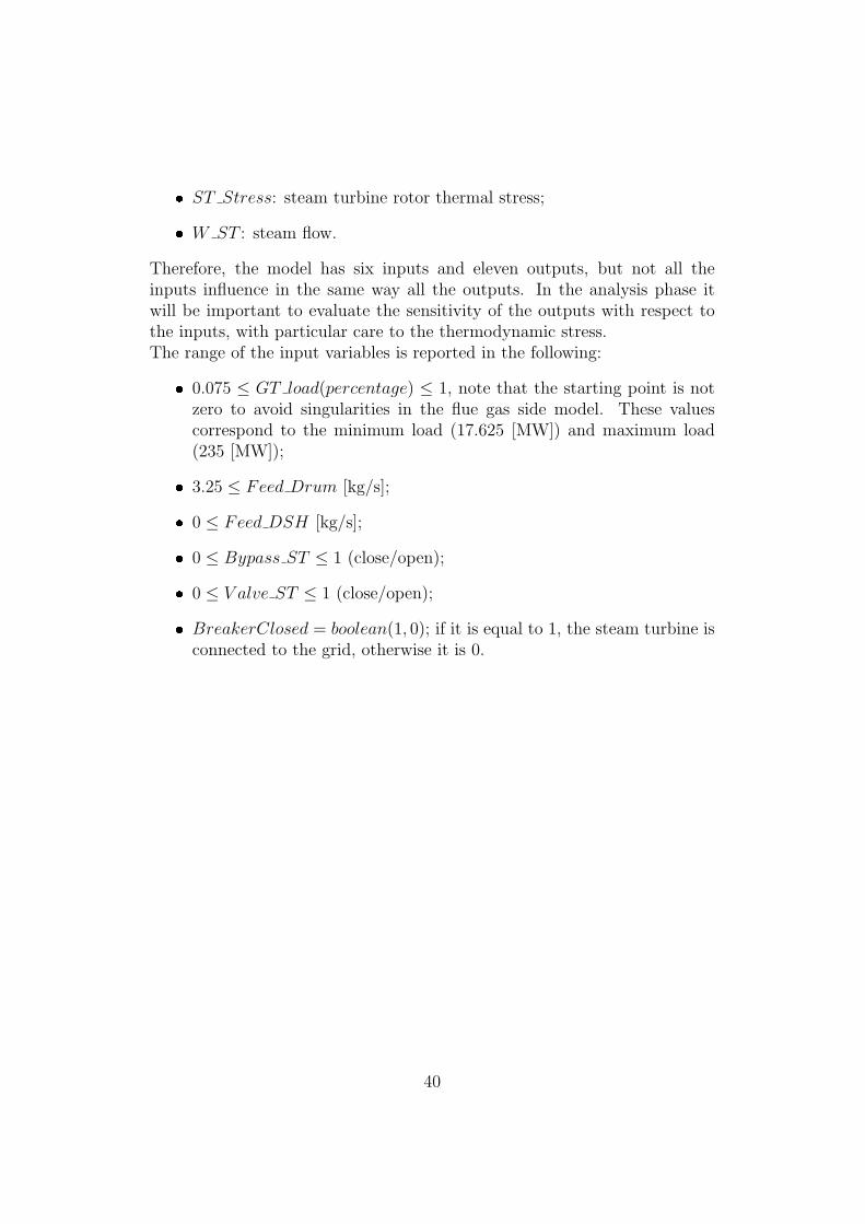
� ST Stress: steam turbine rotor thermal stress;

� W ST : steam flow.

Therefore, the model has six inputs and eleven outputs, but not all theinputs influence in the same way all the outputs. In the analysis phase itwill be important to evaluate the sensitivity of the outputs with respect tothe inputs, with particular care to the thermodynamic stress.The range of the input variables is reported in the following:

� 0.075 ≤ GT load(percentage) ≤ 1, note that the starting point is notzero to avoid singularities in the flue gas side model. These valuescorrespond to the minimum load (17.625 [MW]) and maximum load(235 [MW]);

� 3.25 ≤ Feed Drum [kg/s];

� 0 ≤ Feed DSH [kg/s];

� 0 ≤ Bypass ST ≤ 1 (close/open);

� 0 ≤ V alve ST ≤ 1 (close/open);

� BreakerClosed = boolean(1, 0); if it is equal to 1, the steam turbine isconnected to the grid, otherwise it is 0.

40

1.3 Modelica Model

In order to develop an efficient simulator of the CCPP, the dynamic modelpreviously described has been implemented in Modelica, a powerful objectoriented language used for modeling large, complex, and heterogeneous phys-ical systems.The most important features of Modelica are:

� Object-oriented modeling. This feature allows one to create physicalmodel components, employed to support hierarchical structuring, reuse,and evolution of complex models from several different domains.

� Acausal modeling. Modelica is based on equations instead of assign-ment statements. Direct use of equation gives a better reuse of modelcomponents, since the components adapt to the data flow context inwhich they are used.

� Physical modeling. The model components can correspond to realphysical objects. The structure of the model is more natural sinceit implements the traditional concept based on block-oriented models.

The use of the modeling language Modelica in model based process controlapplications has many advantages. In fact, Modelica allows one to describea large class of models (linear, nonlinear, hybrid etc.) and many efficientsoftware tools [2], [1], [3] are available. On the other hand, there are fewtools supporting Modelica for static and dynamic optimization, see e.g. [10]for a remarkable exception.

The CCPP model has been developed with the Dymola tool, see [3], anduses the components from the ThermoPower library, see [14], an open-sourcelibrary for modeling thermal power plants at the system level, as well as tosupport the design and validation of control systems. The library has beendeveloped according to following principles:

1. the models are derived from first principle equations or from knownempirical correlations;

2. the model interface is totally independent of the modeling assumptionadopted for each model, to achieve full modularity;

3. the level of detail of the models is flexible;

4. the inheritance mechanism is used with limitation, to maximize thecode readability and modifiability.

41

The plant model has the following features:

� can represent the whole start-up sequence, [15];

� includes a model of the thermal stress in some critical components,which is the most limiting factor for the start-up time, [15];

� neglects phenomena and components which are not critical for the start-up sequence, in order to keep the complexity of the model at a reason-able level.

The highest level of the CCPP Modelica simulator is shown in Figure13; all the components (exploding the main model of Figure 13) are shownin Figure 14. In this scheme, it is possible to see the blocks correspondingto the gas turbine system, the HRSG, the steam line, the sink (substitutingthe intermediate pressure stage) and the steam turbine. The input/outputblocks are standard Modelica blocks. A higher level of detail is presentedin [9]

42

Figure 13: Modelica model of CCPP

43

Figure 14: Dymola components

44

2 Chapter 2: Identification of a simplified

model

The CCPP model described in the previous chapter is highly complex andcharacterized by strongly nonlinear dynamics. Moreover, as already noted,the Modelica environment is not yet equipped with adequate ancillary toolsfor control design and optimization. For these reasons, in this chapter atten-tion is paid to the identification of a simpler model, to be implemented in theMatlab/Simulink environment, which will be subsequently used to determinethe plant start-up procedure. The Modelica simulator will then be used as areference model to produce the data for identification and validation.

2.1 Identification approach: interpolation of linear mod-els

The identification of nonlinear process models is a challenging task: non-linearities, changes in the directionality of the gain, discontinuities are phe-nomena typical of the CCPP behavior which is very difficult to capture withstandard estimation procedures. Many different solutions have been proposedin the literature, for example nonlinear structures based on Neural Networks(NN) have been extensively studied. However, the models so obtained aretypically black-box and do not guarantee a high level of transparency, so thatthe main dynamic phenomena are often hidden to the user. Moreover, theidentification phase often relies on emphirical considerations, for instance inthe definition of the model structure (number of neurons and hidden layersin NN, number and type of regressors in polynomial models).For these reasons, the approach adopted in the following is different andquite easy to understand for anyone familiar with the use of linear (or lin-earized) models. The idea is simple and requires to decompose the nonlinearidentification problem into a number of linear identifications using processinformation. As a matter of fact, a number of plant operating points is se-lected, possibly covering the overall operating range of the system. Then, atany operating point, a local linear model is estimated by means of standardidentification procedures (based on the Least Squares method, for example).Finally, the overall identified plant model is obtained by suitably interpolat-ing at any operating point the local linear models through the use of weightsspecified by properly chosen membership functions. Indeed, these weightsdefine the validity, at any operating point, of the locally estimated transferfunctions. This method, although pretty empirical, has already been suc-cessfully used in a number of applications, see [11], [5].

45

In the case of the CCPP system, the model to be identified has three inputs:GT Load, V alve ST and Feed DSH (recall that the Feed Drum is con-trolled with a local regulator to avoid problems of an excessive increase/de-crease of the level inside the drum boiler, while the Bypass ST and theBreakerClosed are constant with the bypass valve totally open and the loadgrid connected). The gas turbine load is used as the scheduling variable, i.e.as the variable specifying the current operating condition. Therefore, thelocal linear models are identified at different steady-state conditions corre-sponding to a fixed value of the GT Load. Interpolation of the local linearmodels is then performed depending on the value of the load. This choiceis somehow obvious, since this variable governs the start-up and shut-downphases of the plant.

At each operating point, a local perturbation with the shape of a squaresignal has been imposed at any input of the Modelica model to generate thedata subsequently used to identify with the Matlab Identification Toolbox alocal linear model.Then, letting y the (output) variable to be identified, y its nominal valuein the considered operating point, ui the nominal value of the i − th input(i = 1, 2, 3), µi the imposed perturbation, δi the contribution of the i − thinput to the output and Gi(s) the local (identified) linear transfer functionrelating the i − th input to the δi component, the scheme of the overallidentified local model for the generic output y is reported in Figure 15.

Figure 15: Scheme of the identified model at generic operating point.

Once a local linear model has been identified for any output variable ofinterest at any of the selected N operating points, a suitable interpolationprocedure must be defined. To this regard, an approach based on the use ofmembership functions has been adopted. The membership functions mustbe selected so that for any value of the scheduling variable (the GT Load)the weight associated to the model estimated at the nearest operating point

46

provides a bigger contribution than the others. The final identified modelturns out to have the structure reported in Figure 16.

An example of the adopted membership functions is reported in Figure17: it is important to note that in every point the sum of the membershipfunctions is equal to one. Every function is associated to one of the oper-ating points where local models have been identified, however, the slope ofthe membership functions must be properly tuned to obtain an overall modelwhose validity covers the complete operating range of the CCPP. The defini-tion of the membership functions for each output variable requires a specifictuning, and the definition of their parameters can be time consuming. How-ever, in future developments, the tuning of the membership functions couldbe automatized through an optimization procedure.

Figure 16: Interpolation with membership functions.

In conclusion, the identification algorithm for the CCPP can be summa-rized as follows:

1. determine the operating points where to perform local identifications;

2. simulate the Dymola model by forcing small perturbations around anyoperating point and store the corresponding transient to be used foridentification;

3. identify the local linear models with the Matlab Identification Toolbox ;

47

2000 2200 2400 2600 2800 3000 32000

0.1

0.2

0.3

0.4

0.5

0.6

0.7

0.8

0.9

1

Figure 17: Example of membership functions.

4. select the membership functions and build the interpolation schemewith Matlab Simulink.

2.2 Selection of the operating points for identification

The choice of the operating points where to perform the identification is atradeoff between physical properties of the plant and interpolation require-ments. In fact, some points have particular physical relevance, but can notbe sufficient to describe the dynamics of the plant. Initially, the followingpoints were chosen:

� 100% of GT Load, defines the full-load state of the model;

� 75% of GT Load, intermediate point;

� 60% of GT Load, under of this load level, the gas combustion is poorand the emissions start to increase;

� 50% of GT Load, under of this level, the system needs a pressure reg-ulator to stay at 60 bar;

� 40% of GT Load, intermediate point;

48

� 15% of GT Load, point near the lowest operating condition of the sys-tem (7.5%).

The previous operating points were not sufficient to estimate a satisfac-tory model describing the CCPP behavior. In particular, it was clear thatcritical phenomena occurred near the 60% of the load, where an inversionof some process gains appears. To increase the validity of the model, thefollowing points were added:

� 65% of GT Load;

� 57% of GT Load;

� 25% of GT Load.

2.3 Simulations on Dymola

At each operating point, the same perturbation has been given to the threeinputs. It is essentially a square wave: this is mandatory if the simulationsare performed with the open loop model (level loop open) to guarantee thatthe level in the drum does not exceed prescribed values. On the contrary,with the level in closed-loop, different perturbations could be considered. InTable 10, different values of the inputs are reported (note that the inputscorresponding to the Feed Drum, the BreakerClosed and the Bypass SThave been maintained constant at their nominal value in all the followingsimulations).

An example of the adopted inputs is shown in Figures 18, 19 and 20.

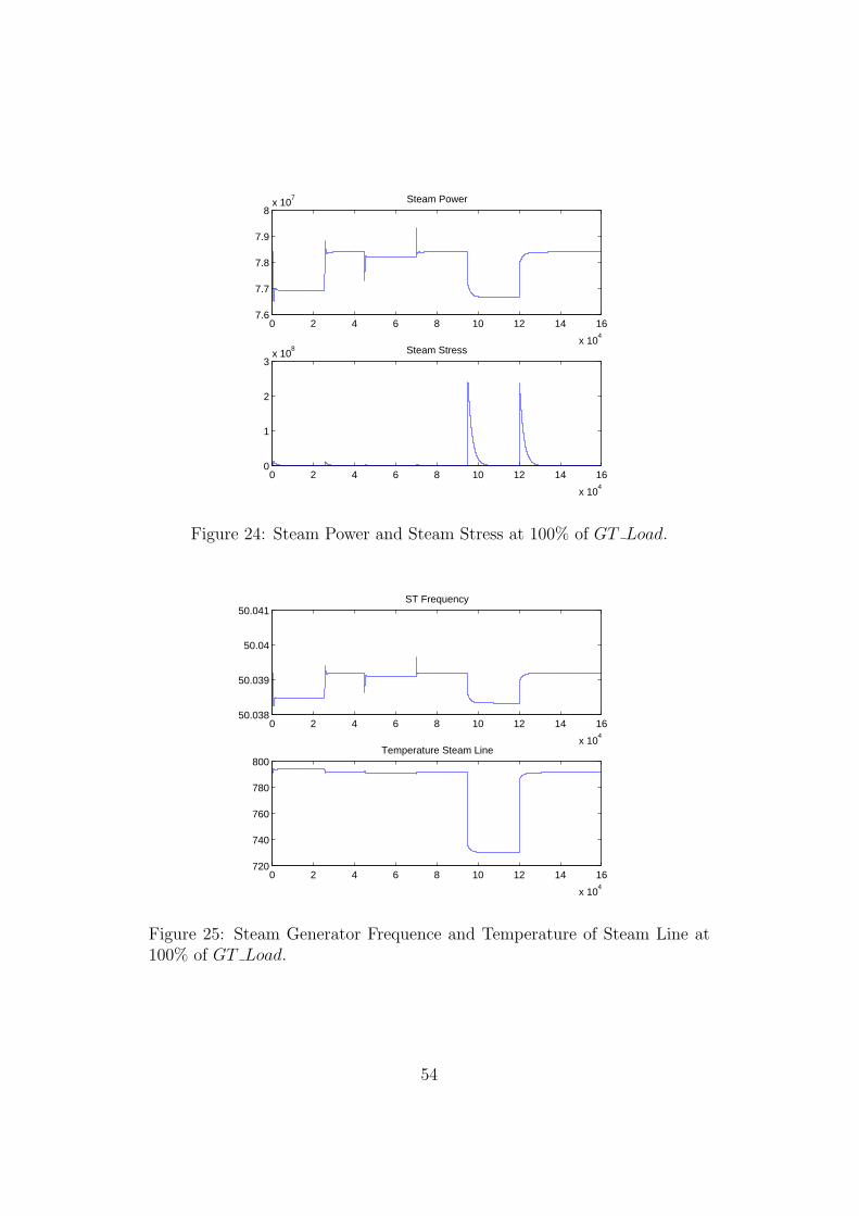
2.3.1 Simulation at 100% of GT Load

An example of the simulations performed to produce the data subsequentlyused for the identification phase is now described. The inputs are thosedescribed in the Figures 18, 19 and 20 and the drum level is controlled witha standard PI regulator. The transients of the main output variables areshown in Figures 21, 22, 23, 24, 25, 26.

49

Point of Work input GT Load Valve ST Feed DSH [kg/s]

100%stable 1 1 0

variation 0.95 0.95 3,209885

75%stable 0.75 1 0

variation 0.7 0.95 3,209885

65%stable 0.65 1 0

variation 0.6 0.95 3,209885

60%stable 0.6 1 0

variation 0.55 0.95 3,209885

57%stable 0.57 1 0

variation 0.52 0.95 3,209885

50%stable 0.5 1 0

variation 0.55 0.95 3,209885

40%stable 0.4 0,872274 0

variation 0.35 0,822274 3,209885

25%stable 0.25 0,872274 0

variation 0.2 0,822274 3,209885

15%stable 0.15 0,286485 0

variation 0.1 0,236485 0,9

Table 10: Inputs for identification.

50

Figure 18: Inputs: example - 1


51


0 2 4 6 8 10 12 14 16

x 104

2.2

2.25

2.3

2.35x 10

8 Gas Turbine Power

0 2 4 6 8 10 12 14 16

x 104

11.7

11.8

11.9

12

12.1

12.2Gas Turbine Fuel

Figure 21: Gas Turbine Power and Gas Turbine Fuel at 100% of GT Load.

52

0 2 4 6 8 10 12 14 16

x 104

−0.02

−0.01

0

0.01

0.02Drum Level

0 2 4 6 8 10 12 14 16

x 104

790

792

794

796Temperature SuperHeater

Figure 22: Drum Level and Temperature of SuperHeater at 100% ofGT Load.

0 2 4 6 8 10 12 14 16

x 104

9.2

9.4

9.6

9.8x 10

6 Steam Pres

0 2 4 6 8 10 12 14 16

x 104

1

1.05

1.1

1.15x 10

8 Header Stress

Figure 23: Steam Pressure and Header Stress at 100% of GT Load.

53

0 2 4 6 8 10 12 14 16

x 104

7.6

7.7

7.8

7.9

8x 10

7 Steam Power

0 2 4 6 8 10 12 14 16

x 104

0

1

2

3x 10

8 Steam Stress

Figure 24: Steam Power and Steam Stress at 100% of GT Load.

0 2 4 6 8 10 12 14 16

x 104

50.038

50.039

50.04

50.041ST Frequency

0 2 4 6 8 10 12 14 16

x 104

720

740

760

780

800Temperature Steam Line

Figure 25: Steam Generator Frequence and Temperature of Steam Line at100% of GT Load.

54

Figure 26: Steam Flow at 100% of GT Load.

2.4 Identification with the Matlab Identification Tool-box

Due to the length of the simulations performed, it is not easy to interpret thecorresponding results and to obtain useful information for the identificationof the local linear models. As a matter of fact, being the input variationsstep changes, a preliminary visual inspection of the output variables cangive a quite precise idea of the order and structure of the linear models tobe estimated and of the main time constants. In order to extract theseinformation from the available data, and to determine the sampling time tobe used in the identification of discrete-time models, a simple Matlab GUIinterface has been developed.The empty GUI is shown in Figure 27: it gives the possibility to load theinput and output variables of interest and to plot the transient response ofthe output in the first six operational points. The use of the GUI is verysimple: first the data must be loaded with the Load Button (the data of allthe simulations are gathered in all load.mat file), then the input and outputvariables must be chosen with two drop down menus. On the left part ofthe screen the steady-state values are also reported for each load. Finally,in order to select the transient of interest, two buttons allow one to specifyif he/she is interested in positive or negative step variations. Finally, a Savebutton is available to save the data. In Figure 28, an example of the use ofthe developed GUI is reported.

The identification of the transfer functions of the local linear models (seeChapter 2.1) has been performed with the Matlab Identification Toolbox, andin particular with the Matlab GUI ident. This toolbox allows one to selectamong different model structures, such as continuous-time or discrete-time,ARX, Output−Error models, and to define the order of the transfer func-tions to be identified.The main criterion adopted in this phase has been to estimate systems of low

55

Figure 27: The developed Matlab GUI.

Figure 28: An example of the Matlab GUI.

56

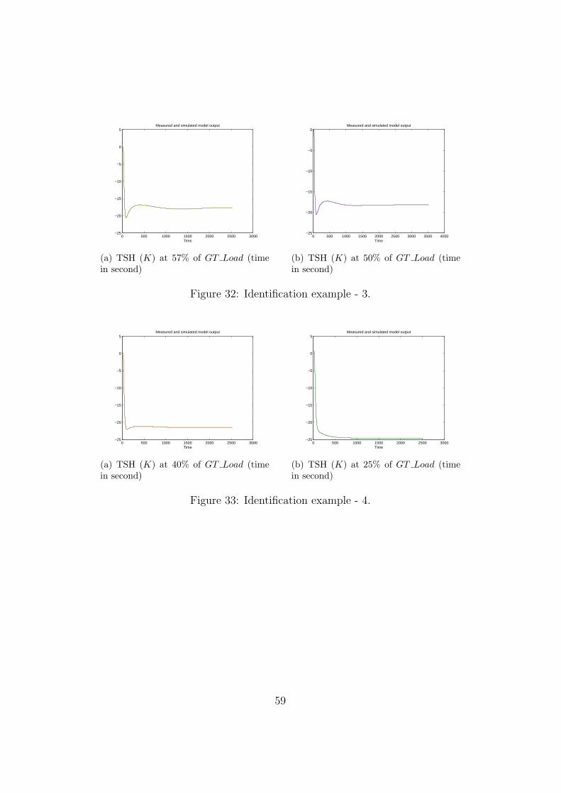
order (first and second), mainly focusing on discrete-time models and ARXand Output Error structures. Indeed, the results achieved could be refined,but they can already be considered as fully satisfactory for the goals of theoverall project.An example of the results obtained with the identification procedure is shownin Figures 29 - 34. In particular, Figure 29 shows the GUI interface with anumber of identified transfer functions between the GT Load and the Tem-perature of SuperHeater (TSH). In these figures the x-axis is the time [s]and the y-axis the temperature [K]. It is important to note that all the valuesare normalized, to obtain better results. The same transfer function is con-sidered in the Figures 30- 34 which compare the transients corresponding tothe simulation data with those provided by the estimated models. In all thefigures the black lines represent the data, while the other lines the identifiedmodels.

Figure 29: Identification GUI for GT Load - TSH.

57

0 500 1000 1500 2000 2500 3000−0.5

0

0.5

1

1.5

2

2.5

3

3.5

Time

Measured and simulated model output

(a) TSH (K) at 100% of GT Load (timein second)

0 500 1000 1500 2000 2500 3000−1

−0.5

0

0.5

1

1.5

2

2.5

3

3.5

4

Time


(b) TSH (K) at 75% of GT Load (timein second)

Figure 30: Identification example - 1.

0 500 1000 1500 2000 2500 3000−1

−0.5

0

0.5

1

1.5

2

2.5

3

3.5

4

Time



0 500 1000 1500 2000 2500 3000−25

−20

−15

−10

−5

0

5

Time




58

0 500 1000 1500 2000 2500 3000−25

−20

−15

−10

−5

0

5

Time



0 500 1000 1500 2000 2500 3000 3500 4000−25

−20

−15

−10

−5

0

Time




0 500 1000 1500 2000 2500 3000−25

−20

−15

−10

−5

0

5

Time



0 500 1000 1500 2000 2500 3000−25

−20

−15

−10

−5

0

5

Time




59

0 500 1000 1500 2000 2500 3000−30

−25

−20

−15

−10

−5

0

Time




2.5 Building the interpolation scheme withMatlab Simulink

Once all the transfer function describing the input-output relations at theconsidered operating points have been estimated, the adopted approach re-quires to build the overall model, including the membership functions. This issimple in the Simulink environment by means of the Fuzzy Systems toolbox,where a specific block for the definition of the membership functions is avail-able. Then, a Simulink model can easily be built for any output variable. Asan example, Figure 35 shows the Simulink model for the temperature TSH:it has the three system inputs, the main subsystem block and the output.The main block is expanded in Figure 36, where it is possible to see the blockscorresponding to the local linear models at any load, the block computingthe membership functions and the connections among them. The weights(outputs of the membership functions) allow one to compute the final out-put as the interpolation of the contributions of the local models. The blockcomputing the membership functions is expanded in Figure 37, while thelocal model at the 100% of the load is shown in Figure 38), which containsthe identified transfer functions (see Figure 39). Note in particular that inthe implementation of the transfer functions it is possible to use the blocksldmodel, which allow one to use the models identified with the ident toolboxwithout any further elaboration.

The procedure now sketched to obtain the model of the variable TSHcan be repeated for each output variable. In this Thesis, the models of fourvariables have been identified:

� TSH: temperature of superheater;

60

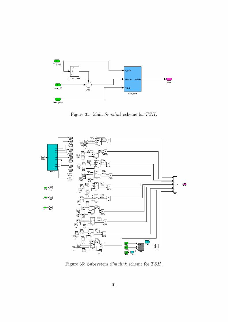
Figure 35: Main Simulink scheme for TSH.

Figure 36: Subsystem Simulink scheme for TSH.

61

Figure 37: Membership functions Simulink scheme.

Figure 38: Local Simulink subsystem for TSH at 100% of GT Load.

62

Figure 39: Detail of Simulink scheme to build the local model.

� ST Press: steam pressure;

� Header Stress: stress of the header;

� ST Stress: st*ress inside the steam turbine.

A possible future development can concern the modeling of all the plantoutput variables, paying attention to the fact that the power produced bythe gas turbine and the gas turbine fuel have a very fast dynamics withrespect to the other outputs. Then, these variables can be modeled withsimple static relations.The final Simulink scheme for the identified variables is shown in Figure 40.

63

Figure 40: Simulink scheme for all identified variables.

64

3 Chapter 3: Validation of the identified mod-

els

The validation of the identified model developed in Matlab/Simulink hasbeen performed by comparing its behavour with the one of the original Mod-elica model used to generate the data. Different sets of data have beenconsidered to compare the two models both locally and with respect to largevariations of the GT Load over the whole operating range of the CCPP. Inthis second case, positive and negative ramp variations, from the 15% of theload to full load and viceversa, have been imposed.In the following Figures 41, 42, 43, 44, 45 and 46 the transients of the steampressure due to small variations of theGT Load starting from different steadystate operating conditions are reported. In these figures, and in all the figuresof the chapter, the blue line shows the transients computed with Dymola,while the green line those produced by the Simulink model.

−1500 −1000 −500 0 500 1000 1500 2000 2500 3000 35009.25

9.3

9.35

9.4

9.45

9.5

9.55x 10

6

[s]

[Pa]

Figure 41: GT Load - ST Pressure transient at 100%.

65

−1500 −1000 −500 0 500 1000 1500 2000 2500 3000 35008.25

8.3

8.35

8.4

8.45

8.5

8.55x 10

6

[s]

[Pa]


−2000 −1000 0 1000 2000 3000 40007.3

7.4

7.5

7.6

7.7

7.8

7.9

8x 10

6

[s]

[Pa]


66

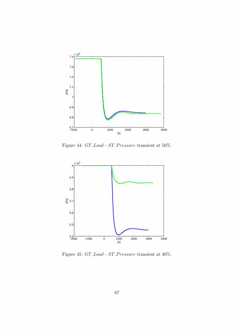
−1000 0 1000 2000 3000 40006.7

6.8

6.9

7

7.1

7.2

7.3

7.4x 10

6

[s]

[Pa]


−2000 −1000 0 1000 2000 3000 40005.4

5.5

5.6

5.7

5.8

5.9

6x 10

6

[s]

[Pa]


67

−1500 −1000 −500 0 500 1000 1500 2000 2500 3000 35004.8

5

5.2

5.4

5.6

5.8

6x 10

6

[s]

[Pa]


A short comment must be done for the figure which represent the variationof the load from 40% to 35%: is possible to see a gap from Simulink andDymola response. This because the dynamic of the valve is modelized onlywith a look-up table in function of the load, which approx the behavior ofthe valve. To have a better model the only way is to improve this function,with more point. By the way is not much important, because at this pointof work the pressure controller is online. The transients produced by theopening of the admission valve in the two models are reported in Figures 47,48, 49, 50, 51 and 52.

68

0 1000 2000 3000 4000 50009.5

9.55

9.6

9.65x 10

6

[s]

[Pa]

Figure 47: V alve ST - ST Pressure transient at 100%.

0 1000 2000 3000 4000 50008.54

8.56

8.58

8.6

8.62

8.64

8.66

8.68x 10

6

[s]

[Pa]


69

0 1000 2000 3000 4000 50007.9

7.92

7.94

7.96

7.98

8

8.02

8.04x 10

6

[s]

[Pa]


0 1000 2000 3000 4000 50006.82

6.84

6.86

6.88

6.9

6.92

6.94x 10

6

[s]

[Pa]


70

500 1000 1500 2000 2500 3000 3500 4000 4500 50005.98

6

6.02

6.04

6.06

6.08

6.1

6.12

6.14x 10

6

[s]

[Pa]

Figure 51: V alve ST - ST Pressuree transient at 40%.

500 1000 1500 2000 2500 3000 3500 4000 4500 50005.9

6

6.1

6.2

6.3

6.4

6.5

6.6

6.7

6.8x 10

6

[s]

[Pa]


The small difference (about 0.2 bar) in Figure 49 between the responses inDymola and Simulink is due to the interpolation between local linear modelsin Simulink: near the regime corresponding to the 60% of the load, manylocal models have been used to properly reproduce the change of sign of the

71

gain in some transfer functions; correspondingly, the membership functionsare very dense. However, the difference between the two models is quite smalland fully acceptable for the scopes of this work.The Figures 53, 54, 55, 56, 57 and 58 show the transient between theFeed DSH and the steam pressure.

0 0.5 1 1.5 2

x 104

9.45

9.46

9.47

9.48

9.49

9.5

9.51x 10

6

[s]

[Pa]

Figure 53: Feed DSH - ST Pressure transient at 100%.

72

0 0.5 1 1.5 2

x 104

8.49

8.5

8.51

8.52

8.53

8.54

8.55x 10

6

[s]

[Pa]


0 0.5 1 1.5 2

x 104

7.87

7.88

7.89

7.9

7.91

7.92

7.93x 10

6

[s]

[Pa]


73

0 0.5 1 1.5 2

x 104

6.77

6.78

6.79

6.8

6.81

6.82

6.83

6.84x 10

6

[s]

[Pa]


0 0.5 1 1.5 2

x 104

5.91

5.92

5.93

5.94

5.95

5.96

5.97

5.98

5.99

6x 10

6

[s]

[Pa]


74

0 0.5 1 1.5 2

x 104

5.75

5.8

5.85

5.9

5.95

6x 10

6

[s]

[Pa]


Also in this case, it is possible to note a small gap between the Dymolaand the Simulink responses at 60% of the load, due to the same causes pre-viously described. On the contrary, Figure 58 shows that the two modelshave a significantly different behavior at low load. However, this difference(about 2 bar) is not critical, in fact like at 40% of load, in these conditionsa pressure controller is normally online.

The final results are referred to the large ramp variations corresponding tothe shutdown (Figure 59) and to the start-up (Figure 60) phases. Bothare encompassed between 100% and 15% of GT Load. The transients of thefour outputs analyzed are shown in Figures 61, 62, 63 and 64 for the negativeramp, and in Figures 65, 66, 67, 68 for the positive one.

75

0 1 2 3 4 5 6 7 8 9 10

x 104

0

0.5

1

1.5

2

2.5x 10

8

[s]

[MW

]

Figure 59: Shutdown ramp.

0 0.5 1 1.5 2 2.5 3 3.5 4 4.5 5

x 104

0

0.5

1

1.5

2

2.5x 10

8

[s]

[MW

]

Figure 60: Start-up ramp.

76

0 2 4 6 8 10

x 104

600

650

700

750

800

850TSH

[s]

[K]

Figure 61: Shutdown temperature of superheater.

0 2 4 6 8 10

x 104

5.5

6

6.5

7

7.5

8

8.5

9

9.5

10x 10

6 ST Pressure

[s]

[Pa]

Figure 62: Shutdown steam pressure.

77

0 2 4 6 8 10

x 104

6.5

7

7.5

8

8.5

9

9.5

10

10.5

11x 10

7 Header Stress

[s]

[Pa]

Figure 63: Shutdown header stress.

0 2 4 6 8 10

x 104

0

0.5

1

1.5

2

2.5

3

3.5x 10

8 ST Stress

[s]

[Pa]

Figure 64: Shutdown steam turbine stress.

78

0 1 2 3 4 5

x 104

600

650

700

750

800

850TSH

[s]

[K]

Figure 65: Start-up temperature of superheater.

0 1 2 3 4 5

x 104

5.5

6

6.5

7

7.5

8

8.5

9

9.5

10x 10

6 ST Pressure

[s]

[Pa]

Figure 66: Start-up steam pressure.

79

0 1 2 3 4 5

x 104

5

6

7

8

9

10

11

12x 10

7 Header Stress

[s]

[Pa]

Figure 67: Start-up header stress.

0 1 2 3 4 5

x 104

0

0.5

1

1.5

2

2.5

3

3.5x 10

8 ST Stress

[s]

[Pa]

Figure 68: Start-up steam turbine stress.

It is possible to note that the responses to the two load variations aredifferent. In the shutdown case, the Simulink responses fit very well theDymola data. This is due to the fact that these data have been used forthe definition of the membership functions. Therefore, the comparison of the

80

shutdown transients cannot be properly considered as a validation test. Onthe contrary, the analysis of the start-up experiments is made on data notused to identify the interpolated model. As expected (recall that the Dymolamodel is highly nonlinear), the fitting is slightly worse than the previous one.The worst response is shown in Figure 68, where the Simulink model is notable to properly reproduce the peak stress.

81

4 Chapter 4: Optimization

This chapter describes the optimization procedure developed to determinethe GT Load profile minimizing the start-up time while fulfilling a number ofconstraints on the main process variables. More specifically, it is required thatduring the start-up phase temperatures, pressures and stresses remain intoprescribed limits for safety and economical reasons. The approach is basedon the definition of a minimum-time control problem subject to constraints.Its solution is obtained by means of the joint use of the Simulink simulatorpreviously developed and of the Matlab Optimization Toolbox.

4.1 Minimum-time optimization problem

The model of the Combined Cycle Power Plant can be given the general formof a set of continuous-time differential equations:

x = f(x(t), L(t))

where x is the state vector, which contains the plant variables, and L repre-sents the gas turbine load.Denote by t0 the initial time instant of the start-up procedure (convention-ally it can be set t0 = 0) and by tf the final one. As for the load profile, itmust be selected so that L(t0) = Lm and L(tf ) = LM , Lm and LM being theinitial and final (full) load.Assume now that the load is described by an increasing function L(t, q)satisfying the boundary conditions above stated and where q is a vector ofunknown parameters, which have to be selected through an optimization pro-cedure. Then, the problem of computing the optimal load profile consists offinding the value of the parameter vector q, together with the final time tf ,which solves the following optimization problem:

minq,tf

J =

∫ tf

t0

dt (51)

subject to the constraints:

x = f(x(t), L(t, q)) (52)

L(tf , q) ≥ LM − ε1 (53)

|f(x(tf ), L(tf , q))| ≤ ε2 (54)

h(x(t)) ≤ 0, t0 ≤ t ≤ tf (55)

82

where ε1 and ε2 are arbitrary small values (ideally equal to zero) and thecorresponding constraints are included to guarantee that at time tf the sys-tem is (almost) in stationary conditions and has reached (almost) full load.The last (vector) constraint includes, in general form, all the constraints tobe imposed to the plant variables, in particular on the stresses, during thestart-up procedure.Many functions L(t, q) can be chosen, such as sigmoid functions. In thiswork, the following Hill function has been chosen:

L(t, q) = Lm + (LM − Lm)th

th + kh(56)

where q = [h k] is the parameter vector to be determined through the op-timization procedure. An example of Hill function for different values of itsparameters is shown in Figure 69.

0 0.5 1 1.5 2 2.5 3

x 104

0.1

0.2

0.3

0.4

0.5

0.6

0.7

0.8

0.9

1

[s]

perc

enta

ge o

f loa

d

Figure 69: Hill function with Lm=0.15, LM=1, t0=0, tf=30000, k=2 andh=5000 (blue), k=4 h=5000 (green), k=6 h=5000 (red)

4.2 Matlab Algorithm

For the solution of the minimum-time optimization problem, a program hasbeen created in Matlab. This program is based on the minimization func-tion fmincon, available in the Matlab Optimization Toolbox, which solves

83

nonlinear constrained minimization problems starting from an initial guessof the solution.

Fmincon has the following structure:

x = fmincon(@myfun, x0, A, b, Aeq, beq, lb, ub, @mycon)

where myfun is the function to be minimized, which accepts a vector x andreturns a scalar f , the objective function evaluated at x. With the “@” sym-bols, myfun is specified as a function defined through a file. A and Aeqare linear constraint matrices, b and beq their corresponding vectors. In ourcase, since the problem is non-linear, A, Aeq, b and beq are empty (in theMatlab syntax they are defined as empty matrices as follows: A = [ ]). Thevectors lb and ub indicate, respectively, the lower and the upper bounds ofthe unknown elements of x, i.e. of the variables to be determined by theoptimization algorithm. In the mycon function all nonlinear constraints aredefined.

In order to solve the optimization problem for the CCPP, three files havebeen created:

1. opt hill

2. con hill

3. fun hill

The opt hill file is the main program which defines and manages the opti-mization problem. Its code is the following:

c l e a r a l lload t o t a l . matx0=[0.001 5 30000 ] ;lb =[0 2 .3 10800 ] ;ub=[0.0051 10 100000 ] ;A= [ ] ;b= [ ] ;Aeq= [ ] ;beq = [ ] ;opt imset ( ’ fmincon ’ ) ;opts=opt imset ( ’ Display ’ , ’ I t e r ’ , ’ TolFun ’ , 1 0 ˆ ( − 6 ) , . . .

’MaxFunEvals ’ , 1 000 , ’ MaxIter ’ , 1 0000 , ’ TolX ’ , 10ˆ( −20) ) ;[K, fva l , e x i t f l a g ]= fmincon (@(K) f u n h i l l (K) , x0 ,A, b , Aeq ,

beq , lb , ub ,@(K) c o n h i l l (K) ) ;

84

This file fixes the initial values (for example, the initial guess for the final timeof the start-up phase is set to 30000 seconds, see [12], [9]), and the upper andlower bounds for the parameters h and k of the Hill function. In call of fmincon,the name of the file computing the performance index to be minimized is speci-fied (fun hill), together with the name of the function computing the constraints(con hill). With the optimset instruction some options for fmincon are set.

The file fun hill computes the cost function, i.e. the final time of the start-up:

func t i on J = f u n h i l l (K)J=K( 3 ) ;

The file is composed only by one row of code because the cost function correspondsto one of the parameters to be determined.

The third file, con hill, computes the constraints to be fulfilled in the optimizationproblem. Its code is:

f unc t i on [C, Ceq ] = c o n h i l l 1 (K)%% H i l l f unc t i onKlm=0.15;lM=1;tsim =(0 :1 :K( 3 ) ) ;f o r i =1: l ength ( tsim )

L( i )=lm+(lM−lm )* ( ( ts im ( i )ˆ (K(1)*1000) )/( tsim ( i )ˆ (K(1)*1000)+(K(2)*1000)ˆ(K( 1 ) * 1 0 0 0 ) ) ) ;

endtsim =(0 :1 :K( 3 ) ) ’ ;l oadgt=L ’ ;p l o t ( tsim ,L ) ;

%% s imu la t ing model[ t1 ,X,Y]=sim ( ’ tota lmodel ’ , [ ts im (1) tsim ( end ) ] ,

[ ] , [ tsim , loadgt ] ) ;

DERI=Y( end , : )−Y( end −1 , : ) ;STRESSMAXHEADER=max(Y( : , 1 ) )STRESSMAX STEAM=max(Y( : , 4 ) )

ERR=DERI*DERI’

Ceq= [ ] ;C=ERR−1;

85

C=[C;STRESSMAXHEADER−11e +7] ;C=[C;STRESSMAX STEAM−2.25 e +8] ;C=[C;−L( end)+lM−0.005]

In the first part, the file computes the Hill function, i.e. the GT load, correspond-ing the current values of the optimization variables, which will be the input for theSimulink model used to simulate the plant behavior. Then, the Simulink model isrun and, based on the computed transients of the plant variables, the constraintson Header Stress and Steam Stress are evaluated, together with the constraintswhich require to reach almost the steady state conditions at the end of the simu-lation.To obtain good results, many simulations are needed; a good idea is to start dif-ferent simulations with different bounds and initial states, so as to explore all thefeasibility space. The time for one simulation is about five minutes, but it stronglydepends on the inputs. Another important aspect to consider is that fmincon isnot an efficient routine: sometimes problems occur and the tests crash. This typi-cally happens when Matlab tries to move from a set of safe values. The weaknessof fmincon algorithm is balanced by its simplicity. Different solvers and optimiza-tion tools, such as Tomlab, should be tested to make the optimization phase morereliable and efficient.

4.3 Optimization Results

After the processing of the system with fmincon, a solution is founded which re-duce the time of start-up and maintain the stresses under the imposed constraints.With this solution the system also arrive near 100% of GT Load (note that inconstraints there is a little parameter ε that allow the system to stay under thefull load. This parameter is very small, but this solution allow Matlab to obtainmore simply the result).The functions built for the optimization give this optimal K vector of parameter:

K = 1.0e+ 004 ∗ [0.000000327902446 0.000233591945258 1.231463112769526]

where the two first number are Hill function parameters, and the third is the timeof simulation. These parameters generate the Hill function showed in Figure 70,which represent the optimal load curve.

Starting from initial condition (x0 = [10 5000 30000], then 30000 seconds tostart-up the plant and arrive at full load) the optimization tool calculate a functionthat allow to start-up the plant in only 12315 seconds. In figures 71, 72, 73 and 74,whichs represents respectively the temperature of superheater, the steam pressure,the header stress and the steam turbine rotor stress.

In these figures is possible to note how the curves reach, in less time, the fullload, with a good behavior for temperature of superheater and for steam pressure.Header stress and steam turbine rotor stress respect the imposed constraints, and

86

0 2000 4000 6000 8000 10000 12000 140000.1

0.2

0.3

0.4

0.5

0.6

0.7

0.8

0.9

1

[s]

load

per

cent

age

Figure 70: Optimal load curve

0 2000 4000 6000 8000 10000 12000 14000600

650

700

750

800

850TSH

[s]

[K]

Figure 71: Optimized temperature of superHeater (TSH)

87

0 2000 4000 6000 8000 10000 12000 140005.5

6

6.5

7

7.5

8

8.5

9

9.5x 10

6 ST Pressure

[s]

[Pa]

Figure 72: Optimized steam pressure

0 2000 4000 6000 8000 10000 12000 140004

5

6

7

8

9

10

11x 10

7 Header Stress

[s]

[Pa]

Figure 73: Optimized header stress

88

0 2000 4000 6000 8000 10000 12000 140000

0.5

1

1.5

2

2.5x 10

8 ST Stress

[s]

[Pa]

Figure 74: Optimized steam turbine rotor stress

for the first one values are lower than the stress generate from the load ramp.The successive step is to validate this solution on Dymola model, to observe if theoptimization algorithm is even good. The same load is given on Dymola modelas a input, with the same admission valve dynamic even imposed by the load.Unfortunately the results are not very well as in Simulink model. Temperatureof superheater, steam pressure and headerstress are very similar, as is possibile tosee in Figures 75, 76 and 77, and respect the imposed constraints, as in Simulinkmodel.

Steam stress has a very different behavior in Dymola model, as is possibleto see in Figure 78: here the stress doesn’t respect the constraint, reaching veryhigh value (about 700 milions of Pascal instead 200). Probably this difference isgiven from the problem highlighted in Chapter 3, that is the non linearities of themodel. The problems in Chapter 3 whichs does not allow to obtain a very goodidentification in start-up phase for steam stress are here mirrored, producing thisbad result. In a future development a better identification can probably solve this,but will be necessary restart the optimization algorithm to obtain new values forthe GT Load

89

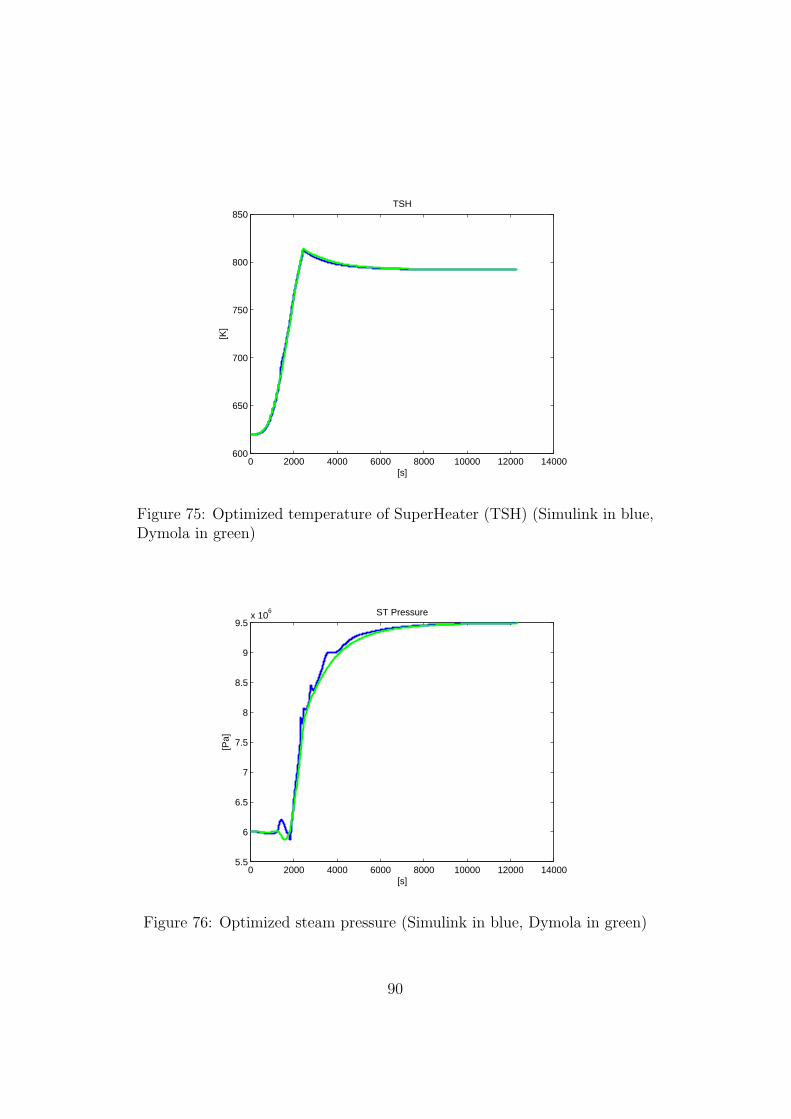
0 2000 4000 6000 8000 10000 12000 14000600

650

700

750

800

850TSH

[s]

[K]

Figure 75: Optimized temperature of SuperHeater (TSH) (Simulink in blue,Dymola in green)

0 2000 4000 6000 8000 10000 12000 140005.5

6

6.5

7

7.5

8

8.5

9

9.5x 10

6 ST Pressure

[s]

[Pa]

Figure 76: Optimized steam pressure (Simulink in blue, Dymola in green)

90

0 2000 4000 6000 8000 10000 12000 140004

5

6

7

8

9

10

11x 10

7 Header Stress

[s]

[Pa]

Figure 77: Optimized header stress (Simulink in blue, Dymola in green)

0 2000 4000 6000 8000 10000 12000 140000

1

2

3

4

5

6

7x 10

8 ST Stress

[s]

[Pa]

Figure 78: Optimized steam stress (Simulink in blue, Dymola in green)

91

5 Chapter 5: Conclusion

In this Thesis, a simplified model of a CCPP has been developed in the Mat-lab/Simulink environment, starting from a detailed Dymola model already avail-able. The model has been derived by interpolation of a number of estimated linearmodels with local validity, and has been used to optimize the start-up phase of theplant. The simplified model has been validated with respect to large ramp-typevariations of the gas turbine load, starting from low loads (15% of the full load)to full load conditions and vice versa. The transients of the main plant variables,namely temperatures, pressures and thermal stresses, have shown in general anexcellent correspondence with those provided by the original Dymola model. Thisis a a significant result, since the behavior of the system is highly nonlinear andasymmetric for positive or negative variations of the load.The second part of the Thesis has considered the design of the load profile to befollowed during the start-up phase to reduce the overall time required to reach fullload conditions while maintaining the process variables within prescribed ranges.This requirement is particularly important for the lifetime of the plant, in partic-ular for what concerns the thermal stresses. This problem has been formulatedas a mathematical programming problem, and more specifically, as a constrainedminimum time problem. The load profile has been assumed to have the form ofa Hill function, i.e. a parametrized continuous and increasing function, whose pa-rameters are the unknowns of the optimization problem, together with the finaltime. The solution of this minimum time problem has been found with standardoptimization tools available in the Matlab/Simulink environment. The computedoptimal load profile has then been applied to the estimated and interpolated model;this test has verified that the start-up time is effectively reduced with respect tostandard procedures and the constraints on the stresses are fulfilled. Finally, thecomputed optimal profile has been used to simulate the start-up with the Dymolamodel. The results achieved are largely expected, and confirm that the time re-quired to reach full load conditions is reduced maintaining most of the variablesin the prescribed limits. The only exception is due to the behavior of one of thestresses, whose value is too high. This is probably due to a not sufficiently preciseidentified model for that variable, and it is believed that a more reliable estimatedmodel could completely solve the problem.In conclusion, the approach developed in this Thesis can be considered efficient,and could probably be extended to analyze other energy problems related to plantswith a strongly non linear behavior. Obviously, as it is standard in the developmentof a new approach, there are many possible future developments, such as:

� the development of a bigger model, which describes all the plant variables(at the moment only a subset of significant variables has been consideredin the development of the identified model). This is very easy, because it isnecessary only to repeat the identification of the local linear models and theirinterpolation for any new variable, while maintaining the same interpolation

92

structure.

� Consider the possibility to use other input variables in the optimizationprocedure.

� Include a model of the emissions of the gas turbine and constraint their valuein the optimization problem for the determination of the load profile. Thiswill become more and more important in the future, in view of the tightlegal requirements on the emission of CCPP.

� Use an optimization procedure to tune the parameters of the membershipfunctions which are used in the interpolation of local linear models. Thiswould allow to save a lot of time in the design phase of the model, andprobably would improve the achieved solutions.

� Use more efficient optimization tools than those applied in this work (thefunction fmincon in the Matlab optimization toolbox).

� Consider other load profiles. The Hill function is a flexible and easy choice,with a small number of parameters to be computed, but other functionscould be considered. Another possibility would be to consider the cascadeof two Hill functions to replicate the shape usually followed in industrialplants.

� Extend the approach to other energy system, developing a set of modelsvery easy to simulate. This can be very convenient also in the project phase,because it gives the possibility to have simple and fast tools for simulation,control design and optimization.

93

A Simulations Procedure

This appendix reports a short manual describing how to perform the simulationswith Dymola and hao to manage all the files developed. The first subsection,describes the methodology to obtain results from the SUPELEC Dymola model,in order to have similar results at different loads.

A.1 Simulations on Dymola

The Modelica model provided by SUPELEC has two possible initialization points:full load conditions or at 7.5% of load. In this case, the initialization is set by thehot start up.txt file, available in SUPELEC package, see [15]. In this section it isshown how to perform different simulations starting from steady-state conditionscharacterized by a constant load in the range 7.5%-100%. The simulations are al-ways performed with a local regulator controlling the drum level. This is necessaryfor the identification procedure described in the following chapter to eliminate theintegrating behavior of the level, which can cause troubles in the simulation phase.Moreover, also a regulator controlling the steam pressure is used to guarantee thatthis variable remains into prescribed limits.

The procedure to run the simulations is easy, but must be strictly followed toavoid errors and false results. As an example, in the following it is described howto simulate the system at values of the load greater or equal to the the 50%:

1. load the model, with the drum level in closed-loop and at the 100% of theload, with the file dsin.txt of default parameters provided by SUPELEC andwith the file dsu.txt of constant inputs (the values of the variables at thisoperating point are presented in a table reported below);

2. “translate” the model in Dymola and run a very long simulation (for exampleof 100000 seconds) in Dymola, to obtain the steady-state at 100% of the load(see Figure 79 on how to set the simulation time);

3. in the folder where the model is placed, there is now a file called dsfinal.txt,which represents the final state at the end of the simulation. Copy andrename it as full load controlled.txt ;

4. choose the operating point of interest. To do this, the model needs a newdsu.txt file, which, according to a ramp behavior, allows to reach the selectedoperational point. With this new input file (which must be placed in thesame folder of the model), the Modelica model must be re-translated andre-simulated to generate a new initialization .txt file (it is important to payattention at the settings of the initial conditions in Dymola, see Figure 80);

5. as before, the dsfinal.txt file represents the final state at the required loadlevel. It is more useful to save this file with another name, for example

94

loadpercentage.txt. In Dymola it is also possible to find the stable value ofthe variable Feed Drum at the considered load level;

6. with the file previously created, the initial conditions at desired operatingpoint can be loaded. Now it is possible to perturb the system with a lo-cal transient near the chosen working point with a new dsu.txt file, whichcontains the perturbation inputs;

7. the results of the simulations are stored in the file model name results.mat.This file is very huge for long simulations. To avoid this problem, is necessaryto select, in “Dymola simulation setup”, only the input and output variablesin the menu. In this way internal and auxiliary variables are not saved inthe file of the results.

The procedure to run the simulation under of 50% of the load is similar, butattention must be paid to use the system with two control loops (level and pres-sure). In this case, not only the stable value of the Feed Drum must be found atdifferent loads, but also the opening of the valve controlling the steam pressure.In fact, the pressure loop is closed on the admission valve.

Figure 79: How to set the time in Dymola.

A.2 Files manual

The target to this part of the appendix is to become easy the work on the thesisfiles. A lot of files have been generated with Dymola, Matlab and Simulink: a

95

Figure 80: How to import the state in Dymola.

little manual to understand how the file are can be very useful.In the main Thesis folder there are:

� Dymola Simulations

� GUI

� Identifications

� Simulink

In Dymola simulations folder all the different simulations made with Dymola havebeen gathered. There are Closed Loop1 and Closed Loop2, whichs contain thetries to obtain the states at different load necessary to initialize the model (as isexplained in A.1. In this folder another one is contained, called Open Loop: insideof this all different simulations with square wave are gathered. It is possible tofind two different type of these, one with the total open loop model, one with theclosed loop model on the drum level. This last it is considered for the identificationand for all the thesis work.In GUI folder are stored all the data from simulations, and there is the code torun the dedicated GUI. With Matlab is sufficient run the fdtgui2.m file to start it.How is explained in Chapter 2, is necessary to load the allload.mat file to see thelocal transitory.In Identifications folder are gathered all the identification done with Matlab Iden-tification ToolBox. The “.sid” files can be loaded in ident mask to see directly thedifferent identifications. To facilitate the read of these files, all are called like out-put input first. In this way is very easy take the proper variable to analyze. Inside

96

of this folder, others two are present: in one of this there are some Matlab scriptto obtain the data for the identifications, in another one the Matlab workspacedata to start the them. Because the inputs are three and the outputs for, twelvefiles have been generated.In Simulink folder are stored all the Simulink plant realized to reproduce the Dy-mola model in Matlab. There are one folder for each reconstruited output: thischoice is very good, because is better tune every model alone. This avoid a lotof problems in project phase. The Total folder store the model which assemblethe single output models. Optimiz and Optimiz2 contain the code to start theoptimization phase, the only difference between the first from the second is ableto launch many simulations.A little precisation to work on Simulink: all developed models require the loadof properly workspace file, that contains all the ldmodel form (the local transferfunction). These are present in every folder and also in workspace folder.

97

References

[1] Mathmodelica.

[2] Openmodelica.

[3] Dynasim AB, Dymola v. 7.2.

[4] Claudio Aurora, Power plants: Modelling, simulation and control, Ph.D. the-sis, University of Pavia, 2004.

[5] Automatica 31, Identification of nonlinear system structure and parametersusing regime decomposition, 1995.

[6] R.D. Bell and K.J. Astrom, Automatica, 2000.

[7] Francesco Casella, Materiale didattico corso modellistica e controllo dei pro-cessi continui e delle reti di pubblica utilita.

[8] Francesco Casella and Alberto Leva, Modelling of thermo-hydraulic powergeneration processes using modelica, mathematical and computer modellingof dynamical systems, v. 12, n. 1, pp. 19-33, 2006.

[9] Francesco Casella and Riccardo Scattolini, Procedure di esercizio innovativeper la gestione ottimale dei gruppi di produzione in fase di avviamento, re-lazione finale, Tech. report, Dipartimento di Elettronica e informazione, Po-litecnico di Milano.

[10] DyOS, Dyos user manual, release 2.1, Aachen University, 2002.

[11] B. A. Foss and T. A. Johansen, Constructing narmax models using armaxmodels, Int. J. Control, 1993.

[12] Morthazavi Hesam, Optimization of the startup time in a combined cyclepower plant considering the thermo mechanical stresses developed in the steamturbine, Master’s thesis, Politecnico di Milano, 2006.

[13] C. Maffezzoni, Dinamica dei generatori a vapore, Hartmann & Braun, 1988.

[14] Modelica Conference, Modelica open library for power plant simulation: de-sign and experimental validation, 2003.

[15] Adrian Tica, One pressure level ccpp model, Tech. report, SUPELEC, Decem-ber 2009.

98

Control and optimization of the start-up of a combined cycle … · · 2013-03-05POLITECNICO DI...

Documents

Transcript of Control and optimization of the start-up of a combined cycle … · · 2013-03-05POLITECNICO DI...