Control and optimization of ecosystems in bioreactors for ...
150
HAL Id: tel-00850420 https://tel.archives-ouvertes.fr/tel-00850420 Submitted on 21 Aug 2013 HAL is a multi-disciplinary open access archive for the deposit and dissemination of sci- entific research documents, whether they are pub- lished or not. The documents may come from teaching and research institutions in France or abroad, or from public or private research centers. L’archive ouverte pluridisciplinaire HAL, est destinée au dépôt et à la diffusion de documents scientifiques de niveau recherche, publiés ou non, émanant des établissements d’enseignement et de recherche français ou étrangers, des laboratoires publics ou privés. Control and optimization of ecosystems in bioreactors for bioenergy production Pierre Masci To cite this version: Pierre Masci. Control and optimization of ecosystems in bioreactors for bioenergy production. Auto- matic. Université Nice Sophia Antipolis, 2010. English. tel-00850420
Transcript of Control and optimization of ecosystems in bioreactors for ...

HAL Id: tel-00850420https://tel.archives-ouvertes.fr/tel-00850420
Submitted on 21 Aug 2013
HAL is a multi-disciplinary open accessarchive for the deposit and dissemination of sci-entific research documents, whether they are pub-lished or not. The documents may come fromteaching and research institutions in France orabroad, or from public or private research centers.
L’archive ouverte pluridisciplinaire HAL, estdestinée au dépôt et à la diffusion de documentsscientifiques de niveau recherche, publiés ou non,émanant des établissements d’enseignement et derecherche français ou étrangers, des laboratoirespublics ou privés.
Control and optimization of ecosystems in bioreactorsfor bioenergy production
Pierre Masci
To cite this version:Pierre Masci. Control and optimization of ecosystems in bioreactors for bioenergy production. Auto-matic. Université Nice Sophia Antipolis, 2010. English. �tel-00850420�

���������
�����������
ABC��DE�F��C��FED�F�������B������
�����������������A�
�A��B�������A�������C�CA��� �B���C����DEAFF��F�����F�����F�������F��C��E���F��DE���E�
����������F��C��������������������C��������F���A�����C���������F���A���������F�
�����B�������A��
D��E������������F���F���D������������������FE����
�D��!D����"�DE�F�F#��FD��D$��%D�&������F��'FD!��%�D!��$D!�'FD���!(&�E!D")%�FD�
���������D��
�A����������������A��� � !"��������#!���DF�A��������F��$%���E�����&� ��'����("!#�!%�����EF)C���'�����&�*�+�+��E�B! B#�!%
���������F���A��,�A�F�����������ABA
*)!&�+��$� ��'����("!#�!%��������������������������%!���#!���DF�A�������������������������������'�F�
�$�������-�#%"�. /."!�����������������$��/��'����+�����F� ����������!�'��0���$�*�+�+��E���1"#���������������������������!���#!���D�E��&����������������������������!�'��0��
�$�BF����F�! (2"% ��������������������������������$��/��'$�����A���������������"3��������$�4���)�A���F�A��� BB��2"�����������$��/��'����+���3)���������������������"3��������$�B�5��( /B�!�# ��������!���*!"�"!�#��������������������������"3������
��'������������6��$�*�+�+��E�B! B#�!%������������!���#!���DF�A��������������'�F�


/#�-"!D��"�%"�#��")D �7����#��� 2�D
��� �������BC ��������A�����������A� �,������ -A��B�C��A������� C������A�C��A
���������
�FC��F������������������
�D%��)!�����%F��%��
����8/��'����+����#�E�)DF�A��������F��
%�E������6��C�F�����C���������������C�D�����������������
��+���+�����FC���C�����
CD�����EF���
�D��!.������DE�F�F���FD��"/0%D�&��1�������'FD!0�%��)!��ED)!����E!D")%�FD��"��'FD0��!(F�
�A9�������+������ �D�D�������F�������������D�������� ��!��D��"�#"�F��������������$��%����F����&D��F'(D���D������)�(��#E#��
FC���C�����,����������ABA
*)!&�+��$� ��'����("!#�!%������������������������%!���#!���DF�A���������������������������%���E��C�
�$�������-�#%"�. /."!���������������$��/��'����+�����F� �����������������!���F���C��$�*�+�+��E���1"#�������������������������!���#!���D�E��&���������������������������!���F���C�
�$�BF����F�! (2"% �����������������������������$��/��'$�����A��������������"3�������C���$�4���)�A���F�A��� BB��2"��������$��/��'����+���3)��������������������"3�������C���$�B�5��( /B�!�# ����������������!���*!"�"!�#������������������������"3�������C�
��'�����������6��$�*�+�+��E�B! B#�!%���������!���#!���DF�A����������%���E��C�


5
Contents
1 Introduction 15
2 Photobioreactor modelling 33
2.1 Modelling planar photobioreactors in nitrogen limited conditions 362.1.1 Recall and presentation of Droop model . . . . . . . . . . 382.1.2 Improvement of Droop model to deal with light limitation 402.1.3 Dealing with light gradient in the Photobioreactor . . . . 452.1.4 Results and discussion . . . . . . . . . . . . . . . . . . . . 482.1.5 Conclusion . . . . . . . . . . . . . . . . . . . . . . . . . . 51
2.2 Modelling lipid production in microalgae . . . . . . . . . . . . . . 572.2.1 Introduction . . . . . . . . . . . . . . . . . . . . . . . . . 572.2.2 Material and methods . . . . . . . . . . . . . . . . . . . . 572.2.3 Model design . . . . . . . . . . . . . . . . . . . . . . . . . 582.2.4 Model calibration . . . . . . . . . . . . . . . . . . . . . . . 592.2.5 Simulation and comparizon with experimental data . . . . 602.2.6 Analysis of the model behavior . . . . . . . . . . . . . . . 602.2.7 Conclusion . . . . . . . . . . . . . . . . . . . . . . . . . . 62
3 Model based productivity optimization 65
3.1 Microalgal biomass surface productivity optimization based on aphotobioreactor model . . . . . . . . . . . . . . . . . . . . . . . . 663.1.1 Introduction . . . . . . . . . . . . . . . . . . . . . . . . . 663.1.2 A new Droop photobioreactor model . . . . . . . . . . . . 663.1.3 Optimal conditions for maximizing productivity . . . . . 683.1.4 Optimal control for a photobioreactor . . . . . . . . . . . 693.1.5 Numerical results . . . . . . . . . . . . . . . . . . . . . . . 703.1.6 Conclusion . . . . . . . . . . . . . . . . . . . . . . . . . . 71
3.2 Optimization of a photobioreactor biomass production using nat-ural light . . . . . . . . . . . . . . . . . . . . . . . . . . . . . . . 723.2.1 Introduction . . . . . . . . . . . . . . . . . . . . . . . . . 723.2.2 A photobioreactor model with light attenuation . . . . . . 723.2.3 Productivity optimization . . . . . . . . . . . . . . . . . . 733.2.4 Bifurcation analysis . . . . . . . . . . . . . . . . . . . . . 773.2.5 Conclusions . . . . . . . . . . . . . . . . . . . . . . . . . . 78
6
4 Competition outcome prediction and control for selecting species
of interest 81
4.1 Competition between diverse types of microorganisms : exclusionand coexistence . . . . . . . . . . . . . . . . . . . . . . . . . . . . 844.1.1 Introduction . . . . . . . . . . . . . . . . . . . . . . . . . 844.1.2 Mathematical preliminaries . . . . . . . . . . . . . . . . . 904.1.3 Statement and demonstration of the Main Theorem: com-
petitive exclusion or coexistence in the generalized com-petition model . . . . . . . . . . . . . . . . . . . . . . . . 100
4.1.4 Discussion: How D and sin both determine competitionoutcome . . . . . . . . . . . . . . . . . . . . . . . . . . . . 107
4.1.5 Conclusion . . . . . . . . . . . . . . . . . . . . . . . . . . 1084.1.6 Appendix A. Step 3 - Case a: L attains s
⋆ in finite time . 1094.1.7 Appendix B. Step 3 - Case b: L never attains s
⋆ . . . . . 1104.1.8 Appendix C. Computation of the system’s Jacobian Ma-
trix and eigenvalues for all the equilibria . . . . . . . . . . 1124.2 Continuous selection of the fastest growing species in the chemostat120
4.2.1 Introduction . . . . . . . . . . . . . . . . . . . . . . . . . 1204.2.2 Short review of competition on a single substrate in the
chemostat . . . . . . . . . . . . . . . . . . . . . . . . . . . 1204.2.3 Controls for selecting species . . . . . . . . . . . . . . . . 1214.2.4 Selection of the fastest growing species . . . . . . . . . . . 1224.2.5 Simulations with three species . . . . . . . . . . . . . . . 1234.2.6 Conclusion . . . . . . . . . . . . . . . . . . . . . . . . . . 1244.2.7 Appendix A - Periodic internal substrate storage caused
by periodic stresses (18) . . . . . . . . . . . . . . . . . . . 1254.2.8 Appendix B - Obtaining τ for (18) . . . . . . . . . . . . . 125
4.3 Driving competition in a complex ecosystem: application to anaer-obic digestion . . . . . . . . . . . . . . . . . . . . . . . . . . . . . 1264.3.1 Introduction and motivation . . . . . . . . . . . . . . . . 1264.3.2 Process modelling . . . . . . . . . . . . . . . . . . . . . . 1264.3.3 The "selective" start-up strategy . . . . . . . . . . . . . . 1274.3.4 Simulations . . . . . . . . . . . . . . . . . . . . . . . . . . 1294.3.5 Application to a real anaerobic digester start-up phase . . 1304.3.6 Conclusions . . . . . . . . . . . . . . . . . . . . . . . . . . 131
5 Conclusion 133
Bibliographie 144
List of publications 145
Confidential deliverables for the Shamash project 146
7

8

9

Thank you
Thank you to my two PhD supervisors, Olivier Bernard and Frédéric Grognardfor being able to stay positive and constructive, and to listen to my hopes andpains all along these three years. I hope I brought you more happiness than painin this adventure. Most of the work presented here was built by the complex anddynamical symbiose between the three of us, sometimes including more people.This symbiose was not modelled nor optimized rigourously during the thesis,but we kind of tried...
Thank you Jean-Luc Gouze for insightful scientific discussions, and withoutwho I probably wouldn’t have finished this thesis. Thank you Maryze Renaudand Thierry Vieville for that too, and for listening to me when it was just crucial.
Thank you to the jury members for their presence and encouraging remarkson my PhD defense day.
Thank you Éric Benoît, Francis Mairet, Andrei Akhmetzhanov, AntoineSciandra, Thomas Lacour, Amélie Gelay, Mariem Mojaat Guemir, Bruno Sialve,Ludovic Mailleret, Jean-Phi Steyer, Eric Latrille, Jean-Baptiste Sorba, SerenaEsposito, Christophe Mocquet, all the joyeux Nantais and other Shamashiansfor fructuous scientific discussions and research in common, often mixed withmore general thoughts about life. And for all the people in Villefranche-sur-Merwho made the experiments possible.
Thanks again Tomtom for those interesting ethical and political discussions.Hope we’ll have some of these again! And for letting me sleep in your couchseveral times, too.
Thank you Stephanie Sorres for always being here and ready for everything,let it be a need to speak about life or laugh, boring administrativities, or cook-ing some good good stuff (miam miam !!).
Thanks to all the COMORE team: I had some good time with you, goodpersons you are!
Thanks Sapnette for everyday mutual joy and support =o) Thanks Seb, Jeffand Cali for that too!
Thanks to my precious mum for reading and correcting this thesis, you haveeagle eyes!
10

Thank you Daria, Cloé, Julia, Jenny and my maman-Romain for supportingmy complains about everyday pains, and bringing some courage and hapinnesson the way.
Merci merci merci aux Rikikibians (je vais pas commencer à vous lister lescopains, vous êtes trop...et trop bons. Et puis vous avez transformé ma vie),Amarinians, Flayoscians, EdlNians, Sanghasians, Parizians (chabi, chabichou etchabichette), Dolinians et les autres (Antibians, Nicians, ...), et tous les amispour toujours être dans le coin quand j’ai besoin de vous...
... et à mes Sarlotteuh maman & Roberto & Edoudou et Patriste papa &Annie depuis bien plus longtemps encore.
Merci maman-Fernande et Georges-Tutur pour ça aussi: vous êtes jamaisloin, vous, on dirait.
Bon courage et bon délire aux nouveaux venus! Kowanee, CharlèneJere-mours, TildouSamours, PacoMamarinous et les autres à venir... Quel monde etquels coeurs vous laissera-t-on à notre tour?
11

12

Résumé
Des biocarburants alternatifs, utilisant des écosystèmes microbiens, sont actuelle-ment étudiés dans le but de limiter la consommation non raisonnée de ressourcesénergétiques et le rejet de gaz à effet de serre, qui modifient le climat. Dans cettethèse, nous avons considéré des bioréacteurs à base de microalgues oléagineuses,et des écosystèmes bactériens anaérobies qui décomposent des déchets et pro-duisent du méthane. Ces travaux avaient pour objectif de mieux comprendre cesprocédés et d’en améliorer les performances. Nous avons tout d’abord modéliséet étudié des cultures de microalgues en photobioréacteurs, dans lesquels les pig-ments algaux induisent une forte atténuation lumineuse. Pour les écosystèmesbactériens, nous avons utilisé un modèle précédemment développé. A l’aide deces modèles et de leur analyse mathématique rigoureuse, nous avons proposédes stratégies pour optimiser leur productivité. Ensuite, l’étude de la sélectionnaturelle entre plusieurs espèces de microorganismes dans ces deux écosystèmesa permis de prédire quelles espèces remportent la compétition. Et finalementnous avons montré comment il est possible, dans chaque écosystème, de con-trôler la compétition pour diriger la sélection naturelle, de façon à avantagerdes espèces améliorant les performances du procédé.
Abstract
Some alternative biofuels, produced by microbial ecosystems, are presently stud-ied with the aim of limiting the unreasoned resource consumption of energeticresources, and greenhouse gases emissions which modify the climate. In thisthesis we have considered bioreactors based on oleaginous microalgae, and onanaerobic bacterial ecosystems which degrade wastes and produce methane. Theaims of these works were to better understand these processes and to improvetheir performances. First we have developed and studied models of microalgalcultures in photobioreactors, in which algal pigments cause strong light atten-uation. For anaerobic digestion we have used an existing model. By rigorousmathematical analysis of these models, we propose strategies for optimizingtheir productivity. Then the study of natural selection between several micro-bial species, in these two ecosystems, leads to the prediction of the species whichwins the competition. And finally we showed how it is possible in each ecosys-tem to control competition and drive natural selection, in order to advantagespecies with efficient characteristics, inducing better performances.
13

14

Chapter 1
Introduction
The beginning of the 21th century is characterized by a large scale awarenessthat the way humankind is developing is no more sustainable [28]. The conceptof ecological footprint [45] was proposed in order to compare human demandof resources with Earth’s ecological capacity to regenerate them. It representsthe amount of biologically productive land and sea area needed to regeneratethe resources a human population consumes and to absorb and recycle the cor-responding waste. To date, the ecological footprint of a French inhabitant is 5global hectares [15] (a global hectare represents an average productive surfaceon Earth), which means that 2.5 Earth planets would be necessary to sustain apopulation of shortly 7 billion inhabitants. There are two ways of reducing ourecological footprint in order to pass a planet on to our children with a sustain-able model in a world which may reach 9 billion inhabitants before theend of thecentury. The first approach consists in drastically decreasing our needs in orderto save resources and decrease the generated pollution. The second approach,which must be carried out concomitantly, consists in improving the technologieswe are using in order to minimize their impact. This second approach, towardsmore efficiency and less impacting technologies has a meaning only if it is ledin parallel to a drastic decrease in consumption and waste production. ThisPhD thesis focuses on this technological approach in order to reduce the impactof transportation, which is responsible of more than 20% of the total green-house gas emissions. In order to decrease the impact of transportations andto limit the use of fossil fuel, alternative non-fossil biofuel production processesare investigated. In this thesis we focused on a new generation of biofuel basedon microscopic photosynthetic organisms which harvest the solar energy with abetter efficiency than terrestrial plants.
Light energy from the sun is the main source of energy on Earth, and itsupports life on Earth. Plants are the very base of the alimentary chain, as theyare the main organisms which can turn mineral molecules into organic moleculeswith higher energy content: this energy gain, gathered by photosynthesis, comesfrom light. Solar energy allows to transform, through photosynthesis, CO2 to-gether with various nutrients (nitrogen, phosphorus, potassium, ...) into organicmatter. Except autotrophic organisms, all the other organisms (heterotrophicbacteria, yeasts, animal, ...) need to consume such organic molecules and usethe energy they contain to live. The enzyme which is responsible for C02 fix-
15

ation is the Rubisco (Ribulose-1,5-bisphosphate carboxylase oxygenase), whichintervenes in the Calvin cycle [16]. This enzyme is the most abundant enzymeon Earth [16], and it is also the most abundant protein on Earth which demon-strate the crucial role played by photosynthesis. The idea of producing biofuelconsists in exploiting this capacity of plants to harvest light energy and to re-cover the energy stored in the plants. There are two possibilities to recoverthis energy. Either plants can be grown for their ability to store energy undersome specific usable form (lipids, sugars) into dedicated organs. The energy isthen recovered under the form of oil which can be transformed into biodiesel (orbioethanol if sugar reserves are used). The energy can also be recovered fromwastes, after the plant has been used. In such a case, a community of anaerobicarchae and bacteria can be grown on the remaining wastes, and methane (whichis also a biofuel) can be produced. This second process can also be combinedto the treatment of organic wastes in order, to both produce bioenergy, andprocess organic pollutants at the same time.
Phytoplankton (mainly composed of microalgae and cyanobacteria) are mi-croscopic plants which can be found in most of the aquatic environments, fromthe ocean to lakes and rivers [24]. Some species can even develop in very extremeenvironments, in the ice, and other can be found in geysers or in very acid lakes.More than 30 000 species have been described, but there are probably more than1 million species on Earth [7]. Figure 1.1 illustrates their broad diversity in size,shapes and colours. Phytoplankton is often refered to as microalgae, which isa slight abuse of language (since cyanobacteria are not, rigorously speaking,microalgae), but this term will be used in the manuscript.
Figure 1.1: Microalgae can be found almost anywhere on the globe, approxi-mately 30.000 species have been referenced.
In the last fifty years, several microalgal species have demonstrated attrac-tive characteristics for biotechnological applications, from food and pharmaceu-tic productions [38, 42], to CO2 fixation [3] and biofuel production [26, 8]. Theirhigh actual photosynthetic yield compared to terrestrial plants (whose growth islimited by CO2 availability) leads to large potential algal biomass productions ofseveral order of magnitude higher than terrestrial plants [7]. This actual higherefficiency in recovering solar energy is the main reason why several projectshave been initiated in the very begining of the century. Among them, the ANR-Shamash project was aiming at studying and optimising the potential of biofuelproduction from microalgae. Another ANR project (Symbiose) is consideringthe possibility of using microalgae to feed an anaerobic ecosystem in order to
16

produce methane and recycle nitrogen and phosphorus under the form of ni-trate and phosphate. Such anaerobic ecosystem is rather complex since it caninvolve more than 300 bacterial species [11] in complex interactions. Anaerobicdigestion can be observed in the sediment of lakes and rivers, where they de-grade wastes and produce methane that will go back to the atmosphere, thuscontributing to global warming. When the process is domesticated in a biore-actor (see Figure 1.2) the anaerobic ecosystem can both produce methane andprocess wastewater [2].
Figure 1.2: Anaerobic digester developed at the Laboratoire de Biotechnologiede l’Environnement, INRA, Narbonne, France.
Apart from their direct application in renewable energy, microbial ecosys-tems have also a strong interest for theoretical ecology [29]: experiments withmicrobial ecosystems can be monitored accurately, replicated easily, grow fast,the organisms can be archived by cryogenic processes, and their physiologi-
17
cal and genetic constituents are pretty well-characterized. These strengths arecounterbalanced by some limitations: evolution is often fast so that interactionscan change before researchers have completed their characterization; and finally,we are limited in our ability to extrapolate from microbial experimental systemsto larger and often more complex systems. In particular in this thesis, the worksconcerning competition have conceptual implications that could also apply tonon-microbial ecosystems.
Several obstacles must be considered to study microbial ecosystems: biologi-cal systems and environments are complex, measurements are often not accurateor at low sampling frequency, the systems often display non-linearities, such asthreshold effect leading to sudden and stiff reactions. To limit the degree ofcomplexity of such systems in order to have higher chances to develop models,it is often useful to first simplify them. In 1942, Monod [36] developed a toolfor microbial dynamics study: the chemostat. This vessel is continuously filledwith growth medium. To keep the same volume, a mixing of nutrients and mi-croorganisms is removed at the same rate. Such a system allows to isolate themicroorganisms from the possible environment variations (light, temperature,....) and to accurately control the growth conditions. It also allows to accuratelymonitor the growth of the organisms, thanks to dedicated sensors. During thisthesis, experiments were made in the continuous photobioreactors (chemostat)of the LOV (Laboratory of Oceanography of Villefranche-sur-Mer), see figure1.3. Nutrients, light, temperature and pH where on-line measured and for someof them, regulated. Most of these experiments were done by Thomas Lacourin the context of his PhD thesis [30], dealing with the effect of environment onmicroalgal growth and lipid synthesis.
In order to study these bioenergy producing microbial processes on a quan-titative point of view, we use mathematical models which are able to describetheir dynamics. With such a model based on ordinary differential equations,we can explain, predict and control the ecosystem state and behaviour at everyinstant of its life. This model must account for the inherent complexity andthe non-linearity of these biological systems. For example, when dealing withmicroalgae, the complex interactions with their environment must be taken intoaccount: microalgal growth is influenced by nutrients and light availability, butat the same time microalgae absorb nutrients and attenuate light in the watercolumn, thus changing their environment.
Modelling natural phenomena is the basis of physics, where empirical lawshave been deduced from observations. However, on the contrary to physics,there does not exist any law in biology from which a model can be based witha reasonable degree of accuracy.
The models in the biological field are often the results of an iterative ap-proach, which was described by Hardin [23]:
" From the model we make predictions; these we test against empir-ical data. When we find that a prediction is not verifiable we thenset about modifying the model. There is no procedural rule to tellus which element of the model is best abandoned or changed. (...).Aesthetics plays a part in such decision. "
Monod developed a pioneer model, where bacterial growth rate was directlydependent on nutrients availability in the medium. As phytoplankton has a
18
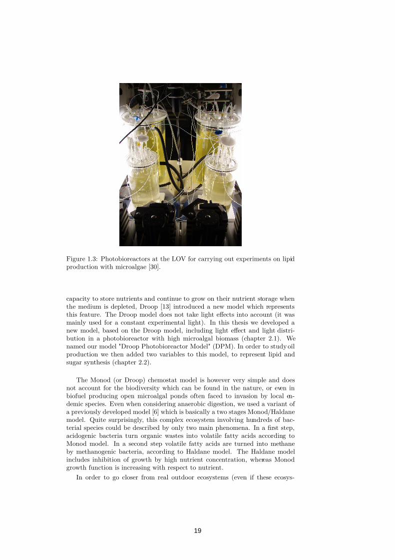
Figure 1.3: Photobioreactors at the LOV for carrying out experiments on lipidproduction with microalgae [30].
capacity to store nutrients and continue to grow on their nutrient storage whenthe medium is depleted, Droop [13] introduced a new model which representsthis feature. The Droop model does not take light effects into account (it wasmainly used for a constant experimental light). In this thesis we developed anew model, based on the Droop model, including light effect and light distri-bution in a photobioreactor with high microalgal biomass (chapter 2.1). Wenamed our model "Droop Photobioreactor Model" (DPM). In order to study oilproduction we then added two variables to this model, to represent lipid andsugar synthesis (chapter 2.2).
The Monod (or Droop) chemostat model is however very simple and doesnot account for the biodiversity which can be found in the nature, or even inbiofuel producing open microalgal ponds often faced to invasion by local en-demic species. Even when considering anaerobic digestion, we used a variant ofa previously developed model [6] which is basically a two stages Monod/Haldanemodel. Quite surprisingly, this complex ecosystem involving hundreds of bac-terial species could be described by only two main phenomena. In a first step,acidogenic bacteria turn organic wastes into volatile fatty acids according toMonod model. In a second step volatile fatty acids are turned into methaneby methanogenic bacteria, according to Haldane model. The Haldane modelincludes inhibition of growth by high nutrient concentration, whereas Monodgrowth function is increasing with respect to nutrient.
In order to go closer from real outdoor ecosystems (even if these ecosys-
19

tems are still simplified), and optimize the behaviour of exploited ecosystems,the interactions between microbial populations must be considered. One ofthe simplest interaction to be considered is competition for a limiting nutrient.Competition for a substrate between several species in an homogeneous mediumis a topic of great interest to ecologists: "when and why is coexistence possible?","can we explain the mosaic of observed spatial and temporal species distribu-tion?", "can we predict in some cases which species will win a competition andexclude all the others from the environment?".
Theoreticians predicted competitive exclusion with several competing speciesrepresented by Monod models [1, 41], and then, later on, represented by Droopmodels [25]: in both cases only one species wins the competition and excludesall the others from the chemostat. From the theoretical result, it was possible topredict the outcome of competition from parameters derived from single speciesexperiments.
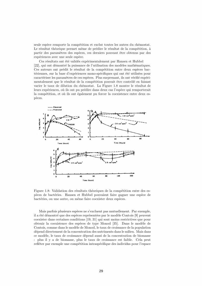
These results were experimentally validated by Hansen and Hubbel [22],which demonstrated the power of using mathematical models. These authorsexperimented the competition outcome between two bacterial species, on thebasis of single-species experiments which were used to characterize the speciesparameters. More surprisingly, they demonstrated that the outcome could betriggered by manipulating the dilution rate of the chemostat. Figure 1.8 showsthe result of their experiments, where they could predict in two cases whichspecies would win the competition, and where they could also force a coexistencebetween two species.
Figure 1.4: Validation of the theoretical competition results with bacteria.Hansen and Hubbel could make one bacteria or another win the competition,or make two species coexist.
20

But sometimes several species do not all exclude each other. For examplethe species represented by the Contois model [9] can coexist under some condi-tions [19, 31] which are less restrictive than to get coexistence from Monod typespecies [35]. In the Contois model, like in the Monod model, the populationgrowth rate depends directly on the nutrient concentration in the medium. Butin this model, the growth rate also depends on the biomass: the more biomass,the slower the population grows. This reflects e.g. intraspecific population com-petition for space (spatial heterogeneity, flocculation/deflocculation phenomena[32, 21]).
Thus with the Monod, Droop, and Contois models, we can represent threedifferent types of behaviors of the species present in microbial ecosystems. Theresult of competition is not the same for each of the models: pure Monod orDroop competition models predict competitive exclusion [41, 25], whereas pureContois competition models predict coexistence. In this thesis, we propose ageneralized result for a competition between species represented by Monod,Droop or Contois models.
One way of optimising the efficiency of an exploited microbial ecosystem is touse the competition principle to make the more efficient species win the compe-tition. This principle is a basis of the directed selection. Indeed, this techniquecan be used as an alternative to genetic engineering for identifying microorgan-isms with efficient characteristics, or for improving some species characteristics.Percival Zhang gives a review of techniques to improve a species characteristics[37]. He expresses quite clearly the interest of the "selection by competition"approach, against biotechnologist genetic rational design:
" The faith in the power of rational design relies on the belief thatour current scientific knowledge is sufficient to predict function fromstructure. But such information of structures and mechanisms is notavailable for the vast majority of enzymes. [...] An exceedingly highercell concentration of 1012 individual cells per litre and a longercultivation time (generations) allow continuous culture to become apowerful selection system for the ultra-large size of the mutant libraryeven when selective advantages are very small. "
Several examples are given [14] where competitions in specific environmentsled to the selection of population with desired traits. The review of Zelder andHauer [47] details some examples and industrial considerations.
The principle is the same as the one used in agriculture since the Neolithic toproduce bigger vegetables, by using the seeds of the biggest individuals. Alongthe course of time and generations, this led to a progressive evolution from wildplants with small fruits or seeds, to the vegetables we know today: for examplecorn with big yellow grains, which did not exist seven thousands of years ago(before the Neolithic revolution).
In the spirit of maximizing exploited microbial ecosystems performances,two approaches can be deployed. In this thesis we considered these approachesfocusing either on the individuals, or on the ecosystem.
First, the models can be used to derive control strategies which will be usedto dynamically compute the input to be applied to the ecosystem (dilution rate,influent nutrient concentrations, ...) from the knowledge of its state. Based on aPontryagin maximum principle, optimal controls are proposed which maximize
21
productivity. In this study we focus on microalgal biomass productivity opti-mization in a photobioreactor, under continuous light (chapter 3.1) or day-nightcycles (chapter 3.2). For these studies, we use our previously developed DPMmodel (chapter 2.1).
Finally, species with efficient characteristics that increase productivity mustbe chosen, and the condition to drive the ecosystem in more efficient workingmode can be found. We propose rigorous mathematical results based on themodels, to predict and control the outcome of competition in both Monod andDroop models (chapter 4.2), as well as in the anaerobic ecosystem model (chap-ter 4.3). With these results it becomes possible to change the selection criteriain the ecosystem, in order to select species with new desired characteristics thatshould help to increase productivity, both for microalgal or bacterial ecosystems.
22
Introduction
Le début du 21ème siècle est caractérisé par une prise de conscience à grandeéchelle que la façon dont l’humanité se développe actuellement n’est pas durable[28]. Le concept de l’empreinte écologique[45] a été proposé afin de comparer la demande humaine de ressources avec lacapacité écologique de la Terre à les régénérer. Il représente la surface de terrebiologiquement productive et la zone maritime nécessaires pour régénérer lesressources consommées par une population humaine et pour absorber et recy-cler les déchets correspondants. À ce jour, l’empreinte écologique moyenne d’unhabitant français est de 5 hectares globaux [15] (un hectare global représente unesurface moyenne de production sur terre), ce qui signifie que 2,5 planètes Terreseraient nécessaires pour soutenir une population de 7 milliards d’habitants vi-vant comme un habitant français moyen. Il y a deux façons de réduire notreempreinte écologique afin de laisser à nos enfants une planète avec un modèledurable dans un monde qui peut atteindre 9 milliards d’habitants avant la findu siècle. La première approche consiste à réduire radicalement nos besoinsafin d’économiser les ressources et diminuer la pollution générée. La secondeapproche, qui doit être réalisée de façon concomitante, consiste à améliorer lestechnologies que nous utilisons afin de minimiser leur impact. Cette secondeapproche, vers plus d’efficacité et moins d’impact des technologies, n’a de sensque si elle est menée en parallèle à une diminution drastique de la production,de la consommation et des déchets. Cette thèse met l’accent sur cette approchetechnologique afin de réduire l’impact du transport, qui est responsable de plusde 20 % du total des émissions de gaz à effet de serre. Afin de diminuer l’impactdes transports et de limiter l’utilisation de combustibles fossiles, des processusde production de biocarburants non-fossiles sont étudiés. Dans cette thèse nousnous sommes concentrés sur une nouvelle génération de biocarburants produitspas des organismes photosynthétiques microscopiques qui capturent l’énergiesolaire plus efficacement que les plantes terrestres.
L’énergie lumineuse du soleil est la principale source d’énergie sur Terre,dont elle soutient la vie. Les plantes sont la base même de la chaîne alimentaire,car elles sont les principaux organismes qui peuvent transformer des moléculesminérales en molécules organiques dotées d’un contenu énergétique plus élevé :ce gain d’énergie, fruit de la photosynthèse, provient de la lumière. L’énergie so-laire permet de transformer, grâce à la photosynthèse, le CO2, avec les divers élé-ments nutritifs (azote, phosphore, potassium, ...) en matière organique. À partles organismes autotrophes, tous les autres organismes (bactéries hétérotrophes,levures, animaux, ...) ont besoin de consommer de telles molécules organiqueset d’utiliser l’énergie qu’elles contiennent pour vivre. L’enzyme qui est respon-
23

sable de la fixation du C02 est la Rubisco (ribulose-1,5-bisphosphate carboxy-lase/oxygénase), qui intervient dans le cycle de Calvin [16]. Cette enzyme estl’enzyme la plus abondante sur Terre [16], et c’est aussi la protéine la plus abon-dante sur Terre, ce qui démontre le rôle crucial joué par la photosynthèse. L’idéede produire des biocarburants consiste à exploiter cette capacité des plantes àemmagasiner l’énergie lumineuse, pour récupérer ensuite l’énergie ainsi stockée.Il y a deux possibilités pour récupérer cette énergie. Soit les plantes peuvent êtrecultivées pour leur capacité à stocker l’énergie sous une forme utilisable spéci-fique (lipides, sucres) dans des organes spécialisés. L’énergie est alors récupéréesous forme d’huile qui peut être transformée en biodiesel (ou bioéthanol pourdes réserves cellulaires de sucre). Soit l’énergie peut être récupérée à partirde déchets, après que la plante a été utilisée. Dans ce cas, une communautéd’archea-bactéries et de bactéries anaérobies peut être cultivée sur les déchetsrestants et du méthane (qui est aussi un biocarburant) peut être produit. Ce sec-ond procédé peut également être combiné au traitement de déchets organiquesindustriels et ménagers, dans le but de produire de la bioénergie et de traiterdes polluants organiques en même temps.
Le phytoplancton est constitué de plantes microscopiques (microalgues etcyanobactéries) qui se trouvent dans la plupart des milieux aquatiques, que cesoit dans les océans, dans les lacs ou dans les rivières [24]. Certaines espèces peu-vent même se développer dans des environnements extrêmes, comme la glace,et d’autres peuvent être trouvées dans des geysers ou dans des lacs très acides.Plus de 30 000 espèces ont été décrites, mais il y a probablement plus d’un mil-lion d’espèces sur Terre [7]. La Figure 1.5 illustre leur très grande diversité detailles, de formes et de couleurs. Les organismes phytoplanctoniques sont sou-vent désignés par le terme "microalgues", ce qui est un abus de langage (puisqueles cyanobactéries ne sont pas, rigoureusement parlant, des microalgues), maisce terme sera utilisé dans le manuscrit.
Figure 1.5: Les microalgues peuvent être rencontrées à peu près partout sur leglobe, environ 30.000 espèces ont été référencées.
Dans les cinquante dernières années, plusieurs espèces de microalgues ontmontré des caractéristiques intéressantes pour des applications biotechnologiques: de la production de nourriture aux productions pharmaceutiques [38, 42], à lafixation de CO2 [3] et à la production de biocarburants [26, 8]. Leur haut rende-ment photosynthétique par rapport aux plantes terrestres (dont la croissance estlimitée par la disponibilité en CO2) permet de fortes productivités potentiellesen biomasse, de plusieurs ordres de grandeur plus élevées que les plantes ter-
24
restres [7]. Cette plus grande efficacité dans la récupération de l’énergie solaireest la principale raison pour laquelle plusieurs projets ont été lancés au début dece siècle. Parmi eux, le projet ANR-Shamash a pour but d’étudier et d’optimiserle potentiel de production de biocarburants à partir de microalgues. Un autreprojet ANR (Symbiose) envisage la possibilité d’utiliser des microalgues pournourrir un écosystème anaérobie, afin de produire du méthane et recycler l’azoteet le phosphore sous forme de nitrate et de phosphate, dont une nouvelle culturede microalgues pourra alors se nourrir. Ces écosystèmes anaérobies sont assezcomplexes car ils peuvent impliquer plus de 300 espèces bactériennes [11] dansdes interactions complexes. La digestion anaérobie peut être naturellement ob-servée dans les sédiments des lacs et des rivières, où des déchets sont dégradéset du méthane produit. Ce méthane est ensuite libéré dans l’atmosphère, con-tribuant ainsi au réchauffement climatique. Lorsque le processus est domestiquédans un bioréacteur (voir la figure 1.6) l’écosystème anaérobie peut à la fois pro-duire du méthane (qui sera ensuite valorisé energétiquement) et traiter les eauxusées [2].
Indépendamment de leur application directe dans les énergies renouvelables,les écosystèmes microbiens ont également un fort intérêt pour l’écologie théorique[29] : les expériences avec des écosystèmes microbiens peuvent être suivies detrès près, reproduites facilement, elles présentent une croissance rapide de lapopulation, les organismes peuvent être archivés par des procédés cryogéniques,et leurs constituants physiologiques et génétiques sont assez bien caractérisés.Ces atouts sont contrebalancés par certaines limites : l’évolution est souventrapide de telle sorte que les interactions peuvent changer avant que les chercheursaient terminé leur caractérisation. Enfin, nous sommes limités dans notre ca-pacité à extrapoler à partir de systèmes expérimentaux microbiens, vers dessystèmes plus grands et souvent plus complexes. En particulier dans cettethèse, les travaux sur le fonctionnement de la compétition ont des implica-tions conceptuelles qui pourraient également s’appliquer à des écosystèmes nonmicrobiens.
Plusieurs obstacles doivent aussi être considérés dans l’étude des écosystèmesmicrobiens : les systèmes biologiques et les environnements sont complexes, lesmesures sont souvent inexactes ou à faible fréquence d’échantillonnage, les sys-tèmes présentent souvent des non-linéarités, telles que des effets de seuil con-duisant à des réactions brusques et rapides. Pour limiter le degré de complexitéde ces systèmes, afin d’accroitre les chances de développer des modèles, il estsouvent utile de commencer par les simplifier. En 1942, Monod [36] a développéun outil pour étudier la dynamique microbienne : le chémostat. C’est un récip-ient dans lequel on injecte continument du milieu de croissance. Pour garderun volume constant dans le récipient, un mélange de nutriments et de micro-organismes est évacué à la même vitesse que le débit d’entrée. Un tel systèmepermet d’isoler les micro-organismes des variations environnementales (lumière,température, ....) et ainsi de contrôler avec précision les conditions de croissance.Il permet également de surveiller précisément la croissance des organismes, grâceà des capteurs dédiés. Au cours de cette thèse, des expériences ont été faitesdans les photobioréacteurs continus (cultures de microalgues en chémostats) duLOV (Laboratoire d’Océanographie de Villefranche-sur-Mer), que l’on peut voirà la Figure 1.7. Les éléments nutritifs, la lumière, la température et le pH étaientmesurés en ligne et pour certains d’entre eux, régulés. La plupart de ces expéri-
25

Figure 1.6: Fermenteur anaérobie du Laboratoire de Biotechnologie del’Environnement, INRA, Narbonne.
26
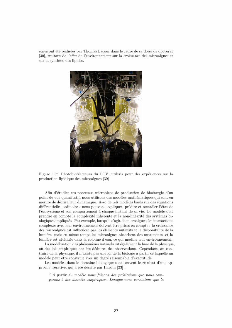
ences ont été réalisées par Thomas Lacour dans le cadre de sa thèse de doctorat[30], traitant de l’effet de l’environnement sur la croissance des microalgues etsur la synthèse des lipides.
Figure 1.7: Photobioréacteurs du LOV, utilisés pour des expériences sur laproduction lipidique des microalgues [30]
Afin d’étudier ces processus microbiens de production de bioénergie d’unpoint de vue quantitatif, nous utilisons des modèles mathématiques qui sont enmesure de décrire leur dynamique. Avec de tels modèles basés sur des équationsdifférentielles ordinaires, nous pouvons expliquer, prédire et contrôler l’état del’écosystème et son comportement à chaque instant de sa vie. Le modèle doitprendre en compte la complexité inhérente et la non-linéarité des systèmes bi-ologiques impliqués. Par exemple, lorsqu’il s’agit de microalgues, les interactionscomplexes avec leur environnement doivent être prises en compte : la croissancedes microalgues est influencée par les éléments nutritifs et la disponibilité de lalumière, mais en même temps les microalgues absorbent des nutriments, et lalumière est atténuée dans la colonne d’eau, ce qui modifie leur environnement.
La modélisation des phénomènes naturels est également la base de la physique,où des lois empiriques ont été déduites des observations. Cependant, au con-traire de la physique, il n’existe pas une loi de la biologie à partir de laquelle unmodèle peut être construit avec un degré raisonnable d’exactitude.
Les modèles dans le domaine biologique sont souvent le résultat d’une ap-proche itérative, qui a été décrite par Hardin [23] :
" À partir du modèle nous faisons des prédictions que nous com-parons à des données empiriques. Lorsque nous constatons que la
27
prédiction n’est pas vérifiée, nous modifions alors le modèle. Il n’y apas de règle ni de procédure pour nous dire quels éléments du modèledevraient être abandonnés ou modifiés. (...). L’ esthétique joue unrôle dans cette décision. "
Monod a développé un modèle pionnier, où le taux de croissance bactérienest directement lié à la disponibilité en éléments nutritifs dans le milieu. Commele phytoplancton a une capacité à stocker des éléments nutritifs et à continuer àcroître sur ses stocks d’éléments nutritifs lorsque le milieu est appauvri, Droop[13] a introduit un nouveau modèle qui représente ce processus. Le modèle deDroop ne prend pas en compte les effets de la lumière (il a été principalementutilisé pour une lumière expérimentale constante). Dans cette thèse nous avonsdéveloppé un nouveau modèle, basé sur le modèle de Droop, comprenant leseffets de la lumière et de la distribution de la lumière dans un photobioréac-teur à forte biomasse de microalgues (chapitre 2.1). Nous avons nommé notremodèle "Droop Photobioreactor Model" (DPM). Afin d’étudier la productiond’huile nous avons ensuite ajouté deux variables à ce modèle, pour représenterla synthèse des lipides et du sucre (chapitre 2.2).
Lorsque nous avons considéré la digestion anaérobie, nous avons utilisé unevariante d’un modèle précédemment développé [6] qui est essentiellement unmodèle Monod / Haldane à deux étapes. De manière étonnante, cet écosystèmecomplexe impliquant des centaines d’espèces de bactéries peut être décrit parseulement deux réactions principales. Dans un premier temps, des bactériesacidogènes transforment les déchets organiques en acides gras volatils selon lemodèle de Monod. Dans une deuxième étape ces acides gras volatils sont trans-formés en méthane par des bactéries méthanogènes, selon le modèle de Haldane.Le modèle de Haldane représente une inhibition de la croissance par les concen-trations élevées en nutriments, alors que la fonction de croissance de Monodaugmente toujours avec la concentration en éléments nutritifs.
Ce dernier modèle, ainsi que les modèles de chémostat de Monod et deDroop, sont très simples et ne tiennent pas compte de la diversité biologiquequi se trouve dans la nature, ou même dans les étangs ouverts de culture de mi-croalgues, qui sont souvent confrontés à l’invasion par des espèces compétitriceslocales.
Pour se rapprocher des écosystèmes réels, en plein air (même si ces écosys-tèmes sont encore simplifiés), et optimiser le comportement de ces écosystèmes,les interactions entre différentes populations microbiennes doivent être consid-érées. L’une des interactions les plus simples à prendre en compte est la com-pétition pour un élément nutritif limitant. La compétition pour un substratentre plusieurs espèces dans un milieu homogène est un sujet de grand intérêtpour les écologistes : "quand et pourquoi des situations de coexistence sont-ellespossibles?", "Peut-on expliquer les mosaïques spatiales et temporelles de distri-bution des espèces?", "Peut-on prévoir dans certains cas quelle espèce gagne lacompétition et va ainsi exclure toutes les autres de l’environnement?".
Dans le cas d’une compétition entre plusieurs espèces représentées par desmodèles de Monod, la théorie prédit l’exclusion compétitive.[1, 41]. Ce même résultat a ensuite été étendu à une compétition entre desespèces représentées par des modèles de Droop [25] : dans les deux cas une
28
seule espèce remporte la compétition et exclut toutes les autres du chémostat.Le résultat théorique permet même de prédire le résultat de la compétition, àpartir des paramètres des espèces, ces derniers pouvant être obtenus par desexpériences avec une seule espèce.
Ces résultats ont été validés expérimentalement par Hansen et Hubbel[22], qui ont démontré la puissance de l’utilisation des modèles mathématiques.Ces auteurs ont prédit le résultat de la compétition entre deux espèces bac-tériennes, sur la base d’expériences mono-spécifiques qui ont été utilisées pourcaractériser les paramètres de ces espèces. Plus surprenant, ils ont vérifié expéri-mentalement que le résultat de la compétition pouvait être contrôlé en faisantvarier le taux de dilution du chémostat. La Figure 1.8 montre le résultat deleurs expériences, où ils ont pu prédire dans deux cas l’espèce qui remporteraitla compétition, et où ils ont également pu forcer la coexistence entre deux es-pèces.
Figure 1.8: Validation des résultats théoriques de la compétition entre des es-pèces de bactéries. Hansen et Hubbel pouvaient faire gagner une espèce debactéries, ou une autre, ou même faire coexister deux espèces.
Mais parfois plusieurs espèces ne s’excluent pas mutuellement. Par exemple,il a été démontré que des espèces représentées par le modèle Contois [9] peuventcoexister dans certaines conditions [19, 31] qui sont moins restrictives que pourobtenir la coexistence des espèces de type Monod [35]. Dans le modèle deContois, comme dans le modèle de Monod, le taux de croissance de la populationdépend directement de la concentration des nutriments dans le milieu. Mais dansce modèle, le taux de croissance dépend aussi de la concentration de biomasse: plus il y a de biomasse, plus le taux de croissance est faible. Cela peutrefléter par exemple une compétition intraspécifique des individus pour l’espace
29

(hétérogénéité spatiale, phénomènes de floculation / défloculation [32, 21]).Ainsi, avec les modèles de Monod, Droop, et Contois, on peut représenter
trois types de comportements différents d’espèces présentes dans les écosystèmesmicrobiens. Le résultat de la compétition n’est pas la même pour chacun desmodèles : dans les modèles de compétition pure entre des espèces représentéespar le modèle de Monod ou celui de Droop , la théorie prédit l’exclusion com-pétitive [41, 25], tandis que les modèles de compétition pure entre des espècesreprésentées par le modèle Contois prédisent la coexistence. Dans cette thèse,nous proposons une généralisation de ces résultats, en mettant en compétitionmixte des espèces représentées par des modèles de Monod, Droop et Contois.
Une façon d’optimiser l’efficacité d’un écosystème microbien est d’utiliserle principe de compétition pour faire remporter la compétition à l’espèce laplus efficace. C’est le principe de base de la Sélection Dirigée. Cette tech-nique peut être utilisée comme une alternative au génie génétique, pour identi-fier les micro-organismes ayant des caractéristiques efficaces, ou pour améliorercertaines caractéristiques d’une population donnée. Percival Zhang donne unevue d’ensemble des techniques permettant d’améliorer les caractéristiques d’unepopulation [37]. Il exprime très clairement l’intérêt de l’approche de "sélectionpar compétition", par rapport au "genetic rational design" des biotechnologistes:
" La foi dans la puissance du "rational design" repose sur la con-viction que nos connaissances scientifiques actuelles sont suffisantespour prédire la fonction à partir de la structure. Mais de telles infor-mations sur les structures et les mécanismes ne sont pas disponiblespour la grande majorité des enzymes. [...] Une concentration cellu-laire extrêmement élevée d’environ 1012 cellules par litre et un longtemps de culture (de l’ordre de dizaines ou centaines de générations)permettent à la culture continue de devenir un système de sélectionpuissant dans la bibliothèque immense des mutants, même lorsqueles avantages sélectifs sont infimes. "
Plusieurs exemples sont donnés [14] où des compétitions dans des environ-nements spécifiques ont conduit à la sélection d’une population ayant des car-actéristiques souhaitées. La review de Zelder et Hauer [47] détaille quelquesexemples et donne des considérations industrielles.
Le principe est le même que celui utilisé dans l’agriculture depuis le Néolithiquepour produire de plus gros légumes, en utilisant les graines des plus gros in-dividus. Au fil du temps et des générations, cela a conduit à une évolutionprogressive à partir de plantes sauvages à petits fruits ou graines, jusqu’auxlégumes que nous connaissons aujourd’hui : par exemple le maïs avec de grosgrains jaunes, qui n’existait pas il y a sept milliers d’années (avant la Révolutionnéolithique).
Dans l’esprit de maximiser les performances des écosystèmes microbiens con-trôlés, deux approches peuvent être déployées. Dans cette thèse, nous avonsétudié ces deux approches, centrées soit sur les individus, soit sur l’écosystème.
D’abord, les modèles peuvent être utilisés pour déterminer des stratégies decontrôle qui seront utilisées pour calculer à chaque instant l’entrée à appliquerà l’écosystème (taux de dilution, concentration en nutriments de l’influent, ...)à partir de la connaissance de son état. Basé sur le principe du maximum de
30

Pontryagin, nous proposons des stratégies de contrôle optimales qui permettentde maximiser la productivité. Dans cette étude, nous nous concentrons surl’optimisation de la productivité de la biomasse de microalgues dans un photo-bioréacteur, sous une lumière continue (chapitre 3.1) ou sous des cycles jour-nuit(chapitre 3.2). Pour ces études, nous utilisons notre modèle "DPM" développéantérieurement (chapitre 2.1).
Enfin, les espèces ayant des caractéristiques efficaces qui augmentent la pro-ductivité doivent être choisies. Nous proposons des résultats mathématiquesrigoureux basés sur les modèles, pour prévoir et contrôler le résultat de la com-pétition dans les modèles de Monod et de Droop (chapitre 4.2), ainsi que dansle modèle d’écosystème anaérobie (chapitre 4.3). Avec ces résultats, il devientpossible de changer les critères de sélection dans l’écosystème, afin de sélection-ner des espèces possédant de nouvelles caractéristiques souhaitées, qui devraientcontribuer à accroître la productivité, tant pour les écosystèmes de microalguesque pour ceux de bactéries.
31

32
Chapter 2
Photobioreactor modelling
A first approach for studying microorganisms consists in growing them in "batch",i.e. with a predefined quantity of nutrients that they will consume. When thenutrients are depleted, the population stops growing. In general, in the twobioreactor types that we will consider (photobioreactor and anaerobic digester),only one nutrient will be limiting, and we denote this nutrient’s concentration s
(for "substrate"). To get closer to the conditions of natural environments wherewater and nutrients are renewed (sea, lakes, etc.), researchers began to changethe nutritive medium after periodic time intervals [17]. This approach was im-proved by changing part of the medium continuously, which is achieved in achemostat. Water continuously comes in, enriched with nutrients (with con-centration sin), and goes out together with microorganisms and the remainingnutrients. The flow of water leads to a dilution rate denoted D, which corre-sponds to the proportion of medium renewed each day. The main biologicalphenomena occurring in the chemostat are substrate absorption (ρ will be theabsorption rate per population unit) and population growth, whose rate willbedenoted µ. Thus, with x the microorganisms biomass concentration (e.g. ingrams of carbon per liter), a chemostat model can be written:
nutrients concentration change = nutrients input− nutrients output−nutrients absorption
microalgal biomass change = growth−microalgae going out of the chemostat
(2.1)This model can also be written with mathematical symbols:
{
s = Dsin − Ds − ρ(.)xx = µ(.)x − Dx
(2.2)
This general chemostat model is presented in Figure 2.1.Many variants of this chemostat model were developed, with different factors
affecting absorption and growth rates. Monod model [36] states that the growthrate is proportional to the absorption rate :
µ(.) = kρ(.)
it means that microorganisms need a fixed amount of substrate for building onebiomass unit. In this model also, the growth rate is a function of the outputsubstrate concentration s.
33
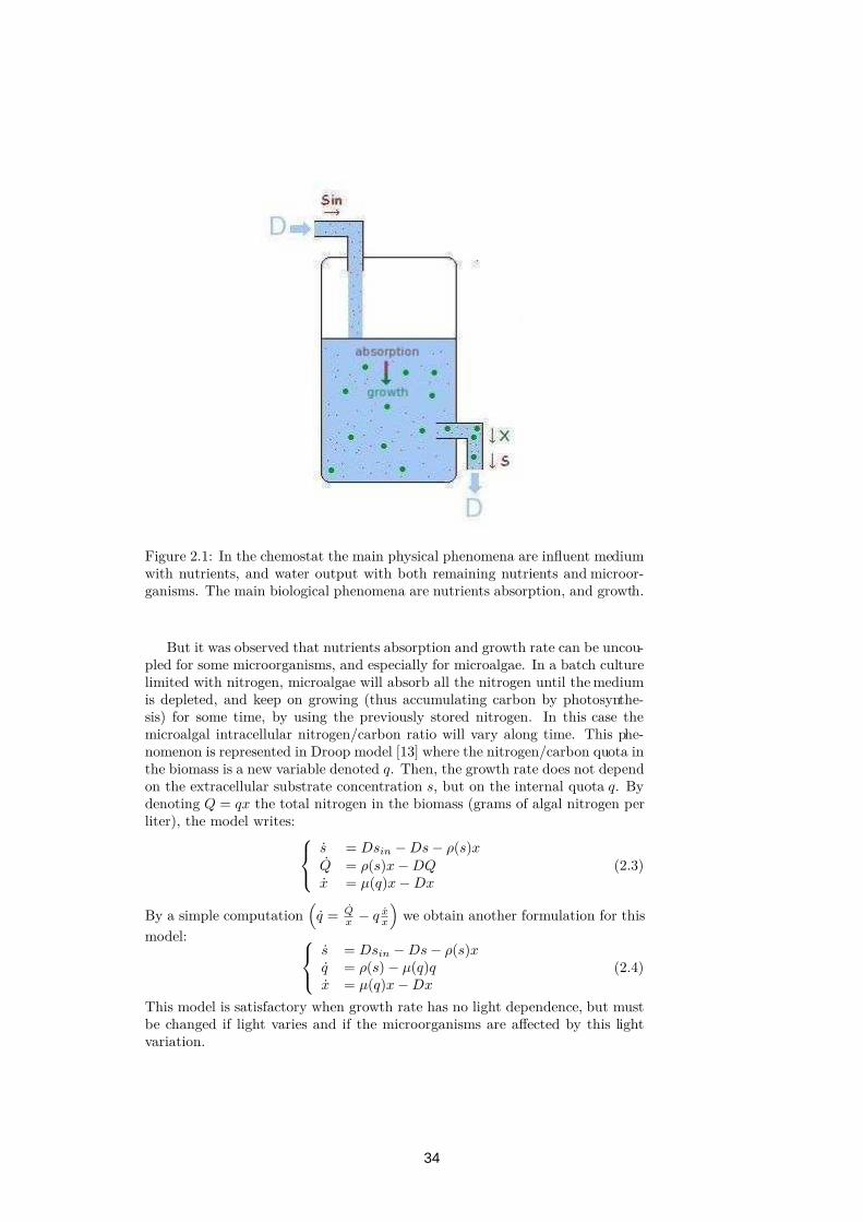
Figure 2.1: In the chemostat the main physical phenomena are influent mediumwith nutrients, and water output with both remaining nutrients and microor-ganisms. The main biological phenomena are nutrients absorption, and growth.
But it was observed that nutrients absorption and growth rate can be uncou-pled for some microorganisms, and especially for microalgae. In a batch culturelimited with nitrogen, microalgae will absorb all the nitrogen until the mediumis depleted, and keep on growing (thus accumulating carbon by photosynthe-sis) for some time, by using the previously stored nitrogen. In this case themicroalgal intracellular nitrogen/carbon ratio will vary along time. This phe-nomenon is represented in Droop model [13] where the nitrogen/carbon quota inthe biomass is a new variable denoted q. Then, the growth rate does not dependon the extracellular substrate concentration s, but on the internal quota q. Bydenoting Q = qx the total nitrogen in the biomass (grams of algal nitrogen perliter), the model writes:
s = Dsin − Ds − ρ(s)xQ = ρ(s)x − DQ
x = µ(q)x − Dx
(2.3)
By a simple computation(
q = Q
x− q x
x
)
we obtain another formulation for this
model:
s = Dsin − Ds − ρ(s)xq = ρ(s) − µ(q)qx = µ(q)x − Dx
(2.4)
This model is satisfactory when growth rate has no light dependence, but mustbe changed if light varies and if the microorganisms are affected by this lightvariation.
34

In order to produce energy from microalgae, since the light conversion yieldis lower than 20% [7], electric energy cannot reasonably be used as a source oflight. Thus, the sun is the only sustainable energy source to support microalgalgrowth. Since light varies along the day-night cycle, it will affect photosynthesisand thus microalgal growth. More precisely, when considering a photobioreactoror a raceway to grow outdoor microalgae, the following aspects must be takeninto account:
• when biomass is high the light is attenuated by pigments (mainly chloro-phyll);
• under this condition, respiration is not negligible and must be considered;
• high light intensities lead to a photoinhibition which decreases the growthrate;
• Microalgae photoacclimate to light intensity: they adapt their chlorophyllto the incident flux of photons. As a consequence, the chlorophyll/carbonratio varies with light intensity in the photobioreactor, and is linked tothe nitrogen/carbon ratio.
For the optimization works presented in this thesis (chapter 3), we neededa model that would take all these phenomena into account, while being simpleenough to be validable, identifiable, and to allow a mathematical analysis. Thephotobioreactor models encountered in literature did not meet these criteria[40, 39], so we had to build our own model. In particular, the models developedin [34, 5] were too complex for identification and mathematical analysis. In thefollowing we present a new photobioreactor model, based on Droop’s formu-lation, and called Droop Photobioreactor Model (DPM). It contains the mainDroop’s ingredients, as well as the light effect, auto shading by the microalgalpopulation and photoacclimation mechanisms.
Finally, we need a lipid synthesis model for assessing lipid productivity.This model, developped in cooperation with the biologists of the Laboratoired’Océanographie de Villefranche-sur-mer, represents lipid and sugar synthesis,as well as a functionnal carbon pool. Its singularity is that lipids are accumu-lated during nitrate stresses (for example in the final stationnary phase of abatch culture), whereas the lipid/carbon quota decreases under nitrate limita-tion in a continuous culture at equilibrium. The sugar/carbon quota at equilib-rium increases with increasing nitrate concentration in the medium. Finally, thefunctionnal carbon pool is constitued of all the remaining carbon. The variablesof this model can be added to the Droop model, as presented in the paper, orto the DPM model.
35

Modelling planar photobioreactors in nitrogen limited
conditions
Olivier Bernarda,∗, Francis Maireta, Pierre Mascia, Antoine Sciandrab
aCOMORE-INRIA, BP93, 06902 Sophia-Antipolis Cedex, FrancebLOV, UMR 7093, Station Zoologique, B.P. 28 06234, Villefranche-sur-mer, France
Abstract
Oleaginous microalgae are seen as a potential major biofuel producer in the futuresince, under conditions of nitrogen deprivation, they can contain high amountsof lipids. In order to optimize productivity in a microalgal production system(including open raceways and closed photobioreactors), we develop a new modelto predict biomass dynamics in conditions of nitrogen limitation and light gra-dient. On the basis of the Droop model, we represent light influence, and thenwe relate the chlorophyll content to the nitrogen cell quota, for a given photoac-climation light. In a second step, we compute the light distribution thanks toa Beer-Lambert law. It results in a model where biology (microalgal growth innitrogen limited conditions) and physics (radiative transfer) are strongly coupled.Dynamical photoacclimation to light variation is the key biological phenomenonthat couples these two aspects. The mathematical complexity is kept at a minimallevel so that the model calibration is rather straightforward. The model is assessedwith experimental data of Isochrysis galbana under light/dark cycles. This modelshows that, when averaged along photobioreactor depth, the photoinhibition fea-ture of a microalgal species may apparently disappear while photoinhibition re-duces overall productivity. The proposed model can be the basis for research ofworking conditions which optimize biomass or lipid productivity.
Key words: Microalgae, modelling, photoacclimation, photoinhibition, nitrogenlimitation, photobioreactor, biofuel
Autotrophic microalgae and cyanobacteria use photons as energy source to fixcarbon dioxide (CO2). These microorganisms have recently received a specific at-
∗Olivier BernardBP93, 06902 Sophia-Antipolis, FranceTel:+33 492 387 785Fax:+33 492 387 858Email: [email protected]
Preprint submitted to Biotech. Bioeng. August 30, 2010
36
tention in the framework of renewable energy. Their high actual photosyntheticyield compared to terrestrial plants (whose growth is limited by CO2 availability)leads to large potential algal biomass productions of several tens of tons perhectareand per year (Chisti, 2007). After a nitrogen starvation, some oleaginous microal-gal species can reach a very high lipid content (up to 80% of dry weight (Metting,1996)). These possibilities have led some authors to consider that microalgae couldbe one of the main biofuel sources in the future (Huntley and Redalje, 2007; Chisti,2007). Lipid can be extracted from the biomass to produce biodiesel (Huntley andRedalje, 2007), while anaerobic digestion of the residual biomass (Chisti, 2007;Sialve et al., 2009) can generate methane.
On top of this, the ability of microalgae to fix CO2 in a controlled way has re-cently involved them in the race for mitigation systems (Benemann, 1997; Olaizola,2003). Thus microalgal biofuel production systems could be associated to indus-trial power plants with a high CO2 production. In the same spirit, microalgae couldbe used to consume inorganic nitrogen and phosphorus, and thus avoid expensivewastewater treatment plants.
These advantages put microalgae in a good position for renewable energy pro-duction at large scale (Chisti, 2007). This means that, in the coming years, theremight be industrial plants to produce microalgae dedicated to energy production.However, the culture of algae is not straightforward and suffers from many limi-tations (Pulz, 2001; Carvalho et al., 2006). In this article we will consider planarmicroalgal production systems including open raceways and closed photobioreac-tors, which will be called photobioreactors (PBR) for sake of brevity. We willassume that microalgal growth is not limited by inorganic carbon availability, andthus that light and inorganic nitrogen are driving microalgal kinetics.
Extensive microalgae production in PBR is a complex process that should bestrongly monitored and optimized through on-line control algorithms. In this ob-jective, a model is a powerful tool to support an automatic control strategy. SeveralPBR models exist, especially to deal with light transfer properties in the culturemedium (Suh and Lee, 2003; Pottier et al., 2005; Franco-Lara et al., 2006), butnone of them considered the microalgal kinetics in condition of nutrient limitationand none of them deal with photoacclimation.
In the specific case of biodiesel production, nitrogen starvation is known to in-crease the lipid content of phytoplankton (Spoehr and Milner, 1949; Rodolfi et al.,2009; Pruvost et al., 2009). But, it also strongly affects the pigment composi-tion and concentration (Turpin, 1991; Geider et al., 1996; Sciandra et al., 1997;Stramski et al., 2002; Geider et al., 1998), which modifies the radiative transferproperties in the culture medium (Stramski et al., 2002). The objective of ourmodelling approach is to propose a new model that can predict the behaviour of aPBR characterized by varying irradiance gradient and nitrogen availability, which
2
37

are both conditions susceptible of modifying pigment concentrations.The targeted model must keep a level of complexity compatible with the re-
quested mathematical analyses necessary for deriving optimal control algorithms.We will thus consider the simplest model that contains the elements to reproduceboth the ability of microalgae to adapt their pigments to a given irradiance (pho-toacclimation) (Anning et al., 2000; MacIntyre et al., 2002) and the reduction ofthe cell pigment contents in case of nitrogen limitation (Laws and Bannister, 1980;Sciandra et al., 2000). The basis of our development is Droop model (Droop, 1968,1983) which has been deeply investigated (Lange and Oyarzun, 1992; Bernard andGouzé, 1995, 2002; Vatcheva et al., 2006) and proved to accurately reproduce situ-ations of nitrogen limitations (Droop, 1983; Sciandra and Ramani, 1994; Bernardand Gouzé, 1999) in constant light conditions. A link between cellular nitrogenand chlorophyll will then be introduced, so that, for a planar geometry, a simplifiedirradiance distribution model within the reactor can be proposed.
The paper is organized as follows. In a first part, we recall Droop model. Thenwe introduce the light influence in this model. In a third part we propose a modelto infer chlorophyll concentrations. Finally the radiative transfer is examined, andthe photoacclimation equation is proposed. The model is then validated usingdata from Isochrysis galbana light/dark cultures.
1. Recall and presentation of Droop model
Droop model, initially established to represent the effect of B12 Vitamin in-ternal quota on the growth rate of phytoplankton (Droop, 1968), has been shownappropriate to represent also the effect of macronutrients, such as nitrogen, ongrowth rate (Droop, 1983). Contrarily to Monod model in which the growth isrelated to the limiting substrate external concentration (s), Droop model considersthat nutrient uptake and growth are uncoupled processes. Growth of the biomass(expressed in carbon and denoted x) is thus assumed to be related to the nitro-gen cell concentration for nitrogen limited microalgae. The intracellular nitrogencell concentration, or quota (q), is defined by the amount of limiting element perbiomass unit. The model equations, in a chemostat with dilution rate D andinfluent inorganic nitrogen (nitrate or ammonium) concentration sin writes:
s = Dsin − ρ(s)x−Ds
q = ρ(s)− µ(q)q
x = µ(q)x−Dx
(1)
In this model the absorption rate ρ(s) and the growth rate µ(q) are generally
3
38

taken as Michaelis-Menten and Droop functions:
ρ(s) = ρms
s+Ks
µ(q) = µ(1− Q0
q)
(2)
where Ks is the half saturation constant for substrate uptake, associated withthe maximum uptake rate ρm. Parameter µ is defined as the growth rate athypothetical infinite quota, while Q0 is the minimal nitrogen cell quota for whichno algal growth can take place. This model is more accurate than Monod modelfor algal growth modelling (Vatcheva et al., 2006), but it is more complex and hasbeen less studied from a mathematical point of view. Droop model is howeversufficiently simple to allow a detailed mathematical analysis (Lange and Oyarzun,1992; Bernard and Gouzé, 1995, 2002; Vatcheva et al., 2006), and link the modelparameters to measurable quantities.
Property 1. Droop model guarantees that internal quota stays between two bounds:
Q0 ≤ q ≤ Qm (3)
WhereQm = Q0 +
ρmµ
(4)
represents the maximum cell quota obtained in conditions of non limiting nutrient.The growth rate is also bounded :
0 ≤ µ(q) ≤ µm =ρm
Q0µ+ ρmµ (5)
where µm is the maximum growth rate reached in non limiting conditions.
Proof: See e.g. (Bernard and Gouzé, 1995).As a corollary of this property, most of Droop model parameters can be straightfor-wardly identified from the measurements of the internal quota during nonlimitedgrowth (for which µ(Qm) = µm) and at the end of a batch phase, when growthrate becomes zero for a minimal value of the quota q = Q0. The internal quota innonlimited growth conditions (when q = Qm) together with the maximum growthrate provides then the values of µ and ρm:
ρm = µmQm and µ = µmQm
Qm −Q0
(6)
Parameter Ks can be deduced (together with another estimate of ρm) froma batch experiment where the disappearance of inorganic nitrogen is measuredtogether with algal biomass.
4
39
Droop model has been widely validated (Droop, 1983; Sciandra and Ramani,1994; Bernard and Gouzé, 1999; Vatcheva et al., 2006). However, it cannot directlybe used in the case of PBR for two main reasons:
• In its rough form it does not include the irradiance effect.
• It does not account for light gradient due to the cell density in the PBR
2. Improvement of Droop model to deal with light limitation
2.1. Inorganic carbon uptake rate
Droop model does not take irradiance into account. Including light is how-ever not straightforward. A first approach consists in representing the light effectthrough µ = µ(I) (Han, 2001):
µ(q, I) = µ(I)(1− Q0
q) (7)
where we use, depending on the species, two possible expressions for µ(I). For thespecies that do not photoinhibit, we use a simple kinetic (Han, 2001):
µa(I) = µaI
I +KasI(8)
Parameter KasI refers to the half saturation coefficient with respect to light, andµa is the hypothetical maximal growth rate without photoinhibition.
This simple expression will be used as a first approximation for species whosephotoinhibition is limited. With this simplified point of view the computationstays tractable and it leads to the model denoted (Sa) . However, we will alsoconsider the more complex model of Eilers and Peeters (1988, 1993):
µb(I) = µI
I +KbsI + I2
KbiI
(9)
Here an inhibition coefficient KbiI is considered, together with parameter KbsI ,
they define the light intensity Iopt =√
KbsIKbiI for which µb(I) is maximal. Pa-
rameter µb is the hypothetical growth rate at non limiting irradiance and withoutinhibition.
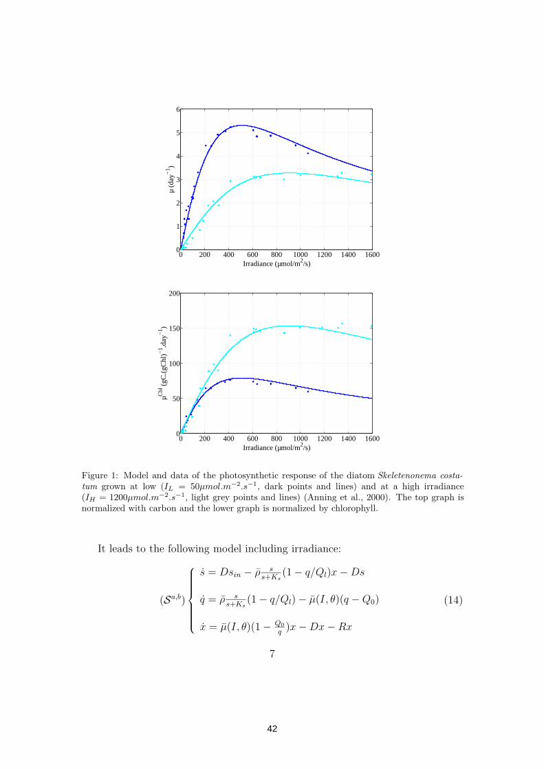
It is well known that, for eukaryotic microalgae, the initial slope of a photo-synthesis irradiance (P-I) curve normalized with Chl a does not depend on thelight at which cells have been photoadapted (MacIntyre et al., 2002). This can beobserved on Figure 1 for the diatom Skeletenonema costatum. In mathematicalterms, this property constraints the model in the sense that the parameter αChl,
5
40

defined by the initial slope of the curve µ(I)/θ has to be independent of the ratioθ = Chl/x. Parameter αChl can be computed from equation (9):
αChl =µ
θKbsI(10)
To ensure that αChl is a constant, it implies that KbsI has to be computed from θas follows:
KbsI = K∗sI/θ (11)
Indeed, with this expression, the initial slope of the inorganic carbon uptake ratenormalized by chlorophyll is constant: αChl = µ
K∗sI
A comparison of model given by equation (9) with the data of Anning et al.(2000) with the diatom Skeletonema costatum is presented figure 1. The datashows experiments where the cells have been photoadapted at a low irradiance(IL = 50µmol.m−2.s−1) and at a high irradiance (IH = 1200µmol.m−2.s−1). Model(9) together with equation (11) turns out to accurately represent these data.
When considering equation (9), we denote (Sb) the corresponding model.
2.2. Inorganic nitrogen uptake rate
When including light effect in the growth rate, the maximum inorganic nitrogenuptake rate must be adapted to limit cell quota increase. Indeed, with Droopmodel, when keeping a constant maximum uptake rate, equation 4 becomes:
Qm(I) = Q0 +ρmµ(I)
(12)
Then, during night periods, µ(0) = 0 and thus equation (12) would lead to aninfinite maximal quota. Indeed, with such a formulation no growth occurs atnight, so that the substrate can be indefinitely taken up into the cell without beingconsumed for growth. If an increase of the maximum cell quota in the absence oflight is possible (Laws and Bannister, 1980), obviously it cannot become infinite.
We impose therefore, in line with Geider et al. (1998), that the uptake ratestops as cells become replete:
ρ(s, q) = ρs
s+Ks(1− q/Ql) (13)
where parameter Ql > Q0 is the maximal internal quota in dark conditions.
2.3. Model synthesis
Finally we consider a respiration term. As in Geider et al. (1998), we assumethat the rate of nitrogen loss (due both to mortality and excretion) is the samethan the respiration rate.
6
41
0 200 400 600 800 1000 1200 1400 16000
1
2
3
4
5
6
µ (
day−
1 )
Irradiance (µmol/m2/s)
0 200 400 600 800 1000 1200 1400 16000
50
100
150
200
Irradiance (µmol/m2/s)
µChl
(gC
.(gC
hl)−
1 .day
−1 )
Figure 1: Model and data of the photosynthetic response of the diatom Skeletenonema costa-
tum grown at low (IL = 50µmol.m−2.s−1, dark points and lines) and at a high irradiance(IH = 1200µmol.m−2.s−1, light grey points and lines) (Anning et al., 2000). The top graph isnormalized with carbon and the lower graph is normalized by chlorophyll.
It leads to the following model including irradiance:
(Sa,b)
s = Dsin − ρ ss+Ks
(1− q/Ql)x−Ds
q = ρ ss+Ks
(1− q/Ql)− µ(I, θ)(q −Q0)
x = µ(I, θ)(1− Q0
q)x−Dx−Rx
(14)
7
42
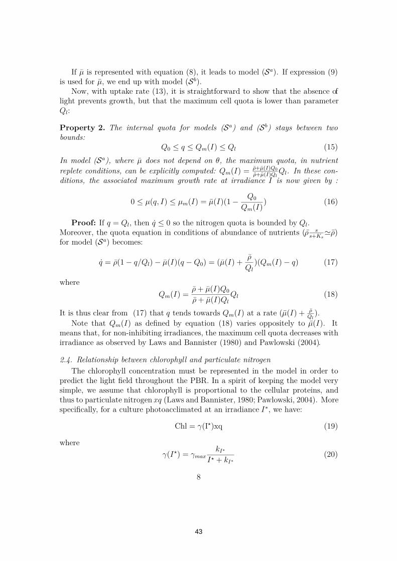
If µ is represented with equation (8), it leads to model (Sa). If expression (9)is used for µ, we end up with model (Sb).
Now, with uptake rate (13), it is straightforward to show that the absence oflight prevents growth, but that the maximum cell quota is lower than parameterQl:
Property 2. The internal quota for models (Sa) and (Sb) stays between twobounds:
Q0 ≤ q ≤ Qm(I) ≤ Ql (15)
In model (Sa), where µ does not depend on θ, the maximum quota, in nutrient
replete conditions, can be explicitly computed: Qm(I) = ρ+µ(I)Q0
ρ+µ(I)QlQl. In these con-
ditions, the associated maximum growth rate at irradiance I is now given by :
0 ≤ µ(q, I) ≤ µm(I) = µ(I)(1− Q0
Qm(I)) (16)
Proof: If q = Ql, then q ≤ 0 so the nitrogen quota is bounded by Ql.Moreover, the quota equation in conditions of abundance of nutrients (ρ s
s+Ks≃ρ)
for model (Sa) becomes:
q = ρ(1− q/Ql)− µ(I)(q −Q0) = (µ(I) +ρ
Ql)(Qm(I)− q) (17)
where
Qm(I) =ρ+ µ(I)Q0
ρ+ µ(I)QlQl (18)
It is thus clear from (17) that q tends towards Qm(I) at a rate (µ(I) + ρQl
).
Note that Qm(I) as defined by equation (18) varies oppositely to µ(I). Itmeans that, for non-inhibiting irradiances, the maximum cell quota decreases withirradiance as observed by Laws and Bannister (1980) and Pawlowski (2004).
2.4. Relationship between chlorophyll and particulate nitrogen
The chlorophyll concentration must be represented in the model in order topredict the light field throughout the PBR. In a spirit of keeping the model verysimple, we assume that chlorophyll is proportional to the cellular proteins, andthus to particulate nitrogen xq (Laws and Bannister, 1980; Pawlowski, 2004). Morespecifically, for a culture photoacclimated at an irradiance I∗, we have:
Chl = γ(I⋆)xq (19)
where
γ(I⋆) = γmaxkI∗
I⋆ + kI∗(20)
8
43
0 50 100 150 200 2500
0.02
0.04
0.06
0.08
0.1
0.12
Irradiance (µmol.m -2.s-1)
Chl
/N (
g/g)
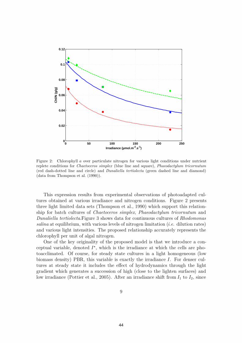
Figure 2: Chlorophyll a over particulate nitrogen for various light conditions under nutrientreplete conditions for Chaetoceros simplex (blue line and square), Phaeodactylum tricornutum
(red dash-dotted line and circle) and Dunaliella tertiolecta (green dashed line and diamond)(data from Thompson et al. (1990)).
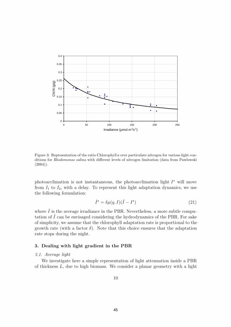
This expression results from experimental observations of photoadapted cul-tures obtained at various irradiance and nitrogen conditions. Figure 2 presentsthree light limited data sets (Thompson et al., 1990) which support this relation-ship for batch cultures of Chaetoceros simplex, Phaeodactylum tricornutum andDunaliella tertiolecta.Figure 3 shows data for continuous cultures of Rhodomonassalina at equilibrium, with various levels of nitrogen limitation (i.e. dilution rates)and various light intensities. The proposed relationship accurately represents thechlorophyll per unit of algal nitrogen.
One of the key originality of the proposed model is that we introduce a con-ceptual variable, denoted I⋆, which is the irradiance at which the cells are pho-toacclimated. Of course, for steady state cultures in a light homogeneous (lowbiomass density) PBR, this variable is exactly the irradiance I. For denser cul-tures at steady state it includes the effect of hydrodynamics through the lightgradient which generates a succession of high (close to the lighten surfaces) andlow irradiance (Pottier et al., 2005). After an irradiance shift from I1 to I2, since
9
44
0
0.05
0.1
0.15
0.2
0.25
0.3
0.35
0.4
0 50 100 150 200 250
Irradiance (µmol.m .s )
Chl
:N (
g/g)
-1-2
Figure 3: Representation of the ratio Chlorophylla over particulate nitrogen for various light con-ditions for Rhodomonas salina with different levels of nitrogen limitation (data from Pawlowski(2004)).
photoacclimation is not instantaneous, the photoacclimation light I⋆ will movefrom I1 to I2, with a delay. To represent this light adaptation dynamics, we usethe following formulation:
I⋆ = δµ(q, I)(I − I⋆) (21)
where I is the average irradiance in the PBR. Nevertheless, a more subtle compu-tation of I can be envisaged considering the hydrodynamics of the PBR. For sakeof simplicity, we assume that the chlorophyll adaptation rate is proportional to thegrowth rate (with a factor δ). Note that this choice ensures that the adaptationrate stops during the night.
3. Dealing with light gradient in the PBR
3.1. Average light
We investigate here a simple representation of light attenuation inside a PBRof thickness L, due to high biomass. We consider a planar geometry with a light
10
45

source perpendicular to the PBR plane, so that irradiance distribution in the PBRcan be represented with a good accuracy by a Beer-Lambert exponential decrease.Note that this approach can also describe the behavior of a high rate racewaypond. We assume that pigment concentrations are proportional to chlorophyllconcentration (which is the main pigment), so that the light decrease rate is linearlycorrelated to chlorophyll concentration. When I0 is the irradiance at the surface,we have thus, for a PBR where cells are photoacclimated at light I⋆:
I(z) = I0e−ξz (22)
where the light attenuation coefficient ξ is linearly related to chlorophyll a: ξ =aChl + b. As a consequence, from equation (19), we have: ξ = aγ(I⋆)qx+ b.
This light attenuation coefficient is used to compute the optical depth λ = ξL.λ is a key parameter of PBR performance as it reflects how efficiently light energyis absorbed.
I(L)
I0= e−λ (23)
The average irradiance received by the cell culture between depth 0 and L istherefore:
I =I0L
∫ L
0e−ξzdz =
I0λ
[1− e−λ] (24)
Note that this Beer-Lambert approximation could be improved by using moreaccurate radiative transfer models which would take the detailed pigment compo-sition into account (Pottier et al., 2005; Pruvost et al., 2006), provided that wecan predict this pigment composition at any time.
Remark: In order to get a more workable equation, we may replace (24) by arational expression with equivalent behaviour:
I ≃ I0Kgλ+Kg
(25)
with Kg = 1.25. This expression is a good approximation of (24) since 1−e−x
x≃
KgKg+x
.
3.2. Average growth rate
Now a key computation must be done to assess the average growth rate in thePBR. Indeed, Pottier et al. (2005) showed that an accurate way of estimating the
11
46

growth rate consists in computing the average value of µ(I(z)) through the lightgradient:
¯µ(I0) =1
L
∫ L
0µ(I(z))dz (26)
Property 3. The average growth rate is µ(I0, q, ξ) = ¯µ(I0, ξ)(1 − Q0
q) with, for
model (Sa):¯µa(I0, ξ) = µ
1
λln
(
I0 +KasII0e−λ +KasI
)
(27)
and for model (Sb), considering that KbiI < 2KbsI :
¯µb(I0, ξ) = µ2KbiIλ√
∆arctan
(
I0(1− e−λ)√
∆
2I20e−λ + I0(1 + e−λ)KbiI + 2I2opt(θ)
)
(28)
where ∆ = 4I2opt(θ) − Kb 2iI . The function ¯µb(I0) is an increasing function of I0up to an irradiance I0 = Iopt(θ)e
λ/2, and is then decreasing after (Iopt(θ) is theirradiance providing maximal rate of photosynthesis, as given by equation (9)).
Proof: This results from straightforward computation based on the fact that,for a planar geometry:
¯µb(I0) =1
L
∫ L
0µ
KbiII0e−ξz
KbiII0e−ξz + I2opt(θ) + I20e
−2ξzdz (29)
with the variable change v = I0e−ξz, we get dv = −ξvdz, and
¯µb(I0) = − µKbiI
λ
∫ I0e−λ
I0
1
v2 +KbiIv + I2opt(θ)dv = −2µKbiI
λ√
∆
[
arctan(2v +KbiI√
∆)
]I0e−λ
I0(30)
Remark: Property 3 shows that a PBR with high biomass or large thicknesswon’t show any inhibition behaviour. Indeed, this is clear for model (Sa) where¯µa is an increasing saturating function of I0. But, even if we consider specieswith strong photoinhibition (case of model Sb) the maximum of ¯µb is reached ata value I0 = Iopt(θ)e
λ/2 which is much higher than Iopt(θ) when the optical depthλ is larger than 3 (i.e. when more than 95% of light is absorbed in the PBR).Figure 4 illustrate this, considering values of λ ranging from 0 (limit case whereno shading effect occurs) to 10 (obtained when light is completely attenuated bya high biomass or a large reactor thickness). It results that the behaviour of highbiomass density PBR can be approximated with a good accuracy with Michaelis-Menten type responses, and thus the PBR behaviour is equivalent to a Sa model.This can be explained by the fact that, for high density PBR, only the first fewcentimetres are photoinhibited, so that photoinhibition has a low weight in theaveraging process.
12
47
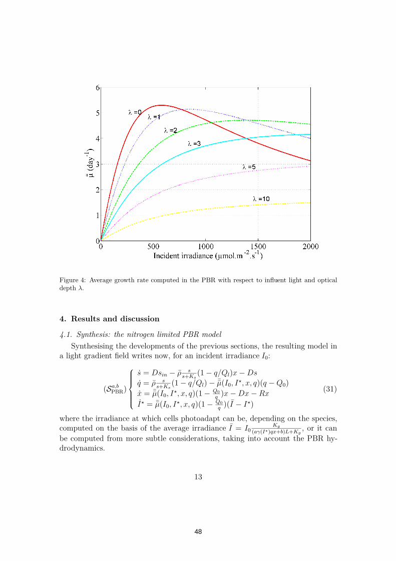
Figure 4: Average growth rate computed in the PBR with respect to influent light and opticaldepth λ.
4. Results and discussion
4.1. Synthesis: the nitrogen limited PBR model
Synthesising the developments of the previous sections, the resulting model ina light gradient field writes now, for an incident irradiance I0:
(Sa,bPBR)
s = Dsin − ρ ss+Ks
(1− q/Ql)x−Dsq = ρ s
s+Ks(1− q/Ql)− ¯µ(I0, I
⋆, x, q)(q −Q0)
x = ¯µ(I0, I⋆, x, q)(1− Q0
q)x−Dx−Rx
I⋆ = ¯µ(I0, I⋆, x, q)(1− Q0
q)(I − I⋆)
(31)
where the irradiance at which cells photoadapt can be, depending on the species,computed on the basis of the average irradiance I = I0
Kg(aγ(I⋆)qx+b)L+Kg
, or it can
be computed from more subtle considerations, taking into account the PBR hy-drodynamics.
13
48
The average growth function is given by equation (27) and (28) for models(SaPBR) and (SbPBR), respectively.
4.2. Model calibration
The way the model is designed makes its calibration rather straightforward.The idea is based on the fact that simpler models are easier to calibrate. Theprocedure thus consists in progressively improving the model accuracy by usingthe simple models calibration to initiate the identification of the more complexmodels, moving then from Droop model to the PBR model SbPBR. The first stepconsists in calibrating the parameters of Droop model on the basis of Property1. The observation of the nitrogen quota during phases of replete and depletedinorganic nitrogen in the culture gives an estimate of the minimal and maximalnitrogen quota of Droop model, and thus, using equations (4) and (6) togetherwith an estimate of the (average) growth rate in conditions of nutrient repletion,we get parameters Q0, ρm and µ. Parameter Ks is determined from additionaluptake experiments. This first raw calibration of the Droop model is used as afirst guess for the more detailed model parameters. Droop’s parameter can nowbe seen as the average value of the detailed model. For example, the averagevalue of ¯µ() in the PBR model is µ in Droop’s model. The first guess of the PBRparameters are then chosen such that, taking into account the measured averagelight intensity and Chl:C ratio, we have:
µ =1
T
∫ T
0
¯µ(I†0, I⋆, x†, q†)dτ (32)
where the values with † are measurements. This approach, leads to a first sketchwhich generates simulation results improving Droop’s predictions. A final refine-ment, where a least square quality criterion is minimised by Levenberg-Marquardtalgorithm (function lsqcurvefit under Matlab R©) produces the final values of theparameters.
Model is calibrated with the experimental data of Flynn et al. (1994) forIsochrysis galbana grown with ammonium in a batch PBR on a 12:12 light/darkcycle under incident illumination of 100 µmol.m−2.s−1. The resulting parametervalues are given in table 1.
4.3. Model validation
Model simulations are shown on figure 5. The good adequation obtained withthe experimental data illustrates the fact that the model calibration is ratherstraightforward. The model demonstrates a great ability to properly reproducesuch data set. The simulations of particulate nitrogen seem to underestimate a bitthe measured values. This results from a leak in the nitrogen balance, from theinitial ammonium concentration to the final particulate nitrogen concentration.
14
49

Parameter Value Unitµ 1.7 day−1
Q0 0.050 gN. gC−1
Ql 0.25 gN.gC−1
K∗sI 1.4 µmol.m−2.s−1
KbiI 295 µmol.m−2.s−1
ρ 0.073 gN.gC−1.day−1
Ks 0.0012 gN.m−3
R 0.0081 day−1
δ 1 –γmax 0.57 gChl.gN−1
kI∗ 63 µmol.m−2.s−1
a 16.2 m2.gChl−1
b 0.087 m−1
Table 1: Parameter values used for the simulation of the PBR model
This experimental imbalance in the nitrogen may also have impacted the accuracyon the chlorophyll a.
These results can be compared with the simulation results obtained by Smithand Yamanaka (2007) that use both biological models of Geider et al. (1998) andof Pahlow (2005), where the light distribution was added as an extra layer in themodel. Our model prediction is of comparable quality, while it explicitly representsthe coupling between microalgae physiology and light transfer properties on thePBR.
4.4. discussion
Light heterogeneity in the medium induces a complex photoacclimation pro-cess resulting from both a negative and a positive feedback. After an incident lightshift, the biomass concentration increases and so do the pigments in the medium.It results in reducing the range of average light increase compared to the incidentlight shift. This negative feedback is completed by a positive feedback, since pho-toacclimation to a higher irradiance leads to a reduction of the pigment contentand thus a higher light penetration. This shows that modelling is the only possi-bility to quantitatively describe the dynamics in a high density PBR. This is allthe more crucial since microalgae are necessarily in a permanent dynamical regimeinduced by the daily light variations. As a consequence, such model is necessary toextrapolate from the cell characteristics to photobioreactor behaviour. It can alsohelp in assessing and optimising the biomass productivity in outdoor conditions,which are the conditions for autotrophic biofuel production.
15
50

0 5 10 15 20 250
0.05
0.1
0.15
0.2
Time (d)
NH
4 (m
ol/m
3 )
0 5 10 15 20 250
10
20
30
40
Time (d)
Par
ticul
ate
Car
bon
(g C
/m3 )
0 5 10 15 20 250
0.1
0.2
0.3
0.4
0.5
Time (d)
Chl
(g
Chl
/ m3 )
0 5 10 15 20 250
0.5
1
1.5
2
Time (d)
Par
ticul
ate
Nitr
ogen
(g
N/ m
3 )
Figure 5: Simulation of the PBR model and comparison with experimental data from Flynnet al. (1994).
Beyond the prediction capacity of our model, under dynamical variations in-duced by the daily light variation, our approach explains a key point: for highdensity cultures, there is no apparent photoinhibition. This does not mean thatalgae do not photoinhibit, but it means that, because of averaging along the re-actor depth, photoinhibition is not revealed by a standard production versus lightintensity study. However photoinhibition must be avoided, since it results in ahidden loss of productivity that can be evaluated from the decreased apparentaveraged maximum growth rate. Figure 4 also reveals that, for a given light inten-sity, there is an optimal optical depth that leads to the optimum average growthrate.
5. Conclusion
The proposed dynamical model integrates the light gradient in the PBR inorder to represent the coupling between microalgal growth and radiative transfer
16
51
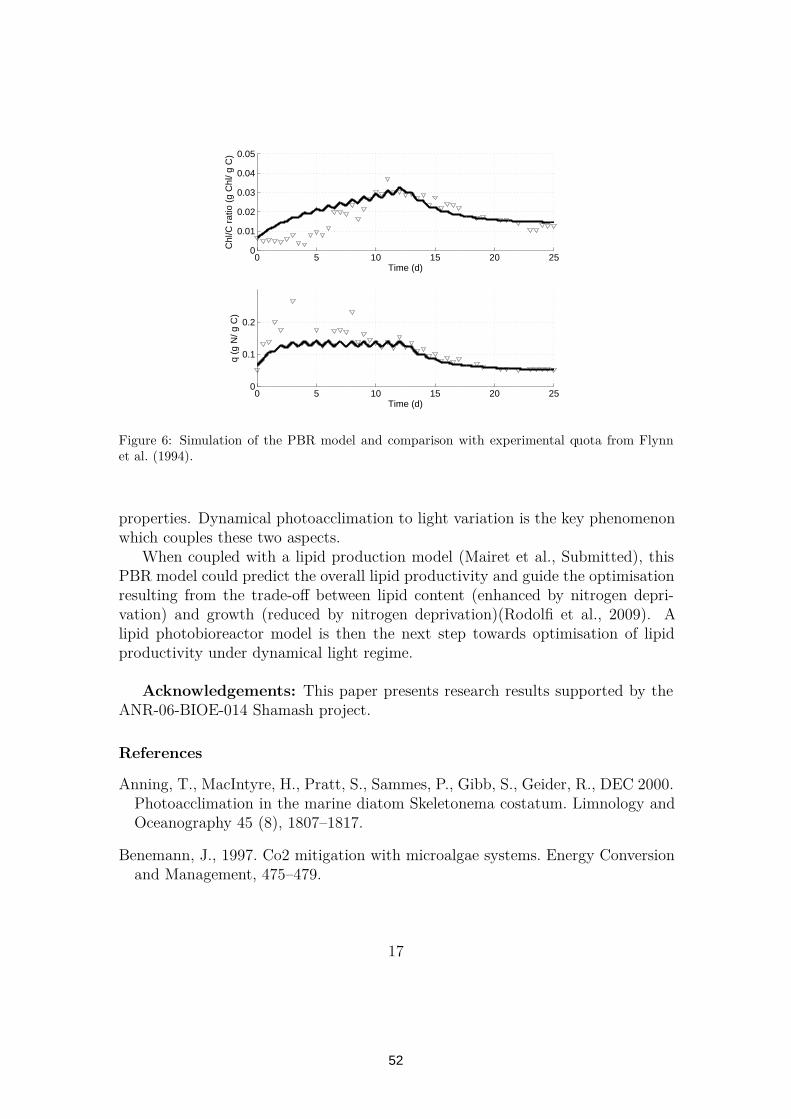
0 5 10 15 20 250
0.01
0.02
0.03
0.04
0.05
Time (d)
Chl
/C r
atio
(g
Chl
/ g C
)
0 5 10 15 20 250
0.1
0.2
Time (d)
q (g
N/ g
C)
Figure 6: Simulation of the PBR model and comparison with experimental quota from Flynnet al. (1994).
properties. Dynamical photoacclimation to light variation is the key phenomenonwhich couples these two aspects.
When coupled with a lipid production model (Mairet et al., Submitted), thisPBR model could predict the overall lipid productivity and guide the optimisationresulting from the trade-off between lipid content (enhanced by nitrogen depri-vation) and growth (reduced by nitrogen deprivation)(Rodolfi et al., 2009). Alipid photobioreactor model is then the next step towards optimisation of lipidproductivity under dynamical light regime.
Acknowledgements: This paper presents research results supported by theANR-06-BIOE-014 Shamash project.
References
Anning, T., MacIntyre, H., Pratt, S., Sammes, P., Gibb, S., Geider, R., DEC 2000.Photoacclimation in the marine diatom Skeletonema costatum. Limnology andOceanography 45 (8), 1807–1817.
Benemann, J., 1997. Co2 mitigation with microalgae systems. Energy Conversionand Management, 475–479.
17
52

Bernard, O., Gouzé, J. L., 1995. Transient Behavior of Biological Loop Models,with Application to the Droop Model. Mathematical Biosciences 127 (1), 19–43.
Bernard, O., Gouzé, J.-L., 1999. Nonlinear qualitative signal processing for biolog-ical systems: application to the algal growth in bioreactors. Math. Biosciences157, 357–372.
Bernard, O., Gouzé, J.-L., 2002. Global qualitative behavior of a class of nonlinearbiological systems: application to the qualitative validation of phytoplanktongrowth models. Artif. Intel. 136, 29–59.
Carvalho, A., Meireles, L., Malcata, F., 2006. Microalgal reactors: A review ofenclosed system designs and performances. Biotechnology Progress 22(6), 1490–1506.
Chisti, Y., 2007. Biodiesel from microalgae. Biotechnology Advances 25, 294–306.
Droop, M. R., 1968. Vitamin B12 and marine ecology. IV. the kinetics of uptakegrowth and inhibition in Monochrysis lutheri. J. Mar. Biol. Assoc. 48 (3), 689–733.
Droop, M. R., 1983. 25 years of algal growth kinetics, a personal view. Botanicamarina 16, 99–112.
Eilers, P., Peeters, J., 1988. A model for the relationship between light intensityand the rate of photosynthesis in phytoplankton. Ecological modelling 42 (3-4),199–215.
Eilers, P., Peeters, J., SEP 1993. Dynamic behavior of a model for photosynthesisand photoinhibition. Ecological modelling 69 (1-2), 113–133.
Flynn, K., Davidson, K., Leftley, J., 1994. Carbon-nitrogen relations at whole-celland free amino-acid levels, during batch growth of isochrysis galbanna (prym-nesiophyceae) under conditions of alternating light and dark. Mar. Biol. 118,229–237.
Franco-Lara, E., Havel, J., F, F., D, D. W.-B., 2006. Model-supported optimizationof phototrophic growth in a stirred-tank photobioreactor. Biotech. Bioeng. 95,1177–1187.
Geider, R., MacIntyre, H., Kana, T., 1996. A dynamic model of photoadaptationin phytoplankton. Limnol Oceanogr 41, 1–15.
18
53

Geider, R., MacIntyre, H., Kana, T., 1998. A dynamic regulatory model of phy-toplanktonic acclimation to light, nutrients, and temperature. Limnol Oceanogr43, 679–694.
Han, B., 2001. Photosynthesis-irradiance response at physiological level: A mech-anistic model. J Theor Biol 213, 121–127.
Huntley, M., Redalje, D., 2007. Co2 mitigation et renewable oil from photosyn-thetic microbes: A new appraisal. Mitigation et Adaptation Strategies for GlobalChange 12, 573 – 608.
Lange, K., Oyarzun, F. J., 1992. The attractiveness of the Droop equations. Math-ematical Biosciences 111, 261–278.
Laws, E., Bannister, T., 1980. Nutrient- and light-limited growth of thalassiosirafluviatilis in continuous culture, with implications for phytoplankton growth inthe ocean. Limnol Oceanogr 25, 457–473.
MacIntyre, H., Kana, T., Anning, T., Geider, R., 2002. Photoacclimation of photo-synthesis irradiance response curves and photosynthetic pigments in microalgaeand cyanobacteria. Journal of Phycology 38 (1), 17–38.
Mairet, F., Bernard, O., Masci, P., Lacour, T., Sciandra, A., Submitted. Mod-elling neutral lipid production by the microalga Isochrysis affinis galbana undernitrogen limitation.
Metting, F., 1996. Biodiversity and application of microalgae. Journal of IndustrialMicrobiology & Biotechnology 17, 477 – 489.
Olaizola, M., 2003. Commercial development of microalgal biotechnology: fromthe test tube to the marketplace. Biomolecular Engineering 20, 459–466.
Pahlow, M., 2005. Linking chlorophyll-nutrient dynamics to the Redfield N : Cratio with a model of optimal phytoplankton growth. marine ecology-progressseries 287, 33–43.
Pawlowski, L., 2004. Modélisation de l’incorporation du carbone photosynthétiqueen environnement marin contrôlé par ordinateur. Ph.D. thesis, Université Pierreet Marie Curie, Paris VI.
Pottier, L., Pruvost, J., Deremetz, J., Cornet, J.-F., Legrand, J., Dussap, C.,2005. A fully predictive model for one-dimensional light attenuation by chlamy-domonas reinhardtii in a torus photobioreactor. Biotechnology and Bioengineer-ing 91, 569–582.
19
54

Pruvost, J., Pottier, L., Legrand, J., 2006. Numerical investigation of hydrody-namic and mixing conditions in a torus photobioreactor. Chemical EngineeringScience 61, 4476–4489.
Pruvost, J., Van Vooren, G., Cogne, G., Legrand, J., 2009. Investigation ofbiomassand lipids production with neochloris oleoabundans in photobioreactor. Biores.Technol. 100, 5988–5995.
Pulz, O., 2001. Photobioreactors: production systems for phototrophic microor-ganisms. Applied Microbiology et Biotechnology 57, 287–293.
Rodolfi, L., Zittelli, G. C., Bassi, N., Padovani, G., Biondi, N., Bonini, G., Tredici,M. R., JAN 1 2009. Microalgae for Oil: Strain Selection, Induction of Lipid Syn-thesis and Outdoor Mass Cultivation in a Low-Cost Photobioreactor. Biotechnol.Bioeng. 102 (1), 100–112.
Sciandra, A., Gostan, J., Collos, Y., Descolas-Gros, C., Leboulanger, C., Martin-Jézéquel, V., Denis, M., Lefèvre, D., C. Copin, C., Avril, B., 1997. Growthcompensating phenomena in continuous cultures of Dunaliella tertiolecta limitedsimultaneously by light and nitrate. Limnol. Oceanogr. 46, 1325–1339.
Sciandra, A., Lazzara, L., Claustre, H., Babin, M., 2000. Responses of the growthrate, pigment composition and optical properties of cryptomonas sp. to lightand nitrogen stresses. Mar. Ecol. Prog. Ser. 201, 107–120.
Sciandra, A., Ramani, P., 1994. The limitations of continuous cultures with lowrates of medium renewal per cell. J. Exp. Mar. Biol. Ecol. 178, 1–15.
Sialve, B., Bernet, N., Bernard, O., 2009. Anaerobic digestion of microalgae asa necessary step to make microalgal biodiesel sustainable. Biotech. Advances27 (4), 409–416.
Smith, S. L., Yamanaka, Y., 2007. Optimization-based model of multinutrientuptake kinetics. Limnology and Oceanography 52 (4), 1545–1558.
Spoehr, H. A., Milner, H. W., 1949. The chemical composition of chlorella: effectof environmental conditions. Plant Physiol. 24, 120 – 149.
Stramski, D., Sciandra, A., Claustre, H., 2002. Effects of temperature, nitrogen,and light limitation on the optical properties of the marine diatom thalassiosirapseudonana. Limnol. Oceanogr. 47, 392–403.
Suh, I., Lee, S., 2003. A light distribution model for an internally radiating pho-tobioreactor. Biotech. Bioeng. 82, 180–189.
20
55

Thompson, P. A., Harrison, P. J., Whyte, J. N. C., 1990. Influence of irradiance onthe fatty acid composition of phytoplankton. Journal of Phycology 26, 278–288.
Turpin, D., 1991. Effects of inorganic n availability on algal photosynthesis andcarbon metabolism. J Phycol 27, 14–20.
Vatcheva, I., deJong, H., Bernard, O., Mars, N., 2006. Experiment selection for thediscrimination of semi-quantitative models of dynamical systems. Artif. Intel.170, 472–506.
21
56
Modelling lipid production in microalgae
Francis Mairet∗
Olivier Bernard∗
Pierre Masci∗
Thomas Lacour∗∗
Antoine Sciandra∗∗
∗ COMORE-INRIA, BP93, 06902 Sophia-Antipolis Cedex, France(e-mail: [email protected]).
∗∗ LOV, UMR 7093, BP28, 06234 Villefranche-sur-mer, France
Abstract: Microalgae offer potentially great opportunities for producing biofuel. In order tooptimize triglyceride production, this article proposes a dynamical model of microalgal lipidproduction. In this model, intracellular carbon is divided between a functional pool and twostorage pools (sugars and neutral lipids). The various intracellular carbon flows between thesepools lead to a complex dynamic with a strong discrepancy between accumulation and reuse ofneutral lipids. This generates an hysteresis which has been observed experimentally. The modelhas been validated with experiments of Isochrysis affinis galbana (T. iso) culture under differentnitrogen limitation conditions.
Keywords: phytoplankton, growth model, nitrogen starvation, neutral lipid, biofuel
1. INTRODUCTION
Various photosynthetic microorganisms (microalgae orcyanobacteria) have shown an ability to synthesize andaccumulate considerable amounts of lipids [Chisti 2007].Indeed, the photosynthetic yield of these microorgan-isms (abusively gathered under the name ”microalgae”) ishigher than for terrestrial plants whose growth is limitedby CO2 availability. Its leads to algal biomass productivi-ties of several tens of dry biomass tons per hectare and peryear [Huntley and Redalje 2007]. When combined with ahigh neutral lipid content [Metting 1996], microalgae canpotentially produce biofuel in a range of magnitude higherthan for terrestrial plants. This potential has led someauthors to consider that microalgae could be one of themain biofuel producers in the future [Huntley and Redalje2007, Chisti 2007].
However, the culture of algae is not straightforward andsuffers from many limitations [Pulz 2001, Carvalho et al.2006]. For example, a nitrogen limitation increases the celllipid content but it also strongly affects the growth rate.The lipid productivity, which is the consequence of thesetwo factors, needs a trade off between biomass productionand oil content.
The main objective of this work is to propose a newmodel for lipid production under nitrogen stress which willguide the research of an optimisation strategy. The modelmust thus find a trade off between realism, in order toaccurately represent the key variables of the process, andsimplicity so that it can be mathematically tractable andsuitable to solve optimal control problems. The simplestmodel for describing growth of a population of microalgaelimited by a nutrient (e.g. nitrogen or phosphorus) is theDroop model [Droop 1968, 1983]. This models assumesthat the growth rate depends on the internal concentrationof the limiting element. More accurate models have beenproposed to deal with the coupling between nitrogen andcarbon assimilation in various light conditions [Geider
et al. 1998, Faugeras et al. 2004, Pahlow 2005]. Howevernone of these models predicted the lipid concentration and,to our knowledge, the model which is presented in thiswork is the first dealing with neutral lipid production bymicroalgae. The main objective of this dynamical modelis to identify conditions that optimise the lipid synthesis.
The article is structured as follows: after a material andmethods section, the model assumptions are detailled andthen the resulting model equations are presented. Then,we describe the calibration procedure and we compare themodel with experimental data of a Isochysis galbana cul-ture, with different nitrogen limitations. Finally, a sectionis devoted to the analysis of the model behavior.
2. MATERIAL AND METHODS
2.1 Culturing device
Cultures of Isochrysis affinis galbana, (clone T-iso) weregrown in 5 l cylindrical vessels at constant temperature(22.5◦C), ligth (430±30 µmol.m−2.s−1 in the centre of theculture vessel) and pH (maintained at 8.0 by automaticinjection of CO2). The experiment consists in imposingnitrogen limitation through a succession of dilution rateschanges followed by transient periods to reach the equilib-rium. Finally, dilution was stopped to obtain a nitrogenstarvation. Figure 1 presents the operating conditions.
2.2 Measurements
The following measurements were performed: nitrate con-centrations (Technicon Auto-analyser), biovolumes (opti-cal particle counter Hiac/Royco), concentrations of partic-ulate carbon and nitrogen (CHN analyser, PerkinElmer),total carbohydrates concentrations (by the phenol method),and neutral lipid (column chromatography on silica gel,Extract-Clean, Alltech). A correlation between biovolumemeasurements and particulate carbon is used to convert
57
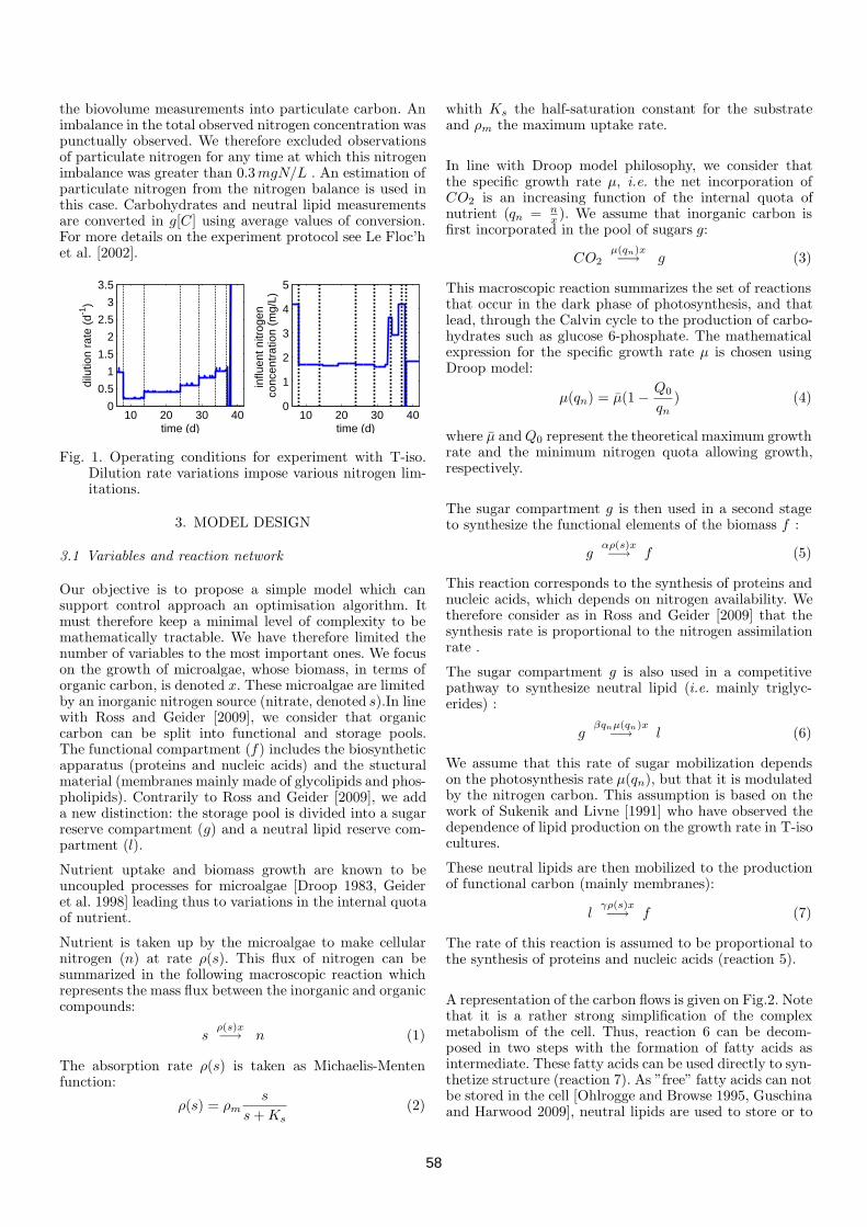
the biovolume measurements into particulate carbon. Animbalance in the total observed nitrogen concentration waspunctually observed. We therefore excluded observationsof particulate nitrogen for any time at which this nitrogenimbalance was greater than 0.3 mgN/L . An estimation ofparticulate nitrogen from the nitrogen balance is used inthis case. Carbohydrates and neutral lipid measurementsare converted in g[C] using average values of conversion.For more details on the experiment protocol see Le Floc’het al. [2002].
10 20 30 400
0.5
1
1.5
2
2.5
3
3.5
time (d)
dilu
tion
rate
(d-1
)
10 20 30 400
1
2
3
4
5
time (d)
influ
ent n
itrog
en
conc
entr
atio
n (m
g/L)
Fig. 1. Operating conditions for experiment with T-iso.Dilution rate variations impose various nitrogen lim-itations.
3. MODEL DESIGN
3.1 Variables and reaction network
Our objective is to propose a simple model which cansupport control approach an optimisation algorithm. Itmust therefore keep a minimal level of complexity to bemathematically tractable. We have therefore limited thenumber of variables to the most important ones. We focuson the growth of microalgae, whose biomass, in terms oforganic carbon, is denoted x. These microalgae are limitedby an inorganic nitrogen source (nitrate, denoted s).In linewith Ross and Geider [2009], we consider that organiccarbon can be split into functional and storage pools.The functional compartment (f) includes the biosyntheticapparatus (proteins and nucleic acids) and the stucturalmaterial (membranes mainly made of glycolipids and phos-pholipids). Contrarily to Ross and Geider [2009], we adda new distinction: the storage pool is divided into a sugarreserve compartment (g) and a neutral lipid reserve com-partment (l).
Nutrient uptake and biomass growth are known to beuncoupled processes for microalgae [Droop 1983, Geideret al. 1998] leading thus to variations in the internal quotaof nutrient.
Nutrient is taken up by the microalgae to make cellularnitrogen (n) at rate ρ(s). This flux of nitrogen can besummarized in the following macroscopic reaction whichrepresents the mass flux between the inorganic and organiccompounds:
sρ(s)x−→ n (1)
The absorption rate ρ(s) is taken as Michaelis-Mentenfunction:
ρ(s) = ρm
s
s + Ks
(2)
whith Ks the half-saturation constant for the substrateand ρm the maximum uptake rate.
In line with Droop model philosophy, we consider thatthe specific growth rate µ, i.e. the net incorporation ofCO2 is an increasing function of the internal quota ofnutrient (qn = n
x). We assume that inorganic carbon is
first incorporated in the pool of sugars g:
CO2µ(qn)x−→ g (3)
This macroscopic reaction summarizes the set of reactionsthat occur in the dark phase of photosynthesis, and thatlead, through the Calvin cycle to the production of carbo-hydrates such as glucose 6-phosphate. The mathematicalexpression for the specific growth rate µ is chosen usingDroop model:
µ(qn) = µ(1 −Q0
qn
) (4)
where µ and Q0 represent the theoretical maximum growthrate and the minimum nitrogen quota allowing growth,respectively.
The sugar compartment g is then used in a second stageto synthesize the functional elements of the biomass f :
gαρ(s)x−→ f (5)
This reaction corresponds to the synthesis of proteins andnucleic acids, which depends on nitrogen availability. Wetherefore consider as in Ross and Geider [2009] that thesynthesis rate is proportional to the nitrogen assimilationrate .
The sugar compartment g is also used in a competitivepathway to synthesize neutral lipid (i.e. mainly triglyc-erides) :
gβqnµ(qn)x
−→ l (6)
We assume that this rate of sugar mobilization dependson the photosynthesis rate µ(qn), but that it is modulatedby the nitrogen carbon. This assumption is based on thework of Sukenik and Livne [1991] who have observed thedependence of lipid production on the growth rate in T-isocultures.
These neutral lipids are then mobilized to the productionof functional carbon (mainly membranes):
lγρ(s)x−→ f (7)
The rate of this reaction is assumed to be proportional tothe synthesis of proteins and nucleic acids (reaction 5).
A representation of the carbon flows is given on Fig.2. Notethat it is a rather strong simplification of the complexmetabolism of the cell. Thus, reaction 6 can be decom-posed in two steps with the formation of fatty acids asintermediate. These fatty acids can be used directly to syn-thetize structure (reaction 7). As ”free” fatty acids can notbe stored in the cell [Ohlrogge and Browse 1995, Guschinaand Harwood 2009], neutral lipids are used to store or to
58
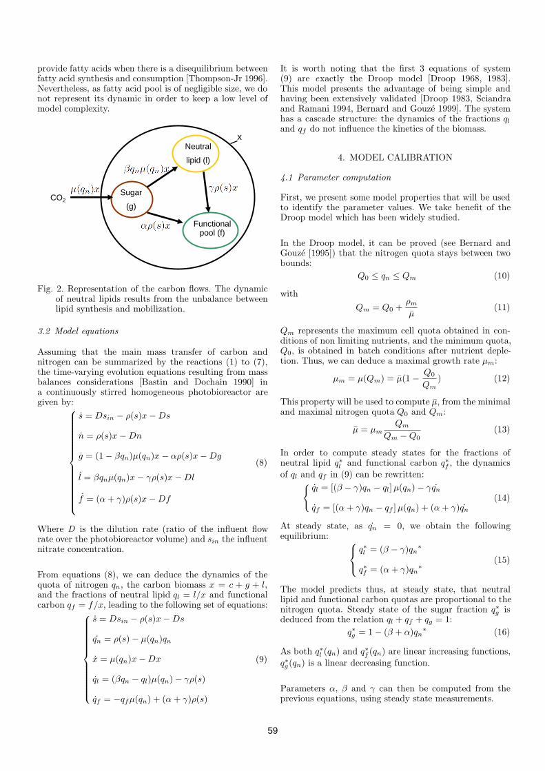
provide fatty acids when there is a disequilibrium betweenfatty acid synthesis and consumption [Thompson-Jr 1996].Nevertheless, as fatty acid pool is of negligible size, we donot represent its dynamic in order to keep a low level ofmodel complexity.
Neutral
lipid (l)
x
Functional pool (f)
CO2Sugar
(g)
Fig. 2. Representation of the carbon flows. The dynamicof neutral lipids results from the unbalance betweenlipid synthesis and mobilization.
3.2 Model equations
Assuming that the main mass transfer of carbon andnitrogen can be summarized by the reactions (1) to (7),the time-varying evolution equations resulting from massbalances considerations [Bastin and Dochain 1990] ina continuously stirred homogeneous photobioreactor aregiven by:
s = Dsin − ρ(s)x − Ds
n = ρ(s)x − Dn
g = (1 − βqn)µ(qn)x − αρ(s)x − Dg
l = βqnµ(qn)x − γρ(s)x − Dl
f = (α + γ)ρ(s)x − Df
(8)
Where D is the dilution rate (ratio of the influent flowrate over the photobioreactor volume) and sin the influentnitrate concentration.
From equations (8), we can deduce the dynamics of thequota of nitrogen qn, the carbon biomass x = c + g + l,and the fractions of neutral lipid ql = l/x and functionalcarbon qf = f/x, leading to the following set of equations:
s = Dsin − ρ(s)x − Ds
qn = ρ(s) − µ(qn)qn
x = µ(qn)x − Dx
ql = (βqn − ql)µ(qn) − γρ(s)
qf = −qfµ(qn) + (α + γ)ρ(s)
(9)
It is worth noting that the first 3 equations of system(9) are exactly the Droop model [Droop 1968, 1983].This model presents the advantage of being simple andhaving been extensively validated [Droop 1983, Sciandraand Ramani 1994, Bernard and Gouze 1999]. The systemhas a cascade structure: the dynamics of the fractions ql
and qf do not influence the kinetics of the biomass.
4. MODEL CALIBRATION
4.1 Parameter computation
First, we present some model properties that will be usedto identify the parameter values. We take benefit of theDroop model which has been widely studied.
In the Droop model, it can be proved (see Bernard andGouze [1995]) that the nitrogen quota stays between twobounds:
Q0 ≤ qn ≤ Qm (10)
with
Qm = Q0 +ρm
µ(11)
Qm represents the maximum cell quota obtained in con-ditions of non limiting nutrients, and the minimum quota,Q0, is obtained in batch conditions after nutrient deple-tion. Thus, we can deduce a maximal growth rate µm:
µm = µ(Qm) = µ(1 −Q0
Qm
) (12)
This property will be used to compute µ, from the minimaland maximal nitrogen quota Q0 and Qm:
µ = µm
Qm
Qm − Q0(13)
In order to compute steady states for the fractions ofneutral lipid q∗l and functional carbon q∗f , the dynamics
of ql and qf in (9) can be rewritten:{
ql = [(β − γ)qn − ql]µ(qn) − γqn
qf = [(α + γ)qn − qf ]µ(qn) + (α + γ)qn
(14)
At steady state, as qn = 0, we obtain the followingequilibrium:
q∗l = (β − γ)qn∗
q∗f = (α + γ)qn∗
(15)
The model predicts thus, at steady state, that neutrallipid and functional carbon quotas are proportional to thenitrogen quota. Steady state of the sugar fraction q∗g isdeduced from the relation ql + qf + qg = 1:
q∗g = 1 − (β + α)qn∗ (16)
As both q∗l (qn) and q∗f (qn) are linear increasing functions,
q∗g(qn) is a linear decreasing function.
Parameters α, β and γ can then be computed from theprevious equations, using steady state measurements.
59

4.2 Parameter estimation
We have decoupled the estimation into two groups ofparameters: the Droop parameters (Q0, µ, ρm, Ks) andthe intracellular carbon flow parameters (α, β, and γ). TheDroop parameters can be easily determined, on the basisof dedicated experimental conditions. Then, the carbonparameters are identified using steady state observations.
The minimal nitrogen quota Q0 is obtained from thenitrogen quota measurement during nitrate starvation (atthe end of the experiment). The maximum nitrogen quotaQm and specific growth rate µm are estimated directlyfrom the nitrogen quota measurements and the dilutionrate during non-limited growth (see Fig. 3). The maximalabsorption rate ρm and growth parameter µ were obtainedwith relations (11) and (13). The half-saturation constantKs = 0.018 mg[N ]/L is taken from previous experiments(data not shown).
The second step of the calibration procedure concerns theintracellular carbon flow parameters. The data obtainedat steady state for the several dilution rates are used todetermine, thanks to equations (15), the parameters α, β,and γ. Using an estimation of the slopes of q∗l (qn) andq∗f (qn) lines, we obtain a system of two equations withthree unknown parameters. We have therefore one freedomdegree to fit the transient behavior of the model to the datausing a minimization algorithm.
The results of the calibration are given in table 1.
Table 1. Parameters obtained by the calibra-tion of the model
Parameter Value
Minimal nitrogen quota Q0 0.05 mg[N ].mg[C]−1
Maximal nitrogen quota Qm 0.11 mg[N ].mg[C]−1
Maximal growth rate µm 1 d−1
Protein synthesis coefficient α 2.9 mg[C].mg[N ]−1
Fatty acid synthesis coefficient β 3.75 −
Fatty acid mobilisation coefficient γ 2.0 mg[C].mg[N ]−1
Half-saturation constant Ks 0.018 mg[N ].L−1
Theoretical maximum growth rate µ† 1.83 d−1
Maximal uptake rate ρm
† 0.11 mg[N ].mg[C]−1.d−1
† : Parameters computed from Q0, Qm and µm
5. SIMULATION AND COMPARISON WITHEXPERIMENTAL DATA
Continuous culture of T-iso is used in order to assessthe ability of the model to reproduce experimental data.Results shown in Fig. 3 demonstrate that the model re-produces quite accurately the dynamics of s, qn and x.This corroborates the fact that the Droop model has beenwidely validated [Droop 1983, Sciandra and Ramani 1994,Bernard and Gouze 1999] for its aptitude to predict bothbiomass and remaining inorganic nitrogen. The simulatedintracellular carbon distribution between sugar, neutrallipid and functional pool also accurately follows the ex-perimental records (Fig. 4).
10 15 20 25 30 35 400
1
2
3
NO
3 (m
g N
/L)
10 15 20 25 30 35 400.04
0.06
0.08
0.1
0.12
nitr
ogen
quo
ta (
g N
/g C
)
10 15 20 25 30 35 4010
20
30
40
50
60
time (d)
Bio
mas
s (m
g C
/L)
Fig. 3. Comparison of the Droop model with the dataof T-iso culture under various nitrogen conditions.Nitrogen quota is directly measured (red diamond) orestimated from nitrogen balance (green circle). Car-bon biomass is measured (red diamond) and deducedfrom biovolume measurements (green circle). Verticallines indicate dilution rate changes.
6. ANALYSIS OF THE MODEL BEHAVIOR
In this section, we analyse the behavior of the modelcompared with the experimental data in order to explainthe complex dynamic of neutral lipid quota.
6.1 Steady state
Equation (15) shows that the neutral lipid is proportionalto the nitrogen quota in stabilized culture. This result isvalidated with the experimental data (see Fig. 5). Thesteady states obtained in chemostat mode through thevarious dilution rates indeed show that the lipid quota atequilibrium is proportional to the nitrogen quota.
6.2 Unbalanced conditions
Let us consider a situation where the cells are in a steadystate given by a high nitrogen content qn
∗1. If the dilution
rate is decreased, the cells should undergo a decrease oftheir nitrogen quota down to a value qn
∗2 < qn
∗1. This
means that, during this transient, we have ˙qn < 0. Usingequation of ql in (14), the dynamic of z = ql − (β − γ)qn
is:
z = −zµ(qn) − βqn (17)
As z is initialy null, z remains nonnegative during thistransient so that ql is above the line of equation ql = (β −
60
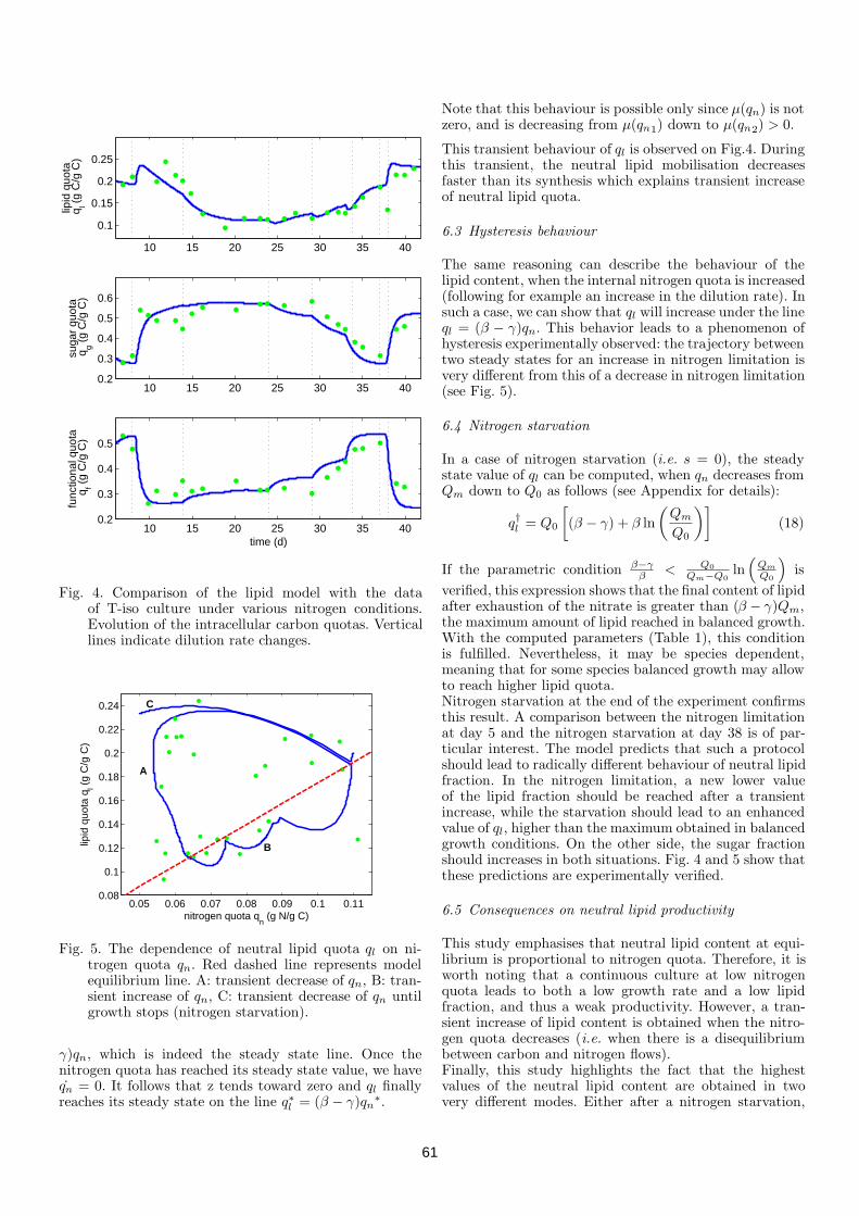
10 15 20 25 30 35 40
0.1
0.15
0.2
0.25
lipid
quo
ta q
l (g
C/g
C)
10 15 20 25 30 35 400.2
0.3
0.4
0.5
0.6
suga
r qu
ota
qg (
g C
/g C
)
10 15 20 25 30 35 400.2
0.3
0.4
0.5
func
tiona
l quo
ta q
f (g
C/g
C)
time (d)
Fig. 4. Comparison of the lipid model with the dataof T-iso culture under various nitrogen conditions.Evolution of the intracellular carbon quotas. Verticallines indicate dilution rate changes.
0.05 0.06 0.07 0.08 0.09 0.1 0.110.08
0.1
0.12
0.14
0.16
0.18
0.2
0.22
0.24
lipid
quo
ta q
l (g
C/g
C)
nitrogen quota qn (g N/g C)
C
A
B
Fig. 5. The dependence of neutral lipid quota ql on ni-trogen quota qn. Red dashed line represents modelequilibrium line. A: transient decrease of qn, B: tran-sient increase of qn, C: transient decrease of qn untilgrowth stops (nitrogen starvation).
γ)qn, which is indeed the steady state line. Once thenitrogen quota has reached its steady state value, we haveqn = 0. It follows that z tends toward zero and ql finallyreaches its steady state on the line q∗l = (β − γ)qn
∗.
Note that this behaviour is possible only since µ(qn) is notzero, and is decreasing from µ(qn1) down to µ(qn2) > 0.
This transient behaviour of ql is observed on Fig.4. Duringthis transient, the neutral lipid mobilisation decreasesfaster than its synthesis which explains transient increaseof neutral lipid quota.
6.3 Hysteresis behaviour
The same reasoning can describe the behaviour of thelipid content, when the internal nitrogen quota is increased(following for example an increase in the dilution rate). Insuch a case, we can show that ql will increase under the lineql = (β − γ)qn. This behavior leads to a phenomenon ofhysteresis experimentally observed: the trajectory betweentwo steady states for an increase in nitrogen limitation isvery different from this of a decrease in nitrogen limitation(see Fig. 5).
6.4 Nitrogen starvation
In a case of nitrogen starvation (i.e. s = 0), the steadystate value of ql can be computed, when qn decreases fromQm down to Q0 as follows (see Appendix for details):
q†l = Q0
[
(β − γ) + β ln
(
Qm
Q0
)]
(18)
If the parametric condition β−γβ
< Q0
Qm−Q0
ln(
Qm
Q0
)
is
verified, this expression shows that the final content of lipidafter exhaustion of the nitrate is greater than (β − γ)Qm,the maximum amount of lipid reached in balanced growth.With the computed parameters (Table 1), this conditionis fulfilled. Nevertheless, it may be species dependent,meaning that for some species balanced growth may allowto reach higher lipid quota.Nitrogen starvation at the end of the experiment confirmsthis result. A comparison between the nitrogen limitationat day 5 and the nitrogen starvation at day 38 is of par-ticular interest. The model predicts that such a protocolshould lead to radically different behaviour of neutral lipidfraction. In the nitrogen limitation, a new lower valueof the lipid fraction should be reached after a transientincrease, while the starvation should lead to an enhancedvalue of ql, higher than the maximum obtained in balancedgrowth conditions. On the other side, the sugar fractionshould increases in both situations. Fig. 4 and 5 show thatthese predictions are experimentally verified.
6.5 Consequences on neutral lipid productivity
This study emphasises that neutral lipid content at equi-librium is proportional to nitrogen quota. Therefore, it isworth noting that a continuous culture at low nitrogenquota leads to both a low growth rate and a low lipidfraction, and thus a weak productivity. However, a tran-sient increase of lipid content is obtained when the nitro-gen quota decreases (i.e. when there is a disequilibriumbetween carbon and nitrogen flows).Finally, this study highlights the fact that the highestvalues of the neutral lipid content are obtained in twovery different modes. Either after a nitrogen starvation,
61

or at maximum growth rate in non limiting conditions.This provides an hint to identify the optimal productivityconditions, which are probably a species dependent combi-nation of these two working modes. The model simplicitywill be the key point to make the optimisation study, froma mathematical point of view, tractable.
7. CONCLUSIONS
We have proposed a new model for neutral lipid productionby microalgae. The strength of this model is to describeaccurately both the steady state and the transient phases.The model catches the different dynamics encountered invarious physiological conditions from low nitrogen limita-tion to starvation. The model, based on a Droop modelprinciple, has a minimal degree of complexity so that itcan be mathematical analysed. This models highlights andexplains the phenomenon of hysteresis in neutral lipidproduction which has been experimentally verified.
The model must be assessed and validated with othermicroalgal species. This model will then be used to predictand optimize neutral lipid production in the perspective oflarge scale biofuel production. It may also endorse a modelbased closed loop control in order to on-line implement theoptimal strategy [Mailleret et al. 2005].
REFERENCES
Bastin, G. and Dochain, D. (1990). On-line estimationand adaptive control of bioreactors. Elsevier, New York.
Bernard, O. and Gouze, J.L. (1995). Transient Behavior ofBiological Loop Models, with Application to the DroopModel. Mathematical Biosciences, 127(1), 19–43.
Bernard, O. and Gouze, J.L. (1999). Nonlinear qualitativesignal processing for biological systems: application tothe algal growth in bioreactors. Math. Biosciences, 157,357–372.
Carvalho, A., Meireles, L., and Malcata, F. (2006). Mi-croalgal reactors: A review of enclosed system designsand performances. Biotechnol Prog, 22(6), 1490–1506.
Chisti, Y. (2007). Biodiesel from microalgae. Biotechnol-ogy Advances, 25, 294–306.
Droop, M.R. (1968). Vitamin B12 and marine ecology.IV. the kinetics of uptake growth and inhibition inMonochrysis lutheri. J. Mar. Biol. Assoc., 48(3), 689–733.
Droop, M.R. (1983). 25 years of algal growth kinetics, apersonal view. Botanica marina, 16, 99–112.
Faugeras, B., Bernard, O., Sciandra, A., and Levy, M.(2004). A mechanistic modelling and data assimila-tion approach to estimate the carbon/chlorophyll andcarbon/nitrogen ratios in a coupled hydrodynamical-biological model. Nonlinear Processes in Geophysics ,11, 515–533.
Geider, R., MacIntyre, H., and Kana, T. (1998). ”adynamic regulatory model of phytoplanktonic acclima-tion to light, nutrients, and temperature. ”. LimnolOceanogr, 43, 679–694.
Guschina, I. and Harwood, J. (2009). Algal Lipids and Ef-fect of the Environment on their Biochemistry. SpringerNew York.
Huntley, M. and Redalje, D. (2007). Co2 mitigationet renewable oil from photosynthetic microbes: A new
appraisal. Mitigation et Adaptation Strategies for GlobalChange, 12, 573 – 608.
Le Floc’h, E., Malara, G., and Sciandra, A. (2002). An au-tomatic device for in vivo absorption spectra acquisitionin phytoplanktonic cultures: application to the studyof photoadaptation to light and nutrient variations. J.Applied Phycol., 14, 435–444.
Mailleret, L., Gouze, J.L., and Bernard, O. (2005). Non-linear control for algae growth models in the chemostat.Bioprocess and Biosystem Engineering, 27, 319–328.
Metting, F. (1996). Biodiversity and application of mi-croalgae. Journal of Industrial Microbiology & Biotech-nology, 17, 477 – 489.
Ohlrogge, J. and Browse, J. (1995). Lipid biosynthesis.The Plant Cell, 7, 957–9708.
Pahlow, M. (2005). Linking chlorophyllnutrient dynamicsto the redfield n:c ratio with a model of optimal phyto-plankton growth. Mar Ecol Prog Ser, 287, 33–43.
Pulz, O. (2001). Photobioreactors: production systems forphototrophic microorganisms. Applied Microbiology etBiotechnology, 57, 287–293.
Ross, O. and Geider, R. (2009). New cell-based modelof photosynthesis and photo-acclimation: accumulationand mobilisation of energy reserves in phytoplankton.Marine Ecology Progress Series, 383, 53–71.
Sciandra, A. and Ramani, P. (1994). The limitations ofcontinuous cultures with low rates of medium renewalper cell. J. Exp. Mar. Biol. Ecol., 178, 1–15.
Sukenik, A. and Livne, A. (1991). Variations in lipid andfatty acid content in relation to acetyl coa carboxylasein the marine prymnesiophyte isochrysis galbana. PlantCell Physiol., 32, 371–378.
Thompson-Jr, G.A. (1996). Lipids and membrane functionin green algae. Biochimica et Biophysica Acta, 1302, 17–45.
Appendix A. COMPUTATION OF FINAL LIPIDQUOTA AFTER NITROGEN STARVATION
The dynamics of qn and ql, once external nitrate have beenexhausted are:
{
qn = −µ(qn)qn
ql = (βqn − ql)µ(qn)(A.1)
Using these equations, the dynamic of v = ql
qn
is:
v =qnql − qlqn
qn2
= −β
qn
qn (A.2)
Integrating from t1 to t2, we obtain:
v2 − v1 =
t2∫
t1
vdt =
qn2∫
qn1
−β
qn
dq = [−β ln qn]qn2
qn1
(A.3)
Now consider a complete starvation from a non limitedequilibrium,i.e. qn1 = Qm, ql1 = (β − γ)Qm, qn2 = Q0
and ql2 = q†l , the last expression becomes:
q†lQ0
−(β − γ)Qm
Qm
= [−β ln qn]Q0
Qm= β ln
Qm
Q0(A.4)
From this equation, we can deduce the expression of q†l .
62

63

64

Chapter 3
Model based productivity
optimization
Productivity of a compound (biomass, oil, methane, ...) is the amount of thiscompound produced in the bioreactor per time unit (and possibly by reactorvolume or surface). In this chapter, we focused on microalgae production, rep-resented by the DPM model.
When we speak about productivity, it is important to say if we are speakingabout volumetric productivity (grams per liter per day) or surface productivity(grams per square meters per day). When dealing with microalgae, we will beinterested by surface productivity, as the sun delivers a given light energy persurface unit. What we want is to maximize the light energy converted intobiomass per day.
When considering surface productivity, we consider a planar geometry withperpendicular light source. The depth of the culture will be W. We are interestedin the quantity of microalgae per surface unit X, which is going to both use andattenuate light, and which can be computed with
X = xW
Based on the Droop Photobioreactor Model (presented in the last chapter), itis possible to compute analytically surface productivities in continuous (chemo-stat) culture.
In the papers presented here we answer rigorously the question "which con-trols (D(t) and sin(t) values) induce maximal productivity?". For reaching thisgoal, our commands are the dilution rate D (input/output flow of water) andinput substrate concentration sin.
The first paper presents a study in a photobioreactor under constant light,at equilibrium. We consider the problem of surface productivity on a givenproduction surface. The model is simplified by assuming that chlorophyll’sphotoadaptation dynamics reached its equilibrium.
The second paper proposes an optimization under day-night cycles. It usesPontryagin’s maximum principle. The complex mathematics involved led usto begin with volumetric productivity optimization, and with a simpler modelassuming that microalgae are not substrate limited.
65

Microalgal biomass surface productivity
optimization based on a photobioreactor
model
Pierre Masci ∗ Frederic Grognard ∗ Olivier Bernard ∗
∗ INRIA- Project COMORE, 2004 route des lucioles, BP 93, 06902Sophia Antipolis Cedex, FRANCE
Tel: +33.4.92.38.78.72 (e-mail: [email protected],[email protected], [email protected]).
Abstract: In this paper we predict and optimize the biomass surface productivity of microalgaein continuous culture under a constant light source. Surface biomass is identified as a keyvariable for assessing productivity: we provide both a mathematical and intuitive explanation.For reaching maximal productivities, biomass surface concentration must be such that growthat the culture bottom (assuming a planar geometry orthogonal to the light source) must beequal to respiration. Therefore the optimal biomass concentration depends both on the incidentlight and culture’s depth. We then show how the chlorophyll/carbon ratio must also be carefullycontrolled to optimize light use in the photobioreactor. Finally, numerical results illustrate ourtheoretical approach.
Keywords: chemostat; microalgae; photobioreactor; model; light attenuation; productivity;biomass; optimization; continuous culture; bioenergy
1. INTRODUCTION
Microalgae cultures have recently received high attentionin the frameworks of food supplements, pharmaceutic pro-duction (Spolaore et al., 2006), as well as CO2 fixationand biofuel production (Huntley and Redalje, 2007; Chisti,2007). Their high actual photosynthetic yield compared toterrestrial plants (whose growth is limited by CO2 avail-ability) leads to large potential algal biomass productionsof several tens of tons per hectare and per year.
The objective of this paper is to give new insights inthe optimization of microalgal biomass production. Thekey aspect when dealing with photobioreactor is the opti-mization of light use. The pigment concentration (mainlychlorophyll) affects the light distribution and use withinthe reactor, so that for too high biomass, light in thephotobioreactor is strongly attenuated and growth is low.Moreover, in case of nitrogen depreciation (necessary toproduce biofuel (Chisti, 2007)) the pigments are affectedand decrease, which modifies light distribution.
In order to find a solution to this non intuitive optimiza-tion problem, analysis based on a modelling approachis required. In this paper, we base our approach on asimplified macroscopic photobioreactor model, dealing notonly with light diffusion, but also with nitrogen use andnitrogen/carbon ratio variation. In order to perform thismathematical analysis we must use models that are simpleso that they are mathematically tractable; we use a sim-plified version of the model proposed in (Bernard et al.,2009, Sub.). Our results are obtained at steady state, andwe prove that these equilibria are achievable. From thismodel, it is shown mathematically that biomass surface
concentration is the key parameter for surface produc-tivity. Then global optimization is computed, and finallynumerical results are presented.
The paper is structured as follows: first, we present themodel dealing with both nitrogen limitation and lightattenuation; then biomass concentration optimization ispresented, followed by chlorophyll/carbon ratio optimiza-tion. A numerical result illustrates the approach. Finally,some ideas are given on how to choose the dilution rate ina continuous culture in order to maximize productivity.
2. A NEW DROOP PHOTOBIOREACTOR MODEL
2.1 Droop model presentation
We here focus on the growth of microalgae limited byinorganic nitrogen availability (provided by nitrate or am-monium), since such conditions are favourable for lipidproduction (Chisti, 2007) or other compounds such as as-taxanthin (Aflalo et al., 2007). The Droop model (Droop,1968, 1983) has been broadly used to take into accountthe ability of microalgae to uncouple substrate absorptionand biomass (x) growth (Droop, 1968, 1983). The growthrate is assumed to depend on the internal quota (q) which,here, is the amount of intracellular nitrogen per biomassunit. This variable yield model writes thus:
s = Dsin − ρ(s)x−Ds
q = ρ(s)− µ(q)q
x = µ(q)x−Dx
(1)
In this model the growth rate functions µ and absorptionfunctions ρ are generally taken as Michaelis-Menten and
66

Droop functions:
ρ(s) = ρms
s+Ks
µ(q) = µ(1−Q0
q)
(2)
where ρm is the maximum uptake rate, Ks is the half satu-ration constant for substrate uptake, µ is the hypotheticalmaximum growth rate (at infinite internal nitrogen quota)and Q0 the minimal cell quota (below this level, no algalgrowth can take place).
It can be proved (Bernard and Gouze, 1995) that theinternal quota will stay between two bounds:
Q0 ≤ q ≤ Qm (3)
Where Qm = Q0+ρm
µ represents the maximum cell quota
obtained in conditions of non limiting nutrients.
The Droop model has been widely studied Bernard andGouze (1995, 2002) and validated (Sciandra and Ramani,1994; Vatcheva et al., 2006). However, it cannot directlybe used in the case of high density photobioreactors fortwo main reasons:
• In its rough form it does not include the effect of lightintensity
• It does not account for the decrease of light due tothe cell density
2.2 Adding light effect on growth
We first consider the case where light is homogeneous inthe reactor, with an intensity I. In the next section we willconsider the case with light attenuation in the reactor.
Light intensity has a direct effect on growth (photosynthe-sis), while nitrogen uptake can continue in the dark. Lightcan then be introduced into parameter µ = µ(I) (Bernardet al., 2009, Sub.):
µ(q, I) = µ(I)(1−Q0
q) = µ
I
I +KI(1−
Q0
q) (4)
where KI is the light half saturation coefficient.
In order to prevent unrealistic quota increase in thedark, we use the down regulation mechanism proposed byLehman et al. (1975):
ρ(s, q) = ρms
s+Ks
Ql − q
Ql −Q0(5)
with Ql > Q0: the uptake rate stops for replete cellsq = Ql.
We also add a constant respiration term r that appliesto both nitrogen and carbon, so that the nitrogen/carbonratio q is not affected:
x = (µ(q, I)− r −D)x
One can verify that the q equation does not change byadding this respiration term.
Finally, the model including light effect reads:
s = Dsin − ρms
s+Ks
Ql−qQl−Q0
x−Ds
q = ρms
s+Ks
Ql−qQl−Q0
− µ II+KI
(q −Q0)
x = µ II+KI
(1− Q0
q )x− rx−Dx
(6)
In the next section, we will take into account the exponen-tial light distribution within the reactor.
2.3 Light attenuation in the photobioreactor
Light is strongly attenuated by the biomass and its pig-ments in the photobioreactor. In this section we representlight distribution and its consequence on the growth rate.The biological and chemical concentrations are still as-sumed to be homogeneous within the photobioreactor.
We consider a planar geometry with perpendicular lightsource. For the sake of explanation simplicity we willconsider a horizontal reactor and speak about ”upperpart” of the reactor on the side of incident light, and”reactor bottom” for the other side. However, our workis also valid for a vertical or diagonal geometry withperpendicular light source. The depth of the culture willbe W .
At equilibrium, it has been shown (Bernard et al., 2009)that the chlorophyll concentration (Chl) is proportionalto the nitrogen content:
Chl = γ(I⋆)qx
γ(I⋆) is a chlorophyll to nitrogen ratio, depending on thelight I⋆ at which the microalgae have been photoadapted.The photoadaptation mechanism is presented in Bernardet al. (Sub.), but it induces a significant complexity andwill be neglected in this study. We thus consider that γ isa constant value which does not depend on light.
To model light attenuation we use a Beer-Lambert law,where the attenuation depends on the chlorophyll content:
I(q, xz) = I0e−aiγqxz (7)
where I0 is the incident light, ai is a light attenuationcoefficient, and z is the depth, so that γqxz represents thechlorophyll per surface unit present above depth z.
From (7) we can compute the average irradiance receivedby the cell culture:
I =I0W
∫ W
0
e−aiγqxzdz
=I0
aiγqxW
(
1− e−qiγqxW)
(8)
which decreases with γqx: this confirms the intuition thathigher biomass or chlorophyll content leads to lower meanlight in the reactor, due to stronger light attenuation.
In the reactor, growth rates vary with depth: in the upperpart of the reactor, higher light causes higher growth thanin the bottom part. The growth rate for a given depth zcan be written:
µz(q, I(q, xz)) = µI(q, xz)
I(q, xz) +KI(1−
Q0
q) (9)
Then, we compute the mean growth rate in the reactor:
µ(q, I0, x) =1
W
∫ W
0
µz(q, I(q, xz))dz
by the change of variable χ = xz it can be rewritten
µ(q, I0, x) =1
xW
∫ xW
0
µz(q, I(q, χ))dχ (10)
so that the mean growth rate depends on the surfacebiomass xW . It represents the total biomass present per
67

surface unit, and will be denoted X = xW . Finally, from(10), we compute the growth rate (now denoted µ(q, I0, X)after a slight abuse of notation):
µ(q, I0, X) = µ(1−Q0/q)aiγqX
ln(
I0+KI
I0e−aiγqX+KI
)
(11)
which depends both on the surface biomass X and thenitrogen/carbon quota q, which is proportional to thechlorophyll/carbon quota at equilibrium. By constructionµ is decreasing withX: the more surface biomass, the morelight attenuation, so that mean growth rate in the reactoris lower. It is interesting to note that µ is increasing withq for low q values, and that it is decreasing with q for highq values: high chlorophyll concentrations lead to high lightattenuation, so that mean growth in the reactor decreases.
It is also interesting to note that for a given q value, thereis a maximal attainable biomass in the reactor, for whichµ(q, I0, X) = r: if such a biomass is attained it cannotincrease anymore due to respiration.
The simplified Droop Photobioreactor Model (DPM) is
s = Dsin − ρms
s+Ks
Ql−qQl−Q0
x−Ds
q = ρms
s+Ks
Ql−qQl−Q0
− µ(q, I0, X)q
x = (µ(q, I0, X)− r −D)x
(12)
This model is a simplified version of the model presentedby Bernard et al. (2009) when photoadaptation is ne-glected. It will be used in the rest of the paper.
3. OPTIMAL CONDITIONS FOR MAXIMIZINGPRODUCTIVITY
3.1 Choosing surface biomass
With model (12), our aim is to compute and optimizebiomass surface productivity (units: mg[C]/m2/day):
P (q, I0, X) = (µ(q, I0, X)− r)X (13)
At equilibrium it is the product between dilution rate(D = µ(I0, q,X)− r) and surface biomass.
Important Remark: productivity is a function of the ni-trogen/carbon quota q and surface biomass X = xW :according to this model a thin culture (W small) with highbiomass concentration x is equivalent to a deep culture (Whigh) with low biomass concentration x, if they have thesame surface biomass.
The reactor can be seen as a solar panel with an energyyield, and losses. The panel’s parameter is X:
• A lowX (low biomass and thin culture) indicates thatmost light is not absorbed by the culture: the panelhas a low energy yield.
• A high X (high biomass and deep culture) indicatesthat in the culture’s bottom there is very little light:most light is absorbed, but in the reactor’s bottomthere are only respiration losses.
Thus, we must choose the best X value to maximize thepanel’s efficiency P .
Theorem 1. For given I0 and q, the optimal X surfacebiomass for maximizing productivity (13) is such thatgrowth rate at depth W is equal to the respiration rate:
µW (q, I(q,Xopt)) = r (14)
This optimal surface biomass concentration can thus becomputed:
Xopt(q) =1
aiγqln
(
I0KI
(µ(q)
r− 1)
)
(15)
Proof: For a given biomass surface concentration X, pro-ductivity can be written from (13) and (10)
P (q, I0, X) =
∫ X
0
(µz(q, I(q, χ))− r)dχ
=
∫ Xopt
0
(µz − r)dχ+
∫ X
Xopt
(µz − r)dχ
= P (q, I0, Xopt) +
∫ X
Xopt
(µz − r)dχ
where the first term is the productivity P (q, I0, Xopt) withXopt chosen according to (14), and the second term isalways negative because µz decreases with X:
• If X is lower than Xopt, then this term would ”re-move” microalgae that grow more than they respire:µz(q, I(q, χ)) > r, ∀χ < Xopt.
• If X is higher than Xopt, then this term would”add” microalgae that respired more than they grow:µz(q, I(q, χ)) < r, ∀χ > Xopt.
so that Xopt maximizes surface productivity.
It is then possible to compute this optimal surface biomassfrom (14), (9) and (7)
µ(q)I0e
−aiγqXopt
I0e−aiγqXopt +KI= r
(with notation µ(q) = µ(1−Q0/q)) we obtain
I0e−aiγqXopt = KI
r
µ(q)− r(16)
which gives the light intensity at depth W , and then leadsto (15).
Since Xopt(q) needs to be positive, it only exists for q >I0µ
I0µ−r(I0+KI)Q0, that is the minimal quota that ensures
that growth can compensate respiration at the reactor’ssurface. 2
3.2 Optimization with both surface biomass and nitrogenquota
We are then left with the choice of an optimal nitro-gen/carbon value q, which can be controlled by adjustingD and sin (see section 4).
• A low quota leads to low potential growth rate µ(q)• A high quota leads to high µ(q) potential growth rate,but also to higher light attenuation, so that the meangrowth rate µ(I0, q,X) in the reactor can be lower.
Thus, an optimal intermediate value must be found.
Theorem 2. There exists only one value qopt maximizingP , provided that the following condition is satisfied:
I0 > KI
[
µ
µ− 2re
r2
µ−2r − 1
]
(17)
Important Remark: (17) is, in practice, always true sinceI0 ≫ KI and µ ≫ r.
68
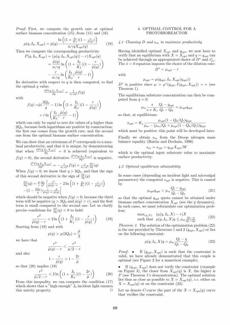
Proof: First, we compute the growth rate at optimalsurface biomass concentration (15), from (11) and (16)
µ(q, I0, Xopt) = µ(q)ln(
(1 + I0KI
)(1− rµ(q) )
)
aiγqXopt(q)(18)
Then we compute the corresponding productivity
P (q, I0, Xopt) = (µ(q, I0, Xopt(q))− r)Xopt(q)
=µ(q)
aiγqln
(
(1 +I0KI
)(1−r
µ(q))
)
−r
aiγqln
(
I0KI
(µ(q)
r− 1)
)
Its derivative with respect to q is then computed, to findthe optimal q value:
∂P (q,I0,Xopt)∂q = 1
aiγq2f(q)
with
f(q) =µ(2Q0
q− 1) ln
(
(1 +I0KI
)(1−r
µ(q))
)
+ r ln
(
I0KI
(µ(q)
r− 1)
)
which can only be equal to zero for values of q higher than2Q0, because both logarithms are positive by construction:the first one comes from the growth rate, and the secondone from the optimal biomass surface concentration.
We can show that an extremum of P corresponds to a max-imal productivity, and that it is unique, by demonstrating
that when∂P (q,I0,Xopt)
∂q = 0 is achieved (equivalent to
f(q) = 0), the second derivative∂2P (q,I0,Xopt)
∂q2 is negative.
∂2P (q,I0,Xopt)∂q2 = − r
aiγq3f(q) + r
aiγq2∂f∂q (q)
When f(q) = 0, we know that q > 2Q0, and that the sign
of this second derivative is the sign of ∂f∂q (q)
∂f∂q (q) =
µrQ0
q2
[
r2
µ(q)−r − 2 ln(
(1 + I0KI
)(1− rµ(q) )
)
−(1− 2Q0
q ) rµ(q)−r
µµ(q)
]
which should be negative when f(q) = 0, because the thirdterm will be negative (q > 2Q0 and µ(q) > r), and the firstterm is small compared to the second one. Let us clarifyprecise conditions for ∂f
∂q (q) < 0 to hold:
r2
µ(q)− r< 2 ln
(
(1 +I0KI
)(1−r
µ(q))
)
(19)
Starting from (19) and with
µ(q) > µ(2Q0) =µ
2we have that
r2
µ(q)− r<
r2
µ/2− rand also
1−r
µ(q)> 1−
2r
µso that (20) implies (19)
r2
µ/2− r< 2 ln
(
(1 +I0KI
)(1−2r
µ)
)
(20)
From this inequality, we can compute the condition (17)which shows that a ”high enough” I0 incident light ensuresthis unicity property. 2
4. OPTIMAL CONTROL FOR APHOTOBIOREACTOR
4.1 Choosing D and sin to maximize productivity
Having identified optimal Xopt and qopt, we now have toverify that an equilibrium with X = Xopt and q = qopt canbe achieved through an appropriated choice of D⋆ and s⋆in.The x = 0 equation imposes the choice of the dilution rate:
D⋆ = µopt − r
withµopt = µ(qopt, I0, Xopt(qopt))
D⋆ is positive since µ > µz(qopt, I(qopt, Xopt)) = r (seeTheorem 1).
The equilibrium substrate concentration can then be com-puted from q = 0:
ρms
s+Ks
Ql − qoptQl −Q0
= µoptqopt
so that, at equilibrium:
sopt = Ksµopt(1−Q0/Ql)qopt
ρm − (ρm/Ql + µopt(1−Q0/Ql))qopt
which must be positive: this point will be developed later.
Finally we obtain sin from the Droop nitrogen massbalance equality (Bastin and Dochain, 1990)
sin = sopt + qoptXopt/W
which is the optimal input substrate value to maximizesurface productivity.
4.2 Optimal equilibrium attainability
In some cases (depending on incident light and microalgalparameters) the computed sopt is negative. This is causedby
µoptqopt > ρmQl − qoptQl −Q0
(21)
so that the optimal qopt quota cannot be attained underbiomass surface concentration Xopt (see the q dynamics).In such cases, we must reformulate our optimization prob-lem:
max(q,X) (µ(q, I0, X)− r)X
such that µ(q, I0, X)q ≤ ρmQl−qQl−Q0
(22)
Theorem 3. The solution of the optimization problem (22)is the one provided by Theorems 1 and 2 (qopt, Xopt) or lieson the following constraint:
µ(q, I0, X)q = ρmQl − q
Ql −Q0(23)
Proof: • If (qopt, Xopt) is such that the constraint isvalid, we have already demonstrated that this couple isoptimal (see Figure 2 for a numerical example).
• If (qopt, Xopt) does not verify the constraint (exampleon Figure 3), the closer from Xopt(q) is X, the higher isP (see Theorem 1’s demonstration). The optimal solutionlies thus as close as possible to X = Xopt(q), i.e. either onX = Xopt(q) or on the constraint (23).
Let us denote C-curve the part of the X = Xopt(q) curvethat verifies the constraint.
69

Because µ(q, I0, X)q is increasing with q and ρmQl−qQl−Q0
is
decreasing with q, we know that any q value on the C-curve verifying the constraint is lower than qopt (whichis too high to verify the constraint). We also know fromTheorem 2 that on the C-curve, the derivative of P withrespect to q is positive for any q < qopt. Because of that,on the C-curve, the maximal P is attained for the highestpossible q: it is the q value lying both on the C-curveand constraint (23). This demonstrates that the optimalproductivity will lie on the constraint.
In this last case sin should be chosen infinite to have sinfinite and ρ(s) = ρm, so that we can be on the constraint.The identification of the optimal (X, q) couple is then notstraightforward, and this case will be the topic of furtheranalysis. 2
Fig. 1. Mean net growth rate (µ − r) in the reactorcomputed from (11), with q = 0, 1g[N ]/g[C] andI0 = 100µ mol quanta. m−2s−1. It is affected by lightattenuation, caused by high biomass concentration.
5. NUMERICAL RESULTS
In the previous sections we have determined that there isa unique optimal (Xopt(qopt), qopt) couple that maximizesthe surface productivity P . In this section we illustratethis result with parameters for the microalgae Isochrysisgalbana.
5.1 Microalgae parameters
The parameter values are taken from Bernard et al. (Sub.)to show productivity results predicted by the model for I.galbana. However, parameters KI and γ (which may varythrough photoacclimation) are computed from averagevalues of the photoadaptation model in Bernard et al.(Sub.).
For all the simulations we use culture’s depth W = 0, 1m.
The growth rate predicted for such a strain is com-puted and plotted in Figure 1, for q = 0.1g[N ]/g[C] andI0 = 100µ mol quanta. m−2s−1. We see on this figurethat because of respiration, there is a maximal biomassx = 4.93g[C]/L for which respiration is equal to growth(µ(X)− r = 0).
Table 1. Parameter values of the lipid modelfor I.galbana culture.
Parameter Value Unit
Q0 0.05 g[N ].g[C]−1
Ql 0.25 g[N ].g[C]−1
µ 1.7 d−1
ρm 0.073 g[N ].g[C]−1.d−1
Ks 0.0012 g[N ]/m3
r 0.07 day−1
KI 20 µ mol quanta. m−2s−1
ai 16.2 m2/g[Chl]γ 0.25 g[Chl]/g[N]
Condition (17) for the unicity of a maximum productivityis verified for I0 > 3, 5µ mol quanta. m−2s−1 which issmall compared to incident light intensities ranging usuallybetween 100µ mol quanta. m−2s−1 to 3000µ mol quanta.m−2s−1.
5.2 Productivity prediction
Productivity was computed with these parameters andwith I0 = 100µ mol quanta. m−2s−1 (Figure 2) and 2000µmol quanta. m−2s−1 (Figure 3).
Fig. 2. Surface biomass productivity for I0 = 100µ molquanta. m−2s−1. The X = Xopt(q) curve is repre-sented by a solid line, and the optimal (qopt, Xopt)couple is represented by a circle. Dotted line indicatesconstraint (23).
On Figure 2 we see that there is an optimal (qopt, Xopt)couple which maximizes productivity. Note that, contrar-ily to the usually assumed hypothesis that higher nitro-gen/carbon ratio leads to higher productivities, we seehere that the optimal conditions do not correspond tonitrogen replete microalgae: for X = Xopt, q > qopt lead tosuboptimal productivities. Thus, depending on the speciesand culture conditions, this result suggests that it could beadvantageous to have slightly nitrogen limited microalgae,so that light attenuation by chlorophyll is weaker and lightis used more efficiently in the photobioreactor.
In Figure 3 we see that the optimal (qopt, Xopt) couple(circle) depends on the incident irradiance (it is not thesame as in the previous figure), and that higher lightintensities lead to higher productivities.
70
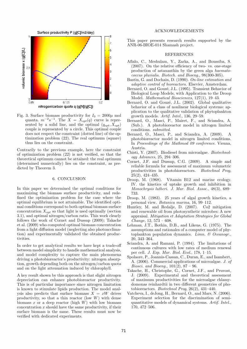
Fig. 3. Surface biomass productivity for I0 = 2000µ molquanta. m−2s−1. The X = Xopt(q) curve is repre-sented by a solid line, and the optimal (qopt, Xopt)couple is represented by a circle. This optimal coupledoes not respect the constraint (dotted line) of the op-timization problem (22). The real optimum (square)thus lies on the constraint.
Contrarily to the previous example, here the constraintof optimization problem (22) is not verified, so that thetheoretical optimum cannot be attained: the real optimum(determined numerically) lies on the constraint, as pre-dicted by Theorem 3.
6. CONCLUSION
In this paper we determined the optimal conditions formaximizing the biomass surface productivity, and rede-fined the optimization problem for the case where theoptimal equilibrium is not attainable. The identified opti-mal conditions correspond to both optimal biomass surfaceconcentration Xopt so that light is used optimally (section3.1), and optimal nitrogen/carbon ratio. This work clearlyfollows the work of Cornet and Dussap (2009); Takacheet al. (2009) who computed optimal biomass concentrationfrom a light diffusion model (neglecting also photoacclima-tion) and experimentally validated the obtained produc-tivities.
In order to get analytical results we have kept a trade-offbetween model simplicity to handle mathematical analysis,and model complexity to capture the main phenomenadriving a photobioreactor’s productivity: nitrogen absorp-tion, growth depending both on the nitrogen/carbon quotaand on the light attenuation induced by chlorophyll.
A key result shown by this approach is that slight nitrogendepreciation can enhance photobioreactor productivity.This is of particular importance since nitrogen limitationis known to stimulate lipids production. The model anal-ysis also predicts that surface biomass X = xW drivesproductivity, so that a thin reactor (low W ) with densebiomass x or a deep reactor (high W ) with low biomassconcentration x should have the same productivity, if theirsurface biomass is the same. These results must now beverified with dedicated experiments.
ACKNOWLEDGEMENTS
This paper presents research results supported by theANR-06-BIOE-014 Shamash project.
REFERENCES
Aflalo, C., Meshulam, Y., Zarka, A., and Boussiba, S.(2007). On the relative efficiency of two- vs. one-stageproduction of astaxanthin by the green alga haemato-coccus pluvialis. Biotech. and Bioeng., 98(300-305).
Bastin, G. and Dochain, D. (1990). On-line estimation andadaptive control of bioreactors. Elsevier, Amsterdam.
Bernard, O. and Gouze, J.L. (1995). Transient Behavior ofBiological Loop Models, with Application to the DroopModel. Mathematical Biosciences, 127(1), 19–43.
Bernard, O. and Gouze, J.L. (2002). Global qualitativebehavior of a class of nonlinear biological systems: ap-plication to the qualitative validation of phytoplanktongrowth models. Artif. Intel., 136, 29–59.
Bernard, O., Masci, P., Mairet, F., and Sciandra, A.(Sub.). A photobioreactor model in nitrogen limitedconditions. submitted.
Bernard, O., Masci, P., and Sciandra, A. (2009). Aphotobioreactor model in nitrogen limited conditions.In Proceedings of the Mathmod 09 conference. Vienna,Austria.
Chisti, Y. (2007). Biodiesel from microalgae. Biotechnol-ogy Advances, 25, 294–306.
Cornet, J.F. and Dussap, C.G. (2009). A simple andreliable formula for assessment of maximum volumetricproductivities in photobioreactors. Biotechnol Prog,25(2), 424–435.
Droop, M. (1968). Vitamin B12 and marine ecology.IV. the kinetics of uptake growth and inhibition inMonochrysis lutheri. J. Mar. Biol. Assoc., 48(3), 689–733.
Droop, M. (1983). 25 years of algal growth kinetics, apersonal view. Botanica marina, 16, 99–112.
Huntley, M. and Redalje, D. (2007). Co2 mitigationand renewable oil from photosynthetic microbes: A newappraisal. Mitigation et Adaptation Strategies for GlobalChange, 12, 573 – 608.
Lehman, J.T., Botkin, D.B., and Likens, G. (1975). Theassumptions and rationales of a computer model of phy-toplankton population dynamics. Limn. & Oceanogr.,20, 343–364.
Sciandra, A. and Ramani, P. (1994). The limitations ofcontinuous cultures with low rates of medium renewalper cell. J. Exp. Mar. Biol. Ecol., 178, 1–15.
Spolaore, P., Joannis-Cassan, C., Duran, E., and Isambert,A. (2006). Commercial applications of microalgae. J. ofBiosci. and Bioeng., 101(2), 87 – 96.
Takache, H., Christophe, G., Cornet, J.F., and Pruvost,J. (2009). Experimental and theoretical assessmentof maximum productivities for the microalgae chlamy-domonas reinhardtii in two different geometries of pho-tobioreactors. Biotechnol Prog, 26(2), 431–440.
Vatcheva, I., deJong, H., Bernard, O., and Mars, N. (2006).Experiment selection for the discrimination of semi-quantitative models of dynamical systems. Artif. Intel.,170, 472–506.
71

Optimization of a photobioreactor biomass production
using natural light
Frederic Grognard, Andrei Akhmetzhanov, Pierre Masci and Olivier Bernard
Abstract— We address the question of optimization of thebiomass long term productivity in the framework of microalgalbiomass production in photobioreactors under the influence ofday/night cycles. For that, we propose a simple bioreactor modelaccounting for light attenuation in the reactor due to biomassdensity and obtain the control law that optimizes productivityover a single day through the application of Pontryagin’smaximum principle, with the dilution rate being the control.An important constraint on the obtained solution is that thebiomass in the reactor should be at the same level at thebeginning and at the end of the day so that the same control canbe applied everyday and optimizes the long term productivity.Several scenarios are possible depending on the microalgae’sstrain parameters and the maximal admissible value of thedilution rate: bang-bang or bang-singular-bang control or, ifthe growth rate of the algae is very strong in the presenceof light, constant maximal dilution. A bifurcation diagram ispresented to illustrate for which values of the parameters thesedifferent behaviors occur.
I. INTRODUCTION
Microalgae have recently received more and more atten-
tion in the frameworks of CO2 fixation and renewable energy
[5], [2]. Their high actual photosynthetic yield compared to
terrestrial plants (whose growth is limited by CO2 avail-
ability) leads to large potential algal biomass productions
in photobioreactors of several tens of tons per hectare and
per year [2].
The objective of this paper is to develop an optimal control
law that would maximize the photobioreactor yield, while
taking into account that the light source (i.e the primary
energy source) that will be used is the natural light. The
light source is therefore periodic with a light phase (day)
and a dark phase (night). In addition to this time-varying
periodic light source, we will take the auto-shading in
the photobioreactor into account: the pigment concentration
(mainly chlorophyll) affects the light distribution and thus the
biological activity within the reactor. As a consequence, for
a too high biomass, light in the photobioreactor is strongly
attenuated and growth is low.
It is therefore necessary to develop a model that takes both
features into account in order to develop the control law,
where the substrate concentration in the input (marginally)
and the dilution rate (mainly) will be used. This model should
not be too complicated in order to be tractable and should
present the main features of the process. Since we want to
This work was supported by the ANR-06-BIOE-014 Shamash project.The authors are with the COMORE project-team of INRIA
Sophia Antipolis, BP 93, 06902 Sophia Antipolis Cedex, France,{frederic.grognard,andrei.akhmetzhanov,pierre.masci,olivier.bernard}@sophia.inria.fr
develop a control strategy that will be used on the long run,
we could choose an infinite time-horizon measure of the
yield. However, we rather took advantage of the observation
that, in the absence of a discount rate in the cost functional,
the control should be identical everyday and force the state
of the system to be identical at the beginning of the day and
24 hours later. We therefore opted for optimizing a cost over
one day with the constraint that the initial and terminal state
should be identical.
The paper is structured as follows: first, we present the
model dealing with both substrate limitation, light attenu-
ation and light periodicity; then biomass productivity opti-
mization is presented in a constant light environment. The
solution to the periodic light problem is then presented.
Finally, numerical results are presented with a bifurcation
analysis.
II. A PHOTOBIOREACTOR MODEL WITH LIGHT
ATTENUATION
Micro-algae growth in a photobioreactor is often modelled
through one of two models, the Monod model [9] or the
Droop Model [3]. The latter is more accurate as it separates
the process of substrate uptake and growth of the microalgae.
The former gives a reasonable representation of reality
by coupling growth and uptake, and is more convenient
for building control laws since it is simpler. For sake of
simplicity we will introduce the problem with the Monod
model, but the presented results are similar with the Droop
model when considering the working modes where nutrients
are not limiting growth. The Monod model writes:{
dsdτ
= D(sin − s)− kν(s)xdxdτ
= ν(s)x−Dx(1)
where s and x are the substrate and biomass concentrations in
the medium, while D is the dilution rate, sin is the substrate
input concentration and k is the substrate/biomass yield
coefficient. We will depart from this model in two directions.
First, we introduce respiration by the microalgae: contrary to
photosynthesis, this phenomeneon takes place with or with-
out light; from a carbon point of view, it converts biomass
into carbon dioxyde, so that we represent it as a −ρx term in
the biomass dynamics. Secondly, under the hypothesis of an
horizontal planar photobioreactor (or raceway) with vertical
incoming light, we represent light attenuation following an
exponential Beer-Lambert law where the attenuation at some
depth z comes from the total biomass xz per surface unit
contained in the layer of depth [0, z]:
I(xz) = I0e−axz (2)
72

where I0 is the incident light and a is a light attenuation
coefficient. In microalgae, as we proposed in (2) chlorophyll
is mostly the cause of this shadow effect and, in model (1),
it is best represented by a fixed portion of the biomass [1].
Finally, the light source variation will be introduced by taking
a time-varying incident light I0(τ). With such an hypothesis
on the light intensity that reaches depth z, growth rates vary
with depth: in the upper part of the reactor, higher light
causes higher growth than in the bottom part. Supposing
that light attenuation directly affects the maximum growth
rate [4], the growth rate for a given depth z can then be
written as
νz(s, I(xz, τ)) =νI(xz, τ)
I(xz, τ) +KI
s
s+Ks
,
with I(xz, τ) = I0(τ)e−axz
Then, we can compute the mean growth rate in the reactor:
ν(s, I0(τ), x) =1
L
∫ L
0
νz(s, I(xz, τ))dz
where L is the depth of the reactor and where we have sup-
posed that, even though the growth rate is not homogeneous
in the reactor due to the light attenuation, the concentrations
of s and x are kept homogeneous through continuous reactor
stirring. It is this average growth rate that will be used in the
lumped model that we develop. We then have:
ν(s, I0(τ), x) =ν
L
∫ L
0
I0(τ)e−axz
I0(τ)e−axz +KI
dzs
s+Ks
=ν
axLln
(
I0(τ) +KI
I0(τ)e−axL +KI
)
s
s+Ks
The system for which we want to build an optimal
controller is therefore
dsdτ
= D(sin − s)− k νaxL
ln(
I0(τ)+KI
I0(τ)e−axL+KI
)
ss+Ks
x
dxdτ
= νaxL
ln(
I0(τ)+KI
I0(τ)e−axL+KI
)
ss+Ks
x− ρx−Dx
(3)
However, since we want to maximize the productivity, it
seems clear that the larger s the better, large values of s
translating into large growth rates. The control sin should
then always be kept very large so as to always keep the
substrate in the region where ss+Ks
≈ 1. We can then
concentrate on the reduced model
dx
dτ=
ν
axLln
I0(τ) +KI
I0(τ)e−axL +KI
x− ρx−Dx (4)
which then encompasses all the relevant dynamics for the
control problem.
In order to more precisely determine the model, we should
now indicate what the varying light will be like. Classically, it
is considered that daylight varies as the square of a sinusoidal
function so that
I0(τ) =
(
max
{
sin
(
2πτ
T
)
, 0
})2
where T is the length of the day. The introduction of
such a varying light would however render the computations
analytically untractable. Therefore, we approximate the light
source by a step function:
I0(τ) =
{
I0, 0 ≤ τ < T — light phase
0, T ≤ τ < T — dark phase
In a model where the time-unit is the day, T will be equal
to 1. In the following, we will consider T = T2 , but this
quantity obviously depends on the time of the year.
Finally, we consider a last simplification to the model:
instead of considering that the biomass growth in the pres-
ence of light has the form νaL
ln I0+KI
I0e−axL+KI, which is an
increasing and bounded function, we replace it with another
increasing bounded function νxk+x
and obtain the model
dx
dτ=
ν(τ)x
κ+ x− ρx−Dx
where ν(τ) = ν during the light phase and 0 at night. It
is possible to show that this simplified model is a good
numerical approximation of the original model.
III. PRODUCTIVITY OPTIMIZATION
The productivity problems that we will consider in the
sequel will be put in a framework where D is bounded, so
that, ∀t ≥ 0, D(t) ∈ [0, Dmax]; such a bound makes sense
in an optimal control framework since it prevents infinite
values of the control, which might occur when harvesting
the photobioreactor. In order to simplify notations, we then
introduce the following change of time and variable (t, y) =(Dmaxτ,
xk), which yields
dy
dt= y =
µ(t)y
1 + y− ry − uy (5)
where r = ρDmax
and u = DDmax
∈ [0, 1] is the new control.
We also have µ(t) = µ = νκDmax
for t ∈ [0, T ] and 0 for
t ∈ [T , T ] (with T = DmaxT and T = DmaxT ).
A. Productivity optimization in constant light environment
In a previous work [8], we have studied the productivity
optimization of a microalgae photobioreactor with light-
attenuation in the Droop framework with constant light.
In that study, since we wanted to optimize the long-term
productivity, we looked for the control values for D and
sin that optimized the instantaneous biomass output flow at
equilibrium, that is
maxu
uy∗V
where V is the photobioreactor volume (assumed here to
be constant). This study was complex because the shading
was dependent on the internal substrate quota. In the present
case, it will greatly simplify with sin that does not need to
be optimized. Indeed, for a given dilution u, the equilibrium
of (5) in the presence of light is
y∗ =µ
r + u− 1
which needs to be non-negative, so that 0 ≤ u ≤ µ− r. The
positivity of u imposes that r ≤ µ, that is the respiration
73
needs to be weaker than the maximal growth. For a given u,
the productivity rate at equilibrium is then
µuV
r + u− uV
whose optimum value is reached in
uσ =√µr − r (6)
which is positive because r ≤ µ but requires
µ ≤ (r + 1)2
r(7)
to be smaller or equal to 1 (otherwise, the optimal dilution
is u = 1). This yields the optimal productivity rate:
(√µ−
√r)2V
It is important to note that the equilibrium is then
yσ =
√
µ
r− 1 (8)
which maximizes the net production rate µy1+y
−ry = uy. We
will use this definition of yσ even when it is not achievable
with some uσ ≤ 1.
B. Productivity optimization in day/night environment
In an environment with varying light we cannot settle
for an instanteneous productivity rate optimization since
this equilibrium cannot be maintained during the night. In
essence, we want to optimize the long term productivity of
the photobioreactor, that is we want that, everyday, the same
maximal amount is produced. The problem that we consider
is therefore
maxu(t)∈ [0,1]
∫ T
0
u(t)V y(t)dt
We then need to add constraints to the solution that we want
to obtain; indeed, at the end of the day, we want to be able
to start operating the photobioreactor in the same conditions
for the next day. This then requires that we add the constraint
y(T ) = y(0)
We therefore are faced with the following optimal control
problem
maxu(t)∈ [0,1]
∫ T
0
u(t)y(t)dt
with y = µ(t)y1+y
− ry − uy
y(T ) = y(0)
(9)
1) Parameter constraints: In order to solve this problem,
it is convenient to observe that y(T ) = y(0) cannot be
achieved for large values of y even without considering
optimality. Indeed, for all t, we have y < 0 when y(t) >µ− r
rindependently of the choice of u; therefore, an initial
condition such that y(0) >µ− r
rcannot be considered since
necessarily y(T ) < y(0) in that case. We then know that, for
admissible initial conditions below that threshold, y(t) will
stay below this threshold for all times. It also implies that,
whenever u(t) = 0 for such solution with t ∈ [0, T ), y > 0because y(t) then tends toward µ−r
r;
We could make this bound stronger by noticing that, for
a given y(0), the largest value of y(T ) that can be achieved
is reached by taking u(t) = 0 for all times; indeed, at any
time, applying u(t) > 0 implies that y is smaller than if
u(t) = 0 were applied. If the value of y(T ) corresponding to
u(t) = 0 is smaller than y(0), then the corresponding initial
condition cannot be part of the optimal solution. Solving
(5) with u(t) = 0 in the interval [0, T ], by separating the
variables yields
r ln
(
y(T )
y0
)
− µ ln
(
µ− r(1 + y(T ))
µ− r(1 + y0)
)
r(µ− r)= T
where we denoted y(0) as y0. Trivially, the integration of
(5), for the dark period (u(t) = 0) on the interval [T , T ],yields
y(T ) = y(T )e−r(T−T )
so that, introducing this equation in the previous one, we get
r ln
(
y(T )er(T−T )
y0
)
− µ ln
(
µ− r(1 + y(T )er(T−T ))
µ− r(1 + y0)
)
r(µ− r)= T
The equality y(T ) = y0 is then achieved with u(t) = 0 when
solving this last equation for y0 with y(T ) = y0, which yields
y0max =µ− r
r
erµ(µT−rT ) − 1
erTµ
(µ−r) − 1
For larger values of y0, we have y(T ) < y0 independently of
the choice of u(t); for smaller values of y0, there exist control
functions u(t) that guarantee y(T ) = y0. The constraint µ >
r, which is necessary for growth to occur in the light phase
guarantees that the first fraction and the denominator of the
second one in y0max are positive. We then need to add the
constraint
µ >rT
T(10)
to ensure the positivity of y0max and so the possibility of the
existence of a solution to the optimal control problem (9).
Note that, in the case where T = T2 , this simply means that
µ > 2r.
It is also interesting to see that, if a constant control u(t) =1 is applied, a periodic solution is obtained for
y0min =µ− r − 1
r + 1
er+1µ
(µT−(r+1)T ) − 1
e(r+1)T
µ(µ−r−1) − 1
which can be positive if µ >(r+1)T
T. For any value of y0
smaller than y0min, any control law would force y(T ) > y0.
As a consequence, y0, solution of problem (9), should belong
to the interval [y0min, y0max].
74

2) Maximum principle: In order to solve problem (9),
we will use Pontryagin’s Maximum Principle (PMP, [10])
in looking for a control law maximizing the Hamiltonian
H(x, u, λ, t) ,
[
λ
((
µ(t)
1 + y− r
)
y − uy
)
+ uy
]
with the constraint{
y = µ(t)y1+y
− ry − uy
λ = λ(
− µ(t)(1+y)2 + r + u
)
− u
In addition, we should add the constraint
λ(T ) = λ(0).
Indeed, the solution of the optimal control problem is in-
dependent of the reference initial time: defining x(t) =x(t − T ), u(t) = u(t − T ), and λ(t) = λ(t − T ) for
values of t larger than T , we have that x(t), u(t) and
therefore λ(t) are unchanged if we consider the interval
[t0, T + t0] (for 0 < t0 < T ) rather than [0, T ]. Since λ(t) is
continuous inside the interval when considering the problem
over [t0, T + t0], it is continuous in time T and λ(0) = λ(T )[6].
We see from the form of the Hamiltonian that
∂H
∂u= 1− λ
so that, when λ > 1, we have u = 0, when λ < 1, we have
u = 1, and when λ = 1 over some time interval, intermediate
singular control is applied.
In the sequel, we propose candidate solutions to the PMP
by making various hypotheses on the value of λ(0) = λ0.
Bang-bang with λ0 > 1: With λ0 > 1, we have u = 0at times 0 and T . At any given time 0 ≤ t ≤ T before the
first switch, the solution of (5) yields
r ln
(
y(t)
y0
)
− µ ln
(
µ− r(1 + y(t))
µ− r(1 + y0)
)
r(µ− r)= t (11)
and, as stated earlier, y(t) is increasing because y(0) <
y0max < µ−rr
. The constancy of the Hamiltonian during
the light phase then imposes that
λ(t)y(t)
(
µ
1 + y(t)− r
)
= λ0y0
(
µ
1 + y0− r
)
(12)
for all times t ∈ (0, T ) such that u(t) = 0. A switch to 1then needs to occur between time 0 and T (otherwise the
payoff would be 0) and this switch cannot take place in the
dark phase. Indeed, in that zone, as long as u(t) = 0, the λ
dynamics are
λ = rλ
with λ(t) > 1. The adjoint variable is therefore an increasing
function in that region, and cannot go through λ = 1. We
will use this impossibility of switch from 0 to 1 in the dark
phase several times in the sequel.
For the solution that we study, a switch then needs to take
place at time t01 in the (0, T ) interval and for y(t01) = y01and λ(t01) = 1 solutions of (11)-(12).
r ln
(
y01
y0
)
− µ ln
(
µ− r(1 + y01)
µ− r(1 + y0)
)
r(µ− r)= t01 (13)
y01
(
µ
1 + y01− r
)
= λ0y0
(
µ
1 + y0− r
)
(14)
Another constraint that appears at the switching instant
from u = 0 to u = 1 is that λ < 0, which amounts toµ
(1+y)2 > r or y < yσ (see (8)). After time t01, y(t) then
converges increasingly or decreasingly toward µ−r−1r+1
Due to the constancy of the Hamiltonian, another switch
can only take place at time t before time T if
y(t)
(
µ
1 + y(t)− r
)
= y01
(
µ
1 + y01− r
)
where we have used the fact that λ(t) = λ(t01) = 1 at the
switching instants. This can only happen for two values of
y(t): y(t) = y01 and another value y(t) = µ1+y01
− r which
is larger than yσ. Since y(t) was converging to µ−r−1r+1 with
u(t) = 1, y(t) cannot go through y01 again unless y01 =µ−r−1r+1 . In this last case, by considering the λ dynamics, we
see that another switch could only take place if u(t) = 1solves the conditions for being a singular solution to the
optimal control; this will be handled later. Generically, a
single switch can then only take place inside the interval
(0, T ).The solution then reaches the time T with (y(t), λ(t)) =
(y, λ) that solve the same kind of equations as (11) and (12):
(r + 1) ln
(
y
y01
)
− µ ln
(
µ− (r + 1)(1 + y)
µ− (r + 1)(1 + y01)
)
(r + 1)(µ− r − 1)= T−t01
(15)
λy
(
µ
1 + y− r − 1
)
+ y = y01
(
µ
1 + y01− r
)
(16)
Since λ(T ) < 1 and λ(T ) > 1, a switch from u = 1 to
u = 0 then needs to take place inside the (T , T ) interval.
With the dynamics being in the form
y = −(r + 1)y λ = (r + 1)λ− 1
another switch can only take place if λ > 1r+1 ; otherwise λ
cannot go through 1 again. The switching point (t10, y10) is
then characterized by
y10 = ye−(r+1)(t10−T ) (17)
λ(t10) = 1 = λe(r+1)(t10−T ) − e(r+1)(t10−T ) − 1
r + 1(18)
After this switching, the dynamics become
y = −ry λ = rλ
so that no other switch can take place and these dynamics
and the constraints y(T ) = y0 and λ(T ) = λ0 impose that
y0 = y10e−r(T−t10) (19)
75
λ0 = er(T−t10) (20)
In the end, we have a system of 8 algebraic equations
(13)-(20) with eight unknowns, which we solve numerically.
Even though, we were not able to lead this study analyti-
cally all the way to the end, we have shown the qualitative
form of the solutions analytically. It is made of four phases:
• Growth with a closed photobioreactor until a sufficient
biomass level is reached
• Maximal harvesting of the photobioreactor with simul-
taneous growth
• Maximal harvesting of the photobioreactor with no
growth until a low level of biomass is reached
• Passive photobioreactor: no harvesting, no growth, only
respiration
The first two phases take place in the presence of light, the
other two in the dark. In phase 3, harvesting of as much
biomass produced in the light phase as possible is continued
while not going below the level where the residual biomass
left is sufficient to efficiently start again the next day.
Bang-singular-bang with λ0 > 1:
We will first look at what a singular arc could be. For that,
we see that ∂H∂u
= 1 − λ should be 0 over a time interval
and compute its time derivatives.
d
dt
(
∂H
∂u
)
|λ=1
= − µ(t)
(1 + y)2+ r
When µ(t) = 0, that is in the dark phase, no singular arc is
thus possible. When µ(t) = µ, this derivative is equal to zero
when y = yσ defined in (8). The singular control is then the
control that maintains this equilibrium, that is uσ =√µr−r
defined in (6). This control is positive thanks to (10) but it
is smaller or equal to 1 only if
µ ≤ (r + 1)2
r(21)
No singular control can exist otherwise. When a singular
branch appears in the optimal solution, it is locally optimal
because the second order Kelley condition
∂
∂u
(
d2
dτ2∂H
∂u
)
=2λµ
(1 + y)3≥ 0
is satisfied on the singular arc [7].
The construction of the solution is very similar to that
in the purely bang-bang case. Similarly, a switch needs to
occur in the interval (0, T ). This switch can be from u = 0to u = 1 or from u = 0 to u = uσ and should occur with
y ≤ yσ in order to have λ ≤ 0. In fact, if a switch first occurs
to u = 1, an argument identical to the one in the previous
section shows that no switch back to 0 can take place before
T ; this same argument can in fact be used to show that no
switch to u = uσ can take place either since: in both cases,
λ should get back to 1, which we show to be impossible.
A switch from 0 to uσ then takes place once λ = 1 at
(t0σ, yσ). Equations (11)-(12) can then be used to identify
this switching instant:
r ln
(
yσ
y0
)
− µ ln
(
µ− r(1 + yσ)
µ− r(1 + y0)
)
r(µ− r)= t0σ (22)
yσ
(
µ
1 + yσ− r
)
= λ0y0
(
µ
1 + y0− r
)
(23)
From there, λ(t) = 1 and y(t) = yσ for some time. This
could be until t = T , followed directly by u = 0 in the dark
phase but, more generically, the singular arc ends at time
tσ1 < T , where a switch occurs toward u = 1. From then
on, things are unchanged with respect to the bang-bang case.
The equations that define the transitions from tσ1 to T are
similar to (15) and (16):
(r + 1) ln
(
y
yσ
)
− µ ln
(
µ− ((r + 1)(1 + y)
µ− (r + 1)(1 + yσ)
)
(r + 1)(µ− r − 1)= T − tσ1
(24)
λy
(
µ
1 + y− r − 1
)
+ y = yσ
(
µ
1 + yσ− r
)
(25)
The remainder of the solution is unchanged with respect
to the bang-bang one, so that we can compute the solution
by solving system (17)-(20) and (22)-(25) of eight algebraic
equations with eight unknown variables.
Again, the analytical approach has helped us identify the
qualitative form of the optimal productivity solution. It now
contains five phases:
• Growth with a closed photobioreactor until a sufficient
biomass level is reached
• Maximal equilibrium productivity rate on the singular
arc
• Maximal harvesting of the photobioreactor with simul-
taneous growth
• Maximal harvesting of the photobioreactor with no
growth until a low level of biomass is reached
• Passive photobioreactor: no harvesting, no growth, only
respiration
For this form of solution, we see that maximal instan-
taneous productivity is achieved during the whole second
phase, when the singular solution occurs.
Solution with λ0 < 1:
Such a solution would mean that harvesting takes place
during the whole dark phase because no transition from u =0 to u = 1 can take place in this phase, as we have already
shown. Two possibilities then occur: either u = 1 all the
time or switches from u = 1 to u = 0 or uσ and then back
to u = 1 take place in the interval (0, T ).In the latter case, the first switch from u = 1 to u = 0
can only take place with y > yσ because of the constraint
that λ > 0 with λ = 1 at that moment. Then, when the
control u = 0 is applied for some time, the solution y(t)is increasing. We also have that the switch from u = 0 to
u = 1 can only take place with y < yσ because of the
constraint that λ < 0 with λ = 1 at that moment. This is
in contradiction with the fact that y(t) was increasing from
above yσ .
76

20 40
ρ
0
40
80
ν
A
C
B
Fig. 1. Bifurcation picture for Dmax = 12, κ = 1, T = 1, T = T/2.The solid black line is ν = κρT/T (see (10)), the dashed line is ν =κ(ρ + Dmax)2/ρ and it is related to (7). Optimal patterns for A, B andC are shown on Fig. 3
0.050 0.1
4000
8000
ρ
ν
E
Fig. 2. The region E with optimal constant control u = 1. Below thisregion, this diagram is connected with Fig. 1
We can also show that no strategy in the (0, T ) interval
can have the form u = 1 → uσ → u = 0 or 1. Indeed,
in order to reach the singular arc with u = 1, a solution
should be coming from above it. If the switch that takes
place at the end of the singular phase is from uσ to 0, y(t)will increase and there should be a subsequent switch from
0 to 1 which is impossible with y(t) > yσ . If the switch that
takes place at the end of the singular phase is from uσ to 1,
y(t) will decrease all the time between tσ1 and T , which is
in contradiction with the fact that we had y(0) > yσ.
The only potential optimal control in that family is there-
fore u(t) = 1 for all times. Using the expressions computed
previously, this control can be a candidate optimal control
law only if y0 = y0min as we have seen earlier and the
complete dynamics should satisfy:
λy
(
µ
1 + y− r − 1
)
+ y = λ0y0
(
µ
1 + y0− r
)
(26)
y = y0e(r+1)(T−T ) (27)
λ0 = λe(r+1)(T−T ) − e(r+1)(T−T ) − 1
r + 1(28)
1
2
3
x
x
x
C
B
A
1
2
3
0
1
0.5 1
t
Fig. 3. Different optimal patterns: (A) ν = 14, (B) ν = 36, (C) ν = 64;ρ = 5, Dmax = 12, κ = 1, T = 1, T = T/2. Red: u = 0, Blue:u = 1, Green: intermediate control u ∈ [0, 1]. Magenta line indicates thelevel x = κyσ (see (8))
with λ0 < 1 and λ < 1.
IV. BIFURCATION ANALYSIS
In this section, we will consider fixed values of all
parameters except of ν and ρ. We build a bifurcation diagram
for these two parameters by identifying in which region no
solution is possible (where (10) is not satisfied, it is below
the solid black line on Fig. 1), and where the optimal solution
is bang-singular-bang (Fig. 1, inside the blue curve), bang-
bang (Fig. 1, outside the blue curve and above the solid black
line), and constant at value 1 (see Fig. 2). But the last case is
only realized for extremely large values of ν. We see that the
region where singular control can exist is smaller than what is
defined by condition (21). This is due to the fact that, though
the singular control is possible, there is not enough time for
the control to reach that level (see Fig. 3(C)). For larger
values of ν, no singular control is possible and the optimal
solution in the light region goes toward the equilibrium
corresponding to u = 1 (see Fig. 3(A)). In that case, as well
as in the bang-singular-bang case, the solutions go to the
optimal solution of the constant light problem (Fig. 3(B)).
77
V. CONCLUSIONS
We have shown that, because of the day-night constraint,
the productivity rate cannot be as high as it could have
been without it. However, when the maximal growth rate
is sufficiently larger than the respiration rate, we manage
to have a temporary phase where the productivity rate is at
or near this level. The maximal harvesting at the end of the
light phase and at the beginning of the dark phase minimizes
the biomass during the dark phase and, consequently, the
net respiration. If the maximal growth rate is very large,
the optimal solution consists in constantly applying maximal
control because the biomass that is built-up in the light phase
needs to be harvested even during the night.
REFERENCES
[1] O. Bernard, P. Masci and A. Sciandra, ”A photobioreactor model innitrogen limited conditions”, in 6th Vienna International Conference
on Mathematical Modelling MATHMOD 2009, Vienna, Austria, 2009.[2] Y. Chisti, Biodisel from microalgae. Biotechnology Advances, vol. 25,
2007, pp 294-306.[3] M. Droop, Vitamin B12 and marine ecology. IV. the kinetics of uptake
growth and inhibition in Monochrysis lutheri. J. Mar. Biol. Assoc., vol.48(3), 1968, pp 689-733.
[4] J. Huismann et al., Principles of the light-limited chemostat: theoryand ecological applications. Antonie van Leeuvenhoek, vol. 81, 2002,pp 117-133.
[5] M. Huntley, D. Redalje, Co2 mitigation et renewable oil fromphotosynthetic microbes: A new appraisal. Mitigation et Adaptation
Strategies for Global Change, vol. 12, 2007, pp 573-608.[6] E.G. Gilbert, Optimal Periodic Control: a General Theory of Necessary
Conditions. SIAM J. Control and Optimization, vol. 15(5), 1977,pp 717-746.
[7] A.A. Melikyan, Generalized Characteristics of First Order PDEs:
Applications in Optimal Control and Differential Games. Birkhauser,Boston; 1998.
[8] P. Masci, O. Bernard, F. Grognard, Microalgal biomass productivityoptimization based on a photobioreactor model, Computer Applica-
tions in Biotechnology, 2010.[9] J. Monod, Recherches sur la Croissance des Culteres Bacteriennes.
Herman, Paris; 1942.[10] L.S. Pontryagin, V.G. Boltyansky, R.V. Gamkrelidze, E.F. Mishchenko,
Mathematical Theory of Optimal Processes. Wiley-Interscience, NewYork; 1962.
[11] P. Spolaore, C. Joannis-Cassan, E. Duran, A. Isambert, Commercialapplications of microalgae. Journal of Bioscience and Bioengineering,vol. 101(2), 2006, pp 87-96.
78

79

80

Chapter 4
Competition outcome
prediction and control for
selecting species of interest
Since Darwin’s work, competition has become one of the main topics in ecology.In "On the Origin of Species by Means of Natural Selection, or the Preservationof Favoured Races in the Struggle for Life" [10], page 102, he was expressing thecompetitive exclusion principle quite clearly:
" Owing to the high geometrical rate of increase of all organic beings,each area is already fully stocked with inhabitants; and it follows fromthis, that as the favoured forms increase in number, so, generally,will the less favoured decrease and become rare. Rarity, as geologytells us, is the precursor to extinction. We can see that any formwhich is represented by few individuals will run a good chance ofutter extinction, during great fluctuations in the nature of seasons,or from a temporary increase in the number of its enemies. But wemay go further than this; for, as new forms are produced, unless weadmit that specific forms can go on indefinitely increasing in number,many old forms must become extinct." "
Darwin’s work was an impressive demonstration of this principle, by the accu-mulation of a collection of examples.
Since then, many researchers have tried to apprehend this principle by dif-ferent means. In 1934, Gause [17] opened the way for a methodology made ofboth mathematics and experiments:
" Experimental researches will enable us to understand the mecha-nism of the elementary process of the struggle for existence, and wecan proceed to the next step: to express these process mathematically.As a result we shall obtain coefficients for the struggle for existencewhich can be exactly measured. "
The theoretical result [1] in a competition between several species each rep-resented by Monod model, states that in a pure competition for one limiting
81

nutrient in a chemostat, the species which needs the lower nutrient concen-tration to be at equilibrium will win the competition and exclude the othersfrom the environment. A striking point about this result is that it permits tomake predictions on the result of a competition, only by a priori knowledge ofeach species nutrient concentration at equilibrium in a monospecific chemostat.This latter can be determined in mono-specific chemostat cultures, so that thecompetition outcome can be predicted before the real competition experiment.This result was later extended to the more complex Droop competition modelwith several species, where the minimal nutrient subsistence concentration wasalso the criteria for winning the competition [25]. Based on these results, thepessimization principle of Adaptive dynamics states [12]:
" mutation and natural selection lead to a deterioration of the en-vironmental condition, a Verlenderung. We end up with the worstof all possible environment (where the nutrient concentration is thelowest). "
This result was validated experimentally by Hansen and Hubbel [22] with twobacterial species, by [44] with two microalgal species, and finally this theoreticalbehavior was also confirmed in a lake [43], where limitations by phosphate orsilicate led to the winning of species with lowest phosphate or silicate equilibriumconcentrations.
Meanwhile, theories where developed to explain the "paradox" of phytoplank-ton species coexistence, introduced by Hutchinson [27]:
" The problem that is presented by the phytoplankton is essentiallyhow it is possible for a number of species to coexist in a relativelyisotropic or unstructured environment all competing for the samesort of materials "
Many explanations were found [46], among which biomass-dependence on growth,represented in the Contois model [9], which enables the coexistence of an in-definite number of species on one substrate [19, 32]. This result opens theway for new considerations, where the competitive exclusion and pessimizationprinciples can be explored.
The first paper presented here generalizes the three previous theoretical com-petition results demonstrated on the Monod [1], Droop [41] and Contois [19]models. By studying a mixed competition with species represented by the threemodels (some Monod, some Droop, some Contois), we show how the pessimiza-tion principle can be revisited.
Then we explore another aspect of competition: instead of predicting compe-tition, we propose new ways to control and modify its outcome. The experimentsof Hansen and Hubbel [22] were not only a demonstration that mathematicalmodels enable to predict the outcome of the struggle for existence, but that,by changing the dilution rate, it is possible to change the species that winsthe competition, or even to force a coexistence between two species. Thus, itbecame possible to control competition in a chemostat by using the dilutionrate. The second paper of this chapter gives new tracks in this direction, for acompetition between species in the Droop model. By controlling the chemostatinto a turbidostat mode (where biomass is kept constant), and by forcing the
82
substrate concentration to be periodic, we show that new competitive criteriaarise.
The last paper applies the same methodology to anaerobic digestion forwastewater treatment and methane production, in the case of a reactor’s start-up. Start-up in an anaerobic process is a long phase, during which more than 300bacteria species settle the reactor and build a biofilm. Thus, the species favouredduring start-up may have a strong impact on the ecosystem’s performance.That is why we propose, using a previously developed model in two steps [6](acidification and methanization), to control the competition during this phasein order to select the most efficient species.
83
MATHEMATICAL BIOSCIENCES http://www.mbejournal.org/AND ENGINEERINGVolume X, Number 0X, XX 200X pp. X–XX
COMPETITION BETWEEN DIVERSE TYPES OF
MICROORGANISMS : EXCLUSION AND COEXISTENCE
Pierre Masci1, Frederic Grognard1, Eric Benoıt1,2, Olivier Bernard1
1 INRIA Sophia-Antipolis - Team COMORE2004 route des lucioles, BP 93, 06902 Sophia Antipolis
2 Laboratoire MIA, Pole Sciences et Technologie, Universite de La RochelleAvenue Michel Crepeau, 17042 La Rochelle cedex 1
(Communicated by the associate editor name)
Abstract. Resource-based competition between microorganisms species incontinuous culture has been studied extensively both experimentally and theo-retically, mostly with Monod ”constant yield”, Droop ”variable yield”, andContois ”biomass dependent” models. In Monod or Droop model with Nspecies, with one limiting substrate and under constant controls, the theo-retical studies [1, 2, 3] indicated that competitive exclusion occurs: only onespecies wins the competition and displaces all the others. The winning speciesexpected from theory is the one with the lowest ”substrate subsistence con-centration” s
⋆, such that its corresponding equilibrium growth rate is equal to
the dilution rate D. This theoretical result was validated experimentally withmicroalgae [4] and bacteria [5], and observed in a lake with microalgae [6]. Onthe contrary in Contois, theory [7] predicts coexistence between several species.In this paper we present a generalization of these results by studying a compe-tition between several generalized Monod, Droop and Contois models, leadingto a coexistence between several Contois species with the best Monod or Droop
competitor, all the other Monod and Droop species being washed out. Thisdemonstration is based mainly on the study of the substrate concentration’s
evolution caused by competition; it converges towards the lowest subsistence
concentration s⋆, leading to three different types of competition outcome: 1.
only the Monod / Droop best competitor excludes all other species; 2. only
some Contois species coexist in the chemostat; 3. A coexistence between the
best Monod / Droop species, with one or several Contois species.
1. Introduction.
1.1. The Competitive Exclusion Principle (CEP), an ecological and math-ematical topic of interest.
”Complete competitors cannot coexist”
This is the formulation chosen by Hardin [8] to describe the Competitive ExclusionPrinciple (CEP). According to him, this ambiguous wording ”is least likely to hidethe fact that we still do not comprehend the exact limits of the principle”. But still,a more precise formulation is given: if several non-interbreeding populations ”dothe same thing” (they occupy the same ecological niche in Elton’s sense [9]) and if
2000 Mathematics Subject Classification. Primary: 92D40, 92D25, 34D23; Secondary: 34A34.Key words and phrases. competition, competitive exclusion, droop, variable yield model,
monod, ratio-dependent, biomass-dependent, microorganism, microalgae, phytoplankton.
1
84

2 PIERRE MASCI, FREDERIC GROGNARD, ERIC BENOIT AND OLIVIER BERNARD
they occupy the same geographic territory, then ultimately the most competitivespecies will completely displace the others, which will become extinct.
Darwin was already expressing this principle when he spoke about natural selec-tion ([10] p.71 and 102). Scriven described and analyzed his work in these words:”Darwin’s success lay in his empirical, case by case, demonstration that recogniz-able fitness was very often associated with survival. [...] Its great commitment andits profound illumination are to be found in its application to the lengthening past,not the distant future: in the tasks of explanation, not in those of prediction” [11].
Since the work of Darwin, men have tried to apprehend the limits of the principlein different context and by different means. The ”paradox” of phytoplantkon speciescoexistence was introduced by Hutchinson [12]: ”The problem that is presented bythe phytoplankton is essentially how it is possible for a number of species to coexistin a relatively isotropic or unstructered environment all competing for the same sortof materials”. The task we are interested in, in this paper, is a task of prediction:with the tools of mathematical modelization and analysis we consider the question”what are the mechanisms leading to competitive exclusion or coexistence, and towhat competition outcome do they lead?”. In the next sections we present howmathematical models have shown their appropriateness for predicting the outcomeof competition, in the case of chemostat-controlled microcosms.
1.2. The chemostat, a tool for studying the CEP in microcosms. ”Micro-bial systems are good models for understanding ecological processes at all scales ofbiological organization, from genes to ecosystems” [13]. The chemostat is a devicewhich enables to grow microorganisms under highly controlled conditions. It con-sists of a vessel crossed by a flow of water, where nourishing nutrients are providedby the input flow, whereas both nutrients and microorganisms are evacuated bythe output flow. To keep a constant volume in the vessel, these two flows are keptequal. In this paper we consider that the following conditions are imposed in thechemostat: the medium is well mixed (homogeneous); only one substrate is limitingfor all the species, whose only (indirect) interaction is the substrate uptake; theenvironmental conditions (temperature, pH, light, ...) are kept constant, and so arethe dilution rate D, corresponding to the input/output flow of water, and the inputsubstrate concentration sin. Figure 1 represents such a chemostat.
Figure 1. A chemostat, which enables to grow microorganismsunder highly controlled conditions. The input/output flow of wateris D, and the input substrate concentration is sin
85
MICROORGANISM COMPETITION: EXCLUSION AND COEXISTENCE 3
The chemostat has been used to study the CEP since the beginning of the XXth
century [14], and its experimental use has often been coupled with mathematicalmodels [2].
1.3. Simplistic mathematical models for microorganisms growth in a chemo-stat, and previous theoretical results on competition.
1.3.1. Substrate ”S-model” (generalized Monod model). To predict the growth ofmicroorganisms species in a chemostat, Monod developed a first model [15], wherethe growth rates of the biomasses xi (i ∈ {1, · · · , Nx} for a competition betweenNx species) depend on the extracellular substrate concentration s. In the classicalMonod model the growth rates αi(s) are Michaelis-Menten functions
αi(s) =s
s + Ksi
αmi
where αmi are the maximum growth rates in substrate replete conditions, and Ks
i
are the half saturation constants. In this paper we consider a generalized Monodmodel called ”S-model” (Substrate-model), by using the wider class of functionsverifying Hypothesis 1.
Hypothesis 1. S-model:αi(s) are C1, increasing and bounded functions such that αi(0) = 0.
We note αmi the supremum of the growth rate:
sups≥0
αi(s) = αmi > 0
The S-species dynamics write
xi = (αi(s) − D)xi
with s, xi ∈ R+ for i ∈ {1, · · · , Nx} and D ∈ R
+∗ .
(1)
In this model the substrate uptake is proportional to the biomass growth for each
species, so that the total substrate uptake per time unit will be∑Nx
i=1 αi(s)xi
ai.
1.3.2. Quota ”Q-model” (generalized Droop model). Some microorganisms, like phy-toplankton species, are able to uncouple substrate uptake of nutrients from thegrowth associated to photosynthesis [16]. This capacity to store nutrients can pro-vide a competitive advantage for the cells that can develop in situations wheresubstrate and light (necessary for phytoplankton growth) are rarely available con-comitantly. This behaviour results in varying intracellular nutrient quota: it isthe proportion of assimilated substrate per unit of biomass zk; it can be expressedfor instance in mg[substrate]/mg[biomass]. Droop [17] developed a model wherethese internal quotas are represented by new dynamic variables qk (denoted ”cellquota”). The substrate uptake rates ρk(s) are assumed to depend on the extracel-lular substrate while the biomass growth rates γk(qk) depend on the correspondingcell quota.
In the classical Droop model the functions have specified forms. Uptake ratesare Michaelis-Menten functions (2) of the substrate concentration:
ρk(s) =s
s + Ksk
ρmk (2)
86
4 PIERRE MASCI, FREDERIC GROGNARD, ERIC BENOIT AND OLIVIER BERNARD
and the growth rates are Droop functions (3) of the cell quotas:
γk(qk) =
{ (
1 −Q0
k
qk
)
γk if qk ≥ Q0k
0 if qk < Q0k
(3)
with ρmk and γk the maximal uptake and growth rates; Ks
k represent the half satura-tion constants, and Q0
k the minimal cell quota. In this paper we consider the widerclass of Q-models (Quotas models) verifying Hypothesis 2, so that it can encompass,among others, the classical Droop formulation [17] as well as the Caperon-Meyermodel [18].
Hypothesis 2. Q-model:
• ρk(s) are C1, increasing and bounded functions such that ρk(0) = 0• γk(qk) are C1, increasing and bounded functions for qk > Q0
k > 0. Whenqk ≤ Q0
k, γk(qk) = 0.
It directly ensues from Hypothesis 2 that fk(qk) = γk(qk)qk are increasing func-tions (for qk > Q0
k) which are onto R+⋆ , so that the inverse functions f−1
k are definedon R
+⋆ .
We denote ρmk and γk the supremal uptake and growth rates:
sups≥0 ρk(s) = ρmk > 0
supqk≥Q0
kγk(qk) = γk > 0
The Q-species dynamics write
qk = ρk(s) − fk(qk)zk = (γk(qk) − D)zk
with s, qk, zk ∈ R+ for k ∈ {1, · · · , Nz} and D ∈ R
+∗ .
(4)
The substrate uptake per time unit is∑Nz
k=1 ρk(s)zk
This model has been experimentally shown to be better suited for micro-algaedynamic modelling than the Monod model ([19]) that implicitly supposes that theintracellular quota is simply proportional to the substrate concentration in themedium. The stability of the Q-model has been extensively studied in the mono-specific case ([20, 21, 22]).
1.4. Previous demonstrations of the CEP S- and Q-models. The advantageof the S- and Q-models is that their relative simplicity allows a mathematical anal-ysis. The analyses of the S-model with Nx competing species [1], and of the Droopmodel with 2 species [2] and then recently with Nz species [3] led to a confirmationof the CEP in the chemostat, and to a prediction on ”who wins the competition”,or ”what criterion should a species optimize to be a good competitor”. In bothcases, we have
Theorem 1.1. If environmental conditions are kept constant and the competitionis not controlled (D and sin remain constant) in a chemostat, then the species withlowest ”substrate subsistence concentration” sx⋆
i (or sz⋆k ), such that its corresponding
equilibrium growth rate is equal to the dilution rate D, is the most competitive anddisplaces all the others.
A striking point about this result is that it permits to make predictions on the re-sult of a competition, only by a priori knowledge of the species substrate subsistenceconcentrations sx⋆
i (or sz⋆k ). This latter can be determined in monospecific-culture
chemostat, so that the competition outcome can be determined before competition
87
MICROORGANISM COMPETITION: EXCLUSION AND COEXISTENCE 5
really occurs. Several experimental validations where carried out with microalgae[4] and bacteria [5]. This theoretical behaviour was also confirmed in a lake [6],where limitations by phosphate or silicate led to the winning of species with lowestphosphate or silicate subsistence concentrations.
1.4.1. Substrate-Biomass ”SB-model” (generalized Contois model). In cases of in-traspecific competition for space (spatial heterogeneity, flocculations/deflocculationsphenomena [23]) or substrate, some bacterial or algal species have biomass-dependentgrowth rates. Contois model [24] represents such dynamics by using more complexgrowth functions where the growth rates depend not only on the substrate concen-tration, but also on the species biomass concentration yj (j ∈ {1, · · · , Ny}):
βj(s, yj) =s
Ksj yj + s
βmj
In this paper we consider the wider class of ”SB-model” (Substrate-Biomass model)verifying the following hypotheses:
Hypothesis 3. SB-model :βj(s, yj) are C1 functions on R
+ × R+ \ {(0, 0)}, increasing and bounded functions
of s (for yj > 0), and decreasing functions of yj (for sj > 0) such that ∀yj ∈R
+∗ , βj(0, yj) = 0 and ∀s ∈ R
+, limyj→+∞
βj(s, yj) = 0
We also need to add the following technical hyposthesis, which is verified by theclassical Contois function:
Hypothesis 4.∂
∂yj
(βj(s, yj)yj) > 0
We notice that the Contois growth function is undefined in (0, 0), and that Hy-pothesis 3 has been built so that this property can (but does not have to) be retainedby the generalized β function. All other properties imposed by Hypotheses 3 and 4are satisfied by the original Contois growth-rate.
We denote βmj (yj) the supremal growth rates for biomass concentration yj :
sups≥0
βj(s, yj) = βmj (yj)
so that the SB-species dynamics write
yj = (βj(s, yj) − D)yj
with s, yj ∈ R+ for j ∈ {1, · · · , Ny} and D ∈ R
+∗ .
(5)
In this model, like in the S-model, the substrate/biomass intracellular quotas bj
are supposed to be constant for each species, so that the substrate uptake rates areproportional to the growth rates with a factor 1/bj .
1.4.2. Coexistence result for competition between SB-species. Competition betweenseveral SB-species was studied [7] and led to a coexistence at equilibrium with thesubstrate at a level sy⋆ depending on the input substrate concentration sin and thedilution rate D. The species share the available substrate. To be more precise wemust define the ”s0-compliance” concept: s0-compliant species are the species ableto have a growth rate equal to the dilution rate D with a substrate concentrations0. The results of [7] show that all the ”sy⋆-compliant” species coexist in the reactorat equilibirum, and all the others are washed out, as they cannot grow fast enoughwith substrate concentration sy⋆.
88
6 PIERRE MASCI, FREDERIC GROGNARD, ERIC BENOIT AND OLIVIER BERNARD
Definition 1.2. A species xi, yj or zk is s0-compliant if it is able to reach a growthrate equal to the dilution rate D with a substrate concentration s0.
1.4.3. Competition and coexistence - towards a new paradigm. Following these re-sults an interrogation arises:
≪ What would be the result of a competition between ”competitive” S- orQ-species, and ”coexistive” SB-species? Competitive exclusion? Coexistence? ≫
The aim of this paper is to provide an answer to this question, and to give insightinto the mechanisms forcing the outcome of such a competition. This answer leadsto a broader view and understanding of competitive exclusion and coexistence mech-anisms, following the words of Hardin [8]: ”To assert the truth of the competitiveexclusion principle is not to say that nature is and always must be, everywhere,”redin tooth and claw.” Rather, it is to point out that every instance of apparent co-existence must be accounted for. Out of the study of all such instances will comea fuller knowledge of the many prosthetic devices of coexistence, each with its owncosts and its own benefits.”
1.5. A generalized model for competition between several microorgan-isms species growing according to different kinetic models. The general-ized model for competition between all S-, Q- and SB-species is an aggregation ofthese models, which alltogether give the following substrate dynamics, subject tosubstrate input, output, and uptake rates:
s = D(sin − s) −
Nx∑
i=1
αi(s)xi
ai
−
Ny∑
j=1
βj(s, yj)yj
bj
−
Nz∑
k=1
ρk(s)zk (6)
The parameters related to the nutrient flow are the dilution rate D > 0 and theinput substrate concentration sin > 0, which are both assumed to be constant.
To simplify notations we can remark that this system can be normalized withai = bj = 1, when considering the change of variables xi = xi
aiand yj =
yj
bj(note
that all the hypotheses are still satisfied). We obtain system (7) where variables xi
and yj are now expressed in substrate units.
s = D(sin − s) −
Nx∑
i=1
αi(s)xi −
Ny∑
j=1
βj(s, yj)yj −
Nz∑
k=1
ρk(s)zk
xi = (αi(s) − D)xi
yj = (βj(s, yj) − D)yj
zk = (γk(qk) − D)zk
qk = ρk(s) − fk(qk)
with fk(qk) = γk(qk)qk
and s, qk ∈ R+, sin, D ∈ R
+∗ .and xi(0), yj(0), zk(0) ∈ R
+∗ for i ∈ {1, · · · , Nx},
j ∈ {1, · · · , Ny}, k ∈ {1, · · · , Nz}(7)
Note that the results obtained in this paper apply also on the simple S-only, Q-only, and SB-only competition models, or on a model with two of these three kindof species.
1.6. Other coexistence mechanisms, and competition control. This intro-duction wouldn’t be complete without a short review of what has been done con-cerning other coexistive models, or the control of competition.
89

MICROORGANISM COMPETITION: EXCLUSION AND COEXISTENCE 7
Following the question arised by Hutchinson [12] concerning the ”paradox of thephytoplankton”, a large amount of work has been done to explore the mechanismsthat enable coexistence, mainly for models derived from the Monod model. It hasbeen shown to occur in multi-resource models [25, 26], in case of non instanta-neous growth [27], in some turbidity operating conditions [28], a crowding effect[29], or variable yield [30] (not in the Droop sense). [31] and [32] also presentedseveral mechanisms which can mitigate the competition between microorganismsand promote coexistence.
In other papers ([33], [34] and [35]), controls were proposed to ”struggle againstthe struggle for existence” (that is, to enable the coexistence of complete competi-tors). These controls indicate how to vary the environmental conditions in orderto prevent the CEP from holding : some time varying or state-depending environ-mental conditions can enable coexistence. [36] propose a theoretical way of drivingcompetition, that is, of choosing environmental conditions for which the competi-tiveness criterion changes.
2. Mathematical preliminaries.
2.1. The variables are all bounded. Throughout this paper we study the evo-lution of one solution of system (7) with initial condition (s(0), x1(0), . . . , xNx
(0),y1(0), . . . , yNy
(0), q1(0), . . . , qNz(0), z1(0), . . . , zNz
(0)) where xi(0) > 0, yj(0) > 0,zk(0) > 0. In this section we study the boundedness of the variables. First, thevariables all stay in R
+, as their dynamics are non negative when the variable isnull.
Then we know that the biomasses remain positive:
Lemma 2.1.∀i ∈ {1, · · · , Nx}, xi(0) > 0 ⇔ ∀t, xi(t) > 0∀j ∈ {1, · · · , Ny}, yj(0) > 0 ⇔ ∀t, yj(t) > 0∀k ∈ {1, · · · , Nz}, zk(0) > 0 ⇔ ∀t, zk(t) > 0
Proof. Because of the lower bounds on the dynamics (xi > −Dxi for the S-speciesfor example), the biomasses are lower bounded by exponentials decreasing at a rateD:
∀t, xi(t) > xi(0)e−Dt > 0
Then, to upperbound the variables we define
M = s +
Nx∑
i=1
xi +
Ny∑
j=1
yj +
Nz∑
k=1
qkzk
the total concentration of intra and extracellular substrate in the chemostat. Thecomputation of its dynamics gives
M = D(sin − M) (8)
so that M converges exponentially towards sin. This linear convergence implies theupper boundedness of M :
∀t ≥ 0, M(t) ≤ Mm = max(M(0), sin)
90

8 PIERRE MASCI, FREDERIC GROGNARD, ERIC BENOIT AND OLIVIER BERNARD
Then s, xi,yj and qkzk are also upper bounded:
∀t ≥ 0, s(t) ≤ M(t) ≤ Mm
∀i ∈ {1, · · · , Nx},∀t ≥ 0, xi(t) ≤ M(t) ≤ Mm
∀j ∈ {1, · · · , Ny},∀t ≥ 0, yj(t) ≤ M(t) ≤ Mm
∀k ∈ {1, · · · , Nz},∀t ≥ 0, qk(t)zk(t) ≤ M(t) ≤ Mm
(9)
We are now interested in the boundedness of the Q-model’s cell quotas qk andbiomasses zk
Lemma 2.2. ∀k, the qk variables are upper bounded by max(f−1k (ρk(Mm)), qk(0))
Proof. For any qk > f−1k (ρk(Mm)) there is an upper bound on qk:
qk = ρk(s) − fk(qk) ≤ ρk(s) − ρk(Mm) ≤ 0
so that s ≤ Mm implies that qk cannot increase if it is higher than f−1k (ρk(Mm)).
Lemma 2.3. ∀k, the zk variables are upper bounded by
zmk = max
(
Mm
γ−1k (D)
, zk(0)
)
(10)
with the convention that γ−1k (D) = +∞ if γk ≤ D
Proof. As qkzk is upper bounded by Mm, there is an upper bound on zk
zk = (γk(qk) − D) zk ≤
(
γk
(
Mm
zk
)
− D
)
zk
so that zk cannot increase if it is larger than Mm
γ−1
k(D)
.
Lemma 2.4. After a finite time t0 there exists a lower bound s > 0 for s.
Proof. With hypothesis 4, and as the biomasses are upper bounded, we see that scan be lower bounded
s ≥ D(sin − s) −
Nx∑
i=1
αi(s)xmi −
Ny∑
j=1
βj(s, ymj )ym
j −
Nz∑
k=1
ρk(s)zmk = φ(s)
where φ is a decreasing function of s, with φ(0) = Dsin and φ(sin) < 0. Bycontinuity of the φ function, there exists a positive value s < sin such that φ(s) =Dsin/2. The region where s ≥ s is therefore positively invariant. Also s is increasingfor any value lower than s with s ≥ Dsin/2 so that s(t) reaches s after some finitetime t0.
Remark 1. This lemma eliminates any problem that could have arisen from theproblem of definition of βj(s, yj) in (0, 0). After the finite time t0, no solution canapproach this critical value anymore.
Lemma 2.5. There exists a finite time t1 ≥ 0 such that for any time t ≥ t1,qk(t) ∈ (Q0
k, Qmk ) with Qm
k = f−1k (ρm
k ).
Proof. If qk(t) ≥ Qmk , then we have
qk ≤ ρk(s) − fk(Qmk ) ≤ ρk(Mm) − ρm
k < 0
for all qk ∈ [Qmk , qk(0)], so that qk(t) < Qm
k in finite time t1 and for any t ≥ t1.
91

MICROORGANISM COMPETITION: EXCLUSION AND COEXISTENCE 9
If qk(t) ≤ Q0k with t > t0 (defined in Lemma 2.4), then we have that
qk = ρk(s) ≥ ρk(s) > 0
for all qk ∈ [qk(t0), Q0k], so that qk(t) > Q0
k in finite time t1 and for any t ≥ t1.
This lemma is biologically relevant since minimum and maximum cell quotas areindeed known characteritics of microalgae species. For the rest of this paper we willconsider that all the qk are in the (Q0
k, Qmk ) intervals.
Remark 2. In the classical case of Michaelis-Menten uptake rates (2) and Droopgrowth rates (3) we have:
Qmk = Q0
k +ρm
k
γk
2.2. From a ”substrate” point of view... (How substrate concentrationinfluences the system). Since model (7) is of dimension 1 + Nx + Ny + 2Nz,it is hard to handle directly. In this section we introduce functions which clarifyhow the qk and yj dynamics are influenced by s. This will enable us to focus onthe substrate concentration evolution, and thus reduce the dimension in which thesystem needs to be analyzed.
2.2.1. Internal cell quotas qk are driven by the substrate concentration s. It is con-venient to introduce the functions
Qk(s) = f−1k (ρk(s)) (11)
and
Szk(qk) = Q−1
k (qk) (12)
With Hypothesis 2 it is easy to check that Qk is defined, continuous, increasing from(0,+∞) to (Q0
k, Qmk ), so that Sz
k is also well defined, continuous and increasing from(Q0
k, Qmk ) to (0,+∞). The qk equation can then be written
qk = fk(Qk(s)) − fk(qk) (13)
or
qk = ρk(s) − ρk(Szk(qk)) (14)
Since fk(qk) and ρk(s) are increasing functions, we see how the dymanics of qk isinfluenced by the sign of Qk(s) − qk (or s − Sz
k(qk)):
sign(qk) = sign(Qk(s) − qk) = sign(s − Szk(qk)) (15)
For a given constant substrate concentration s, the equilibrium value of qk is Qk(s).Conversely, s must be equal to Sz
k(qk) for qk to be at equilibirum.Function Qk realizes a mapping from the substrate axis to the cell quota axis.
Functions Szk realizes a mapping from the cell quota axis to the substrate axis. An
illustration of the cell quotas behaviour is presented in Figure 2.
92

10 PIERRE MASCI, FREDERIC GROGNARD, ERIC BENOIT AND OLIVIER BERNARD
Figure 2. Two equivalent statements: ”qk goes towards Qk(s)”and ”Sz
k(qk) goes towards s” (see the sign Property (15)). Thelatter permits a one dimensional view of the s and qk dynamics, onthe substrate axis.
2.2.2. How the biomasses yj are driven by the substrate concentration s. For theSB-species, it is also convenient to introduce functions Yj(s):
if βj(s, 0) > D, then Yj(s) is defined by βj(s, Yj(s)) = Dif βj(s, 0) ≤ D, then Yj(s) = 0
(16)
and the inverse Syj (yj) functions:
∀yj > 0,
{
if ∃s0 s.t. βj(s0, yj) > D, then Syj (yj) is defined by β(Sy
j (yj), yj) = D
else, Syj (yj) = +∞
Syj (0) = infyj>0 Sy
j (yj)
(17)The values of s such that Yj(s) = 0 correspond to values where the substrate istoo low for yj to survive (yj is not s-compliant at these values). The values of yj
such that Syj (yj) = +∞ correspond to levels of biomass yj that cannot be sustained
independently of the substrate level.With Hypothesis 3 it is easy to check that Yj is defined, continuous, increasing
from(
Syj (0),+∞
)
to
(
0, sups≥0
Yj(s)
)
, so that Syj is also well defined, continuous and
increasing from
(
0, sups≥0
Yj(s)
)
to(
Syj (0),+∞
)
.
The yj equation can then be written
yj = (βj(s, yj) − βj(s, Yj(s)))yj (18)
or
yj = (βj(s, yj) − βj(Syj (yj), yj))yj (19)
Thus with yj positivity (see Lemma 2.1) we see how the dymanics of yj are influ-enced by the sign of Yj(s) − yj (or s − Sy
j (yj)):
sign(yj) = sign(Yj(s) − yj) = sign(s − Syj (yj)) (20)
For a given constant substrate concentration s, the equilibrium value of yj is Yj(s).Conversely, s must be equal to Sy
j (yj) for yj to be at equilibirum.Function Yj realizes a mapping from the substrate axis to the cell quota axis.
Functions Syj realizes a mapping from the cell quota axis to the substrate axis. An
illustration of the biomasses behaviour is presented in Figure 3.Finally, with Figures 2 and 3 we obtain a one dimensional view of the s, qk and yj
dynamics on the substrate axis. The demonstration presented in this paper ensuesmainly from this one dimensional view of the system.
93

MICROORGANISM COMPETITION: EXCLUSION AND COEXISTENCE 11
Figure 3. Two other equivalent statements: ”yj goes towardsYj(s)” and ”Sy
j (yj) goes towards s” (see the sign Property (20)).The latter permits a one dimensional view of the s and yj dynamics,on the substrate axis.
2.3. The convergence of s is related to the convergence of qk and yj.
Lemma 2.6. In system (7) the five following properties are equivalent for anys0 > minj(S
yj (0)):
i) limt→+∞ s(t) = s0
ii) ∀i, limt→+∞ qk(t) = Qk(s0)iii) ∃i, limt→+∞ qk(t) = Qk(s0)iv) ∀j, limt→+∞ yj(t) = Yj(s0)v) ∃j, limt→+∞ yj(t) = Yj(s0) > 0
When limt→+∞ s(t) = s0 ≤ minj(Syj (0)), all the qk(t) converge to Qk(s0) and the
yj(t) to Yj(s0) = 0.
Proof. In the case s0 > minj(Syj (0)) we successively demonstrate five implications.
i => ii and i => iv: straightforward with the attraction (13) of qk by Qk(s), andthe attraction (18) of yj by Yj(s). Note that yj(0) cannot be null (Lemma 2.1).ii => iii and iv => v: trivial implications.iii => i (and v => i): we equivalently demonstrate that the simultaneous conver-gence of qk (resp. yj) and non convergence of s lead to a contradiction.
Figure 4. Visual explanation of the demonstration of Lemma 2.6.s is repeatedly escaping a η-interval around s0 (•). Because |s| isupper bounded by B, then s is out of the η/2-interval during nonnegligible time intervals (dashed lines represent |s| = B). qk (resp.yj) is repeatedly attracted away from Qk(s0) (resp. Yj(s0)) byQk(s) (resp. Yj(s)) (arrows)
94
12 PIERRE MASCI, FREDERIC GROGNARD, ERIC BENOIT AND OLIVIER BERNARD
If s does not converge towards s0, it is repeatedly out of a [s0−η, s0 +η] interval,denoted η-interval:
∃η > 0,∀t > 0,∃ts > t, |s(ts) − s0| > η
In Figure 4, ts time instants are represented by •.We can then use the upper-bounds (9) and (10) on s, xi, yj and zk to show the
boundedness of the s dynamics
D(sin − Mm) −
Nx∑
i=1
αmi xm
i −
Ny∑
j=1
βmj (0)ym
j −
Nz∑
k=1
ρmk zm
k ≤ s ≤ Dsin (21)
so that
|s| ≤ B
with B = max
Dsin,−D(sin − Mm) +
Nx∑
i=1
αmi xm
i +
Ny∑
j=1
βmj (0)ym
j +
Nz∑
k=1
ρmk zm
k
.
Then, every time s is out of the η-interval, it must also have been out of the η/2-interval during a time interval of minimal duration A(η) = 1
Bη2 . (For a visual
explanation see the dashed lines of Figure 4, representing the increase caused by|s| = B).
If for some ts we have s(ts) ≥ s0 + η, we then have that s(ts) ≥ s0 + η/2 duringthe whole time-interval [ts − A(η), ts]. We can thus lower bound the dynamics ofqk (resp. yj) during that time-interval:
qk = fk(Qk(s)) − fk(qk)> fk(Qk(s0 + η/2)) − fk(qk)
andyj > (βj(s0 + η/2, yj) − D)yj
= (βj(s0 + η/2, yj) − βj(s0 + η/2, Yj(s0 + η/2)))yj
Now the convergence of qk to Qk(s0) (resp. yj to Yj(s0)) is defined as
∀ǫ > 0,∃tq > 0,∀t > tq, |qk(t) − Qk(s0)| < ǫ(resp. |yj(t) − Yj(s0)| < ǫ) (22)
since we can pick ǫ such that ǫ < Q(s0 + η/4) − Q(s0) (resp. ǫ < min(Yj(s0 +η/4)−Yj(s0), Yj(s0)−Yj(s0 − η/4))), we then have, for t > tq, that qk(t) < Q(s0 +η/4) (resp. Yj(s0 − η/4) < yj(t) < Yj(s0 + η/4)). Taking our ts larger than thecorresponding tq + A(η), we then have for all time t ∈ [ts − A(η), ts]
qk > fk(Qk(s0 + η/2)) − (fk(Qk(s0) + ǫ))> fk(Qk(s0 + η/2)) − fk(Qk(s0 + η/4)) = Cq(η) > 0
andyj > (βj(s0 + η/2, Yj(s0) + ǫ) − βj(s0 + η/2, Yj(s0 + η/2)))yj
> (βj(s0 + η/2, Yj(s0 + η/4)) − βj(s0 + η/2, Yj(s0 + η/2)))yj
> (βj(s0 + η/2, Yj(s0 + η/4)) − βj(s0 + η/2, Yj(s0 + η/2)))Yj(s0 − η/4)= Cy(η) > 0
with Cq(η) > 0 since fk is an increasing function of qk, and Cy(η) > 0 since βj is adecreasing function of yj
We then define
C(η) = min (Cq(η), Cy(η))
If we then choose ǫ such that ǫ < C(η)·A(η)2 , then |qk(ts) − qk(ts − A(η))| > 2ǫ
(resp. |yj(ts) − yj(t
s − A(η))| > 2ǫ), and we see that the increase of qk (resp. yj)
95

MICROORGANISM COMPETITION: EXCLUSION AND COEXISTENCE 13
makes it eventually get out of the ǫ-interval around Qk(s0) (resp. Yj(s0)). This isa contradiction, so that implication iii => i (resp. v => i) holds.
Alternatively, if for some ts we have s(ts) ≤ s0 − η, then we can upper boundthe dynamics of qk (resp. yj) during the [ts − A(η), ts] time-interval:
qk < fk(Qk(s0 − η/2)) − fk(qk)andyj < (βj(s0 − η/2, yj) − D)yj
= (βj(s0 − η/2, yj) − βj(s0 − η/2, Yj(s0 − η/2)))yj
and the same arguments hold, with
qk < fk(Qk(s0 − η/2)) − fk(Qk(s0) − η/4) = C(η) < 0andyj < (βj(s0 − η/2, Yj(s0 − η/4)) − βj(s0 − η/2, Yj(s0 − η/2)))Yj(s0 + η/4)= C(η) < 0
and finally ǫ < −C(η)·A(η)2 which causes the contradiction.
2.4. The equilibria correspond to the substrate subsistence concentra-tions. In this section we present the equilibria of the generalized competition model(7). The first equilibrium of this model corresponds to the extinction of all the mi-croorganisms species:
E0 = (sin , 0, . . . , 0 , 0, . . . , 0 , 0, . . . , 0 , Q1(sin), . . . , QN (sin))
This equilibrium is globally attractive if the input substrate concentration sin isnot high enough for the species’ growth to compensate their withdrawal of thechemostat by the output flow D, that is if ∀i, αi(sin) ≤ D and ∀j, βj(sin, 0) ≤ Dand ∀k, γk(Qk(sin)) ≤ D (proof of this result is easy and we omit it; for gettinga clear idea of the demonstration, see [1] and [2] for the S-only and Q-only cases).We suppose that we are not in this situation through the following hypothesis:
Hypothesis 5. We assume that one of the following condition is satisfied:
• ∃i, αi(sin) > D• ∃j, βj(sin, 0) > D• ∃k, γk(Qk(sin)) > D
This guarantees that, at least for one of the families of species, there exists someindex i, j, k and some associated unique sx⋆
i , sy⋆j , sz⋆
k < sin (denoted ”subsistence
concentration”) such that
αi(sx⋆i ) = D
βj(sy⋆j , Yj(s
y⋆j )) = D with sy⋆
j + Yj(sy⋆j ) = sin
γk(Qk(sz⋆k )) = D
Note that in the SB-model, there exists an infinity of s ∈ [Syj (0), sin) verifying
βj(s, Yj(s)) = D. The value sy⋆j is then the substrate concentration required for
having species j remaining alone in the chemostat at equilibrium. It has to satisfysy⋆
j + Yj(sy⋆j ) = sin because of (8) that imposes M = s + yj = sin at equilibrium.
96
14 PIERRE MASCI, FREDERIC GROGNARD, ERIC BENOIT AND OLIVIER BERNARD
We number these species such that
0 < sx⋆ = sx⋆1 < sx⋆
2 < . . . < sx⋆nx
≤ sin
0 < Sy1 (0) < Sy
2 (0) < . . . < Syny
(0) ≤ sin
0 < sz⋆ = sz⋆1 < sz⋆
2 < ... < sz⋆nz
≤ sin
with ∀(i, j, k) ∈ ({1, ..., nx}, {1, ..., ny}, {1, ..., nz}), sx⋆i 6= Sy
j (0) 6= sz⋆k
(23)
where nx, ny and nz are the number or S-, SB- and Q-species having a subsistenceconcentration smaller than sin for the given D; all other species cannot be positiveat equilibrium. Hypothesis 5 implies that at least one of nx, ny and nz is non-zero.We denote sx⋆ and sz⋆ the lowest S- and Q- substrate subsistence concentrations.We also denote sy⋆ the substrate concentration that there would be at equilibriumif there were only SB-species in the chemostat (see [7]); since it needs to satisfy (8),it requires
sy⋆ +
ny∑
j=1
Yj(sy⋆) = sin
Though the sum of Yj(sy⋆) spans all the relevant indices, some species might have
Yj(sy⋆) = 0 because they have sy⋆ < Sy
j (0) < sin. If some nx, ny or nz is zero, weset the corresponding sx⋆, sy⋆ or sz⋆ to sin because none of the species from theirfamily can survive at a substrate concentration lower than sin, which is the higheradmissible concentration.
In the previous competitive exclusion studies [1, 2, 7] these quantities were ofprimer importance, as they directed the result of competition. Here we show thatthe competition outcome is strongly linked to
s⋆ = min(sx⋆, sy⋆, sz⋆)
which is the lowest of all subsistence concentrations. Hypothesis 5 implies thats⋆ < sin.
We do not consider the case where two subsistence concentrations are equal,because we suppose that the biological parameters of each species are different.In his broad historical review about competitive exclusion [8] Hardin wrote: ”notwo things or processes in a real world are precisely equal. In a competition forsubstrate, no difference in growth rate or subsistence quota can be so slight as tobe neglected”.
Hypothesis 6. ∀(i, j, k) ∈ ({1, ..., nx}, {1, ..., ny}, {1, ..., nz}), sx⋆i 6= Sy
j (0) 6= sz⋆k
The subsistence concentrations and Yj(s) functions are presented in Figure 5. Inthis figure, we see that no S- or Q-model species can coexist at equilibrium becauses cannot simultaneously be equal to sx⋆
i and sz⋆k . On the contrary, SB-species
verifying Hypothesis 5 can support different s value at equilibrium (between Syj (0)
and sin), so that there exist equilibria where one S- or Q-model species coexistwith one or several SB-species (see Figure 5 for a graphical explanation). On thoseequilibria, only the SB-species verifying
Syj (0) < sx⋆
i (resp. Syj (0) < sz⋆
k ) (24)
can coexist as they can be at equilibrium at the subsistence concentration of the S-model (resp. Q-model) species, by having a biomass equal to Yj(s
x⋆i ) (resp. Yj(s
x⋆k )).
For these considerations, we can enunciate the following proposition which doesnot need to be proved:
Lemma 2.7. For a given s0 substrate concentration, we have
97
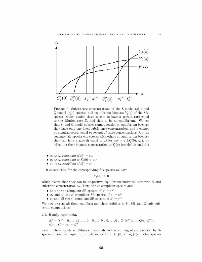
MICROORGANISM COMPETITION: EXCLUSION AND COEXISTENCE 15
Figure 5. Subsistence concentrations of the S-model (sx⋆i ) and
Q-model (sz⋆k ) species, and equilibrium biomass Yj(s) of the SB-
species, which enable these species to have a growth rate equalto the dilution rate D, and thus to be at equilibrium. We seethat S- and Q-model species cannot coexist at equilibrium becausethey have only one fixed subsistence concentration, and s cannotbe simultaneously equal to several of these concentrations. On thecontrary, SB-species can coexist with others at equilibrium becausethey can have a growth equal to D for any s ∈ [Sy
j (0), sin), by
adjusting their biomass concentration to Yj(s) (see definition (16))
• xi is s0-compliant if sx∗i = s0;
• yj is s0-compliant is Sj(0) < s0;• zk is s0-compliant if sz∗
k = s0
It ensues that, for the corresponding SB-species we have
Yj(s0) > 0
which means that they can be at positive equilibrium under dilution rate D andsubstrate concentration s0. Thus, the s⋆-compliant species are:
• only the s⋆-compliant SB-species, if s⋆ = sy⋆
• x1 and all the s⋆-compliant SB-species, if s⋆ = sx⋆
• z1 and all the s⋆-compliant SB-species, if s⋆ = sz⋆
We now present all these equilibria and their stability in S-, SB- and Q-only sub-strate competitions.
2.5. S-only equilibria.
Exi = (sx⋆
i , 0, . . . , x⋆i , . . . , 0 , 0, . . . , 0 , 0, . . . , 0 , Q1(s
x⋆i ), . . . , QNz
(sx⋆i ))
with x⋆i = sin − sx⋆
i
each of these S-only equilibria corresponds to the winning of competition by S-species i; such an equilibrium only exists for i ∈ {0, · · · , nx} (all other species
98

16 PIERRE MASCI, FREDERIC GROGNARD, ERIC BENOIT AND OLIVIER BERNARD
cannot survive at a substrate level lower than Sin fot the given D). In a compe-tition between several S-species, eqilibrium Ex
1 (with lowest substrate subsistenceconcentration sx⋆
1 ) is asymptotically globally stable, while all the others are unstable[1].
2.6. Q-only equilibria.
Ezk = (sz⋆
k , 0, . . . , 0 , 0, . . . , 0 , 0, . . . , z⋆k, . . . , 0 , Q1(s
z⋆k ), . . . , QNz
(sz⋆k ))
with z⋆k =
sin−sz⋆k
Qk(sz⋆k
)
Similarly to S-only equilibria, each of these Q-only equilibria corerspond to thewinning of competition by Q-species k; such an equilibrium only exists for k ∈{0, · · · , nz}. In a competition between several Q-species, eqilibrium Ez
1 (with lowestsubstrate subsistence concentration sz⋆
1 ) is asymptotically globally stable, while allthe others are unstable [2].
2.7. SB-only equilibria. We denominate G a subset of {1, · · · , ny} representingany SB-species coexistence. For example if we want to speak about species 1, 5 and7 coexistence, then we use G = {1, 5, 7}. We then define Ey
G the equilibrium wherethese species coexist. It is composed by
• sy⋆G such that sy⋆
G +∑
j∈G Yj(sy⋆G ) = sin because of (8)
• ∀j ∈ G, yj = Yj(sy⋆)
• for any other j, yj = 0• ∀i ∈ {1, · · · , Nx}, xi = 0• ∀k ∈ {1, · · · , Nz}, zk = 0• ∀k ∈ {1, · · · , Nz}), qk = Qk(sy⋆
G )
there exist many EyG equilibria, corresponding to all the possible G subset. The
globally asymptotically stable equilibrium of a competition with only SB-species isgiven by the choice G = {1, · · · , ny} [7]. Note that some of the G species can have anull biomass on these equilibria, as Yj(s
y⋆G ) might be null for some j ∈ G. Therefore
EyG1
and EyG2
with G1 6= G2 are not necessarily different.We must here introduce a technical hypothesis which will be useful later to prove
hyperbolicity of the equilibria.
Hypothesis 7. For all G and all j : Sj(0) 6= sy⋆G
2.8. Coexistence equilibria. As previously said in this section, there also existequilibria where one of the S- or Q-species coexist with several sx⋆
i - or sz⋆k -compliant
SB-species. For a coexistence with S-species we denote them E(x,y)⋆i,G . They are
composed of:
• s = sx⋆i
• ∀j ∈ G, yj = Yj(sx⋆i )
• for any other j, yj = 0• ∀l 6= i, xl = 0• ∀k ∈ {1, · · · , Nz}, zk = 0• ∀k ∈ {1, · · · , Nz}, qk = Qk(sx⋆
i )• xi = sin − sx⋆
i −∑
j∈G Yj(sx⋆i ) (this value will be denoted xG
i )
Similarly, for a coexistence with Q-species we denote them E(z,y)⋆k,G . They are
composed of:
• s = sz⋆k
• ∀j ∈ G, yj = Yj(sz⋆k )
99

MICROORGANISM COMPETITION: EXCLUSION AND COEXISTENCE 17
• for any other j, yj = 0• ∀i ∈ {1, · · · , Nx}, xi = 0• ∀l 6= k, zl = 0• ∀l ∈ {1, · · · , Nz}, ql = Ql(s
z⋆k )
• zk =sin−sz⋆
k −P
j∈G Yj(sz⋆k )
Qk(sz⋆k
) (this value will be denoted zGk )
To our knowledge, these equilibria have never been studied until now.Note that some of these equilibria might be reduntant with S- or Q-only equilib-
ria, if all the SB-species represented by G are not sx⋆i - or sz⋆
k -compliant. Note alsothat all those equilibria do not necessarily exist in the non-negative orthant. In-deed, xG
i and zGk can be negative, depending on sin and on the substrate subsistence
concentrations. These equilibria with negative components will not be studied anyfurther since we only consider initial conditions in the positive orthant, which isinvariant. In the sequel, we will denote E an equilibrium of (7) which belongs toan unspecified class.
We will now show that if s = s⋆ at equilibrium, there exists a positive equilibriumcontaining all s⋆-compliant species.
Lemma 2.8.
• If s⋆ = sx⋆ then E(x,y)⋆1,{1,··· ,ny}
is in the positive orthant.
• If s⋆ = sy⋆ then Ey⋆
{1,··· ,ny}is in the positive orthant.
• If s⋆ = sz⋆ then E(z,y)⋆1,{1,··· ,ny}
is in the positive orthant.
Proof. • If s⋆ = sx⋆, then all yj = Yj(sx⋆) ≥ 0 at equilibrium and sy⋆ +
∑ny
j=1 Yj(sy⋆) = sin implies that sx⋆ +
∑ny
j=1 Yj(sx⋆) < sin since sx⋆ < sy⋆ and
Yj(s) is non-decreasing. It directly follows that x⋆1 = sin−sx⋆−
∑ny
j Yj(sx⋆) >
0.• If s⋆ = sy⋆, then all xi and zk are zero at equilibrium and all yj = Yj(s
y⋆) ≥ 0• If s⋆ = sz⋆, then all yj = Yj(s
z⋆) ≥ 0 at equilibrium and sy⋆ +∑ny
j=1 Yj(sy⋆) =
sin implies that sz⋆ +∑ny
j=1 Yj(sz⋆) < sin since sz⋆ < sy⋆. It directly follows
that z⋆1 =
sin−sz⋆−Pnz
jYj(s
z⋆)
Qk(sz⋆) > 0.
We call E⋆ the equilibrium with all s⋆-compliant species remaining in the chemo-stat, while all the others are excluded. Depending on the species subsistence con-centrations, E⋆ can be one of the previously presented equilibria:
• if s⋆ = sy⋆ then E⋆ = Ey⋆
{1,··· ,ny}: only the s⋆-compliant SB-species remain in
the chemostat.• if s⋆ = sx⋆ then E⋆ = E
(x,y)⋆1,{1,··· ,ny}
: the best S-species (lowest sx⋆i ) remains in
the chemostat with all the sx⋆i -compliant SB-species.
• if s⋆ = sz⋆ then E⋆ = E(z,y)⋆1,{1,··· ,ny}
: the best Q-species (lowest sz⋆k ) remains in
the chemostat with all the sz⋆k -compliant SB-species.
In the next section, we present an important global stability result for this equilib-rium.
3. Statement and demonstration of the Main Theorem: competitive ex-clusion or coexistence in the generalized competition model. This theorem
100
18 PIERRE MASCI, FREDERIC GROGNARD, ERIC BENOIT AND OLIVIER BERNARD
states that all the s⋆-compliant species (those who can be at equilibrium with sub-strate subistence concentration s⋆, which is the lowest of all sx⋆.sy⋆, sz⋆) coexist inthe chemostat at equilibrium, while all the others are excluded.
Main Theorem. In the generalized competition model (7), if Hypotheses 1–7hold, then all the solutions of the system, having xi(0), yj(0), zk(0) > 0 for alls∗-compliant species, converge asymptotically towards equilibrium E⋆.
Structure of the proof: In a first step we reduce system (7) to the mass balancesurface. Then we present a non decreasing lower bound L(t) for s(t), and use itto demonstrate that s converges towards s⋆. Finally only the s∗-compliant specieshave a large enough substrate concentration to remain in the chemostat, so thatall other S-, Q-, and SB-model species are washed out. The final step consists inshowing that the convergence result that we showed on the mass-balance surfacecan be extended to the whole non-negative orthant.
Remark 3. It is not restrictive to consider xi(0), yj(0), zk(0) > 0 for the solutionsof the system since species with null initial condition can be ignored, so that we canthen consider a smaller dimensional system.
3.1. Step 1: we consider the system on the mass balance surface andin the region where qk ∈ (Q0
k, Qmk ) for all k ∈ {1, ..., Nz}. Lemma 2.5 indi-
cates that qk reaches (Q0k, Qm
k ) in finite time, and in (8) we showed that the totalconcentration of intra and extracellular substrate in the chemostat M converges tosin.
We denote ”Σ”, the generalized competition model (7) on the mass balancesurface defined by
M = s +
Nx∑
i=1
xi +
Ny∑
j=1
yj +
Nz∑
k=1
qkzk = sin (25)
For the remainder of the demonstration we will study system Σ, and we willlater show that its asymptotic convergence towards an equilibrium has the samebehaviour as the initial model (7). While studying system Σ, we will howeverretain all the states of the original system and the expressions of the equilibria; Σis then defined by the addition of the invariant constraint (25).
3.2. Step 2: we propose a non decreasing lower bound L(t) for s. The mainobstacle for the demonstration of the Main Theorem was the possibility that s wouldrepeatedly be lower than s⋆ and repeatedly be higher than s⋆
n = max(sx∗nx
, sz∗nz
),which would generate an oscillating behaviour. In order to eliminate this possibilitywe build a non decreasing lower bound for s, which converges towards s⋆
1. We nowpresent such a lower bound, which will be used to show that s converges to s⋆ inthe next sections.
Lemma 3.1. In system Σ
L(t) = min
(
mink
(Szk(qk(t))),min
j(Sy
j (yj(t)), s⋆, s(t)
)
is a non decreasing lower bound for s
Proof. We know that the right derivative of L is the derivative of one of the functionwhich realizes the minimum. In four cases we show that this right derivative is nonnegative.
101

MICROORGANISM COMPETITION: EXCLUSION AND COEXISTENCE 19
• Case 1: If Szk(qk(t)) realizes the minimum then its derivative is non negative,
because Szk(qk) goes towards s (see (15)).
• Case 2: If Syj (yj(t)) realizes the minimum then its derivative is non negative,
because Syj (s) goes towards s (see (20)).
• Case 3: If s(t) realizes the minimum then we examine its dynamics s forsystem Σ (i.e. on the mass balance equilibrium manifold). We replace sin bys +
∑
i xi +∑
j yj +∑
k qkzk:
s =∑
i
(D − αi(s))xi +∑
j
(D − βj(s, yj))yj +∑
k
(Dqk − ρk(s)) zk
which is equivalent to, from the definition (11) of Qk(s) :
s =∑
i
(D − αi(s))xi +∑
j
(D − βj(s, yj))yj +∑
k
(Dqk − γk(Qk(s))Qk(s)) zk
Then– for all i, s ≤ s⋆ gives us αi(s) ≤ D, so that the first sum is non negative;– for all j, s ≤ Sy
j (yj)) gives us βj(s, yj) ≤ βj(Syj (yj), yj) = D), so that the
second sum is non negative;– for all k, s ≤ Sz
k(qk) gives us Qk(s) ≤ qk, and s ≤ s⋆ gives us γk(Qk(s)) ≤γk(Qk(sz⋆
k )) = D so that the third sum is also non negative.Finally we obtain
s ≥ 0
• Case 4: If s⋆ realizes the minimum, we know that its right derivative is nulland thus non negative.
3.3. Step 3: we demonstrate that s converges towards s⋆.
Lemma 3.2. In system Σ
limt→+∞
s(t) = s⋆
Proof. We first show, by contradiction, that the substrate concentration s(t) can-not converge towards any constant value other than s⋆. Suppose the reverse hy-pothesis, i.e. limt→+∞ s(t) = s 6= s⋆. Through Lemma 2.6, we then have thatlimt→+∞ qk(t) = Qk(s) and limt→+∞ yj(t) = Yj(s).
If s < s⋆,
• αi(s) < D for all i so that all xi go to 0• γk(Qk(s)) < D for all k implies that all zk go to 0
So that we have a contradiction with mass balance equilibrium (25), as the total
substrate (in the medium + in the biomasses) at equilibrium s +∑Ny
j=1 Yj(s) will
be lower than sy⋆ +∑Ny
j=1 Yj(sy⋆) = sin.
If s > s⋆ we must consider three cases:
• if s⋆ = sx⋆1 then αi(s) > D implies that x1 diverges to +∞, which is in
contradiction with the boundedness shown in (9).• if s⋆ = sz⋆
1 then γ1(Q1(s)) > D implies that z1 diverges to +∞, which is incontradiction with the boundedness shown in (10).
• if s⋆ = sy⋆ then we have a contradiction with mass balance equilibrium (25),
because s +∑Ny
j=1 Yj(s) will be higher than sy⋆ +∑Ny
j=1 Yj(sy⋆) ≤ sin.
102
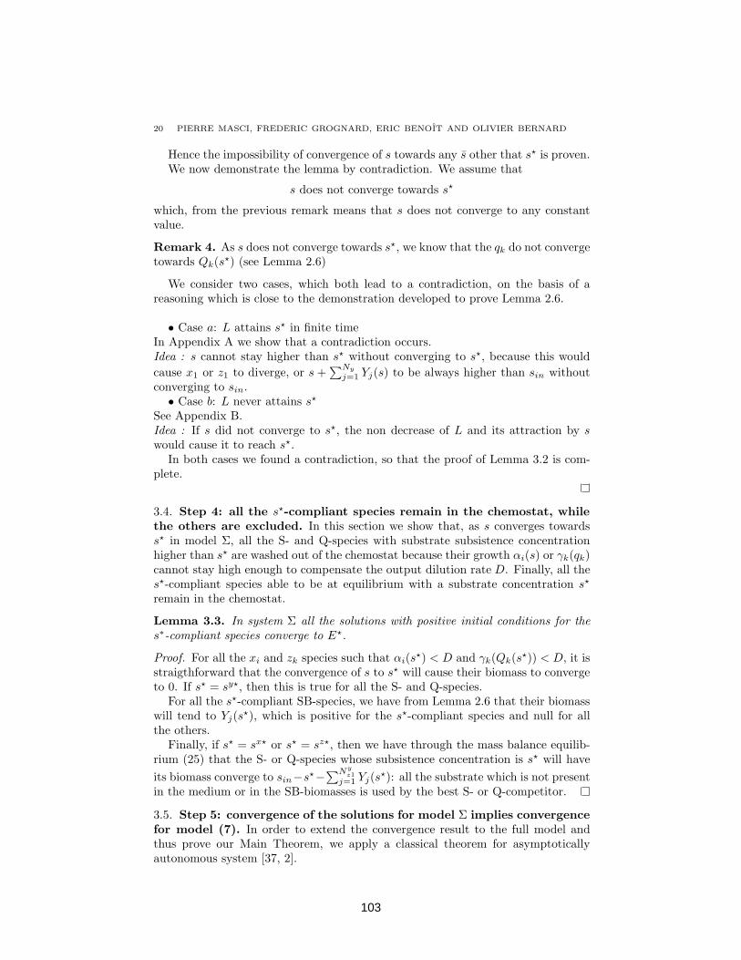
20 PIERRE MASCI, FREDERIC GROGNARD, ERIC BENOIT AND OLIVIER BERNARD
Hence the impossibility of convergence of s towards any s other that s⋆ is proven.We now demonstrate the lemma by contradiction. We assume that
s does not converge towards s⋆
which, from the previous remark means that s does not converge to any constantvalue.
Remark 4. As s does not converge towards s⋆, we know that the qk do not convergetowards Qk(s⋆) (see Lemma 2.6)
We consider two cases, which both lead to a contradiction, on the basis of areasoning which is close to the demonstration developed to prove Lemma 2.6.
• Case a: L attains s⋆ in finite timeIn Appendix A we show that a contradiction occurs.Idea : s cannot stay higher than s⋆ without converging to s⋆, because this would
cause x1 or z1 to diverge, or s +∑Ny
j=1 Yj(s) to be always higher than sin withoutconverging to sin.
• Case b: L never attains s⋆
See Appendix B.Idea : If s did not converge to s⋆, the non decrease of L and its attraction by swould cause it to reach s⋆.
In both cases we found a contradiction, so that the proof of Lemma 3.2 is com-plete.
3.4. Step 4: all the s⋆-compliant species remain in the chemostat, whilethe others are excluded. In this section we show that, as s converges towardss⋆ in model Σ, all the S- and Q-species with substrate subsistence concentrationhigher than s⋆ are washed out of the chemostat because their growth αi(s) or γk(qk)cannot stay high enough to compensate the output dilution rate D. Finally, all thes⋆-compliant species able to be at equilibrium with a substrate concentration s⋆
remain in the chemostat.
Lemma 3.3. In system Σ all the solutions with positive initial conditions for thes∗-compliant species converge to E⋆.
Proof. For all the xi and zk species such that αi(s⋆) < D and γk(Qk(s⋆)) < D, it is
straigthforward that the convergence of s to s⋆ will cause their biomass to convergeto 0. If s⋆ = sy⋆, then this is true for all the S- and Q-species.
For all the s⋆-compliant SB-species, we have from Lemma 2.6 that their biomasswill tend to Yj(s
⋆), which is positive for the s⋆-compliant species and null for allthe others.
Finally, if s⋆ = sx⋆ or s⋆ = sz⋆, then we have through the mass balance equilib-rium (25) that the S- or Q-species whose subsistence concentration is s⋆ will have
its biomass converge to sin−s⋆−∑N
yz1
j=1 Yj(s⋆): all the substrate which is not present
in the medium or in the SB-biomasses is used by the best S- or Q-competitor.
3.5. Step 5: convergence of the solutions for model Σ implies convergencefor model (7). In order to extend the convergence result to the full model andthus prove our Main Theorem, we apply a classical theorem for asymptoticallyautonomous system [37, 2].
103

MICROORGANISM COMPETITION: EXCLUSION AND COEXISTENCE 21
Lemma 3.4. All solutions of system (7) with positive initial conditions for thes∗-compliant species converge to E∗ defined in section 2.7.
Remark 5. While, up to here, we simply had considered Σ as the same systemas (7), in the same dimension, except that it was restricted to (25), we will nowequivalently explicitely include (25) into system (7) to obtain Σ in the form of asystem that has one dimension less than (7) by omitting the s coordinate. Sinceboth representations of Σ are equivalent, the previously proven stability resultsare still valid in the new representation, with the exception that convergence takesplace towards equilibria directly derived from these presented in sections 2.5-2.8 byomitting the s coordinate. These new equilibria are differentiated from the originalones by adding a ˜ , so that an arbitrary equilibrium is denoted E.
Proof. System Σ can be written as follows :
xi =
αi
sin −
Nx∑
l=1
xl −
Ny∑
m=1
ym −
Nz∑
r=1
qrzr
− D
xi
yj =
βj
sin −
Nx∑
l=1
xl −
Ny∑
m=1
ym −
Nz∑
r=1
qrzr, yj
− D
yj
zk = (γk(qk) − D)zk
qk = ρk
sin −
Nx∑
l=1
xl −
Ny∑
m=1
ym −
Nz∑
r=1
qrzr
− fk(qk)
for i ∈ {1, · · · , Nx}, j ∈ {1, · · · , Ny}, k ∈ {1, · · · , Nz}
(26)
where the s state has been removed compared to (7). In order to recover model (7),we should add the equation
M = D(sin − M)
which we interconnect with (26) by replacing every sin in (26) with M . It is thisinterconnection that we will now study.
In the first part of the proof, we will show that every solution of (7) convergesto an equilibrium E. We will then show by induction that all the solutions that donot converge to E∗ have an initial condition with some xi = 0, yj = 0 or zk = 0 forsome s∗-compliant species. Thus, all the solutions with xi 6= 0, yj 6= 0, zk 6= 0 forthe s∗-compliant species converge to E∗.
For that, we will use Theorem F.1 from [2]. We will therefore first compute thestable manifolds of all equilibria of Σ:
• The stable manifold of E∗ is of dimension Nx +Ny +2Nz. It is constituted ofall the initial conditions which verify xi(0), yj(0), zk(0) > 0 for s∗-compliantspecies and xi(0), yj(0), zk(0) ≥ 0 for all other species, as well as qk ≥ 0 forall k (see Lemma 3.3).
• The stable manifold of E0 is of dimension Nx −nx +Ny −ny +2Nz −nz. It isconstitued of all the initial conditions which verify x1(0) = . . . = xnx
(0) = 0,y1(0) = . . . = yny
(0) = 0 and z1(0) = . . . = znz(0) = 0. The only species
that can be present at the initial condition are those that cannot survivefor the given D and sin. Indeed, if any xi(0) > 0 for i ≤ nx (or similaryj(0) > 0 or zk(0) > 0), one can apply Lemma 3.3. to the reduced ordersystem containing these species to show that convergence does not take place
104

22 PIERRE MASCI, FREDERIC GROGNARD, ERIC BENOIT AND OLIVIER BERNARD
towards E0. Conversely, any initial condition with x1(0) = . . . = xnx(0) = 0,
y1(0) = . . . = yny(0) = 0 and z1(0) = . . . = znx
(0) = 0 generates a solution
that goes to E0 since for the other species we have:– xi < (αi(sin) − D)xi, with αi(sin) − D < 0 for all i > nx because of the
definition of nx presented in (23);– yj < (βj(sin, yj) − D)yj , with βj(sin, 0) − D < 0 for all j > ny, because
of the definition of ny;– zk < (γk(Qk(sin)) − D)zk, with γk(Qk(sin)) − D) < 0 for all k > nz
because of the definition of nz.• The dimension of the stable manifold of any other E can be computed from
Lemma 3.3. To an equilibrium E corresponds a substrate value s (> s∗ bydefinition of s∗). Lemma 3.3 indicates that solutions of Σ converge towards anequilibrium corresponding to s, if there is no smaller subsistance concentrationcorresponding to a species present in the system (for S- and Q species) and ifall S-, Q- and SB-species that are s-compliant are present in the correspondingequilibrium. The stable manifold of E must therefore be constrained to initialconditions that verify xi(0) = 0, yj(0) = 0 and zk(0) = 0 for all species that
are s-compliant for some s ≤ s and that are not positive in E. Having set allthese values to zero, it is indeed clear that s is the s⋆ as defined in Lemma3.3 of the reduced order system (without the aforementionned xi, yj and zk
coordinates). All solutions defined in Lemma 3.3 of this system then converge
to E, which justifies our definition of the stable manifold of E. Its dimensionis Nx +Ny +2Nz −nE,s, where nE,s is the number of s-compliant species (for
some s ≤ s) that are not present in E.
Through Lemma 3.3, we have in fact shown that all solutions of Σ in the non-negative orthant converge to an equilibrium. Indeed, for a given initial condition,either it belongs to the stable manifold of E0 or, eliminating from the system allspecies that are null at the initial time necessarily sets it in a form where Lemma3.3 can be applied (which shows convergence to an equilibrium).
The dimension of the stable manifold of any equilibrium E will therefore be theone of E plus 1. The hypotheses of Theorem F.1 from [2] are indeed all verified:
• The whole system (7) is bounded (see section 2.1)• The equilibria of system Σ are hyperbolic (see Appendix C.2-C.6).• There are no cycles of equilibria in system Σ. Indeed, if we analyze the
potential transition between two equilibria, both equilibria must belong tothe same face, so that convergence takes place to the one corresponding tothe smallest value of s. A potential sequence of equilibria would then becharacterized by a decreasing value of s at each equilibrium, which preventsit from cycling.
We can then conclude from this theorem that all solutions of (7) tend to an equi-librium. We are then left with checking to what equilibrium they tend.
Before continuing this proof, we need to detail nE,s. In the case of E = E∗ and
s = s∗, we have nE,s = 0 (by definition, all s∗-compliant species are present in E∗
and there is no other species that is compliant for smaller values of s). Otherwise,we necessarily have nE,s > 0. Indeed, we know that s > s∗, so that all species
present in E∗ are compliant for some s < s; as such, in order to have nE,s = 0, E
would need to at least contain all species that are present in E∗. In such a case no
105

MICROORGANISM COMPETITION: EXCLUSION AND COEXISTENCE 23
S and Q species can be present in E∗ (otherwise, it could not be present in E alsofor a different value of s). Defining J the set of SB-species that are present in E∗
and writing (25) for E∗ then yields
M = s∗ +∑
j ∈ J
Yj(s∗) = sin
Equality (25) should also be valid in s > s∗ so that
sin = s +
Nx∑
i=1
xi +
Ny∑
j=1
yj +
Nz∑
k=1
qkzk > s +∑
j ∈ J
Yj(s) > sin
where we have the last inequality (which leads to a contradiction) because Yj(s) is
an increasing function. We can then conclude that, for all E 6= E∗, nE,s > 0, andat least one s⋆-compliant species species must be null.
In order to check to what equilibrium solutions of (7) tend, we use an inductionargument, by supposing that our Main Theorem has been proven up to N − 1species, which we use for the proof for N species. Along with the fact that thestability result is trivial for 1 species (classical Monod model, [2], classical Droopmodel, [21] and generalized Contois model, [7]), this will conclude our proof.
Let us consider a system of N species with equilibrium E∗ as defined earlier.This equilibrium contains positive species (which are s⋆-compliant) and null species(which are not s⋆-compliant).
Imposing, for one of the not s⋆-compliant species, xi = 0 (or yj = 0 or zk = 0) forthe initial condition, sets us in the framework where we have N − 1 species presentin the system. Also, since this species did not belong to the positive ones in E⋆, itsabsence does not change anything into which equilibrium is the one correspondingto the smallest subsistance concentration, which remains E⋆. We can then applythe induction hypothesis, which indicates that all such initial conditions initiatesolutions that converge to E⋆ (as long as the s⋆-compliant species have positiveinitial condition).
Studying now the equilibrium E0, we know from the beginning of the proof thatits stable manifold is of dimension Nx−nx+Ny−ny +2Nz−nz +1. As was done forΣ, it is directly apparent that any initial condition with x1(0) = . . . = xnx
(0) = 0,y1(0) = . . . = yny
(0) = 0 and z1(0) = . . . = znx(0) = 0 generates a solution that has
all species exponentially go to zero. Finally, the analysis of the s equation showsthat it has the form s = D(sin − s)−F (t) with F (t) exponentially going to zero sothat s goes to sin and all such solutions go to E0.
We can now consider all the other equilibria. Let an equilibrium E correspondingto a substrate concentration s (> s∗ by definition). As we have seen in our analysis
of Σ, the stable manifold of the corresponding E is of dimension Nx+Ny+2Nz−nE,s,so that the stable manifold of E is of dimension Nx +Ny +2Nz−nE,s +1. Let us setourselfes in the situation where all nE,s species are set to zero at the initial time andall others are positive. We can then consider the system with only the remainingNx +Ny +2Nz −nE,s positive species and the substrate. We have seen that, in this
case, all solutions of the corresponding reduced order Σ go to E which means thats is the “s∗” defined in Lemma 3.4 for the reduced order system. Since the reducedorder system contains less than N species because nE,s > 0, we conclude that all
solutions of the full system (7) that have zero initial condition for all nE,s species
and positive values for all Nx +Ny +2Nz−nE,s others converge to E. We have then
106

24 PIERRE MASCI, FREDERIC GROGNARD, ERIC BENOIT AND OLIVIER BERNARD
exhibited an invariant manifold of dimension Nx + Ny + 2Nz − nE,s + 1 for whichall solutions go to E; this corresponds to the predicted dimension of the stablemanifoldof E. No solution with some of the nE,s species positive (among which
there is at least on s∗-compliant species) at the initial time can then converge to E.This completes the proof of our Main Theorem since all solutions go to an equi-
librium and we have exhibited the stable manifold of all equilibria other thanE∗. These manifolds cannot go into the region where xi, yj or zk > 0 for alls ∗ −compliant species because at least one of them is in the corresponding nE,s-set. All initial conditions in the region where xi, yj or zk > 0 for all s ∗−compliantspecies therefore generate solutions that go to E∗.
4. Discussion: How D and sin both determine competition outcome. InS- and Q-only competitions, the outcome of competition is mainly determined byD, which fixes the sx⋆
i and sz⋆k S- and Q-substrate subsistence concentrations; the
role of sin is to allow the best competitor (already determined by the value of D)to settle the reactor, or to cause it to be washed out with all the others. On thecontrary in SB-only competition, both controls have important roles: D fixes theYj(s) functions, while sin determines the equilibrium, where sy⋆+
∑
j Yj(sy⋆) = sin.
With a low enough sin, only few SB-species will settle the chemostat (sy⋆ being lowin this case, there will be few sy⋆-compliant species, with non-null Yj(s
y⋆)), whereasa high enough sin can enable all SB-species to coexist.
Finally, in a mixed S-Q-SB-competition the dilution rate D fixes all the S- andQ-substrate subsistence concentrations sx⋆
i and sz⋆k , as well as the Yj(s) functions,
while the input substrate concentration sin selects the species remaining in thereactor, by limiting the available nutrients, and thus the biomasses present in thereactor at equilibrium. Figure 6 gives an example between three competitors.
On this figure the sx⋆ and sz⋆ values and the Y (s) function are fixed by D. Heresz⋆1 is lower than sx⋆
1 , so that the S-species will be outcompeted and washed out.Then the value of sin determines wether
1. no species remain at equilibrium2. only the SB-species remains at equilibrium, as there is not enough input sub-
strate to feed both SB- and Q-species: because sy⋆ + Y (sy⋆) = sin andsin < sz⋆ + Y (sz⋆), we know that sy⋆ < sz⋆, so that s⋆ = sy⋆, and onlythe SB-species remains in the reactor.
3. both the SB- and Q-species remain in the chemostat: here sin > sz⋆ +Y (sz⋆)and sin = sy⋆ + Y (sy⋆) give sy⋆ > sz⋆, so that s⋆ = sz⋆ and the Q-speciesremains in the reactor, coexisting with the sz⋆-compliant SB-species.
In this last case D has fixed the sz⋆ substrate equilibrium value and the Y (s)function, and at equilibrium the total substrate in the chemostat, equal to sin, willbe composed of
• the substrate in the medium sz⋆ (which is fixed by D and does not depend onsin);
• the SB-species internal substrate Y (sz⋆) (which is also fixed by D only);• the Q-species internal substrate Q(sz⋆))z⋆ = sin−Y (sz⋆)−sz⋆, which depends
on sin.
By going from left to right in Figure 6, starting with sin = 0, it is possible toimagine the input substrate concentration increase, thus enabeling more and moresubstrate s = sin at equilibrium (zone 1). Then in zone 2 the SB-species is present
107
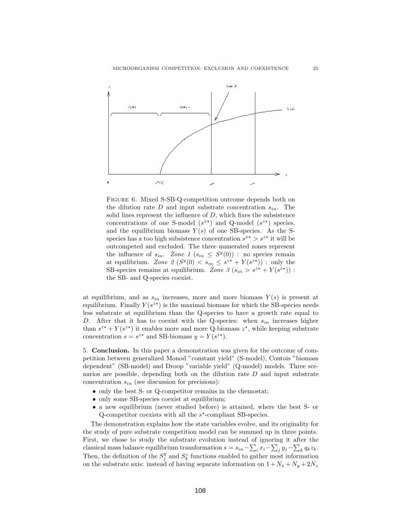
MICROORGANISM COMPETITION: EXCLUSION AND COEXISTENCE 25
Figure 6. Mixed S-SB-Q-competition outcome depends both onthe dilution rate D and input substrate concentration sin. Thesolid lines represent the influence of D, which fixes the subsistenceconcentrations of one S-model (sx⋆) and Q-model (sz⋆) species,and the equilibrium biomass Y (s) of one SB-species. As the S-species has a too high subsistence concentration sx⋆ > sz⋆ it will beoutcompeted and excluded. The three numerated zones representthe influence of sin. Zone 1 (sin ≤ Sy(0)) : no species remainat equilibrium. Zone 2 (Sy(0) < sin ≤ sz⋆ + Y (sz⋆)) : only theSB-species remains at equilibrium. Zone 3 (sin > sz⋆ + Y (sz⋆)) :the SB- and Q-species coexist.
at equilibrium, and as sin increases, more and more biomass Y (s) is present atequilibrium. Finally Y (sz⋆) is the maximal biomass for which the SB-species needsless substrate at equilibrium than the Q-species to have a growth rate equal toD. After that it has to coexist with the Q-species: when sin increases higherthan sz⋆ + Y (sz⋆) it enables more and more Q-biomass z⋆, while keeping substrateconcentration s = sz⋆ and SB-biomass y = Y (sz⋆).
5. Conclusion. In this paper a demonstration was given for the outcome of com-petition between generalized Monod ”constant yield” (S-model), Contois ”biomassdependent” (SB-model) and Droop ”variable yield” (Q-model) models. Three sce-narios are possible, depending both on the dilution rate D and input substrateconcentration sin (see discussion for precisions):
• only the best S- or Q-competitor remains in the chemostat;• only some SB-species coexist at equilibrium;• a new equilibrium (never studied before) is attained, where the best S- or
Q-competitor coexists with all the s⋆-compliant SB-species.
The demonstration explains how the state variables evolve, and its originality forthe study of pure substrate competition model can be summed up in three points.First, we chose to study the substrate evolution instead of ignoring it after theclassical mass balance equilibrium transformation s = sin−
∑
i xi−∑
j yj−∑
k qkzk.
Then, the definition of the Syj and Sz
k functions enabled to gather most informationon the substrate axis: instead of having separate information on 1+Nx +Ny +2Nz
108
26 PIERRE MASCI, FREDERIC GROGNARD, ERIC BENOIT AND OLIVIER BERNARD
axes we obtained a one dimensional view on these dynamics (Figure 2 and 3),where all the Sy
j (yj) and Szk(qk) go towards s. We have thus turned a complex
1 + Nx + Ny + 2Nz dimensional problem into a simpler one: ”how do s and theSy
j (yj) and Szk(qk) behave on the substrate axis, and what are the consequences for
the biomasses?”.Finally the definition of the non decreasing lower bound L(t) (section 3.2) and itsconvergence towards s⋆ (section 3.3) were the last steps for this demonstration toemerge.
Monod and Droop-only pure competitions for substrate lead to the ”survival ofthe fittest”, the fittest being the species with lowest substrate requirement s⋆. Onthe contrary, Contois-only competition lead to a coexistence equilibrium, becausebiomass dependence gives SB-species the capability to remain at equilibrium fordifferent substrate concentrations in the range [Sy
j (0), sin) (see Figure 5). Monodand Droop species are mutually exclusive, which leads to the pessimization principleof adaptative dynamics [38] : ”mutation and natural selection lead to a deteriorationof the environmental condition, a Verlenderung. We end up with the worst of allpossible environment.” On the contrary Contois species are coexistence-compliantthanks to biomass dependence, which nuances the pessimization principle: ”somespecies could live in worse environments (s = minj(S
yj (0)) being the worse one) but
if there is enough substrate for other species, they can coexist.” (see Figure 6 anddiscussion)
Since the introduction of the concept of evolution, with its link to competitiveexclusion [8] and the ”paradox of phytoplankton” [12] modelling has tried to ap-prehend competition, and to predict or control it. Our contribution in this frame-work was to extend the results proven in the N-species Monod model, N-speciesDroop model and N-species Contois model, where the outcome of competition waspredicted and explained with mathematical arguments, accompanied by ecologicalinterpretations.
Appendix A. Step 3 - Case a: L attains s⋆ in finite time. In this case
• if s⋆ = sz⋆1 we consider Figure 7 where L attains s⋆ after a finite time tL:
∀t ≥ tL, L(t) = s⋆1
Substep 3a.1: after a finite time larger than tL, q1 is repeatedly higher thanQ1(s
⋆) + θ. Since mini(Szk(qk)) ≥ L, we know that
∀t > tL, q1(t) ≥ Q1(s⋆)
As s does not converge to s⋆, we also know from Lemma 2.6 that q1 does notconverge towards Q1(s
⋆):
∃θ > 0,∀t > 0,∃tq > t, |q1(tq) − Q1(s
⋆)| > θ
Those two facts imply that the repeated exits of q1(t) from the θ-intervalaround Q1(s
⋆) take place above Q1(s⋆) for any tq > tL, so that, in that case,
we have q1(tq) > Q1(s
⋆)+θ. In Figure 7, such tq time instants are representedby •.
109
MICROORGANISM COMPETITION: EXCLUSION AND COEXISTENCE 27
Figure 7. Visual explanation of the demonstration of Lemma 3.2 -Case 1: L attains s⋆ in finite time tL (Q-model). i) q1 is repeatedlyhigher than Q1(s
⋆) + θ (•). ii) Because q1 is upper bounded byρm1 , so that q1 is higher than Q1(s
⋆) + θ/2 during non negligibletime intervals (dashed lines represent q1 = ρm
1 ). Thus z1 diverges,which is a contradiction.
Substep 3a.2: q1 is higher than Q1(s⋆) + θ/2 during non negligible time inter-
vals. Since the q1-dynamics are upper bounded with
q1 ≤ ρm1
we know that every time q1 is higher than Q1(s⋆)+ θ, it has been higher than
Q1(s⋆) + θ/2 during a time interval of minimal duration A(θ) = θ
2ρm1
. On
Figure 7, q1 = ρm1 is represented by the dashed lines.
Substep 3a.3: then z1 diverges, which is impossible. From time tL on, we havethat q1 ≥ Q1(s
⋆) ⇒ γ1(q1) ≥ D, so that z1(t) is non decreasing. During eachof the time interval where q1 is higher than Q1(s
⋆) + θ/2, the increase of z1 islower bounded by
z1 = γ1(Q1(s⋆) + θ/2) − D = C(θ) > 0
so that every tq time we have
z1(tq) − z1(t
q − A(θ)) > C(θ)A(θ)
As such increases occurs repeatedly, and as z1 is non decreasing, z1 diverges.This is a contradiction because z1 is upper bounded (see (10)).
• if s⋆ = sx⋆1 then the non convergence of s to s⋆, and the fact that s ≥ s⋆ will
cause s to be non negligibly ”away” from s⋆, so that x1 will diverge, causinga contradiction with (9). This is exactly the same demonstration as above (inthe case s⋆ = sz⋆
1 ) without needing the qk study.
• if s⋆ = sy⋆ then s +∑Ny
j=1 Yj(s) will always be higher than sin = sy⋆ +∑Ny
j=1 Yj(sy⋆) without converging to sin, which is in contradiction with (25).
110

28 PIERRE MASCI, FREDERIC GROGNARD, ERIC BENOIT AND OLIVIER BERNARD
Appendix B. Step 3 - Case b: L never attains s⋆. In this case L(t) converges
towards a value L ∈ (0, s⋆], because it is non decreasing and bounded in [0, s⋆], sothat
∀ǫ > 0,∃tL(ǫ) > 0,∀t > tL(ǫ), |L(t) − L| < ǫ
We consider the neighborhood of L in Figure 8.
Figure 8. Visual explanation of the demonstration of Lemma 3.2- Case 2: L never attains s⋆. i) s is repeatedly higher than L + λ(•). ii) s is upper bounded by Dsin, so that s is higher than
L+λ/2 during non negligible time intervals (dashed lines represents = Dsin) iii) during such a time intervals L = mink(Sz
k(qk)) (orminj(S
yj (yj))) is increasing non negligibly towards s, so that L
cannot both converge towards L and stay lower than L during thewhole time interval: there is a contradiction.
Substep 3b.1: after a finite time, s is repeatedly higher than L + λ. Since, from thebeginning of the proof of Lemma 3.2, we know that s does not converge to anyconstant value, hence not to L,
∃λ > 0,∀t > 0,∃ts > t, |s(ts) − L| > λ
Since L is increasing and converges to L, it reaches L − λ in finite time tL(λ).
After this finite time, s is higher than L + λ on every ts time instants, which arerepresented by • in Figure 8.
Substep 3b.2: s is higher than L+λ/2 during non negligible time intervals. Becauseof the boundedness of s
s ≤ Dsin
every time s is higher than L + λ, it has been higher than L + λ/2 during a nonnegligible time interval of minimal duration A(λ) = λ
2Dsin. On Figure 8 the case
s = Dsin is represented by dashed lines.
111
MICROORGANISM COMPETITION: EXCLUSION AND COEXISTENCE 29
Substep 3b.3: L = mink(Szk(qk)) (or minj(S
yj (yj))) is increasing non negligibly
towards s, so that L cannot both converge towards L and stay lower than L duringthe whole time interval: there is a contradiction. Like in previous proofs, we areinterested in what happens during the [ts−A(λ), ts] time-interval, with ts−A(λ) >
tL(ǫ) (for some ǫ < λ). Since, during this time-interval, s(t) > L + λ/2 and L < L,
we know that there exists a k such that L(ts) = Szk(qk(ts)) < L, or a j such that
L(ts) = Syj (yj(t
s)) < L.
For both this step (3b.3) we choose to first only present arguments for the caseL(ts) = mink(Sz
k(qk)); almost similar arguments for the case L(ts) = minj(Syj (yj))
will then be briefly presented.
• if L(ts) = mink(Szk(qk)), then during the whole considered time-interval, as
Szk(qk) was increasing, we know that
L − ǫ < L ≤ Szk(qk) ≤ Sz
k(qk(ts)) < L (27)
so that Qk(L− ǫ) < qk(t) < Qk(L). For the k species, the dynamics of qk canthen be lower bounded:
qk ≥ ρk(L + λ/2) − fk(Qk(L))
and then
qk ≥ ρk(L + λ/2) − ρk(L) = Gk(λ)
positive, so that the increase of qk during the [ts − A(λ), ts] time-interval isalso lower bounded:
qk(ts) − qk(ts − A(λ)) ≥ Gk(λ)A(λ) = Hk(λ)
Since Qk = Sz−1
k is locally Lipschitz with constant K (because f ′k > 0), we
have
qk(ts) − qk(ts − A(λ)) = Qk(Szk(qk(ts))) − Qk(Sz
k(qk(ts − A(λ))))< K [Sz
k(qk(ts)) − Szk(qk(ts − A(λ)))]
so that the corresponding increase of Szk(qk) is lower bounded with
Szk(qk(ts)) − Sz
k(qk(ts − A(λ))) ≥ 1K
Hk(λ)
and then
Szk(qk(ts − A(λ))) < L −
1
KHk(λ)
which implies the same higher bound for L:
L(ts − A(λ)) < L −1
KHk(λ)
By choosing ǫ < 1K
Hk(λ), this inequality is contradictory with (27) so thatCase 2 is not possible
• if L(ts) = minj(Syj (yj)), then the same arguments can be developped for the
j species, with a lower bound Gj(λ) on the yj dynamics:
Gj(λ) = βj(L + λ/2, Yj(L)) − βj(L, Yj(L)) > 0
and then an increase of variable yj at least equal to Hj(λ) = Gj(λ)A(λ)followed by a non negligible increase of L
L(ts − A(λ)) < L −1
KHj(λ)
112
30 PIERRE MASCI, FREDERIC GROGNARD, ERIC BENOIT AND OLIVIER BERNARD
because Yj is locally Lipschitz. Finally a contradiction also occurs when ǫ <1K
Hj(λ):
L(ts − A(λ)) < L − ǫ
Appendix C. Computation of system Σ Jacobian Matrix and eigenvaluesfor all the equilibria. Computation of the Jacobian Matrix of system Σ, with
s = sin −∑Nx
i=1 xi −∑Ny
j=1 yj −∑Nz
k=1 qkzk.
Jxx Jxy Jxz Jxq
Jyx Jyy Jyz Jyq
Jzx Jzy Jzz Jzq
Jqx Jqy Jqz Jqq
where
Jxxii = αi(s) − D − ∂αi
∂sxi and ∀l 6= i, Jxx
il = −∂αi
∂sxi
Jxyij = −∂αi
∂sxi
Jxzik = −∂αi
∂sxiqk
Jxqik = −∂αi
∂sxizk
and
Jyxji = −
∂βj
∂syj
Jyyjj = βj(s, yj) − D +
∂βj
∂yjyj −
∂βj
∂syj and ∀l 6= j, Jyy
jl = −∂βj
∂syj
Jyzjk = −
∂βj
∂syjqk
Jyqjk = −
∂βj
∂syjzk
andJzx
ki = 0Jzy
kj = 0
Jzzkk = γk(qk) − D and ∀l 6= k, Jzz
kl = 0
Jzqkk = ∂γk
∂qkzk and ∀l 6= k, Jzq
kl = 0
and
Jqxki = −∂ρk
∂s
Jqykj = −∂ρk
∂s
Jqzkl = −∂ρk
∂sql
Jqqkk = −∂ρk
∂szk − ∂fk
∂qkand ∀l 6= k, Jqq
kl = −∂ρk
∂szl
Fortunately for eigenvalue computations, at equilibria the null biomasses willsimplify the matrix:
• when xi = 0, then the whole ith line gives eigenvalue αi(s) − D (denoted”xi-eigenvalue”) and can be deleted, as well as the ithcolumn;
• when yj = 0 then the whole Nx+jth line gives eigenvalue βj(s, yj)−D (denoted”yj-eigenvalue”) and can be deleted, as well as the Nx + jth correspondingcolumn;
• when zk = 0 then the whole Nx + Ny + kth line gives eigenvalue γk(qk) − D(denoted ”zk-eigenvalue”) and can be deleted, as well as the Nx + Ny + kth
column; in a second step, the whole Nx + Ny + Nz + kth column can also be
deleted and gives eigenvalue −∂fk
∂qk(denoted ”qk-eigenvalue”), as well as the
Nx + Ny + Nz + kth line.
113

MICROORGANISM COMPETITION: EXCLUSION AND COEXISTENCE 31
C.1. Complete washout equilibrium. With this in hand, we see that for equi-librium E0 (xi = yj = zk = 0) the Jacobian matrix is triangular, so that theeigenvalues lay on the diagonal. They are:
• αi(sin) − D• βj(sin, 0) − D• γk(Qk(sin)) − D
• −∂fk
∂qk(negatives)
We denote nx, ny, nz the number of S-, SB- and Q- species verifying the inequalitiesof Hypothesis 5, and thus having the possibility to be at equilibrium with a positivebiomass, under controls D and sin. Each of these species has a positive correspond-ing eigenvalue on this equilibrium, so that equilibirum E0 has nx +ny +nz positiveeigenvalues, and Nx − nx + Ny − ny + 2Nz − nz negative eigenvalues.
C.2. S-only equilibria. For equilibrium Exi we get all the previously cited x-,y-,
z-and q-eigenvalues:
• αl(sx⋆i ) − D whose signs are the same as sign(sx⋆
i − sx⋆l )
• βj(sx⋆i , 0)−D which are positive if the jth species is sx⋆
i -compliant, or negativeelse;
• γk(Qk(sx⋆i )) − D whose signs are the same as sign(sx⋆
i − sz⋆k )
• −∂fk
∂qkwhich are all negative
and the remaining eigenvalue corresponds to the positive xi-only dynamics:
xi = (αi(sin − xi) − D)xi
which yields the eigenvalue −∂αi
∂sx⋆
i for S-species i. Each S- or Q-species witha substrate subsistence concentration sx⋆
l or sz⋆k lower than sx⋆
i gives a positiveeigenvalue. Among all the Ex
i equilibria, only Ex1 is stable if and only if s⋆ = sx⋆
1 <sz⋆1 , and if all the SB-species are not sx⋆
1 -compliant.
C.3. Q-only equilibria. For Equilibrium Ezk we get all the
• x-eigenvalues whose signs are the sign of sign(sz⋆k − sx⋆
i );• y-eigenvalues: as previously, y-eigenvalues are positive if the corresponding
SB-species is sz⋆k -compliant and negative else;
• zl-eigenvalues whose signs are the sign of sign(sz⋆k − sz⋆
l );• ql-eigenvalues for all l 6= k (negative);
and the remaining eigenvalues correspond to the positive (zk, qk)-only dynamics:{
zk = (γk(qk) − D)zk
qk = ρk(sin − qkzk) − fk(qk)
and we obtain the following resulting matrix:(
0 ∂γk
∂qkzk
−∂ρk
∂sqk −∂ρk
∂szk − ∂fk
∂qk
)
which has negative trace and positive determinant, so that its two eigenvalues arereal negative. Just like before, each S- or Q-species with a substrate subsistenceconcentration sx⋆
i or sz⋆l lower than sz⋆
k gives a positive eigenvalue. Among all theEz
k equilibria, only Ez1 is stable if and only if s⋆ = sz⋆
1 < sx⋆1 , and if all the SB-species
are not sz⋆1 -compliant.
114

32 PIERRE MASCI, FREDERIC GROGNARD, ERIC BENOIT AND OLIVIER BERNARD
C.4. SB-only equilibria. Now let us consider the EyG equilibria for which all j ∈ G
(where G represents a subset of {1, . . . , Ny}) SB-species coexist in the chemostatunder substrate concentration sy⋆
G , while all the S- and Q-species are washed out.sy⋆
G is defined by sy⋆G +
∑
j∈G Yj(sy⋆G ) = sin. Note that some of the G species can
have a null biomass on these equilibria, as Yj(sy⋆G ) might be null for some j ∈ G.
This gives all the
• x-eigenvalues whose sign are the same as the signs of sx⋆i − sy⋆
G ;• z-eigenvalues whose sign are the same as the signs of sz⋆
k − sy⋆G ;
• q-eigenvalues (negative).
All the yj species who are not included in G give negative eigenvalues if they arenot sy⋆
G -compliant, and positive eigenvalues else; their eigenvalues cannot be nullbecause of technical hypothesis 7. All the yj species who are included in G buthave a null biomass Yj(s
y⋆G ) on the Ey
G equilibrium give negative eigenvalues. Nowlet us study the remaining matrix Jyy
G which is composed of all the j ∈ G lines ofJyy, for which Yj(s
y⋆G ) > 0, and thus βj(s
y⋆G , Yj(s
y⋆G )) = D:
yj =
(
βj(s −∑
l
yl, yj) − D
)
yj
which yields the Jacobian matrix:
JyyG =
−a1 − b1 . . . −a1 . . . −a1
.... . .
......
−aj . . . −aj − bj . . . −aj
......
. . ....
−an . . . −an . . . −an − bn
with aj =∂βj
∂sYj(s
y⋆G ) > 0 and bj = −
∂βj
∂yjYj(s
y⋆G ) > 0.
Let us show that this matrix has only real negative eigenvalues, by using thedefinition of an eigenvalue λ = (A + Bi), where A ∈ R is the real part and B ∈ R
the imaginary part:
JyyG ·
y1
...yn
= (A + Bi)
y1
...yn
(28)
We obtain n equations:
−bjyj − aj
∑
l
yl = (A + Bi)yj
and thus
(A + Bi + bj)yj = −aj
∑
l
yl (29)
If we have A + Bi + bj = 0 for some j, then B = 0 and A = −bj < 0 so that wehave a negative eigenvalue.Else, isolating yj yields
yj =−aj
∑
l yl
bj + A + Bi
115
MICROORGANISM COMPETITION: EXCLUSION AND COEXISTENCE 33
Summing over j, we obtain
∑
j
yj =∑
j
(
−aj
∑
l yl
bj + A + Bi
)
Now if∑
j yj = 0, since some yj must be different of 0, (29) yields, for that j, thatA + Bi + bj = 0 so that again B = 0 and A = −bj < 0.Else, simplifying the sums of yl and yj , this yields
1 =∑
j
(
−aj
bj+A+Bi
)
=∑
j
(
−aj(bj+A−Bi)(bj+A)2+B2
)
=∑
j
(
−aj(bj+A)(bj+A)2+B2
)
+ i∑
j
(
ajB)(bj+A)2+B2
)
Since the left-hand-side is real, the imaginary part of the right-hand side must bezero, which imposes B = 0. For thr right-hand-side to be positive, at least one ofthe bj + A must be negative, which translates into minj(bj + A) < 0 and
A < −minj
bj < 0
We conclude from this that all eigenvalues of this matrix are real negative.Finally, an Ey
G equilibrium is stable if and only if all the SB-species not containedin G are not sy⋆
G -compliant (this is equivalent to saying that sy⋆G = sy⋆, with sy⋆ =
sy⋆
{1,...,Ny}), and if s⋆ = sy⋆.
C.5. S-coexistive equilibria. In this section we consider equilibria E(x,y)i,G where
S-species xi coexists with the SB-species in G, a subset of {1, . . . , Ny}, under sub-strate concentration sx⋆
i .We obtain here all the
• xl-eigenvalues (l 6= i) whose signs are the signs of sx⋆i − sx⋆
l ;• z-eigenvalues whose sign is the sign of sx⋆
i − sz⋆k ;
• q-eigenvalues (negative);
yj-eigenvalues with j not in G are positive if yj is sx⋆i -compliant and negative else;
yj-eigenvalues with j in G but have a null biomass Yj(sx⋆i ) give negative eigenvalues.
For the remaining SB-species, and species xi, we obtain the following system:{
xi = (αi(sin − xi −∑
l yl) − D)xi
yj = (βj(sin − xi −∑
l yl, yj) − D) yj
and the Jacobian matrix:
−a0 −a0 . . . −a0 . . . −a0
−a1 −a1 − b1 . . . −a1 . . . −a1
......
. . ....
...−aj −aj . . . −aj − bj . . . −aj
......
.... . .
...−an −an . . . −an . . . −an − bn
with a0 = ∂αi
∂sx⋆
i > 0, aj =∂βj
∂sYj(s
x⋆i ) > 0 and bj = −
∂βj
∂yjYj(s
x⋆i ) > 0 (for
j ∈ {1, · · · , n}). This matrix has exactly the same form has the one considered onAppendix C.4. The only difference being that the there is no “b0” in the first element
116
34 PIERRE MASCI, FREDERIC GROGNARD, ERIC BENOIT AND OLIVIER BERNARD
of the matrix. Defining a b0 = 0, we can then conclude that all eigenvalues are realand negative because, following the development of Appendix C.4, we obtain
A < −minj
bj = 0
Finally, only equilibrium E(x,y)1,{1,...,Ny}
can be stable if and only if s⋆ = sx⋆1 .
C.6. Q-coexistive equilibria. In this section we consider equilibria E(z,y)k,G where
Q-species zk coexists with the SB-species in G, a subset of {1, . . . , Ny}, undersubstrate concentration sz⋆
k .We obtain here all the
• x-eigenvalues whose signs are the signs of sz⋆k − sx⋆
i ;• zl-eigenvalues (l 6= j) whose sign are the signs of sz⋆
k − sz⋆l ;
• q-eigenvalues (negative);
yj-eigenvalues with j not in G are positive if yj is sz⋆k -compliant and negative else;
yj-eigenvalues with j in G but have a null biomass Yj(sz⋆k ) give negative eigenvalues.
For the remaining SB-species, and species zk, we obtain the following model
yj = (βj(sin −∑
l yl − qkzk, yj) − D)yj
zk = (γk(qk) − D)zk
qk = ρk(sin −∑
l yl − qkzk) − fk(qk)
and, swapping the last two equations and using fk(qk) = γk(qk)qk, we get theJacobian matrix:
−a1 − b1 . . . −a1 . . . −a1 −a1zk −a1qk
.... . .
......
......
−aj . . . −aj − bj . . . −aj −ajzk −ajqk
......
. . ....
...−an . . . −an . . . −an − bn −anzk −anqk
−an+1 . . . −an+1 . . . −an+1 −an+1zk − bn+1qk − γ −an+1qk
0 . . . 0 . . . 0 bn+1zk 0
with aj =∂βj
∂sYj(s
z⋆k ) > 0 and bj = −
∂βj
∂yjYj(s
z⋆k ) > 0 for j ∈ {1, · · · , n}, with
an+1 = ∂ρk
∂sand bn+1 = ∂γk
∂qk. By using the definition of eigenvalue λ = (A + Bi)
(see (28)) we follow a similar path to that of Appendix C.4, we show that theeigenvalues are real and negative.
Finally, only equilibrium E(z,y)1,{1,...,Ny}
can be stable if and only if s⋆ = sz⋆1 .
Remark 6. The same work can be done for the whole system (7), where theeigenvalues are the same, plus the −D eigenvalue which arises from mass balancedynamics (8).
REFERENCES
[1] R. Armstrong, R. McGehee, Competitive exclusion, American Naturalist 115 (1980) 151.[2] H. Smith, P. Waltman, The theory of the chemostat. Dynamics of microbial competition,
Cambridge Studies in Mathematical Biology. Cambridge University Press, 1995.[3] S. Hsu, T. Hsu, Competitive exclusion of microbial species for a single-nutrient with internal
storage, SIAM Journal on Applied Mathematics 68 (6) (2008) 1600–1617.[4] D. Tilman, R. Sterner, Invasions of equilibria: tests of resource competition using two species
of algae, Oecologia 61 (2) (1984) 197–200.
117

MICROORGANISM COMPETITION: EXCLUSION AND COEXISTENCE 35
[5] S. Hansen, S. Hubell, Single-nutrient microbial competition: qualitative agreement betweenexperimental and theoretically forecast outcomes, Science 207 (4438) (1980) 1491–1493.
[6] D. Tilman, Resource competition between plankton algae: An experimental and theoreticalapproach., Ecology 58 (22) (1977) 338–348.
[7] F. Grognard, F. Mazenc, A. Rapaport, Polytopic lyapunov functions for persistence analysis ofcompeting species, Discrete and Continuous Dynamical Systems-Series B 8 (1) (2007) 73–93.
[8] G. Hardin, The competitive exclusion principle, Science 131 (3409) (1960) 1292–1297.[9] C. Elton, Animal Ecology, Sidgwick & Jackson, LTD. London, 1927.
[10] C. Darwin, On the Origin of Species by Means of Natural Selection, or the Preservation ofFavoured Races in the Struggle for Life, John Murray, 1859.
[11] M. Scriven, Explanation and prediction in evolutionnary theory, Science 130 (3374) (1959)477–482.
[12] G. E. Hutchinson, The paradox of the plankton, The American Naturalist 95 (1961) 137.[13] C. Jessup, S. Forde, B. Bohannan, Microbial experimental systems in ecology, Advances in
Ecological Research 37 (2005) 273–306.[14] G. Gause, The Struggle for Existence, Williams and Wilkins, Baltimore, 1934.[15] J. Monod, Reserches sur la croissance des cultures bacteriennes, Paris: Herrmann et Cie.[16] A. Sciandra, P. Ramani, The steady states of continuous cultures with low rates of medium
renewal per cell, J. Exp. Mar. Biol. Ecol. 178 (1994) 1–15.[17] M. Droop, Vitamin b12 and marine ecology, J. Mar. Biol Assoc. U.K. 48 (1968) 689–733.[18] J. Caperon, J. Meyer, Nitrogen-limited growth of marine phytoplankton. i. changes in popu-
lation characteristics with steady-state growth rate, Deep-Sea Res. 19 (1972) 601–618.
[19] I. Vatcheva, H. deJong, O. Bernard, N. Mars, Experiment selection for the discrimination ofsemi-quantitative models of dynamical systems, Artif. Intel. 170 (2006) 472–506.
[20] K. Lange, F. J. Oyarzun, The attractiveness of the Droop equations, Mathematical Biosciences111 (1992) 261–278.
[21] F. J. Oyarzun, K. Lange, The attractiveness of the Droop equations. II: Generic uptake andgrowth functions, Mathematical Biosciences 121 (1994) 127–139.
[22] O. Bernard, J.-L. Gouze, Transient behavior of biological loop models, with application tothe Droop model, Mathematical Biosciences 127 (1) (1995) 19–43.
[23] B. Haegeman, C. Lobry, J. Harmand, Modeling bacteria flocculation as density-dependent
growth, AICHE JOURNAL 53 (2) (2007) 535–539.[24] D. Contois, Kinetics of bacterial growth: relationship between population density and specific
growth rate of continuous cultures., J Gen Microbiol. (1959) 40–50.[25] J. Leon, D. Tumpson, Competition between two species of two complementary or substitutable
resources, J. Theor. Biol. 50 (1975) 185–201.[26] S. Hsu, K. Cheng, S. Hubbel, Exploitative competition of micro-organisms for two comple-
mentary nutrients in continuous culture, SIAM J. Appl. Math. 41 (1981) 422–444.[27] H. Freedman, J. So, P. Waltman, Coexistence in a model of competition in the chemostat
incorporating discrete delays, SIAM J. Appl. Math. 49 (1989) 859–870.[28] P. de Leenheer, H. Smith, Feedback control for the chemostat, J. Math. Biol. 46 (2003) 48–70.[29] P. de Leenheer, D. Angeli, A. Sontag, A feedback perspective for chemostat models with
crowding effects, in: Positive Systems, Vol. 294 of Lecture Notes in Control and Inform. Sci,Springer-Verlag, 2003, pp. 167–174.
[30] J. Arino, S. Pilyugin, G. Wolkowicz, Considerations on yield, nutrient uptake, cellular growth,and competition in chemostat models, Canadian Applied Math Quarterly 11 ((2003) [2005])107–142.
[31] J. B. Wilson, Mechanisms of species coexistence: twelve explanations for the hutchinson’s’paradox of the phytoplankton’: evidence from new zealand plant communities, New Zealandjournal of Ecology 17–42 (1990) 137.
[32] A. Fredrickson, G. Stephanopoulos, Microbial competition, Science 213 (1981) 972–979.[33] J. Gouze, G. Robledo, Feedback control for nonmonotone competition models in the chemo-
stat, Nonlinear Analysis: Real World Applications (2005) 671–690.
[34] P. de Leenheer, B. Li, H. Smith, Competition in the chemostat : some remarks, Canadianapplied mathematics quarterly 11 (2) (2003) 229–247.
[35] N. Rao, E. Roxin, Controled growth of competing species, Journal on Applied Mathematics50 (3) (1990) 853–864.
[36] P. Masci, O. Bernard, F. Grognard, Continuous selection of the fastest growing species in thechemostat, in: Proceedings of the IFAC conference, Seoul, Korea, 2008, pp. 9707–9712.
118

36 PIERRE MASCI, FREDERIC GROGNARD, ERIC BENOIT AND OLIVIER BERNARD
[37] H. R. Thieme, Convergence results and a Poicare-Bendixson trichotomy for asymptoticallyautonomous differential equations, Journal of Mathematical Biology 30 (7) (1992) 755–763.
[38] O. Diekmann, A beginner’s guide to adaptive dynamics, Banach Center Publ. (2003) 47–86.
Received September 2006; revised February 2007.
E-mail address: [email protected]
E-mail address: [email protected], [email protected],
119

Continuous Selection of the Fastest
Growing Species in the Chemostat
Pierre Masci, Olivier Bernard, and Frederic Grognard
INRIA- Project COMORE, 2004 route des lucioles, BP 93, 06902Sophia Antipolis Cedex, FRANCE
Tel : 0033.4.92.38.71.85; e-mail : [email protected],[email protected], [email protected]
Abstract: This paper proposes control laws for the continuous culture of microorganisms, whichmake it possible to select species which maximize a criterion. In particular, by controlling thedilution rate and the input substrate concentration, the species with the fastest growth rate inchosen environmental conditions can be selected.In a first step a control is proposed for Monod and Droop models in order to achieveperiodic substrate stresses, and a closed loop control is proposed to regulate the total biomassconcentration. We show that this biomass regulation causes the selection of the fastest growingspecies if the system has a periodic behavior, and derive new selection criteria. Finally, themethod is simulated using the Droop model for selecting species which maximize these criteria.
Keywords: chemostat; microorganisms; competition; selection
1. INTRODUCTION
The chemostat is an open bioreactor where a microorgan-ism can grow in suboptimal conditions of substrate limita-tion. The chemostat model supports several ecological the-ories (Jessup et al. [2005]) that were then extrapolated andtested in real life. Among these theories, the competitiontheory is one of the most famous. It states that if n compet-ing species are introduced in a chemostat, generically (inthe adequate working modes) only one species will stay inthe chemostat, while the n − 1 other will disappear. Thisprinciple was validated with real experiments in Hansenand Hubell [1980] where the species that ”wins” the com-petition could be predicted; it was the one that could growat a constant rate (equal to the dilution rate as detailedfurther on) with the smallest amount of limiting substrates∗. This theoretical result could be used to select amonga blend of species, the ones of interest. This idea has beenused for diverse applications, such as Directed Evolutionfor strain improvement (see the reviews of Dykhuizen andHartl [1983], Zelder and Hauer [2000] and Percival Zhanget al. [2006]). By adjusting a particular stress such as aninhibitor’s concentration, a substrate limitation, or thedilution rate, it can lead to the isolation of species withoptimal yield. This is of particular importance since it isa rather simple way of making a particular species emergewithin a population. However, in most biotechnologicalapplications, the selection criterion based on the idea of”optimal yield” is not appropriate. A selection that woulde.g. select the microorganism with the highest growthpotential would be preferable, especially if one wants toidentify organisms that grow in hostile conditions. Moregenerally, the objective of this paper is to propose newselection criteria. For this, the chemostat is not run inopen loop, but a control law is proposed to run the systemin closed loop. We show how the competition outcome is
modified and we propose new criteria that could be usedfor species separation.
The paper is structured as follows. In a first part we recalltwo classical models of microorganisms in the chemostat,and the classical competition principle. Then we proposecontrol laws to generate periodic substrate stresses, and toput the chemostat into a turbidostat mode. In the thirdpart we show that this last control causes the selection ofthe fastest growing species if the system has a periodicbehavior, and infer new selection criteria. A simulationexample illustrates the benefit of the approach and showshow three species can be separated on this principle.
2. SHORT REVIEW OF COMPETITION ON ASINGLE SUBSTRATE IN THE CHEMOSTAT
2.1 Basic model for microorganisms in the chemostat
Monod model is the basic model for describing microor-ganisms growth on a single substrate in a chemostat.
s = D(sin − s) −
N∑
i=1
1
yiµi(s)xi
xi = (µi(s) − D)xi
(1)
where s stands for the substrate concentration in thechemostat, sin its input concentration, and xi the ithspecies biomass concentration. The µi functions representthe growth rates of these species, and the yi constants aretheir substrate conversion yields. D is the input/outputdilution rate. We control the system with sin and D.
In this model the growth rate functions µi are taken aspositive monotonic increasing functions
sa < sb ⇔ µi(sa) < µi(sb) (2)
120

They are bounded by their supremum values µmi:
µi(s) < µmiand lim
s→+∞
µi(s) = µmi(3)
2.2 Variable yield model
Droop model (Droop [1968]) is more complex, it describesthe internal substrate storage q of the microorganisms :
s = D(sin − s) −
N∑
i=1
ρi(s)xi
qi = ρi(s) − µi(qi)qi
xi = (µi(qi) − D)xi
(4)
In this model the ρi functions represent the substrate ab-sorption rates, while the µi functions represent the growthrates. These functions are positive monotonic increasingfunctions. They are upper-bounded by the supremum val-ues ρmi
and µi. The minimum absorption and growth rateare ρi(0) = 0 and µi(qi) = 0 for qi ∈ [0, Kqi
].
Internal substrate storage behavior : For each fixed sub-strate concentration s, the qi equation indicates that qi
goes toward Qi(s), defined as the unique solution of
µi(Qi(s))Qi(s) = ρi(s) (5)
The uniqueness of Qi(s) and its attractivity for a fixed sare straightforward since µi(qi)qi is increasing in qi.
Let us define the maximum internal substrate storage
Qmi= lim
s→+∞
Qi(s) (6)
Qmiis thus the solution of µi(Qmi
)Qmi= ρmi
.
Qi(s) is bounded in [Kqi, Qmi
], and Kqiand Qmi
are lowerand upper-bounds for qi along the solutions of (4). Indeedfor qi(t) = Kqi
(resp. qi(t) = Qmi) then qi ≥ 0 (resp.
qi ≤ 0), so that the interval [Kqi, Qmi
] is invariant for qi.The fact that there is a minimum and a maximum internalsubstrate storage for each species is biologically relevant.
Corresponding to the maximum internal substrate storage,there is a maximum growth rate µmi
for each species
µmi= µi(Qmi
) (7)
2.3 The Competitive Exclusion Principle (CEP)
Under constant D and sin, for some xi species, there existsa substrate concentration s⋆
i for which the growth rate µi
at equilibrium is equal to the dilution rate D :
µi(s⋆i ) = D in the Monod model
µi(Qi(s⋆i )) = D in the Droop model
(8)
If this substrate concentration does not exist for a givenspecies, it means that µi(s) or µi(Qi(s)) < D ∀s, andthe species will be washed out of the chemostat. Ifµi(sin) or µi(Qi(sin)) < D for a particular species, thatspecies will also be washed out of the chemostat becausewe will have s(t) < sin after some finite time t0, and thenµi(s(t)) or µi(Qi(s(t))) < D for all t > t0.
With no loss of generality, we order the species so thattheir s⋆
i satisfy : s⋆1 < s⋆
2 < ... < s⋆N .
Hypothesis 1. s⋆1 < sin and x1(0) > 0
The CEP stipulates that in a chemostat with single sub-strate growth limitation, constant controls D and sin, andunder hypothesis 1, only species 1 stays in the chemostat:
limt→+∞
x1(t) > 0
∀i ∈ [2, N ], limt→+∞
xi(t) = 0(9)
Criterion 2. CEP’s Competitiveness CriterionUnder hypothesis 1, the species with smallest s⋆
i , whoneeds less substrate than the others for obtaining anequilibrium growth rate µi(s) or µi(Qi(s)) equal to thedilution rate D, wins the competition and excludes allothers from the chemostat.
Proof : A demonstration can be found in Smith andWaltman [1995] for the Monod model with N species andfor the Droop model with 2 species. It has been validatedwith several species (Hansen and Hubell [1980] - Ducobuet al. [1998]). 2
The CEP is crucial for the understanding of naturalecosystems. Some authors (Li and Smith [2003] - Hesseleret al. [2006] - Lobry and Harmand [2006]) developpedalternative models for which the CEP is not verified, inorder to explore some coexistence cases.
Motivations for this workSome works have already been done to control the compe-tition in the chemostat, generally to enable the coexistenceof several species (Rao and Roxin [1990] - de Leenheeret al. [2003] - Gouze and Robledo [2005]). Here we aim atfinding controls which change the result of the competitionkeeping a single species. More precisely, we want to selectspecies of interest who maximize a criterion other than thesmallest s⋆
i , by imposing a periodic behavior to the system.
Bernard et al. [1996] have studied the effect of periodicsubstrate stresses, which is a realistic ecological situation.In section 3.1 we propose controls which permit to repro-duce such stresses, and in section 4.3 we show that thiscan cause a new selection criterion.
3. CONTROLS FOR SELECTING SPECIES
3.1 Periodic substrate stresses
We propose an approach for the generation of periodicsubstrate stresses. It consists in periodically imposing aphase of rising substrate concentration, followed by a phaseof falling substrate concentration. The reference period isT = trise + tfall.
Rising phase during time trise
We choose sin to obtain the dynamics s = λ(sM − s) :
sin = s +1
D
(
λ(sM − s) +
N∑
i=1
ρi(s)xi
)
(10)
Control sin is positive because sM > s.
We obtain s(t) = sM (1 − e−λt) with s(0) = 0
Notice that∑N
i=1 ρi(s)xi is generally not available frommeasurements so that an observer may be built.
121
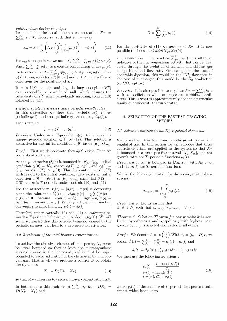
Falling phase during time tfall
Let us define the total biomass concentration XT =∑N
i=1 xi. We choose sin such that s = −γφ(s).
sin = s +1
D
(
XT
(
N∑
i=1
xi
XTρi(s)
)
− γφ(s)
)
(11)
For sin to be positive, we need XT
∑Ni=1
xi
XTρi(s) ≥ γφ(s).
Since∑N
i=1xi
XTρi(s) is a convex combination of the ρi(s),
we have for all s : XT
∑Ni=1
xi
XTρi(s) ≥ XT mini ρi(s). Then
φ(s) ≤ mini ρi(s) for s ∈ [0, sM ] and γ ≤ XT are sufficientconditions for the positivity of sin.
If γ is high enough and tfall is long enough, s(kT )can reasonably be considered null, which ensures theperiodicity of s(t) when periodically imposing control (10)followed by (11).
Periodic substrate stresses cause periodic growth ratesIn this subsection we show that periodic s(t) causesperiodic qi(t), and thus periodic growth rates µi(qi(t)).
Let us remind
qi = ρi(s) − µi(qi)qi (12)
Lemma 3. Under any T -periodic s(t), there exists aunique periodic solution qi(t) to (12). This solution isattractive for any initial condition qi(0) inside [Kqi
, Qmi]
Proof : First we demonstrate that qi(t) exists. Then weprove its attractivity.
As the qi-attractive Qi(s) is bounded in [Kqi, Qmi
], initialcondition qi(0) = Kqi
causes qi(T ) ≥ qi(0), and qi(0) =Qmi
causes qi(T ) ≤ qi(0). Thus by continuity of qi(T )with regard to the initial condition, there exists an initialcondition qi(0) = qi(0) in [Kqi
, Qmi] such that qi(T ) =
qi(0) and qi is T -periodic under controls (10) and (11)
For the attractivity, Vi(t) = |qi(t) − qi(t)| is decreasing
along the solutions : Vi(t) = sign(qi(t) − qi(t))(qi(t) −˙qi(t)) < 0 because sign(qi − ˙qi) = sign(−µi(qi)qi +µi(qi)qi) = −sign(qi − qi). Vi being a Lyapunov functionconverging to zero, limt→+∞ qi(t) = qi(t). 2
Therefore, under controls (10) and (11) qi converges to-wards a T -periodic behavior, and so does µi(qi(t)). We willsee in section 4.3 that this periodic behavior, caused by theperiodic stresses, can lead to a new selection criterion.
3.2 Regulation of the total biomass concentration
To achieve the effective selection of one species, XT mustbe lower bounded so that at least one microorganismsspecies remains in the chemostat, and it must be upperbounded to avoid saturation of the chemostat by microor-ganisms. That is why we propose a control D to obtainthe dynamics
XT = D(X⋆T − XT ) (13)
so that XT converges towards a chosen concentration X⋆T .
In both models this leads us to∑N
i=1 µi(.)xi − DXT =D(X⋆
T − XT ) and
D =
N∑
i=1
xi
X⋆T
µi(.) (14)
For the positivity of (11) we need γ ≤ XT . It is nowpossible to choose γ ≤ min(X⋆
T , XT (0)).
Implementation : In practice∑N
i=1 µi(.)xi is often anindicator of the microorganisms activity that can be mea-sured through the evolution of influent and effluent gascomposition and flow rate. For example in the case ofanaerobic digestion, this would be the CH4 flow rate; inthe case of microalgae, this would be the O2 production(or CO2 uptake).
Remark : It is also possible to regulate KT =∑N
i=1 kixi
with ki coefficients who can represent turbidity coeffi-cients. This is what is approximatively done in a particularfamily of chemostat, the turbidostat.
4. SELECTION OF THE FASTEST GROWINGSPECIES
4.1 Selection theorem in the XT -regulated chemostat
We have shown how to obtain periodic growth rates, andregulated XT . In this section we will suppose that thesecontrols or others are applied to the system so that XT
is bounded in a fixed positive interval [X0, Xm], and thegrowth rates are Ti-periodic functions µi(t).
Hypothesis 4. XT is bounded in [X0, Xm] with X0 > 0,and the µi(t) are Ti-periodic functions.
We use the following notation for the mean growth of thespecies :
µmeani=
1
Ti
Ti∫
0
µi(t)dt (15)
Hypothesis 5. Let us assume that∃j ∈ [1;N ] such that µmeanj
> µmeani∀i 6= j
Theorem 6. Selection Theorem for any periodic behaviorUnder hypotheses 4 and 5, species j with highest meangrowth µmeanj
is selected and excludes all others.
Proof : We denote di = ln(
xj
xi
)
.With xi = (µi −D)xi we
obtain di(t) =xj(t)xj(t)
− xi(t)xi(t)
= µj(t) − µi(t) and
di(t) = di(0) +∫ t
0µj(τ)dτ −
∫ t
0µi(τ)dτ
We then use the following notations :
pi(t) =t − mod(t, Ti)
Tiri(t) = mod(t, Ti)t = pi(t)Ti + ri(t)
(16)
where pi(t) is the number of Ti-periods for species i untiltime t. which leads us to
122

t∫
0
di(τ)dτ = pj(t)
Tj∫
0
µj(τ)dτ − pi(t)
Ti∫
0
µi(τ)dτ + Rji (t)
= pj(t)
Tj∫
0
µj(τ)dτ −pi(t)
pj(t)
Ti∫
0
µi(τ)dτ
+ Rji (t)
= pj(t)
(
Tjµmeanj−
pi(t)
pj(t)Tiµmeani
)
+ Rji (t)
with notation Rji (t) =
∫ rj(t)
0µj(τ)dτ −
∫ ri(t)
0µi(τ)dτ .
Since pi(t)pj(t)
= t−mod(t,Ti)
t−mod(t,Tj)
Tj
Ti, limt→+∞
pi(t)pj(t)
=Tj
Tiand
limt→+∞ di(t) = di(0)+pj(t)Tj
(
µmeanj− µmeani
)
+Rji (t).
Then as di(0) and Rji (t) are bounded, limt→+∞ di(t) =
+∞ because limt→+∞ pi(t) = +∞ and µmeanj> µmeani
.
Thus limt→+∞
xj(t)xi(t)
= +∞ and, as xj is upper bounded by
the upper-bound on XT , then limt→+∞ xi(t) = 0. As XT
is also lower bounded by X0 > 0, then lim inft→+∞ xj(t) ≥X0 > 0 and the proof is complete. 2
4.2 Selection of the species with highest µmi
We have shown that it is possible to select a species withfastest mean growth in given environmental conditions.Here we determine conditions for selecting the species withhighest µmi
. Bennett and Boraas [1988] have realized sucha selection by using a turbidostat culture.
Criterion 7. µmiSelection Criterion
With a bounded total biomass concentration XT , and withµi(t) ≈ µmi
∀t, the species with highest µmiis selected
Proof : The demonstration of Criterion 7 is the same asfor Theorem 6, with µmeani
= µmi. 2
Implementation : In order to have µi(t) ≈ µmi, we regu-
late s at a large value s0 (so that µi(s0) or µi(Qi(s0)) ≈µmi
) by imposing s = D(s0−s) which is achieved through
sin = s0 + 1D
∑Ni=1 ρi(s)xi.
Remark : From a practical point of view, as∑N
i=1 ρi(s)xi
is not always measurable, we have imagined a simpler wayto realize µi(s) or µi(Qi(s)) ≈ µmi
: with a high constantsin and a small X⋆
T we have s ≈ D(sin − s) and thesubstrate concentration will converge close to sin, which ischosen high enough to have µi(sin) or µi(Qi(sin)) ≈ µmi
.
4.3 Periodic stresses and new selection criterion
In this section we present the results that we obtained withcontrols (10), (11), and the Selection Theorem 6.
Functions used for the studyWe have used Michaelis-Menten absorption rates ρi(s) andDroop growth rates µi(qi) :
ρi(s) = ρmi
s
s + Ksi
µi(qi) = µi
(
1 −Kqi
qi
) (17)
Rectangular shaped stressesWith functions (17) and controls (10) and (11), we haveobtained pseudo-rectangular shaped stresses of Figure 1.
Fig. 1. Pseudo-rectangular shaped regular periodic stresses
The way to approach this regular rectangular shape asmuch as possible is described in section 5.
It is then reasonable (with sM ≫ Ksisuch that ρi(sM ) ≈
ρmi) to approximate the stresses by (18)
ρi(s(t)) =
{
ρmiif mod(t, T ) ≤ τ
0 if mod(t, T ) > τ(18)
The ratio τ/T is the proportion of time the microorgan-isms are fed, and (T−τ)/T is the proportion of time duringwhich they are stressed.
Determination of a new selection criterionUnder control (18) we have calculated the periodic be-havior of the internal substrate storage qi(t) presented inAppendix A, with limt→+∞ qi(t) = qi(t) (see Lemma 3)
We have then calculated :
µmeani=
1
T
µmi
µiln
1 +Qmi
/Kqi
1eµiτ
−1 +Qmi
/Kqi−1
eµiT−1
(19)
This criterion can be simplified in the specific case whereτ is small compared to T :
Hypothesis 8. τ/T ≪ 1Qmi
/Kqi−1 and τ ≪ 1
µi·Qmi/Kqi
Criterion 9. Selection Criterion under periodic stressesUnder control (18) and hypothesis 8, the species with
highest Tτ µmeani
≈ µmi
Qmi
Kqi
is selected.
whereQmi
Kqi
represents the capacity of the species to in-
crease its internal substrate storage.
Consequently, periodic stresses with a small τ make itpossible to select a species which can both grow fast andincrease significantly its internal substrate storage.
5. SIMULATIONS WITH THREE SPECIES
These simulations have been carried out on the Droopmodel (4) with control (14) so that the total biomassconcentration converges toward X⋆
T .
We have used (17) with the parameters of Table 1 for thespecies, whose values come from Vatcheva et al. [2006].
123
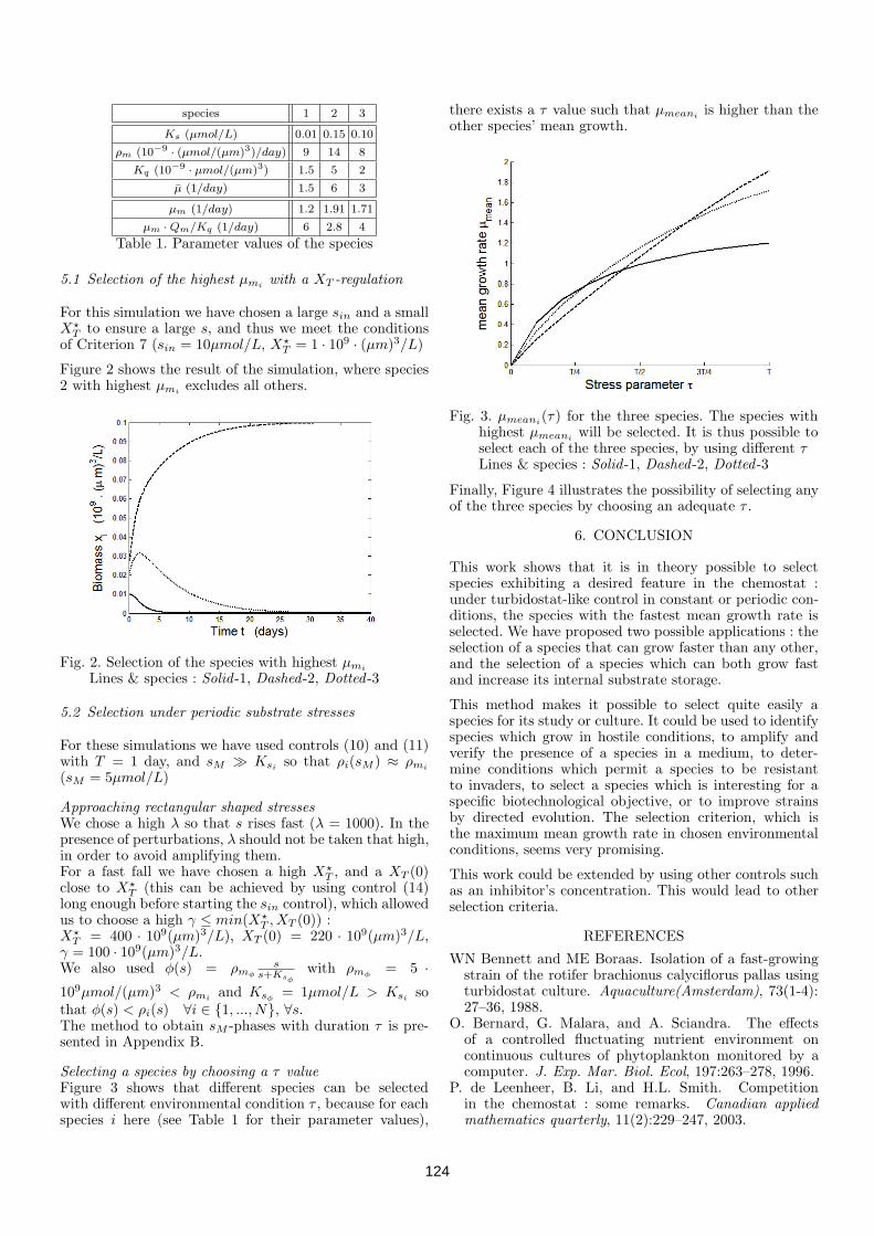
species 1 2 3
Ks (µmol/L) 0.01 0.15 0.10
ρm (10−9· (µmol/(µm)3)/day) 9 14 8
Kq (10−9· µmol/(µm)3) 1.5 5 2
µ (1/day) 1.5 6 3
µm (1/day) 1.2 1.91 1.71
µm · Qm/Kq (1/day) 6 2.8 4
Table 1. Parameter values of the species
5.1 Selection of the highest µmiwith a XT -regulation
For this simulation we have chosen a large sin and a smallX⋆
T to ensure a large s, and thus we meet the conditionsof Criterion 7 (sin = 10µmol/L, X⋆
T = 1 · 109 · (µm)3/L)
Figure 2 shows the result of the simulation, where species2 with highest µmi
excludes all others.
Fig. 2. Selection of the species with highest µmi
Lines & species : Solid-1, Dashed -2, Dotted -3
5.2 Selection under periodic substrate stresses
For these simulations we have used controls (10) and (11)with T = 1 day, and sM ≫ Ksi
so that ρi(sM ) ≈ ρmi
(sM = 5µmol/L)
Approaching rectangular shaped stressesWe chose a high λ so that s rises fast (λ = 1000). In thepresence of perturbations, λ should not be taken that high,in order to avoid amplifying them.For a fast fall we have chosen a high X⋆
T , and a XT (0)close to X⋆
T (this can be achieved by using control (14)long enough before starting the sin control), which allowedus to choose a high γ ≤ min(X⋆
T , XT (0)) :X⋆
T = 400 · 109(µm)3/L), XT (0) = 220 · 109(µm)3/L,γ = 100 · 109(µm)3/L.We also used φ(s) = ρmφ
ss+Ksφ
with ρmφ= 5 ·
109µmol/(µm)3 < ρmiand Ksφ
= 1µmol/L > Ksiso
that φ(s) < ρi(s) ∀i ∈ {1, ..., N}, ∀s.The method to obtain sM -phases with duration τ is pre-sented in Appendix B.
Selecting a species by choosing a τ valueFigure 3 shows that different species can be selectedwith different environmental condition τ , because for eachspecies i here (see Table 1 for their parameter values),
there exists a τ value such that µmeaniis higher than the
other species’ mean growth.
Fig. 3. µmeani(τ) for the three species. The species with
highest µmeaniwill be selected. It is thus possible to
select each of the three species, by using different τLines & species : Solid-1, Dashed -2, Dotted -3
Finally, Figure 4 illustrates the possibility of selecting anyof the three species by choosing an adequate τ .
6. CONCLUSION
This work shows that it is in theory possible to selectspecies exhibiting a desired feature in the chemostat :under turbidostat-like control in constant or periodic con-ditions, the species with the fastest mean growth rate isselected. We have proposed two possible applications : theselection of a species that can grow faster than any other,and the selection of a species which can both grow fastand increase its internal substrate storage.
This method makes it possible to select quite easily aspecies for its study or culture. It could be used to identifyspecies which grow in hostile conditions, to amplify andverify the presence of a species in a medium, to deter-mine conditions which permit a species to be resistantto invaders, to select a species which is interesting for aspecific biotechnological objective, or to improve strainsby directed evolution. The selection criterion, which isthe maximum mean growth rate in chosen environmentalconditions, seems very promising.
This work could be extended by using other controls suchas an inhibitor’s concentration. This would lead to otherselection criteria.
REFERENCES
WN Bennett and ME Boraas. Isolation of a fast-growingstrain of the rotifer brachionus calyciflorus pallas usingturbidostat culture. Aquaculture(Amsterdam), 73(1-4):27–36, 1988.
O. Bernard, G. Malara, and A. Sciandra. The effectsof a controlled fluctuating nutrient environment oncontinuous cultures of phytoplankton monitored by acomputer. J. Exp. Mar. Biol. Ecol, 197:263–278, 1996.
P. de Leenheer, B. Li, and H.L. Smith. Competitionin the chemostat : some remarks. Canadian appliedmathematics quarterly, 11(2):229–247, 2003.
124
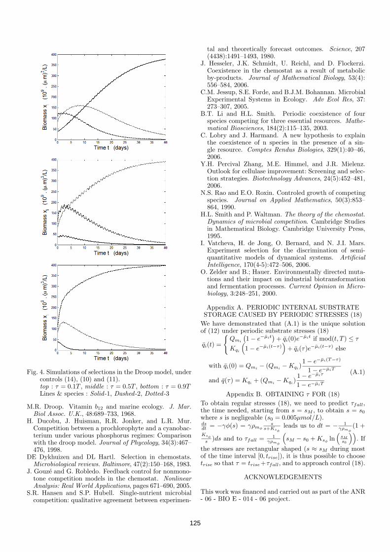
Fig. 4. Simulations of selections in the Droop model, undercontrols (14), (10) and (11).top : τ = 0.1T , middle : τ = 0.5T , bottom : τ = 0.9TLines & species : Solid-1, Dashed -2, Dotted -3
M.R. Droop. Vitamin b12 and marine ecology. J. Mar.Biol Assoc. U.K., 48:689–733, 1968.
H. Ducobu, J. Huisman, R.R. Jonker, and L.R. Mur.Competition between a prochlorophyte and a cyanobac-terium under various phosphorus regimes: Comparisonwith the droop model. Journal of Phycology, 34(3):467–476, 1998.
DE Dykhuizen and DL Hartl. Selection in chemostats.Microbiological reviews. Baltimore, 47(2):150–168, 1983.
J. Gouze and G. Robledo. Feedback control for nonmono-tone competition models in the chemostat. NonlinearAnalysis: Real World Applications, pages 671–690, 2005.
S.R. Hansen and S.P. Hubell. Single-nutrient microbialcompetition: qualitative agreement between experimen-
tal and theoretically forecast outcomes. Science, 207(4438):1491–1493, 1980.
J. Hesseler, J.K. Schmidt, U. Reichl, and D. Flockerzi.Coexistence in the chemostat as a result of metabolicby-products. Journal of Mathematical Biology, 53(4):556–584, 2006.
C.M. Jessup, S.E. Forde, and B.J.M. Bohannan. MicrobialExperimental Systems in Ecology. Adv Ecol Res, 37:273–307, 2005.
B.T. Li and H.L. Smith. Periodic coexistence of fourspecies competing for three essential resources. Mathe-matical Biosciences, 184(2):115–135, 2003.
C. Lobry and J. Harmand. A new hypothesis to explainthe coexistence of n species in the presence of a sin-gle resource. Comptes Rendus Biologies, 329(1):40–46,2006.
Y.H. Percival Zhang, M.E. Himmel, and J.R. Mielenz.Outlook for cellulase improvement: Screening and selec-tion strategies. Biotechnology Advances, 24(5):452–481,2006.
N.S. Rao and E.O. Roxin. Controled growth of competingspecies. Journal on Applied Mathematics, 50(3):853–864, 1990.
H.L. Smith and P. Waltman. The theory of the chemostat.Dynamics of microbial competition. Cambridge Studiesin Mathematical Biology. Cambridge University Press,1995.
I. Vatcheva, H. de Jong, O. Bernard, and N. J.I. Mars.Experiment selection for the discrimination of semi-quantitative models of dynamical systems. ArtificialIntelligence, 170(4-5):472–506, 2006.
O. Zelder and B.; Hauer. Environmentally directed muta-tions and their impact on industrial biotransformationand fermentation processes. Current Opinion in Micro-biology, 3:248–251, 2000.
Appendix A. PERIODIC INTERNAL SUBSTRATESTORAGE CAUSED BY PERIODIC STRESSES (18)
We have demonstrated that (A.1) is the unique solutionof (12) under periodic substrate stresses (18)
qi(t) =
{
Qmi
(
1 − e−µit)
+ qi(0)e−µit if mod(t, T ) ≤ τ
Kqi
(
1 − e−µi(t−τ))
+ qi(τ)e−µi(t−τ) else
with qi(0) = Qmi− (Qmi
− Kqi)1 − e−µi(T−τ)
1 − e−µiT
and q(τ) = Kqi+ (Qmi
− Kqi)1 − e−µiτ
1 − e−µiT
(A.1)
Appendix B. OBTAINING τ FOR (18)
To obtain regular stresses (18), we need to predict τfall,the time needed, starting from s = sM , to obtain s = s0
where s is negligeable (s0 = 0.005µmol/L).dsdt = −γφ(s) = γρmφ
ss+Ksφ
leads us to dt = − 1γρmφ
(1 +
Ksφ
s )ds and to τfall = 1γρmφ
(
sM − s0 + Ksφln(
sM
s0
))
. If
the stresses are rectangular shaped (s ≈ sM during mostof the time interval [0, trise]), it is thus possible to choosetrise so that τ = trise +τfall, and to approach control (18).
ACKNOWLEDGEMENTS
This work was financed and carried out as part of the ANR- 06 - BIO E - 014 - 06 project.
125

Driving competition in a complex ecosystem:
application to anaerobic digestion
P. Masci, O. Bernard, F. Grognard, E. Latrille and J.-B. Sorba and J.P. Steyer
Abstract— Anaerobic digestion is a wastewater treatmentprocess where bacteria degrade an organic substrate andproduce methane, which can be used as a biofuel. The firsttask when starting up an anaerobic digester is the increaseof its microbial population. It is a delicate phase, which isstill not well understood, and its influence on the digester’sfuture performance is not well known. During this phase, weshow that a competition between the various species occursand finally some species become dominant. In this paper,extending the competitive exclusion principle, we proposeto drive the competition during this start-up phase, byregulating the volatile fatty acids concentration, with the aimof selecting species with good performance in the standardoperating mode of the process. This new ”selective” start-upstrategy should lead to more efficient ecosystems.
Keywords: Anaerobic digestion; Bioreactors;Biological
systems; Competition; Selection; Directed Evolution
I. INTRODUCTION AND MOTIVATION
Anaerobic digestion is a more and more widely used
bioprocess for wastewater treatment. This complex ecosys-
tem involves several hundreds of bacterial and achaeal
species [1] that progressively degrade organic matter into
methane and CO2. It has many advantages compared
to the more widespread activated sludge process: it can
handle concentrated substrates, produces few sludge, and
methane can be recovered and used as a biofuel. However
this process is difficult to manage since the steady state
associated to the operating mode is not globally stable
[2]. As a corollary, the start-up of the digester is a long
and risky phase [3] during which the digester loading
is progressively increased in order to let the bacterial
population adapt, grow and settle the reactor. Reactor start-
up is then a long procedure (from one month to almost
one year) that is essential to achieve a high treatment
capacity at steady-state [4], and therefore this phase should
be better understood and controlled.
Despite its key role, this phase did not receive so far
much attention, perhaps because it is quite difficult to
properly characterise since biomass measurements are not
available. In [5], it was shown that disturbing the microbial
community in a ”bang bang” like approach leads to better
P. Masci, O. Bernard and F. Grognard are with INRIA SophiaAntipolis, 2004 route des lucioles, BP 93, 06902 Sophia Antipolis,France [email protected]
J.B. Sorba, E. Latrille and J.P. Steyer are with LBE, UR050, INRA,Avenue des etangs 11100 Narbonne, France
diversity and thus improves the bioprocess when facing a
toxicant.
In this paper, we propose a new model for the start-
up phase, including biodiversity. We assume that, at the
beginning, N species are competing for the substrate. We
show that, depending on the way the digester is started
up, some populations will be enhanced and will prefer-
entially remain in the digester. The underlying idea relies
on the competitive exclusion principle, which has been
theoretically studied and experimentally demonstrated in
various conditions [6], [7]. We exploit the idea proposed
in [8] to drive the competition during the start-up phase,
by regulating the volatile fatty acids (VFA) concentration
around a fixed value, which is determined by the normal
operating mode of the digester. By doing so, we act
upon the ecosystem in order to enhance the process
efficiency. Also, bacterial biomass extinction, which is one
of the main risks of the start-up phase, is avoided, and
the obtained ecosystem presents an interesting steadiness
property. Simulations and a first experiment are presented
for supporting this start-up strategy.
II. PROCESS MODELLING
A. Presentation of the model
We propose here a simple macroscopic model (derived
from [9]) in order to be able to handle the involved
mathematics. We assume that, in a first acidogenesis step,
the dissolved organic substrate, of concentration s1, is de-
graded by a population made of Na species of acidogenic
bacteria (yj , with j ∈ [1;Na]) into volatile fatty acids
(VFA, denoted s2). The growth rate of these bacteria is
γj(s1):
k1 s1γj(s1)yj−−−−−→ yj + k2 s2 + k5 CO2
where k1, k2 and k5 are pseudo-stoichiometric coefficients
which represent the transfer from substrate to acidogenic
biomass, VFA and CO2. They are assumed to be constant
between the various acidogenic species.
In a second step (methanogenesis), the VFA are de-
graded into CH4 and CO2 by Nm methanogenic archae-
abacteria (xi, with i ∈ [1;Nm]) with growth rate µi(s2):
k3 s2µi(s2)xi−−−−−→ xi + k4 CH4 + k6 CO2
126

where k3, k4 and k6 represent the transfer from substrate
to methanogenic biomass, methane and CO2. They are
also assumed to be constant between all the methanogenic
species.
We assume that the concentrations are perfectly dis-
tributed throughout the reactor, and the dilution rate for the
dissolved components is D. Since a part of the bacteria are
attached on a fixed biofilm within the digester, the dilution
rate for the yj and xi biomasses are βjD and αiD (i.e.
the biomasses have a retention time 1/(βjD) or 1/(αiD)).The dynamical mass-balance model in a continuous stirred
tank reactor is then straightforwardly derived [10], [9]:
s1 = D(sin1 − s1) − k1
∑Na
j=1 γj(s1)yj
yj = γj(s1)yj − βjDyj
s2 = D(sin2 − s2) + k2
∑Na
j=1 γj(s1)yj
−k3
∑Nm
i=1 µi(s2)xi
xi = µi(s2)xi − αiDxi
qm = k4
∑Nm
i=1 µi(s2)xi
(1)
where sin1 and sin
2 are respectively the concentration of
the influent organic substrate and influent VFA, and qm
is the methane flow rate.
We consider a Monod kinetics (2) for the growth rate
of acidogenic bacteria
γj(s1) = γjs1
s1 + h1j
(2)
and an Haldane function (3) for the methanogenesis, to
represent the possible inhibition by an accumulation of
VFA [9]:
µi(s2) = µis2
s2 + h2i + (s2/h2∗
i )2(3)
where γ is the maximal growth rate of the acidogenic
bacteria and µ is the potential maximum growth rates of
the methanogenic bacteria, h1j and h2
i the half-saturation
constants associated to substrates s1 and s2, and h2∗i the
inhibition constants associated to substrate s2.
III. THE ”SELECTIVE” START-UP STRATEGY
A. Standard start-up strategy
The main danger during the start-up phase is imposing
too high a dilution rate D, such that the VFA concentration
becomes high and inhibitory, and all the methanogenic
biomasses are washed out of the digester (see [2] for a
study of the two stable equilibria attraction bassins, in the
mono-specific case). In order to avoid such a dramatic
scenario, the plant operator often starts the digester
with a very low dilution rate. Under such a control, the
outcome of competition between bacterial species can be
predicted in the case where ∀j ∈ {1, · · · , Na}, βj = βand ∀i ∈ {1, · · · , Nm}, αi = α for some α, β > 0.
Any acidogenic species whose maximum growth rate γj
is lower than the dilution rate βD will be excluded from
the digester, because for such a species yj < −Kjyj , with
Kj = −γj +βD > 0, and then yj(t) < yj(0)e−Kjt tends
to zero. The same exclusion applies for all methanogenic
species such that maxs2µi(s2) < αD.
For the other acidogenic species, it is possible to define
equilibrium substrate concentration s∗1j such that
γj(s∗1j) = βD
where the s∗1j concentration depends on D:
∂
∂Ds∗1j ≥ 0
For the other methanogenic species, it is possible to
define s∗2i and s†2i ≥ s∗2i such that
µi(s∗2i) = µi(s
†2i) = αD
where the s∗2i and s†2i concentrations depend on D:
∂
∂Ds∗2i ≥ 0 and
∂
∂Ds†2i ≤ 0
In order to prove the next property, we can then define
a dilution rate D∗ low enough such that:
mini
(s†2i) = maxi
(s∗2i)
and, for any S > 0, there exists DS < D∗ such that
∀D < DS ,
mini
(s†2i) > S > maxi
(s∗2i) (4)
The following property determines the outcome of the
competition when the dilution is small enough and when
there is enough substrate in the input to avoid the straight-
forward wash-out of all species:
Property: If ∀j, βj = β, ∀i, αi = α, the dilution
satisfies D < D∗, and sin1 > minj(s
∗1j) then
• the species with lowest s∗1j is selected among all
acidogenic species (with limt→∞yj = y∗j ),
if, moreover, S = sin2 + k2
k1
(sin1 − s⋆
1j) satisfies (4)
• the species with lowest s∗2i is selected among all the
methanogenic species.
Proof : Under such a constant low dilution rate, the theory
of competitive exclusion predicts (with Monod-like growth
functions) that the most efficient species for the growth
βD, i.e. the acidogenic species with lowest s∗1j , is selected
[6]. This is also true with Haldane-like growth functions
when (4) is satisfied [11]: the methanogenic species with
lowest s∗2i wins the competition. �
Then if a constant dilution rate D < D∗ is imposed,
two independent selection processes occur, which do not
depend on the sin1 and sin
2 input concentrations. Note
that the trait which is optimized is the lowest substrate
requirement, and that it is not possible to choose the s∗1j
127

and s∗2i concentrations: selection occurs but it is not con-
trolled. That is a major problem of this start-up strategy:
species which would grow fast in the standard operating
mode can be washed out; uncontrolled competition can
lead to the selection of species with low growth rate in
the standard operating mode, thus slowing the pollution
removal process.
We propose an alternative strategy which permits to
control the competition and select the most efficient
species in the standard operating mode.
B. Objective of the proposed strategy
A reasonable objective for an anaerobic digester is to
consume the pollutant substrate and obtain a constant VFA
output concentration s2 (VFA is necessary for the process,
but it is also a pollutant), with the highest possible dilution
rate D, which corresponds to the wastewater treatment
rate.
The objective of the strategy that we want to explore
is to preserve and select the species whose equilibrium
µi(s2)/αi (denoted ”relative growth rate”) is maximal,
thus optimizing the wastewater treatment rate (at equi-
librium D = µi(s2)/αi). More than that, we propose
to drive this selection since the beginning of the start-up
phase, which may have a positive impact on the biofilm
composition, thus resulting in better performances. For
achieving this goal we regulate s2 and show that it leads
to the desired competition outcome.
C. Control design for the regulation of s2
Here we assume that a control strategy has been set-up
which ensures the convergence of s2 towards the setpoint
s2 < sin2 . Because of space limitation, we won’t detail
the considered control law, nor prove its convergence.
However we refer the reader to other works aiming at
the substrates regulation in an anaerobic digestion process
[10], [12], [13]. In the sequel, the used controller is
presented and its convergence is shown on a real plant.
D. Selection of archaeal species with maximal µi(s2)/αi
The principle of driving the competition for selecting
species or individuals which maximize a chosen criterion
is presented in [8], where a general law is given for
this selection, and specific selection criteria are given for
Monod and Droop models. This theory can also be adapted
and applied to system (1) if the VFA concentration is
regulated to a constant value.
Main Theorem : In system (1), if a controller achieves
the regulation of s2 to s2 < sin2 , then the methanogenic
species xk with highest relative growth rate µk(s2)/αk is
selected and all the others are excluded.
Proof In a first step we will prove that the regulation
of s2 to s2 < sin2 leads to the boundedness of the total
methanogenic biomass∑Nm
i=1 xi(t) (denoted XT (t)) in
[X0;Xm] with X0 > 0. Therefore the total methanogenic
biomass XT cannot diverge, and its complete washout
cannot occur (at least one methanogenic species will
remain in the chemostat). In a second step, we will show
that the difference in relative velocity between species lead
to the survival of only one species, with maximal relative
growth rate.
First, s2 regulation causes the total methanogenic
biomass boundedness. Indeed, defining the variable z =s1 + k1
k2
s2 + k3k1
k2
XT and zin = sin1 + k1
k2
sin2 , we have
z = Dzin − Ds1 −k1
k2Ds2 − D
k3k1
k2
∑
i
αixi
so that
D(zin − z) ≤ z ≤ D(zin − αz) (5)
where α = mini αi. We directly conclude that an upper-
bound on XT is deduced from an upperbound on z, so
that
Xm =k2
k3k1max
(
zin
α, z(0)
)
We can deduce from this upperbound that∫∞
0D(τ)dτ is
unbounded. Indeed, if it was not the case and knowing that
s2 converges to s2, any xi equation aymptotically yields
xi = (µ(s2) − D(τ))xi
whose solution is unbounded when the aforementionned
integral is bounded, which is in contradiction with the
existence of Xm.
Also, the unboundedness of∫∞
0D(τ)dτ and (5) yield
lim inft→∞ z ≥ zin, so that, having limt→∞s2 = s2 and
using the fact that s1(t) ≤ sin1 for all times
lim inft→∞
XT ≥1
k3(sin
2 − s2)
so that there is a lower-bound X0 on XT .
Secondly, XT being lower and upper bounded, let
us show that the difference in relative growth rates
between the species lead to competitive exclusion. We
denote xk the species with maximal µk(s2)/αk, such that
µk(s2)/αk > µi(s2)/αi,∀i 6= k and ts a time such that
µk(s2(t))/αk > µi(s2(t))/αi,∀i 6= k,∀t ≥ ts. Let us
define
ri = ln
(
x1/αk
k
x1/αi
i
)
which leads to
ri(t) =xk
αkxk−
xi
αixi=
µk(s2(t))
αk−
µi(s2(t))
αi> 0
for all t ≥ ts. Then ri(t) will increase, so that
limt→+∞ ri(t) = +∞. This means that the ratiox1/αkk
x1/αii
will tend to infinity.
128
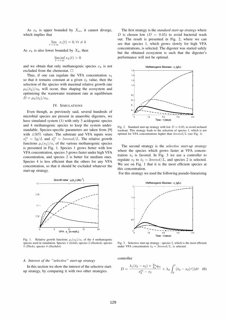
As xk is upper bounded by Xm, it cannot diverge,
which implies that
limt→+∞
xi(t) = 0,∀i 6= k
As xk is also lower bounded by X0, then
lim inft→+∞
xk(t) > 0
and we obtain that only methanogenic species xk is not
excluded from the chemostat. �
Thus, if one can regulate the VFA concentration s2
so that it remains constant at a given s2 value, then the
selection of the species with maximal relative growth rate
µk(s2)/αk will occur, thus shaping the ecosystem and
optimizing the wastewater treatment rate at equilibrium
D = µk(s2)/αk.
IV. SIMULATIONS
Even though, as previously said, several hundreds of
microbial species are present in anaerobic digesters, we
have simulated system (1) with only 3 acidogenic species
and 4 methanogenic species to keep the system under-
standable. Species-specific parameters are taken from [9]
with ±50% values. The substrate and VFA inputs were
sin1 = 5g/L and sin
2 = 5mmol/L. The relative growth
functions µi(s2)/αi of the various methanogenic species
is presented in Fig. 1. Species 1 grows better with low
VFA concentration, species 3 grows faster under high VFA
concentration, and species 2 is better for medium ones.
Species 4 is less efficient than the others for any VFA
concentration, so that it should be excluded whatever the
start-up strategy.
Fig. 1. Relative growth functions µi(s2)/αi of the 4 methanogenicspecies used in simulation. Species 1 (Solid), species 2 (Dashed), species3 (Thick), species 4 (Dashdot)
A. Interest of the ”selective” start-up strategy
In this section we show the interest of the selective start-
up strategy, by comparing it with two other strategies.
The first strategy is the standard start-up strategy where
D is chosen low (D = 0.05) to avoid bacterial wash
out. The result is presented in Fig. 2, where we can
see that species 1, which grows slowly for high VFA
concentrations, is selected. The digester was started safely
but the obtained ecosystem is such that the digester’s
performance will not be optimal.
Fig. 2. Standard start-up strategy with low D = 0.05, to avoid archaealwashout. This strategy leads to the selection of species 1, which is notoptimal for VFA concentrations higher than 2mmol/L (see Fig. 1)
The second strategy is the selective start-up strategy
where the species which grows faster at VFA concen-
tration s2 is favored. In Fig. 3 we use a controller to
regulate s2 to s2 = 3mmol/L, and species 2 is selected.
We see on Fig. 1 that it is the most efficient species at
this concentration.
For this strategy we used the following pseudo-linearizing
Fig. 3. Selective start-up strategy : species 2, which is the most efficientunder VFA concentration s2 = 3mmol/L, is selected.
controller
D =λ1(s2 − s2) + k3
k4
qm
sin2 − s2
+ λ2
∫ t
0
(s2 − s2(τ))dτ (6)
129
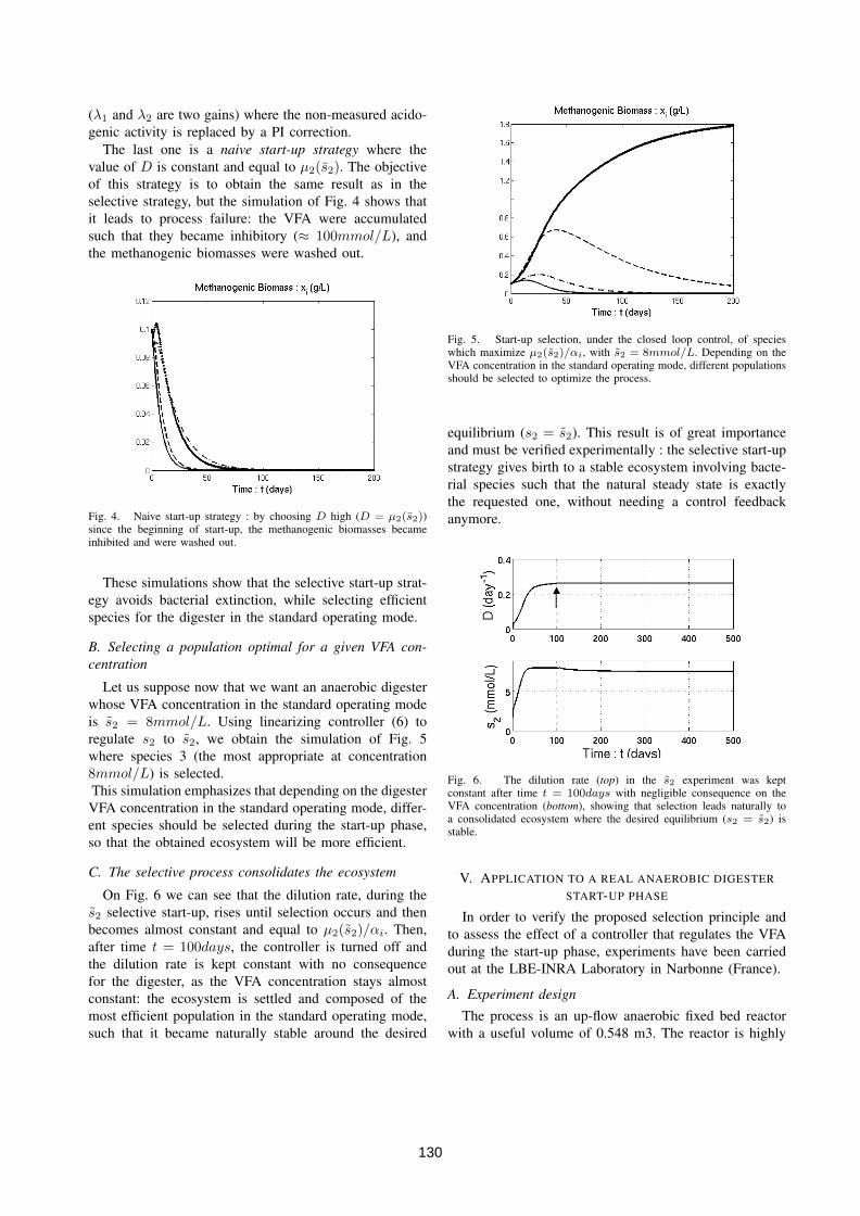
(λ1 and λ2 are two gains) where the non-measured acido-
genic activity is replaced by a PI correction.
The last one is a naive start-up strategy where the
value of D is constant and equal to µ2(s2). The objective
of this strategy is to obtain the same result as in the
selective strategy, but the simulation of Fig. 4 shows that
it leads to process failure: the VFA were accumulated
such that they became inhibitory (≈ 100mmol/L), and
the methanogenic biomasses were washed out.
Fig. 4. Naive start-up strategy : by choosing D high (D = µ2(s2))since the beginning of start-up, the methanogenic biomasses becameinhibited and were washed out.
These simulations show that the selective start-up strat-
egy avoids bacterial extinction, while selecting efficient
species for the digester in the standard operating mode.
B. Selecting a population optimal for a given VFA con-
centration
Let us suppose now that we want an anaerobic digester
whose VFA concentration in the standard operating mode
is s2 = 8mmol/L. Using linearizing controller (6) to
regulate s2 to s2, we obtain the simulation of Fig. 5
where species 3 (the most appropriate at concentration
8mmol/L) is selected.
This simulation emphasizes that depending on the digester
VFA concentration in the standard operating mode, differ-
ent species should be selected during the start-up phase,
so that the obtained ecosystem will be more efficient.
C. The selective process consolidates the ecosystem
On Fig. 6 we can see that the dilution rate, during the
s2 selective start-up, rises until selection occurs and then
becomes almost constant and equal to µ2(s2)/αi. Then,
after time t = 100days, the controller is turned off and
the dilution rate is kept constant with no consequence
for the digester, as the VFA concentration stays almost
constant: the ecosystem is settled and composed of the
most efficient population in the standard operating mode,
such that it became naturally stable around the desired
Fig. 5. Start-up selection, under the closed loop control, of specieswhich maximize µ2(s2)/αi, with s2 = 8mmol/L. Depending on theVFA concentration in the standard operating mode, different populationsshould be selected to optimize the process.
equilibrium (s2 = s2). This result is of great importance
and must be verified experimentally : the selective start-up
strategy gives birth to a stable ecosystem involving bacte-
rial species such that the natural steady state is exactly
the requested one, without needing a control feedback
anymore.
Fig. 6. The dilution rate (top) in the s2 experiment was keptconstant after time t = 100days with negligible consequence on theVFA concentration (bottom), showing that selection leads naturally toa consolidated ecosystem where the desired equilibrium (s2 = s2) isstable.
V. APPLICATION TO A REAL ANAEROBIC DIGESTER
START-UP PHASE
In order to verify the proposed selection principle and
to assess the effect of a controller that regulates the VFA
during the start-up phase, experiments have been carried
out at the LBE-INRA Laboratory in Narbonne (France).
A. Experiment design
The process is an up-flow anaerobic fixed bed reactor
with a useful volume of 0.548 m3. The reactor is highly
130

instrumented and many variables were measured during
the experiments [9]. More details about the process and
evaluation of its on-line instrumentation are available in
[14].
B. Experimental results and discussion
Control (6) was applied, with command s2 = 4 g/L,
and control parameters k3 = 116.5 mmol/g, k4 = 453mmol/g, λ1 = 12 day−1 and λ2 = 0.05 mmol−1 day−1 .
The experimental results are presented in Fig. (7).
Time (days)
Time (days)
VF
A (
g/L)
Qin
(L/h
)
Fig. 7. Start-up experiment where s2 is regulated at s2 = 4g/L. Theinfluent flow rate (Qin = D/V ) and the VFA concentration are plotted.
We can see on this figure that our control objective
was attained : the VFA concentration was well driven
towards s2 despite many disturbances related to failures
and disturbances in the process. It is worth noting that
the more the ecosystem is selected, the more efficient the
regulation. At the end, when the interesting species have
probably been selected in the digester, the regulation is
more and more efficient.
Finally, the proposed strategy enabled us to reach a high
dilution rate D = 0.78 while avoiding start-up failure.
VI. CONCLUSIONS
We proposed a start-up strategy for an anaerobic di-
gester, whose aim is to influence the structure of the
ecosystem, so that the obtained ecosystem in the end of
start-up will be optimal for a given VFA concentration.
For implementing such a selective process, we drive the
competition by regulating the VFA concentration at a fixed
value. We showed how the obtained ecosystem should also
be consolidated because of the selection that occurs during
the start-up phase.
According to model (1), a control law was proposed and
a mathematical demonstration was given for predicting the
competition outcome. Simulations were used to verify and
explain the utility of the method, and a real experiment
was presented where the start-up strategy was tested.
We emphasize that the aim of this strategy is not
to minimize the start-up duration, but rather to build
an efficient ecosystem. This kind of start-up strategy,
where the objective is to act on the bacterial community’s
structure for optimizing a particular process, was never
(to our knowledge) proposed before for anaerobic diges-
tion. Further investigations in this direction are presently
performed.
VII. ACKNOWLEDGMENTS
This work was carried out with support provided by the
CODA ARC project funded by the INRIA.
REFERENCES
[1] C. Delbes, R. Moletta, and J.-J. Godon, “Bacterial and archaeal 16srdna and 16s rrna dynamics during an acetate crisis in an anaerobicdigestor ecosystem,” FEMS Microbiology Ecology, vol. 35, pp. 19–26, 2001.
[2] J. Hess and O. Bernard, “Design and study of a risk managementcriterion for an unstable anaerobic wastewater treatment process,”J. Process. Contr., vol. 18, pp. 71–79, 2008.
[3] K.-Y. how.and Y. Wang, S.-F. Foong, and J.-H.Tay, “Acceleratedstart-up and enhanced granulation in upflow anaerobic sludgeblanket reactors,” Water Research, vol. 28, pp. 2293–2304, 2004.
[4] S. Michaud, N. Bernet, P. Buffiere, M. Roustan, and R. Moletta,“Methane yield as a monitoring parameter for the strat-up ofanaerobic fixed film reactors,” Water Research, vol. 36, pp. 1385–1391, 2002.
[5] J. S. I. Ramirez, E.I.P. Volcke, “Modeling and monitoring of micro-bial diversity in ecosystems - application to biological wastewatertreatment processes,” in Proceedings of the IFAC conference.Seoul, Korea, 2008.
[6] H. L. Smith and P. Waltman, The theory of the chemostat: dynamics
of microbial competition. Cambridge University Press, 1995.[7] S. R. Hansen and S. P. Hubbell, “Single-nutrient microbial com-
petition,” Science, vol. 207, no. 28, pp. 1491–1493, 1980.[8] P. Masci, F. Grognard, and O. Bernard., “Continuous selection of
the fastest growing species in the chemostat,” in Proceedings of
the IFAC conference. Seoul, Korea, 2008.[9] O. Bernard, Z. Hadj-Sadok, D. Dochain, A. Genovesi, and
J.-P. Steyer, “Dynamical model development and parameteridentification for an anaerobic wastewater treatment process,”Biotech.Bioeng., vol. 75, pp. 424–438, 2001.
[10] G. Bastin and D. Dochain, On-line estimation and adaptive control
of bioreactors. Amsterdam: Elsevier, 1990.[11] G. Wolkowicz and L. Zhiqi, “Global show, k.-y.; wang, y.; foong,
s.-f.; tay, j.-h. accelerated start-up and enhanced granulation inupflow anaerobic sludge blanket reactors. water research 2004, 38,2293–2304.dynamics of a mathematical model of competition inthe chemostat: General response functions and differential deathrates,” SIAM Journal of Applied Mathematics, vol. 52, pp. 222–233, 1992.
[12] O. Bernard, Z. Hadj-Sadok, M. Pengov, and D. Dochain, “Mod-elling, monitoring and control of anaerobic digestion processes,”Journal A., vol. 41, pp. 82–88, 2000.
[13] L. Mailleret, O. Bernard, and J.-P. Steyer, “Robust nonlinear adap-tive control for bioreactors with unknown kinetics,” Automatica,vol. 40:8, pp. 365–383, 2004.
[14] J. P. Steyer, J. C. Bouvier, T. Conte, P. Gras, and P. Sousbie, “Evalu-ation of a four year experience with a fully instrumented anaerobicdigestion process,” Water Science and Technology, vol. 45, pp. 495–502, 2002.
131

132

Chapter 5
Conclusion
Microbial ecosystems play key roles in our biosphere: they highly contribute toharvest light energy from the sun and to recycle nutrients. They should thereforebe better understood, both for a better apprehension of natural ecosystems butalso for developing cleaner biotechnologies. The implications of the ecosystemsstudied in this thesis are multiple:
• microalgal and anaerobic ecosystems both play an important role in globalwarming since they respectively consume CO2 and produce CH4. Thus,they should be better understood and models must quantify the associatedcarbon and energy fluxes.
• some microalgae, like spirulina, can be eaten and are great potentialsources of proteins, vitamins and minerals [42];
• some microalgae produce pharmaceutics and neutraceutics [38];
• some others produce oil which can be used as a biofuel, and high produc-tivities seem possible [8];
• anaerobic bacteria can clean wastewater, and degrade low biodegradablesubstrates,
• methanogenic bacteria produce methane which is also a renewable biofuel.
Our first step to better apprehend these ecosystems was to develop modelsfor microalgae populations in photobioreactors (chapter 2.1). The model neededto include enough ingredients to reproduce the main process behavior, but hadto be kept simple enough to be validable, identifiable, and to be mathematicallytractable. Our model represents nutrients absorption and storage. This is a keyissue for biofuel production since nitrogen influences lipids synthesis (see ourlipid synthesis model in [33]). It also represents light attenuation and respira-tion which are crucial when biomass concentration is high, which is often thecase in real bioprocesses. The last ingredients are photoinhibition (high lightintensities inhibit growth) and photoacclimation (Chl/C ratio variations de-pending on the received light) which is important when light or biomass vary inthe photobioreactor. While representing all these phenomena, the model staysrelatively simple, based on only four dynamical equations representing nitrogenin the medium, biomass, internal nitrogen quota, and chlorophyll evolutions.
133

A parameter calibration procedure is proposed and used to validate themodel on a dataset. Analytical results demonstrate that high density cultures,when subject to photoinhibition under strong light, show no apparent photoin-hibition, as only the little proportion of microalgae near the reactor’s incidentsurface are photoinhibited. This explains why photoinhibition is not always ob-served in high density cultures. However, photoinhibition induces a hidden lossthat must be considered and, if possible, avoided.
With a variant of this model, where photoadaptation was assumed to be atequilibrium, we proceeded to an optimization of biomass surface productivity atequilibrium (chapter 3.1). We showed that a key parameter is surface biomassX: the photobioreactor acts like a solar panel where surface biomass enablesto gather light energy, but causes energy losses by respiration. An optimalsurface biomass is derived, as well as an optimal nitrogen/carbon quota. Theresult is counter-intuitive, as it states that depending on the microalgal speciesparameters, it might be optimal to grow microalgae in nutrient limited condi-tions. Indeed, for a fixed high biomass, higher nitrogen/carbon ratio correspondto higher chlorophyll concentration and thus strong light attenuation, causinglower growth rate.
Productivity is the result of many biological and physical interacting phe-nomena, the most important of which are represented in the DPM model. Thatis why the productivity is a complex combination of several model parameters.This results enables to compare microalgal species productivity, which can becomputed directly from their parameters.
As microalgae must be grown into natural light for biofuel production (forhigh value products they are sometimes grown under artificial light), they en-counter day-night light variations. In the case of nutrient profusion (chapter3.2), we show that several optimal control scenarii must be applied for optimiz-ing volumetric productivity, depending on the microalgal species parameters:bang-bang, bang-singular-bang control, or constant maximal dilution if the mi-croalgal growth rate is very high.
Finally we gave some key results for competition study and control. Theanalysis of mixed competition between several Monod, Droop and Contois species(section 4.1) introduces a new paradigm for competition, where both competi-tive exclusion or coexistence can happen, depending on both species parametersand controls. Thus in this paradigm, neither competitive exclusion nor coexis-tence are the rule; one or the other can happen, depending on the species andenvironmental conditions. More precisely, in some cases the most competitiveMonod or Droop species wins the competition alone. In other cases one orseveral Contois species are able to coexist with or without the best Monod orDroop competitor. The pessimization principle of Adaptive dynamics, basedon the competitive exclusion principle, is contradicted by this result: instead ofleaving the environment with the worst (lowest) possible substrate concentra-tion, we see that some Contois-species could live in worse environments, but ifthere is more substrate than the minimal concentration they need, then someother species can coexist. This is due to the fact that higher input substrateconcentration induces higher equilibrium biomass, and thus higher equilibriumsubstrate concentration needed to have growth rate β(s, x) equal to the dilutionrate D.
134

Then (section 4.2) we demonstrate rigorously that in the periodic turbido-stat, the species with highest mean growth rate wins the competition. Thisgives us the possibility to control competition in order to select species withdiverse characteristics. In particular, we prove that in the classical turbidostat(nutrient replete conditions), the species with highest maximum growth rateis selected. In the pulsed turbidostat we show that the selected species maxi-mizes a criterion which is a trade-off between high maximum growth rate (µm),and high potential increase of its internal substrate storage (Qm/Q0). Theseapplications had already been validated in three previous distinct experimentsconcerning different types of microorganisms (zooplankton [4], yeast [18], andmicroalgae [20]).
We extended this methodology to the more complex anaerobic ecosystemduring its start-up phase (chapter 4.3), in order to favour an efficient biofilmwhich would maximize the wastewater treatment rate. This should also increasethe methane production rate.
This work is a whole that can be continued in each of these three directions:modelling, optimization, competition study and control.
The DPM and lipid synthesis models must be confronted with experiments,in order to be validated or improved. In particular, the simulated result thatphotoinhibition is not perceptible but present in high density cultures shouldbe validated by a devoted experiment.
The optimization result, that for some microalgal population parameters,nitrogen limited cultures could have higher biomass productivities than nitro-gen replete ones, should also be explored experimentally. Many optimizationresearch remains to be done under day-night cycles with non-nitrogen repleteculture, as well as for lipids production maximization. Some factors, like tem-perature or pH, could also be added to the DPM model in order to explore theireffect on productivity. Much work and experiments remain to be done in thisdirection.
For competition theory, it would be interesting to validate the mixed com-petition result, by doing an experiment with Monod/Droop species and Contoisspecies and verifying if the diverse competitive exclusion and coexistence out-comes can be produced and precisely controlled.
Then, the proposed selection procedures in microalgal and methanogenicbacteria ecosystems should be tested both on the short term (validation ofthe predicted outcome of competition), and on the long run: to see if species /biofilms with improved characteristics can be selected with these methods. Suchresults would gives some hope for alternative techniques to GMO organisms, inorder to improve ecosystem’s efficiency. This method could also be used to iden-tify species which grow in hostile conditions, to amplify and verify the presenceof a species in a medium, or to determine conditions which permit a species tobe resistant to invaders. The selection criterion, which is the maximum meangrowth rate in chosen environmental conditions, seems very promising and cantake different forms depending on the imposed environmental conditions: thiswork could be extended by using other controls such as an inhibitor’s concen-tration, or light in the case of microalgae. This would lead to new selectioncriteria.
135
We stress again that many factors should be taken into account for choosinga microalgal species that maximizes surface productivity: microalgal resistanceto temperature shifts or to predation, and the various effects of the local en-vironment affecting growth of a specific microalgal species. For this purpose,models including additional factors, like temperature or pH, must be developedand explored analytically. The steps of modelling, optimization and competi-tion prediction and control must then be revisited with these new factors. Wehope to have participated in creating solid bases for the undertaking of such along term task.
Both the competition prediction and controls works presented here show thebeauty of mathematics. We have highlighted the ability of mathematical mod-elling for giving ecological insight in a very general sense: the same equationsand methodologies enable to successfully describe different ecosystems, frommicroalgae to bacteria and yeast.
136
Conclusion
Les écosystèmes microbiens jouent un rôle clé dans notre biosphère: ils con-tribuent significativement à intégrer l’énergie lumineuse du soleil au cycle de lavie, et à recycler les éléments nutritifs. Ils devraient donc être mieux compris,à la fois pour une meilleure appréhension des écosystèmes naturels, mais égale-ment pour le développement de biotechnologies propres. Les implications desécosystèmes étudiés dans cette thèse sont multiples:
• les écosystèmes de microalgues et de digestion anaérobie jouent un rôleimportant dans le réchauffement climatique, car les premiers consommentdu CO2 et les seconds produisent du CH4. Ainsi, les modèles doiventquantifier les flux de carbone et d’énergie;
• certaines microalgues, comme la spiruline, peuvent être consommées etsont potentiellement de grandes sources de protéines, vitamines et miné-raux [42];
• certaines microalgues produisent des composés chimiques utilisés dans desproduits pharmaceutiques et nutraceutique [38];
• d’autres produisent de l’huile qui peut être utilisée comme biocarburant,et des productivités élevées semblent possibles [8];
• les bactéries anaérobies peuvent nettoyer les eaux usées, et dégrader dessubstrats faiblement biodégradables,
• les bactéries méthanogènes produisent du méthane qui est un biocarburantrenouvelable.
Notre premier pas pour mieux appréhender ces écosystèmes a été de dévelop-per des modèles de population de microalgues en photobioréacteur (chapitre2.1), le modèle "DPM" (Droop Photobioreactor Model). Le modèle devait in-clure les ingrédients clés permettant de reproduire les comportements principauxdu procédé, mais devait aussi être assez simple pour être validable, identifiable,et mathématiquement analysable. Notre modèle représente l’absorption et lestockage des nutriments. Il s’agit d’une question clé pour la production de bio-carburants, puisque la synthèse de lipides est influencée par la disponibilité enazote dans le milieu (voir la construction du modèle de synthèse des lipides auchapitre 2.2). Il représente également l’atténuation de la lumière et l’influencede la respiration qui sont essentiels lorsque la concentration de la biomasseest élevée, ce qui est souvent le cas dans les bioprocédés réels. Les derniersingrédients sont la photoinhibition (les fortes intensités lumineuses inhibent la
137

croissance) et la photoacclimation (variations du rapport Chl / C en fonction dela lumière reçue), qui sont importants quand la lumière ou la biomasse varientdans le photobioréacteur. Tout en représentant tous ces phénomènes, le mod-èle reste relativement simple, basé sur seulement quatre équations dynamiquesreprésentant l’évolution de l’azote dans le milieu, de la biomasse, du quotad’azote interne, et de la chlorophylle.
Une procédure de calibration des paramètres est proposée et utilisée pourvalider le modèle sur un ensemble de données. Les résultats des analyses dé-montrent que les cultures à haute densité, lorsqu’elles sont soumises à la pho-toinhibition sous une forte lumière, ne montrent pas de photoinhibition appar-ente, puisque seule la petite proportion de microalgues proches de la surfaced’incidence du réacteur sont photoinhibées. Cela explique pourquoi la photoin-hibition n’est pas toujours observée dans les cultures à haute densité. Toutefois,la photoinhibition induit une perte cachée qui doit être examinée et, si possible,évitée.
À partir de données expérimentales obtenues au LOV, nous avons ensuiteconstruit un modèle qui reproduit fidèlement les évolutions des taux de lipideset de sucres (chapitre 2.2).
Avec une variante de notre modèle DPM, où la photoadaptation était àl’équilibre, nous avons procédé à une optimisation de la productivité surfaciquede la biomasse à l’équilibre (chapitre 3.1). Nous avons montré qu’un paramètreclé est la biomasse surfacique X : le photobioréacteur agit comme un panneausolaire où la biomasse permet d’exploiter l’énergie lumineuse mais provoque despertes d’énergie par respiration. Une biomasse surfacique et un quota interneazote/carbone optimaux sont calculés. Le résultat est contre-intuitif, car ilindique que, selon les paramètres de l’espèce de microalgues considérée, il pour-rait être optimal de faire pousser les microalgues dans des conditions limitées enazote. En effet, pour une biomasse fixée élevée, un fort rapport azote/carbonecorrespond à une forte concentration en chlorophylle et donc une plus forteatténuation de la lumière, provoquant un taux de croissance plus faible.
La productivité est le résultat de nombreux phénomènes biologiques et phy-siques qui interagissent, et dont les plus importants sont représentés dans lemodèle DPM. C’est pourquoi la productivité est une combinaison complexe deplusieurs paramètres du modèle. On peut donc comparer la productivité dedifférentes espèces de microalgues, en la calculant directement à partir de leursparamètres.
Comme les microalgues doivent être cultivées sous lumière naturelle pour laproduction de biocarburants (les microalgues qui synthétisent des composants àhaute valeur ajoutée sont parfois cultivées sous lumière artificielle), elles subis-sent les variations jour-nuit de la lumière. Dans le cas d’une profusion en élé-ments nutritifs (chapitre 3.2), nous montrons que plusieurs scénarios de con-trôle optimal peuvent être appliqué pour optimiser la productivité volumétrique,selon les paramètres de l’espèce de microalgues considérée : bang - bang, bang- arc singulier - bang, ou taux de dilution maximal si le taux de croissance desmicroalgues est très élevé.
Enfin, nous avons donné quelques résultats clés pour l’étude et le contrôlede la compétition. L’analyse de la compétition mixte entre plusieurs espècesreprésentées par les modèles de Monod, Droop et Contois (section 4.1) introduit
138

un nouveau paradigme de la compétition, où exclusion compétitive et coexis-tence peuvent tous deux survenir, en fonction des paramètres des espèces etdes contrôles utilisés. Ainsi, dans ce paradigme, ni l’exclusion compétitive ni lacoexistence ne sont la règle; l’un ou l’autre peut se produire, selon les espècesen compétition et les conditions environnementales. Plus précisément, danscertains cas, la plus compétitive des espèces de Monod et de Droop remporteseule la compétition. Dans d’autres cas une ou plusieurs espèces de Contoissont capables de coexister avec ou sans le meilleur des concurrents de Monodet Droop. Le "Pessimization principle" de la Dynamique Adaptative, basé surle principe de l’exclusion compétitive, est contredit par ce résultat : au lieu delaisser l’environnement avec la pire (la plus basse) concentration du substratpossible, nous voyons que certaines espèces de Contois pourraient vivre dansde pires environnements, mais s’il y a plus de substrat que la concentrationminimale dont ils ont besoin, alors d’autres espèces peuvent coexister. Celaest dû au fait qu’une concentration plus élevée de substrat en entrée provoqueune biomasse à l’équilibre plus élevée, et donc une concentration plus élevée desubstrat à l’équilibre pour avoir un taux de croissance β(s, x) égal au taux dedilution D.
Ensuite (section 4.2) nous avons démontré de façon rigoureuse que dans unturbidostat périodique, l’espèce avec le taux de croissance moyen le plus élevégagne la compétition. Cela nous donne la possibilité de contrôler la compétitionafin de sélectionner des espèces présentant diverses caractéristiques. En partic-ulier, nous avons montré que dans le turbidostat classique (profusion d’élémentsnutritifs), l’espèce avec le taux de croissance maximal le plus élevé est sélection-née. Dans le turbidostat pulsé nous avons montré que l’espèce sélectionnéemaximise un critère qui est un compromis entre un taux de croissance maxi-mal élevé (µm), et une forte augmentation potentielle de son stock interne denutriment (Qm/Q0). Ces applications avaient déjà été validées dans trois ex-périences distinctes précédentes portant sur différents types de micro-organismes(zooplancton [4], levure [18], et les microalgues [20]).
Nous avons étendu cette méthodologie à l’écosystème plus complexe de ladigestion anaérobie au cours de sa phase de démarrage (chapitre 4.3), afin defavoriser un biofilm efficace qui permettrait de maximiser la vitesse de traite-ment des eaux usées. Cela devrait également augmenter le taux de productionde méthane.
Ce travail est un tout qui peut être poursuivi dans chacune de ces troisdirections : modélisation, optimisation, étude et contrôle de la compétition.
Les modèles DPM et de synthèse de lipides doivent être confrontés à d’avantaged’expériences, afin d’être validés ou améliorés. En particulier, le résultat simuléque la photoinhibition n’est pas perceptible, mais présente dans les cultures àhaute densité, devrait être validé par une expérience dédiée.
Le résultat d’optimisation, stipulant que pour certains paramètres de la pop-ulation de microalgues, des cultures limitées en azote pourraient avoir des pro-ductivités de biomasse supérieures à celles qui ne sont pas limitées, devrait égale-ment être étudié expérimentalement. Beaucoup reste à faire pour l’optimisationen cycles jour-nuit avec des cultures non limitées en azote, ainsi que pour la max-imisation de la production de lipides. Certains facteurs, comme la températureou le pH, peuvent également être ajoutés au modèle DPM afin d’explorer leurseffets sur la productivité. Beaucoup de travail et d’expériences restent à faire
139
dans cette direction.Pour la théorie de la compétition, il serait intéressant de valider le résultat
de la compétition mixte, en faisant une expérience avec des espèces représentéespar les modèles de Monod, de Droop, et de Contois, et de vérifier si exclusioncompétitive et coexistence peuvent tous deux être obtenus et contrôlés avecprécision.
Ensuite, les procédures de sélection proposées pour les écosystèmes de mi-croalgues, et de bactéries méthanogènes, devraient être testées à la fois sur lecourt terme (validation de la prédiction du résultat de la compétition), et sur lelong terme : pour voir si des populations aux caractéristiques améliorées peu-vent être sélectionnés avec ces méthodes. De tels résultats donnent un espoirpour améliorer l’efficacité de ces écosystèmes sans avoir recours aux OGM. Cetteméthode pourrait également être utilisée pour identifier les espèces qui poussentdans des conditions hostiles, pour amplifier et vérifier la présence d’une espècedans un milieu, ou pour déterminer les conditions qui permettent à une espècede résister aux envahisseurs. Le critère de sélection, qui est le taux de crois-sance moyen maximal dans des conditions environnementales données, sembletrès prometteur et peut prendre différentes formes selon les conditions imposéesà l’environnement : ce travail pourrait être étendu à l’aide d’autres contrôles telsque la concentration d’un inhibiteur, ou la lumière dans le cas de microalgues.Cela conduirait à de nouveaux critères de sélection.
Nous soulignons à nouveau que de nombreux facteurs doivent être pris encompte pour le choix d’espèces de microalgues qui maximisent la productivitésurfacique : la résistance des microalgues aux variations de température ou à laprédation, et les divers effets de l’environnement local qui affectent la croissanced’une espèce particulière de microalgues. Dans ce but, des modèles incluantd’autres facteurs, comme la température ou le pH, doivent être développés etétudiés analytiquement. Les étapes de modélisation, d’optimisation et de prédic-tion et contrôle de la compétition devront alors être revisitées avec ces nouveauxfacteurs. Nous espérons avoir participé à la création de bases solides pour laréalisation de cette longue tâche.
Les résultats sur la prédiction de l’issue de la compétition et son contrôlemontrent la beauté des mathématiques. Nous avons mis en évidence la capacitéde la modélisation mathématique à développer la compréhension écologique dansun sens très général : les mêmes équations et méthodes permettent de décrireavec succès des écosystèmes différents, des microalgues jusqu’aux bactéries etaux levures.
140

Bibliography
[1] R. Armstrong & R. McGehee – “Competitive exclusion”, AmericanNaturalist 115 (1980), p. 151.
[2] J. E. Bailey & D. F. Ollis – Biochemical engineering fundamentals,McGraw-Hill, 1986.
[3] J. Benemann – “Co2 mitigation with microalgae systems”, Energy Con-version and Management (1997), p. 475–479.
[4] W. Bennett & M. Boraas – “Isolation of a fast-growing strain of therotifer brachionus calyciflorus pallas using turbidostat culture”, Aquacul-ture(Amsterdam) 73 (1988), no. 1-4, p. 27–36.
[5] B. C. Benson & K. A. Rusch – “Investigation of the light dynamicsand their impact on algal growth rate in a hydraulically integrated se-rial turbidostat algal reactor (histar)”, Aquacultural engineering 35 (2006),p. 122–134.
[6] O. Bernard, Z. Hadj-Sadok, D. Dochain, A. Genovesi & J.-P.Steyer – “Dynamical model development and parameter identificationfor an anaerobic wastewater treatment process”, Biotech.Bioeng. (2001),no. 75, p. 424–438.
[7] J.-P. Cadoret & O. Bernard – “La production de biocarburants li-pidique avec des microalgues: promesses et défis”, Journal de la socété debiologie 202 (2008), p. 201–211.
[8] Y. Chisti – “Biodiesel from microalgae”, Biotechnology Advances 25
(2007), p. 294–306.
[9] D. Contois – “Kinetics of bacterial growth: relationship between pop-ulation density and specific growth rate of continuous cultures.”, J GenMicrobiol. (1959), p. 40–50.
[10] C. Darwin – On the origin of species by means of natural selection, or thepreservation of favoured races in the struggle for life, John Murray, 1859.
[11] C. Delbès, R. Moletta & J.-J. Godon – “Bacterial and archaeal 16srdna and 16s rrna dynamics during an acetate crisis in an anaerobic digestorecosystem”, FEMS Microbiology Ecology 35 (2001), p. 19–26.
[12] O. Diekmann – “A beginner’s guide to adaptive dynamics”, Banach Cen-ter Publ. (2003), p. 47–86.
140
141
[13] M. Droop – “Vitamin b12 and marine ecology”, J. Mar. Biol Assoc. U.K.48 (1968), p. 689–733.
[14] D. Dykhuizen & D. Hartl – “Selection in chemostats.”, Microbiologicalreviews. Baltimore 47 (1983), no. 2, p. 150–168.
[15] B. Ewing, S. Goldfinger, A. Oursler, A. Reed, D. Moore &M.Wackernagel. – The ecological footprint atlas 2009., 2009.
[16] P. G. Falkowski & J. A. Raven – Aquatic photosynthesis, BlackwellScience, 2007.
[17] G. Gause – The struggle for existence, Williams and Wilkins, Baltimore,1934.
[18] P. Groeneveld, A. Stouthamer & H. Westerhoff – “Super life -how and why ’cell selection’ leads to the fastest-growing eukaryote”, FEBSJournal 276 (2008), p. 254–270.
[19] F. Grognard, F. Mazenc & A. Rapaport – “Polytopic lyapunov func-tions for persistence analysis of competing species”, Discrete and Continu-ous Dynamical Systems-Series B 8 (2007), no. 1, p. 73–93.
[20] J. Grover – “Dynamics of competition among microalgae in variable envi-ronments: experiment tests of alternative models”, Oikos 62 (1991), p. 231–243.
[21] B. Haegeman, C. Lobry & J. Harmand – “Modeling bacteria floccu-lation as density-dependent growth”, AICHE JOURNAL 53 (2007), no. 2,p. 535–539 (English).
[22] S. Hansen & S. Hubell – “Single-nutrient microbial competition: qual-itative agreement between experimental and theoretically forecast out-comes”, Science 207 (1980), no. 4438, p. 1491–1493.
[23] G. Hardin – “The competitive exclusion principle”, Science 131 (1960),no. 3409, p. 1292–1297.
[24] G. P. Harris – Phytoplankton ecology, Chapman and hall, 1986.
[25] S. Hsu & T. Hsu – “Competitive exclusion of microbial species for a single-nutrient with internal storage”, SIAM Journal on Applied Mathematics 68
(2008), no. 6, p. 1600–1617.
[26] M. Huntley & D. Redalje – “Co2 mitigation et renewable oil from pho-tosynthetic microbes: A new appraisal”, Mitigation et Adaptation Strate-gies for Global Change 12 (2007), p. 573 – 608.
[27] G. E. Hutchinson – “The paradox of the plankton”, The American Nat-uralist 95 (1961), p. 137.
[28] A. Jacquard – Le compte à rebours a-t-il commencé ?, Stock, 2009.
[29] C. Jessup, S. Forde & B. Bohannan – “Microbial experimental systemsin ecology”, Advances in Ecological Research 37 (2005), p. 273–306.
142

[30] T. Lacour – “Influence du statut azoté et du cycle lumineux diurne sur lemétabolisme lipidique d’isochrysis sp. (haptophyceae).”, Thèse, Universitéde la méditerranée (Aix-Marseille 2), 2010.
[31] C. Lobry & J. Harmand – “A new hypothesis to explain the coexistenceof n species in the presence of a single resource”, Comptes Rendus Biologies329 (2006), no. 1, p. 40–46.
[32] C. Lobry, F. Mazenc & A. Rapaport – “Persistence in ecological mod-els of competition for a single resource”, Comptes Rendus Mathematique340 (2005), no. 3, p. 199–204.
[33] F. Mairet, O. Bernard, P. Masci, T. Lacour & A. Sciandra –“Modelling lipid prduction in microalgae”, in Proceedings of the CAB con-ference, 2010.
[34] M. G. Malea, F. Ancíen, M. C. J.M. Fernández & E. Molina –“Continuous production of green cells of haematococcus pluvialis: Model-ing of the irradiance effect”, Enzyme and microbial technology 38 (2006),p. 981–989.
[35] F. Mazenc & Z.-P. Jiang – “Persistence and time-varying nonlinearcontrollers for a chemostat with many species”, Dynamics of Continuous,Discrete and Impulsive Systems (2010), p. to appear.
[36] J. Monod – “Recherches sur la croissance des cultures bacteriennes”,Paris: Herrmann et Cie (1942).
[37] Y. Percival Zhang, M. Himmel & J. Mielenz – “Outlook for cellulaseimprovement: Screening and selection strategies”, Biotechnology Advances24 (2006), no. 5, p. 452–481.
[38] O. Pulz – “Photobioreactors: production systems for phototrophic mi-croorganisms”, Applied Microbiology et Biotechnology 57 (2001), p. 287–293.
[39] O. N. Ross & R. J. Geider – “New cell-based model of photosynthesisand photo-acclimatation: accummulation and mobilisation of energy re-serves in phytoplankton”, Marine ecology progress series 383 (2009), p. 53–71.
[40] F. C. Rubio, F. G. Camacho, J. F. Sevilla, Y. Chisti & E. M.Grima – “A mechanistic model of photosynthesis in microalgae”, Biotech-nology and Bioengineering 81 (2003), no. 4, p. 459–473.
[41] H. Smith & P. Waltman – The theory of the chemostat. dynamics ofmicrobial competition, Cambridge Studies in Mathematical Biology. Cam-bridge University Press, 1995.
[42] P. Spolaore, C. Joannis-Cassan, E. Duran & A. Isambert – “Com-mercial applications of microalgae”, Journal of Bioscience and Bioengi-neering 101 (2006), no. 2, p. 87 – 96.
[43] D. Tilman – “Resource competition between plankton algae: An experi-mental and theoretical approach.”, Ecology 58 (1977), no. 22, p. 338–348.
143

[44] D. Tilman & R. Sterner – “Invasions of equilibria: tests of resourcecompetition using two species of algae”, Oecologia 61 (1984), no. 2, p. 197–200.
[45] M. Wackernagel & W. Rees – “Perceptual and structural barriers toinvesting in natural capital: Economics from an ecological footprint per-spective”, Ecol. Econom. 20 (1997), no. 1, p. 3–24.
[46] J. B. Wilson – “Mechanisms of species coexistence: twelve explanationsfor the hutchinson’s ’paradox of the phytoplankton’: evidence from newzealand plant communities”, New Zealand journal of Ecology 17–42 (1990),p. 137.
[47] O. Zelder & B. Hauer – “Environmentally directed mutations and theirimpact on industrial biotransformation and fermentation processes”, Cur-rent Opinion in Microbiology 3 (2000), p. 248–251.
144

List of publications
Olivier Bernard, Pierre Masci, Francis Mairet and Antoine Sciandra, A photo-bioreactor model in nitrogen limited conditions, submitted to Biotechnology &Bioengineering
Pierre Masci, Frédéric Grognard, Eric Benoît, Olivier Bernard, Competitionbetween diverse types of microorganisms : exclusion and coexistence, submittedto Mathematical Biosciences and Engineering
Pierre Masci and Olivier Bernard and Frédéric Grognard, Continuous Selec-tion of the Fastest Growing Species in the Chemostat, 2008, Proceedings of theIFAC conference (p. 9707-9712)
Olivier Bernard and Pierre Masci and Antoine Sciandra, A photobioreactormodel in nitrogen limited conditions, 2009, Proceedings of the Mathmod 09 con-ference
P. Masci and O. Bernard and F. Grognard and E. Latrille and J.-B. Sorbaand J.P. Steyer, Driving competition in a complex ecosystem : application toanaerobic digestion, 2009, Proceedings of the ECC conference
F. Mairet, O. Bernard, P. Masci, T. Lacour, A. Sciandra, Modelling lipidproduction in microalgae, 2010, Proceedings of the CAB conference
Pierre Masci, Olivier Bernard, Frédéric Grognard, Microalgal biomass sur-face productivity optimization based on a photobioreactor model, 2010, Proceed-ings of the CAB conference
Frédéric Grognard, Andrei Akhmetzhanov, Pierre Masci and Olivier Bernard,Optimization of a photobioreactor biomass production using natural light, 2010,CDC10 conference
145

Confidential deliverables for
the ANR-06-BIOE-014
Shamash project
Pierre Masci, Olivier Bernard, Frédéric Grognard, Bruno Sialve, Etude théoriquedes conditions de croissance permettant la sélection continue d’espèces max-imisant la production d’huiles, 2008
Pierre Masci, Olivier Bernard, Frédéric Grognard, Development of dynami-cal models to predict lipid production and accumulation in microalgal cultures,2008
Olivier Bernard, Pierre Masci, Frédéric Grognard, Francis Mairet, Premierrapport sur les stratégies théoriques de limitation et de stress maximisant la pro-ductivité lipidique, 2008
Olivier Bernard, Pierre Masci, Frédéric Grognard, Francis Mairet, Secondreport on stress or limitation strategies to maximize oil surface productivity,2009
146

147

148
Résumé
Des biocarburants alternatifs, utilisant des écosystèmes microbiens, sont actuelle-ment étudiés dans le but de limiter la consommation non raisonnée de ressourcesénergétiques et le rejet de gaz à effet de serre, qui modifient le climat. Dans cettethèse, nous avons considéré des bioréacteurs à base de microalgues oléagineuses,et des écosystèmes bactériens anaérobies qui décomposent des déchets et pro-duisent du méthane. Ces travaux avaient pour objectif de mieux comprendre cesprocédés et d’en améliorer les performances. Nous avons tout d’abord modéliséet étudié des cultures de microalgues en photobioréacteurs, dans lesquels les pig-ments algaux induisent une forte atténuation lumineuse. Pour les écosystèmesbactériens, nous avons utilisé un modèle précédemment développé. A l’aide deces modèles et de leur analyse mathématique rigoureuse, nous avons proposédes stratégies pour optimiser leur productivité. Ensuite, l’étude de la sélectionnaturelle entre plusieurs espèces de microorganismes dans ces deux écosystèmesa permis de prédire quelles espèces remportent la compétition. Et finalementnous avons montré comment il est possible, dans chaque écosystème, de con-trôler la compétition pour diriger la sélection naturelle, de façon à avantagerdes espèces ayant des caractéristiques permettant une performance accrue.
Abstract
Some alternative biofuels, produced by microbial ecosystems, are presently stud-ied with the aim of limiting the unreasoned resource consumption of energeticresources, and greenhouse gases emissions which modify the climate. In thisthesis we have considered bioreactors based on oleaginous microalgae, and onanaerobic bacterial ecosystems which degrade wastes and produce methane. Theaims of these works were to better understand these processes and to improvetheir performances. First we have developed and studied models of microalgalcultures in photobioreactors, in which algal pigments cause strong light atten-uation. For anaerobic digestion we have used an existing model. By rigorousmathematical analysis of these models, we propose strategies for optimizingtheir productivity. Then the study of natural selection between several micro-bial species, in these two ecosystems, leads to the prediction of the species whichwins the competition. And finally we showed how it is possible in each ecosys-tem to control competition and drive natural selection, in order to advantagespecies with efficient characteristics, inducing better performances.
149