Control and Adaptive Observer Designs for Managed Pressure...
146
Amirhossein Nikoofard Control and Adaptive Observer Designs for Managed Pressure and Under Balanced Drilling Thesis for the degree of philosophy doctor Trondheim, October 2015 Norwegian University of Science and Technology Faculty of Information Technology, Mathematics and Electrical Engineering Department of Engineering Cybernetics
Transcript of Control and Adaptive Observer Designs for Managed Pressure...

Amirhossein Nikoofard
Control and Adaptive ObserverDesigns for Managed Pressure andUnder Balanced Drilling
Thesis for the degree of philosophy doctorTrondheim, October 2015
Norwegian University of Science and TechnologyFaculty of Information Technology, Mathematics and Electrical EngineeringDepartment of Engineering Cybernetics

NTNUNorwegian University of Science and Technology
Thesis for the degree of philosophy doctor
Faculty of Information Technology, Mathematics and Electrical EngineeringDepartment of Engineering Cybernetics
© 2015 Amirhossein Nikoofard.
ISBN 978-82-326-1392-2 (printed version)ISBN 978-82-326-1393-9 (electronic version)ISSN 1503-8181ITK Report 2016-2-W
Doctoral theses at NTNU, 2016:24
Printed by HP, Canon or Xerox, probably

Dedicated to my parents,and my sisters,
Without whom none of my success would be possible


Summary
Due to increasing the number of depleted formations, reservoirs with lowpressure margins and high cost of field exploration and development, therehas been increasing interest in under-balanced drilling (UBD) and managedpressure drilling (MPD). These types of drillings concepts have contributedto improved oil recovery and reduced drilling problems.
UBD andMPD have several advantages compared to conventional drillingsuch as increasing the ultimate recovery from the reservoir, reducing thenon-productive time (NPT), increasing the rate of penetration (ROP), andextending control over bottom-hole pressure (BHP) for operational scenariossuch as connections and trips and when the rig pumps are off, improvementin safety and well control resulting from more detailed design and planningrequired for accomplishment, decreasing invasive formation damage, and re-ducing drilling problems.
Since the pressure of the well is kept intentionally lower than the pressureof the reservoir in UBD operations, the UBD operations potentially havesome risks and perils. Therefore, it is important to study the control systemand monitoring methodology of UBD operations to improve the safety andefficiency of this method. Underbalanced drilling is not possible for somecases due to existence of high (H2S) in the well or instability in wellbore.
MPD is an alternative overbalanced drilling method which can work on anarrow pressure window and reduce drilling problems. Offshore MPD opera-tion in hostile environment, such as the North Sea, is a challenging problemin drilling, due to heave motion of floating platforms and ships. Withoutproper control, it leads to potential loss of mud, rig blowout and formationkicks. Therefore, it is vital to study the control of offshore MPD operationswith heave motion.
Reservoir properties (i.e. production index, reservoir pore pressure) spec-ify influx of formation fluids during UBD operations. Therefore, reservoircharacterization has a significant effect in the success of UBD. In this work,we develop and compare methods that rely on distributed and low orderlumped models to estimate the states and geological properties of the reser-voir during UBD operation. In this study we also design a controller toattenuate heave disturbance in offshore MPD system.
A nonlinear moving horizon estimation (MHE) based on a nonlinear two-
iii
Summary
phase fluid flow model is designed to estimate the total mass of gas and liquidin the annulus, and geological properties of the reservoir during UBD oper-ation. This observer is evaluated and compared with an Unscented Kalmanfilter for the case of a pipe connection scenario where the main pump isshut off and the rotation of the drill string and the circulation of fluids arestopped. These adaptive observers are compared to each other in terms ofspeed of convergence, sensitivity of noise measurement and accuracy. Theresults show that both algorithms are capable of identifying the produc-tion constants of gas and liquid from the reservoir into the well, while thenonlinear MHE achieves better performance than the Unscented Kalmanfilter.
In addition, a nonlinear Lyapunov-based adaptive observer and an Un-scented Kalman filter based on a low order lumped (LOL) model and an Un-scented Kalman filter based on the distributed drift-flux model are designedto estimate the states and the production constants of gas and liquid fromthe reservoir into the well by using real-time measurements of the choke andthe bottom-hole pressures during UBD operation. These adaptive observersare tested by two scenarios which are simulated with the OLGA simula-tor: a pipe connection scenario and a scenario with a changing productionindex. The OLGA dynamic multiphase flow simulator is a high fidelity sim-ulation tool. The performance of the adaptive observers to detect and trackthe changes in production parameters is studied. Robustness of the adap-tive observers is investigated despite uncertainties in the reservoir and wellparameters of the models. The results show that all adaptive observers arecapable of identifying the production constants of gas and liquid from thereservoir into the well, with some differences in performance. It is also foundthat the LOL model is sufficient for the purpose of reservoir characterizationduring UBD operations.
To estimate unmeasured states, production parameters and slip parame-ters using real time measurements of the bottom-hole pressure and liquid andgas rate at the outlet an Unscented Kalman filter based on simplified drift-flux model is designed. The drift-flux model uses a specific slip law whichallows for transition between single and two phase flows. The performanceis tested against the Extended Kalman Filter by using OLGA simulationsfor two drilling scenarios: a pipe connection scenario and a scenario witha changing production index. The number of cells in the discretization ofthe drift-flux model was found to not have a significant effect on accuracyof estimation. Robustness of the Unscented and Extended Kalman Filtersfor pipe connection scenario is studied in case of uncertainties and errors inthe reservoir and well parameters of the model. The results show that thesemethods are very sensitive to errors in the reservoir pore pressure value.
iv
However, there are robust in case of error in the liquid density value of themodel.
Finally, a constrained model predictive control (MPC) scheme is appliedto MPD operations for controlling of the annular pressure in a well whendrilling from a floating offshore vessel. This controller is evaluated and com-pared with a standard proportional-integral-derivative (PID) control schemeto deal with heave disturbances. The heave disturbances are simulated by astochastic model describing sea waves in the North Sea. The robustness ofthe controller to compensate for heave disturbances despite significant un-certainties in the friction factor and bulk modulus is investigated by MonteCarlo simulations. The results show that the constrained MPC has a goodperformance to regulate the set point and attenuate the effect of the heavedisturbance. Heave motion can be predicted for short time based on forward-looking sensors such as ocean wave radar. It is found that the performanceof MPC can be further improved by prediction of the heave motion about10s ahead.
v

Preface
This thesis is submitted in partial fulfillment of the requirements for the de-gree of Doctor of Philosophy (PhD) at the Norwegian University of Scienceand Technology (NTNU). The research has been conducted at the Depart-ment of Engineering Cybernetics (ITK) from July 2012 to September 2015.The work has been funded by the Norwegian Research Council and StatoilASA (NFR project 210432/E30 Intelligent Drilling), for which I am verygrateful.
I wish to express my sincere gratitude to my supervisor professor TorArne Johansen for the continuous support of my PhD study and related re-search, for his patience, motivation, trust and guidance. His guidance helpedme in all the time of research and writing of this thesis. I would also like tothank my co-supervisor adjunct associate professor Glenn-Ole Kaasa (alsomanaging director at Kelda Drilling) for his valuable comments and sugges-tion for this work.
I would like to thank my project group and coauthors of the papers forcomprehensive discussions and feedbacks, including Ulf Jakob Aarsnes, An-ders Willersrud, Hessam Mahdianfar, Torbjørn Pedersen, Dr. Agus Hasan,Dr. Florent Di Meglio, Dr. Alexey Pavlov, Dr. Jan Einar Gravdal, professorOle Morten Aamo, professor Lars Imsland, and adjunct professor GerhardNygaard.
I would also like to thank my colleagues in Department of Engineer-ing Cybernetics, Kawthar Student Organization, and Iranian community ofTrondheim. I express my special thanks to Hossein Mirzaei and Amirhos-sein Bakhtiari for their kind support and friendship during my short visit inUSA and Canada. Many thanks to the department secretaries, Tove, Unni,Jan, Eva, Janne, and Bente for their appreciable help on all the bureau-cracy. I would like to express my special thanks to Dr. Sara Nikoofard forconstructive discussions and assistance during my PhD work.
Finally and foremost, I wish to express my thanks to my parents andmy sisters for unconditional love and support in my whole life. I can saywithout shadow of doubt that without their support this work would not behappened.Amirhossein NikoofardTrondheim, November 2015
vii


Contents
Summary iii
Preface vii
Contents ix
List of figures xi
List of tables xiii
Nomenclatures xv
1 Introduction 11.1 Drilling Technology . . . . . . . . . . . . . . . . . . . . . . . 21.2 Under-balanced Drilling . . . . . . . . . . . . . . . . . . . . . 21.3 UBD advantages and drawbacks . . . . . . . . . . . . . . . 61.4 UBD Equipments and Technology Components . . . . . . . 61.5 Managed Pressure Drilling . . . . . . . . . . . . . . . . . . . 101.6 Background study on UBD operations . . . . . . . . . . . . . 111.7 Background on control of heave disturbance in offshore MPD 151.8 Research Objective . . . . . . . . . . . . . . . . . . . . . . . 161.9 Summaries and Outline of the Thesis . . . . . . . . . . . . . 161.10 Main Contributions . . . . . . . . . . . . . . . . . . . . . . . 181.11 Publications . . . . . . . . . . . . . . . . . . . . . . . . . . . 19
2 Nonlinear Moving Horizon Observer for estimation of statesand parameters in Under-Balanced drilling operations 212.1 Introduction . . . . . . . . . . . . . . . . . . . . . . . . . . . 212.2 Modeling . . . . . . . . . . . . . . . . . . . . . . . . . . . . 232.3 Adaptive Observer . . . . . . . . . . . . . . . . . . . . . . . . 252.4 Simulation Results . . . . . . . . . . . . . . . . . . . . . . . . 282.5 Conclusions . . . . . . . . . . . . . . . . . . . . . . . . . . . 34
ix

Contents
3 Reservoir characterization in Under-balanced Drilling us-ing Low-Order Lumped Model 373.1 Introduction . . . . . . . . . . . . . . . . . . . . . . . . . . . 373.2 Under balanced drilling . . . . . . . . . . . . . . . . . . . . . 403.3 Modeling . . . . . . . . . . . . . . . . . . . . . . . . . . . . 413.4 Estimation Algorithm . . . . . . . . . . . . . . . . . . . . . . 453.5 Simulation Results . . . . . . . . . . . . . . . . . . . . . . . . 493.6 Conclusion . . . . . . . . . . . . . . . . . . . . . . . . . . . . 60
4 State and parameter estimation of a Drift-Flux Model forUnder-Balanced Drilling operations 614.1 Introduction . . . . . . . . . . . . . . . . . . . . . . . . . . . 614.2 The drift flux model . . . . . . . . . . . . . . . . . . . . . . . 644.3 Unscented and Extended Kalman Filter . . . . . . . . . . . . 684.4 Simulation results . . . . . . . . . . . . . . . . . . . . . . . . 694.5 Conclusion . . . . . . . . . . . . . . . . . . . . . . . . . . . . 79
5 Design constrained MPC for heave disturbance attenuationin offshore Managed Pressure drilling systems 815.1 Introduction . . . . . . . . . . . . . . . . . . . . . . . . . . . 815.2 Mathematical Modeling . . . . . . . . . . . . . . . . . . . . . 855.3 Controller Design . . . . . . . . . . . . . . . . . . . . . . . . 925.4 Simulation Results . . . . . . . . . . . . . . . . . . . . . . . . 945.5 Conclusions . . . . . . . . . . . . . . . . . . . . . . . . . . . 101
6 Conclusions and suggestions for future work 1036.1 Conclusions . . . . . . . . . . . . . . . . . . . . . . . . . . . 1036.2 Future works . . . . . . . . . . . . . . . . . . . . . . . . . . . 106
Appendices 109
A Unscented Kalman Filter 111
B Calculation of derivative of the Lyapunov function 115
x

List of figures
1.1 Schematic of a drilling system . . . . . . . . . . . . . . . . . . . 31.2 High pressure compressor unit of nitrogen generator (courtesy of
Weatherford International [59] ) . . . . . . . . . . . . . . . . . . 71.3 Structure of a four- phase separator [4] . . . . . . . . . . . . . . 81.4 Structure of a choke valve [17] . . . . . . . . . . . . . . . . . . . 9
2.1 Total mass of gas with the low measurement noise covariance . 302.2 Total mass of liquid with the low measurement noise covariance 312.3 Production constant of gas with the low measurement noise co-
variance . . . . . . . . . . . . . . . . . . . . . . . . . . . . . . . 312.4 Production constant of liquid with the low measurement noise
covariance . . . . . . . . . . . . . . . . . . . . . . . . . . . . . . 322.5 Total mass of gas with the high measurement noise covariance . 322.6 Total mass of liquid with the high measurement noise covariance 332.7 Production constant of gas with the high measurement noise co-
variance . . . . . . . . . . . . . . . . . . . . . . . . . . . . . . . 332.8 Production constant of liquid with the high measurement noise
covariance . . . . . . . . . . . . . . . . . . . . . . . . . . . . . . 34
3.1 Schematic of an UBD system . . . . . . . . . . . . . . . . . . . 413.2 Choke opening . . . . . . . . . . . . . . . . . . . . . . . . . . . . 513.3 Estimation of total gas flow rate from the reservoir versus the
bottom hole pressure and the best-fit regression line. . . . . . . 523.4 Actual value and estimated production constant of gas . . . . . 533.5 Actual value and estimated production constant of liquid . . . 533.6 Measured and estimated bottom-hole pressure . . . . . . . . . 543.7 Measured and estimated choke pressure . . . . . . . . . . . . . 553.8 Measured bottom-hole pressure, choke pressure, choke opening,
and mass flow rate of liquid from the drill string for pipe connec-tion scenario . . . . . . . . . . . . . . . . . . . . . . . . . . . . . 56
xi

List of figures
3.9 Actual value and estimated production constant of gas for pipeconnection scenario . . . . . . . . . . . . . . . . . . . . . . . . . 57
3.10 Actual value and estimated production constant of liquid for pipeconnection scenario . . . . . . . . . . . . . . . . . . . . . . . . . 58
3.11 Measured and estimated bottom-hole pressure for pipe connectionscenario . . . . . . . . . . . . . . . . . . . . . . . . . . . . . . . 59
3.12 Measured and estimated choke pressure for pipe connection sce-nario . . . . . . . . . . . . . . . . . . . . . . . . . . . . . . . . . 59
4.1 Drilling process schematic for UBD. . . . . . . . . . . . . . . . . 654.2 Estimating production constant of gas with different spatial dis-
cretizations . . . . . . . . . . . . . . . . . . . . . . . . . . . . . 714.3 Estimating slip parameter (K) for different spatial discretization
cells . . . . . . . . . . . . . . . . . . . . . . . . . . . . . . . . . 724.4 Estimating slip parameter (S) for different spatial discretization
cells . . . . . . . . . . . . . . . . . . . . . . . . . . . . . . . . . 724.5 Estimating production constant of gas with fixed slip parameters 734.6 Bottom-hole pressure and choke pressure . . . . . . . . . . . . 744.7 Measured bottom-hole pressure, choke pressure, choke opening,
and mass flow rate of liquid from the drill string for pipe connec-tion scenario . . . . . . . . . . . . . . . . . . . . . . . . . . . . . 75
4.8 Estimating production constant of gas with different spatial dis-cretization cells for pipe connection . . . . . . . . . . . . . . . . 77
4.9 Estimating liquid production constant with different spatial dis-cretization cells for pipe connection . . . . . . . . . . . . . . . . 77
5.1 Schematic of an MPD system (courtesy of Dr. Glenn-Ole Kaasa,Statoil Research Centre). . . . . . . . . . . . . . . . . . . . . . . 83
5.2 Control volumes of annulus hydraulic model [50] . . . . . . . . . 875.3 Linear approximation for computation of wave-induced positions. 895.4 JONSWAP spectrum and its approximation. . . . . . . . . . . . 915.5 Bode plot of the loop transfer function with the PID. . . . . . . 965.6 Output and control signal of MPC without disturbance. . . . . 975.7 Bottom-hole pressure . . . . . . . . . . . . . . . . . . . . . . . . 985.8 Output and control signal of MPC with heave disturbance. . . . 995.9 Heave disturbance . . . . . . . . . . . . . . . . . . . . . . . . . . 1005.10 Bottom-hole pressure with predictable heave disturbance. . . . . 100
xii

List of tables
2.1 Measurements and Inputs . . . . . . . . . . . . . . . . . . . . . 262.2 Parameter Values for Well and Reservoir . . . . . . . . . . . . 292.3 Parameter Values for Estimators . . . . . . . . . . . . . . . . . 292.4 RMSE metric . . . . . . . . . . . . . . . . . . . . . . . . . . . . 34
3.1 Measurements and Inputs . . . . . . . . . . . . . . . . . . . . . 453.2 Parameter Values for Well and Reservoir . . . . . . . . . . . . 503.3 Parameter Values for Model and Estimators . . . . . . . . . . . 503.4 RMSE metric . . . . . . . . . . . . . . . . . . . . . . . . . . . . 553.5 RMSE metric in case of error in the reservoir pressure value . . 553.6 RMSE metric in case of error in the liquid density value . . . . 553.7 RMSE metric for estimate of Kg and Kl for pipe connection sce-
nario . . . . . . . . . . . . . . . . . . . . . . . . . . . . . . . . . 58
4.1 Parameter Values for Well and Reservoir . . . . . . . . . . . . 704.2 Choke opening used in this scenario . . . . . . . . . . . . . . . . 704.3 Simulation runtime for different spatial discretization cells . . . 734.4 RMSE metric for estimate of KG . . . . . . . . . . . . . . . . . 744.5 RMSE metric for estimate of KG and KL for pipe connection
scenario . . . . . . . . . . . . . . . . . . . . . . . . . . . . . . . 764.6 RMSE metric in case of error in the reservoir pressure value for
pipe connection scenario . . . . . . . . . . . . . . . . . . . . . . 784.7 RMSE metric in case of error in the liquid density value for pipe
connection scenario . . . . . . . . . . . . . . . . . . . . . . . . 78
5.1 Parameter values . . . . . . . . . . . . . . . . . . . . . . . . . . 95
xiii


Nomenclatures
UBD Under-Balanced DrillingUKF Unscented Kalman FilterLOL Low-Order Lumped ModelLWD Logging While DrillingEKF Extended Kalman FilterECD Equivalent Circulating DensityMPD Managed Pressure DrillingMPC Model Predictive ControlMHE Moving Horizon EstimationMWD Measurement While DrillingDFM Drift-Flux ModelPI Production IndexPID Proportional-Integral-DerivativePDE Partial Differential EquationWHP Wellhead PressureROP Rate of PenetrationRCD Rotating Control DevicesNPT Non-Productive TimeNRV Non-Return ValveBOP Blowout PreventerBHA Bottom-hole AssemblyWOB Weight On BitLF Low-FrequencyWF Wave-FrequencyBHCP Bottom-hole circulating pressure
xv


CHAPTER1Introduction
The total consumption of oil and natural gas in the world has been increasedrapidly over the last two decades. For instance, the average world oil demandraised from 70 million barrels per day (B/D) in 1995 to 92.5 million (B/D) in20151 . Also, the world natural gas demand increased from 2.15 trillion cubicmeters (tcm) in 1995 to almost 3.35 tcm in 20132. The growing demand foroil and natural gas in China, India and other developing countries is themost significant factor for the rapid increase in oil and gas consumption inthe world in the last two decades. Fast population growth, rapid economicdevelopment, further urbanization and industrialization in these countriesare the main factors in rising fossil fuel demands. In the next decade, anincrease in oil and natural gas demand is expected in the world3.
Many giant oil fields in Saudi Arabia, Indonesia, the United States, Nor-way, Venezuela, and Russia are showing indubitable signs of aging by reduc-ing quality and quantity of oil production. For instance, the oil productionin Norway decreased form 3.22 million (B/D) in 2001 to 1.46 million (B/D)in 20133. In the last forty years, supergiant oil fields have rarely been dis-covered. In addition, new oil discoveries in the world have been less than oilconsumption during the year for more than 20 years [70]. Despite of recentdevelopments in unconventional oil such as shale oil, tight oil or oil sands,conventional oil is still an important source of oil demand. Therefore, it isconsidered important to invest on developing advanced technology whichcan help to overcome the challenges in oil filed such as high pressure, hightemperature reservoirs, deep water reservoirs, depleted reservoirs and reser-voir with narrow pressure windows. Under balanced drilling (UBD), dualgradient drilling and managed pressure drilling (MPD) are some advanced
1http://www.IEA.org2http://www.BP.com3http://www.opec.org/
1

1. Introduction
drilling technology for dealing with challenging reservoir and challengingdrilling problems such as differential sticking, lost circulation and etc.
1.1 Drilling Technology
The first modern oil well was drilled under the supervision of Russian engi-neer V.N. Semyonov on north-east of Baku in 1840’s. More than a decadelater, the first oil well in the United States was drilled by Colonel EdwinDrake. This well was only 21m deep. The oil and gas drilling technology hasbeen has been improved so much since then which enabled us to dig wellsas deep as 12km4.
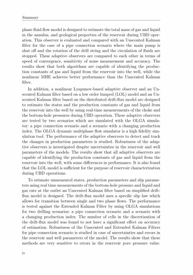
Advanced drilling technologies that are used nowadays utilizes a drillingfluid (mud) which is pumped down through the drill string and flows throughthe drill bit at the bottom of the well (Figure 1.1).
The mud flows up the well annulus carrying cuttings out of the well.The mud is separated at the surface from the return well flow, conditioned,and stored in storage tanks (pits) before it is pumped down into the wellfor further drilling. To avoid fracturing, collapse of the well, or influx offormation fluids surrounding the well, it is crucial to control the pressure inthe open part of the annulus within a certain operating window.
There are three different drilling methods that are commonly used in theindustry namely, conventional drilling (also known as over-balanced drilling),managed pressure drilling (MPD) and under-balanced drilling (UBD). Eachmethod control the pressure in the open part of the annulus differently. Inconventional drilling, this is done by using a mud of appropriate density andadjusting mud pump flow rates. In MPD and UBD, the annulus is sealed,and the mud exits through a controlled choke, allowing for faster and moreprecise control of the annular pressure. In conventional drilling and MPD,the pressure in the well is kept greater than the pressure of the reservoir toprevent influx from entering the well, while in UBD operations the pressureof the well is kept below the pressure of the reservoir, allowing formationfluid flow into the well during the drilling operation.
1.2 Under-balanced Drilling
The first well in Norway drilled with under-balanced techniques was a wellat the Gullfaks field in 2008. The International Association of Drilling Con-tractors (IADC) has defined under-balanced drilling as " A drilling activityemploying appropriate equipment and controls where the pressure exertedin the wellbore is intentionally less than the pore pressure in any part of
4http://news.exxonmobil.com/
2

1.2. Under-balanced Drilling
Figure 1.1: Schematic of a drilling system
the exposed formations with the intention of bringing formation fluids tothe surface" [102]. So, the hydrostatic pressure of the well (pwell) must bekept greater than pressure of collapse (pcoll) and less than both pressure offormation reservoir (pres) and formation fracture pressure (pfrac)
pcoll(t, x) < pwell(t, x) < pres(t, x) < pfrac(t, x) (1.1)
at all times t and positions x. UBD can be classified based on drilling fluidas follows:
� Gas and air drilling� Drilling mud (flow drilling)� Mist drilling� Foam drilling
3
1. Introduction
� Gasified liquid drilling (Gaseated mud)
1.2.1 Gas and air drilling
The gas and air drilling technology is usually used for drilling operationsin low pressure reservoirs and performance drilling operations in compe-tent rock formations [59]. Compressed air, membrane generated Nitrogen,cryogenic Nitrogen, natural gas (hydrocarbon gas), and exhaust gas fromcombustion engines or turbines may be used in gas and air drilling tech-nology. Compressed air is the cheapest and also widely used in mine-shaftsdrilling and water well drilling. But, air could be flammable, explosive andcorrosive. Therefore, air could not be used in hydrocarbon bearing forma-tion. Nitrogen is usually used in UBD operation, notably in offshore drilling.The characteristics of gas and air drilling can be summarized as follows:• High penetration rate
• Low cost
• Good cement job
• Requiring minimal water influx
• Small surface facilityCurrently, air and gas drilling technology is utilized by nearly 30% of land-based oil and natural gas recovery drilling and completion operations[59].
1.2.2 Drilling mud (flow drilling)
Flow drillings are usually suitable for the formation with high hydrostaticpressure. Density of the liquid mud is low enough to satisfy the desired under-balanced conditions. The liquid mud can be used both for water based or oilbased type, and is very similar to the mud used in conventional drilling. Theliquid mud must be an incompressible and homogenous liquid with constantdensity. In addition, it does not have any lost circulation materials (LCM)or bridging materials.
1.2.3 Mist drilling
In the mist drilling, the small quantities of liquid is injected into the gasstream. This method is very similar to the air drilling but the liquid mistassists in cleaning small cuttings around the drill bit. Typical mist mudcomprises less than 2.5% liquid content. The characteristics of mist drillingcan be summarized as follows [59]:• High penetration rate
• Slugging can occur if the ratio of gas and liquid is incorrect
4

1.2. Under-balanced Drilling
• Reduce formation of mud rings
• The mist provides some lubrication to the drill bit
• Since the gas in the mist attenuates the mud pulses of MeasurementWhile Drilling (MWD) system, conventional MWD could not be used,instead an electro-magnetic MWD systems are often used.
1.2.4 Foam drilling
Stable foam has been used by the oil drilling industry since the early 1950s[32, 100]. Stable foam is usually generated by mixing liquid, gas, and surfac-tant foaming agent at surface. Stable foam usually comprises about 55 to 97% gas at surface condition. In a standard deep drilling operation, the mix-ture is injected into the drill string. The surface mixture flows as an aeratedfluid down the drill string to the bottom hole. The foam is formed at thejet nozzles of the drill bit and then flows up the annulus to the surface. Thefoam must be broken into its liquid and gas components at separator. Foamdrilling is a cost effective method for large holes [59]. The characteristics ofstable foam drilling can be summarized as follows:• High carrying capacity
• Low density
• The stable foam can resist during pipe connection or limited circulationstoppages without affecting the removal of cuttings due to the bubblestructures and high fluid yield point
• Reduced pump rates due to improved cuttings transport
• Large surface facility needed
• Since the gas in the stable foam debilitate the mud pulses of MWD sys-tem, conventional MWD could not be used, instead an electro-magneticMWD systems are often used.
• Foam has ability to clean under the bit and the annulus.
1.2.5 Gasified liquid drilling (Gaseated mud)
In this technique, the gas is injected into the incompressible liquid mud toreduce the density. Therefore, gasified liquid drillings are usually suitablefor the formation with low hydrostatic pressure. The mixing can be doneeither on the surface at the base of stand pipe or at the bottom of the well.The gas and liquid mud do not dissolve each other. The liquid mud can useboth water based or oil based type. The multiphase flow of gasified liquiddrilling complicates the hydraulics program. The characteristics of gasifiedliquid drilling can be summarized as follows:
5

1. Introduction
• Lower bottom hole pressures can be achieved
• Less gas volumetric flow rate is required
• Increased amount of surface equipments due to the need to store andcleaning of the base fluid
• Conventional MWD cannot be used when the gas is injected at the topof the drill string
• Slugging can occur if the ratio of gas and liquid is incorrect
1.3 UBD advantages and drawbacks
The automatic UBD has several advantages compared to conventional drillingsuch as increasing the rate of penetration (ROP), increasing the ultimaterecovery from the reservoir, reducing the non-productive time (NPT), re-ducing the risk of differential sticking, reducing the risk of lost circulation,improving the safety and control of the well by using a detailed design forimplementation, increasing the bit life due to requiring less weight on thebit, decreasing/eliminating invasive formation damage, increasing economicbenefits due to flush production during drilling, not exposing shales to mudfiltrate, drilling faster compared to other methods, extending control overBottom-Hole Pressure (BHP) to operational scenarios such as connectionsand trips and when the rig pumps are off, no need to clean up the well af-ter drilling, reducing cutting size and plugging of the rocks in the reservoir,being able to find the most productive zones of the reservoir while drilling,reducing equivalent circulating density (ECD) in extended reach wells, lim-iting or avoiding near well-bore reservoir damage, and reducing drilling-fluidcosts through the use of cheaper, lighter fluid systems [5, 9, 10, 91, 97].
While there are several advantages for UBD systems, there are a fewdrawbacks compared to conventional drilling including: well-bore instabil-ity during UBD, increasing string weight due to reduced buoyancy, discon-tinuous UBD conditions, compatibility with conventional MWD systems,possible abundant borehole erosion, possible increased torque and drag, in-creasing equipment requirement, gravity drainage in horizontal wells, andthe increase cost of personnel due to acquaint with new professions, skills,and procedures [5, 9, 10, 91, 97].
1.4 UBD Equipments and Technology Components
The main surface equipments typically involved in normal UBD operationsare as follows [20, 102]
• Nitrogen unit
6

1.4. UBD Equipments and Technology Components
• Rotating control devices (RCD)
• Chemical injection equipment
• Surface separation equipment
• Choke and manifold system
• Geologic sampler
• Emergency shut-down system
• Non-return valve (NRV)
These components are briefly introduced in the following sections.
1.4.1 Nitrogen unit
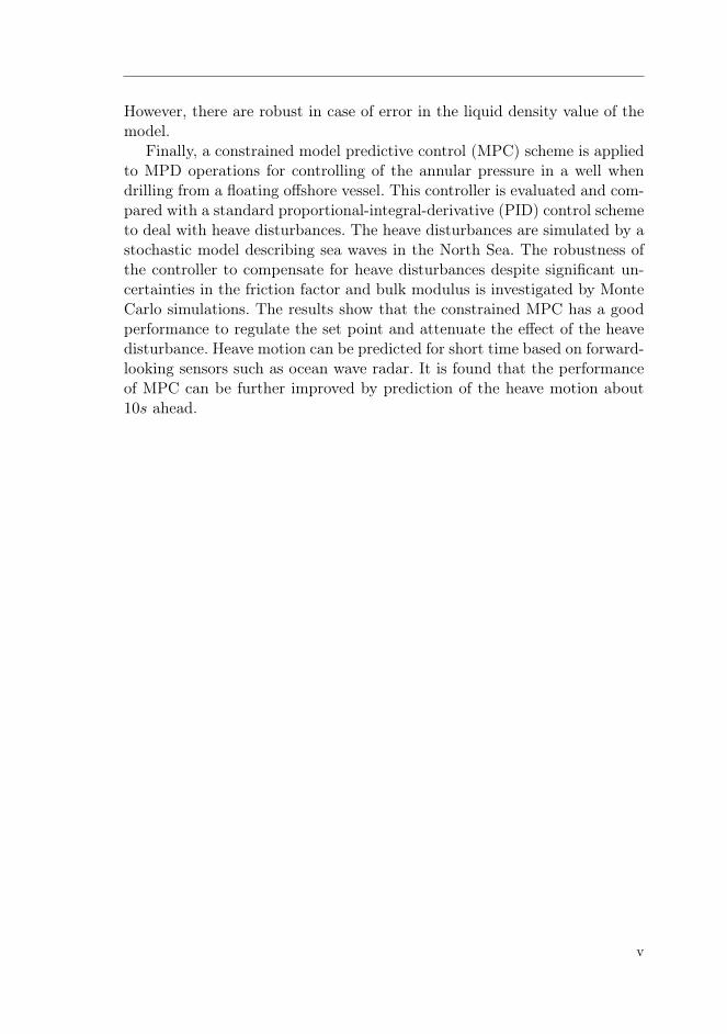
The nitrogen unit provides a supply of high-pressure and high-purity nitro-gen gas for using in typical UBD operations. A nitrogen converter and anitrogen generator are two common types of nitrogen unit. A nitrogen gen-erator is a device that compresses and cools the air and then filters nitrogenout of the air for use in oil or gas wells, and a nitrogen converter is a devicethat converts high pressure liquid nitrogen to high-pressure gas at ambienttemperature. For example,Figure 1.2 shows a high pressure compressor ofnitrogen generation unit.
Figure 1.2: High pressure compressor unit of nitrogen generator (courtesy of Weath-erford International [59] )
7

1. Introduction
1.4.2 Surface separation system
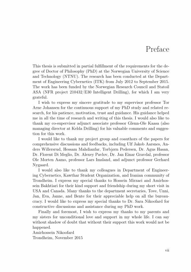
The well fluids contains oil, gas, heavy liquid such as water and drillingmud, and the formation rock cuttings. Therefore, it must be separated bypressurized four (or three) phase separators. The four-phase separator is apressure vessel that separates the well fluids into different phases based ondensity. The heaviest phase is the formation rock cuttings (solids) that fallsdown to the bottom of the separator. The lightest phase is gas that exitsfrom the top of the separator and the oil is stored and evacuated belowthe gas. The heavy liquid is stored and evacuated above the formation rockcuttings. Figure 1.3 shows structure of a four-phase separation system.
Figure 1.3: Structure of a four- phase separator [4]
1.4.3 Rotating control devices (RCD)
Rotating control devices (RCD) are used to seal around the drill string whileallowing rotation of the drill string during UBD operations. It is installed
8

1.4. UBD Equipments and Technology Components
on top of the well. There are two types of RCD [101].
• Passive system: It uses the sealing rubber element and energy fromthe well pressure. It is usually called a Rotating control head.
• Active system: It uses external hydraulic pressure to energize thesealing rubber element. It is usually called a Rotating Annular Preven-ters.
1.4.4 Choke and manifold system
A choke valve is a component that restricts or blocks flow line or orifice.The main function of a choke valve is to adjust the rate of flow and tocontrol the pressure in the well during UBD operations. It is normally usedto control the bottom hole pressure in UBD. The choke manifold consiststwo chokes that can be installed in parallel on a pipe assembly for increasingthe reliability of UBD operation. Figure 1.4 shows the structure of a chokevalve.
Figure 1.4: Structure of a choke valve [17]
9

1. Introduction
1.4.5 Non-return valve (NRV)
The drill pipe Non-Return Valve (NRV) is used to avoid back-flow of drillingfluids from the annulus to the drill pipe. There are two types of NRVs basedon their functions [17].• Bit floats: It is placed at the bottom of the drill pipe above the bit.The functions of the bit floats are safety barrier and shielding themotor, the bit, and MWD against the back flow and plugging by cut-tings [17]. There are different types of bit floats (NRV) such as BasicPiston-Type Float, Hydrostatic Control Valve, Inside BOP (Pump-Down Check Valve), and Retrievable NRV or Check Valve [101].• String floats: It is placed in the drill string and normally 300 metersaway from the surface. It is used to avoid blowing back gas in the drillstring to the drill floor during pipe connection [17].
1.5 Managed Pressure Drilling
The IADC has defined Managed Pressure Drilling as "An adaptive drillingprocess used to precisely control the annular pressure profile throughoutthe wellbore. The objectives are to ascertain the downhole pressure environ-ment limits and to manage the annular hydraulic pressure profile accord-ingly. MPD is intended to avoid continuous influx of formation fluids to thesurface"[101]. In MPD operation, the dynamic pressure of the well must bekept higher than the reservoir pore pressure to prevent gas or formationfluids from entering the well and less than a formation fracture pressure atall times t and positions x.
pres(x) < pwell(x, t) < pfrac(x) (1.2)
The automatic MPD system has several advantages compared to conven-tional drilling as follows [91]:
• Reducing the drilling costs as a result of reducing the nonproductivetime.• Increasing the rate of penetration.• Improving well-bore stability.• Minimizing the risk of lost circulation.• Extending control over bottom-hole pressure (BHP) to operational sce-narios such as connections and trips and when the rig pumps are off.• Improvement in safety and well control resulting from more detaileddesign and planning required for accomplishment.
10

1.6. Background study on UBD operations
1.6 Background study on UBD operations
There are two primary safety barriers in conventional drilling: the mud col-umn (the positive difference between the hydrostatic pressure of the welland the reservoir pressure) and the Blow-Out Preventer (BOP), whereasthe primary safety barrier in UBD operations is the BOP. Since there is nomud column barrier in UBD, it is crucial to pay more attention to controland monitoring of UBD operations.
Since the hydrostatic pressure of the well in UBD operation is intention-ally lower than the reservoir formation pressure, influx fluids (oil, free gasand water) from the reservoir are mixed with rock cuttings and mud fluidin the annulus. Therefore, modeling of the UBD operation should be con-sidered as multiphase flow which can be modeled by a distributed model ora low-order lumped model. Due to the complexity of the multi-phase flow,dynamics of a UBD well coupled with a reservoir, the modeling, estimationand model based control of UBD operations is still considered as an emerg-ing and challenging topic within drilling automation. This section introducesbackground on estimation and control of UBD operations.
1.6.1 Estimation in UBD system
The measurement while drilling (MWD) system in the bottom-hole assembly(BHA) is used to measure and transmit to the surface important informationof the well such as• Bottom-hole pressure
• Hole inclination and azimuth
• Load on the bitThese measurements are normally available in real-time. Logging while
drilling (LWD) is used to measure and store information about properties offormation such as conductivity, porosity, bed thickness, gamma ray, acousticvelocity, etc. [88] Since this data is collected when the tool is pulled out fromthe well, these measurements usually have some delay. Real time knowledgeof geological properties of the reservoir is very useful in many active con-trollers, fault detection systems and safety applications in the well duringpetroleum exploration and production drilling. Therefore, these parametersand states must be estimated online using proper measurements with MWD.Since the selection of a proper model plays the most important role in thesuccess of model based estimators, estimation of states and parameters onUBD operation can be categorized based on the model as follows:
• Estimation based on distributed models
11

1. Introduction
• Estimation based on low-order models
Estimation based on distributed models
Lorentzen et al.[55, 56] designed an ensemble Kalman filter to tune the nineuncertain parameters of a two-phase flow model based on drift flux modelof the UBD operation. This method was applied to synthetic cases and full-scale experimental data. The robustness of the ensemble Kalman filter wasinvestigated by using simulator data with different sets of model parameters.A least squares method was used to tune the uncertain parameters of thetwo-phase flow model instead of the ensemble Kalman filter in [54]. However,it was shown that the least squares approach is not suitable to online tuningdue to more complexity in computation [56].
Vefring et al. [110, 111] compared and evaluated the performance of theensemble Kalman filter and an off-line nonlinear least squares technique uti-lizing the Levenberg-Marquardt optimization algorithm to estimate reservoirpore pressure and reservoir permeability during UBD while performing anexcitation of the bottom-hole pressure. The results show that excitation ofthe bottom-hole pressure might improve the estimation of the reservoir porepressure and reservoir permeability.
Aarsnes et al. [2] introduced a simplified drift-flux model and estima-tion of the distributed multiphase dynamics during UBD operation. Thismodel used a specific empirical slip law without flow-regime predictions .The estimation algorithm separates varying parameters slowly and poten-tially changing parameters more quickly such as the PI (this sentence is veryhard to read think more about it). In this model, fast changing parameterswere estimated online simultaneously with the states of the model, whileother parameters were calibrated infrequently and offline.
Di Meglio et al. designed an adaptive observer based on a back steppingapproach for a linear first-order hyperbolic system of Partial DifferentialEquations (PDEs) by using only boundary measurements with applicationto UBD [15]. It was shown that this method has exponential convergence forthe distributed state and the parameter estimation. This adaptive observerwas used to estimate distributed states and unknown boundary parametersof the well during UBD operations.
Gao Li et al. presented an algorithm for characterizing reservoir porepressure and reservoir permeability during UBD of horizontal wells [51, 52].Since the total flow rate from the reservoir has a negative linear correlationwith the bottom hole pressure, reservoir pore pressure was identified bythe crossing of the horizontal axis and the best-fit regression line betweenthe total flow rate from the reservoir and the bottom hole pressure whileperforming an excitation of the bottom-hole pressure by changing the choke
12

1.6. Background study on UBD operations
valve opening or pump rates. The results show a reasonable performance forthis method for reservoir characterization in horizontal well.
Estimation based on low-order models
Nygaard et al. compared and evaluated the performance of the extendedKalman filter, the ensemble Kalman filter and the unscented Kalman filterbased on a low order model to estimate the states and the production index(PI) in UBD operation [82]. The results show that the unscented Kalmanfilter has a better performance than other methods.
Nazari et al. [69] designed and compared the performance of the ensembleKalman filter and the unscented Kalman filter based on a low order modeldeveloped in [80] to estimate the states. For extracting more reliable infor-mation from several pressure sensors at each moment, two centralized anddistributed estimation fusion schemes based on the unscented Kalman filterfor estimating and monitoring mixture velocity of drill-string and annuluswas developed. The result of central estimation fusion method was more ac-curate than the distributed estimation fusion method. But, the distributedfusion presented more robust results.
Reservoir characterization in Under-Balanced Drilling
As mentioned above, reservoir characterization can be estimated by usingboth low-order models and distributed models. Real-time updates of reser-voir properties which are part of these models are able to improve efficiencyof the overall well construction by calculating reservoir characterization ac-curately while drilling, ultimately enabling increased oil recovery by betterwell completion.Reservoir characterization during UBD has been investigated by severalresearchers[39, 41, 52, 110, 111], focusing mainly on the estimation of thereservoir pore pressure and reservoir permeability by using the assumptionthat the total flow rate from the reservoir is known [110]. Since the totalflow rate from the reservoir is usually unknown or unmeasurable online,this thesis has designed novel methods to estimate reservoir properties withonly pressure measurements.This can highly improve safety and efficiencyof UBD operations.
13

1. Introduction
1.6.2 Control in UBD system
In oil and gas drilling operations, the main goal of automatic or manualcontroller is to control the annulus pressure in the well under both staticand dynamic conditions. In addition, an other objective of well control inUBD operations is to control influx of formation fluids. The most importantmanipulated variables for control in UBD operations are the choke valveopening, drilling fluid density and the drilling fluid injection flow rates.These variables have different time-scales and effects on UBD operations.The choke valve opening is generally used to control the rapid pressure fluc-tuations during the UBD operations. The other manipulated variables canbe used to adjust pressure and friction in the well for long time scale.
Perez Tellez et al. [94, 95]proposed UBD flow control procedure based ona mechanistic model for control of the bottom-hole pressure and influx offormation fluids during routine operation and pipe connections procedures.The mechanistic model was validated with both field measurements froma Mexican well and full-scale experimental data. Manipulated variables inthis controller were the choke valve opening and the drilling fluid injectionflow rates. In this study, the choke valve is adjusted manually based on thecalculated set-point. This method can cause some errors if the planned pipeconnection is not performed properly
Nygaard et al.[81] designed a nonlinear model predictive control(NMPC)based on a detailed model for regulating bottom-hole pressure during thedrilling operations and pipe connections procedures. This controller wascompared by two other control algorithms, a PI controller with feed-forwardcontrol of the pump rates and a manual controller. The PI scheme parame-ters were tuned by Ziegler-Nichols closed loop algorithm based on a low-ordermodel. The performance of all algorithms was tested on the detailed model.The results showed that the nonlinear model predictive control has a betterperformance than the PI and the manual controller.
Nygaard et al. [84, 87] used a nonlinear model predictive control algo-rithm based on detailed model to obtain optimal choke pressure and pumprate for controlling the bottom-hole pressure during pipe connection in a gasdominant well. They used the unscented Kalman filter for nonlinear modelto estimate the states, and the permeability of the reservoir. The reservoirwas divided into three zones, and the permeability of the reservoir for eachzone was estimated. The results show that this control algorithm can reducefluctuations in the bottom hole pressure during UBD operations.
In Nygaard et al. [85], a finite horizon nonlinear model predictive controlin combination with an unscented Kalman filter was designed for controllingthe bottom-hole pressure based on a low order model developed in [81]. Inthis study the unscented Kalman filter (UKF) was used to estimate the
14

1.7. Background on control of heave disturbance in offshore MPD
states, and the friction and choke coefficients.
1.7 Background on control of heave disturbance in offshoreMPD
There is a specific disturbance occurring during drilling from floaters thatsignificantly affects MPD operations. In this case, the rig moves verticallywith the waves, referred to as heave motion. As drilling proceeds, the drillstring needs to be extended with new sections. Thus, every couple of hoursor so, drilling is stopped to add a new segment of about 27 m to the drillstring. During drilling, a heave compensation mechanism is active to isolatethe drill string from the heave motion of the rig. However, during connec-tions, the pump is stopped, and the string is disconnected from the heavecompensation mechanism and rigidly connected to the rig. The drill stringthen moves vertically with the heave motion of the floating rig and acts likea piston on the mud in the well. The heave motion may be more than 3m in amplitude and typically has a period of 10–20 s, which causes severepressure fluctuations at the bottom of the well. Pressure fluctuations havebeen observed to be an order of magnitude higher than the standard limitsfor pressure regulation accuracy in MPD (about ±2.5 bar) [24]. Downwardmovement of the drill string into the well increases pressure (surging), andupward movement decreases pressure (swabbing). Excessive surge and swabpressures can lead to mud loss resulting from high-pressure fracturing of theformation or a kick-sequence (uncontrolled influx from the reservoir) thatcan potentially grow into a blowout as a consequence of low pressure.
Rasmussen et al.[99] compared and evaluated different MPD methods forthe compensation of surge and swab pressure. In Nygaard et al. [86], it isshown that surge and swab pressure fluctuation in the BHP during pipe con-nection can be suppressed by controlling the choke and main pump. Nygaardet al. [87] used a nonlinear model predictive control (MPC) algorithm to ob-tain optimal choke pressure for controlling the BHP during pipe connectionin a gas-dominant well. Pavlov et al. [93] presented two nonlinear controlalgorithms for handling heave disturbances in MPD operations. Mahdianfaret al. [61, 62] designed an infinite-dimensional observer that estimates theheave disturbance. This estimation is used in a controller to reject the effectof the disturbance on the downhole pressure. In all the above mentionedpapers, the controllers are designed for the nominal case disregarding theuncertainty in the parameters, although several parameters in the well couldbe uncertain during drilling operations. In addition, the heave disturbance,which is inherently stochastic and contains many different spectral harmon-ics, is approximated by one or a couple of sinusoidal waves with known fixed
15

1. Introduction
frequencies throughout controller design and simulations [50]. In this the-sis, a stochastic model for the heave motion in the North Sea is given andused in simulations. This thesis develops a model predictive controller forthe first time to control the annular pressure in a well to deal with heavedisturbances during offshore MPD operations. This can improve safety andperformance of MPD operations.
1.8 Research Objective
Based on background studies, the main research objective of this thesis isto develop methods using both distributed and low order model to estimatethe states and geological properties of the reservoir during UBD operations.Since reservoir properties determine anticipated influx of formation fluidsduring UBD operations, reservoir characterization has important role inthe safety and efficiency of UBD technology. Real-time updates of reser-voir properties may improve efficiency of the overall well construction byaccurate estimation of reservoir characterization while drilling. And conse-quently, enabling increased oil recovery by better well completion.
Since heave motion in offshore drilling induces severe pressure fluctua-tions at the bottom of the well, improper control leads to loss of mud, rigblowout and formation kicks. Therefore, in this work it has been developedalgorithms to control the annular pressure in a well to deal with heave dis-turbances during offshore MPD operations. In some cases, short-term heavemotion can be predicted based on forward-looking sensors such as oceanwave radar and used directly in MPC controller. Short-term heave motionprediction can also improve performance of MPC to deal with heave distur-bance.
1.9 Summaries and Outline of the Thesis
Advancement of automation on drilling technologies solved quite a few chal-lenges in this sector in the past few decades. However, still there are manymore challenges that has to be addressed. This work addresses two of theimportant challenges that drilling technology faces nowadays :
1. Accurate reservoir characterization in UBD
2. Control of heave disturbance in offshore MPD operationsTo solve these challenges, this thesis includes novel solutions. The summaryof contributions of each chapter is as follows. Each of the following chaptersis based on a number of papers that are published independently, or sub-
16

1.9. Summaries and Outline of the Thesis
mitted for publication:
Chapter 2. Nonlinear Moving Horizon Observer for estimationof states and parameters in Under-Balanced drilling operations:This chapter describes a nonlinear Moving Horizon Observer to estimate theannular mass of gas and liquid, and production constants of gas and liquidfrom the reservoir into the well during UBD operations with measuring thechoke pressure and the bottom-hole pressure. This observer algorithm whichis based on a low-order lumped model is evaluated against Joint UnscentedKalman filter for two different simulations with low and high measurementnoise covariance. The results show that both algorithms are capable of iden-tifying the production constants of gas and liquid from the reservoir into thewell, while the nonlinear Moving Horizon Observer achieves better perfor-mance than the Unscented Kalman filter. A version of the contents of thischapter was presented in [74].
Chapter 3. Reservoir characterization in Under-balanced Drillingusing Low-Order Lumped Model: Estimation of the production indexof oil and gas from the reservoir into the well during UBD operations isstudied. This chapter compares a Lyapunov-based adaptive observer and ajoint unscented Kalman filter (UKF) based on a low order lumped (LOL)model and the joint UKF based on the distributed drift-flux model by usingreal-time measurements of the choke and the bottom-hole pressures. Usingthe OLGA simulator, it is found that all adaptive observers are capable ofidentifying the production constants of gas and liquid from the reservoir intothe well, with some differences in performance. The results show that theLOL model is sufficient for the purpose of reservoir characterization dur-ing UBD operations. Robustness of the adaptive observers is investigated incase of uncertainties and errors in the reservoir and well parameters of themodels. A version of the contents of this chapter has been submitted in [79],based on preliminary results in [73] and [78].
Chapter 4. State and parameter estimation of a Drift-Flux Modelfor Under-Balanced Drilling operations: This chapter presents a drift-flux model describing multiphase (gas-liquid) flow during drilling. The drift-flux model uses a specific slip law which allows for transition between singleand two phase flows.With this model, we design an Unscented and ExtendedKalman Filters (UKF and EKF) for estimation of unmeasured states andproduction and slip parameters using real time measurements of the bottom-hole pressure and pressure and flow-rates at the outlet. The OLGA high-fidelity simulator is used to create two scenarios from UBD operations on
17

1. Introduction
which the estimators are tested: A pipe connection scenario and a scenariowith a changing production index. A performance comparison reveal thatboth UKF and EKF are capable of identifying the production constants ofgas from the reservoir into the well with sufficient accuracy, while the UKFis more accurate than the EKF. Robustness of the UKF and EKF for thepipe connection scenario is studied in case of uncertainties and errors in thereservoir and well parameters of the model. It is found that these methodsare very sensitive to errors in the reservoir pore pressure value. However,there are robust in case of error in the liquid density value of the model. Aversion of the contents of this chapter has been submitted in [77], based onpreliminary results in [76].
Chapter 5. Design constrained MPC for heave disturbance at-tenuation in offshore Managed Pressure drilling systems: This chap-ter presents a constrained finite horizon model predictive control (MPC)scheme for regulation of the annular pressure in a well during managedpressure drilling from a floating vessel subject to heave motion. In additionto the robustness of a controller, the methodology to deal with heave distur-bances despite uncertainties in the friction factor and bulk modulus is inves-tigated. The stochastic model describing sea waves in the North Sea is usedto simulate the heave disturbances. The results show that the closed-loopsimulation without disturbance has a fast regulation response, without anyovershoot, and is better than a proportional-integral-derivative controller.The constrained MPC for managed pressure drilling shows further improveddisturbance rejection capabilities with measured or predicted heave distur-bance. Monte Carlo simulations show that the constrained MPC has a goodperformance to regulate set point and attenuate the effect of heave distur-bance in case of significant uncertainties in the well parameter values. Aversion of the contents of this chapter was presented in [75], based on pre-liminary results in [72].
Chapter 6. Conclusions. This chapter presents main conclusions ofthis thesis and possible future research directions.
1.10 Main Contributions
The main contributions of this work can be summarized as follows:
� Nonlinear Moving Horizon Observer using a Low-Order Lumped modelfor estimation of states and parameters in UBD operations, chapter 2.
18

1.11. Publications
� The proof of stability of Lyapunov-based adaptive observer based on aLow-Order Lumped model for estimation of Production Index in UBDoperations, chapter 3.
� Comparasion of the joint unscented Kalman filter and a Lyapunov-based adaptive observer for estimating the states and production con-stant of gas and liquid from the reservoir into the well based on aLow-Order Lumped model for UBD operation, chapter 3.
� Applying the unscented Kalman Filter for estimation of states andparameters of a Drift-Flux Model, chapters 3 & 4.
� Constrained model predictive control (MPC) scheme for regulation ofthe annular pressure in a well and heave disturbance attenuation inoffshore MPD systems, chapter 5.
1.11 Publications
The main contribution of this thesis presented in several conferences andjournal papers which are listed below:
• Nikoofard, A., Johansen, T. A., Mahdianfar, H., and Pavlov, A.(2013, June). Constrained MPC design for heave disturbance attenua-tion in offshore drilling systems. In OCEANS-Bergen, 2013 MTS/IEEE(pp. 1-7). IEEE.
• Nikoofard, A., Johansen, T. A., Mahdianfar, H., and Pavlov, A.(2014). Design and comparison of constrained MPC with pid controllerfor heave disturbance attenuation in offshore managed pressure drillingsystems. Marine Technology Society Journal, 48(2), 90-103.
• Nikoofard, A., Johansen, T. A., and Kaasa, G. O. (2014, June). De-sign and comparison of adaptive estimators for Under-Balanced Drilling.In American Control Conference (ACC), 2014 (pp. 5681-5687). IEEE.
• Nikoofard, A., Johansen, T. A., and Kaasa, G. O. (2014, October).Nonlinear Moving Horizon Observer for Estimation of States and Pa-rameters in Under-Balanced Drilling Operations. In ASME 2014 Dy-namic Systems and Control Conference (pp. V003T37A002-V003T37A002).American Society of Mechanical Engineers.
• Nikoofard, A., Aarsnes, U. J. F., Johansen, T. A., and Kaasa, G.O. (2015, May). Estimation of States and Parameters of a Drift-FluxModel with Unscented Kalman Filter. In Proceedings of the 2015 IFACWorkshop on Automatic Control in Offshore Oil and Gas Production(Vol. 2, pp. 171-176).
19

1. Introduction
• Nikoofard, A., Johansen, T. A., and Kaasa, G. O. (2015, June).Evaluation of Lyapunov-based Adaptive Observer using Low-OrderLumped Model for Estimation of Production Index in Under-balancedDrilling. In Proceedings of 9th IFAC international symposium on ad-vanced control of chemical processes (pp. 69-75)
• Nikoofard, A., Johansen, T. A., and Kaasa, G. O. Reservoir charac-terization in Under-balanced Drilling using Low-Order Lumped Model.Journal of Process Control (submitted)
• Nikoofard, A., Aarsnes, U. J. F., Johansen, T. A., and Kaasa, G.O. State and Parameter Estimation of a Drift-Flux Model for Under-Balanced Drilling Operations. IEEE Transactions Control Systems Tech-nology (submitted)
20

CHAPTER2Nonlinear Moving Horizon Observer forestimation of states and parameters in
Under-Balanced drilling operations
2.1 Introduction
In recent years there has been increasing interest in Under-Balanced Drilling(UBD). UBD has the potential to both decrease drilling problems and im-prove hydrocarbon recovery. In conventional (over-balanced) drilling, or Man-aged Pressure Drilling (MPD), the pressure of the well must be kept greaterthan pressure of reservoir to prevent influx from entering the well. But in anUBD operation, the hydrostatic pressure in the circulating downhole fluidsystem must be kept greater than pressure of collapse and less than pressureof reservoir
pcoll(t, x) < pwell(t, x) < pres(t, x) (2.1)
at all times t and positions x. Since hydrostatic pressure in the circulatingdownhole fluid system is intentionally lower than the reservoir formationpressure, influx fluids (oil, free gas, water) from the reservoir are mixed withrock cuttings and drilling fluid (“mud") in the annulus. Therefore, modelingof the UBD operation should be considered as multiphase flow. Differentaspects of modeling relevant for UBD have been studied in the literature[19, 47, 81, 106].
Estimation and control design in MPD has been investigated by severalresearchers [38, 63, 72, 75, 92, 105, 113, 114]. However, due to the complexityof multi-phase flow dynamics in UBD operations, there are few studies onestimation and control of UBD operations [56, 73, 81, 82, 85]. Nygaard etal. [82] compared and evaluated the performance of the extended Kalmanfilter, the ensemble Kalman filter and the unscented Kalman filter to esti-
21

2. Nonlinear Moving Horizon Observer for estimation of states and parametersin Under-Balanced drilling operations
mate the states and production index in UBD operation. Lorentzen et al.[56]designed an ensemble Kalman filter to tune the uncertain parameters of atwo-phase flow model in the UBD operation. In Nygaard et al [85], a finitehorizon nonlinear model predictive control in combination with an unscentedKalman filter was designed for controlling the bottom-hole pressure basedon a low order model developed in [81], and the unscented Kalman filterwas used to estimate the states, and the friction and choke coefficients. GaoLi et al. presented an algorithm for characterizing reservoir pore pressureand reservoir permeability during UBD of horizontal wells [51, 52]. Sincethe total flow rate from the reservoir has a negative linear correlation withthe bottom hole pressure, reservoir pore pressure can be identified by thecrossing of the horizontal axis and the best-fit regression line between thetotal flow rate from the reservoir and the bottom hole pressure while per-forming an excitation of the bottom-hole pressure by changing the chokevalve opening or pump rates. Nikoofard et al.[73] designed Lyapunov-basedadaptive observer, recursive least squares and joint unscented Kalman filterbased on a low-order lumped model to estimate states and parameters duringUBD operations by using the total mass of gas and liquid as measurementscalculated from pressure measurements using a model. The performance ofadaptive estimators are compared and evaluated for two cases.The resultsshow that all estimators were capable of identifying the production constantsof gas and liquid from the reservoir into the well, while the Lyapunov basedadaptive observer had the best performance comparing with other methodswhen there was a significant amount of noise. This chapter estimates statesand parameters only by using real-time measurements of the choke and thebottom-hole pressures.
Due to mathematical complexity presented by nonlinearity, state and pa-rameter estimation of nonlinear dynamical systems is one of the challengingtopics in the control theory and has been the subject of many studies sinceits advent. The adaptive observer was proposed by Carrol et al. in 1973[14]. The Lyapunov based adaptive observer is generally used to design aLuenberger type observer for the state while appropriate adaptive law toestimate the unknown parameters [33, 43, 68, 71]. If the observability andpersistency excitation condition is satisfied, then both the state and theparameter estimation will converge to their true values. Nonlinear MovingHorizon Estimation is one of the powerful method which estimates statesand parameters simultaneously [34, 65, 98]. At each sampling time, a Mov-ing Horizon Estimation estimate the state and parameter by minimizing acost function over the previous finite horizon, subject to the nonlinear modelequations. Robustness to lack of persistent excitation and measurement noiseis due to the use of an apriori prediction model as well as some modifications
22

2.2. Modeling
to the basic MHE algorithm [35, 107]. The original Kalman filter based onlinear model was developed to estimate both state and parameter of thesystem usually known as an augmented Kalman filter. Several Kalman fil-ter techniques have been developed to work with non-linear system. Theunscented Kalman filter has been shown to have a better performance thanother Kalman filter techniques for nonlinear system in same cases [104, 112].
Total mass of gas and liquid in the well could not be measured directly,as well as some geological properties of the reservoir such as productionconstants of gas and liquid from the reservoir might vary and could be un-certain during drilling operations. Therefore, they must be estimated byadaptive estimators during UBD operations. It is assumed that the bottom-hole pressure (BHP) readings are transmitted continuously to the surfacethrough a wired pipe telemetry with a pressure sensor at the measurementwhile drilling (MWD) tool [31]. This chapter presents the design of a non-linear Moving Horizon Estimation based on a nonlinear two-phase fluid flowmodel to estimate the total mass of gas and liquid in the annulus and geo-logical properties of the reservoir during UBD operation. The performanceof this methods is evaluated against Joint Unscented Kalman Filter for thecase of pipe connection operations where the main pump is shut off andthe rotation of the drill string and the circulation of fluids are stopped. Theestimators are compared to each other in terms of speed of convergence,sensitivity of noise measurement, and accuracy.
This chapter consists of the following sections: The modeling sectionpresents a low-order lumped model based on mass and momentum balancesfor UBD operation. The adaptive observer section explains nonlinear Mov-ing Horizon Estimation for simultaneously estimating the states and modelparameters of a nonlinear system from noisy measurements. In the Simu-lations section, the simulation results are provided for state and parameterestimation. At the end, the conclusion that has been made through thischapter are presented.
2.2 Modeling
Modeling of Under-balanced Drilling (UBD) in an oil well is a challengingmathematical and industrial research area. Due to existence of multiphaseflow (i.e. oil, gas, drilling mud and cuttings) in the system, the modelingof the system is very complex. Multiphase flow can be modeled as a dis-tributed (infinite dimension) model or a lumped (finite dimension) model.A distributed model is capable of describing the gas-liquid behavior alongthe annulus in the well. In this chapter, a low-order lumped (LOL) modelis used. The lumped model considers only the gas-liquid behavior at the
23

2. Nonlinear Moving Horizon Observer for estimation of states and parametersin Under-Balanced drilling operations
drill bit and the choke system. This modeling method is very similar to thetwo-phase flow model found in [1, 81]. The simplifying assumptions of theLOL model are listed as below:
� Ideal gas behavior
� Simplified choke model for gas, mud and liquid leaving the annulus
� No mass transfer between gas and liquid
� Isothermal condition and constant system temperature
� Constant mixture density with respect to pressure and temperature.
� Liquid phase considers the total mass of mud, oil, water, and rock cut-tings.
The simplified LOL model equations for mass of gas and liquid in anannulus are derived from mass and momentum balances as follows
mg = wg,d + wg,res(mg,ml)−mg
mg +mlwout(mg,ml) (2.2)
ml = wl,d + wl,res(mg,ml)−ml
mg +mlwout(mg,ml) (2.3)
where mg and ml are the total mass of gas and liquid, respectively. Theliquid phase is considered incompressible, and ρl is the liquid mass density.The gas phase is compressible and occupies the space left free by the liquidphase. wg,d and wl,d are the mass flow rate of gas and liquid from the drillstring, wg,res and wl,res are the mass flow rates of gas and liquid from thereservoir. The total mass outflow rate is denoted by wout.
The total mass outlet flow rate is calculated by the valve equation
wout = KcZ
√mg +ml
Va
√pc − pc0 (2.4)
where Kc is the choke constant. Z is the control signal to the choke opening,taking its values on the interval (0, 1]. The total volume of the annulus isdenoted by Va. pc0 is the constant downstream choke pressure (atmospheric).The choke pressure is denoted by pc, and derived from ideal gas equation
pc =RT
Mgas
mg
Va − mlρl
(2.5)
where R is the gas constant, T is the average temperature of the gas, andMgas is the molecular weight of the gas. The flow from the reservoir intothe well for each phase is commonly modeled by the linear relation with the
24

2.3. Adaptive Observer
pressure difference between the reservoir and the well. The mass flow ratesof gas and liquid from the reservoir into the well are given by
wg,res =
{Kg(pres − pbh), if pres > pbh
0, otherwise.(2.6)
wl,res =
{Kl(pres − pbh), if pres > pbh
0, otherwise.(2.7)
where pres is the known pore pressure in the reservoir, and Kg and Kl
are the production constants of gas and liquid from the reservoir into thewell, respectively. Finally, the bottom-hole pressure is given by the followingequation
pbh = pc +(mg +ml)g cos(∆θ)
A+ ∆pf (2.8)
where g is the gravitational constant, A is the cross sectional area of theannulus, ∆θ is the average angle between gravity and the positive flow di-rection of the well, ∆pf is the friction pressure loss in the well
∆pf = Kf (wg,d + wl,d)2 (2.9)
and Kf is the friction factor.Reservoir parameters could be evaluated by seismic data and other geo-
logical data from core sample analysis. But, local variations of reservoir pa-rameters such as the production constants of gas and liquid may be revealedonly during drilling. So, it is valuable to estimate the partial variations ofsome of the reservoir parameters while drilling is performed [82].
2.3 Adaptive Observer
In this section, first the Nonlinear Moving Horizon Estimation (MHE) toestimate states and parameters in UBD operation is explained. Then, thejoint unscented Kalman filter is presented for same problem.The choke andthe bottom-hole pressures are outputs and measurements of the system. Themeasurements and inputs of the observer are summarized in Table 2.1. Theproduction constant of gas (Kg) and liquid (Kl) from the reservoir into thewell are unknown and must be estimated. Below Kg and Kl are denoted byθ1 and θ2, respectively.
25

2. Nonlinear Moving Horizon Observer for estimation of states and parametersin Under-Balanced drilling operations
Table 2.1: Measurements and Inputs
Variables TypeChoke pressure (pc) MeasurementBottom-hole pressure (pbh) MeasurementDrill string mass flow rate of gas (wg,d) InputDrill string mass flow rate of liquid (wl,d) InputChoke opening (Z) Input
2.3.1 Nonlinear Moving Horizon Estimation
The LOL model based on equations (2.2)-(2.3) can be represented by adiscrete explicit scheme given by
xk = f(xk−1, uk−1) + qk (2.10)yk = h(xk) + rk (2.11)
h(xk) = [pc, pbh]T (2.12)
where qk and rk are the process noise and the measurement noise, and uk isthe input. At time t, the information vector of the N + 1 last measurementsand the N last inputs is defined as
It = col(yt−N , ..., yt, ut−N , ..., ut−1) (2.13)
N + 1 is the finite horizon or window length . This information can besummarized in a single vector for measurement and input as follow
Yt =
yt−Nyt−N+1
...yt
Ut =
ut−Nut−N+1
...ut−1
(2.14)
Nonlinear MHE cost function can be considered as follows
J(xt−N,t, xt−N,t, It) = ‖W (Yt −Ht(xt−N,t))‖2 + ‖V (xt−N,t − xt−N,t)‖2(2.15)
where V,W are the positive definite weight matrices. Choosing the tuningmatrices V,W in the MHE specify trade-offs in the MHE design. Choosingsmall tuning matrices V,W lead to faster track of data and convergencebut more uncertainty in the estimation. Choosing larger tuning matrices Wand V lead to slower track of data and convergence but less uncertainty inthe estimation. The cost function (2.15) consists of two standard terms: one
26

2.3. Adaptive Observer
is a term that penalizes the deviation between the measured and predictedoutputs, the other term weights the difference between the estimated state atthe start of the horizon from its prediction. The Nonlinear MHE minimizesthe cost function (2.15) over the window of the current measurement andthe historical measurement, subject to the nonlinear model equations. xot−N,tis the optimal solution of this problem.The sequence of the state estimatesxi,t (i = t − N, . . . , t) can be yielded from the noise free nonlinear modeldynamics. So, a sequence of denoted as estimated output vectors Yt can beformulated as follows
Yt = H(xt−N,t, Ut) = Ht(xt−N,t) =
h(xt−N,t)
h(fut−N (xt−N,t))...
h(fut−1(. . . (fut−N (xt−N,t))))
(2.16)
A one-step prediction xt−N,t is determined from xot−N−1,t−1 as follow
xt−N,t = f(xot−N−1,t−1, ut−N−1) t = N + 1, N + 2, . . . (2.17)
For parameter estimation, x is augmented with the unknown parametervector θ with the dynamic model θt+1 = θt.
2.3.2 Joint Unscented Kalman Filter
The Unscented Kalman Filter (UKF) was introduced in [36, 37, 109]. Themain idea behind the method is that approximation of a Gaussian distribu-tion is easier than approximation on of an arbitrary nonlinear function. TheUKF estimates the mean and covariance matrix of estimation error witha minimal set of sample points (called sigma points) around the mean byusing a deterministic sampling approach known as the unscented transform.The nonlinear model is applied to sigma points instead of a linearization ofthe model. So, this method does not need to calculate explicit Jacobian orHessian. More details can be found in [36, 104, 109, 112].
Two common approaches for estimation of parameters and state vari-ables simultaneously are dual and joint UKF techniques. The dual UKFmethod uses another UKF for parameter estimation so that two filters runsequentially in every time step. At each time step, the state estimator up-dates with new measurements, and then the current estimate of the state isused in the parameter estimator. The joint UKF augments the original statevariables with parameters and a single UKF is used to estimate augmentedstate vector. The joint UKF is easier to implement [109, 112].
Using the joint UKF, the augmented state vector is defined by xa =[X, θ]. The state-space equations for the the augmented state vector at time
27

2. Nonlinear Moving Horizon Observer for estimation of states and parametersin Under-Balanced drilling operations
instant k is written as:x1,kx2,kθ1,kθ2,k
=
f1(Xk−1, θ1,k−1)f2(Xk−1, θ2,k−1)
θ1,k−1θ2,k−1
= fa(Xk−1, θk−1, uk−1) + qk (2.18)
mg and ml are denoted by x1 and x2, respectively. The discrete measure-ments of the system can be modeled as follows:
yk = h(Xk) + rk (2.19)
h(Xk) = [pc, pbh]T (2.20)
where rk ∼ N(0, Rk) is the zero mean Gaussian measurement noise.
2.4 Simulation Results
The parameter values for the simulated well, LOL model and reservoir aresummarized in Table 2.2. These parameters are used from the offshore test ofWeMod simulator[89]. WeMod is a high fidelity drilling simulator developedby the International Research Institute of Stavanger (IRIS). In WEMOD,the drift-flux model was used for modeling one-dimensional two-phase flowin well. To derive thermodynamic relations, it is generally assumed a systemin thermodynamic equilibrium (PVT-models), ideal gas law, and a moredetailed model for mud PVT properties[89]. The process noise covariancematrix used in this plant model (LOL model) is
Q = diag[10−1, 10−1, 10−4, 10−4]
UKF parameters are determined empirically and used in the series ofequations presented in the Appendix.A. The parameter values for nonlinearMHE and joint UKF are summarized in Table 2.3.
The time-step used for discretizing the dynamic model and adaptive es-timator was 1 seconds. The initial values for the estimated and real statesand parameters are as follows
x1 = 5446.6, x2 = 54466.5, θ1 = 5 , θ2 = 5
x1 = 4629.6, x2 = 46296.2, θ1 = 4.25, θ2 = 4.25
The scenario in this simulation is as follows, first the drilling in a steady-state condition is initiated, then at t = 10 min the main pump is shut offto perform a connection procedure. The rotation of the drill string and thecirculation of fluids are stopped for 10 mins. Next after making the first pipe
28

2.4. Simulation Results
Table 2.2: Parameter Values for Well and Reservoir
Name LOL UnitReservoir pressure (pres) 270 barCollapse pressure (pcoll) 255 barFriction pressure loss (∆pf ) 10 barWell total length (Ltot) 2300 mWell vertical depth (L) 1720 mDrill string outer diameter (Dd) 0.1397 mAnnulus volume (Va) 252.833 m3
Annulus inner diameter (Da) 0.2445 mLiquid flow rate (wl,d) 44 Kg/sGas flow rate (wg,d) 5 Kg/sLiquid density (ρl) 1475 Kg/m3
Production constant of gas (Kg) 5× 10⁻⁶ Kg/PaProduction constant of liquid (Kl) 5× 10⁻⁵ Kg/PaGas average temperature (T ) 25 ◦CAverage angle (∆θ) 0.726 radChoke constant (Kc) 0.013 m2
Table 2.3: Parameter Values for Estimators
Parameter Value Parameter ValueW 100 V diag (0.1,0.1, 0.03, 0.05)N + 1 15 κ 0β 2 α 0.5
connection at t = 20 min the main pump and rotation of the drill string arerestarted. Then at t=52 min the second pipe connection procedure is started,and is completed after 12 mins. Two different simulations with low and highmeasurement noise covariances are performed. In the first simulation, thechoke and the bottom-hole pressures measurements are corrupted by zeromean additive white noise with the following covariance matrix
R = diag[0.52, 0.52]
Figures 2.1 and 2.2 show the measured and estimated total mass of gasand liquid, respectively. The nonlinear MHE is more accurate than UKF toestimate the total mass of gas and liquid. The estimation of the productionconstants of gas and liquid from the reservoir into the well are shown inFigures 2.3 and 2.4, respectively. In estimation of the production constantsof gas and liquid from the reservoir into the well, nonlinear MHE has a veryfast convergence rate, about 30 seconds or less. UKF take much longer and
29

2. Nonlinear Moving Horizon Observer for estimation of states and parametersin Under-Balanced drilling operations
it is in the order of minutes. After convergence to the value, the correctnonlinear MHE has more small fluctuations than UKF for estimation of theproduction constants of gas and liquid.
0 20 40 60 80 100 1205460
5470
5480
5490
5500
5510
5520
5530
5540
5550
5560
Time (min)
Ma
ss (
kg
)
Total mass of gas
Nonlinear MHE
Real system
UKF
Figure 2.1: Total mass of gas with the low measurement noise covariance
In second simulation, the choke and the bottom-hole pressures are cor-rupted by zero mean additive white noise with the following covariance ma-trix
R = diag[502, 502]
Figures 2.5 and 2.6 show the measured and estimated total mass of gas andliquid, respectively. It is found that the nonlinear MHE is more accuratethan UKF to estimate the total mass of gas and liquid. The estimation ofthe production constants of gas and liquid from reservoir into the well are il-lustrated in Figures 2.7 and 2.8, respectively. In estimation of the productionconstants of gas and liquid from the reservoir into the well, the nonlinearMHE has a very fast convergence rate, about 30 seconds or less, while theUKF takes almost 7 minutes.
In this section, performance of these adaptive estimators is evaluatedthrough the root mean square error (RMSE) metric. The RMSE metric fornonlinear MHE and UKF in two cases are summarized in Table 2.4.
30

2.4. Simulation Results
0 20 40 60 80 100 120
5.2
5.25
5.3
5.35
5.4
5.45
x 104
Time (min)
Ma
ss (
kg
)
Total mass of liquid
Nonlinear MHE
Real system
UKF
Figure 2.2: Total mass of liquid with the low measurement noise covariance
0 2 4 6 8 10 12 14 16 18 204.2
4.4
4.6
4.8
5
5.2
5.4
5.6
Time (min)
Kg (
kg
/s/1
0b
ar)
Estimation of Kg
Nonlinear MHE
Real parameter
UKF
Figure 2.3: Production constant of gas with the low measurement noise covariance
31

2. Nonlinear Moving Horizon Observer for estimation of states and parametersin Under-Balanced drilling operations
0 2 4 6 8 10 12 14 16 18 204
4.2
4.4
4.6
4.8
5
5.2
5.4
5.6
5.8
6
Estimation of Kl
Time (min)
Kl (
kg
/s/b
ar)
Real paramter
Nonlinear MHE
UKF
Figure 2.4: Production constant of liquid with the low measurement noise covari-ance
0 20 40 60 80 100 1205450
5460
5470
5480
5490
5500
5510
5520
5530
5540
5550
5560
Time (min)
Ma
ss (
kg
)
Total mass of gas
Nonlinear MHE
Real system
UKF
Figure 2.5: Total mass of gas with the high measurement noise covariance
32

2.4. Simulation Results
0 20 40 60 80 100 1205.15
5.2
5.25
5.3
5.35
5.4
5.45x 10
4
Time (min)
Ma
ss (
kg
)
Total mass of liquid
Nonlinear MHE
Real system
UKF
Figure 2.6: Total mass of liquid with the high measurement noise covariance
0 2 4 6 8 10 12 14 16 18 204
4.5
5
5.5
Time (min)
Kg (
kg
/s/1
0b
ar)
Estimation of Kg
Nonlinear MHE
Real parameter
UKF
Figure 2.7: Production constant of gas with the high measurement noise covariance
33

2. Nonlinear Moving Horizon Observer for estimation of states and parametersin Under-Balanced drilling operations
0 2 4 6 8 10 12 14 16 18 204.6
4.7
4.8
4.9
5
5.1
5.2
5.3
Time (min)
Kl (
kg
/s/b
ar)
Estimation of Kl
Nonlinear MHE
Real Paramter
UKF
Figure 2.8: Production constant of liquid with the high measurement noise covari-ance
Table 2.4: RMSE metric
Method R x1 x2 θ1 θ2MHE Low 0.315 10.3 0.04 0.100UKF Low 0.328 36.4 0.078 0.152MHE High 0.978 34.9 0.115 0.667UKF High 1.631 96.3 0.084 0.177
According to the RMSE metric table, nonlinear Moving Horizon Observehas the better performance than joint UKF for state and parameter estima-tion while it has low and high measurement noise covariances.
2.5 Conclusions
This chapter describes nonlinear MHE to estimate states and parametersduring pipe connection procedure in UBD operations. The low-order lumpedmodel presented here only captures the major phenomena of the UBD oper-ation. Simulation results demonstrate satisfactory performance of nonlinearMHE and joint UKF for state and parameter estimation during pipe con-nection procedure with low and high measurement noise covariances. It is
34

2.5. Conclusions
found that the nonlinear MHE shows better convergence and performancethan joint UKF with low and high measurement noise covariances. Accord-ing to the RMSE metric, nonlinear MHE can perform better in terms ofaccuracy and robustness to measurement noise.
35


CHAPTER3Reservoir characterization in
Under-balanced Drilling using Low-OrderLumped Model
3.1 Introduction
Since the number of depleted formations and cost of field exploration anddevelopment has increased, there has been increasing interest in new technol-ogy and automation of drilling process which can improve drilling efficiencyand increase oil recovery for the past two decades. UBD is a technology thatenables drilling with the downhole pressure lower than the pore pressure ofthe formation. The UBD has several advantages compared to conventionaldrilling in increasing the ultimate recovery from the reservoir, reducing thenon-productive time (NPT), minimizing the risk of lost circulation, increas-ing the rate of penetration (ROP), reducing drilling-fluid costs through theuse of cheaper, lighter fluid systems, and reducing drilling problems such ashole cleaning and differential sticking [9, 97].
Real-time updates of reservoir properties may improve efficiency of theoverall well construction by more accurate reservoir characterization whiledrilling, ultimately enabling increased oil recovery by better well comple-tion. Reservoir characterization during UBD has been investigated by severalresearchers[39, 41, 52, 110, 111], focusing mainly on the estimation of thereservoir pore pressure and reservoir permeability by using the assumptionthat the total flow rate from the reservoir is known [110]. Kneissl proposed analgorithm to estimate both reservoir pore pressure and reservoir permeabil-ity during UBD while performing an excitation of the bottom-hole pressure[41]. However, the variations of fluid flow behavior in the downhole and theannuls section might introduce significant uncertainties to estimation of thereservoir pore pressure. Vefring et al. [110, 111] compared and evaluated
37

3. Reservoir characterization in Under-balanced Drilling using Low-OrderLumped Model
the performance of the ensemble Kalman filter and an off-line nonlinearleast squares technique utilizing the Levenberg-Marquardt optimization al-gorithm to estimate reservoir pore pressure and reservoir permeability duringUBD while performing an excitation of the bottom-hole pressure. The resultshows that excitation of the bottom-hole pressure might improve the esti-mation of the reservoir pore pressure and reservoir permeability [110, 111].Gao Li et al. presented an algorithm for characterizing reservoir pore pres-sure and reservoir permeability during UBD of horizontal wells [51, 52]. Thetotal flow rate from the reservoir has a negative linear correlation with thebottom hole pressure. Therefore, reservoir pore pressure can be found at theintersection of the horizontal axis and the best-fit regression line betweenthe total flow rate from the reservoir and the bottom hole pressure. It mustbe performing an excitation of the bottom-hole pressure by changing thechoke valve opening or pump rates for estimation of reservoir pore pressure(see example in section 3.5).
In this chapter, it is assumed that reservoir pore pressure is known byidentifying from Li’s method [52] or other algorithms. The main focus isto estimate both production constants of gas and liquid during UBD oper-ations, simultaneously. Due to the complexity of the multi-phase flow dy-namics of a UBD well coupled with a reservoir, the modeling, estimationand control of UBD operations is still considered an emerging and challeng-ing topic in drilling automation. Nygaard et al. compared and evaluatedthe performance of the extended Kalman filter, the ensemble Kalman filterand the unscented Kalman filter based on a low order model to estimate thestates and the production index (PI) in UBD operation [82]. Lorentzen et al.designed an ensemble Kalman filter based on a drift-flux model to tune theuncertain parameters of a two-phase flow model in the UBD operation [56].In Nygaard et al. [85], a finite horizon nonlinear model predictive control incombination with an unscented Kalman filter was designed for controllingthe bottom-hole pressure based on a low order model developed in [81], andthe unscented Kalman filter (UKF) was used to estimate the states, andthe friction and choke coefficients. A Nonlinear Moving Horizon Observerbased on a low-order lumped model (LOL) was designed for estimating thetotal mass of gas and liquid in the annulus and geological properties ofthe reservoir during UBD operation for pipe connection procedure in [74].Aarsnes et al. introduced a simplified drift-flux model and estimation of thedistributed multiphase dynamics during UBD operation. This model useda specific empirical slip law without flow-regime predictions [2]. The esti-mation algorithm separates slowly varying parameters and potentially morequickly changing parameters such as the PI. Fast changing parameters areestimated online simultaneously with the states of the model, but other pa-
38
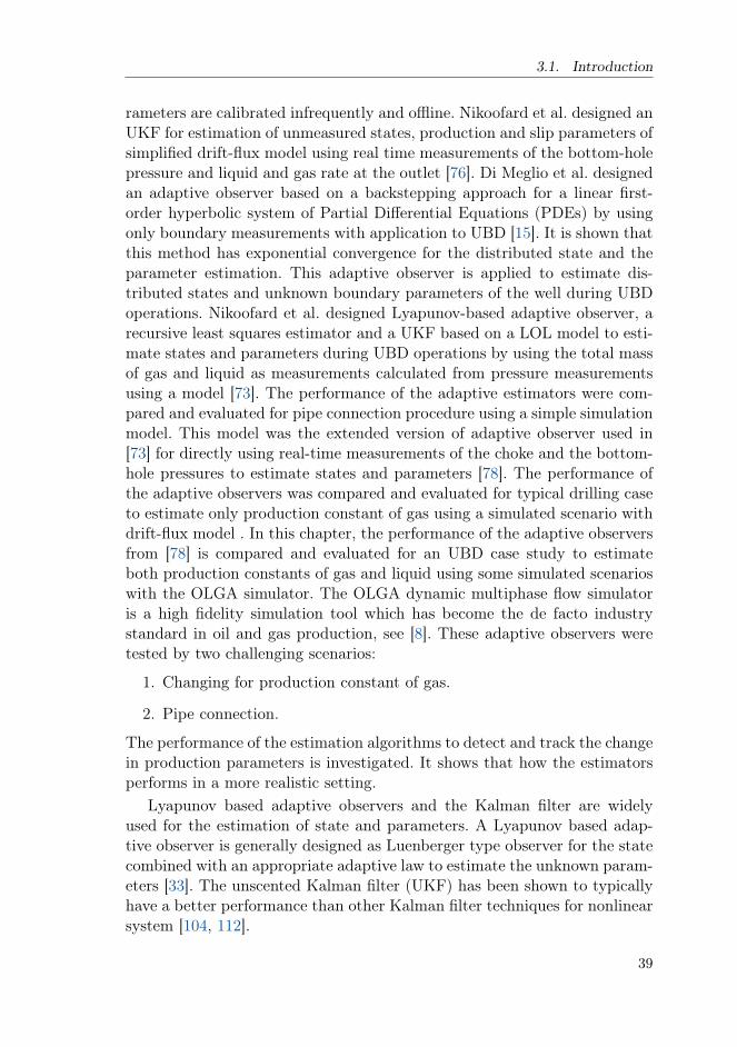
3.1. Introduction
rameters are calibrated infrequently and offline. Nikoofard et al. designed anUKF for estimation of unmeasured states, production and slip parameters ofsimplified drift-flux model using real time measurements of the bottom-holepressure and liquid and gas rate at the outlet [76]. Di Meglio et al. designedan adaptive observer based on a backstepping approach for a linear first-order hyperbolic system of Partial Differential Equations (PDEs) by usingonly boundary measurements with application to UBD [15]. It is shown thatthis method has exponential convergence for the distributed state and theparameter estimation. This adaptive observer is applied to estimate dis-tributed states and unknown boundary parameters of the well during UBDoperations. Nikoofard et al. designed Lyapunov-based adaptive observer, arecursive least squares estimator and a UKF based on a LOL model to esti-mate states and parameters during UBD operations by using the total massof gas and liquid as measurements calculated from pressure measurementsusing a model [73]. The performance of the adaptive estimators were com-pared and evaluated for pipe connection procedure using a simple simulationmodel. This model was the extended version of adaptive observer used in[73] for directly using real-time measurements of the choke and the bottom-hole pressures to estimate states and parameters [78]. The performance ofthe adaptive observers was compared and evaluated for typical drilling caseto estimate only production constant of gas using a simulated scenario withdrift-flux model . In this chapter, the performance of the adaptive observersfrom [78] is compared and evaluated for an UBD case study to estimateboth production constants of gas and liquid using some simulated scenarioswith the OLGA simulator. The OLGA dynamic multiphase flow simulatoris a high fidelity simulation tool which has become the de facto industrystandard in oil and gas production, see [8]. These adaptive observers weretested by two challenging scenarios:
1. Changing for production constant of gas.
2. Pipe connection.
The performance of the estimation algorithms to detect and track the changein production parameters is investigated. It shows that how the estimatorsperforms in a more realistic setting.
Lyapunov based adaptive observers and the Kalman filter are widelyused for the estimation of state and parameters. A Lyapunov based adap-tive observer is generally designed as Luenberger type observer for the statecombined with an appropriate adaptive law to estimate the unknown param-eters [33]. The unscented Kalman filter (UKF) has been shown to typicallyhave a better performance than other Kalman filter techniques for nonlinearsystem [104, 112].
39

3. Reservoir characterization in Under-balanced Drilling using Low-OrderLumped Model
The purpose of the chapter is to evaluate the LOL model for reservoircharacterization in UBD employing an adaptive observer that uses the bot-tom hole and choke pressure measurements from a simulated scenario withthe OLGA simulator. This chapter presents the design of a Lyapunov-basedadaptive observer and an UKF based on LOL model, and an UKF based ona simplified drift-flux model to estimate the states and geological propertiesof the reservoir (production parameters) during UBD operation. The perfor-mance of the adaptive observers based on LOL model is evaluated againstUKF based on a simplified drift-flux model by using measurements from theOLGA simulator. The adaptive observers are compared with each other interms of rate of convergence and accuracy. Robustness of the adaptive ob-servers is investigated in case of errors in the reservoir and well parametersof the models.
This chapter consists of the following sections: Section 3.2 describes thebasic concept of the UBD process. The modeling section presents a LOL andsimplified drift-flux model based on mass and momentum balances for UBDoperation and the reservoir model. Section 3.4 explains the Lyapunov-basedadaptive observer for and joint UKF methods for simultaneously estimatingthe states and model parameters from real-time measurements. At the endthe conclusion of the chapter is presented.
3.2 Under balanced drilling
In drilling operations, the drilling fluid is pumped down through the drillstring and the drill bit (see Figure 3.1). The annulus is sealed with a rotatingcontrol device (RCD), and the drilling fluid exits through a controlled chokevalve, allowing for faster and more precise control of the annular pressure.The drilling fluid carries cuttings from the drill bit to the surface.
In conventional (over-balanced) drilling, or managed pressure drilling(MPD), the pressure in the well is kept greater than pressure of reservoir toprevent influx from entering the well [29]. In UBD operations, on the otherhand the pressure of the well is kept below the pressure of the reservoir,allowing formation fluid flow into the well during the drilling operation.
Nitrogen unit, Rotating control devices (RCD), Chemical injection equip-ment, Surface separation equipment, choke and manifold system, geologicsampler, emergency shut-down system and Non-return valve (NRV) are themain surface equipments involved in normal UBD operations [102]. Thepump flow rate, choke valve and density of the drilling fluid (mud) are thevarious inputs used to adjust the pressure in the well-bore. The choke valveis the most common input used to regulate the pressure in the annulus dur-ing MPD and UBD operations. Furthermore, real time knowledge of states
40

3.3. Modeling
Figure 3.1: Schematic of an UBD system
and parameters of a dynamic model for the multi phase flow in the well isvery useful in controllers, fault detection systems and safety applications inthe well during petroleum exploration and production drilling. Some statesfor a dynamic model of multi phase flow in the well can not be measureddirectly or have a delay or low measurement frequency, and some parame-ters may be varied only during drilling. So, states and parameters for thedynamic model of multi phase flow in the well must be estimated.
3.3 Modeling
Due to the existence of multiphase flow (i.e. oil, gas, water, drilling mudand cuttings) in the system, the modeling of the system is challenging. Mul-tiphase flow can be modeled by a distributed model or a simplified LOL
41

3. Reservoir characterization in Under-balanced Drilling using Low-OrderLumped Model
model. A distributed model is capable of describing the gas-liquid behav-ior along the annulus in the well. The simplified LOL model is based onsome simplifying assumptions, and considers only the gas-liquid behavior atthe drill bit and the choke system. The LOL model used in this chapter isvery similar to the two-phase flow model found in [1, 81]. In the simplifieddrift-flux model and the LOL model, the drilling fluid, oil, water, and rockcuttings are lumped into the liquid phase. All models neglect the effects ofcutting transport as one of their assumption.
3.3.1 Simplified drift-flux model
There are two common methods for modeling distributed multiphase flowin UBD operations. The most general and detailed method is called a two-fluid model. This method uses four partial differential equations (PDE’s) forconservation of mass and momentum in each phase. The two-fluid model isdifficult to solve both analytically or numerically, because the source termsreflecting interphase drag are stiff and this can lead to significant problemsin the numerical computation [19]. Due to the complexity of the two-fluidmodel, the drift-flux model is derived by merging the momentum equationsof both phases (gas/liquid) into one equation. Therefore, difficult phase in-teraction terms cancel out, and the missing information in the mixture mo-mentum equation must be replaced by a slip equation which gives a relationbetween the flow velocities of the phases. The mechanistic models use dif-ferent relations between the phase slip velocities and pressure loss terms fordifferent flow patterns [46, 56]. These models need to predict flow patterns ateach time step. In this chapter, a simplified drift-flux model (DFM) is used.The simple DFM uses a specific empirical slip law, without flow-regime pre-dictions, but which allows for transition between single and two phase flows.The isothermal simple DFM formulation of the conservation of mass andmomentum balance are given by [3]
∂m
∂t+∂mvl∂x
= 0, (3.1)
∂n
∂t+∂nvg∂x
= 0, (3.2)
∂(mvl + nvg)
∂t+∂(P +mv2l + nv2g)
∂x= −(m+ n)g cos ∆θ − 2f(m+ n)vm|vm|
D.
(3.3)
where the mass variables are defined as follows
m = αlρl, n = αgρg
42

3.3. Modeling
where k = l, g denoting iquid and gas, respectively, ρk is the phase density,and αk is the volume fraction satisfying
αl + αg = 1. (3.4)
Further vk denotes the velocities, and P the pressure. All of these variablesare functions of time and space. We denote t ≥ 0 the time variable, andx ∈ [0, L] the space variable, corresponding to a curvilinear abscissa withx = 0 corresponding to the bottom hole and x = L to the outlet choke posi-tion. In the momentum equation (3.3), the term (m+n)g cos ∆θ representsthe gravitational source term, g is the gravitational constant and ∆θ is themean angle between gravity and the positive flow direction of the well, while−2f(m+n)vm|vm|
D accounts for frictional losses. The closure relations, bound-ary conditions and discretization schemes for this model can be found in[3].
3.3.2 LOL model
The so-called low-order lumped (LOL) model is perhaps the simplest methodfor modeling multiphase flow in UBD. A LOL model is suitable for conven-tional model-based control design methods and can be used for predictionand estimation in an observer and controller algorithms. The most importantsimplifying assumptions of the LOL model are listed as below:[81, 106]
• Ideal gas behavior
• Simplified choke model for gas, mud and liquid leaving the annulus
• No mass transfer between gas and liquid
• Isothermal condition and constant system temperature
• Constant liquid density with respect to pressure and temperature
• Uniform flow pattern along the whole drill string and annulus
The simplified LOL model equations for mass of gas and liquid in theannulus are derived from mass and momentum balances as follows [73]
mg = wg,d + wg,res(mg,ml)−mg
mg +mlwout(mg,ml) (3.5)
ml = wl,d + wl,res(mg,ml)−ml
mg +mlwout(mg,ml) (3.6)
wheremg andml are the total mass of gas and liquid, respectively. The liquidphase is assumed incompressible, and ρl is the liquid mass density. The gasphase is compressible and occupies the volume left free by the liquid phase.wg,d and wl,d are the mass flow rates of gas and liquid from the drill string,
43

3. Reservoir characterization in Under-balanced Drilling using Low-OrderLumped Model
and wg,res and wl,res are the mass flow rates of gas and liquid from thereservoir. The total mass outflow rate is
wout = KcZ
√mg +ml
Va
√pc − pc0 (3.7)
where Kc is the choke constant. Z is the control signal to the choke opening,taking its values on the interval (0, 1]. The total volume of the annulus isdenoted by Va, and pc0 is the constant downstream choke pressure (atmo-spheric). The choke pressure is denoted by pc, and derived from ideal gasequation
pc =RT
Mgas
mg
Va − mlρl
(3.8)
where R is the gas constant, T is the average temperature of the gas, andMgas is the molecular weight of the gas. The bottom-hole pressure is givenby the following equation
pbh = pc +(mg +ml)g cos(∆θ)
A+ ∆pf (3.9)
where A is the cross sectional area of the annulus,∆pf is the friction pressureloss in the well
∆pf = Kf (wg,d + wl,d)2 (3.10)
and Kf is the friction factor.
3.3.3 Reservoir flow
The mass flow from the reservoir into the well for each phase is modeled bya linear relation
wg,res =
{Kg(pres − pbh), if pres > pbh
0, otherwise.(3.11)
wl,res =
{Kl(pres − pbh), if pres > pbh
0, otherwise.(3.12)
where pres is the known pore pressure in the reservoir, and Kg and Kl
are the production constants of gas and liquid from the reservoir into thewell, respectively. Reservoir parameters could be evaluated by seismic dataand other geological data from core sample analysis. Still, local variations ofreservoir parameters such as the production constants of gas and liquid maybe revealed only during drilling. So, it is valuable to estimate the partialvariations of some of the reservoir parameters while drilling is performed([82]).
44
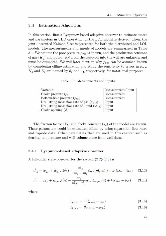
3.4. Estimation Algorithm
3.4 Estimation Algorithm
In this section, first a Lyapunov-based adaptive observer to estimate statesand parameters in UBD operation for the LOL model is derived. Then, thejoint unscented Kalman filter is presented for both the distributed and LOLmodels. The measurements and inputs of models are summarized in Table3.1. We assume the pore pressure pres is known, and the production constantof gas (Kg) and liquid (Kl) from the reservoir into the well are unknown andmust be estimated. We will later mention why pres can be assumed knownby considering offline estimation and study the sensitivity to errors in pres.Kg and Kl are named by θ1 and θ2, respectively, for notational purposes.
Table 3.1: Measurements and Inputs
Variables Measurement/InputChoke pressure (pc) MeasurementBottom-hole pressure (pbh) MeasurementDrill string mass flow rate of gas (wg,d) InputDrill string mass flow rate of liquid (wl,d) InputChoke opening (Z) Input
The friction factor (kf ) and choke constant (kc) of the model are known.These parameters could be estimated offline by using separation flow ratesand topside data. Other parameters that are used in this chapter such asdensity, temperature and well volume come from well data.
3.4.1 Lyapunov-based adaptive observer
A full-order state observer for the system (2.2)-(2.3) is
˙mg = wg,d + wg,res(θ1)−mg
mg + mlwout(mg, ml) + k1(pbh − pbh) (3.13)
˙ml = wl,d + wl,res(θ2)−ml
mg + mlwout(mg, ml) + k1(pbh − pbh) (3.14)
where
wg,res = θ1(pres − pbh) (3.15)
wl,res = θ2(pres − pbh) (3.16)
45

3. Reservoir characterization in Under-balanced Drilling using Low-OrderLumped Model
wout = KcZ
√mg + ml
Va
√pc − pc0 (3.17)
pbh = pc +(mg + ml)g cos(∆θ)
A+ ∆pf (3.18)
Note that the observer gains are chosen equal (k1 = k2) since it is basedon Lyapunov theorem. However, in practice it might be possible to choosedifferent gains based on tuning since Lyapunov theorem is conservative.k1A = l1 has to be chosen sufficiently large positive. mg and ml are estimatesof states mg and ml. Defining the state estimation errors e1 = mg− mg ande2 = ml − ml, θ1 and θ2 are estimates of parameters θ1 = Kg and θ2 = Kl.
˙θ1 = q1(pres − pbh)e1 (3.19)˙θ2 = q2(pres − pbh)e2 (3.20)
where the gains q1 and q2 are positive tuning parameters that specify trade-offs in the observer design. Choosing larger gains results in faster convergencebut large overshoot and undershoot in estimation, or sometimes instability.Choosing smaller gains results in slower convergence and small overshootand undershoot, or sometimes without any overshoot in estimation. Sincethe total mass of gas and liquid in the well could not be measured directly,they are computed by solving a series of nonlinear algebraic equations (3.8)-(3.9) using measurements of the choke and the bottom-hole pressures.
mcl =
1
1− pcMgas
RTρl
((pbh − pc −∆pf )A
g cos(∆θ)− pcMgasVa
RT
)(3.21)
mcg =
pcMgas(Va − mclρl
)
RT(3.22)
The adaptation laws (3.19)-(3.20) can be implemented by using e1 = mcg −
mg and e2 = mcl − ml. The error dynamics can be written as follows
e1 = (θ1 − θ1)(pres − pbh)− (mg
mg +mlwout −
mg
mg + mlwout)
− l1g cos(∆θ)(e1 + e2) (3.23)
e2 = (θ2 − θ2)(pres − pbh)− (ml
mg +mlwout −
ml
mg + mlwout)
− l1g cos(∆θ)(e1 + e2) (3.24)
Let θ1 = θ1 − θ1, θ2 = θ2 − θ2, and the Lyapunov function candidate foradaptive observer design be defined as
V (e, θ) =1
2(e21 + e22 + q−11 θ21 + q−12 θ22) (3.25)
46
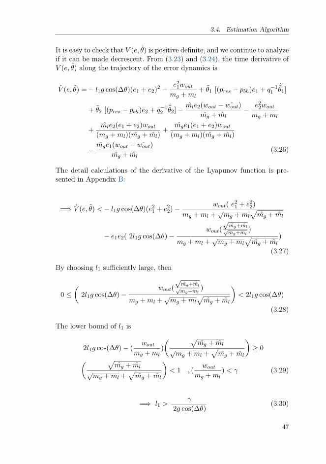
3.4. Estimation Algorithm
It is easy to check that V (e, θ) is positive definite, and we continue to analyzeif it can be made decrescent. From (3.23) and (3.24), the time derivative ofV (e, θ) along the trajectory of the error dynamics is
V (e, θ) =− l1g cos(∆θ)(e1 + e2)2 − e21wout
mg +ml+ θ1 [(pres − pbh)e1 + q−11
˙θ1]
+ θ2 [(pres − pbh)e2 + q−12˙θ2]−
mle2(wout − ˆwout)
mg + ml− e22woutmg +ml
+mle2(e1 + e2)wout
(mg +ml)(mg + ml)+
mge1(e1 + e2)wout(mg +ml)(mg + ml)
− mge1(wout − ˆwout)
mg + ml(3.26)
The detail calculations of the derivative of the Lyapunov function is pre-sented in Appendix B:
=⇒ V (e, θ) <− l1g cos(∆θ)(e21 + e22)−wout( e
21 + e22)
mg +ml +√mg +ml
√mg + ml
− e1e2( 2l1g cos(∆θ)−wout(
√mg+ml√mg+ml
)
mg +ml +√mg +ml
√mg + ml
)
(3.27)
By choosing l1 sufficiently large, then
0 ≤(
2l1g cos(∆θ)−wout(
√mg+ml√mg+ml
)
mg +ml +√mg +ml
√mg + ml
)< 2l1g cos(∆θ)
(3.28)
The lower bound of l1 is
2l1g cos(∆θ)− (wout
mg +ml)
( √mg + ml√
mg +ml +√mg + ml
)≥ 0( √
mg + ml√mg +ml +
√mg + ml
)< 1 , (
woutmg +ml
) < γ (3.29)
=⇒ l1 >γ
2g cos(∆θ)(3.30)
47

3. Reservoir characterization in Under-balanced Drilling using Low-OrderLumped Model
In real drilling problem we usually have (γ � 1), therefore the lower boundof l1 is small, and this gives
V (e, θ) < −l1g cos(∆θ)(e21 + e22) + 2l1g cos(∆θ)|e1||e2|
− wout( e21 + e22)
mg +ml +√mg +ml
√mg + ml
(3.31)
By using Young’s inequality 2|e1||e2| ≤ e21 + e22,
V (e, θ) < − wout( e21 + e22)
mg +ml +√mg +ml
√mg + ml
≤ 0 (3.32)
which implies that all signals e1, e2, θ1, θ2 are bounded. From (3.23),(3.24)and e1, e2, θ1, θ2 ∈ L∞, e1, e2 are bounded. It follows by using Barbalat’slemma that e1, e2 converge to zero. Based on equation (3.19)-(3.20), theadaptation laws can be written as follows:
˙θ =
[˙θ1˙θ2
]=
[q1 00 q2
] [pres − pbh 0
0 pres − pbh
] [e1e2
]Γ =
[q1 00 q2
], φ = (pres − pbh)I, ζ =
[e1e2
]=⇒ ˙
θ = Γφζ (3.33)
Based on the persistency excitation theorem,limt→∞ θ = θ∗ if and only ifthere exists some α, T > 0 such that, for any t > 0 , the following inequalityis satisfied ([33]):∫ t+T
tφ(τ)φT (τ) dτ ≥ αI > 0, ∀t ≥ t0 (3.34)
So,∫ t+T
tφ(τ)φT (τ) dτ =
∫ t+T
t(pres(τ)− pbh(τ))2I dτ ≥ αI > 0, ∀t ≥ t0
(3.35)
Thus according to theorem 4.9 in [40], the adaptive observer system is glob-ally asymptotically stable if the persistency excitation condition is satisfied.There must be flow from the reservoir to satisfy persistence exciting condi-tion.
3.4.2 Joint Unscented Kalman Filter
The Kalman filter using linearization to estimate both the state and param-eter vectors of the system is usually known as an augmented Kalman filter.
48

3.5. Simulation Results
The UKF technique has been developed to work with non-linear systemswithout using an explicit linearization of the model ([36, 37]). The UKFestimates the mean and covariance matrix of the estimation error with aminimal set of sample points (called sigma points) around the mean by us-ing a deterministic sampling approach known as the unscented transform.The nonlinear model is applied to propagate uncertainty of sigma pointsinstead of using a linearization of the model. So, this method does not needto calculate the explicit Jacobian or Hessian. More details can be found in([36, 104]).
The augmented state vector is defined by xa = [X, θ] where X is the stateof the model. The discrete state-space equations for the the augmented statevector at time instant k is written as:[
Xk
θk
]=
[f(Xk−1, θk−1)
θk−1
]+ qk = fa(Xk−1, θk−1) + qk (3.36)
where qk ∼ N(0, Qk) is the zero mean Gaussian process noise (model error).Here, we apply the UKF to both the LOL and DFM. When using the DFM,the number of states that must be estimated by the joint UKF is equalto three times of the number of spatial discretization cells in the drift-fluxmodel. The discrete measurements of the system can be modeled as follows:
yk = h(Xk) + rk (3.37)
h(Xk) = [pc, pbh]T (3.38)
where rk ∼ N(0, Rk) is the zero mean Gaussian measurement noise.
3.5 Simulation Results
The parameter values for the simulated well and reservoir are summarizedin Table 3.2, and used in the OLGA simulator. The measurements havebeen synthetically generated by using the OLGA dynamic multiphase flowsimulator. The OLGA simulator uses the same model for the mass flow fromthe reservoir into the well as in equations (3.11)-(3.12).
A discretization of the time and space variables is required for usingnumerical methods. The PDE of the drift-flux model are discretized by usinga finite volumes method for the joint UKF based on DFM. where 6 cellswere used for the spatial discretization. A measurement sampling period of10 seconds were used and the model was run with time steps of 10 seconds.The parameter values for the nonlinear adaptive observer and UKF for bothmodels are summarized in Table 3.3.
The initial values for the estimated and real parameters are as follows:
Kg = 0.05, Kl = 0.1, Kg = 0.07, Kl = 0.13
49

3. Reservoir characterization in Under-balanced Drilling using Low-OrderLumped Model
Table 3.2: Parameter Values for Well and Reservoir
Name DFM UnitReservoir pressure (pres) 279 barCollapse pressure (pcoll) 155 barWell total length (Ltot) 2530 mDrill string outer diameter (Dd) 0.1206 mAnnulus inner diameter (Da) 0.1524 mLiquid flow rate (wl,d) 13.33 kg/sGas flow rate (wg,d) 0 kg/sLiquid density (ρL) 1000 kg/m3
Production constant of liquid (KL) 0.1 kg/s/barGas average temperature (T ) 285.15 KAverage angle (∆θ) 0 radChoke constant (Kc) 0.0057 m2
Table 3.3: Parameter Values for Model and Estimators
Parameter Value Parameter Valueq1 2.5× 10⁻¹³ k1 4× 10⁻⁹
q2 5× 10⁻¹⁴ L 4κLOL 0 κDFM 0αLOL 0.00001 αDFM 0.00001βLOL 2 βDFM 2
The case study that is used in this chapter considers UBD operation of avertical well drilled into an oil and gas reservoir. Two scenarios are simulated.In first scenario, first drilling in a steady-state condition is initiated with thechoke opening of 12 %. After 1 hour, there is a linear decrease in the chokeopening from 12 % to 8 % for 1 hour. After 4 hours, there is a linear increasein the choke opening from 8 % to 12 % for 1 hour. After 7 hours, there isa linear and sharp increase in the production constant of gas from 0.05kg/s/bar to 0.07 kg/s/bar (change of reservoir height). Choke opening inthis simulation is illustrated in Figure 3.2. The parameter covariance matrixof UKF used for both models and scenarios is
Q = diag[8 ∗ 10−9, 2 ∗ 10−8]
Choosing the process noise covariance matrix in the UKF (Qk) specify trade-offs in the UKF design. Choosing larger process noise in the UKF (Qk)leads to faster track of data and convergence but typically more uncertaintyin the estimation. Choosing smaller process noise in the UKF (Qk) leadsto slower track of data and convergence but typically less uncertainty in
50
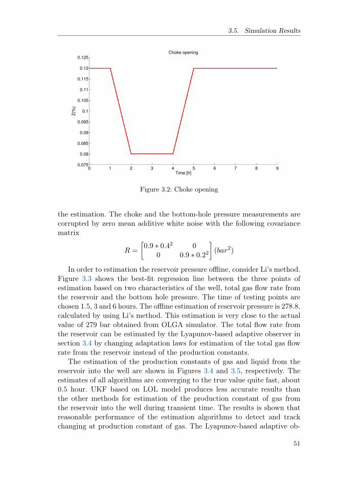
3.5. Simulation Results
0 1 2 3 4 5 6 7 8 90.075
0.08
0.085
0.09
0.095
0.1
0.105
0.11
0.115
0.12
0.125
Z(%
)
Choke opening
Time [h]
Figure 3.2: Choke opening
the estimation. The choke and the bottom-hole pressure measurements arecorrupted by zero mean additive white noise with the following covariancematrix
R =
[0.9 ∗ 0.42 0
0 0.9 ∗ 0.22
](bar2)
In order to estimation the reservoir pressure offline, consider Li’s method.Figure 3.3 shows the best-fit regression line between the three points ofestimation based on two characteristics of the well, total gas flow rate fromthe reservoir and the bottom hole pressure. The time of testing points arechosen 1.5, 3 and 6 hours. The offline estimation of reservoir pressure is 278.8,calculated by using Li’s method. This estimation is very close to the actualvalue of 279 bar obtained from OLGA simulator. The total flow rate fromthe reservoir can be estimated by the Lyapunov-based adaptive observer insection 3.4 by changing adaptation laws for estimation of the total gas flowrate from the reservoir instead of the production constants.
The estimation of the production constants of gas and liquid from thereservoir into the well are shown in Figures 3.4 and 3.5, respectively. Theestimates of all algorithms are converging to the true value quite fast, about0.5 hour. UKF based on LOL model produces less accurate results thanthe other methods for estimation of the production constant of gas fromthe reservoir into the well during transient time. The results is shown thatreasonable performance of the estimation algorithms to detect and trackchanging at production constant of gas. The Lyapunov-based adaptive ob-
51
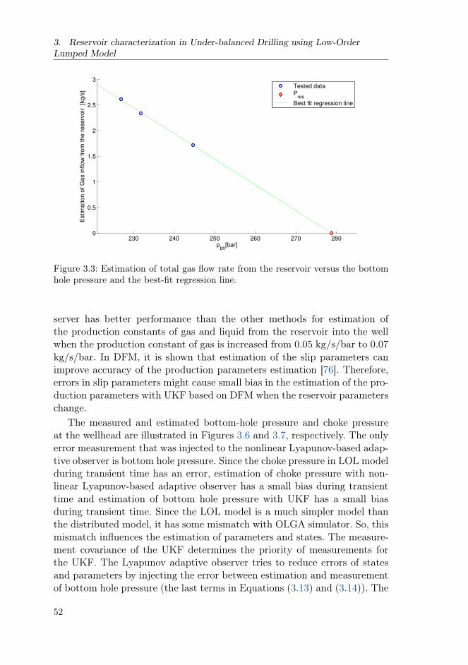
3. Reservoir characterization in Under-balanced Drilling using Low-OrderLumped Model
230 240 250 260 270 2800
0.5
1
1.5
2
2.5
3
pbh
[bar]
Estim
atio
n o
f G
as in
flo
w f
rom
th
e r
ese
rvo
ir
[kg
/s]
Tested data P
res
Best fit regression line
Figure 3.3: Estimation of total gas flow rate from the reservoir versus the bottomhole pressure and the best-fit regression line.
server has better performance than the other methods for estimation ofthe production constants of gas and liquid from the reservoir into the wellwhen the production constant of gas is increased from 0.05 kg/s/bar to 0.07kg/s/bar. In DFM, it is shown that estimation of the slip parameters canimprove accuracy of the production parameters estimation [76]. Therefore,errors in slip parameters might cause small bias in the estimation of the pro-duction parameters with UKF based on DFM when the reservoir parameterschange.
The measured and estimated bottom-hole pressure and choke pressureat the wellhead are illustrated in Figures 3.6 and 3.7, respectively. The onlyerror measurement that was injected to the nonlinear Lyapunov-based adap-tive observer is bottom hole pressure. Since the choke pressure in LOL modelduring transient time has an error, estimation of choke pressure with non-linear Lyapunov-based adaptive observer has a small bias during transienttime and estimation of bottom hole pressure with UKF has a small biasduring transient time. Since the LOL model is a much simpler model thanthe distributed model, it has some mismatch with OLGA simulator. So, thismismatch influences the estimation of parameters and states. The measure-ment covariance of the UKF determines the priority of measurements forthe UKF. The Lyapunov adaptive observer tries to reduce errors of statesand parameters by injecting the error between estimation and measurementof bottom hole pressure (the last terms in Equations (3.13) and (3.14)). The
52

3.5. Simulation Results
0 1 2 3 4 5 6 7 8 90.04
0.045
0.05
0.055
0.06
0.065
0.07
0.075
0.08
Kg[k
g/s
/ba
r]
Trend
Time [h]
Lyapunov based adaptive observer
OLGA
UKF based on LOL model
UKF based on DFM
Figure 3.4: Actual value and estimated production constant of gas
0 1 2 3 4 5 6 7 8 90.08
0.09
0.1
0.11
0.12
0.13
0.14
0.15
Kl[k
g/s
/ba
r]
Trend
Time [h]
Lyapunov based adaptive observerOLGA
UKF based on LOL modelUKF based on DFM
Figure 3.5: Actual value and estimated production constant of liquid
53

3. Reservoir characterization in Under-balanced Drilling using Low-OrderLumped Model
bottom hole pressure and the choke pressure are correlated with each otherwith the mass and momentum balances. So, the error between estimationand measurement of choke pressure is indirectly affected by the Lyapunovadaptive observer. But, the error between estimation and measurement ofbottom hole pressure is affected directly by the Lyapunov adaptive observer.Simulation time of adaptive observers based on LOL model executes at least100 times faster than joint UKF based on DFM.
0 1 2 3 4 5 6 7 8 9220
225
230
235
240
245
250Trend
pbh[b
ar]
Time [h]
Measurements from OLGALyapunov based adaptive observerUKF based on LOL modelUKF based on DFM
Figure 3.6: Measured and estimated bottom-hole pressure
In this chapter, performance of these adaptive observers is evaluatedthrough the root mean square error (RMSE) metric for the parameters Kg
and Kl . The RMSE metric for Lyapunov-based adaptive observer and UKFfor both models during the whole estimation period and after initial transient(t ≥ 0.5hour) are summarized in Table 3.4.
According to the RMSE metric Table 3.4, the Lyapunov-based adaptiveobserver has better performance than the other methods for estimation ofthe production constants of gas and liquid from the reservoir into the well.
Robustness of the adaptive observers is tested in case of errors in thereservoir and well parameters of the models. This test is performed in caseof errors in the reservoir pore pressure and liquid density. The RMSE metricfor the adaptive observers in two case of 1% error on the reservoir porepressure and 10% error on the liquid density are summarized in Table 3.5and 3.6, respectively.
54

3.5. Simulation Results
0 1 2 3 4 5 6 7 8 90
10
20
30
40
50
60
Trend
pc[b
ar]
Time [h]
Measurements from OLGALyapunov based adaptive observer
UKF based on LOL modelUKF based on DFM
Figure 3.7: Measured and estimated choke pressure
Table 3.4: RMSE metric
Method Whole estimation period After initial transientKg Kl Kg Kl
Lyapunov method 1.4× 10⁻³ 4.0× 10⁻³ 1.1× 10⁻³ 3.3× 10⁻³
UKF based on LOL model 3.6× 10⁻³ 5.0× 10⁻³ 3.4× 10⁻³ 4.5× 10⁻³
UKF based on DFM 3.5× 10⁻³ 6.8× 10⁻³ 3.3× 10⁻³ 5.2× 10⁻³
Table 3.5: RMSE metric in case of error in the reservoir pressure value
Method Kg Kl pres true pres modelLyapunov method 4× 10⁻³ 8× 10⁻³ 279 282UKF based on LOL model 5.7× 10⁻³ 9× 10⁻³ 279 282UKF based on DFM 5.9× 10⁻³ 9.9× 10⁻³ 279 282
Table 3.6: RMSE metric in case of error in the liquid density value
Method Kg Kl ρL true ρL modelLyapunov method 2.6× 10⁻³ 5.2× 10⁻³ 1000 1100UKF based on LOL model 3.4× 10⁻³ 6.4× 10⁻³ 1000 1100UKF based on DFM 3.6× 10⁻³ 6.9× 10⁻³ 1000 1100
55

3. Reservoir characterization in Under-balanced Drilling using Low-OrderLumped Model
Since the reservoir pore pressure has a direct effect on the mass flowrates from the reservoir into the well, small inaccuracies in the reservoir porepressure have a significant effect on the estimation of production constants.Therefor these methods are very sensitive to errors in the reservoir porepressure value. Adaptive observers based on LOL model are more sensitiveto errors in the liquid density value than UKF based on DFM.
The second scenario in this case study is as follows, first the drilling in asteady-state condition is initiated with the choke opening of 10 %, then att = 1 hour and 35 min the main pump is shut off to perform a connectionprocedure, and the choke is closed to 6 %. The rotation of the drill stringand the circulation of fluids are stopped for 15 mins. Next after making thefirst pipe connection at t = 1 hour and 50 min the main pump and rotationof the drill string are restarted. After 1 hour and 45 min (i.e. 3 hour and 35min), the choke is closed to 5 %, and the second pipe connection procedureis started, and is completed after 15 mins. Then the choke is opened to 10 %at t= 3 hours and 50 min. The measured bottom-hole pressure (pbh), chokepressure (pc), choke opening (Z), and mass flow rate of liquid from the drillstring (wl,d) is illustrated in Figure 3.8.
0 0.5 1 1.5 2 2.5 3 3.5 4 4.5 5 5.5200
220
240
260Trend
Time [h]
pbh[b
ar]
0 0.5 1 1.5 2 2.5 3 3.5 4 4.5 5 5.50
5
10
15
wl,d(k
g/s
)
0 0.5 1 1.5 2 2.5 3 3.5 4 4.5 5 5.540
60
80
100
120
Time [h]
pc[b
ar]
0 0.5 1 1.5 2 2.5 3 3.5 4 4.5 5 5.50.04
0.06
0.08
0.1
0.12
Choke o
penin
g (
%)
Figure 3.8: Measured bottom-hole pressure, choke pressure, choke opening, andmass flow rate of liquid from the drill string for pipe connection scenario
The parameter values for the nonlinear adaptive observer and UKF forboth models for pipe connection scenario are the same as previous scenario.
56

3.5. Simulation Results
The initial values for the estimated and real parameters are as follows:
Kg = 0.07, Kl = 0.1, Kg = 0.091, Kl = 0.13
The estimation of the production constants of gas and liquid from the reser-voir into the well are shown in Figures 3.9 and 3.10, respectively. Theseparameters are identified correctly by all estimators. In estimation of pro-duction constant of liquid from the reservoir into the well, Lyapunov-basedadaptive observer has better performance than the other methods. Since themodel is significantly less accurate during the pipe connection, we need toprevent that the PI estimates drift away. Hence, the gains value (q1 and q2)for Lyapunov-based adaptive observer and the parameter covariance of UKFfor both models are 1000 times smaller than the nominal value during thepipe connection. For the same reason, the measurement covariance of UKFfor both models are 1000 times larger than the nominal value during thepipe connection.
0 0.5 1 1.5 2 2.5 3 3.5 4 4.5 5 5.50.065
0.07
0.075
0.08
0.085
0.09
0.095
Kg[k
g/s
/bar]
Trend
Time [h]
Lyapunov based adaptive observer
OLGA
UKF based on LOL model
UKF based on DFM
Figure 3.9: Actual value and estimated production constant of gas for pipe connec-tion scenario
The measured and estimated bottom-hole pressure and choke pressureat the wellhead for pipe connection scenario are illustrated in Figures 3.11and 3.12, respectively. This results show that adaptive observers have errorin estimation of the bottom hole and choke pressure during pipe connectionbecause the model is less accurate during pipe connection. Since the bottom
57

3. Reservoir characterization in Under-balanced Drilling using Low-OrderLumped Model
0 0.5 1 1.5 2 2.5 3 3.5 4 4.5 5 5.50.095
0.1
0.105
0.11
0.115
0.12
0.125
0.13
Kl[k
g/s
/ba
r]Trend
Time [h]
Lyapunov based adaptive observerOLGA
UKF based on LOL modelUKF based on DFM
Figure 3.10: Actual value and estimated production constant of liquid for pipeconnection scenario
hole and choke pressure are measured, errors of the bottom hole and chokepressure are not the main concern in this situation. Based on Nygaard et al.studied that some parameters of the model such as friction factor varies dur-ing pipe connection [85]. Since we assumed these parameters are constant,it introduces some errors to the model during pipe connection.
The RMSE metric of the parameters Kg and Kl for Lyapunov-basedadaptive observer and UKF for both models after initial transient (t ≥0.5hour) are summarized in Table 3.7.
Table 3.7: RMSE metric for estimate of Kg and Kl for pipe connection scenario
Method Kg(after t ≥ 0.5h) Kl(after t ≥ 0.5h)Lyapunov-based adaptive observer 0.7× 10⁻³ 1.6× 10⁻³
UKF based on LOL model 0.7× 10⁻³ 3.7× 10⁻³
UKF based on DFM 1.3× 10⁻³ 3.7× 10⁻³
According to the RMSE metric Table 3.7, the Lyapunov-based adaptiveobserver has better performance than the other methods for estimation ofthe production constants of gas and liquid from the reservoir into the wellin pipe connection scenario.
58
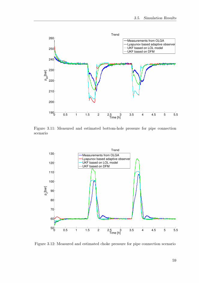
3.5. Simulation Results
0 0.5 1 1.5 2 2.5 3 3.5 4 4.5 5 5.5190
200
210
220
230
240
250
260Trend
pbh[b
ar]
Time [h]
Measurements from OLGALyapunov based adaptive observerUKF based on LOL modelUKF based on DFM
Figure 3.11: Measured and estimated bottom-hole pressure for pipe connectionscenario
0 0.5 1 1.5 2 2.5 3 3.5 4 4.5 5 5.550
60
70
80
90
100
110
120
130Trend
pc[b
ar]
Time [h]
Measurements from OLGALyapunov based adaptive observer
UKF based on LOL modelUKF based on DFM
Figure 3.12: Measured and estimated choke pressure for pipe connection scenario
59
3. Reservoir characterization in Under-balanced Drilling using Low-OrderLumped Model
3.6 Conclusion
A simplified DFM and a LOL model describing a multiphase (gas-liquid)flow in the well during UBD has been used. This chapter presents Lyapunov-based adaptive observer and joint UKF based on LOL model for reservoircharacterization during UBD operations. Furthermore, it describes a jointUKF to estimate parameters and states for the simplified DFM by usingreal-time measurements of the choke and the bottom-hole pressures fromOLGA simulator. The results show that all estimators are capable of iden-tifying the production constants of gas and liquid from the reservoir intothe well. All adaptive observers have a quite fast convergence rate, about0.5 hour. Simulation results demonstrated reasonable performance of theestimation algorithms to detect and track a changing gas production coeffi-cient using a simulated scenario with OLGA. The nonlinear Lyapunov-basedadaptive observer has better accuracy than the other methods for estima-tion of the production constants of gas and liquid from the reservoir into thewell. Adaptive observers based on the LOL model are computationally sim-pler than joint UKF based on DFM. However, adaptive observers based onLOL model are more sensitive to errors in the reservoir and well parametersof the model than joint UKF based on DFM.
60
CHAPTER4State and parameter estimation of a
Drift-Flux Model for Under-BalancedDrilling operations
4.1 Introduction
There have been an increasing research focus on automation of drilling forexploration and production of hydrocarbons in the recent years. Modeling forestimation, and model-based control techniques have been studied in a widerange of drilling and production scenarios. In Managed Pressure Drilling(MPD), a back-pressure pump in conjunction with a back pressure choke isused to control the pressure in the well, posing new control and estimationchallenges. In a typical scenario, the control goal is to keep the pressureof the well (pwell(t, x)) greater than pressure of the reservoir (pres(t, x)) toprevent influx from entering the well, but lower than the fracture pressure(pfrac(t, x)) to avoid the loss of drilling fluids to the reservoir [24]
pres(t, x) < pwell(t, x) < pfrac(t, x) (4.1)
at all times t and along the well profile x ∈ [0, L].In an alternative approach, known as Under-Balanced Drilling (UBD),
the pressure in the well is kept greater than the collapse pressure of the wellbut lower than the pressure of the reservoir [9]
pcoll(t, x) < pwell(t, x) < pres(t, x) (4.2)
In this case, due to the pressure drawdown (meaning the positive differenceof the reservoir pressure and well pressure) inflow fluid, in many cases gas,is produced continuously from the reservoir. The rate of reservoir inflow istypically approximated mathematically by a so-called Production Index (PI)
61

4. State and parameter estimation of a Drift-Flux Model for Under-BalancedDrilling operations
parameter
qinflux = PI.max(pres − pbh, 0). (4.3)
Especially for under-balanced wells producing gas, the magnitude of the PIhas a significant impact on the dynamics of the UBD and thus also on thecontrol problem. Hence, accurate estimates of the PI and reservoir pressureare important for an UBD operation.
Modeling of UBD operations and MPD scenarios handling influx requiresa multiphase model. A popular model in the literature is the Drift-FluxModel (DFM) [19, 45, 56]. The drift flux model is a set of first order non-linear hyperbolic partial differential equations (PDE). In case of two-phaseflow, it consists of three governing equations. The Low-Order Lumped (LOL)models are simpler methods that can be used. However, these models areonly able to capture the major effects in the well and for the general purposeit produces less accurate results [73, 81, 106].Due to the complexity of the multi-phase flow dynamics of a UBD well cou-pled with a reservoir, the modeling, estimation and model based control ofUBD operations is still considered an emerging and challenging topic withindrilling automation. Nygaard et al.[82] compared and evaluated the perfor-mance of the extended Kalman filter, the ensemble Kalman filter and theunscented Kalman filter based on a low order model to estimate the statesand the PI in UBD operation. In Nygaard et al. [85], a finite horizon non-linear model predictive control in combination with an unscented Kalmanfilter was designed for controlling the bottom-hole pressure based on a loworder model developed in [81] for pipe connection scenario. The unscentedKalman filter was used to estimate the states, and the friction and chokecoefficients. Nikoofard et al.[73] designed a Lyapunov-based adaptive ob-server, a recursive least squares estimation and a joint unscented Kalmanfilter based on a low-order lumped model to estimate states and parame-ters during UBD operations. This model was the extended version of adap-tive observer used in [73] for directly using real-time measurements of thechoke and the bottom-hole pressures to estimate states and parameters [78].The performance of the adaptive observers was compared and evaluatedfor typical drilling case to estimate only production constant of gas usinga simulated scenario with a drift-flux model. A Nonlinear Moving HorizonObserver based on a low-order lumped model was designed for estimatingthe total mass of gas and liquid in the annulus and geological propertiesof the reservoir during UBD operation in [74]. The problem of parameterestimation in multiphase flows is often referred to as ’soft-sensing’ in thecontext of production, see[11, 28, 57, 58, 108].
Lorentzen et al. designed an ensemble Kalman filter based on the drift-
62

4.1. Introduction
flux model to tune the uncertain parameters of a two-phase flow model inthe UBD operation [56]. Vefring et al.[110, 111] compared and evaluatedthe performance of the ensemble Kalman filter and an off-line nonlinearleast squares technique utilizing the Levenberg-Marquardt optimization al-gorithm to estimate reservoir pore pressure and reservoir permeability duringUBD while performing an excitation of the bottom-hole pressure. The resultshows that excitation of the bottom-hole pressure might improve the esti-mation of the reservoir pore pressure and reservoir permeability [110, 111].Aarsnes et al.[2] used a drift-flux model and an Extended Kalman Filter toestimate the states and PI online, and suggested a scheme combining thiswith off-line calibration using the algorithm in [110]. The provided analysisalso suggests how such a scheme fits into the UBD operating envelope asproposed by [26], and explored in [3]. Di Meglio et al. designed an adaptiveobserver based on a backstepping approach for a linear first-order hyperbolicsystem of Partial Differential Equations (PDEs) by using only boundarymeasurements with application to UBD [15]. It is shown that this methodhas exponential convergence for the distributed state and the parameter es-timation. This adaptive observer is applied to estimate distributed statesand unknown boundary parameters of the well during UBD operations. GaoLi et al. presented an algorithm for characterizing reservoir pore pressureand reservoir permeability during UBD of horizontal wells [52]. Since thetotal flow rate from the reservoir has a negative linear correlation with thebottom hole pressure, reservoir pore pressure can be identified by the cross-ing of the horizontal axis and the best-fit regression line between the totalflow rate from the reservoir and the bottom hole pressure while performingan excitation of the bottom-hole pressure by changing the choke valve open-ing or pump rates. The unscented Kalman filter (UKF) has been shown totypically have a better performance than other Kalman filter techniques fornonlinear system ([104, 112]). Nikoofard et al. used an UKF with the drift-flux model for the first time [76]. They designed an UKF for estimation ofunmeasured states, production and slip parameters of simplified drift-fluxmodel using real time measurements of the bottom-hole pressure and liquidand gas rate at the outlet [76]. This chapter is an extended version of workpublished in [76] which presents the design of a UKF based on a simplifieddrift-flux model to estimate the states, geological properties of the reservoirand slip parameters during UBD operation. In this work, both productionconstants of gas and liquid and unmeasured states are estimated by usingonly measurements of the choke and the bottom-hole pressures during UBDoperation for pipe connection procedure. The performance of UKF is eval-uated against EKF by using measurements from OLGA simulator and theconsequences of not estimating slip parameters are discussed.These adaptive
63

4. State and parameter estimation of a Drift-Flux Model for Under-BalancedDrilling operations
observers were tested by two challenging scenarios:1. Changing for production constant of gas.
2. Pipe connection.The performance of the estimation algorithms to detect and track the changein production parameters is investigated. Robustness of the UKF and EKFfor the pipe connection scenario is studied in case of uncertainties and errorsin the reservoir and well parameters of the model. This chapter is organizedas follows: Section 4.2 presents the simplified drift-flux model based on massand momentum balances for UBD operation. Section 4.3 explain UKF andEKF for simultaneously estimating the states and parameters of a simplifieddrift-flux model from OLGA simulator measurements. In the section 4.4, thesimulation results are provided for state and parameter estimation. At theend the conclusion of the chapter are presented.
4.2 The drift flux model
The model employed is the same as the one used in [3]. It expresses themass conservation law for the gas and the liquid separately, and a combinedmomentum equation. The mud, oil and water are lumped into one singleliquid phase. In developing the model, the following mass variables are used
m = αLρL, n = αGρG
where for k = L,G denoting liquid or gas, ρk is the phase density, and αk isthe volume fraction satisfying
αL + αG = 1. (4.4)
Further vk denotes the velocities, and P the pressure. All of these variablesare functions of time and space. We denote t ≥ 0 the time variable, andx ∈ [0, L] the space variable, corresponding to a curvilinear abscissa with x= 0 corresponding to the bottom hole and x = L to the outlet choke position(see Fig. 4.1). The isothermal equations are as follows,
∂m
∂t+∂mvL∂x
= 0, (4.5)
∂n
∂t+∂nvG∂x
= 0, (4.6)
∂(mvL + nvG)
∂t+∂(P +mv2L + nv2G)
∂x
= −(m+ n)g cos ∆θ − 2f(m+ n)vm|vm|D
. (4.7)
64

4.2. The drift flux model
Figure 4.1: Drilling process schematic for UBD.
In the momentum equation (4.7), the term (m + n)g cos ∆θ represents thegravitational source term„ g is the gravitational constant and ∆θ is themean angle between gravity and the positive flow direction of the well, while−−2f(m+n)vm|vm|
D accounts for frictional losses. The mixtures velocity is givenas
vm = αGvG + αLvL. (4.8)
Along with these distributed equations, algebraic relations are needed todescribe the system.
65

4. State and parameter estimation of a Drift-Flux Model for Under-BalancedDrilling operations
4.2.1 Closure Relations
Both the liquid and gas phase are assumed compressible. This is requiredfor the model to handle the transition from two-phase to single-phase flow.The densities are thus given as functions of the pressure as follows
ρG =P
c2G, ρL = ρL,0 +
P
c2L, (4.9)
where ck is the velocity of sound and ρL,0 is the reference density of theliquid phase given at vacuum. Notice that the velocity of sound in the gasphase cG depends on the temperature as suggested by the ideal gas law. Thetemperature profile is assumed to be known.Combining (4.9) with (4.4) we obtain the following relations for findingvolume fractions from the mass variables:
αG =1
2−
c2Gc2Ln+m+
√∆
2ρL,0, (4.10)
∆ =(ρL,0 −
c2Gc2Ln−m
)2+ 4
c2Gc2LnρL,0 (4.11)
Then the pressure can be found using a modified expression to ensure pres-sure is define when the gas vanishes
P =
{(m
1−αG− ρL,0
)c2L, if αG ≤ α∗G
nαGc2G, otherwise.
(4.12)
α∗G is typically chosen as 0.5. Because the momentum equation (4.7) waswritten for the gas-liquid mixture, a so-called slip law is needed to empiri-cally relate the velocities of gas and liquid. To handle the transition betweensingle and two-phase flow, a relation with state-dependent parameters isneeded ([18, 103]).
vG = (K − (K − 1)αG)vm + αLS (4.13)
where K ≥ 1 and S ≥ 0 are constant parameters.
4.2.2 Boundary Conditions
Boundary conditions are given by the mass-rates of gas and liquid injectedfrom the drilling rig and flowing in from the reservoir. Denoting the crosssectional flow area by A, the boundary fluxes are given as:
mvL|x=0 =1
A
(WL,res(t) +WL,inj(t)
), (4.14)
nvG|x=0 =1
A
(WG,res(t) +WG,inj(t)
). (4.15)
66

4.2. The drift flux model
The injection mass-rates of gas and liquid, WG,inj ,WL,inj , are specified bythe driller and can, within some constraints, be considered as manipulatedvariables. The inflow from the reservoir is dependent on the pressure onthe left boundary, for which, within the operational range of a typical UBDoperation, an affine approximation should suffice, i.e.
WL,res = kL max(Pres−P (0), 0) (4.16)WG,res = kG max(Pres−P (0), 0) (4.17)
Here Pres is the reservoir pore pressure and kG, kL are the production index(PI) of the gas and liquid respectively.
The topside boundary condition is given by a choke equation relatingtopside pressure to mass flow rates
mvL√ρL
+nvGY√ρG
∣∣∣x=L
=Cv(Z)
A
√max (P (L, t)− Ps, 0), (4.18)
where Cv is the choke opening given by the manipulated variable Z. Y ∈[0, 1] is a gas expansion factor for the gas flow and Ps is the separatorpressure, i.e. the pressure downstream the choke.
4.2.3 Numerical Implementation
The drift flux model described above was implemented using a fully implicitBackwards Time-Central Space (BTCS) finite differences numerical schemewith an explicitly derived Jacobian as described in [3].
Define the state vector to be made up of the conservative mass variablesm,n and combined momentum I = mvL + nvL, u =
[m n I
]T . For eachof the states we use the following definition for finite differences,
mki = m(k∆t, i∆x), etc.
where i = 0, 1, . . . , N and k = 0, 1, . . . . We arrange the terms into a vector
uk =[mk
1,mk2, . . . ,m
kN , n
k1, . . . , n
kN , I
k1 , . . . , I
kN
].
Consequently, propagating the states in time from uk to uk+1 equates tosolving a set of nonlinear equations that are implicit in uk+1, which wedenote as
F (uk+1,uk) = 0, F : R3N × R3N → R3N . (4.19)
These are solved using Newton steps which require the inverse of the Ja-cobian of F w.r.t. Xk+1 denoted FXk+1
. We note that the existence of thisinverse is guaranteed by the 1/∆t terms making up the diagonal of FXk+1
.
67

4. State and parameter estimation of a Drift-Flux Model for Under-BalancedDrilling operations
4.3 Unscented and Extended Kalman Filter
4.3.1 UKF
The implemented drift-flux model based on equations (4.5)-(4.18), althoughsolved implicitly, can conceptually be represented as
Xk = f(Xk−1, θ) + qk (4.20)yk = h(Xk) + rk (4.21)
where qk ∼ N(0, Qk−1) is the zero mean white Gaussian process noise andmodel error, and rk ∼ N(0, Rk) is the zero mean white Gaussian measure-ment noise.The Kalman filter based on a linearized model was developed to estimateboth state and parameter of the system usually known as an augmentedKalman filter. The augmented state vector is defined by xa = [X, θ]. Thestate-space equations for the the augmented state vector at time instant kare written as:[
Xk
θk
]=
[f(Xk−1, θk−1) + qk
θk−1
]= fa(Xk−1, θk−1) + qak (4.22)
The UKF technique has been developed to work with non-linear systemwithout using an explicit linearization of the model ([36, 37, 109]). TheUKF estimates the mean and covariance matrix of the estimation error witha minimal set of sample points (called sigma points) around the mean byusing a deterministic sampling approach known as the unscented transform.The nonlinear model is applied to sigma points to predict uncertainty insteadof using a linearization of the model. More details can be found in ([36, 104,109]).Dual and joint UKF techniques are two common approaches for estimation ofparameters and state variables simultaneously. The dual UKF method usesanother UKF for parameter estimation so that two filters run sequentiallyin every time step; the state estimator updates with new measurements, andthen the current estimate of the state is used in the parameter estimator.The joint UKF augments the original state variables with parameters and asingle UKF is used to estimate augmented state vector. In this chapter, thejoint UKF is used.
4.3.2 EKF
For the implementation of an Extended Kalman Filter,to be used for com-parison we need the Jacobian of the explicit formulation of the system equa-tion. A first order Taylor series expansion around the trajectory u, noting
68

4.4. Simulation results
that F (uk+1, uk) = 0, yields
FXk+1(uk+1, uk)uk+1 + FXk
(uk+1, uk)uk = 0. (4.23)
where FXk(uk+1, uk) is F with respect to a Xk. Hence, for the system Ja-
cobian, we get
J = −F−1Xk+1(uk+1, uk)FXk
(uk+1, uk)
where the partial derivatives are evaluated at the trajectory. We recognizeFXk+1
to be the Jacobian, previously discussed, the inverse of which is knownto exist.
4.4 Simulation results
4.4.1 Simulation with perfect model data
First, the presented DFM, (4.5)-(4.15) was used to create the measurementsand true states in this simulation study. In this case the estimated statesand parameters, in several configurations of unknown parameters to be esti-mated, converged to the true states (results not shown). Convergence tran-sients were typically 0.5 hours for the UKF and 1.5 hours for the EKF.Of significantly more interest, however, is how the estimators performs in amore realistic setting where we would have model errors to deal with. Sucha scenario is considered next.
4.4.2 Simulation with OLGA data
The parameter values for the simulated well and reservoir are summarized inTable 4.1. These parameters are used from the OLGA simulator. The OLGAdynamic multiphase flow simulator is a high fidelity simulation tool whichhas become the de facto industry standard in oil and gas production, see [8].The measurements have been synthetically generated by using OLGA. TheOLGA simulator uses the same model for the mass flow from the reservoirinto the well as in equations (4.16)-(4.17).In the following, a measurement sampling interval of 10 seconds was used,and the model was run with time steps of 10 seconds using different spatialdiscretization cells (N = 6, 12, 20).
Two scenarios are simulated. The first scenario of this chapter is thesame simulation scenario as [2], considering UBD operation of a verticalwell drilled into a dry gas reservoir (i.e. WL,res = KL = 0). The scenarioin this simulation is as follows. First drilling in a steady-state condition isinitiated with the choke opening of 10 % , then the choke is closed to 8 %at 1 hour. After 2 hours, the choke is closed to 7 %. After 3.5 hours, there
69

4. State and parameter estimation of a Drift-Flux Model for Under-BalancedDrilling operations
Table 4.1: Parameter Values for Well and Reservoir
Name DFM UnitReservoir pressure (pres) 279 barCollapse pressure (pcoll) 155 barWell total length (Ltot) 2530 mDrill string outer diameter (Dd) 0.1206 mAnnulus inner diameter (Da) 0.1524 mLiquid flow rate (wl,d) 13.33 kg/sGas flow rate (wg,d) 0 kg/sLiquid density (ρL) 1000 kg/m3
Gas average temperature (T ) 285.15 KAverage angle (∆θ) 0 radChoke constant (Kc) 0.0053 m2
is a linear and sharp increase in the production constant of gas from 0.072kg/s/bar to 0.12 kg/s/bar. Then the choke is closed to 6 % at 6 hours,and after 8 hours, the choke is closed to 5.5 %. The choke opening of thissimulation scenario is summarized in Table 4.2.In the first scenario, it is assumed that only bottom-hole pressure (P (0))
Table 4.2: Choke opening used in this scenario
Time Choke Opening0-1 h 10 %1-2 h 8 %2-6 h 7 %6-8 h 6 %8-10 h 5.5 %
and liquid and gas rate at the outlet are measured. The joint UKF and EKFestimate the states, production constant of gas, and slip parameters (S,K)simultaneously. The initial values for the estimated production constant ofgas is (KG = 0.08 kg/s/bar). UKF parameters are determined empirically(κ = 0, β = 2, α = 0.00001 ). The measurement noise covariance matrix isR = diag[0.01, 0.0004, 0.04]. The covariance matrix used in this simulationfor both EKF and UKF is
Q = diag[Qs, Qp]
Qp = diag[10−3, 2 ∗ 10−6, 2 ∗ 10−5] , p = [KG,K, S]
where Qs and Qp are the state covariance matrix and parameter covariancematrices, respectively. We used the same the state covariance matrix for
70
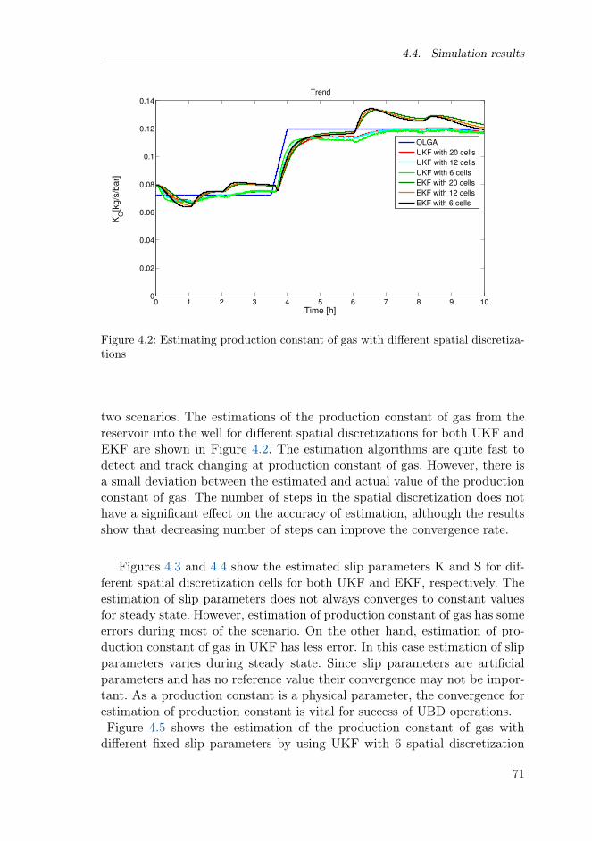
4.4. Simulation results
0 1 2 3 4 5 6 7 8 9 100
0.02
0.04
0.06
0.08
0.1
0.12
0.14
Time [h]
KG
[kg
/s/b
ar]
Trend
OLGA
UKF with 20 cells
UKF with 12 cells
UKF with 6 cells
EKF with 20 cells
EKF with 12 cells
EKF with 6 cells
Figure 4.2: Estimating production constant of gas with different spatial discretiza-tions
two scenarios. The estimations of the production constant of gas from thereservoir into the well for different spatial discretizations for both UKF andEKF are shown in Figure 4.2. The estimation algorithms are quite fast todetect and track changing at production constant of gas. However, there isa small deviation between the estimated and actual value of the productionconstant of gas. The number of steps in the spatial discretization does nothave a significant effect on the accuracy of estimation, although the resultsshow that decreasing number of steps can improve the convergence rate.
Figures 4.3 and 4.4 show the estimated slip parameters K and S for dif-ferent spatial discretization cells for both UKF and EKF, respectively. Theestimation of slip parameters does not always converges to constant valuesfor steady state. However, estimation of production constant of gas has someerrors during most of the scenario. On the other hand, estimation of pro-duction constant of gas in UKF has less error. In this case estimation of slipparameters varies during steady state. Since slip parameters are artificialparameters and has no reference value their convergence may not be impor-tant. As a production constant is a physical parameter, the convergence forestimation of production constant is vital for success of UBD operations.Figure 4.5 shows the estimation of the production constant of gas withdifferent fixed slip parameters by using UKF with 6 spatial discretization
71

4. State and parameter estimation of a Drift-Flux Model for Under-BalancedDrilling operations
0 1 2 3 4 5 6 7 8 9 10
1.12
1.14
1.16
1.18
1.2
1.22
Time [h]
Trend
K
UKF with 20 cells
UKF with 12 cells
UKF with 6 cells
EKF with 20 cells
EKF with 12 cells
EKF with 6 cells
Figure 4.3: Estimating slip parameter (K) for different spatial discretization cells
0 1 2 3 4 5 6 7 8 9 100.6
0.62
0.64
0.66
0.68
0.7
0.72
0.74
0.76
Time [h]
S
Trend
UKF with 20 cells
UKF with 12 cells
UKF with 6 cells
EKF with 20cells
EKF with 12 cells
EKF with 6 cells
Figure 4.4: Estimating slip parameter (S) for different spatial discretization cells
72
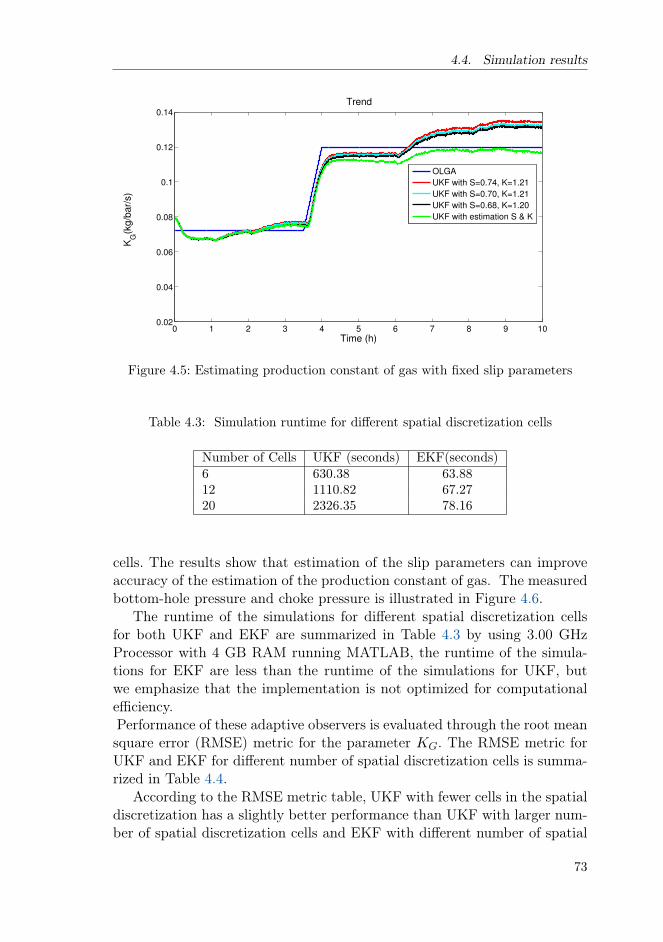
4.4. Simulation results
0 1 2 3 4 5 6 7 8 9 100.02
0.04
0.06
0.08
0.1
0.12
0.14
Time (h)
KG
(kg
/ba
r/s)
Trend
OLGA
UKF with S=0.74, K=1.21
UKF with S=0.70, K=1.21
UKF with S=0.68, K=1.20
UKF with estimation S & K
Figure 4.5: Estimating production constant of gas with fixed slip parameters
Table 4.3: Simulation runtime for different spatial discretization cells
Number of Cells UKF (seconds) EKF(seconds)6 630.38 63.8812 1110.82 67.2720 2326.35 78.16
cells. The results show that estimation of the slip parameters can improveaccuracy of the estimation of the production constant of gas. The measuredbottom-hole pressure and choke pressure is illustrated in Figure 4.6.
The runtime of the simulations for different spatial discretization cellsfor both UKF and EKF are summarized in Table 4.3 by using 3.00 GHzProcessor with 4 GB RAM running MATLAB, the runtime of the simula-tions for EKF are less than the runtime of the simulations for UKF, butwe emphasize that the implementation is not optimized for computationalefficiency.Performance of these adaptive observers is evaluated through the root meansquare error (RMSE) metric for the parameter KG. The RMSE metric forUKF and EKF for different number of spatial discretization cells is summa-rized in Table 4.4.
According to the RMSE metric table, UKF with fewer cells in the spatialdiscretization has a slightly better performance than UKF with larger num-ber of spatial discretization cells and EKF with different number of spatial
73

4. State and parameter estimation of a Drift-Flux Model for Under-BalancedDrilling operations
0 1 2 3 4 5 6 7 8 9 10200
220
240
260
280Trend
pbh[b
ar]
Time [h]
0 1 2 3 4 5 6 7 8 9 1060
80
100
120Trend
pc[b
ar]
Time [h]
OLGA
Figure 4.6: Bottom-hole pressure and choke pressure
Table 4.4: RMSE metric for estimate of KG
Number of Cells UKF EKF6 4.8× 10⁻³ 8.2× 10⁻³
12 4.8× 10⁻³ 8× 10⁻³
20 5.16× 10⁻³ 8.3× 10⁻³
discretization cells for PI estimation, although the number of cells in thespatial discretization does not have a significant effect on the accuracy ofestimation.
The second case study that is reported in this chapter considers UBDoperation of a vertical well drilled into an oil and gas reservoir. First thedrilling in a steady-state condition is initiated with the choke opening of 10%, then at t = 1 hour and 35 min the main pump is shut off to performa connection procedure, and the choke is closed to 6 %. The rotation ofthe drill string and the circulation of fluids are stopped for 15 mins. Nextafter making the first pipe connection at t = 1 hour and 50 min the mainpump and rotation of the drill string are restarted. After 1 hour and 45 min(i.e. 3 hour and 35 min), the choke is closed to 5 %, and the second pipeconnection procedure is started, and is completed after 15 mins. Then thechoke is opened to 10 % at t= 3 hours and 50 min. The measured bottom-hole pressure (pbh), choke pressure (pc), choke opening (Z), and mass flowrate of liquid from the drill string (wl,d) is illustrated in Figure 4.7.
74

4.4. Simulation results
0 0.5 1 1.5 2 2.5 3 3.5 4 4.5 5 5.5200
220
240
260Trend
Time [h]
pbh[b
ar]
0 0.5 1 1.5 2 2.5 3 3.5 4 4.5 5 5.50
5
10
15
wl,d(k
g/s
)
0 0.5 1 1.5 2 2.5 3 3.5 4 4.5 5 5.540
60
80
100
120
Time [h]
pc[b
ar]
0 0.5 1 1.5 2 2.5 3 3.5 4 4.5 5 5.50.04
0.06
0.08
0.1
0.12
Choke o
penin
g (
%)
Figure 4.7: Measured bottom-hole pressure, choke pressure, choke opening, andmass flow rate of liquid from the drill string for pipe connection scenario
Since these two scenarios model two drilling cases with different specifi-cations, different measurements and different parameters for each scenariowas used. Due to the fact that the liquid and gas flow rate at the outlet aresometimes measured by flow meter after separator, these measurements haveusually some delay. Also, these measurements are sometimes not available.Therefore, the purpose of the second scenario is to show how the estimatorworks without these measurements. This way we can answer a wide range ofproblems in UBD operation with choosing different measurements by usingthese two scenarios.
In the second scenario, it is assumed that only bottom-hole pressure(P (0)) and choke pressure (P (L)) are measured. The UKF and EKF esti-mate the states and production constants of gas and liquid (KG,KL). Slipparameters in this simulation are fixed (K = 1.15, S = 0.56). The parametervalues for the UKF for pipe connection scenario are the same as previousscenario. The initial values for the estimated and real parameters are asfollows:
KG = 0.07, KL = 0.1, KG = 0.091, KL = 0.13
The choke and the bottom-hole pressure measurements are corrupted by
75

4. State and parameter estimation of a Drift-Flux Model for Under-BalancedDrilling operations
zero mean additive white noise with the following covariance matrix
R =
[0.9 ∗ 0.42 0
0 0.9 ∗ 0.22
](bar2)
The covariance matrix for parameter variations uses in this simulation forboth EKF and UKF is
Qp = diag[4 ∗ 10−4, 2 ∗ 10−3], p = [KG,KL].
Figures 4.8 and 4.9 show the estimated production constants of gas andliquid from the reservoir into the well for different spatial discretization cellsfor both UKF and EKF, respectively.
The RMSE metric of the parameters KG and KL for UKF and EKF fordifferent spatial discretization cells after initial transient (t ≥ 0.5hour) aresummarized in Table 4.5. The results show that UKF and EKF with fewercells in the spatial discretization for the estimation of gas and liquid pro-duction constants have a better accuracy than UKF and EKF with largerspatial discretization cells with different spatial discretization cells for the es-timation of gas and liquid production constants during the pipe connection.Since the model is significantly less accurate during the pipe connection, weneed to prevent that the PI estimates drift away in order to compensate forother model errors. Hence, the Qp of UKF and EKF is 1000 times smallerthan the nominal value during the pipe connection. For the same reason, themeasurement covariance of UKF and EKF is tuned 1000 times larger thanthe nominal value during the pipe connection.
Table 4.5: RMSE metric for estimate of KG and KL for pipe connection scenario
Number of Cells KG (after t ≥ 0.5h) KL (after t ≥ 0.5h)UKF EKF UKF EKF
6 1.4× 10⁻³ 1.5× 10⁻³ 3.6× 10⁻³ 3.6× 10⁻³
12 1.8× 10⁻³ 2.2× 10⁻³ 3.8× 10⁻³ 3.8× 10⁻³
20 2.4× 10⁻³ 3.1× 10⁻³ 4.8× 10⁻³ 4.9× 10⁻³
Based on the RMSE metric in Table 4.5, UKF with fewer cells in thespatial discretization for the estimation of gas production constant (KG)has a slightly better performance than UKF with larger spatial discretizationcells and EKF with different spatial discretization cells for the estimation ofKG.
76

4.4. Simulation results
0 0.5 1 1.5 2 2.5 3 3.5 4 4.5 5 5.50.06
0.065
0.07
0.075
0.08
0.085
0.09
0.095
KG
[kg/s
/bar]
Trend
Time [h]
OLGAUKF with 20 cellsUKF with 12 cellsUKF with 6 cells
EKF with 20 cellsEKF with 12 cellsEKF with 6 cells
Figure 4.8: Estimating production constant of gas with different spatial discretiza-tion cells for pipe connection
0 0.5 1 1.5 2 2.5 3 3.5 4 4.5 5 5.50.095
0.1
0.105
0.11
0.115
0.12
0.125
0.13
0.135
0.14
0.145
KL[k
g/s
/bar]
Trend
Time [h]
OLGAUKF with 20 cellsUKF with 12 cellsUKF with 6 cells
EKF with 20 cellsEKF with 12 cellsEKF with 6 cells
Figure 4.9: Estimating liquid production constant with different spatial discretiza-tion cells for pipe connection
77

4. State and parameter estimation of a Drift-Flux Model for Under-BalancedDrilling operations
4.4.3 Robustness analysis of UKF and EKF in case ofuncertainties and errors in the reservoir and wellparameters of the model
Robustness of the adaptive observers is investigated in case of errors in thereservoir and well parameters of the model. This test is performed in case oferrors in the reservoir pore pressure and liquid density for pipe connectionscenario. The RMSE metric for UKF and EKF in the two cases of 1% erroron the reservoir pore pressure (pres,model = 282 bar) and 10% error on theliquid density (ρL,model = 1100 kg/m3)for different spatial discretizationcells after initial transient (t ≥ 0.5hour) are summarized in Table 4.6 and4.7, respectively.
Table 4.6: RMSE metric in case of error in the reservoir pressure value for pipeconnection scenario
Number of Cells KG (after t ≥ 0.5h) KL (after t ≥ 0.5h)UKF EKF UKF EKF
6 5.4× 10⁻³ 5.6× 10⁻³ 5.2× 10⁻³ 5.3× 10⁻³
12 5.8× 10⁻³ 6.0× 10⁻³ 6.0× 10⁻³ 6.0× 10⁻³
20 6.2× 10⁻³ 6.7× 10⁻³ 6.1× 10⁻³ 6.3× 10⁻³
Table 4.7: RMSE metric in case of error in the liquid density value for pipe con-nection scenario
Number of Cells KG (after t ≥ 0.5h) KL (after t ≥ 0.5h)UKF EKF UKF EKF
6 1.4× 10⁻³ 1.6× 10⁻³ 3.7× 10⁻³ 3.8× 10⁻³
12 1.9× 10⁻³ 2.2× 10⁻³ 3.9× 10⁻³ 3.9× 10⁻³
20 2.4× 10⁻³ 3.1× 10⁻³ 4.8× 10⁻³ 5.0× 10⁻³
Since the reservoir pore pressure has a direct effect on the mass flowrates from the reservoir into the well, small inaccuracies in the reservoir porepressure have a significant effect on the estimation of production constants.Therefor these methods with different number of spatial discretization cellsare very sensitive to errors in the reservoir pore pressure value. The resultsshow that UKF and EKF with different number of spatial discretization cellsare robust in case of error in the liquid density value of the model.
78

4.5. Conclusion
4.5 Conclusion
In this chapter, the joint UKF and EKF have been applied to the drift-fluxmodel for different spatial discretization cells to estimate the distributed un-measured states, geological properties of the reservoir (PI) and slip param-eters (S,K) during UBD operations using measurement of the bottom-holepressure and liquid and gas rate at the outlet. Furthermore, both produc-tion constants of gas and liquid and unmeasured states were estimated byusing only measurements of the choke and the bottom-hole pressures forthe pipe connection procedure. Simulation results demonstrated reasonableperformance of the joint UKF and EKF to detect and track a changinggas production coefficient using the simulated scenario with OLGA. Eventhough the simulation scenario is somewhat idealized the results are encour-aging. The number of spatial discretization cells was found to not have asignificant effect on accuracy of estimation. The UKF was also found to es-timate more accurately than the EKF. The results show that these methodsare very sensitive to errors in the reservoir pore pressure value.
79


CHAPTER5Design constrained MPC for heavedisturbance attenuation in offshoreManaged Pressure drilling systems
5.1 Introduction
In drilling operations, a drilling fluid (mud) is pumped down through the drillstring and flows through the drill bit at the bottom of the well (Figure 5.1).The mud flows up the well annulus carrying cuttings out of the well. The mudis separated at the surface from the return well flow, conditioned, and storedin storage tanks (pits) before it is pumped down into the well for furtherdrilling.To avoid fracturing, collapse of the well, or influx of formation fluidssurrounding the well, it is crucial to control the pressure in the open part ofthe annulus within a certain operating window. In conventional drilling, thisis done by using a mud of appropriate density and adjusting mud pump flowrates. In managed pressure drilling (MPD), the annulus is sealed, and themud exits through a controlled choke, allowing for faster and more precisecontrol of the annular pressure. In MPD operation, the dynamic pressure ofthe well must be kept higher than the reservoir pore pressure to prevent gasor formation fluids from entering the well and less than a formation fracturepressure at all times t and positions x.
pres(x) < pwell(x, t) < pfrac(x) (5.1)
where are reservoir pore pressure, well pressure, and formation fracture pres-sure, respectively. In automatic MPD systems, the choke is controlled tokeep the annular mud pressure between specified upper and lower limits.There are several studies about different aspects of MPD modeling (e.g.,see [38, 48, 50, 63, 96]). Estimation and control design in MPD have beeninvestigated by several researchers (e.g., see [12, 25, 38, 83, 113, 114]). These
81

5. Design constrained MPC for heave disturbance attenuation in offshoreManaged Pressure drilling systems
studies are mainly focused on pressure control during drilling from a fixedplatform without any heave motion.
The automatic MPD system has several advantages compared to conven-tional drilling as follows:• Reducing the drilling costs as a result of reducing the nonproductivetime.• Increasing the rate of penetration.• Improving well-bore stability.• Minimizing the risk of lost circulation.• Extending control over bottom-hole pressure (BHP) to operational sce-narios such as connections and trips and when the rig pumps are off.• Improvement in safety and well control resulting from more detaileddesign and planning required for accomplishment.
When designing MPD control systems, one should take into account var-ious operational procedures and disturbances that affect the pressure in-side the well. There is a specific disturbance occurring during drilling fromfloaters that significantly affects MPD operations. In this case, the rig movesvertically with the waves, referred to as heave motion. As drilling proceeds,the drill string needs to be extended with new sections. Thus, every coupleof hours or so, drilling is stopped to add a new segment of about 27 m tothe drill string. During drilling, a heave compensation mechanism is activeto isolate the drill string from the heave motion of the rig. However, duringconnections, the pump is stopped, and the string is disconnected from theheave compensation mechanism and rigidly connected to the rig. The drillstring then moves vertically with the heave motion of the floating rig andacts like a piston on the mud in the well. The heave motion may be morethan 3 m in amplitude and typically has a period of 10–20 s, which causessevere pressure fluctuations at the bottom of the well. Pressure fluctuationshave been observed to be an order of magnitude higher than the standardlimits for pressure regulation accuracy in MPD (about ±2.5 bar) [24]. Down-ward movement of the drill string into the well increases pressure (surging),and upward movement decreases pressure (swabbing). Excessive surge andswab pressures can lead to mud loss resulting from high-pressure fracturingof the formation or a kick-sequence (uncontrolled influx from the reservoir)that can potentially grow into a blowout as a consequence of low pressure.
Hauge et al.[30] designed an adaptive observer to estimate the unknownstates, the magnitude and location of the in /out flux and parameters ofthe hydraulic system during MPD. It is also used control law for choke toattenuate the in/out flux during drilling. This adaptive observer is verifiedwith several experimental and simulation results. Carlsen et al.[13] designed
82
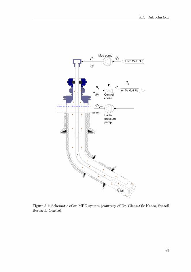
5.1. Introduction
Figure 5.1: Schematic of an MPD system (courtesy of Dr. Glenn-Ole Kaasa, StatoilResearch Centre).
83

5. Design constrained MPC for heave disturbance attenuation in offshoreManaged Pressure drilling systems
linear MPC, PI and internal model controller based on simple first ordermodel to stabilize the well pressure during MPD operations. The perfor-mance of these controllers was evaluated on three different drilling scenarioswhile the well kicked during these scenarios. Manipulated variables in thelinear MPC and the internal model controller are choke valve and pump.while manipulated variable in the PI is only choke valve. The simulationsshow that the controllers have a good performance to stabilize the well pres-sure in case of change in drilling conditions and disturbances. Asgharzadehet al.[7] designed nonlinear MPC (NMPC) with adaptive observer for kickdetection and attenuation, regulation of the bottom hole pressure and rateof penetration (ROP) with direct pressure measurements from wired pipetelemetry technology during MPD. This Controller works for both normaldrilling and kick event. Some parameters of the drilling model drilling couldnot be measured directly. Therefore, the annulus friction factor and densityis estimated by a nonlinear moving horizon estimator. In this case the gasinflux flow rate is estimated by an extended Kalman filter with measure-ment of choke valve, down-hole and pump pressures. Manipulated variablesin the NMPC are mud pump flow rate, choke valve position, drill string ro-tation rate, and weight-on-bit (WOB). The objective function of the NMPCis using an `1norm instead of conventional squared error norm for betternoise and drift rejection. Asgharzadeh et al.[6] studied effect of temporarilycommunication loss in the NMPC during kick event. This paper shows thatdistributed pressure measurements with multiple sensor can improve kickattenuation of NMPC during kick event due to availability of a sensor closerto the influx location [6].
Rasmussen et al.[99] compared and evaluated different MPD methodsfor the compensation of surge and swab pressure. In Nygaard et al. [86],it is shown that surge and swab pressure fluctuation in the BHP duringpipe connection can be suppressed by controlling the choke and main pump.Nygaard et al. [87] used a nonlinear model predictive control (MPC) al-gorithm to obtain optimal choke pressure for controlling the BHP duringpipe connection in a gas-dominant well. Pavlov et al. [93] presented twononlinear control algorithms for handling heave disturbances in MPD oper-ations. Mahdianfar et al. [61, 62] designed an infinite-dimensional observerthat estimates the heave disturbance. This estimation is used in a controllerto reject the effect of the disturbance on the downhole pressure. In all theabove mentioned papers, the controllers are designed for the nominal casedisregarding the uncertainty in the parameters, although several parametersin the well could be uncertain during drilling operations. In addition, theheave disturbance, which is inherently stochastic and contains many differ-ent harmonics, is approximated by one or a couple of sinusoidal waves with
84

5.2. Mathematical Modeling
known fixed frequencies throughout controller design and simulations. Inthis chapter, a stochastic model for the heave motion in the North Sea isgiven and is used in simulations.
MPC is one of the most popular controller design methodologies for com-plex constrained multivariable control problems in the industry and has beenthe subject of many studies since the 1970s(e.g. see [23, 60, 64, 67]). At eachsampling time, an MPC control action is acquired by the online solution ofa finite horizon open-loop optimal control problem. Only the first part ofthe optimal control trajectory is applied to the system. At the next sam-pling time, the computation is repeated with new measurements obtainedfrom the system. The purpose of this chapter is to study a constrained MPCscheme for controlling the pressure during MPD oil well drilling using mea-surements and optionally predictions of the heave disturbances. In somecases, short-term heave motion prediction based on forward-looking sensorssuch as ocean wave radar may be predictable [44], and we can use themdirectly in our MPC controller. One of the criteria for evaluating the con-troller performance is its ability to handle heave disturbances. This schemeis compared with a standard proportional-integral-derivative (PID) controlscheme. Furthermore, the robustness of the controller to deal with heavedisturbances despite significant uncertainties in the friction factor and bulkmodulus is investigated by Monte Carlo simulations.
In the following sections, a model based on mass and momentum balancesthat provides the governing equations for pressure and flow in the annulusis given. A stochastic modeling of waves in the North Sea is used, and theheave disturbance induced by the elevation motion of the sea surface ismodeled. The design of a constrained MPC scheme is presented and appliedon MPD. In the cases with and without the predictive heave disturbancefeed-forward and prediction, it is shown that this controller outperforms aPID controller. Finally robust performance of an MPC controller is evaluatedthrough Monte-Carlo simulations.
5.2 Mathematical Modeling
In this section, the distribution of single-phase flows and pressures in theannulus and the drill string is modeled by two coupled partial differentialequations (PDEs). Then, the PDE model is discretized by using the finitevolume method. Finally, the model describing the vessel’s heave motion inresponse to the stochastic sea waves in the North Sea is presented and usedas the heave disturbance.
85

5. Design constrained MPC for heave disturbance attenuation in offshoreManaged Pressure drilling systems
5.2.1 Annulus flow dynamics
The governing equations for flow in an annulus are derived from mass andmomentum balances based on 1-D hydraulic transmission line [50].
∂p
∂t= − β
A
∂q
∂x(5.2)
∂q
∂t= −A
ρ0
∂p
∂x− F
ρ0+Ag cos(α(x)) (5.3)
where p(x, t) and q(x, t) are the pressure and volumetric flow rate at locationx and time t, respectively. The bulk modulus of the mud is denoted by β.A(x) is the cross section area, ρ is the (constant) mass density, F is thefriction force per unit length, g is the gravitational constant and α(x) is theangle between gravity and the positive flow direction at location x in thewell (Figure 5.2). To derive a set of ordinary differential equations describingthe dynamics of the pressures and flows at different positions in the well,equations (5.2) and (5.3) are discretized by using a finite volumes method. Tosolve this problem, the annulus is divided into a number of control volumes,as shown in Figure 5.2, and integrating (5.2) and (5.3) over each controlvolume. This model will be used for the MPC design.
Landent et al. [50] found that five control volumes could capture themain dynamics of the system in the case of heave disturbance for a wellfrom the Ullrigg test facility with a particular length of about 2,000 m andwith water-based mud. Ullrigg is a full scale drilling test facility located atthe International Research Institute of Stavanger (IRIS). The parameterscorresponding to that well are used as a base case throughout this chapter.The set of nine ordinary differential equations describing five control volumesin the annulus are shown below ([48, 49])
p1 =β1A1l1
(−q1 − vdAd) (5.4)
p2 =β2A2l2
(q1 − q2) (5.5)
p3 =β3A3l3
(q2 − q3) (5.6)
p4 =β4A4l4
(q3 − q4) (5.7)
p5 =β5A5l5
(q4 − qc + qbpp) (5.8)
86

5.2. Mathematical Modeling
volume. This derivation is done similar to the one done in[10].
To incorporate the important pressure dynamics createdby the drill string movement, there are two things to bearin mind: First, the volume of the annulus will continuouslychange by vd(t)Ad, where Ad is the drill string cross sectionarea, due to the top of the drill string moving in and out ofthe well with velocity vd. Second, one also has to considerthe fact that the cross section of the drill bit will in generalbe larger than that of the rest of the drill string. This willcause the generated flow to be “squeezed” in over a smallercross section, increasing the velocity and thus also the frictionaround the drilling bit. (See also Figure 2.) Taking all theseissues into account, the finite volume method results in thefollowing set of equations
p1 =�1
A1l1(�q1 � vdAd)
pi =�i
Aili(qi�1 � qi) , i = 2, 3, .., N � 1
pN =�N
AN lN(q(N�1) � qc + qbpp) (3)
qi =Ai
li⇢i(pi � pi+1) �
Fi (qi) Ai
⇢ili� Aig
�hi
li,
i = 1, 2, ..N � 1 (4)
Here, the numbers 1...N refer to control volume number,with 1 being the lower most control volume representingthe down hole pressure (p1 = pbit), and N being the uppermost volume representing the choke pressure (pN = pc). Thelength of each control volume is denoted l, and the heightdifference is �h. Notice that since the well may be non-vertical, l and �h may in general differ from each other. Toour disposal for control are the back pressure pump flow qbpp
and the choke flow qc. The flow from the back pressure pumpqbpp is linearly related to the pump frequency and cannot bechanged fast enough to compensate for the heave-inducedpressure fluctuations. Therefore, it is the choke flow thatis used primarily for control. It is modelled by an orificeequation:
qc = Kc
ppc � p0G (u) (5)
Here, Kc is the choke constant corresponding to the areaof the choke and the density of the drilling fluid. p0 is the(atmospheric) pressure down stream the choke and G(u) is astrictly increasing and invertible function relating the controlsignal to the actual choke opening, taking its values on theinterval [0, 1].
B. Friction Model
To model the friction force acting on each control volume,we propose to use standard, Newtonian friction factor correla-tions (see e.g. [12] for details). This is due to the observationsfrom measurement data from full scale tests [1] that suggestthe friction force in the annulus is a linear function of the
A
qN-1
qN-2
qc
p1
q1
β,ρ
pN-1
pN
qbpp
α
g
x
l=Δh
DrillString
DrillingBit
Figure 2. Control volumes of annulus hydraulic model.
flow rate, at least for the modest flow rates that can beexpected without externally forced flow (zero flow from themain pump). This corresponds well to Newtonian frictionfactors for laminar flow. See Figure 3 for the measured steadystate friction drops.
0 0.005 0.01 0.015 0.02 0.0250
5
10
15
20
25
30
35
40
45
50
q (m3/s)
p (
bar)
drill stringannulus
Figure 3. Friction losses from observed, full scale testing data
Taking the special geometry of the annulus region intoaccount, it has been proposed [13] to use a modified Reynoldsnumber to calculate the friction factor. However, to keepthe detail level manageable, we will in this paper lump theentire friction model into a constant (or, more likely, slowlyvarying) friction coefficient kfric, giving the resulting friction
Figure 5.2: Control volumes of annulus hydraulic model [50]
qi =Ailiρi
(pi − pi+1)−Fi(qi)Ailiρi
−Aig∆hili
(5.9)
qc = Kc√pc − p0G(u) (5.10)
where, i = 1, ..., 4, and the numbers 1, ..., 5 refer to control volume number,with 1 being the lower most control volume representing the down hole pres-sure (p1 = pbit), and 5 being the upper most volume representing the chokepressure (p5 = pc). vd is the heave vertical velocity due to ocean waves. Thelength of each control volume is denoted by l, and the height difference is∆hi. Since the well may be non-vertical, li and ∆hi may in general differfrom each other. The means for pressure control are the back pressure pumpflow qbpp and the choke flow qc.The flow from the back pressure pump qbpp islinearly related to the pump frequency and cannot be changed fast enough tocompensate for the heave-induced pressure fluctuations. Therefore, it is the
87

5. Design constrained MPC for heave disturbance attenuation in offshoreManaged Pressure drilling systems
choke flow that is used primarily for control, which is modeled by nonlinearorifice equation 5.10. Kc is the choke constant corresponding to the area ofthe choke and the density of the drilling fluid. p0 is the (atmospheric) pres-sure downstream the choke and G(u) is a strictly increasing and invertiblefunction relating the control signal to the actual choke opening, taking itsvalues on the interval [0, 1].
Based on experimental results from full scale tests at Ullrigg, the frictionforce in the annulus is considered to be a linear function of the flow rate[50]. Friction force on the ith control volume is approximately modeled as
Fi(qi) =kfricqiAi
(5.11)
where kfric is the constant friction coefficient.Some components of the transient hydraulic model, equations (5.2) -
(5.3), have significant uncertainties, such as the following [63]:
� Rheology and viscosity of drilling fluid: Most drilling fluids arenon-Newtonian, that is, with a nonlinear relation between shear stressand shear rate. Consequently, the viscosity will not be constant overa cross-sectional flow area. To measure the shear stress-shear rate re-lationship, the viscometer measurements must be correlated with therheological model applied. However, information is limited and nor-mally inadequate for a model of high accuracy, particularly for modernoil-based muds. Also, viscosity may depend on pressure and tempera-ture. Manual rheology measurements are normally performed period-ically on the rig at the atmospheric pressure and temperature of themud in the pit. Thus, information on the influence of temperature andpressure variations is missing [21, 27, 53].
� Frictional pressure loss models for drill pipe and annulus:The frictional pressure loss depends on the mean cross-sectional veloc-ity, drilling fluid viscosity, flow regime, hydraulic diameter, and piperoughness. The accuracy of all these derived parameters is question-able. Moreover, the Fanning friction factor is a function of Reynoldsnumber where the Reynolds number is a function of the fluid viscosityfor a characteristic diameter [21, 38, 53].
� Effective bulk modulus: A bulk modulus is used because the degreeof mechanical compliance of casing, pipe, hoses, and other componentsis uncertain and also because it is impossible to predict the amount ofgas pockets, bubbles, or breathing of the well [38].
88

5.2. Mathematical Modeling
5.2.2 Waves Response Modeling
Environmental forces in the vertical direction due to waves are considereddisturbances to the motion control system of floating vessels. These forces,which can be described in stochastic terms, are conceptually separated intolow-frequency (LF) and wave-frequency (WF) components, [22]. The LFpart is not considered any farther since it is very slow compared to thedynamics of the mud circulation system and dealt with by other controllersand operationally (e.g., pipe connection).
During normal drilling operations, the WF part of the drill-string motionis compensated by the heave control system ,[16, 42, 44]. However, duringconnections, the drill string is disconnected from the heave compensationmechanism and rigidly connected to the rig. Thus, it moves vertically withthe heave motion of the floating rig and causes severe downhole pressurefluctuations.
Linear Approximation for WF Position
When simulating and testing feedback control systems, it is useful to havea simple and effective way of representing the wave forces. Here, the motionresponse amplitude operators(RAOs) are represented as a state-space modelwhere the wave spectrum is approximated by a linear filter. In this setting,the RAO vessel model is represented in Figure 5.3, where Hrao(s) is thewave amplitude-to-force transfer function and Hv(s) is the force-to-motiontransfer function. In addition to this, the response of the motion RAOs andthe linear vessel dynamics in cascade is modeled as constant tunable gains,[22]. This means that the RAO vessel model is approximated as (Figure 5.3)
K = diag{K1,K2,K3,K4,K5,K6} (5.12)
Hrao(s)Hv(s) ≈ K (5.13)
Ak τwave1Hv(s)Hrao(s)Hs(s)
w ηw
Figure 5.3: Linear approximation for computation of wave-induced positions.
Since the vessel is typically designed to avoid resonances in the dominantWF, the fixed-gain approximation [equation 5.13] produces good results ina closed-loop system where the purpose is to test the robustness and perfor-mance of a feedback control system in the presence of waves.
89

5. Design constrained MPC for heave disturbance attenuation in offshoreManaged Pressure drilling systems
Then, the generalized WF position vector ηw in Figure 5.3 becomes
ηw = KHs(s)w(s) (5.14)
where Hs(s) is a diagonal matrix containing transfer function with the spec-tral factors of the wave spectrum S(ω). The WF position for the degree offreedom related to heave motion becomes
ηhw = Khξh (5.15)
ξh(s) = hh(s)wh(s) (5.16)
where hh(s) is the spectral factor of the wave spectral density function S(ω)and wh(s) is a zero-mean Gaussian white noise process with unity poweracross the spectrum:
P hww(ω) = 1.0 (5.17)
Hence, the power spectral density (PSD) function for ξh(s) can be computedas
P hξξ(ω) = |hh(jω)|2P hww(ω) = |hh(jω)|2 (5.18)
Joint North SeaWave Project Spectrum
The Joint North Sea Wave Project (JONSWAP) formulation is based on anextensive wave measurement program known as the JONSWAP carried outin 1968 and 1969 in the North Sea, between the island Sylt in Germany andIceland. The JONSWAP spectrum is representative of wind-generated wavesunder the assumption of finite water depth and limited fetch [22, 90].Thespectral density function is written as
S(ω) = 155H2s
T 41
ω−5 exp(−944
T 41
ω−4)γY (5.19)
where Hs is the significant wave height, T1 is the average wave period,γ = 3.3 and
Y = exp
[−(0.191ωT1 − 1√
2σ
)2](5.20)
where
σ =
{0.07 for ω ≤ 5.24/T1
0.09 for ω > 5.24/T1(5.21)
The modal period, T0, is related to the average wave period through T1 =0.834T0, [22].
Figure 5.4, produced using MSS Toolbox, shows the JONSWAP spectrumpower distribution curve. The parameter values forHs and T0 are taken from
90

5.2. Mathematical Modeling
[66]. From Figure 5.4, we can see that the JONSWAP spectrum is a narrowband spectrum, and its energy is mainly focused on 0.5− 1.5 rad/s, and thepeak frequency is ω0 = 0.7222 rad/s.
0.5 1 1.5 2 2.50
0.5
1
1.5
2
2.5
3
3.5
4JONSWAP Spectrum
[rad/s]
S() [
m2 s
]
JONSWAP spectrumLinear approximation
Figure 5.4: JONSWAP spectrum and its approximation.
Second-Order Wave Transfer Function Approximation
As discussed earlier, a finite dimensional,rational transfer function wave re-sponse approximation for Hs(s) is usually preferred by ship control systemsengineers, because of its simplicity and applicability:
hh(s) =2λω0σs
s2 + 2λω0s+ ω20
(5.22)
where λ = 0.1017, σ = 1.9528, Hs = 4.70, T0 = 8.70, ω0 = 0.7222, andKh = 9.1 are typical parameters for heave motion of the drilling rig. Thetransfer function approximation is shown in Figure 5.4.
91

5. Design constrained MPC for heave disturbance attenuation in offshoreManaged Pressure drilling systems
5.3 Controller Design
The model described by equations (5.4)-(5.10) is in form of a nonlinear strictfeedback system, with an unmatched stochastic disturbance. By consideringaj =
βjAj lj
, bj =Aj
ljρj, cj =
Kfric
ρj lj, the model in state-space form would be
{X = AX +Bua +B1 + Edy = CX
(5.23)
where
X =[p1 q1 p2 q2 p3 q3 p4 q4 p5
]T
A =
0 −a1 0 0 0 0 0 0 0b1 −c1 −b1 0 0 0 0 0 00 a2 0 −a2 0 0 0 0 00 0 b2 −c2 −b2 0 0 0 00 0 0 a3 0 −a3 0 0 00 0 0 0 b3 −c3 −b3 0 00 0 0 0 0 a4 0 −a4 00 0 0 0 0 0 b4 −c4 −b40 0 0 0 0 0 0 a5 0
B =
[0 0 0 0 0 0 0 0 a
]TB1 = −263.7814
[0 1 0 1 0 1 0 1 0
]TE =
[−22.0857 0 0 0 0 0 0 0 0
]TC =
[1 0 0 0 0 0 0 0 0
](5.24)
and
ua = qbpp − qc (5.25)
The output y = p1 is the BHP. The heave disturbance vd in equation (5.4)will be compensated by using constrained MPC as designed in the followingsection. Note that the hydrostatic pressures in equation (5.9) are includedin the states pi in (5.4)-(5.8).
5.3.1 MPC
The main MPC objective in this chapter is to regulate BHP to desiredvalues (set points) during pipe connection by minimizing the cost functionand satisfying output and input constraints.
92
5.3. Controller Design
Constrained MPC design
Consider the discrete-time linear time-invariant input-affine system [equa-tion 5.23] while fulfilling the constraints
ymin ≤ y(k) ≤ ymax, umin ≤ u(k) ≤ umax (5.26)
at all time instants k ≥ 0.In (5.23)-(5.26), n , p and m are the number of states, outputs and inputsrespectively, and x(k) ∈ <n , y(k) ∈ <p , d(k) ∈ <n and u(k) ∈ <m are thestate, output, disturbance and input vectors respectively.
The constrained MPC solves a constrained optimal regulation problemat each time k.
minU
∆={uk,··· ,uk+N}
{J(u, y, r) =N∑i=1
[(uTk+i|kRuk+i|k + ∆uTk+i|kRδu∆uk+i|k
+ (yk+i|k − rk+i|k)TQ(yk+i|k − rk+i|k)]}
subjectto ymin ≤ yi+k|k ≤ ymax i = 1, · · · , N,umin ≤ ui+k|k ≤ umax i = 1, · · · , N,∆umin ≤ ∆ui+k|k ≤ ∆umax i = 1, · · · , N,xk|k = x(k) (5.27)
xi+k+1|k = Adixi+k|k +Bdiui+k|k +Bdi,1 + Edidi+k|k,
yi+k|k = Cdixi+k|k
where N, J and r are the finite horizon, cost function and reference tra-jectory, respectively. The matrices Adi, Bdi, Bdi,1, Edi, and Cdi follow froma discretization of the system. The subscript "(k + i|k)" denotes the valuepredicted for time k+ i, and it is assumed that Q,Rδu and R are the positivedefinite matrices.
Since the states xk are not directly measurable, predictions are computedfrom the estimation of states. Since the pair (C,A) is detectable, a stateobserver is designed to provide estimation of states xk, as described in theKalman Filter for State Estimation section. The controller computes the op-timal solution U by solving the quadratic programing (QP) [ equation 5.27].If the future value of disturbances and/or measurement of disturbances arenot assumed to be known, then disturbances are assumed to be zero in theMPC predictions.
93

5. Design constrained MPC for heave disturbance attenuation in offshoreManaged Pressure drilling systems
Controller parameters such as weight of inputs, inputs’ rate, and outputsand control horizon must be tuned to achieve the good performance andstability in this problem. The prediction horizon should be chosen largeenough to ensure the closed-loop stability of the control system.
MPC Constraints
The upper and lower bounds on the input are chosen from the choke open-ing modes, which are fully opened and fully closed, respectively. Enforcingpressure of the annulus in a certain operating window is the main reason forusing MPD. The hydrostatic pressure of the well must be kept between boththe reservoir formation pressure and collapsing pressure on one side and thefracturing pressure on the other side. The typical limit for pressure regula-tion accuracy in MPD is about ±2.5 bar. The controlled output constraintsfor the limits for pressure regulation accuracy in MPD must be softened bythe addition of slack variables.
MPC Cost Function
The cost function [ equation 5.27] consists of three standard terms. The firstterm penalizes the prediction input effort, and the second term in the costfunction penalizes variation in the prediction control input. The last termweights the deviations of the output variable from the reference trajectoryrk+i|k.
5.3.2 Kalman Filter for state estimation
The discrete-time Kalman filter is a recursive algorithm based on discretelinear dynamic systems and known stochastic models of noise and distur-bance. The Kalman filter has the ability to estimate states with the minimumvariance of the estimation error. This algorithm has two distinct steps: pre-diction and correction. In the prediction step, predicted state (xk|k−1) andpredicted estimate covariance (Pk|k−1) are computed. In the correction stepwith updated measurement, optimal Kalman gain (Kk) is computed. Then,the updated state (xk|k ) and updated estimate covariance (Pk|k) are com-puted with optimal Kalman gain. More details on Kalman filtering can befound in [104].
5.4 Simulation Results
The nominal parameters for simulations, identified from the IRIS drill sim-ulator [89], are given in Table 5.1.
94
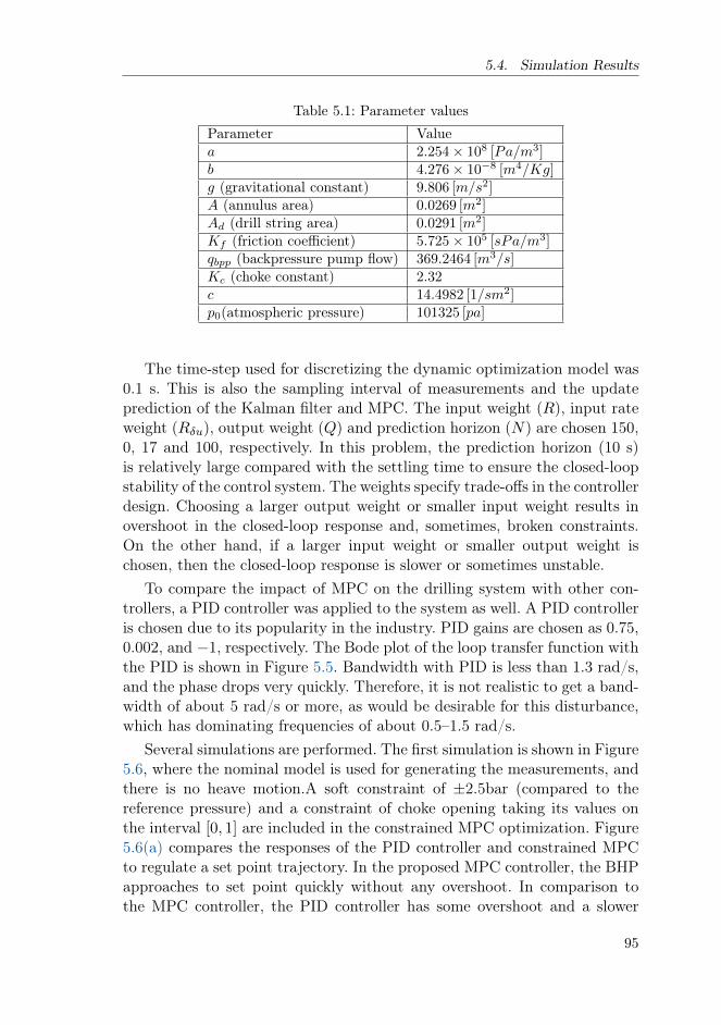
5.4. Simulation Results
Table 5.1: Parameter values
Parameter Valuea 2.254× 10⁸ [Pa/m3]b 4.276× 10⁻⁸ [m4/Kg]g (gravitational constant) 9.806 [m/s2]A (annulus area) 0.0269 [m2]Ad (drill string area) 0.0291 [m2]Kf (friction coefficient) 5.725× 10⁵ [sPa/m3]qbpp (backpressure pump flow) 369.2464 [m3/s]Kc (choke constant) 2.32c 14.4982 [1/sm2]p0(atmospheric pressure) 101325 [pa]
The time-step used for discretizing the dynamic optimization model was0.1 s. This is also the sampling interval of measurements and the updateprediction of the Kalman filter and MPC. The input weight (R), input rateweight (Rδu), output weight (Q) and prediction horizon (N) are chosen 150,0, 17 and 100, respectively. In this problem, the prediction horizon (10 s)is relatively large compared with the settling time to ensure the closed-loopstability of the control system. The weights specify trade-offs in the controllerdesign. Choosing a larger output weight or smaller input weight results inovershoot in the closed-loop response and, sometimes, broken constraints.On the other hand, if a larger input weight or smaller output weight ischosen, then the closed-loop response is slower or sometimes unstable.
To compare the impact of MPC on the drilling system with other con-trollers, a PID controller was applied to the system as well. A PID controlleris chosen due to its popularity in the industry. PID gains are chosen as 0.75,0.002, and −1, respectively. The Bode plot of the loop transfer function withthe PID is shown in Figure 5.5. Bandwidth with PID is less than 1.3 rad/s,and the phase drops very quickly. Therefore, it is not realistic to get a band-width of about 5 rad/s or more, as would be desirable for this disturbance,which has dominating frequencies of about 0.5–1.5 rad/s.
Several simulations are performed. The first simulation is shown in Figure5.6, where the nominal model is used for generating the measurements, andthere is no heave motion.A soft constraint of ±2.5bar (compared to thereference pressure) and a constraint of choke opening taking its values onthe interval [0, 1] are included in the constrained MPC optimization. Figure5.6(a) compares the responses of the PID controller and constrained MPCto regulate a set point trajectory. In the proposed MPC controller, the BHPapproaches to set point quickly without any overshoot. In comparison tothe MPC controller, the PID controller has some overshoot and a slower
95

5. Design constrained MPC for heave disturbance attenuation in offshoreManaged Pressure drilling systems
−500
−400
−300
−200
−100
0
100
Ma
gn
itu
de
(d
B)
10−4
10−3
10−2
10−1
100
101
102
103
−900
−720
−540
−360
−180
0
Ph
ase
(d
eg
)Bode Diagram
Gm = 11.8 dB (at 1.23 rad/s) , Pm = 59.7 deg (at 0.32 rad/s)
Frequency (rad/s)
Figure 5.5: Bode plot of the loop transfer function with the PID.
response. The choke control signal in the constrained MPC is illustrated inFigure 5.6(b).
The second simulation is shown in Figures 5.7 and 5.8, where the nomi-nal model with heave disturbance is used for generating the measurements.The same constraints as in previous simulation are enforced to the con-troller. Figure 5.7 compares the responses of constant input (qbpp = qc) andconstrained MPC to track the set point reference with existing heave dis-turbance. A constant input couldn’t reduce the effect of heave disturbanceand track the set point reference. Figure 5.8(a) compares the responses ofPID controller and constrained MPC to track the set point reference with aheave disturbance. It is found that the MPC controller is capable of main-taining the constraints, whereas the PID controller is not. Performance ofthe controller is evaluated through the root mean square (RMS) trackingerror metric. The RMS tracking errors for the MPC and PID controllers are1.2524 and 1.6273, respectively, which means that the effect of disturbancesis reduced to 77.0% by the MPC compared to the PID. As indicated inthis figure and the RMS tracking error, the constrained MPC shows gooddisturbance rejection capabilities. The choke control signal is illustrated in
96

5.4. Simulation Results
0 10 20 30 40 50 60257
258
259
260
261
262
263
264
265
266
Time (s)
Pre
ssure
(bar)
Bottom−hole pressure
PID
MPC
(a) Bottom-hole pressure without disturbance.
0 10 20 30 40 50 600.26
0.28
0.3
0.32
0.34
0.36
0.38
0.4
0.42
0.44
Time (s)
Choke o
penin
g
Choke Input
(b) MPC control signal to the choke without disturbance.
Figure 5.6: Output and control signal of MPC without disturbance.
97

5. Design constrained MPC for heave disturbance attenuation in offshoreManaged Pressure drilling systems
Figure 5.8(b). Figure 5.9 shows heave disturbance pressure variations.
0 50 100 150 200250
252
254
256
258
260
262
264
266
268
270
Time(s)
Pre
ssure
(bar)
Bottom−hole Pressure
Constant Input
Constrained MPC
Figure 5.7: Bottom-hole pressure
The next simulation is shown in Figure 5.10 where the nominal modelwith heave disturbance is used for generating the measurements. The sameconstraints as in the previous simulation are enforced to the controller. Inthis simulation, the heave disturbance is assumed to be predictable. Theheave disturbance is given by vd = cos(2πt/12)[m], where 2π/12 correspondsclosely to the most dominant wave frequency in the North Atlantic, withreference to the JONSWAP spectrum [49, 50]. The input weight for MPCwith future knowledge of heave disturbance is chosen R = 85. Figure 5.10compares the responses of MPC controller without future knowledge of heavedisturbance and MPC with future knowledge of heave disturbance to trackthe set point reference. It is found that the MPC controller with futureknowledge of heave disturbance reduces the effect of heave disturbance moresignificantly than the MPC controller without future knowledge of heavedisturbance. The MPC can therefore efficiently utilize predictions of futureheave disturbance to improve the control.
98

5.4. Simulation Results
0 20 40 60 80 100 120 140 160 180 200256
258
260
262
264
266
268
270
Time (s)
Pre
ssure
(bar)
Bottom−hole pressure
MPC
PID
(a) Bottom-hole pressure with heave disturbance.
0 20 40 60 80 100 120 140 160 180 2000.26
0.28
0.3
0.32
0.34
0.36
0.38
0.4
0.42
0.44
0.46
Time (s)
Choke o
penin
g
Choke input
(b) MPC control signal to the choke with heave disturbance.
Figure 5.8: Output and control signal of MPC with heave disturbance.
99

5. Design constrained MPC for heave disturbance attenuation in offshoreManaged Pressure drilling systems
0 20 40 60 80 100 120 140 160 180 200−15
−10
−5
0
5
10
15
Time(s)
Pre
ssure
(bar)
Figure 5.9: Heave disturbance
0 20 40 60 80 100 120 140 160 180 200254
256
258
260
262
264
266
268
Time (s)
Pre
ssure
( b
ar
)
Bottom−hole pressure
MPC without future knowledge of disturbance R=150
MPC with future knowledge of disturbance R=85
Figure 5.10: Bottom-hole pressure with predictable heave disturbance.
100
5.5. Conclusions
5.4.1 Robustness Analysis of Closed-Loop System Using MonteCarlo Simulations
Finally, the robustness of the constrained MPC without future knowledgeof heave disturbance with the presence of uncertainties in the friction fac-tor and bulk modulus, 25% each, is evaluated by Monte Carlo simulations.Each simulation time was 200 s, and the simulations were done over 400Monte Carlo runs in the uncertainty region with uniform distribution. Weevaluated the performance by computing the ratio of average of RMS ofthe tracking error to RMS of the stochastic disturbance. The result indi-cates that the controller was successful to attenuate the disturbance in theuncertain system to 74.34%.
5.5 Conclusions
In this chapter, a dynamical model describing the flow and pressure in theannulus is used. The model was based on a hydraulic transmission line andis discretized using a finite volume method. The disturbance due to drillstring movement is simulated as a stochastic model describing sea waves inthe North Sea applied to the flow in the bottom hole of the well.
A constrained MPC for controlling bottom-hole pressure during oil welldrilling was designed. It was found that the constrained MPC scheme is ableto successfully control the downhole pressure. It was also found that a con-strained MPC shows improved attenuation of heave disturbance. Comparingthe PID controller results with MPC shows that the MPC controller has abetter performance than the PID controller, being able to reduce the effectof disturbances to 77%. Monte Carlo simulations show that the constrainedMPC has a good performance to regulate the set point and attenuate theeffect of the heave disturbance in case of significant uncertainties in thewell parameter values. Finally, it is shown that performance can be furtherimproved by prediction of the heave motion about 10 s into the future.
101


CHAPTER6Conclusions and suggestions for future
work
The final chapter presents the conclusions that can be drawn from the workof this thesis, and gives possible directions for future work.
6.1 Conclusions
Since the oil production in Norway decreased from 3.22 million (B/D) in2001 to 1.46 million (B/D) in 2013 1, the number of depleted reservoirs andformations with low pressure margins in Norway have increased. In orderto increase recovery, it is very vital to invest in developing advanced tech-nologies which can be utilized for depleted reservoir and formations withnarrow pressure window. Underbalanced drilling (UBD) and Managed pres-sure drilling (MPD) are drilling technologies which has been developed towork on challenging reservoir and reducing drilling problems. In order to fur-ther advance these technologies, the objectives of this work are to estimatethe states and geological properties of the reservoir during UBD operation,and design of a controller to attenuate heave disturbance in offshore MPDsystem.Novel methods has been designed and developed to estimate reservoir prop-erties with using only pressure measurements and different lumped and dis-tributed models. Meanwhile, methods to control the pressure during MPDoil well drilling using measurements and predictions of the heave disturbancehas been developed.To achieve the objectives of this work following step has been accomplished:
1. This thesis presents a nonlinear Moving Horizon Observer and jointUKF based on a nonlinear two-phase fluid flow model to estimate the
1http://www.opec.org/
103

6. Conclusions and suggestions for future work
annular mass of gas and liquid, and production constants of gas andliquid from the reservoir into the well during UBD operations withmeasuring the choke pressure and the bottom-hole pressure. The per-formance of the adaptive observers was tested by two different simu-lations with low and high measurement noise covariance during pipeconnection procedure in UBD operations. In all simulations, there isno model mismatch as the same model is used for simulation and esti-mation. It was found that both methods are capable of identifying theproduction constants of gas and liquid from the reservoir into the wellwith sufficient accuracy. The results show that the nonlinear MovingHorizon Observer achieves better convergence and performance thanthe joint UKF with low and high measurement noise covariance.
2. Both the nonlinear Lyapunov-based adaptive observer and UnscentedKalman filter based on the LOL model, and the Unscented Kalmanfilter based on the distributed drift-flux model were designed to es-timate states and the geological properties of the reservoir by usingreal-time measurements of the choke and the bottom-hole pressuresduring UBD operations. The performance of these adaptive observerswas evaluated by using OLGA simulations of two drilling scenarios: apipe connection scenario and a scenario with a changing productionindex. The results show that reasonable performance for both adaptiveobservers to detect and track a changing at production constant of gaswith sufficient accuracy, while the nonlinear Lyapunov-based adaptiveobserver has better accuracy than the other methods for estimationof the production constants of gas and liquid from the reservoir intothe well. Adaptive observers based on the LOL model are computa-tionally simpler than joint UKF based on drift-flux model. Robustnessof the adaptive observers for the scenario with a changing productionindex was tested in case of uncertainties and errors in the reservoirand well parameters of the model. The results show that adaptive ob-servers based on LOL model are more sensitive to errors in the reservoirand the liquid density value than joint UKF based on drift-flux model.However, it was also found that the LOL model is sufficient for thepurpose of reservoir characterization during UBD operations.
3. The Unscented and Extended Kalman filters were applied to the drift-flux model for different number of spatial discretization cells to estimatethe unmeasured states, production constant of gas from the reservoirinto the well, and slip parameters (S,K) during UBD operations usingmeasurement of the bottom-hole pressure and liquid and gas rate at
104

6.1. Conclusions
the outlet. The results show reasonable performance for both adaptiveobservers to detect and track a changing gas production coefficient us-ing the simulated scenario with OLGA, while the Unscented Kalmanfilter is more accurate than the Extended Kalman filter. In addition,both production constants of gas and liquid and distributed unmea-sured states were estimated by using only measurements of the chokeand the bottom-hole pressures for the pipe connection procedure. Itwas found that the number of cells in the spatial discretization doesnot have a significant effect on the accuracy of estimation. Robustnessof the adaptive observers with different number of spatial discretizationcells was investigated despite uncertainties in the reservoir and well pa-rameters of the models. Since the reservoir pore pressure has a directeffect on the mass flow rates from the reservoir into the well, smallinaccuracies in the reservoir pore pressure have a significant effect onthe estimation of production constants. Therefore the Unscented andExtended Kalman filters are very sensitive to errors in the reservoirpore pressure value. However, these methods with different number ofspatial discretization cells are robust in case of error in the liquid den-sity value of the model.
4. Offshore MPD operation in hostile environment, such as the North Sea,is a challenging problem in drilling, since vertical movement of floatingrigs with the waves, called as heave motion, induces severe pressurefluctuations at the bottom of the well. Therefor a constrained finitehorizon model predictive control (MPC) scheme is designed to controlthe annular pressure in a well to deal with heave disturbances duringoffshore MPD operations. The heave disturbances were simulated asthe stochastic model describing sea waves in the North Sea applied tothe flow in the bottom hole of the well. The performance of this con-troller was compared with a standard proportional-integral-derivative(PID) control scheme. The results show that both controllers withoutdisturbance are able to successfully control the downhole pressure. Itwas found that the MPC controller, with heave disturbances, has abetter performance than the PID controller and can reduce the effectof disturbances to 77 %. The results show that the performance can befurther improved by prediction of the heave motion about 10 s ahead.Monte Carlo simulations show that the MPC has a good performanceto control the downhole pressure and attenuate the effect of the heavedisturbance, while it has significant uncertainties in estimation of thewell parameter values (the friction factor and bulk modulus).
105

6. Conclusions and suggestions for future work
6.2 Future works
6.2.1 Adaptive observer for UBD operations
Testing proposed adaptive observers with more data:
The adaptive observers proposed in this thesis were evaluated by the high-fidelity OLGA simulator. The future research could be to evaluate theseproposed methods with field drilling data and full scale tests of UBD in real-time. The performance of the proposed methods should also be evaluated inscenarios with both field data and experimental data.
Using an adaptive observer for model based controller in UBDoperation:
The main focus of this thesis is to estimate reservoir parameters duringUBD operations. Since the primary goal of controller in UBD is to controlthe bottom-hole pressure and influx from the reservoir during UBD opera-tions, the reservoir inflow model has a significant effect on a model basedcontroller. Therefore, even small inaccuracies in the reservoir parameters willaffect performance of model based controller significantly. To improve thecontroller performance, it appears useful to integrate the proposed adaptiveobservers with model-based controller. Since the LOL model is computa-tionally simpler and faster than the drift flux model, this may be a goodmotivation to use the LOL model for the prediction part of a model predic-tive controller.
Modeling:
To improve the modeling , one may extend the simplified LOL model andthe simplified drift flux model to capture the effects of cutting transportand dynamic temperature inside the annulus section of the well. For thesimplified LOL model further development would be to include the dynam-ics of mass and momentum balances inside the drill string section of thewell. Since the friction pressure loss in the well has a significant effect onthe bottom-hole pressure and the reservoir model has a vital role on the in-flux from the reservoir, a direction of future modeling could be studying onimprovement of the transient reservoir model and the model of the frictionpressure loss in the well.
Estimation of the friction pressure loss in the well:
The model of the friction pressure loss in the well is function of drilling fluidviscosity, pipe roughness, velocity, Reynolds number, and flow regime (such
106

6.2. Future works
as slug flow, churn flow, dispersed bubble flow, Annular flow). Since theparameters of the friction pressure loss in the well have uncertainties duringdrilling, it is valuable to estimate the friction pressure loss in the well whiledrilling is performed.
6.2.2 MPC for MPD operations
Implementing the controller in real conditions:
The constrained MPC in this work was tested by simulation. Further workcould be to test the constrained MPC in more realistic conditions such ashigh-fidelity simulator, laboratory experiment or eventually real MPD oper-ations. Furthermore, it would be interesting for industry to implement theconstrained MPC on programmable logic controller (PLC). This work maymotivate further research on short-term heave motion prediction based onforward-looking sensors such as ocean wave radar.
Using an adaptive observer to constrained MPC in MPD operations:
As mentioned in chapter 5, some elements of the transient hydraulic modelsuch as effective bulk modulus, rheology and viscosity of drilling fluid, andfriction factor have significant uncertainties during MPD operations. There-fore, it is worthwhile to design adaptive estimator to estimate uncertain pa-rameters of the transient hydraulic model for future work, and using theseestimations to improve the controller performance by calibrating and tuningonline the model of the MPC.
107


Appendices
109


APPENDIXAUnscented Kalman Filter
The Unscented Kalman Filter (UKF) was introduced in[36, 37, 109]. Themain idea behind the method is that approximation of a Gaussian distri-bution is easier than an arbitrary nonlinear function. The UKF estimatesthe mean and covariance matrix of estimation error with a minimal set ofsample points (called sigma points) around the mean by using a determin-istic sampling approach known as the unscented transform. The nonlinearmodel is applied to sigma points instead of a linearization of the model. So,this method does not need to calculate explicit Jacobian or Hessian. Moredetails can be found in [36, 104, 109, 112].
A set of 2L+1 sigma points is derived from the augmented state
(χk−1)0 = xk−1
(χk−1)i = xk−1 + (√
(L+ λ)PK−1)i , i = 1, ..., L (A.1)
(χk−1)i = xk−1 − (√
(L+ λ)PK−1)i−L , i = L+ 1, ..., 2L
where L is the dimension of the augmented states. (√
(L+ λ)PK−1)i is col-umn i of the matrix square root of (L+ λ)PK−1. (χk−1)i is the ith columnof the sigma point matrix χk−1. The design parameter λ is defined by
λ = α2(L+ κ)− L (A.2)
The spread of the sigma points around the state estimate is denotedby the constant α and usually set to 10−4 < α < 1, κ is a secondaryscaling parameter usually set to zero[109]. The UKF has two distinct steps:prediction and correction. In UKF prediction step, compute the predicted
111
A. Unscented Kalman Filter
state mean x−k and the predicted error covariance P−k as
(χk)i = fa((χk−1)i) , i = 0, ..., 2L (A.3)
x−k =
2L∑i=0
W(m)i (χk)i (A.4)
P−k =2L∑i=0
W(c)i [(χk)i − x−k ][(χk)i − x−k ]T +Qk (A.5)
where Q is the process covariance matrix. W (m)i and W (c)
i are defined by
W(m)0 =
λ
(L+ λ)(A.6)
W(m)i =
1
2(L+ λ), i = 1, ..., 2L
W(c)0 =
λ
(L+ λ)+ (1− α2 + β) (A.7)
W(c)i =
1
2(L+ λ), i = 1, ..., 2L
W (m) and W (c) are the weighting matrix for the state mean calculation andthe covariance calculation, respectively. The scaling parameter β is used toincorporate part of the prior knowledge of the distribution of state vector. For Gaussian distribution, β = 2 is optimal [36]. In UKF correction step,the predicted weighted mean measurement can be computed as follows
(Yk)i = h((χk)i) , i = 0, ..., 2L (A.8)
y−k =
2L∑i=0
W(m)i (Yk)i (A.9)
In the UKF formulation, the Kalman gain is computed as follows
Kk = PxkykP−1ykyk
(A.10)
where
Pxkyk =2L∑i=0
W(c)i [(χk)i − x−k ][(Yk)i − y−k ]T (A.11)
Pykyk =
2L∑i=0
W(c)i [(Yk)i − y−k ][(Yk)i − y−k ]T +Rk (A.12)
112

covariance of the measurement and the cross-covariance of the state andmeasurement are denoted by Pykyk and Pxkyk , respectively. Rk is the mea-surement noise covariance matrix. Finally, the last step is to compute theupdated state mean xk and the updated error covariance Pk given by
xk = x−k +Kk(yk − y−k ) (A.13)
Pk = P−k −KkPykykKTk (A.14)
113


APPENDIXBCalculation of derivative of the Lyapunov
function
V (e, θ) =− l1g cos(∆θ)(e1 + e2)2 +
e1e2woutmg +ml
− e21woutmg +ml
− e22woutmg +ml
−mge1KcZ
√pc−pc0Va
(√mg +ml −
√mg + ml)
mg + ml
−mle2KcZ
√pc−pc0Va
(√mg +ml −
√mg + ml)
mg + ml
+mle
22wout
(mg +ml)(mg + ml)+
mge21wout
(mg +ml)(mg + ml)
=⇒ V (e, θ) =− l1g cos(∆θ)(e1 + e2)2 +
e1e2woutmg +ml
− mge22wout
(mg +ml)(mg + ml)
−mle2KcZ
√pc−pc0Va
(e1 + e2)
(mg + ml)(√mg +ml +
√mg + ml)
− mle21wout
(mg +ml)(mg + ml)
−mge1KcZ
√pc−pc0Va
(e1 + e2)
(mg + ml)(√mg +ml +
√mg + ml)
=⇒ V (e, θ) =− l1g cos(∆θ)(e1 + e2)2 +
e1e2woutmg +ml
− mge22wout
(mg +ml)(mg + ml)
115

B. Calculation of derivative of the Lyapunov function
−mle
22KcZ
√pc−pc0Va
(mg + ml)(√mg +ml +
√mg + ml)
−e1e2KcZ
√pc−pc0Va
(√mg +ml +
√mg + ml)
− mle21wout
(mg +ml)(mg + ml)−
mge21KcZ
√pc−pc0Va
(mg + ml)(√mg +ml +
√mg + ml)
=⇒ V (e, θ) =− l1g cos(∆θ)(e1 + e2)2 +
e1e2woutmg +ml
− mge22wout
(mg +ml)(mg + ml)
− mle22wout
(mg + ml)(mg +ml +√mg + ml
√mg +ml)
− mge21wout
(mg + ml)(mg +ml +√mg + ml
√mg +ml)
− e1e2wout
(mg +ml +√mg + ml
√mg +ml)
− mle21wout
(mg +ml)(mg + ml)
=⇒ V (e, θ) =− l1g cos(∆θ)(e1 + e2)2 − mle
21wout
(mg +ml)(mg + ml)
− ml e22 wout
(mg +ml +√mg +ml
√mg + ml)(mg + ml)
− mg e21 wout
(mg +ml +√mg +ml
√mg + ml)(mg + ml)
+e1e2 wout
√mg +ml
√mg + ml
(mg +ml +√mg +ml
√mg + ml)(mg +ml)
− mge22wout
(mg +ml)(mg + ml)
=⇒ V (e, θ) <− e22 wout
mg +ml +√mg +ml
√mg + ml
− l1g cos(∆θ)(e1 + e2)2
+e1e2 wout
√mg +ml
√mg + ml
(mg +ml +√mg +ml
√mg + ml)(mg +ml)
− e21 wout
mg +ml +√mg +ml
√mg + ml
=⇒ V (e, θ) <− l1g cos(∆θ)(e1 + e2)2 −
wout( e21 + e22 − e1e2
√mg+ml√mg+ml
)
mg +ml +√mg +ml
√mg + ml
116

References
[1] O. M. Aamo, G. Eikrem, H. Siahaan, and B. A. Foss. Observer de-sign for multiphase flow in vertical pipes with gas-lift—-theory andexperiments. Journal of process control, 15(3):247–257, 2005.
[2] U. J. F. Aarsnes, O. M. Aamo, F. Di Meglio, and G.-O. Kaasa. Fit-for-purpose modeling for automation of underbalanced drilling operations.In SPE/IADC Managed Pressure Drilling & Underbalanced OperationsConference & Exhibition. Society of Petroleum Engineers, 2014.
[3] U. J. F. Aarsnes, F. Di Meglio, S. Evje, and O. M. Aamo. Control-oriented drift-flux modeling of single and two-phase flow for drilling.In ASME 2014 Dynamic Systems and Control Conference. AmericanSociety of Mechanical Engineers, October 2014.
[4] L. E. Advantage, O. S. Church, and A. Bucksburn. Introduction tounderbalanced drilling. Leading Edge Advantage Ltd., Aberdeen, 2002.
[5] S. Alajmi and J. Schubert. Optimum selection of underbalanced tech-niques. In SPE/IADC Middle East Drilling Technology Conferenceand Exhibition, 2003.
[6] R. Asgharzadeh Shishavan, C. Hubbell, H. Perez, J. Hedengren, D. S.Pixton, A. P. Pink, et al. Multivariate control for managed pressuredrilling systems using high speed telemetry. In SPE Annual TechnicalConference and Exhibition. Society of Petroleum Engineers, 2014.
[7] R. Asgharzadeh Shishavan, C. Hubbell, H. Perez, J. Hedengren, D. S.Pixton, et al. Combined rate of penetration and pressure regulation fordrilling optimization using high speed telemetry. In SPE DeepwaterDrilling and Completions Conference. Society of Petroleum Engineers,2014.
[8] K. H. Bendiksen, D. Maines, R. Moe, S. Nuland, et al. The dynamictwo-fluid model olga: Theory and application. SPE production engi-neering, 6(02):171–180, 1991.
117

References
[9] D. Bennion, F. Thomas, R. Bietz, and D. Bennion. Underbalanceddrilling, praises and perils. In Permian Basin Oil and Gas RecoveryConference, 1996.
[10] D. B. Bennion. Underbalanced drilling technology candidate selec-tion for optimal application. Calgary, Canada: Hycal Energy ResearchLaboratories Ltd, 1990.
[11] H. Bloemen, S. Belfroid, W. Sturm, and F. Verhelst. Soft sensing forgas-lift wells. SPE Journal, 11(December):454–463, 2006.
[12] Ø. Breyholtz, G. Nygaard, H. Siahaan, and M. Nikolaou. Managedpressure drilling: A multi-level control approach. In SPE IntelligentEnergy Conference and Exhibition, number 128151-MS, Utrecht, TheNetherlands, March 2010. Society of Petroleum Engineers.
[13] L. A. Carlsen, G. Nygaard, and M. Nikolaou. Evaluation of controlmethods for drilling operations with unexpected gas influx. Journalof Process Control, 23(3):306–316, 2013.
[14] R. Carroll and D. Lindorff. An adaptive observer for single-inputsingle-output linear systems. Automatic Control, IEEE Transactionson, 18(5):428–435, 1973.
[15] F. Di Meglio, D. Bresch-Pietri, and U. J. F. Aarsnes. An adaptiveobserver for hyperbolic systems with application to underbalanceddrilling. In IFAC World Congress 2014, pages 11391–11397, 2014.
[16] K. Do and J. Pan. Nonlinear control of an active heave compensationsystem. Ocean Engineering, 35(5–6):558–571, April 2008.
[17] J. Eck-Olsen, M. Golan, and A. Wilhelmsen. Iadc rigpass for statoil,underbalanced drilling orientation. statoil, Bergen, Norway, 2003.
[18] S. Evje. Weak solutions for a gas-liquid model relevant for describinggas-kick in oil wells. SIAM Journal on Mathematical Analysis, 43(4):1887–1922, 2011.
[19] S. Evje and K. K. Fjelde. Hybrid flux-splitting schemes for a two-phaseflow model. Journal of Computational Physics, 175:674–701, 2002.
[20] D. B. Finley, S. Shayegi, J. Ansah, I. Gil, et al. Reservoir knowl-edge and drilling-benefits comparison for underbalanced and managedpressure drilling operations. In SPE/IADC Indian Drilling TechnologyConference and Exhibition. Society of Petroleum Engineers, 2006.
118

References
[21] F. Florence and F. Iversen. Real-time models for drilling process au-tomation: Equations and applications. In IADC/SPE Drillng Confer-ence and Exhibition, number 128958-MS, Louisiana, USA, February2010. Society of Petroleum Engineers.
[22] T. I. Fossen. Handbook of Marine Craft Hydrodynamics and MotionControl. John Wiley & Sons, April 2011.
[23] C. E. García, D. M. Prett, and M. Morari. Model predictive control:Theory and practice—a survey. AUTOMATICA, 25(3):335–348, May1989.
[24] J.-M. Godhavn. Control requirements for automatic managed pressuredrilling system. SPE Drilling & Completion, 25(3):336–345, September2010.
[25] J.-M. Godhavn, A. Pavlov, G.-O. Kaasa, and N. L. Rolland. Drillingseeking automatic control solutions. In Proceedings of the 18th WorldCongress, volume 18, pages 10842–10850, Milano, Italy, September2011. The International Federation of Automatic Control, IFAC.
[26] R. A. Graham and M. S. Culen. Methodology For Manipulation OfWellhead Pressure Control For The Purpose Of Recovering Gas ToProcess In Underbalanced Drilling Applications. In Proc. SPE/IADCUnderbalanced Technol. Conf. Exhib., Houston, Texas, October 2004.Society of Petroleum Engineers.
[27] J. E. Gravdal, R. J. Lorentzen, K. K. Fjelde, and E. H. Vefring. Tuningof computer model parameters in managed-pressure drilling applica-tions using an unscented-kalman-filter technique. SPE Journal, 15(3):856–866, 2010. doi: 10.2118/97028-PA.
[28] A. N. Gryzlov. Model-based estimation of multi-phase flows in hori-zontal wells. PhD thesis, Technische Universiteit Delft, 2011.
[29] A. Hasan and L. Imsland. Moving horizon estimation in managedpressure drilling using distributed models. In Control Applications(CCA), 2014 IEEE Conference on, pages 605–610. IEEE, 2014.
[30] E. Hauge, O. Aamo, J.-M. Godhavn, and G. Nygaard. A novel model-based scheme for kick and loss mitigation during drilling. Journal ofProcess Control, 23(4):463–472, 2013.
[31] M. Hernandez, D. MacNeill, M. Reeves, A. Kirkwood, S. Lemke,J. Ruszka, and R. Zaeper. High-speed wired drillstring telemetry net-work delivers increased safety, efficiency, reliability, and productivity
119

References
to the drilling industry. In SPE Indian Oil and Gas Technical Confer-ence and Exhibition, number 113157-MS, Mumbai, India, March 2008.Society of Petroleum Engineers.
[32] S. O. Hutchison. Foam workovers cut costs 50%. World Oil;(UnitedStates), 169(6), 1969.
[33] P. A. Ioannou and J. Sun. Robust adaptive control. Prentice Hall,1996.
[34] S. S. Jang, B. Joseph, and H. Mukai. Comparison of two approaches toon-line parameter and state estimation of nonlinear systems. Industrial& Engineering Chemistry Process Design and Development, 25(3):809–814, 1986.
[35] T. A. Johansen, D. Sui, and R. Nybø. Regularized nonlinear mov-ing horizon observer with robustness to delayed and lost data. IEEETRANSACTIONS ON CONTROL SYSTEMS TECHNOLOGY, 21(6):2114–2128, 2013.
[36] S. J. Julier and J. K. Uhlmann. Unscented filtering and nonlinearestimation. Proceedings of the IEEE, 92(3):401 – 422, March 2004.
[37] S. J. Julier, J. K. Uhlmann, and H. F. Durrant-Whyte. A new methodfor the nonlinear transformation of means and covariances in filters andestimators. IEEE Transactions on Automatic Control, 45(3):477–482,March 2000.
[38] G.-O. Kaasa, Ø. N. Stamnes, O. M. Aamo, and L. S. Imsland. Sim-plified hydraulics model used for intelligent estimation of downholepressure for a managed-pressure-drilling control system. SPE Drillingand Completion, 27(1):127–138, March 2012.
[39] C. Kardolus and C. van Kruijsdijk. Formation testing while under-balanced drilling. In SPE annual technical conference, pages 521–528,1997.
[40] H. K. KHALIL. Nonlinear Systems. Prentice Hall, 3rd edition, 2002.
[41] W. Kneissl. Reservoir characterization whilst underbalanced drilling.In SPE/IADC drilling conference, pages 41–49, 2001.
[42] U. A. Korde. Active heave compensation on drill-ships in irregularwaves. Ocean Engineering, 25(7):541–561, July 1998.
[43] G. Kreisselmeier. Adaptive observers with exponential rate of conver-gence. Automatic Control, IEEE Transactions on, 22(1):2–8, 1977.
120

References
[44] S. Kuchler, T. Mahl, J. Neupert, K. Schneider, and O. Sawodny.Active control for an offshore crane using prediction of the vessel’smotion. IEEE/ASME Transactions on Mechatronics, 16(2):297–309,April 2011.
[45] A. Lage, E. Nakagawa, R. Time, E. Vefring, and R. Rommetveit. Full-scale experimental study for improved understanding of transient phe-nomena in underbalanced drilling operations. In SPE/IADC DrillingConference, number 52829-MS, Amsterdam, Netherlands, March 1999.Society of Petroleum Engineers.
[46] A. Lage, R. Rommetveit, and R. Time. An experimental and theo-retical study of two-phase flow in horizontal or slightly deviated fullyeccentric annuli. In IADC/SPE Asia Pacific Drilling Technology, num-ber 62793-MS, Kuala Lumpur, Malaysia, September 2000. Society ofPetroleum Engineers.
[47] A. C. Lage, K. K. Fjelde, and R. W. Time. Underbalanced drillingdynamics: Two-phase flow modeling and experiments. SPE Journal, 8(1):61–70, March 2003.
[48] I. S. Landet, H. Mahdianfar, U. J. F. Aarsnes, A. Pavlov, and O. M.Aamo. Modeling for mpd operations with experimental validation. InIADC/SPE Drilling Conference and Exhibition, number SPE-150461,San Diego, California, March 2012. Society of Petroleum Engineers.
[49] I. S. Landet, A. Pavlov, O. M. Aamo, and H. Mahdianfar. Controlof heave-induced pressure fluctuations in managed pressure drilling.In American Control Conference (ACC), pages 2270–2275, Montréal,Canada, June 2012. IEEE.
[50] I. S. Landet, A. Pavlov, and O. M. Aamo. Modeling and controlof heave-induced pressure fluctuations in managed pressure drilling.IEEE Transactions on Control Systems Technology, 21(4):1340–1351,2013.
[51] G. Li, Y. Meng, Y. Chen, K. Zhu, X. Xu, et al. Study on pressure mea-suring and formation evaluation methods while underbalanced drilling.In SPE/IADC Middle East Drilling Technology Conference and Exhi-bition. Society of Petroleum Engineers, 2011.
[52] G. Li, H. Li, Y. Meng, N. Wei, C. Xu, L. Zhu, and H. Tang. Reser-voir characterization during underbalanced drilling of horizontal wellsbased on real-time data monitoring. Journal of Applied Mathematics,2014, 2014.
121
References
[53] H. P. Lohne, J. E. Gravdal, E. W. Dvergsnes, G. Nygaard, and E. H.Vefring. Automatic calibration of real-time computer models in in-telligent drilling control systems - results from a north sea field trial.In International Petroleum Technology Conference, number 12707-MS,Kuala Lumpur, Malaysia, December 2008. International PetroleumTechnology Conference.
[54] R. Lorentzen, K. Fjelde, F. Johnny, A. Lage, N. Geir, and E. Vefring.Underbalanced drilling: real time data interpretation and decision sup-port. In SPE/IADC drilling conference, 2001.
[55] R. Lorentzen, K. Fjelde, F. Jonny, A. Lage, N. Geir, and E. Vefring.Underbalanced and low-head drilling operations: Real time interpre-tation of measured data and operational support. In SPE AnnualTechnical Conference and Exhibition, 2001.
[56] R. Lorentzen, G. Nævdal, and A. Lage. Tuning of parameters in atwo-phase flow model using an ensemble kalman filter. InternationalJournal of Multiphase Flow, 29(8):1283–1309, August 2003.
[57] R. J. Lorentzen, A. Stordal, G. Nævdal, H. A. Karlsen, and H. J.Skaug. Estimation of Production Rates With Transient Well-FlowModeling and the Auxiliary Particle Filter. SPE Journal, 19(01):172–180, February 2014.
[58] X. Luo, R. J. Lorentzen, A. S. Stordal, and G. Nævdal. Towardan enhanced bayesian estimation framework for multiphase flow soft-sensing. Inverse Problems, 30(114012), 2014.
[59] W. C. Lyons et al. Air and Gas Drilling Manual: Applications for Oiland Gas Recovery Wells and Geothermal Fluids Recovery Wells. GulfProfessional Publishing, 2009.
[60] J. M. Maciejowski. Predictive Control with Constraints. Prentice Hall,2002.
[61] H. Mahdianfar, O. M. Aamo, and A. Pavlov. Attenuation of heave-induced pressure oscillations in offshore drilling systems. In AmericanControl Conference (ACC), pages 4915–4920, Montréal, Canada, June2012. IEEE.
[62] H. Mahdianfar, O. M. Aamo, and A. Pavlov. Suppression of heave-induced pressure fluctuations in mpd. In Proceedings of the 2012 IFACWorkshop on Automatic Control in Offshore Oil and Gas Production,volume 1, pages 239–244, Trondheim, Norway, May 2012. IFAC.
122

References
[63] H. Mahdianfar, A. Pavlov, and O. M. Aamo. Joint unscented kalmanfilter for state and parameter estimation in managed pressure drilling.In European Control Conference, pages 1645 – 1650, Zurich, Switzer-land, July 2013. IEEE.
[64] D. Q. Mayne, J. B. Rawlings, and P. O. Rao, C. V.and Scokaert.Constrained model predictive control: Stability and optimality. AU-TOMATICA, 36(6):789–814, 2000.
[65] H. Michalska and D. Q. Mayne. Moving horizon observers andobserver-based control. Automatic Control, IEEE Transactions on,40(6):995–1006, 1995.
[66] W. H. Michel. Sea spectra revisited. Marine Technology, 36(4):211–227, 1999.
[67] M. Morari and J. H. Lee. Model predictive control: past, present andfuture. AUTOMATICA, 23(4-5):667–682, May 1999.
[68] K. Narendra and A. Annaswamy. Stable adaptive systems. DoverPub-lications. com, 2012.
[69] T. Nazari, V. Mostafavi, and G. Hareland. Ukf-based estimation fu-sion of underbalanced drilling process using pressure sensors. In Instru-mentation and Measurement Technology Conference, 2009. I2MTC’09.IEEE, pages 1006–1011. IEEE, 2009.
[70] R. Nersesian. Energy for the 21st century: a comprehensive guide toconventional and alternative sources. Routledge, 2014.
[71] A. Nikoofard, F. R. Salmasi, and A. K. Sedigh. An adaptive observerfor linear systems with reduced adaptation laws and measurementfaults. In Control and Decision Conference (CCDC), 2011 Chinese,pages 1105–1109. IEEE, May 2011.
[72] A. Nikoofard, T. A. Johansen, H. Mahdianfar, and A. Pavlov. Con-strained mpc design for heave disturbance attenuation in offshoredrilling systems. In OCEANS-Bergen, 2013 MTS/IEEE, pages 1–7,June 2013.
[73] A. Nikoofard, T. A. Johansen, and G.-O. Kaasa. Design and compar-ison of adaptive estimators for under-balanced drilling. In AmericanControl Conference (ACC), pages 5681–5687, Portland, Oregon, USA,June 2014.
123

References
[74] A. Nikoofard, T. A. Johansen, and G.-O. Kaasa. Nonlinear movinghorizon observer for estimation of states and parameters in under-balanced drilling operations. In ASME 2014 Dynamic Systems andControl Conference. American Society of Mechanical Engineers, Octo-ber 2014.
[75] A. Nikoofard, T. A. Johansen, H. Mahdianfar, and A. Pavlov. Designand comparison of constrained mpc with pid controller for heave dis-turbance attenuation in offshore managed pressure drilling systems.Marine Technology Society Journal, 48(2):90–103, March/April 2014.
[76] A. Nikoofard, U. J. F. Aarsnes, T. A. Johansen, and G.-O. Kaasa.Estimation of states and parameters of drift-flux model with unscentedkalman filter. In Proceedings of the 2015 IFAC Workshop on AutomaticControl in Offshore Oil and Gas Production, volume 2, pages 171–176,Florianópolis, Brazil, May 2015.
[77] A. Nikoofard, U. J. F. Aarsnes, T. A. Johansen, and G.-O. Kaasa.State and parameter estimation of a drift-flux model for under-balanced drilling operations. IEEE Transactions on Control SystemsTechnology ( submitted), 2015.
[78] A. Nikoofard, T. A. Johansen, and G.-O. Kaasa. Evaluation oflyapunov-based adaptive observer using low-order lumped model forestimation of production index in under-balanced drilling. In 9th In-ternational Symposium on Advanced Control of Chemical Processes(ADCHEM), pages 69–75, Whistler, British Columbia, Canada, June2015. IFAC.
[79] A. Nikoofard, T. A. Johansen, and G.-O. Kaasa. Reservoir charac-terization in under-balanced drilling using low-order lumped model.Journal of Process Control (submitted), 2015.
[80] G. Nygaard and G. Nævdal. Modelling two-phase flow for controldesign in oil well drilling. In Control Applications, 2005. CCA 2005.Proceedings of 2005 IEEE Conference on, pages 675–680. IEEE, 2005.
[81] G. Nygaard and G. Nævdal. Nonlinear model predictive controlscheme for stabilizing annulus pressure during oil well drilling. Journalof Process Control, 16(7):719–732, August 2006.
[82] G. Nygaard, G. Nævdal, and S. Mylvaganam. Evaluating nonlinearkalman filters for parameter estimation in reservoirs during petroleumwell drilling. In Computer Aided Control System Design, 2006 IEEE
124

References
International Conference on Control Applications, 2006 IEEE Inter-national Symposium on Intelligent Control, pages 1777–1782. IEEE,2006.
[83] G. Nygaard, L. Imsland, and E. A. Johannessen. Using nmpc based ona low-order model for control pressure druing oil well drilling. In 8thInternational Symposium on Dynamics and Control of Process Sys-tems, volume 8. IFAC, 2007.
[84] G. H. Nygaard, E. H. Vefring, K. K. Fjelde, G. Nævdal, R. J.Lorentzen, and S. Mylvaganam. Bottomhole pressure control duringpipe connection in gas-dominant wells. In SPE/IADC UnderbalancedTechnology Conference and Exhibition, number 91578-MS, Houston,Texas, October 2004. Society of Petroleum Engineers.
[85] G. H. Nygaard, L. S. Imsland, and E. A. Johannessen. Using nmpcbased on a low-order model for controlling pressure during oil welldrilling. In 8th International IFAC Symposium on Dynamics and Con-trol of Process Systems, volume 1, pages 159–164, Mexico, June 2007.
[86] G. H. Nygaard, E. Johannessen, J. E. Gravdal, and F. Iversen. Auto-matic coordinated control of pump rates and choke valve for compen-sating pressure fluctuations during surge and swab operations. Num-ber 108344-MS, IADC/SPE Managed Pressure Drilling and Underbal-anced Operations Conference and Exhibition, March 2007. Society ofPetroleum Engineers.
[87] G. H. Nygaard, E. H. Vefring, K.-K. Fjelde, G. Nævdal, R. J.Lorentzen, and S. Mylvaganam. Bottomhole pressure control duringdrilling operations in gas-dominant wells. SPE Journal, 12(1):49–61,March 2007.
[88] O. G. H. Nygaard. Multivariable process control in high temperatureand high pressure environment using non-intrusive multi sensor datafusion. PhD thesis, Norwegian University of Science and Technology(NTNU), 2006.
[89] G. Nyggard and J. Gravdal. Wemod for matlab user’s guide. TechnicalReport 2007/234, International Research Institute of Stavanger AS(IRIS), Bergen, Norway, 2007.
[90] M. K. Ochi. Ocean Waves - The Stochastic Approach. CambridgeUniversity Press, 2005.
125

References
[91] K. Ostroot, S. Shayegi, D. Zoontjes, and R. Lovorn. Comparisonand advantages of underbalanced and managed-pressure drilling tech-niques: When should each be applied? In Offshore Technology Con-ference, 2007.
[92] M. Paasche, T. A. Johansen, and L. Imsland. Regularized and adaptivenonlinear moving horizon estimation of bottomhole pressure during oilwell drilling. In IFAC World Congress, Milano, 2011.
[93] A. Pavlov, G.-O. Kaasa, and L. Imsland. Experimental disturbancerejection on a full-scale drilling rig. In 8th IFAC Symposium on Non-linear Control Systems, pages 1338–1343, University of Bologna, Italy,September 2010. IFAC.
[94] C. Perez-Tellez. Improved bottomhole pressure control for underbal-anced drilling operations. PhD thesis, Universidad Nacional Autonomade Mexico, 2003.
[95] C. Perez-Tellez, J. Smith, J. Edwards, et al. Improved bottomholepressure control for underbalanced drilling operations. In IADC/SPEDrilling Conference. Society of Petroleum Engineers, 2004.
[96] J. Petersen, R. Rommetveit, K. S. Bjørkevoll, and J. Frøyen. A gen-eral dynamic model for single and multi-phase flow operations dur-ing drilling, completion, well control and intervention. In IADC/SPEAsia Pacific Drilling Technology Conference and Exhibition, number114688-MS, Jakarta, Indonesia, August 2008. Society of PetroleumEngineers.
[97] M. Rafique. Underbalanced drilling:" remedy for formation-damage,lost-circulation, and other related conventional-drilling problems". InSPE Western Regional and Pacific Section AAPG Joint Meeting, 2008.
[98] C. V. Rao and J. B. Rawlings. Nonlinear moving horizon state esti-mation. In Nonlinear model predictive control, pages 45–69. Springer,2000.
[99] O. S. Rasmussen and S. Sangesland. Evaluation of mpd methods forcompensation of surge-and-swab pressures in floating drilling opera-tions. Number 108346-MS, Texas, U.S.A., March 2007. IADC/SPEManaged Pressure Drilling & Underbalanced Operations, IADC/SPE.
[100] S. Raza, S. Marsden, et al. The streaming potential and the rheologyof foam. Society of Petroleum Engineers Journal, 7(04):359–368, 1967.
126

References
[101] B. Rehm, J. Schubert, A. Haghshenas, A. S. Paknejad, and J. Hughes.Managed Pressure Drilling. Gulf Publishing Company, 2008.
[102] B. Rehm, A. Haghshenas, A. S. Paknejad, A. Al-Yami, and J. Hughes.Underbalanced Drilling: Limits and Extremes. Elsevier, 2013.
[103] H. Shi, J. A. Holmes, L. J. Durlofsky, K. Aziz, L. Diaz, B. Alkaya,G. Oddie, et al. Drift-flux modeling of two-phase flow in wellbores.Spe Journal, 10(01):24–33, 2005.
[104] D. Simon. Optimal state estimation: Kalman, H infinity, and nonlinearapproaches. Wiley. com, 2006.
[105] Ø. N. Stamnes, J. Zhou, O. M. Aamo, and G.-O. Kaasa. Adaptiveobserver design for nonlinear systems with parameteric uncertaintiesin unmeasured state dynamics. In IEEE Conference on Decision andControl, 2009. doi: 10.1109/CDC.2009.5400944.
[106] E. Storkaas, S. Skogestad, and J.-M. Godhavn. A low-dimensional dy-namic model of severe slugging for control design and analysis. In 11thInternational Conference on Multiphase flow (Multiphase03), pages117–133, 2003.
[107] D. Sui and T. A. Johansen. Moving horizon observer with regularisa-tion for detectable systems without persistence of excitation. Interna-tional Journal of Control, 84(6):1041–1054, 2011.
[108] B. O. Teixeira, W. S. Castro, A. F. Teixeira, and L. a. Aguirre. Data-driven soft sensor of downhole pressure for a gas-lift oil well. ChemicalEngineering Practice, 22:34–43, January 2014.
[109] R. van der Merwe. Sigma-Point Kalman Filters for Probabilistic In-ference in Dynamic State-Space Models. PhD thesis, Oregon Health &Science University, April 2004.
[110] E. H. Vefring, G. Nygaard, R. J. Lorentzen, G. Nævdal, K. K. Fjelde,et al. Reservoir characterization during ubd: Methodology and ac-tive tests. In IADC/SPE Underbalanced Technology Conference andExhibition. Society of Petroleum Engineers, 2003.
[111] E. H. Vefring, G. H. Nygaard, R. J. Lorentzen, G. Naevdal, K. K.Fjelde, et al. Reservoir characterization during underbalanced drilling(ubd): methodology and active tests. SPE Journal, 11(02):181–192,2006.
127

References
[112] E. A. Wan and R. van der Merwe. The Unscented Kalman Filter,in Kalman Filtering and Neural Networks (ed S. Haykin), chapter 7.John Wiley & Sons, New York, USA, March 2002.
[113] J. Zhou and G. Nygaard. Automatic model-based control scheme forstabilizing pressure during dual-gradient drilling. Journal of ProcessControl, 21(8):1138–1147, September 2011.
[114] J. Zhou, Ø. N. Stamnes, O. M. Aamo, and G.-O. Kaasa. Switched con-trol for pressure regulation and kick attenuation in a managed pressuredrilling system. IEEE Transactions on Control Systems Technology,19(2):337–350, 2011. doi: 10.1109/TCST.2010.2046517.
128