It

CONTRIBUTIONS TO PARTIALLY BALANCED WEIGHING DESIGNS

by

K. V. SURYANARAYANADepartment of Statisti~s

University of North Carolina at Chapel Hill

Institute of Statistics Mimeo Series No. 621

MAY 1969

This research was supported by the Army Research office~ Durham~

Grant No. DA-ARD-D-31-124-G910~ and Air Force Grant No. AFOSR 68-1415.

ABSTRACT

Much work has been done on the "weighing problem" since it was originally

considered by Yates [48] and Rotelling [28]. A class of weighing designs

called "calibration designs" are of special importance in some practical

type of studies where one wishes to compare the value of the t1 unknown lt

objects in terms of accepted standards. The solution to this problem

which is the same as the arrangements for s:chedlllles for a tournament problem,

has beenLimlestigatedby R.C.Bose and J.M.Cameron [9, 10].

Some results are obtained on the use of association matrices and

orthogonal latin squares to construct such designs. In an attempt to

reduce the number of weighings required, association schemes are intro­

duced to a weighing situation. Some methods of constructing these new

typesot designs-- Itpartially Balanced Weighin;~ Designs (PBWD) t1--have

been developed. Results have been obtained, in the study of the structure

and properties of perfect and partial difference sets in relation to

weighing designs. Analysis has also been developed for these new designs.

Lastly the tables of parameter combinations o.f'the.,'PBWD.':s':are given.

. ,

ii

ACKNOWLEDGMENTS

I gratefully acknowledge the guidance and encouragement given to me

by my adviser, Professor I. M. Chakravarti, during my research.

I wish to thank the other members of my doctoral committee, Professor

R. C. Bose, Professor N. L.Johnson, Professor Gertrude M. Cox and

Professor R. L. Davis for their helpful suggestions and comments. I wish

also to thank the other members of the Department of Statistics who have

contributed to my graduate training.

I sincerely thank the Institute of International Education for their

financial support of my travel from India. For financial support during

my graduate training, I sincerely thank the Department of Statistics,

the National Science Foundation and the U.S. Army Research office,

Durham. To these institutions I gratefully express my appreciation.

I wish to express my deep indebtedness to Professor R. C. Bose

who is responsible for my deciding to come over to Chapel Hill. It is

a priviledge to have attended his stimulating lectures and to study under

him in the area of combinatorial mathematics.

For her careful typing of the final manuscript, I extend my thanks

to Miss Sandy Peckham.

Paae Line

iv

ERRATA :.. ...".

__~---!~~;,;;;d _

106

.. -..

1f5

3

9

14

1

51'

applicable

(Example 3:)

applicable

Starting with the signs of(a), (1), (b), in A, B and Aia 22-fa~torial [Table 5.1 p [22]]identifying '+' and ,_V withand y p we have

Cab) ,ofandx

all g.

As in t~e previous

h h(bi"b i)

a e a f

14

16

17

17

18

4

11

.3

6t

4

b(b i 'a 1

.. (1,

hbf3i )

t1) ...

theorem, let

all g and the common value is AI"

Let

(bh

bh

)ai' 13 ie -f

(bh

, b:i

)ail ,., 2

.. (1, 1). 00

i gt Pi i

ct""l n q

19

19

19

1

9

9+

hypothesis (b)

application

{bbi • 1, bh

• 1,a e ajf

hypothesis (a)

34 8 <X, 0) (X, +>35 4 e ~ B e belongs to B •

35 11 if if Ai2

~ 0 and

35 12 n1 • p-1 " n III (p-l) and ).21 .. o •1

35 13 A12

... 0 >'21 ... 0 •

35 4t that AU ... 0 " that A "" 0 ":21

.8.9+ blocks these

36

36

37

38

39

44

44

45

47

S3

57

58

68

68

71

81

86

7

5+

4

5+

12

9+

8+

6+

11

11

2

2

9

9

6

9+

). .).

12 2

3.6 and Corollary 3.3

r • All t then

(1) and (3)

lead

8 • 4t + 1

8 • 4t - 1 t

(4u + 1» • 17)

case ~

valud

{ 2 6 4u-2}x • x , x

6 7

7

7 7

6

• and X

, .

)" A12· 22

3.7 and Corollary 3.1.

r • All and A12 • 0, then

(1) and (2)

leads

n8 • P • 4t + 1

n8 • P • (4t - 1) ,

(4u + 1)( • 17)

(y - x) belongs to Ai t

case of A1

valid

{x2 , x6 , ••• , x4u-2}

mxm

e and •

blocks. Theee

90·. 4

91

91

s

8+

[

<rie)l - J

k'

k

o

-1-n

-1E

~~

~J

)

96 lastline

91

9S

96

96

96

97

3+

2

St

4t

4t

2

:Bnn.ij

when

T: ]·

, '

Bl1I1.i1

where

[ _.T J~~2(ah

By Lemma 6.2.8,

2,+" -8 -.8 )k2 u .. kv-1

-B .~!i -8 )

~ ···k:~1101 4' 1.21:22 - bBZ21(2nd mw of matrix)

t01 '4 ~&(last row of matrix)

[1l-2 -! ..! ... -! 0'0

l'QJ: 3,4 Vi vB ve vBJ. 2 ..! ••• 1 0.·0vB vB vB vlJ'· . •• . ·• Q •

1 -! ...! .... ..! 0 0. 'VB va vB v8

0 0 0 ... 0 0 0

0 0 0 ... 0 0 0

8j

1 Tvor • vB Tj -~

·,';1:1

T'2...., .T

·v

'. tD

A 1 .v 28j • ;ji'(~2) [(Tj··....Tv> (>:.k1). 1 :1 1;

v+ (kj-kv)(vsm-tkiTi)]

. ).. '

{j-l,2, ••• , (v-l»

A8 - 0v

. ',.

103

103

126

5

14

Proof: Just q in Theorem 6.2.1,the estimate ! of ! is obtainedby solving

(Now the balance of the page 103 and104 can be disregarded)

AnD. Math. Stat., 17

Proof: Let \IS take withoutloss of generality thatkv ~ 0, then the proof follows

by interchanging the last twoequations and the variablese and • of the normalvequations and applying thelemma (6.2.4) with

B • (r+s)I-SJ (!1 )'1-1

(kl k2 • .kv- I ) 0

Ann. Math. Stat., 25

134 (Page 134 must be disregarded).

TABLE OF CONTENTS

CHAPTER

ACKNOWLEDGMENTS

SUMMARY

I. INTRODUCTION

iii

PAGE

ii

v

BALANCED WEIGHING DESIGNS (BWD) AND THEIR CONSTRUCTIO~ FROMTHE KNOWN COMBINATORIAL CONFIGURATIONS

II.

1.1

1.2

1.3

1.4

1.5

2.1

2.2

2.3

2.4

Weighing Designs

Calibration Designs

Application of the Weighing Type of Designs

Construction of Weighing Designs

Partially Balanced Weighing Designs

Introduction

Use of Orthogonal Arrays and Partially BalancedArrays

Use of Association Matrices

Some Miscellaneous Methods of Construction ofBWD's

1

2

2

3

3

5

6

14

24

III. THE COMBINATORIAL PROPERTIES OF PARTIALLY BALANCEDWEIGHING DESIGNS

PARTIAL DIFFERENCE SETS AND PARTIALLY BALANCED WEIGHINGDESIGNS (PBWD)

.. IV.

3.1

3.2

4.1

Introduction

Some Preliminary Results on Partially BalancedWeighing Designs

Introduction

27

28

39

CHAPTER

4.2

4.3

4.4

Perfect Difference Sets

Partial Difference Sets and their Construction

The Construction of PBWD's from Difference Sets

iv

PAGE

41

43

54

V. CONSTRUCTION OF' PBWD WITH· TWO ASSOCIATE CLASSES.

ANALYSIS OF BALANCED AND PARTIALLY BALANCED WEIGHING DESIGNSVI.

5.1

5.2

5.3

5.4

5.5

5.6

6.1

6.2

6.3

Introduction

Some General Theorems

PBWD with Triangular Association Scheme

PBWD with Latin Square Association Scheme

PBWD with Group Divisible Association Scheme

PBWD with some Miscellaneous Association Schemes

Introduction

Analysis of Balanced Weighing Designs withOne Restraint

Analysis of Partially Balanced Weighing DesignsUnder a Linear Restraint

70

72

75

80

85

87

88

89

106

BIBLIOGRAPHY

APPENDIX

122

127

..

v

SUMMARY

The weighing problem originally considered by Yates [48] and Rote11ing

[28] is concerned with finding the weights of v objects in N -weighings.

Several authors have considered various aspects of this problem, both

for spring balances and for chemical balances. As a consequence of these

investigations, it is known that the weights may be determined with much

greater precision by weighing the objects in combination rather than indi­

vidually. The calibration designs investigated by R.C. Bose and

J.M. Cameron [9, 10] are analogous to the designs cor~esponding to the

classical tournament problem, which calls for arranging v individuals

into teams of p players so that a player is teamed the same number

of times with each of the other players and also that each player is

pitted equally often against each of the other players. They provide

balanced designs for scheduling the measurements.

This dissertation is mainly concerned with the extension of the

tournament designs or balanced weighing designs, by introducing association

schemes to the weighing situation. The main objectives of this dissertation

are: (i) to develop some new methods of constructing balanced weighing

designs (BWD); (ii) to extend the analysis of BWD's to the case of

one or more general restraints; (iii) to construct a new class of designs

called "partially balanced weighing designs", so as to get considerable

reduction in the number of weighings required to estimate the same number

of objects as in the case of BWD~s;(iv) to develop the analysis and

a measure of efficiency of these designs as against BWD's.

vi

Chapter [ serves as an introduction of the weighing problem, calibration

designs and a brief review of the methods of construction of the latter. It

also describes the practical applications of weighing designs in general

and in particular, those of the calibration designs. Chapterl~ deals with

some new methods of constructing the BWD's.

Chapter III deals with the definition and preliminary results on

"Partially Ba1ancl!d Weighing Designs (PBWD)". Chapter IV deals with the

use and properties of perfect and partial difference sets, particularly

with reference to finding cyclic association schemes and to the cyclic

generation of PBWD' s with this type df'aS'soCiation scheme. Chapter V is

concerned with some methods of construction of the PBWD's with the association

schemes of the types: (i) triangular; (ii) Latin-Square; and (iii)

group divisible.

The methods of construction used in Chapter V can be classified as:

(i) general methods; (ii) methods depending directly on the structure of

the association schemes. Recurrent method (constructing PBWD's of smaller

block sizes from those of larger block sizes), method of composition

(for example from resolvable PBIB designs), and miscellaneous methods

(like obtaining GD -type PBWD from BWD) belong to the first category.

Finally, the last chapter deals with some generalizations of the

analysis of BWD's and with the development of a separate analysis for the

PBWD's. It is also concerned with the investigations on "a measure of

efficiency of PBWD's as compared to BWD's".

The appendix gives the summary tables of the parameter combinations

as well as the plans of the various types of PBWD's constructed in this

dissertation.

is the

CHAPTER I

INTRODUCTION.

1.1 Weighing d(~signs.

The weighing problem originally was considered by Yates [48] and

Ho,t:e~lI.ing [28]. In the latter developments, attention has been in the

direction of obtaining "optimum" weighing designs. The pptimality has

been· determined by means of "efficiency". Essentially there are three

types of definitions of "efficiency of weighing designs". The first

definition is due to Mood [34]. The second one is due to Ehrenfeld

[23] and the last one is due to Kishen [29]. If x = «xij )

design matrix (1) below, the solution of the normal equations to

determine the unknown weights depends on singularity or non-singularity

of (xx') . The corresponding weighing design is called accordingly

a singular or non-singular weighing design.

1 if the i-th object is placed in the left panin the j -th weighing.

x .. = -1 if the i""th object is placed in the right~J pan in the j-th weighing.

0 if the i-th object is not weighed in thej -th weighing.

(1)

The best weighing designs (best in the sense of Mood [34]) are shown

to be obtainable from the two types of matrices (each of order

N by N) which are the PN and SN -matrices defined by the conditions

(2) and (3) respectively [39]:

2

ePN PN = (N-1)IN + I N (2)

SN SN = (N-1) IN (3)

Although there have been many investigations of this type, the weighing

designs thus constructed arose from some t~pe of efficiency considerations.

The concern of this dissertation work is the construction of calibration

designs, which are discussed in Section 1.2.

1.2. Calibration designs.

The study of the type of weighing designs considered above is not

restricted to weighing nominally equal objects nor to the case where

there are equal number of objects on each pan. Some assumptions

:a.e -, that of equal variance in all weighings are deemed to be more valid

when the objects are nominally of equal weight and when the number of

objects is the same on each pan. Such tt¥pesof designs arise, for

example, in high precision calibration where only the differences

between nominally equal objects can be measured, and the process of cali­

bration consists of assigning the value for the "unknown" objects in

terms of "known" or accepted standards. This situation is similar to

the classical tournament problem, which calls for arranging v individuals

into teams of p players so that a player is teamed the same number of

times with each of the other players and also that each player is

pitted equally often against each of the players.

1.3. Applications of the weighing type of designs.

The weighing designs, either the balanced ones or the others are

3

Oipp1.i.covle.. to a great variety of problems of measurement, not only of

weights, but of lengths, voltages and resistances, concentration of

chemicals in solutions, or in general to any situation with additive

effects. Some special instances of balanced weighing designs, like

in calabration, are already mentioned.

1.4. Construction of weighing designs.

The construction methods used by Bose and Cameron [9, 10] are

mainly: (i) the method of symmetrically repeated differences

(ii) the method of composition and (iii) the method involving

Hadamard matrices. Chapter IIof this dissertation is mainly concerned

with some new methods, of constructing balanced weighing designs other than

those considered by Bose and Cameron. Part of Chapter VI is concerned with

the extension of analysis given by Bose and Cameron.

1.5. Partially Balanced Weighing Designs.

The major part of this dissertation work is concerend with the

definition, properties, construction methods and analysis of "Partially

Balanced Weighing Designs (PBWD)". Since the adopting of association

schemes is what makes these designs different from BWD, Chapter tIl

deals with the properties and parametric conditions involving the

parameters of both the design as well as the association schemes. A

part of Chapter V)1 deals with the analysis of PBWD' s with any association

scheme. As the PBWD's are of several types depending on the type of

association-scheme, the methods of construction also vary from one type

...

of association to the other. While the methods of constructing cyclic

PBWD's considered in Chapter LV involve the structure and properties of

perfect and partial difference sets, both general and particular methods

are used in Chapter V to construct other types of PBWD' s.

4

CHAPTER II

BALANCED WEIGHING DESIGNS (BWD) AND THEIR CONSTRUCTION FROMTHE KNOWN COMBINATORIAL CONFIGURATIONS

2.1. Introduction

Balanced weighing designs have already been defined [9, 10] and

Some methods of construction have also been developed. This chapter mainly

deals with the construction of Balanced Weighing Designs from orthogonal

arrays and association matrices. Some miscellaneous methods are alsn

discussed.

Orthogonal arrays were defined by C.R. Rao [41, 42] . The multifactorial

designs given by Plackett and Burnam [38] are essen~ially orthogonal arrays

of strength two. The problems of construction have been considered in

several papers [8, 17, etc.] . Partially balanced arrays are considered

in [17, 18]. Bose, Shrikhande and Bhattacharya [11] and Shrikhande

(Can. J. Math. 16, 736-40) have used and studied the interrelations

between affine resolvable designs, semi-regular group divisible designs,

orthogonal arrays and Hadamard matrices. In this chapter, the attempt

is to use them for the construction of balanced weighing designs. These

constructions are discussed in Section 2.2.

The association matrices, which arise from the association schemes

cf partially balanced incomplete block designs, were used by Blackwelder,

W.C. [5] and Chakravarti, I.M. and Blackwelder [Symposium on Combinatorial

Mathematics held at Chapel Hill' in constructing balanced incomplete block

designs. Few results are developed in Section 2.3, to use this type of

approach in constructing balanced weighing designs.

The studies on latin squares have been there as early as in 1782.

For a brief account of the recent developments on mutually orthogonal latin

*' April 10-14, 196 7 , Chapter 11, 187-199.

6

squares, see [22, 27]. Use of orthogonal latin squares has been made in

many ways in the constructions like those of resolvable balanced incomplete

block designs. Recently, orthogonal latin squares have been used by

C1atwortpy [21] in constructing some ne~ families of partially balanced

designs of latin square type. In this chapter, an attempt is made to use

orthogonal latin squares to construct balanced weignin& designs.

The actual method is described in Section 2.4.

2.2. The construction of Balanced Weighing Designs using

orthogonal arrays and Partially Balanced arrays.

Definition of an orthogonal array:

A (k xN) matrix A with entries from a set L of s ( ~ 2)

elements is called an orthogonal array of size N, k constraints,

s levels, strength t, if any (t x N) sub-matrix of A contains all

the possible (t x 1) column vectors with the same frequency A. Such

Clearly

an array is denoted by the symbol A(N, k, s, t) and the number A

tN = AS •is called the index of the array.

Definition of a partially balanced array:

Let A = (a .. ) , i=1,2, ... ,m, j=1,2, ... ,N and let the elements1J

aij of the matrix be taken from the set of symbols 0, 1, 2, "" (s-l)

Consider the st - (1 x t) matrices X~ = (Xl' X2, "" Xt

) that can

be formed by giving different values to the X. 's, X. = 0,1,2, •.• ,(s-1),1 1

i=1,2, .•• ,t. Suppose, associated with each (t x 1) -matrix X, there

is a positive integer A(X1 , XZ' "" Xt ) which is invariant under the

permutations of (Xl' XZ' "" Xt ) . If, for every t -rowed sub-matrix

7

of A, the st - (t x 1) matrices X occur as columns, A(Xl , X2 , •.• , Xt )

times, then the matrix A is called a "Partially Balanced Array of strength

t in N assemblies, m constraints (or factors), s symbols (or levels)

and the specified A(Xl

, X2 , .•. , Xt ) -parameters".

Use of orthogonal arrays when the number s of levels is 3 :

If we start with an orthogonal array (N, k, s, t) of index A,

and if we restrict to the case s = 3, the elements being -1, 0, +1

the use of this array can be made to construct balanced weighing designs,

by taking columns as blocks and rows as treatments, provided the number

of l's is the same as the number of (-l)'s in each column.

In order to apply this method, it is necessary to omit the columns with

all (-l)'s with all O's or with all unities.

EXAMPLE (1): Table 1 of I.M. Chakravarti [17, p.1182] gives the

following orthogonal array: A(18, 7, 3, 2) •

Assemblies

Constraints 1 2 3 4 5 6 7 8 9 10 11 12 13 14 15 16 17 18

1 0 1 2 0 1 2 0 1 2 0 1 2 0 1 2 0 1 2

2 0 1 2 0 1 2 1 2 0 2 0 1 1 2 0 2 0 1

3 0 1 2 1 2 0 0 1 2 2 0 1 2 0 1 1 2 0

4 0 1 2 2 0 1 2 0 1 0 1 2 1 2 0 1 2 0

5 0 1 2 1 2 ;0 2 0 1 1 2 0 0 1 2 2 0 1

6 0 1 2 2 0 1 1 2 0 1 2 0 2 0 1 0 1 2

7 0 0 0 0 0 0 1 1 1 1 1 1 2 2 2 2 2 2

Let us omit the first three columns and the last row. Let us take

columns as blocks. Keeping 1 as 1 and changing 2 as (-1) , we

8

ecan write down the 15 blocks of the resulting design as follows with unities

to represent treatments of the first half block and (-1) 's to represent

treatments of the second half block. Then we get the following balanced

weighing design with (v, b, r, p, AI' A ) = (6, 15, 10, 2, 2, 4) :2

Treatments Plan

1 2 3 4 5 6

1 0 0 1 -1 1 -1 3,5; 4,6

2 1 1 -1 0 -1 0 1,2; 3,5

3 -1 -1 0 1 0 1 4,6; 1,2

4 0 1 0 -1 -1 1 2,6; 4,5

5 1 -1 1 0 0 ...1 1,3; 2,6

6 -1 0 -1 1 1 6 4,5; 1,3Blocks 7 0 -1 -1 0 1 1 5,6; 2,3

e 8 1 0 0 1 -1 -1 1,4; 5,6

9 -1 1 1 -1 0 0 2,3; 1,4

10 0 1 -1 1 0 -1 2,4; 3,6

11 1 -1 0 -1 1 0 1,5; 2,4

12 -1 0 1 0 -1 1 3,6; 1,5

13 0 -1 1 1 -1 0 3,4; 2,5

14 1 0 -1 -1 0 1 1,6; 3,4

15 -1 1 0 0 1 -1 2,5; 1,6

EXAMPLE (2) : Table 2 (page 1182) of the same paper [17] , gives a

partially balanced array (15, 6, 3, 2) as follows:

Assemblies

Constraints 1 2 3 4 5 6 7 8 9 10 11 12 13 14 15

1 0 0 0 0 0 1 1 1 1 .1 2 2 2 2 2

2 0 2 1 1 2 0 0 1 2 2 0 0 2 1 1

3 1 0 2 2 1 0 2 0 1 2 1 2 0 0 1~ 4 1 1 0 2 2 2 0 2 0 1 2 1 0 1 0

e 5 2 2 1 0 1 1 2 2 0 0 0 1 1 0 2

6 2 1 2 1 0 2 1 0 2 0 1 0 1 2 0

9

Taking columns as blocks, and taking symbol 1 to indicate the

first half-block, symbol 2 to indicate the second half block and rows

as treatments, we get the following weighing design:

= (6, 15, 10, 2, 2, 4)

3, 4; 5, 6 3, 6; 1, 4

4, 6; 2, 5 4, 5; 1, 3

2, 5; 3, 6 5, 6· 1, 2,2, 6; 3, 4 2, 4· 1, 6,3, 5· 2, 4 2, 3; 1, 5,1, 5; 4, 6

1, 6; 3, 5

1, 2· 4, 5,1, 3; 2, 6

e 1, 4; 2, 3

Note: The fact that each column contains two unities and two 2's leads

to this representation in order to construct a balanced weighing design,

from a partially balanced array.

EXAMPLE 3: x

x

y

y

x

y

y

x

x

y

x

y

Let us take the columns as blocks. Taking X to represent the first half

block and y to represent the second half block, we get the following

weighing design, with (v, b, r, p, 1.1 ' 1.2) = (4, 3, 3, 2, 1, 2) :

1, 2· 3, 4,1, 4; 2, 3

1, 3; 2, 4

10

EXAMPLE 4: Omitting the columns numbered 1 and 13, in the orthogonal

array A[24, 12, 3, 2] [44, p.153], taking zeros to represent treatments

of the first half block and with the same type of representation for

blocks and treatments, we get the following weighing design with the

parameters (v, b, r, p, 1.. 1 ' A2) = (12, 22, 22, 6, 10, 12)

3, 7, 8, 9, 11, 12;

2, 6, 7, 8, 10, 12;

1, 5, 6, 7, 9, 12;

4, 5, 6, 8, 11, 12;

3~ 4~ 5~ 7, 10, 12;

2, 3, 4, 6, 9, 12;

1, 2, 3, 5, 8, 12;

1, 2, 4, 7, 11, 12;

1, 3, 6, 10, 11, 12;

2, 5, 9, 10, 11, 12;

1, 4, 8, 9, 10, 12;

1, 2, 4, 5, 6, 10;

1, 3, 4, 5, 9, 11;

2, 3, 4, 8, 10, 11;

1, 2, 3, 7, 9, 10;

1, 2, 6, 8, 9, 11;

1, 5, 7, 8, 10, 11;

4, 6, 7, 9, 10, 11;

3, 5, 6, 8, 9, 10;

2, 4, 5, 7, 8, 9;

1, 3, 4, 6, 7, 8;

2, 3, 5, 6, 7, 11;

1, 2,

1, 3,

2, 3,

1, 2,

1, 2,

1, 5,

4, 6,

3, 5,

2, 4,

1, 3,

2, 3,

3, 7,

2, 6,

1, 5,

4, 5,

3, 4,

2, 3,

1, 2,

1, 2,

1, 3,

2, 5,

1, 4,

4, 5, 6, 10

4, 5, 9, 11

4, 8, 10, 11

3, 7, 9, 10

6, 8, 9, 11

7, 8, 10, 11

7, 9, 10, 11

6, 8, 9, 10

5, 7, 8, 9

4, 6, 7, 8

5, 6, 7, 11

8, 9, 11, 12

7, 8, 10, 12

6, 7, 9, 12

6, 8, 11, 12

5, 7, 10, 12

4, 6, 9, 12

3, 5, 8, 12

4, 7, 11, 12

6, 10, 11, 12

9, 10, 11, 12

8, 9, 10, 12

These four weighing designs, thus constructed are listed in the table

at the end of this section.

11

Use of orthogonal arrays when the number ISIc' of. levels is greater than 3

Even when s > 3, in few cases it may be possible, sometimes,

by grouRing the s elements into 3 classes, identified by 0, X, Y

or into 2 classes, identified by X, Y to get a balanced weighing design.

Example 5 illustrates this.

EXAMPLE 5: Let us start with the orthogonal array [32, 9, 4, 2] given

by Bose and Bush [8, p.529]. Let us omit the first four columns and

the last row. We are left with 28 columns and 8 rows. Taking 0 and

1 as X and 2 and 3 as y, in this resulting array, it is easy to

notice ,:that we get the columns numbered 2h + 1, 2h + 2 as identical

for h=0,1,2, •.• ,13. So taking only one column from each identical pair,

we get the following 14 distinct columns.

1 2 3 4 5 6 7 8 9 10 11 12 13 14

X Y X Y X Y X Y X 'y X Y X Y

X Y Y X Y X X Y X Y Y X Y X

Y X X Y Y X X Y Y X X Y Y X

Y X Y X X Y X Y Y X Y X X Y

X Y X Y X Y Y X Y X Y X Y X

X Y y X Y X· Y X Y X X Y X Y

Y X X Y .y X Y X X Y Y X X Y

Y X Y X X Y y X X Y X Y Y X

With the representation of rows as treatments, columns as blocks,

and with XIS corresponding to the treatments of the first half block

and yls corresponding to the treatments of the second half block, we get

a balanced weighing design. Before writing out the plan, it is to be

noticed that the columns {(2£ + 1), (2£ + 2)} give rise to the same

12

blocks, with the first and the second half blocks interchanged

(~=O,1,2,•.. 6) . So essentially we get the following weighing design with

7 blocks instead of 14 and with

(v, b, r, p, AI' 1-2

) = (8, 7, 7, 4, 3, 4)

Plan of the balanced weighing design

1,2,5,6; 3,4,7,8 1,2,7,8; 3,4,5,6

1,3,5,7; 2,4,6,8 1,3,6,8; 2,4,5,7

1,4,5,8; 2,3,6,7 1,4,6,7; 2,3,5,8

1,2,3,4; 5,6,7,8

N.B: The or~hogonal array (16, 8, 2, 3) given by Bose and Bush

[8, p.522] is evidently also an orthogonal array (16, 8, 2, 2) and this

leads to the same balanced weighing design as above (first column and

last column of (9.3) of the array given by Bose and Bush, are to be

omitted).

Use of the structure of signs in a factorial type of experiment:

This method is given under the category of the use of orthogonal

arrays, since one of the research papers basic for the motivation in the

constructions of orthogonal arrays, is the one by "Placket and Burman"

[38].

EXAMPLE 6: The signs of the 23 -factorial scheme can be tabulated as

follows, with f 1 , f 2 , f 3 being the factors involved and with the

capital letters denoting main effects and,irtteractions':

13

Taking the columns of the above scheme as treatments, tows as blocks

and with the representation of '+' signs for the first half block and

,- , signs for the second half block, we get the following balanced

weighing design with

e(v, b, r, p,

1..1 ' 1.. 2) = (8, 7, 7, 4, 3, 4)

1, 2, 3, 4; 5, 6, 7, 8

1, 2, 5, 6; 3, 4, 7, 8

1, 3, 5, 7; 2, 4, 6, 8

1, 2, 7, 8· 3, 4, 5, 6,

1, 3, 6, 8; 2, 4, 5, 7

1, 4, 5, 8; 2, 3, 6, 7

1, 4, 6, 7; 2, 3, 5, 8

e"

14

eThese 6 examples can be tabulated as follows:

v b r p Al A2_ Remark:

1 6 15 10 2 2 4

2 6 15 10 2 2 4 Same parameter set as 1.

3 4 3 3 2 1 2

4 12 22 22 6 10 12

5 8 7 7 4 3 4

6 8 7 7 4 3 4 Same as 5.

2.3. The construction of Balanced Weighing Designs using

association matrices.

THEOREM· 2.1: A sufficient condition for a balanced weighing design

(v, v, 2p, p, AI' A2) to exist is that there exists an m -class association

scheme involving v objects and two sets of integers (iI' i 2 , "', i£)

and (jl' j2' ... , jt) , where i l • i 2 • .... i£. jl' j2' "', jt

are all distinct such that £ + t < m, with the following properties:

(a)£I:

q=l

qp. .

1 .1q q

t+ I:

w=l+ I:

w<w'

(b)

(c)

is the same for all g .£ tI: N. = I: N. = P

q=l 1 w=l J wq

t £1

t £ 22 I: I: Pi = 2 I: I: Piw=l q=l q,jw w=l q=l q,jw

t £2 I: I:

m A2= = Pi = .w=l q=l q·jw

Proof: Consider the association~atrices ••• , B ,m

15

corresponding

to the above association scheme. Let M1 = (B, + B, + ... + B,) and~1 ~z ~~

let MZ= (B, + B, + ... + B, ) The (a. , u) -th elements of ~1

J1 JZ J t

and MZ are respectively (b

u, + b

U + ... + bU

) ando.~l o.iZ o.i~

u u u(bo. ' + bo.' + ... + bo.' ) . Since a. cannot simultaneously beJ 1 J 2 J t

i -th and i -th associate of u , for the pair (q~ s) (q :f s) ,q ·s

it is evident that

bU= 1 for at most one q .o.iq

~

• L: b U, = 1 or °.. .

q=l o.~q

t

Similarly L: bU= 1 or ° .a.'

w=l Jw

Also by the same argument, the following cannot happen:

~

L:q=l

tL:

w=1= (1, 1) •

... = (m (1»rs and = (m (Z»

rs

(1)are the two (0; 1) -matrices such that (mrs

m (Z»rs = (1, 0),

(0, 1) or (0, 0) .

Also it is evident that the total of each row and each column of M1~

is L: N. and the total of each row and each column of M2

isq=l ~q

t~ N.

w=l Jwzeros, l' s

Let Ml

- M2 = D .

and (-l)'s.

It is evident that it is a matrix with

16

In a weighing experiment, a particular object may not appear either

on the left hand pan or on the right hand pan. But if at all it appears,

it can appear only in one pan. The essence of using association matrices

for weighing experiments lies in the identification of the two incidence

matrices corresponding to the two pans by Ml and M2 •

The elements of D characterize the actual situation about the

position of the objects. Let uS now verify the sufficiency conditions

(a), (b), (c) for the existence of a balanced weighing design.. ,

p -condition: As in the previous theorem, let the columns of Ml

(or equivalenty M2) represent the blocks and let the rows of Ml

represent treatments.

The number of objects-in- the· leftdhand pan is the same as (the common

number of unities in any column_ of Ml )

tSimilarly ~l N. represents the number of objects on the right

w= Jwhand pan. Therefore condition (a) guarantees the p -condition.

~1 -condition: Let (a, [3) be any pair of treatments. The number of

times (a, [3) occur together either on the left hand pan or on the right

pan is the total number of h's such that (dah , d[3h) = (1, 1) or (-1,-1)

Case 1: To find h such that (dah , d[3h) = (1, 1) , assuming that

a and [3 are g -th associates:

Since dah = bh . + bh

. + ... + bh

. _ bh . ... - bh

. fora~l a~2 a~S/, aJ 1 aJ t

all a and h, we have the following implication relationships:

17

£ t £ t h(d

ah, d

Sh) = (1, 1) <=> l: bh . l: bh . , l: bh . l: bS '

a~ w=l aJ.w q=l S~qq=l q w=l Jw

= (1, 1)

<=> {h

bh . ) 1) }(c. = (1, for some e and f(~l' a~fe

(1)

The last implication relation in (1) follows, since if

(a-th row, h-th column) -element of a B -matrix (say B. )~e

the corresponding element in each of the remaining matrices

is unit,

BO = Iv' B1 , B2 , "" Bi -1 Bi +1'e ' . e

for every fixed pair (a, h) .

... , Bm

must be zero. This is true

So to count the number of h'S under this case, we have to consider

all the £2 possibilities

h h{ (b . , b S. )

a~e ~f= (1, 1) , e, f = 1,2, ... ,£ } __(2)

Fixing e = 1 , and noting that there are

g - possible values for h bh . ) (1, 1)••• p. . of h (be. = ,~1~£ a~l S~l

h h(1, 1) (b

h.

h (1, 1)(b . , bS ' ) = bS ' ) =a~l ~£ a~l ~£

respectively, we conclude that the number of possible values of h

corresponding to e = 1, is

£l:q=l

__(3)

Essentially what we have done is that we have subdivided the £2 -possibilities

in (2), by fixing e and considering all possibilities for f.

18

The argument similar to that which led us to (3), leads in general to the

eonclusio,u that the number of possible values of h, corresponding to

the sub-case "e = n" is

Q,q

r. Pi iq=l n g

for n = 1,2,000,Q, 0 __(4)

From (1) and (4), the final conclusion of case: 1 is that under the

assumption that a and S are g -th associates, the number of possible

'hI , with the property (dah , dSh) = (1, 1) is given by

Q, Q, Q,r. g + r. g + + r. gp .. Pi . 000 p ..

q=l ~l~q q=l 2~q q=l ~Q, ~q

Q,r. g + 2 r. g

:: Pi i Pi iq=l q q q<q' q q'

__(5)

Case 2: To find h such that (dah

, dSh

) = (-1, -1) , assuming that

a and S are g -th associates.

It is obvious that this is essentially the same as ~~ 1, with t

replacing Q" j replacing i and w replacing q 0

So for example, corresponding to (4) of case: 1, we get:

for n = 1,2,000' t (4) ,---

So just like in (5) we come to the conclusion that the number of ¥a1ues of

h with the property (dah , dSh

) = (-1, ·1) (under the assumption that

a and S are g -th associates) is

tr.

w=l+ 2 r.

w<w'(5) ,---

19

From (5) and (5)' and the hypothesis (b) of the theorem, it follows

that the Al -condition is satisfied, Al being the same whenever the

pair (a,S) is taken.

l2 -condition: We know that two fixed treatments of a,S occur together

in opposite blocks, if and only if (dah , dSh

) = (1, -1) or (-1, 1) .

Just like in the verification of the Al -condition, these two possibilities

can be included under the cases (1) and (2).

Case 1: (dah , dSh

) = (1, -1) and a,S

We know the application relations:

are the g -th associates.

(dah , d13h) = (1, -1)

Q, t h Q, h t<=> { ~ bh

~ b . , ~ bSi

~ bh . } = (1, -1) ] .q=l aiq w=l aJw q=l q w=l SJw

<=> for some e and f } •

Just as in (5) of case 1 in the Al -conditipn, we arrive at the

relation (7) as follows:

{ # of his such that (dah

, dSh

) = (1, -1) , under the

assumption a and 13 are g -th associates}

=t~

w=l

t+ ~

w=l+ ...

t+ ~

w=l__(7)

t/Case 2: (dah , d

Sh) = (-1, 1) and a,S are g -th associates.

This case is essentially the same as 'case 1, with i replacing

the role of j and vice versa.

•

20

So similar to the one in (7) , we arrive at the relation (8)

as follows:

{ II of h's such that (do.h ' d8h

) = (-1, 1) , under the

assumption 0. and 8 are g -th associates}

2 2 2= E

g + Eg + ... + E

g

1p. i p. i p. iq=l J l q q=l J 2 q q=l J t q

t t t= E

g + Eg + + E

g(8)p. i Pj i ... p. i

w=l Jw 1 w=l w 2 w=l J", 2

t t t= E pg + E

g + + Egp .. Pi .

w=l i ljw w=l ~2Jw w=l 2Jw

From (7) and (8) and the hypothesis (c), it follows that the AZ -condition

is satisfied, A2

being the same whatever the pair (0., 8) is taken.

As already remarked Ml and MZ respectively determine the structure

of the first and second half blocks, for each of the v blocks. For

this identification b = v and (p, Al

, A2) -conditions are already verified.

Hence the theorem follows.

COROLLARY 3.1: A sufficient condition for a balanced weighing design

(v, v, 2p, p, Al , A2

) to exist is that there exist (i) an m -class

association scheme and two specific classes i and j such that

(a) n. = p = n. .~ J

(b) 1 + 1 Z + 2 m + m AlPi.i Pjj = PH Pjj = PH Pjj =

•• (c) 1 2 m2Pij = zP ij 2P i j = A2

..

where v is the number of treatments of the association scheme.

Proof: This follows from the above theorem by taking ~ = 1 and

t = 1 and noting the fact that there will not be any pairs from the

i -set alone and the j -set alone', with the notation mentioned in that

theorem.

EXAMPLE 1: Let us start with the pseudo-cyclic association scheme

corresponding to v = 9, for which B1 , BZ are included in a single

partitioned matrix by Blackwelder [[5], p.Z7]

21

= 011

101

1 1 0

1 0 0

1 0 0

010

010

o 0 1

001

1 1

o 0

o 0

o 1

1 0

i 0

o 1

1 0

o 1

o1

o1

oo1

1

o

o1

oo1

1

oo1

oo1

1

o1

oo1

oo1

o1

o1

1

o

o 0

o 0

o 0

o 1

o 1

1 0

1 0

1 1

1 1

ooo1

1

1

1

oo

o1

1

ooo1

o1

o 1

1 0

1 1

o 0

o 1

1 0

o 0

1 0

o 1

1

o1

1

ooo1

o

1

1

oo1

o1

oo

1

1

o1

o1

ooo

Hence it is evident that

( 1Z

2 )2 = 2

Z2 )1

(a) = 4

(b)1 1 Z Z

P11 + PZ2 = P11 + PZ2 = 3

(c) = = 4

So the conditions of theorem (1) of this section are satisfied in

this example, with p = 4, A1 = 3 and AZ = 4. Since n1+nZ=8, r=8 •

22

23

eHence it is evident that

(a) n1 = 6 = n 2

(b) 1 1 2 2P11 + P22 = 5;:: P11 + P22..

(c) 1 22P12 = 6.: 2P12

So the conditions of Theorem (1) of this section are satisfied in this

example, with P = 6, Al = 5, A2= 6 and r = n + n = 12 .1 2

So the corresponding balanced weighing design with

(v, b, r, P, AI' A2

) = (13 , 13, 12, 6, 5, 6) is given below:

3, 6, 7, 8, 9, 12; 2, 4, 5, 10, 11, 13

4, 7, 8, 9, 10, 13; 1, 3, 5, 6, 11, 12

1, 5, 8, 9, 10, 11; 2, 4, 6, 7, 12, 13

e 2, 6, 9, 10, 11, 12; 1, 3, 5, 7, 8, 13

• 3, 7, 10, 11, 12, 13; 1, 2, 4, 6, 8, 9

1, 4, 8, 11, 12, 13; 2, 3, 5, 7, 9, 10

1, 2, 5, 9, 12, 13; 3, 4, 6, 8, 1O, 11

1, 2, 3, 6, 10, 13; 4, 5, 7, 9, 11, 12

1, 2, . 3, 4, 7, 11; 5, 6, 8, 10, 12, 13

2, 3, 4, 5, 8, 12; 1, 6, 7, 9, 11, 13

3, 4, 5, 6, 9, 13; 1, 2, 7, 8, 1O, 12

1, 4, 5, 6, 7, 10; 2, 3, 8, 9, 11, 13

2, 5, 6, 7, 8, 11; 1, 3, 4, 9, 10, 12 .RULE 1: Noting that these two examples are particular cases of the general

cyclic association scheme given in Corollary 4.3.1 (Ch.4, Section 4.3)

we note that the cyclic association schemes for v = 4u + 1 and

(d1 , d2) (x, 3 5 4u-1 symmetric classd2 , ... , = x , x , ... , x ) give a...

e of balanced weighing designs with the parameters:

24

(v, b, r, p, AI' 1. 2) = (4u+l, 4u+l, 4u, 2u, 2u-l, 2u) •

Since nl = n = 2u ' ,=> P = 2u2

=t1 :) -c jPI E ->2 u-l

1 1 2 2 2u - 1Pu + P22 = Pn + P22 =

and 1 2 2u.2P12 = 2P12 =

•

2.4. Use of orthogonal latin squares in the construction of BWD's.

The following theorem gives a method of construction of a series of

balanced weighing designs, when there exists a complete set of mutually

orthogonal latin squares.

THEOREM 2.4.1: If there exists a complete set of mutually orthogonal

latin squares of order s, then it is possible to construct a BWD

2 s (s2-l) 2(s, 2 ' s -1, s, s-l, s) •

Proof: Let us start with a complete set [see for example, [7]]

.. " L 1s-of orthogonal latin squares of order s • Let us

superimpose these on the array (1) given below:

• • • • • • • . • • • . • • . 2(s-l)s + 1 (s-l)s + 2 (s~l)s + ,3 ••• s

1s +"1

2s +. 2. .

.,3 s.s -+,3 : .: •. 28 ~

·F·:·~.· __(1)

We know the equivalence [see for example Sectionl.4 of [7]] of finite

affine planes and complete sets of mutually orthogonal latin squares.

So the proof can be given in terms of lines and points of an affine

25

plane, rather than in terms of cells, rows and columns of latin squares.

The equivalence metioned above uses the fact that there are2

s

distinct points in an affine plane and that the2

(s + s) lines of the

plane can be divided into (s + 1) parallel pencils, each containing

s lines. Let the parallel pencils corresponding to the row set and

the column set of (s) be denoted by and Let the (s - 1)

parallel pencils obtained by the super imposition of •.. , L 1s-

on (1), be denoted by vI' v2 ' ... , vs - l .

Using the basic property that vR' vc' vI' v2 ' •.. , vs - l are parallel

pencils, we note that any pair of lines coming from a pencil are disjoint.

Let us form a weighing design by forming all possible pairs of lines

from each of the (s + 1) pencils and by identifying the two lines of

each pair with the two half blocks of the design. Then evidently

v = s2, p = sand b = (s + 1)( ~:)= S(S~-l)

Let p(i, j) be the point corresponding to the treatment

(i - l)s + j of the array (1). It can. be treated as the point of

intersection of the i -th line of the pencil vR with the j -th

line of the pencil vc . Since evidently there are (s - 1) blocks

containing this i -th line as a half-block and since there are (s - 1)

more blocks containing j .... th line of Vc as a half block, the contri-

but ion from vR

and vC

to the number of replications of (i - l)s + j

is 2(s - 1). As there passes a unique line of vt (t=1,2, ... ,(s-1))

2through the poing p(i, j) , the same type of argument gives (s - 1)

as the contribution from the set (VI' v2 ' .•• , vs_l ) . Hence

r = (s + l)(s - 1) = (s2 - 1) .

26

By the axioms of the affine plane, there is exactly one line which is

incident with each of two distinct points or in other words two distinct

treatments of the array (1). So corresponding to two arbitrary treatments,

there is only one line. This line might belong to either vR' vc' vI' v2 ...or vs-l . In any case, we can form exactly (s - 1) blocks in

which (a., (3) belong to the same half block. Hence Al = (s - 1)

Suppose a. and (3 are two points corresponding to two treatments

of the array (1). Since the/are distinct points, by one of the axioms,

it follows that there can be exactly one line incident with both (a. and

(3. Since each pencil exhausts all points of the plane exactly once,

it is evident that there are (s + 1) - 1 ( = s) pencils in each of

which a. and (3 are on two different lines. As only one block can be

formed with two distinct lines of a pencil as half blocks, there are s

blocks of the weighing design in which a. and (3 are in the opposite

constitute the complete set of orthogonal latin squares. Using the

half blocks. Hence A2 = s .

EXAMPLE: Let us take s = 3 and L =1

1o2

following array we get a balanced weighing design BWD(9, 12, 8, 3, 2, 3)

described below:

1 2 3Array: 4 5 6

7 8 9

Plan of the design

row set column set 1st latin square 2nd latin square

1,2,3; 4,5,6 1,4,7; 2,5,8 1,6,8; 2,4,9 1,5,9; 2,6,7

1,2,3; 7,8,9 1,4,7; 3,6,9 1,6,8; 3,5,7 1,5,9; 3,4,8

4,5,6; 7,8~9 2,5,8; 3,6,9 2,4,9; 3,5,7 2,6,7; 3,4,8 .

CHAPTER III

THE COMBINATORIAL PROPERTIES OF

PARTIALLY BALANCED WEIGHING DESIGNS

3.1. Introduction.

A wide class of designs called partially balanced incomplete block

(PBIB) designs which include the balanced incomplete block designs as a special

case c'were'inttoducedceby R. C. Bose and K. R. Nair [14] in 1939.

A clear-cut classification and analysis of such type of designs was given

by R.C. Bose and T. Shimamoto [15] in 1952. For a good account of the

present status of the combinatorial properties of Partially Balanced

Designs and association schemes, R.C. Bose [6] can be referred.

The present work on PBIB designs goes in two directions. One is

the study of the existing and new types; of association schemes. The other

is the investigation of the methods of construction of the corresponding

designs with various combinations of the parameters. The latter aspect

raises the question of existence and non-existence of such arrangements.

For a definition of association schemes and PBIB designs, one can

refer to [6]. The main types of association schemes are:

(a)

(b)

(c)

(d)

(e)

the group divisible (GD) association scheme,

the triangular assbciationscheme~

the singly linked block (SLB) association scheme,

the Latin Square (L ) association scheme, andr

cyclic association scheme.

For exhaustive search of this type of designs constructed until

1956, the tables by Bose, Shrikhande and Clatworthy [12] and

28

W~H~Cli:ltworthy [20] are of immense value both for research work as well

as for ready reference for a practical worker.

Balanced weighing designs were introduced and studied by R.C. Bose

and J.M. Cameron in [9] and [10].

As the main objective of this dissertation work is to study a class

wider than the class of BWD, this chapter is devoted to the definition

and primary properties (see 3.2) of this extended class of weighing

designs, called partially balanced weighing designs. These can be defined

with reference to Jone or the other of the association schemes developed so

far, about which there has been already a mention in the last few pages.

The actual methods of construction of such designs (starting with

few types of association schemes) are postponed until Chapters 4 and 5,

whereas their analysis is considered in Chapter 6.

The definition of a partially balanced weighing design for a

higher (~3) association scheme is just a straightforward extension

of the case with two associate-classes.

3.2. Some preliminary results on

Partially Balanced Weighing

Des1.gns

Definition of Partially Balanced Weighing Designs with two association classes:

Association schemes have been defined and have been widely used.

Given v treatments 1,2, ••• v, a relation satisfying the Iollowing conditions

is said to be an association scheme with 2 classes:

(a) Any two treatments are either 1st, or 2nd associates, the

relation of association being symmetrical, i.e., if the treatment a

29

is the i-th associate of the treatment S, then S is the i-th associate

of the treatment a (i=1,2) .

~) Each treatment has i-th associates, the number n.~

being independent of a.

(c) If any two treatments are i-th associates then the number of

treatments which are j-th associates of a and k-th associates of S

is iPjk and is ~ndependent of the pair of i-th associates a and S .

The parameters of the association scheme are (i,j,k=l,Z) •

A design is said to be a Partially Balanced Weighing Design (PBWD)

with two association classes with parameters (v, b, r, p, All' A21 , A12 , A22)

if there are v treatments arranged in b -blocks, each treatment occuring

in r blocks, such that the blocks are of size 2p which can be divided

into 2 halves with the following conditions:

(1) Any two first associates occur together in the same half block

All times and in the opposite half blocks A2l times.

(2) Any two 2nd associates occur together in the same half block

A12 times and in the opposite half blocks A22 times.

Such a design will be denoted by (v, b, r, p, All' A21 , A12 , A22) •

The relation of this type of designs with the Partially Balanced Incomplete

Block designs can be seen with the help of the following theorem:

THEOREM 3.1: A necessary and sufficient condition for the existence

(v, A2Z ) with (n1 , 1 2of a PBWD b, r, p, All' A21 , A12 , n2 , p~, Pij)

as parameters of the association scheme is the existence of a PBIB with

the same association scheme but with v* = v, b* = b, r* = r, k* = 2p,

A1* = All + A21 and AZ* = A12 + A~2' each of whose blocks can be divided

30

into two half blocks such that the half blocks form a PBIBD with

o 0vo = v, bO = 2b, r O = r, kO = p, All = All and A2 = A12 .

Proof: The proof is obvious.

THEOREM 3.2: A set of necessary conditions for a PBWD

(v, b, r, p, All' A2l , A12 , A22) to exist is that:

(i) 2pb = -vr (ii)where

B. = A2· - AI·~ ~ . ~

Proof: Let us consider the r blocks in which a particular object

e occurs. There are r(p-l) other objects in the half blocks containing

e. Since each of the n. objects which are the _i~ttt associates of~

e appears Ali times in the same half block as e,

= __(1)

The previous theorem guarantees that the existence of a PBWD

(v, b, r, p, All' A2l , A12 , A22) implies the existence of a PBIB

design with (v, b, r, p, All+A2l , A12+A 22 ) as parameters.

Hence the type of argument given in the above paragraph can be

applied to this PBIB design to see that

r(2p-l) =

=

= using (1) .

__(2)

31

By (2), we have

From (1) and (3),

__(3)

__(4)

where ~l = A2l - All and 62 = A22 - A12 · This proves (ii).

(i) is obvious as the total number of objects involved in the PBWD

is given both by 2pb on one hand and by vr on the other hand.

NOTE: By (i) and (ii) it follows that

b

THEOREM 3.3: A necessary condition for a PBWD (v, b, r, p,

< v <

Proof: We know that nl + n2 = v-I for a two-class association scheme.

By Theorem 3.2,

r + (13 2 - I3 l )nl = (v-I) 13 2

(v-I) 13 2 nl + ror =13 2-13 1

13 2-131

3Z

... (v-I) = >

__(5)v >...since (SZ-Sl)nl ~ (SZ -Sl) by hypothesis.

ZSZ - Sl + r

Sz

Since

it follows that

or (v-I)

r=

(SZ -Sl)- nZ

nZ(SZ-Sl) r (SZ-Sl)<

Sl - Sl Sl

since -nZ 2 -1 .

ZS - S + r1 ZSl

__(6)

In this part also only when Sz > Sl .

Hence

which proves the Theorem 3.3.

(any positive integer), then 1 2P11 ~ (p-2) + (r-1) .

33

Proof: Let 6, ~ be any two treatments each of which is the first

associate of the other. Let B(6,~) be any half block containing both

e and ~.

Let Bi (e) and Bi (~), i=l, 2, "', (r-1) be the (r-l) -blocks

other than B(6,~) cQntaining e and ~ respectively.

It is obvious that the set of blocks {B. (e)} is distinct from~

the set {B.(~)}.J

There are

STEP 1: 1The contribution of P11(6,~) from

(p-2) other treatments in B(e, ~)

B(e, ~) is (p-2) .

which are the first

associates of e as well as ~.

STEP 2: The contribution of < (r-l) 2 from

We can prove that any Bj(~) cannot have more than one treatment

in common with any of the half blocks Bl (6) , a2(6) , ..• Br _1(e) .

Suppose if possible that t. and t.~ J

are two treatments common with

and B.Q,(e)

t.J

cannot be second associates. Hence t.~

and are first

associates.

Since t. and t. occur together in two distinct half blocks,~ J

All ~ 2. This is a contradiction to the hypothesis that All = 1 .

L~t Rj(~' i)

B. ( e) and B. (~) •~ J

stand for the number of treatments common between

The above argument asserts that

R. (~, i) = 0J

or 1.

34

So the number of treatments common between the fixed B.(~) and theJ

R.(~, i)J

blocks Bl (6), B2(6), ... , Br _1(6) is

r-1E

i=l< (r-1) .

This being true for all j , the number of treatments X which

satisfies the following three properties simultaneously is at most

(r-1)2 :

(i) (X, 6) occur together in a half block.

(ii) (X, 6) occur together in a half block.

(iii) does not belong to B(6, ~) .

Hence Step 2 follows.

Now in order to look for the first associates of both ~ and

6 , we have to take into account B(6, ~), Bi (6), Bj(~) as these

are the only blocks which contain the first associates of 6 or ~

(using A21 = 0 or in other words that the first associates do not occur

together in opposite half blocks).

These comments together with the Steps 1 and 2 give that

1Pn(6,~): ,is the same for all 6, ep and the proof holds good for any

arbitrary first associate pair.

Hence

<2

(p-2) + (r-1) .

35

THEOREM 3.5: For a partially balanced weighing design with r = All'

> p •

Proof: Let e be an arbitrary treatment and let Band B' be the

two half blocks of a block containing e . Let e € B . Suppose if

possible that n2 < p . This implies that there are at least (p-n2)

first associates of e belonging to B' . But since r = All , any

first associate <P of e occurs together with e in every half

block in which e occurs. Hence the conclusion that there are

(p-n2) of the first associates of e which belong to B' is false.

... which proves the theorem .

THEOREM 3.6: For a partially balanced weighing design, if

then nl = p-l •

Proof: First we can prove that, under this given condition, A12 = 0

Suppose e and <p are first associates and suppose if possible that

e and <p occur in opposite half blocks in a particular block. But

<p occurs r times in the entire design. This means that e and

<p can occur together in the same half block at most (r-l) times.

But this contradicts the assumption that r = All •

Hence e and <p cannot occur together in opposite half blocks.

This proves that A =012

We know that r(p-l) = nlAll + n2A12 . Hence A12 = 0 implies

that r(p-l) = nl A11

. Also r = All' So nl = (p-l) , which

proves the theorem.

THEOREM 3.7: If there exists a PBWD with 1.12 = 1. 22 ' then

>

Proof: We know from the proof of Theorem 3.2, that

36

... = implies that --r =

rand nl being positive integers, 1.21 > All .

COROLLARY 3.1: If there exists a PBWD with 1. 12 = 1.2 then

r >

Proof: It is evident from Theorem 3.6 that r = nl (1. 21-1.11) .::.. n l

since 1.21-1.11 ~ 1. Hence the corollary follows.

COROLLARY 3.2: If a PBWD can be obtained from a PBIB design

using Theorem 3.1 and if 1.2 = 0 for the latter, then 1.21 > All and

Proof: 1.2 = 0 implies A12 + 1. 22 = 0 and since 1.12 and 1. 22

are non-negative,the equation 1.12 + 1. 22 = 0 implies 1.12 = 1.22 = 0 .

Hence the corollary follows using Theorem 3.6 and Corollary 3.3.

THEOREM 3.8: If there exists a PBWD with (v, b, r, p,

as parameters and with

as parameters of the association scheme, then nl

, n2 can be

expressed in terms of v, r, 81 , and 82 provided 81

~ 82 •

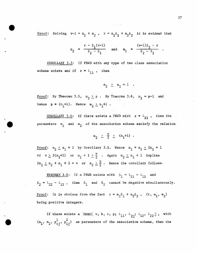
Proof: Solving v-1 = n1 + n2

, r = n1B1 + n2B2 it is evident that

r - 13 (v-1) (v-1) 13 - r1 and 2n2 = n1 =13 2 - 13 1 13 2 - 13 1

COROLLARY 3.3: If PBWD with any type of two class association

scheme exists and if r = All' then

37

>

Proof: By Theorem 3.5, n2~ p. By Theorem 3.6, n1 = p-1 and

hence p = (nl +1). Hence n2~ nl+l •

COROLLARY 3.4: If there exists a PBWD with r = All' then the

parameters and of the association scheme satisfy the relation

>v- >2

Proof: n2 ~ n1 + 1 by Corollary 3.1. Hence nl + n2 ~ 2n1 + 1

or or n1

+ 1 < v-2 implies

Hence the corollary follows.

THEOREM 3.9: If a PBWD exists with 13 1 = A2l - All and

13 2 = A22 - A12 • then 13 1 and 13 2 cannot be riegative simultaneously.

being positive integers.

with

1 2(n1 , n2 , Pij' Pij) as parameters of the association scheme, then the

38

parameters n1 , n2 can be expressed in terms of r, p, All' A21 , A12 ,

A22 as follows:

1 _ {A22 (-SlP + A21)r}n1 = A

21[rp D. .] and

provided A21 ~O and D. ~ 0 ,

Proof: We know that

2pb' = vr

By eliminating n1 from (1) and (3), we have

__(1)

__CD

=

Substituting this in (2),

r[A11P - A21 (P-1)]

A11A22-A21A12=

which proves the result.

1= -[rp­

A21

CHAPTER ·IV

PARTIAL DIFFERENCE SETS AND PARTIALLY BALANCED WEIGHING DESIGNS

4.1. Introduction.

A perfect difference set with parameters v, k, A, or in other words

a (v, k, A) -difference set, is a k-set - {dl

, d2

, .•. , dk } of integers

modulo v such that every a t 0 (mod v) can be expressed in exactly

A ways in the form

d.~

dj

- a (mod v) where d., d. ED.:l- J

The classical papers on difference sets include Singer [46] and

Hall [26]. A general survey of the subject is given by ~. Hall, Jr.

[26], and H.B. Mann [32]. A more comprehensive account of the present

status of "Difference Sets" can be found in [27]. The extension

of the idea of difference sets lead to (v, k,A) -group difference sets.

A perfect difference set with A = 1 leads to a projective plane,

called cyclic projective plane. For that reason, this type of difference

sets are called "projective difference sets" or "cyclic difference sets".

It has been conjectured that for a projective difference set,

n = (k-A) = (k-l) must be a prime power and this has been verified up

to n = 1600 [30]. All cyclic difference sets with k < 50 are now

known [26, 31, 40, 46].

There are two directions of research on difference sets: (i) construction

of new difference sets, and (ii) proo~ of impossibility of solutions for

certain parameter combinations. While the progress in the constructions

was comparatively slow, an impressive number of theorems ruling out many

classes of parameter combinations have been obtained in recent years.

40

It is known that Difference Sets give rise to a class of Balanced

Incomplete Block Designs [7, 27]. The incidence matrix of a BIB design

with parameters [4N-1, 2N-1, N-1] can be used to construct Hadamard

matrices of order 4N. Other Hadamard matrices may be obtained from

BIB designs with parameters (4N2 , 2N2

-N, N2

_N) . Hadamard matrices

have been used in the construction of binary codes [37]. The incidence

matrices of finite projective planes, finite Euclidean planes, and balanced

incomplete block designs are also being used in the construction of

error correcting codes. For a brief account of these applications one

can refer to I.M. Chakravarti [19]. These are Some of the considerations

which have led to the generalization of "perfect difference sets" to

"partial differece sets", which are the main concern of this chapter.

PARTIAL DIFFERENCE SETS:

Definition: Let v be a positive integer and let (d1

, d2 , "', dn )1

be a set of n l integers satisfying the conditions:

(i) the d's are all different, and o < d. < v (j=l, 2, ... , nl

)J

(ii) among the nl(nl-l) differences d.-d. , , (j , j' = 1, 2, ... , n1

,J J

jofj') reduced (mod v) each of the numbers occurs

g times, whereas each of the numbers el

, e2 , ... , en occurs h times,2

where {dl

, d2 , ... , dn e1

, e2

, ... , en} is a permutation of the1 2

set of integers {l, 2, ... , (v-1) } and g of h .The set of integers (dr' d2 , "', dn ) satisfying (i) and (ii)

1is called a partial difference set and is denoted by (v,n

1,n

2,g,h) -difference

set. Though the words"Partia1 Difference Sets"we"re not used, they

were applied in the construction of designs as early as in 1939,

41

by Bose and Nair [14], and a more precise formulation of this application

was given by Bose and Shimamoto [15].

The investigations on the methods of construction of weighing designs,

using the partial difference sets, are postponed until Section 4.4,

whereas the general description of the methods of construction of partial

difference sets and the other applications of the same are given

respectively in 4.3 and 4.5.

4.2. Perfect Difference Sets.

The following theorem concerning perfect difference sets throws some

more light on the existing families of difference sets formed with all the

quadratic residues. It is very useful in certain types of constructions

of the partially balanced weighing designs.

THEOREM 4. 2 . 1 : Let v = 4u + 1 be the power np of an odd prime,

be a primitive root of the Galois field

difference set, thenforms a (4u+l, u, A)

Then if

difference set.

nGF(p ) •

(4u+l, u, A)also forms a4u-2x }, ""

, ... ,6 10x , x

8 12x , x

Let xp •

4{x ,

2{x ,

Proof: Any non-zero element of will be of the form tx

where t = 0,1,2, or 3 (mod 4) •

(i) So starting with the case t = 0 (mod 4) , let x4h be

a fixed element ofnGF(p ) • Evidently,

=

{ () X4h __ (x4q+2 _ x4w+2)}the number of pairs q, w such that

{the number of pairs (q', WI) such that x4h+2 = (x4q ' _ x4w ')}

= A

42

if we assume that the original difference set (by hypothesis) is a

(4u + 1, u, A) -difference set. (Note: (q', w') = (q+l, w+l)) .

Similarly starting with the following type of elements, we conclude

as follows:

=

X4h+l __ (x4q+2_x4w+2)}(ii) {the number of pairs (q, w) such that

{ h b f . (' ') h h x4h+3 = (x4q '_x4w ')} --t e num er 0 pa~rs q, w suc t at A •

(iii) {the number of pairs (q, w) such that 4h+Z (x4q+2_x4w+2)}x =

{the number of pairs (q' , w') such that 4h+4 (x4q '_x4w ')} A= x = = ,

with the same notation of (q', w') .

'(iv) {the number of pairs (q, w) such that x4h+3 = (x4q+2-x4w+Z)}

~ {the number of pairs (q', w') such that x4(h+l)+1= (x4q'~x4w')} = A .

The conclusions (i) - (iv) establish that each of the non-zero

elements of GF(pn) occurs the same number of times in the set of

differences formed from 2 6 4u-2{x , x , ... , x }. Hence the theorem follows.

COROLLARY 4.Z.l: In case 48 >

{x , x , ••• , is a (4u+1, u, A)

-difference set, A is given by (u-l)4

Proof: The obvious relation u(u-l) = 4uA gives A = (u-l)4

COROLLARY 4.2.2: If p

where h ~ 1 (mod 2) , then

difference set with (p, hZ,

is an odd prime of the form 4hZ + 1 ,

2 6 10 4hZ-Z{x , x , x , ••. , x } forms a perfect

hZ-I-4-) as parameters.

Proof: By Theorem 8.6 of Mann [31] the 4-th powers form a perfect

difference set, when p = 4hZ + 1 is a prime and h ~ 1 (mod Z) •

43

Hence the corollary follows from the Theorem 4.2.1.

Note: this will be used in the construction of partially balanced weighing

designs (in Section 4.4) under the category "Rule II" •

4.3. Partial Difference Sets and their construction.

4.3.1. Partial difference sets:

Although no method of construction was given, few examples of partial

difference sets were given by Bose and Nair [14] and Bose and Shimamoto [15],

in constructing association schemes in partially balanced incomplete

block designs.

A lemma established by Nandi and Adhikary [35] can be restated

as follows:

LEMMA 4.3.1 (Nandi and Adhikary): (dl , d2 , "" dn ) is a partial1

difference set if and only if (d l ,d2 ,···,dnl) = (-d1 ,-42 , ... ,-dnl

),

where the n1 -sets are unordered sets.

Next, the following is an obvious necessary condition for the

existence of a (v, nl , n2 , g, h) -difference set.

LEMMA 4!3!2: A necessary condition for the existence of a

(v, nl , n2 , g, h) -difference set is that

=

In the next sub-section, some theorems are developed to construct

new series of partial difference sets, together with those which are

used for the constructions of the partially balanced weighing designs.

44

4.3.2. Some useful results for constructions of

Partially Balanced Weighing Designs:

THEOREM 4.3.1: Let n4u + 1 = P , where p is an odd prime and

n is a positive integer. Let x be a primitive root of nGF(p ) .

Then the 2u -elements 2 4 6 4u{x , x , x , .•• , x } constitute a partial

difference set {4u + 1, 2u, 2u, u-1, u} •

Remark: It can be seen that this theorem is valid for any u.

Proof: The proof of this theorem depends upon a lemma given in Bose

[ [7], Corollary 1.1.1] and which is stated below.

p is an odd prime, then among the elements

(xs - 1_1) there is one zero, (t-1) Q.R; 's ifand: t :7.non Q. R. i S

nis a primitive element of GF(p) , and if

2 4 6 s-3(x -1) ,(x -1), (x -1), ..• (x -1) ,

xIfLEMMA 4.3.3:

s = 4t+1 and one zero, (t-1) Q.R. 's and (t-1) -non Q.R. 's if

s = (4t-1), where QR and non-QR stand for quadratic residue and nonquadratic residul

can be written in the form of anformed from

Proof of the main theorem: The 2u(2u-1) differences which can be

2 4 6 4u{x , x , x , ••. , x }

array given below:

2 2x (x -1),

4 2x (x -1),

6 2x (x -1),

2 4x (x -1),

4 4x (x -1),

6 4x (x -1),

x 2(x4u- 2_1)

x\x4u- 2_1)

x6(x4u- 2_1)

4u( 2_1) 4u( 4_1) 4u( 4u-2_1)x x ,x x , •.. x x

__(1)

45

Evidently, each column of the array in (1) contains all even powers

of the primitive root x. Hence if (x2h_1) is an even power of x or

in other words a quadratic residue, then that entire column exhausts

the even powers. Similarly, if (x2h_1) is a non-Q.R., then that entire

h-th column exhausts the set of all odd powers, 'of x. So the frequencies

of the sets 2 4 6 4u 3 4u-1{x , x , x , "', x } and {x, x , .•. , x } are the

set,

same as the number of Q.R. 's and non-Q.R. 's among the set

2 4 4u-2{(x -1), (x -1), "', (x -1)}. But by the lemma, these are

respectively (u-1) and u. So by definition of the partial difference

2 4 6 4u{x , x , x , ..• , x } forms a partial difference set with parameters

(4u+1, 2u, 2u, u-1, u) , which proves the theorem.

Example 4.3.1: Let u = 3. Hence (4u+1) (=13) is a prime power.

We know that 2 is a primitive root of GF(13). It can be easily

verified that among the differences which can be formed from

(22,24,26,28,21°,212) = (4, 3, 12,9,10,1) , the set

(4, 3, 12, 9, 10, 1) occurs 2 times and each of the other remaining

6 non-zero integers (mod 13) , ocurs-3 times.

Example 4.3.2: Let u = 4 Hence (4u+1))=17) is a prime power. We

know that 3 is a primitive element of GF(17) and that

(1, 2, 4, 8, 9, 13, 15, 16) is the set of quadratic residues.

It can be easily verified that the frequencies are 3 and 4 respectively

for~.thesets of Q.R. 's and non-Q.R. 's among the differences formed from

(1, 2, 4, 8, 9, 13, 15, 16) •

46

Example 4.3.3: Let u = 9. Hence (4u+1) (=37) is a prime power.

We know that 2 is a primitive element of GF(37) It can be verified

that the frequencies of Q.R. 's and non-Q.R. 's among the differences

formed from the Q.R. 's [1, 3, 4, 7, 9, 10, 11, 12, 16, 21, 25, 26,

27, 28, 30, 33, 34, 36] are 8 and 9 respectively.

Example 4.3.4: Let u = 7 . Hence (4u+1) (=29) is a prime power •

We know that 2 is a primitive root of GF(29) It can be verified

that the frequencies of Q.R. 's and non-Q.R. 's among the differences

fromed from the quadratic residues (4, 16, 6, 24, 9, 7, 28, 25, 13, 23,

5, 20, 22, 1) , are 6 and 7 respectively.

The following theorem due to Mesner [ L33], page 16] is going to be

used to infer that 2 4 6 4u{x , x , x , "" x } of GF(4u+1) with primitive

root x defines an association scheme.

Mesner's Theorem: In a finite field of order v with additive

group G and multiplicative group G' , let m be a divisor of the

order (v-1) of G' such that N = (v-1)jm is even if v is odd,

and let s be a generator of G' • Let aO

= {O} , let be the

Definewhich containsbe the co-set ofa. , i=1,2, ..• ,m,J.

multiplicative sub-group of order N generated by sm, and let

i-lS •

an association relation F(v, m) in which two elements x, y of G

are i-th associates if and only if y-x to a. , i=O, 1 , 2 , ... ,m •J.

Then

for i, j, k in the range 1, "" m and interpreted

modulo m where necessary, F(v, m) is an m -class partially balanced

association scheme with parameters i= Pj+l,k+l

1= Pj-i+l,k-i+l'

and is equal to the number of elements of 0'. ••+1J-1.which occur

47

in the set obtained by adding the unit element 1 to each element of

The following is a corollary of the above theorem wli.icn defines

an association scheme, with respect to which partially balanced

weighing designs are constructed in Section 4.4.

COROLLARY 4.3.1: Let x be the primitive root of the Galois

field GF(4u+1) , where 4u+1 is the power of an odd prime. Let

AO

= {OJ • Let 2 4 4uA

l= {x , x , "" x } and 3 5 4u-1

A2

= {x, x , x , ••• , x }.

Define an association relation F(4u +1, 2) in which two non-zero

elements x and y are i-th associates if and only if y - X E A. ,1.

i=O,1,2. Then F(4u + 1, 2) is a 2-class partially balanced association

scheme with parameters v = 4u + 1, n1 = n2 = 2u and

F,1 = (:-1 :) P'2 (: :-~Proof: The proof follows from the above theorem, by taking

v = 4u + 1 and m = 2 .

Now we proceed to develop some results relevant for the construction

of the partially balanced weighing designs, which are dealt in [4.4].

LEMMA 4.3.6:

(i) Let v = 4u+1 be of the form of np p being an odd prime.

Then

(ii)

(iii)

qwx

Let x be a primitive root of GF nP'

4w qLet qw be defined by (x -1) = x w , for w = 1,2, ... , (u-l) •

4w+2u+qa hx were a = u-w .

Proof: Since x is a primitive element of GF(4u + 1) , x4u = 1 or

48

4u ux - 1 = a or y - 1 = a , where 4y = x Since 4

y = x :f 1 ,

except for the trivial case v = 5 ,

uy - 1 = a implies

u-1 u-2y + Y +. .. + Y + 1 = a or

x4 (u-1) + x4 (u-2) + ... + x4 + 1 = a __(4)

(x4W - 1) =

by the use of (4).

_ (x4_1) [x4 (u-1) 4(u-2) 4w+x + ... +x]

(x4w _ 1) = _ 4w( 4_1)[ 4(u-l-w) + 4(u-2-w) +x x x x ... + 1] •

Noting that the product of the last two expressions is [x4(u-w)_1]

and using the fact that x2u = -1, we have x4w_l = x4w+2u[x4(u-w)_1]

= 4w+2u+qax • This proves the lemma.

LEMMA 4.3.7: With the same notation and conditions «i) - (iii»

of the previous lemma, let u be ,of the form (4t ± 3) and let for

a fixed w, the sets {xqw+4

, xqw+8, "', xqw+4u} and

{ Qw-(2u+4w)+4 Qw-(2u+4w)+8 Qw-(2u+4w)+4u} be denotedx , x , .~e, X

respectively.by

and are disjoint (i.e. ) (empty set) .

are not disjoint, let there exist two integersProof:

rand

If

n n .s. u) such that Qw-(2u+4w)+4nx .

49

This implies that (4r + 4w - 4n) + 2u = 0 (mod 4u) .

Since 4 must divide the left hand side of the above congruence, 4 divides

2u. This is a contradiction, since u is of the form (4t + 3) . This

contradiction is due to the assumption that one member of sl is

identical with an element of s2'

s2 are disjoint.

Hence it follows that and

LElv1MA 4. 3 •8 : With the same notation as in the above lemmas,

and under the situation, where n is of the form (4u + 1) ,same v = p

let us put an additional restriction that u is of the form (4t + 3) .Then the number of Q.R. 's among the set of (u-l) -elements

{x4w_l, w=1,2, ..• ,(u-l)}

the same set.

is different from that of non-Q.R. 's among

Proof: Suppose if possible that the two numbers are the same. In that

h b (u-2l) . Al . f f 1 2 (1)case, t e num er is so 1 q = q or any w= , "'" u-u-w w

then (u-w) = w or u = 2w which is a contradiction to the assumption

that u = (4t + 3) . Hence it follows that qu-w and qw are distinct

for any fixed w , (w = 1, 2, ... , (u-l» . The conclusion

xqw = x4w+2u+qa , of the Lemma 4.3.6 can be written as:

qw - 4w + 2u + qa (mod 4u)

or qw - 4w + 2u + qu-w (mod 4u) (2)

(Le •. ) qu':"w - q - 4w 2u (mod 4u)w

- qw + 2u + 4(u-w) (mod 4u)

e - qw + 2u + 4a (mod 4u) (3)

It is obvious from (2) (or (3)) that if q is odd. thenu-w '

50

is also odd and vice versa.

is also even and vice versa.

Similarly, if is even, then

So the odd (even) powers of x, if at all there are any, among

{x4w_l, w=1,2, ... ,(u-l)}, can be paired, and hence the number

of odd (even) powers of x among this set must be of the form 2~ ,

for some suitable ~. But by a remark given in the beginning of the

proof, the common frequency of odd or even powers of x among

w=1,2, ..• ,(u-l)} is (u-1)2 Hence u-l-Z- = 2~

or u = 4~ + 1 which is a contradiction, since u = (4t + 3)

by condition (1) . This contradiction is due to our assumption that

the numbers of Q.R. 's and non-Q.R. 's are the same among the set under

consideration. Hence the lemma follows.

Remarks: The Lemmas 4.3.6 - 4.3.8 are developed to prove a

theorem, viz 4.3.2 which is useful for the construction of PBWD's.

THEOREM 4.3.2:

(i) Let p be an odd prime and let v be an integer of the

form 4u + 1, which can be expressed as nv = p

(ii) Let u be of the form (4t + 3) •

4{x ,

(iii) Let x be a primitive root of GF and let the 4 setspn

8 4u} 2 6 10 4u-2 5 9 4 (u-l)+lx , ..• x , {x, x , x .•. x }, {x, x , x , ... x }

~d3 7 11{x , x x 4u-1x } be denoted by A1 , A2 , A3, A4

respectively.

(iv) Among the (u-1) distinct elements

{x4w _ 1, w = 1, 2, ... , (u-l)}, let there be g quadratic residues.

51

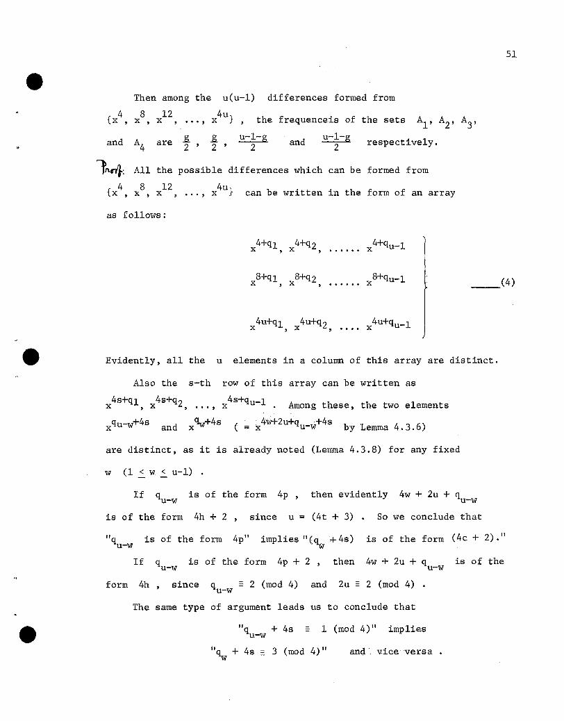
Then among the u(u-l) differences formed from

{x4 8 12 x4u} the frequenceis of the sets AI' A2 , A3

,, x , x , ... ,

and A4are .B. .B. u-l-g and u-l-g respectively.2

, 2 , 2 2

lnrlj.: All the possible differences which can be formed from

{x4 8 12 x4u } can be written in the form of an array, x , x , ... ,

as follows:

4+ql 4+q2 4+qu-lx , x " • • . •. x

8+qu-lx __(4)

4u+ql 4u+q2 4u+qu-lx , x , •••• x

Evidently, all the u elements in a column of this array are distinct.

Also the s-th row of this array can be written as

4s+ql x4s+q2 4s+qu-l Among these, the two elementsx , , ..., x .qu-w+4s and

qw+4s ( . 4w+2u+q w+4s by Lemma 4.3.6)x x = x u-

are distinct, as it is already noted (Lemma 4.3.8) for any fixed

w (1 ~ w ~ u-l) •

If is of the form 4p , then evidently 4w + 2u + qu-w

is of the form 4h + 2 since u = (4t + 3) So we conclude that

"q is of the form 4p" implies "(~ + 4s) is of the form (4c + 2). "u-w

If qu-w is of the form 4p + 2 , then 4w + 2u + qu-w is of the

form 4h since q = 2 (mod 4) and 2u = 2 (mod 4)u-w

The same type of argument leads us to conclude that

"q + 4su-w1 (mod 4)" implies

ilq + 4s = 3 (mod 4)"w

and vice versa .

52

So for a fixed s, the elements can be paired as

( 4s+qu-w 4s+qw)x , x for different w's such that this unordered pair will

be of the form (x4c+l , x4b+3) or

This assertion is true for all s (s = 1,2, "" u). This together

with the fact that each column exhausts all the possible 4-th powers

(which are u in number), when xqj is taken out as common factor,

for j = 1, 2, "" u, lead to the conclusion that the columns

of the array (4) can be so paired that u + u = 2u individual

elements of each pair of columns exhaust all the Q.R. 's exclusively

or they exhaust all the non-Q.R. 'so

So if g and h stand for the Q.R. 's and non-Q.R. 's among

{x4w_1, w=1,2, ... ,(u-l)} , we conclude the following:

(i) h = u - 1 - g •

(ii) g ~ h (by Lemma 4.3.8) .

(iii) The number of elements of the form tx among

those of the array (4) is £2 ' or (u-l-g)

2 according as

t is even or odd.

where

(iv) All the u elements in a column of the array (4) are

txdistinct and each column contains elements of the form

t covers exclusively all possible elements of the form t - i (mod 4)

for some i (i = 0, 1, 2, or 3) .

So with the help:oLarray (4)" it follows that among the u(u-l)

53

the frequenciesdifferences formed from Al = {x4 8 x4u}, x , ... , ,

of the sets AI' A2 , A3

, A4 are .8- .8. u-l-g

2 , 2 ,2

respectively. This proves Theorem 4.3.2.

and u-l-g2

COROLLARY 4.3.2: With the same notation as in Theorem 4.2.2,

among the differences formed from 2 6x , x , ... , 4u-2x

the frequencies of AI' A2 , A3

, A4u-l-g .- 2 ,respect~vely.

are .8-2 '

.8.2 '

u-l-g2

and

248or .x {x , x ,

2 6 4u-2. 2 4u 4 8 4u-4A2 = {x , x , "', x } = x {x ,x, x , ... , x }Proof: Since

... , 4u-4 4u}x ,x , we get the same type of differences

as in the theorem (for the case AI)' except for the fact that each

t 2resulting x will be multiplied by x

So denoting the set of differences for Al and AZ as Df and

D respectively, the assertion of the Theorem 4.3.2 thats

implies

u-l-g+ 2 A3

u-l-g+ 2 A4

Ds

+ .8. A + u-l-g A2 1 .. 2 4

u-l-g+ 2 A3

(by the remark of the above paragraph).

Hence the corollary follows.

4.4.

54

The construction of PBWD's from difference sets.

be a partial difference set with parametersLet {d1 , d2 ,

(v, n1 , n2 , ~, S)

"" d }n1

and let D = {d1

, d2 , "" and

define a cyclic association scheme.

Suppose {a'l' a'2' ... , a, } and {b'l' b'2' .•• ,'b,} (i=1,2, ... ,t)1 1 1p 1 1 1p

are 2t -sets of distinct integers, each of size p , with the following

properties:

I.

disjoint.

are

(i=1,2, ... ,t, j:f iI., = 1,2, •.. ,p), each

II. Among the differences (a., ­1J

a , n ), (b" - b. n )1", 1J 1",

dj occurs All times.

III. Among the differences mentioned in II, each eq

(q=1,2, ... ,n2)

occurs A12 times.

IV. Among the differences of the form + (a., - b, ) ,1J 1i1.,

each d,J

occurs A21 times.

V. Among the differences mentioned in IV, each eil., (iI.,=1,2, ..• ,n2)

occurs A22

times.

We treat the initial block {a· 1 , a· 2 , "" a. ; ~'1' b'2'1 1 1p 1 1

of the i-th set as 'O'-th block of that set and the block

... , b, }1p

where each{ail + j, ai2 + j, ... , aip + J; bi1 + j, ... , b ip + j}

element must be interpreted as belonging to the residue system mod v, is

called j-th block generated from the initial block. Wnen we consider the

residue '0', it will be taken as v. With this notation, we can state

and prove the following theorem:

55

THEOREM 4.4.1: If the 2t sets {ail' ai2 , ... , a. } ,~p

i=1,2, ... ,t, satisfying the properties I - V{b· 1 , b. 2 , "" b. }1. 1. lp

exist, then the vt blocks generated by developing the sets

{ail' a i2 , "" a. ; b. l , b. 2 , "" b. }~p ~ ~ ~p

treated as the initial blocks,

constitutes a partially balanced weighing design with the parameters:

__(1)

and with the association scheme defined by the partial difference set

... , with parameters:

n -n +13-12 I .

n -13I

__(2)

/

n1-a-l'jn 2-n1+a+1 J

../".......

and 1\ = (

\~l-a-1

13

= ~~-aThus the corresponding association scheme called cyclic association

scheme is specified by the parameters a, S, n, and n2

Proof: For some verifications arising in the proof, ''Ie can have ,;\11 idea

of the situation by restricting to a single initial block from out of the

set of t -blocks.

We know that the number of blocks is vt when we start with t initial

blocks. We also know that p is the half-block size.

Next, consider a treatment numbered u. In the development of

{ail ' ai2 , ... , a. ; bil

, bi2 ' ... , b. }, u occurs in the block number~p l.p

q , if and only if we can find an a .. or b .. such that~J ~J

a .. + q = u or b .. + q = u . So q can be uniquely fixed by~J 1.J

56

q = u - aij or u - b ij as the case may be. So restricting to the

blocks generated from {ail' a i2 , ... , a ip ; bil' b i2' ... , b ip} ,

the blocks in which u occurs are the ones numbered u - ail' u - ai2 \ •..

u - aip ' u - bi!' u - b i2l...u - b. As there are t 'initial blocks,l.p

r = 2pt .Let u and s be two treatments, which are first associates.

Then the q-th block of the i-th set will contain both u and s in

the first half-block if and only if we can find two integers a .. and1.J

aiQ, such that

a .. + q = Ul.J

__(3)

= s __(4)

hypothesis be denoted by D.

mentioned in the

- s .aij - aiQ, = u

Let the partial difference set

From (3) and (4)

If u and s are fixed, then (u - s) is also fixed and it is an

element of D since u and s are first associates of each other.

Thus (u - s) can be identified to be dh

(say). Then it is evident that

u and s occur together in the first half of the i-th set, as many times

as dh

can be represented as a difference between two a. 's •l.

Similar argument applies to the other half blocks of the i-th set

(b il , b i2 , "', b ip )' So the number of times dh occurs either as

difference between two a. 's or as difference between two b. 's ,l. l.

is the same as the number of times u and s occur together. But

57

this number is All by the condition II. Also this entire argument

is valud as long as the pair constitutes a pair of first associates.

In the same way, it is easily seen that two treatments which are

first associates will occur in opposite half blocks of the same block

A2l times and two treatments which are second associates will occur in

the same half block A12 times and in opposite half blocks of the same

block A22

times.

THEOREM 4.4.2: A ncessary set of conditions for the existence of

a cyclic PBWD described in Theorem 1 is that:

(i)

(ii)

Proof:

=

=

2tp(p - 1)

22tp

(i) The totality of pairs which can be formed from a single initial

block is p(p-l) and hence the total number of all possible pairs both

of whose elements belong to the same half block, is 2tp(p-l) . Considering

any pair is equivalent to considering the difference between the two integers

The

representing the pair of treatments.

belong to D = {dl

, d2

, ... , dnl

} or

existence of the PBWD guarantees that

But difference between any pair must

E = {aI' e2 , ... , en2

}·

each element of D occurs as

a difference between the elements of such pairs All times and that each

element of E occurs A12 times.

Since there are

it follows that:

elements in D and

=

elements in

2tp(p-l)

E ,

This proves (i). Similar argument establishes (ii).

THEOREM 4.4.3: Let p be an odd prime and let

58

nv = p be of the

form (4u+l) Let 4 8 4uAl = {x , x , "" x } 2

= {x , 6x , 4u-2x }

where x

Let

4 4u-2x -x

is a primitive element of GF(pn) •

2(AI - A2) stand for the u differences

8 2 8 6 8 4u-2 4u 2x -x , x -x , .•. , x -x •.• , x -x,

4 2 4 6(x -x , x -x ,

4u 6 4u 4u-2)x -x, ..• , x -x

Similarly, let (A2 - AI) be defined.

(i) Let u be of the form (4t+3) and

Let there be g -quadratic residues among the (u-l) -elements

h=1,2, ... ,(u-l) then among the 2u2 -differences formed

from (AI - A2) and (A2 - AI) , each quadratic residue occurs

(u-l-g) times and each non Q.R. occurs (g+l) times.

Proof: The set (AI - A2) of differences can be written as an array given

below:

2 4u-2......... x (x -1)

6 4u-2......... x (x -1)

will be of the form'f f

h + 48 + 2 = R whichw w

4u-2( 2_1') 4u-2( 6_1) 4u-2( 10_1) 4u~2( 4u-2_l )x x , x x , x x , •••••.. x x .

So any arbitrary element of (AI - A2)

xhw+4s+2 where (x4w+2_l) = xhw Let

obviously depends on the arbitrary integer s. With this notation

hw+4s+2 Rwx = x

The corresponding element (i.e. just the negative of this arbitrary

R Rw+2uelement) of (A2 - AI) can be written as (-l)x-~ = x since it

f 11 f h d f ' " f x that x2u -- (-1).o ows rom tee 1n1t10n 0 Since

leads us to the conclusion that

2u = 2(4t+3) = 4(2t+1) + 2 ,

l\v Rw+2uin x and x

(mod 4) according as

the <co.mparisoill of Rw

and

59

R +2u appearingw

R +2u - 0, 1, 2, 3w

Rw

2, 3, 0, 1 (mod 4) __(5)

Let us write the u elements of the (w+l) -th column of the above array

and the u -elements corresponding to their negatives as a partitioned

row vector as follows:

( 2+hw 6+hw 4u-2+hwI 2+hw+2u 6+hw+2ti .4u-2+hw+2u) (6)1x ,x , ... x x ,x , ... x .

Now let us: s.t,uC!W the nature of these elements. Let (h +4s+2)w

and

(h +4c+2+2u) be two arbitrary elements of this partitioned row vector takenw

respectively from the first and second part. Comparing these two elements,

it is obvious that if h +4s+2 = h +4c+2+2u (mod 4u), we have to concludew w

that 4(s-c) = 2u(mod 4u) and hence that 4 divides 2u, which is

impossible.

Also, it is obvious that the first part of (6) is a set of u

distinct elements and that the second part of (6) is a set of u distinct

elements.

So it follows from (5) that all the 2u -distinct elements of (6)

are quadratic residues or non-quadratic residues according as the corresponding

xRw (see (5» is a quadratic residue or a non-residue, respectively.

So if the array (A2A

l) is formed directly from (A

l- A

2) by

change of sign of each element, we have the conclusion that:

e (i) the (w+l) -th column of the combined array. Al-A2

. eitherA2-Al

exhausts all the 2u Q. R. 's or all the non-Q.R. 'so

60

(ii) If c is the number of quadratic residues among

2 6 4u-2{(x -1), (x -1), ... , (x -I)}, (i) implies that the set of

quadratic residues repeats itself c times in the combined array.

Determination of c: By the Corollary (1.1.1) of [3] there are (u-l)

, 2 4 6 4u-2Q.R. s among {x -1, x -1, x-I, ... , x -I} and hence by the notation

of g in the hypothesis, c = u-l-g .

So by (i), each quadratic residue occurs (1l-1-g) times in

Since the total number of rows is'A '-A )l 1 2A2-Al

non Q.R. occurs among (AI -A2 )A

2-A

lThis proves Theorem 4.4.3.

g + 1

u

( =

in this array, each

u-(u-l-g» times.

THEOREM 4.4.4: Let p be an odd prime and let nv = p of the

form (4u + 1) . Let x be a primitive root of nGF(p ) •

(i) Let· u be of the form (4t + 3) .

(ii) Let there be g quadratic residues among the (u-l) -elements

{(x4h_l), h=1,2, ... ,(u-l)}.

Then the initial block 4 8{x , x , ... , 4u

x2x , 6x , 4u-2

•• " x }

when developed, gives a partially balanced weighing design with the association

scheme defined in the Corollary 4.3.1 and the parameters of the design

being (v, b, r, p) = (4u+l, 4u+1, 2u, u) and

Proof: We follow the notation of Al and A2 of the Theorem 4.4.3

and note that the initial block can be written as: {AI; A2} .

61

Step 1: By the Theorem 4.3.2, among the differences formed from Al '

each quadratic residue occurs ~ times and each non Q.R. occurs2

u-l-g2

times.

Step 2: By the Corollary 4.3.2, among the differences formed from

each Q.R. occurs 1 times and each non Q.R. occurs u-l-g2

Step 3: By the Theorem 4.4.3, among the differences {AI - A2 , A2 - AI}

which are the opposite differences arising from (AI; Ai. each Q.R.

occurs (u-l-g) times and each non Q.R. occurs (g+l) times.

Steps 1 and 2 imply that among the differences formed from the same

half block, each Q.R. occurs g times and each non Q.R. occurs

(u-l-g) times. Hence (All' A12) = (g, u-l-g) .

Step 3 implies that (A 2l ,A22 ) = (u-l-g, g+l) . Hence the initial

block under consideration satisfies all the 5 conditions of the Theorem

2 4 6 4u4.4.1, with {dl , d2 , "" d2u} = {x , x , x , ..• , x } and

3 5 4u-l{el , e 2 , "', e2J = {x, x , x , "', x } defining the

association scheme.

The parameter sets (1) and (2) of the Theorem 4.4.1 are given by:

= (4u+l, 4u+l, 2u, u; g, u-l-g, u-l-g, g+l)

and = = 2u , and P 2 =(

u u "'\

u U-l) ,as noted in the Corollary 4.3.1.

62

EXAMPLE 1: u = 3; v = 4 x 3 + 1 = 13 2 is a primitive root of

GF(13) (2 4 , 28 212) = (3, 9, 1) (22, 26 210) = (4, 12, 10), ,

(24_1, 28_1) = (2, 23) .g = °. .. .

By Corollary 4.3.1 (4, 3, 12, 9, 1O, 1) defines a cyclic

association scheme and by Theorem 4.4.4, (3, 9, 1; 4, 12, 10) gives

a PBWD with the parameters of the association scheme and the design

being given by (using (8) and (9»

= (6, 6)

(13,13,6,3;0,2,2,1)

__(9)

This can be seen by the direct verification.

EXAMPLE 2: u = 7; v = 4 x 7 + 1 = 29. 2 is a primitive root of

GF(29) and

(16, 24, 7, 25, 23, 20, 1)

g = 4 .

By the Corollary 4.3.1, (4, 16, 6, 24, 9, 7, 28, 25, 13, 23, 5, 20, 22, 1)

defines a cyclic association scheme and by Theorem 4.4.4

(16,24,7,25,23,20,1; 4, 6, 9, 28, 13, 5,22) gives a PBWD with the

63

parameters of the association scheme and the design being given by

(using (8) and (9»

;)(v, b, r, p; All' A21 , A12 , A22) = (29,29,14,7; 4,2,2,5) .

This is verified separately by the direct method.

EXAMPLE 3: u = 15, v = 4 ~ 15 + 1 = 61. 2 is a primitive root of

GF(61) h {x4w} ,T e powers and {(x4w_1), w=1,2, ... ,14}

can be seen to be {16,12,9,22,47,20,15,57,58,13,25,34,56,42,1} ,

{4,3,48,36,27,5,19,.60,45,49,52,39,14,41,46} and

(228,215,23,255,258,226,25°,252,232,28,29,221,237,254) respectively.

So evidently g = 8. So the parameter sets of the corresponding

association scheme and the PBWD are given by:

= (30, 30) =(14 15)15 15

= f5 15)~5 14

and (v, b, r, p; All' A21 , A12 , A22 ) = (61,61,30,15;8,6,6,9) .

THEOREM 4.4.5: Let v = 4u+1 be the power np of an odd prime, p .

4 8 4u}If Ix , x , "" x forms a perfect difference set, then

4 8{x , x , ... , 4u

x2x , 6 10 4u-2

x , x , "" x } generates a PBWD, with

2 4 6 4u•• " d2u } = {x , x , x , "" x } defining the cyclic

association scheme and with the following paramter sets of the association

scheme and the design:

64

Zu , PZ =

u-1 u-1 u-1 u+1(v, b, r, p; All' AZl ' AlZ ' AZZ ) = (4u+1,4u+l,Zu,u;--Z-'--Z-'--Z-'--Z-)

form a. partialBy Theorem 4.3.1, the elements

Proof: By Theorem 4.Z.1, both half blocks of the initial block are

u-l (u-l u-1)difference sets, with A= --4- and hence (All' A2l ) = Z' Z .

Z 4 6 4u{x , x , x , "" x }

difference set with {4u+1, Zu, Zu, u-1, u} Hence among the opposite

differences arising from the initial block, each Q.R. occurs (u_1)_(u;1)=

(u-l) . u-1 u+l--Z- t1mes and each non Q.R. occurs u-(--Z-)=(--Z-) times. Hence by the

theorem (4.4.1) and the corollary (4.3.1), it follows that the initial

Z 4 4ublock generates a PBWD and that {x, x , "" x } defines the cyclic

association scheme. Hence the theorem follows.

COROLLARY 4.4.1 If v = 4u+1 is a prime, where u is of the form

(Z9-+1) Z 4then {x ,8

z , ... , 4ux

Z 6x , x

10x , ... , 4u-Z

x } generates

a PBWD with the same association scheme as in the Theorem (4.5.),

Proof: This fo11ws from the Theorem 4.4.5, using the result that under

the above circumstances, {x4 , x8 , "" x4u} forms a perfect difference set.

EXAMPLE 1: u = 9, v = 4 x 9 + 1 = 37. Z is a primitive root of

37.

4{(x, 8x , ... , 36 Z

x ), (x ,6

x ,34

• '" x )} can be written as

{16,34,Z6,33,10,lZ,7,1; 4,Z7,Z5,30,36,Zl,3,ll,Z8}

= 18 -(: :)

65

and (v, b, r, p; All' A2l , A12 , A22 ) = (37,37,18,9; 4,4; 4,5)

which is true by direct verification also.

Remarks: The Section 4.4 can be :concluded",asan ·attetnpt-:to:construct

partially balanced weighing designs, w:i.tPL:.cycliccassociatd:On;sc1;!.emes:, 'under

two different methods which form particular cases of two rules, mentioned

below as Rule I and Rule II.

Rule I:

1. Association scheme:

(a) G is a set of v elements c/,O {= e} ,

c/'l' c/'2' ..., c/'v_l .

e (b) G - {e} = El

u E2

(c) El forms a partial difference set.

2. Design:

(a) Dl and D2 are two disjoint sets, each containing

(b)

.. :p distinct elements from G

If D.D.-l stands for the set of all differences formed by~ J

and then

(c) =

Rule I says that if such a pair Dl , D2 can be found, then (Dl ; D2)

leads to a PBWD, provided (El ,E2) can be found with conditions described in 1.

Rule II:

1. Association scheme:

(a), (b), (c) are the same as in Rule I.

2. Design

(a) Dl and D2 are disjoint.

(b) Dl and D2 are perfect difference sets separately.

(c) IDII = ID2 1 .(d) {(](,l)El } u {(](,2)E2} = Dl u D2 ' with ](,1 :/: ](,2

Rule II says that if such a pair Dl , D2 can be found, (Dl ; D2)

leads to a PBWD, with the association scheme given by (El , E2) .

The parameter sets of the designs constructed under Rules I and II

can be described in Tables 4.1 and 4.2.

Both of the Tables 4.1 and 4.2 describe Some examples of partially

balanced weighing designs with cyclic association scheme. But they

describe constructions based on Rules I and II respectively. Tables

4.l(A) and 4.2(A) describe the parameter-sets for a few of the PBWD's

of this type, whereas 4.l(B) and 4.2(B) describe the actual plans of

such designs.

66

..

TABLE 4.1. (A)

S. No. v r p b .. n1 . u2 }\ll A21 , A A2212

4u+1 2u u 4u+1 2u 2u g u-1-g u-l-g g+1

1 13 6 3 13 6 6 0 2 2 1

2 29 14 7 29 14 14 4 2 2 5

3 61 30 15 61 30 30 8 6 6 9

eTABLE 4. 2. (A)

S. No. v r p b n1 n2 All A21 A12 A22

4x2+1 2x2 2 4x2+1 2x2 2x2 2 2 2 x2+1x -1 x -1 x -1x 2 2 -2- 2

1 37 18 9 37 18 18 4 4 4 5

2 101 50 25 101 50 iO 12 12 12 13

67

68

TABLE 4.1. (B)

All == 0, A21 == 2, A12 ==

/ ;) ;PI =~ E ==2

Association Scheme

6

Initial Block

(3,9,1; 4,12,10)

5,4,13,10,11,2

1st' Associate

v == 13, r == 6, p == 3, b == 13, nl == 6, n2

2, A22 == 1

~ ~)Variety

1

Design (1

Design (2 v == 29, r == 14, p == 7, b == 29, nl == 14, n2

14

A == 4,11

A == 2,21A12 = 2, ;\ == 5

22

6 77

7 76

Association Scheme

Variety 1st Associate

1 5,17,7,25,10,8,29,26,14,24,621,~23,2

Initial Block

16,24,7,25,23,20,1;4,6,9,28,13,5,22

Design (3 v == 61, r == 3O, p == 15, b == 61, n1 == 30, n2 == 30

A == 8, A == 6, 1\ == 6, ;\ 911 21 12 22

CS"

l' . (14 lS) £215 )==1 15 ' 14

Association Scheme

Variety

1

1st Associates

17,13,10,2~,48,21,16,58,59

14,26,35,57,43,2,5,4,49,37

28,6,20,61,46,50,53,40,15

42,47

Initial Block

16,12,9,22,47,20,15

57,58,13,25,34,56,42,1;4,3,48,36,27,5,19,60,

45,49,52,39,14,41,46

Design (4

TABLE :4 ~2 • (BY

v = 37, r = 18, p = 9, b = 37, nl = 18, n2 = 18

1\1 = 4, 1~1 = 4, ""12 = 4, ~2 = 5

69

Variety

1

Association Scheme

1st Associate

17,35,27,10,34,11,13,

8,2,5,28,26,31,37,22,

4,12,29

Initial Block

16.34,26,9,33,10,12,

7,1; 4,27,25,30,36,21

3,11,28

\

CHAPrER .V

CONSTRUcr ION OF PBWD WITH TWO ASSOCIATE CLASSES

5.1. Introduction

Partially Balanced Incomplete Block designs have been introduced by

Bose and Nair [14]. The classification of association schemes has been

explained in a paper by Bose and Shimamoto [15]. This classification

has been followed by Bose, Clatworthy and Shrikhande [12] and Clatworthy

[20] in preparing the tables of partially balanced designs with two

associate classes. As the cyclic type of association scheme has already

been defined and since the corresponding PBWD's have been constructed

in the previous chapter, this chapter deals with the construction of

PBWD's with an association scheme other than the cyclic one.

Before considering different association schemes, they are first

described below.

(a) Group divisible (GD) association scheme: In this case there

are mn treatments, which are divided into m groups of n treatments

each. Two treatments belonging to the same group are first associates,

and two treatments belonging to different groups are second associates.

The association scheme can be exhibited by writing down the mn treatments

in the form of a rectangular array, the treatments of the same group

occupying the same row. It is readily seen that the parameters of the

association scheme

Pl = c:z n(:-l~So obtained are v = ron, n

1= n-1, n

2= n(m-l),

and Pz = Cn:l) n::~::)It has been shown by Bose and Connor [13] that for a GD design,

Hence they have been divided into three classes:

71

(i) Singular (8) if r = Al ,

(ii) Semi-regular (SR) if r > Al and rk - A2v 0 ,

(iii) Regular (R) if r > Al and (rk - A.2v) > 0 .

The partially balanced weighing designs of the GD type are discussed

in Section 5.5.

(b) Triangular association scheme: We take an m x n square, and

fill in the m(m-l)2

positions above the leading diagonal by different

treatments, taken in any prder. The positions in the leading diagonal

are left blank, while the positions below;this diagonal are filled so

that the scheme is symmetrical with respect to the diagonal. Two treatments

in the same row (or same column) are first associates. Two treatments

which do not occur in the same row or same column are second associates.

It is readily verified that the parameters of the association scheme so

obtained are v = l1).(m-l)/2, nl = 2m-4, n2 = (m-2)(m-3) /2 ,

(-2 m-3 0Gm:a

2m-8PI and P

2 =m-3 (m-3~(m-4) (m-4) (m-5)

2

This scheme is called the triangular association scheme.

The PBWD's of the triangular type are constructed in Section 5.3.

(c) L2

-association scheme: Consider2

v = s treatments which

may be set forth in a s x s scheme as:

1

s+1

(s-l)s + 1

2 •••••••• s

s+2 ....•.. 2s

(s-1)s + 2 .•. s2

72

We define two treatments as first associates if they occur in the same.. ,

row or column of the square scheme, and second associates otherwise. The

L2 -association scheme.association scheme so defined may be called the

The of the L2 scheme 2parameters are v = s ,

(-2 8-1 )PI = and P

2=

s-l (s-l) (s-2)

nl = 2(s-1), n 2 =

0<8:2) :~:::~)

2(s-l)

The PBWD's with the L2 -type association scheme are constructed in

Section 5.4.

Before discussing the construction methods of PBWD's with different

association schemes, two general theorems (1 and 2) are proved in Section

(5.2) which enable us to obtain PBWD's from some existing PBWD's and

resolvable PBIB designs.

Lastly the parameter sets corresponding to the PBWD's (which are

constructed) with the (i) triangular association scheme (2) L2 ­

association scheme and (iii) GD -association scheme are tabulated in

Tables 5., ·6\ and (7A - ~") respectively.

5.2. Some general theorems.

THEOREM 5.1: If there exists a PBWD(v, b, r, 3; All' A21 ; A12 , A22 ) ,

we can deduce a PBWD(v, 9b, 6r, 2; 3All , 4A21 , 3A12 , 4A 22) .

Proof: Taking any specific block, we can form 9 blocks by taking all

possible pairs from each of its half blocks. Hence for the deduced design,

the number of blocks b* = 9b. To find r, it is evident that there

are two possible pairs containing a given object, which can be formed

73

for each of these possibilities. So whenever a fixed treatment occurs once

in the original design, it occurs 6 times in the deduced one. Hence the

number of replications r* = 6r. Whenever a pair is fixed in the deduced

design, it constitutes a half block three times for each original block

which contains the same. Hence the A -parameters Atl' At2 are given by

Similarly considering the blocks in which two treatments occur in

opposite half blocks, we have A~l = 4A2l , A~2 = 4A 22 • Hence the

theorem follows.

THEOREM 5.2: If there exists a resolvable PBIB design

[v, rt, r, k, Al , A2] with any association scheme and b = rt blocks,

then there exists a

Proof: Let us start with a set of t -blocks of the resolvable PBIB

design, which constitute a single replication. Let us form all possible

(~) pairs of blocks from out of these t blocks. Let us form a weighing

design by taking these (~) pairs as blocks 6f the former, one block of

each pair being the first half block and the other one as second half

block. In this way, it is evident that each "resolvable set" of the

given PBIB design gives rise to (~) blocks of the corresponding weighing

design. Hence where

(v*, b*, r*, p*; Atl' A~l; Ar2' A~2) are parameters of the weighing design.

If we fix a particular treatment 8 and consider "a resolvable

set of t blocks", it is evident that the corresponding blocks of the

weighing design contains this treatment (8), (t-l) times. But this

74

arbitrary treatment e occurs r times, occuring once in each of the

r sets. Hence r* = r(t-l) . Since evidently v* = v and p* = k ,

we have to verify the A -conditions to complete the theorem.

Since each block of the PBIB design appears (t-l) times as a half

block of the weighing design, the number of times any two first (or second)

associates occur together in the same half block is (t-l) multiplied

by the corresponding number Al (or AZ

) in the original PBIB design

(the half block being treated as a complete block).

Hence the number of times any two treatments occur together is

(t-I)AI or (t-I)A Z according as the two treatments are first or second

associates respectively. Hence Atl = (t-I)AI ' AtZ = (t-I)AZ .

To find the other parameters A~l and A~2' we note that there are

(r - AI) -"resolvable sets~' in which two "first associate"-treatments

e and ~ occur in different blocks rather than in the same block. By

this construction method of the weighing design, it is thus evident that

A~l = (r - AI)' Similar argument applies to two "second-associate"­

treatments, giving A~Z = r - AZ ' This completes the proof.

NOte: Although this theorem applies to any resolvable PBWD to be constructed,

it might not be economic to use the method proposed here, for the construction

of PBWD, in case t is very large. So it is wise to use this theorem

for constructions when t = Z. Most of the examples considered in

latter sections are cases where t = Z .

75

5.3. PBWD with triangular association scheme.

THEOREM 5.3: From a triangular association scheme with n(n-l)v = 2

treatments, with n even, we can construct a Partially Balanced Weighing

Design with the same association scheme and with parameters

= l·n(n-l)2 '

2(n-2)! n-l2

(n-3) ! (n-3)!0, ~

Proof: We know that there are (n-l) elements in each row, since

diagonal elements will be omitted. Suppose we construct from each row

all possible blocks formed by taking (n-l)2

objects in each half block.

As there are n rows

there are evidently

If we consider all possible partitions of the (n-l) elements of a row,

1:. [ (n-l)! ] distinct partitions.2 (n;l) ! (n;l) !

in the array for a traingular association scheme,

the number of distinct blocks which can be formed by this procedure is

Since by definition of this scheme, the array is symmetrical

about the principal diagonal, any element i appears twice, once in the

row in which i is present and secondly in the row corresponding

to the column in which i appears. By the procedure of constructing

the blocks, it is evident that for every row in which ." ,1 is present,

76

we can form

distinct possible blocks in which Ii' occurs in either half block.

Hence

r = [ -J2 (n-2)!

_ (n/) ! (n/)~

To determine All' we have to fix two first associates'1i:n'fo t'Ul:ing".;

all possible blocks, with these two lying in the same half block. So

out of (n - 1 - 2) = (n - 3) remaining objects, we have to put

( = n;5) in the half block with this fixed pair and remaining

in the second half block. As we can assume without loss of generality

that the two fixed treatments occur in the first half block, the number is

= (n-3)!

As there is only one row with a given fixed pair of numbers, All is

given by the above number.

The same type of argument applied for two first associates to

occur together in opposite half blocks gives the following:

=

By the method of construction of the half blocks and the blocks, any

two second associates can occur together neither in the same half block

nor in the opposite half blocks.

the theorem follows.

Hence A = 0 = A12 22

Hence

EXAMPLE 1: From the association scheme given on page 229 [12] with

n = 5 , we get a PBWD(10, 15, 6, 2; 1, 2; 0, 0) given as follows:

1,2; 3,4 2,5; 8,9 4,7; 9,10

1,3; 2,4 2,8; 5,9 4,9; 7,10

1,4; 2,3 2,9; 5,8 4,10; 7,9 .

1,5; 6,7 3,6; 8,10

1,6; 5,7 3,8; 6,10

1,7; 5,6 3,10; 6,8

The parameters of this design can be compared with those of the

BWD given by Bose and Cameron [see Design 13, page 158 of [10]].

The parameters of this BWD are given by

77

= (la, 45, 18, 2; 2, 4) .

EXAMPLE 2: The association scheme given in T31 of page 238 [12]

corresponds to n = 7 and by substitution of this value we get a

PBWD(21, 70, 20, 3; 4, 6; 0, 0) with the first 10 blocks (using the

first row of the scheme) given below:

1,2,3; 4,5,6

1,2,4; 3,5,6

1,2,6; 3,4,5

1,3,4; 2,5,6

1,3,5; 2,4,6

1,3,6; 2,4,5

1,4,5; 2~3,6

1,4,6; 2,3,5

1,5,6; 2,3,4

These parameters can be compared with those given by Bose and

Cameron in 2.3.1 of page 151 [10] by substituting t = 5 and hence with

those given by (v, b, r, p; AI' A2) = (21, 70, 20, 3; 2, 3) .Examples 3,4, 5 which are given below are obtained from T-3, T-16

and T -22 [12], by the subdivision of the blocks.

EXAMPLE 3: The plan of the PBWD[10, 15, 6, 2; 1, 2; 0, 0] obtained

from T-3 of page 230 [12], is given below:

Plan Association Scheme

1,2; 3,4 3,8; 8,10 x 1 2 3 4

5,6; 7,1 4,9; 7,10 1 x 5 6 7

8,9; 2,5 1,4; 2,3 2 5 x 8 9

10,3; 6,8 1,6; 5,7 3 6 8 x 10

e 4,7; 9,10 2,9; 5,8 4 7 9 10 x

1,3; 2,4 3,8; 6,10

1,5; 6,7 4,10; 7,9

2,8; 5,9

EXAMPLE 4: The plan of the PBWD[10, 10, 6, 3; 2, 2; 0, 2] obtained

from T-16 of page 233 [12], is given below:

78

Plan Association Scheme

5,6,7; 10,9,8 1,3,6; 8,5,2 2,5,1; 4,7,9 x 1 2 3 4

10,9,4; 2,3,8 9,5,8; 6,7,10 8,6,3; 1,2,5 1 x 5 6 7

4,3,1; 6,7,10 9,2,4; 3,8,10 2 5 x 8 9

7,9,5; 2,1,4 3,4,10; 1,6,7 3 6 8 x 10

4 7 9 10 x

EXAMPLE 5: The plan of the PBWD(15, 10, 4, 3; 1, 0; 0, 2) obtained

from T-22 of page 235 [12], is given below:

79

Plan Association Scheme

4,8,1; 10,12,14 6,9,12; 3,4,13 x 1 2 3 4 5

4,5,15; 6,7,10 1,3,7; 11,12,15 1 x 6 7 8 9

8,9,15; 2,3,10 3,5,14; 6,8,11 2 6 x 10 11 12

1,2,6; 13,14,15 7,9,14; 2,4,11 4 8 11 13 x 15

2,5,12; 7,8,13 1,5,9; 10,11,13 5 9 12 14 15 x

Examples 6, 7 given below are obtained from examples 4, 5 ,

using Theorem 5.1.

EXAMPLE 6: From the design given in Example 4, we get a

PBWD[10, 90, 36, 2; 6, 8; 0, 8] , with a triangular association scheme,

for which the blocks can be easily formed. This can be compared with

J3WD 13 of page 158 [10] with parameters, (v, b, r, p; A1

, A2) =

(10, 45, 18, 2, 2, 4) .

EXAMPLE 7: From the design given in Example 5, we get a PBWD with

triangular association scheme, with parameters

(15,90,24,2;3,0;0,8)

for which 9 of the blocks obtained by taking (10,12), (10,14) and

(12,14) as second half-blocks are givetlhalow:" ';

4,8; 10,12

4,1; 10,12

8,1; 10,12

4,8; 10,14

4,1; 10,14

8,1; 10,14

4,8; 12,14

4,1; 12,14

8,1; 12,14 •

80

This can be compared with the minimal BWD given by Series A [page 324,

[9]], with t = 3. Its parameters are

(v, b, r, p; AI' A2) = (15, 105, 28, 2; 2, 4) .

5.4. PBWD with latin square association scheme.

THEOREM 5.4: A PBWD[s2, s(s-l), 2(s-1), s, (s-l), 1, 0, 2]

of a L2 -association scheme on s -symbols, with nl = 2(s-1) and

n2 = (s-1)2 can be constructed directly from the associatd:6nscheme.

Proof: Let us take each row or each column as a half block and: let

us form all the possible pairs of rows and all possible pairs of columns

to form the blocks. As blocks of this design can be formed in

from columns and since the two sets of blocks thus formed are distinct,

it is clear that

If we fix a treatment i, it must belong to a specific row and

a specific column of the latin square formed below for the association

scheme:

/'1 2 ........ s

(s+l) (s+2) •••- • (I • 2s(1)

(2s+l) (2s+2) (I ••••• 3s.

0 . 2(s-l)s + 1 s(s-:t.)s + 2 ... s

But there are (s-l) blocks of the weighing design, containing any

specific row as a half block. Similarly the number is (s-l) for blocks

1

81

formed from columns. Hence r = 2(s-1) • By the method of construction,

it is clear that p = s. If we fix two treatments e and ¢ which

are first associates, they must belong to a single row or to a single

column of (1). But as e and ¢ determine the half block uniquely,

in either case, there are (s-l) blocks with e and ¢ belonging

to the same half block. Hence All = (s-l) . For the same e and ¢

(mentioned above) to belong to opposite half blocks, we have to count the

number of possible ways the blocks can be formed with the row (column)

containing e as one half block and the row (column) containing ¢ as

the other half block. This is possible only in one way. Hence A~l

By the method of construction of half blocks and blocks, it is evident

that A12 = O. Lastly consider two second associates e and ¢ which

are the (i, j) -th and (iI' jl) -th elements of the array (1), the

first and second suffices representing the row number ~nd the column

number respectively. Ihey being second associates i ~ i l and j ~ jl .

Hence evidently there are two blocks (i-th row; il-th row) and

(j-th column; jl-th column) in which ¢ and X occur together in

opposite half blocks. Therefore A22 = 2 •

Note: The type of argument can be extended to construct in general

a PBWD with p = r x s from a latin square association scheme with s

symbols, provided 2r < s . This can be done by taking all possible

sets of 2r rows which are partiuioned into two sets of r -rows each

in all possible ways. The rs elements belonging to the r -rows

of any such partitioning are the elements of a half block. This will be

illustrated for· s = 4, by the Example 3.

82

The examples 1 and 2 are the direct illustrations of the Theorem 5.4.

0 2

UEXAMPLE 1: Let 5 represent the L2 -association8

(1 ; ) P 2 = (2 i) .scheme with s = 3 with P = and1

By applying the Theorem 5.4, with s = 3, we get

PBWD[9, 6, 4, 3; 2, 1; 0, 2] given below. We know that nl

= 4, n2 4.

Plan

1,2,3; 4,5,6

1,2:,3; 7,8,9

4,5,6; 7,8,9

1,4,7; 2,5,8

1,4,7; 3,6,9

2,5,8; 3,6,9

EXAMPLE 2: By applying the Theorem 5.4 for s = 4, we have the

L2 -scheme given by

1 2 3 4 \\

5 6 7 8with

9 10 11 12

13 14 15 16

P,1 =

P2

=

and

The plan of the PBWD[16, 12, 6, 4, 3, 1, 0, 2] thus obtained

is given below. We know that n = 91and n = 6

2

83

1,2,3,4; 5,6,7,8 1,5,9,13; 2,6,10,14

1,2,3,4; 9,10,11,12 1,5,9,13; 3,7,11,15

1,2,3,4; 13,14,15,16 1,5,9,13; 4,8,12,16

5,6,7,8; 9,10,11,12 2,6,10,14; 3,7,11,15

5,6,7,8; 13,14,15,16 2,6,10,14; 3,8,12,16

9,10,11,12; 13,14,15,16 3,7,11,15; 4,8,12,16

EXAMPLE 3: As pointed out in the note under Theorem 5.4, we can construct

blocks, by considering more than one row (column) as a half block.

Thus starting with s = 4 and the following association scheme,

we get a PBWD[16, 6, 6, 8; 3, 3; 2, 4] . We know that for the case

Also

and

p =2

L2 -association scheme withof

Plan

1,2,3,4,5,6,7,8; 9,10,11,12,13,14,15,16

1,2,3,4,9,10,11,12; 5,6,7,8,13,14,15,16

1,2,3,4,13,14,15,16; 5,6,7,8,9,10,11,12

1,5,9,13,2,6,10,14; 3,7,11,4,8,12,16

1,5,9,13,3,7,11,15; 2,6,10,14,4,8,12,16

1,5,9,13,4,8,12,16; 2,6,10,14,3,7,11,15

AssociationScheme

1 2 3 4

5 6 7 8

9 10 11 12

13 14 15 16

Examples 4,5, 6 given below are the PBWD's of the L2 ~type, which

are obtained by the subdivision of blocks of the designs L82, L88

and the dual of LSI [12].

EXAMPLE 5: The plan of the PBWD[9, 18, 8, 2; 0, 2; 2, 2] obtained

from L82 of page 241 [12] is given below:

AssociationPlan Scheme

1,6; 9,2 7,3; 6,8 4,3; 9,5 1 2 3

6,8; 2,4 3,5; 8,1 5,1; 7,6 4 5 6

8,1; 4,9 1,9; 6,2 7,6; 3,8 7 8 9

9,2; 5,7 6,2; 8,4 3,8; 1,5

2,4; 7,3 8,4; 1,9

4,9; 3,5 9,5; 2,7

5,7; 1,6 2,7; 4,3

EXAMPLE 6: The plan of the PBWD[9, 6, 4, 3; 2, 1; 0, 2] obtained from

:LS8 of page 243 [12] is given below:

AssociationPlan Scheme

4,5,6; 7,8,9 1 2 3

9,8,7; 2,1,3 4 5 6

3,1,2; 4,6,5 7 8 9

5,8,2; 6,3,9

7,4,1; 3,9,6

1,4,7; 2,8,5

This can be compared with BWD 11, on page 158 [10] which has parameters

[9, 12, 8, 3; 2, 3].

84

85

EXAMPLE 7: The plan of the dual of LS1, of page 241 [12], and the

PBWD[9, 9, 4, 2; 0, 2; 1, 0] obtained from this dual are given below:

AssociationDual of Ls1 Plan of PBWD Scheme ';u"

1,3,7,9 1,9; 3,7 1 2 3

1,2,4,5 1,5; 2,4 4 5 6

5,6,8,9 5,9; 6,8 7 8 9

2,3,5,6 3,5; 2,6

4,6,7,9 4,9; 6,7

1,2,7,8 1,8; 2,7

4,5,7,8 4;8; 5,7

2,3,8,9 3,8; 2,9

1,3,4,6 1,6; 3,4

This can be compared with BWD-10 given on page 158 [:10] which has

parameters (9, 18, 8, 2; 1, 2) .

5.5. PBWD with group divisible association scheme.

5.5.1. Singular group divisible weighing designs.

There are four main methods which can be used to construct this type

of design. One of them consists in using Theorem 5.1 or its generalization

provided we start from a PBWD of large block size and construct ones with

small block size.

The second method consists in using Theorem 5.2 to get PBWD from

a resolvable grpup divisible design of singular type. The third method

consists in starting from a BWD and using the following theorem. Lastly

the 4th method consists insubdiving/the,!?l:O:eks1-i.o;£"the .corresponding-,.· :;

PBIB design.

THEOREM 5.4: If there exists a BWD with parameters

(v*, b*, r*, p*, At, A~) , then by replacing each of the treatments

with n treatments, we get a PBWD of singular group divisible

type, where the n -treatments which replace a particular one of the

original design form a group.

Proof: Obviously v = nv*. As there is no difference in the number

of blocks, b* = b. Since each treatment of the original design

occurs r* times by the definition of groups ~ntr6duced, All = r* .

Since the n treatments constituting a group either all occur

(in case the corresponding treatment occurs in the original BWD) in

a half block or do not occur at all, it follows that AZl = 0 .

Two treatments are second associates if they arise from groups

of two different treatments. Hence they occur together in the same

half block or opposite half block respectively that many times

as the original treatments occur together or in opposite half blocks

these two frequencies are At and A~. Hence AIZ = At and

86

= A* .Z

The number of replications is unchanged and each block

of p* treatments is now replaced by np* treatments. Hence

r = r* and p = np*. This proves the theorem.

All singular group divisible designs obtained in this way are given

in Table . 7C: for vp < - and-2

v < 30 .

Lastly all singular group divisible weighing designs which can

be obtained from the corresponding PBIB designs are given in

Tables 7A and 7B.

5.5.2. Regular group divisible designs.

The methods of construction of these designs are the same as for

singular type, except for the fact that these cannot be obtained from

BWD's. The designs obtained by this method are given in Table 8.

5.5.3. Semi-regular group divisible weighing designs.

The methods of construction are the same and the corresponding

PBWD's are given in Table 9.

5.6. PBWD with some miscellaneous association schemes.

The following is an example of a PBWD[7,' 7, 4, 2, 1, 1, 0, 2]

obtained from the Yonden square 13.2 [22], with the association defined

below: Association SchemePlan 1st Assoc. ',2nd"Assoc.

3,5; 6,7 1 2,3,6,7 4,5

4,6; 7,1 2 3,4,7,1 5,6

5,7; 1,2 3 4,5,1,2 6,7

6,1; 2,3 4 5,6,2,3 7,1

7,2; 3,4 5 6,7,3,4 1,2

1,3; 4,5 6 7,1,4,5 2,3

2,4; 5,6 7 1,2,5,6 3,4

The parameters of the association scheme are:

87

P1

= =

i.e. ,

CHAPTER VI

ANALYSIS OF BALANCED AND PARTIALLY BALANCED HEIGHING DESIGNS

6.1. Introduction

In weighing experiments, intrablock estimates and their standard errors

have been studied by Bose, R.C. and Cameron, J .M. [10]. They restricted

to the cases that in a balanced weighing design

(i) The sum of all objects, i.e. 81 + 82 + ... + 8v

is a known

constant

(ii) The sum of any arbitrary number t , is a known constant,t~8. is given in advance.1 1.

In this chapter this analysis is extended in two ways

(a) to study the estimates under one or more general restrictionsv v

(l:k.e.:h;\;'(lY- l: k .. e.=YYlijJ·=1,2, .•. ,t) for the same type of designs1 1. 1. i=l J1. 1. -~

(b) to formulate similar investigations for the new class of designs,

viz, PBWb.

Section 6.2 deals with the extensions for BWD, in which it is noticed

at various stages that the estimates and standard errors reduce and tally

with those of Bose and Cameron [10] in the particular cases. In Section 6.3,

some specific formulae have been derived for the estimates and their

variances for the PBWD's under one linear restraint.

Lemma 6.2.1 of Section 6.2 was used by Bose and Cameron [10],

although the proof was left as it is more or less obvious. Lemmas 6.2.2

and 6.2.3 are given under excercises in [43].

89

6.2. Some extensions of analysis of Weighing Designs

LEMMA 6.2.1: If N = «n. ,» is the incidence matrix of a designl.J

with v treatments (objects) and b blocks, with block totals yl' y2' .•• , Yb

(i stands for treatment and j stands for block), then under the condition

vthat L k, ,e, = m, , j=1,2, •.. ,t are known restraints on e's, the

i=l J l. l. J

reduced normal equations to estimate e are given by

~k' I 0

kn k21 ktl

where k = kl2 k22 kt2

e klvk2 ••• k.v tv

T = N1:. and

represents a vector of t unknown variables.

Proof: The model E(~ xl) = N'..a must be considered as the model and

e must be estimated subject to the restrictions that

for j=I,2, ... ,t .

vL k,. e.

i=l J l. l.m,

J

The least square estimates are therefore given by minimizing

b 2L (Yl.' - nl l.,81 - n2l.,8 2 ..• - n ,8 )

i=l Vl. v

t v+ 2 L ep { L k ,8

i- m }

u=l . u i=l Ul. uw.r.t.

90

81 , 82 , "', 8v and the Legrange multipliers <PI' <P2 , ••• , <Pt (constant

2 is unimportant). The partial derivative of the above expression

W.RoT 8 is obviouslyq

Equating this to zero and simplifying we get

(L:nl,n .1 q1 L:n2 ·n .1 q1L: • kn .n, lqV1 q1 .

8v

<PI

<P t

Tq

But row vector on L.R.8. is obviously the q -th row of (NN': k) •

The reduced normal equations are given by

(i) (NN' • k) (~) = T and

..

(ii) ~'~ = m or writing in terms of a partitioned matrix by

NN'v ~ v

k'.t x v

kv x t

otxt

which proves the Lemma 6 .2.1.

Note: In the application of this result to weighing designs we note

(a) that N = ((nij

) ) involves (-l)'s also and

(b) that Yj stands for difference between the half block totals

(left and right pans) in the j -th block (weighing) .

91

It has been noted [10] that NN' = (r + (3) I - (3J for a balanced

weighing design. Hence we have:

COROLLARY 6.2.1: For a balanced weighing design BWD(v,b,r,p;A1 ,A2)

with t restraints ~'~ = ~, the estimates are given by

(r+ S) 1- J

k't x v

k -ev x t -v 1

=0..P.tt x t 1

T

m

We mention here two well known results in matrix theory without proof,

which we need later.

LEMMA 6.2.2: If A, D are symmetric and-1

E-1

and A and

exist, then

(*)-1

LEMMA 6.2.3: If

A =m x m

(i) tAl = (a_b)n-l [a + (n-l)b]

(ii) If A-I exists, A-I = (aij )

b ba b

b b

is given by

then

iia =a + (n-2)b[a + (n-l)b] [a-b]

iJ'a = -b

[a + (n-l)b] [a-b]

when the denominator does not vanish.

92

The following is a known result.

LEMMA 6.2.4: If A is a m ~ n matrix of rank r, then

(a) by a suitable interchange of columns and rows of A, it can

be brought to the form of a matrix F given below:

F =Br x r

D(m-r)x r

C;r x (n-:r)

E(m-t') x (n-r)

where B is non-singular and

(b)

x r

o-r X.m

o(l1.-r) x

is a generalized inverse of F.

P-:.·- ,_-.. " (. '. ;. ( .. ~'-" ~ . ..... 0·... ·...

a vector k' = (k1

, k2 , ... , k )v

this design is that vi~lki = 0 .

LEMMA 6.2.5: Suppose we have a balanced weighing design

BWD(v, b, r, p, A1

, A2

) . Then a necessary and sufficient condition for

to belong to the estimation space of

Proof: Necessity: Suppose k' = (k1

, k2

, ..• , kv

) belongs to the

estimation space. Since ·NN.~ =,.{r:l:-S).I .:.. SJ.:-UOY " .·this means that

there exists a vectbr (c1 , c2 , "" cv) such that the following

relations are true:

=

=

c r ­1

S(E c. ­~

S(E c. ­~

__(1)

k = c r - S~c. - c )v v ~ v

93

Adding these v relations, we have

~k. = r~c. - (v-l)S~c. = 0111

since r = (v-l)S .

Hence the condition is necessary.

Sufficiency: If j' = (1, 1, •.. ,1) , it is evident that

j' [(r+!3)I - SJJ is 0' (the null vector). Hence j' is orthogonalvxv

to the estimation space of the design. By using the Lemma 6.2.3, and

the formula r = (v-l)S, which is valid for any BWD, it can be easily

seen that (r+S)I(v_l)x(v_l) - SJ(v-l)~(v-l) is non-singular.

Hence the rank of the estimation space is (v-I) . Hence the rank of the

orthogonal space 'T' is 1. Hence (1, 1, .•. ,1) is a generator of

vthe space T of dimension 1. The condition that fki = 0 guarantees

that (kl , k2 , "" k) is orthogonal to the generator (1, 1, ... , 1)

of T and hence the former belongs to the estimation space. Hence the

sufficiency follows.

Remark: Lemma 6.2.5 states that in a balanced weighing design the linear

contrasts and<only the linear constrasts are estimable. Much of our

interest in practical situations is the comparison between the weights

of two objects.

The following is a direct consequence of this lemma.

LEMMA 6.2.6: With the same notation as in the above lemma, a

necessary and sufficient condition that k' = (kl , k2 , ""v

not belong to the estimation space is that i~lki ~ 0 •

k )v

does

94

The following is the statement of a well known result in the theory

of determinants.

b 1'2~ ; _:,' ~." •

bi2,-,'" .~ ••

LEMMA 6.2.7: Let

B =

b (n-I)2

, ~ ~2, 'n-i. .•• ___

. "

b (n-l) (n-l)

br(n-l)

be a ,matrix of order (n x n) • Then the value IBI of the determinant

of B is given by:

IBI = b Bnn nn

n-l n-lL E b .b, B -i'

i :f j = 1 nJ ~n nn:.; J

where Bnn

is the cofactor of bnn

and Bnn~ij is the cofactor of

b., in a matrix obtained from B by omitting the last row and the~J

last column.

r kk Ov

v

LEMMA 6.2.8: The value L1V+I of the deterrr-lnant of

~'\\-13 -13 -13r -13 -13 k l

2A =

is given by:

L1V+l =

Proof: Thi.s follows from the previous lemma by taking

B =[

(r + 13) I - I3J

k' ~J

Obviously, in this case, for every i we have

G-13 ...

-~B = r ... -13nn::.ij,-13 -13 r

.:= I (Ml )! (say) where

Ml is a square matrix of order (v-I) · It is obvious that

j -13 -13 -13B = -13 r -13nn~.12 ·· .· .· -$ r-13

and the value of B ... (i ~ j) is the same as above as it can benn:';!.J

95

-13 -13

brought to the above form by

Let

even num,'?-er

-13

= -13

of interchang~s;.

-13 -13'\

r -13

Then the common value of B .•• is - 1M2 I •nn:'~J

Hence

L:>v+l =

As it can be very easily verified that

IMII v-2 (v-2)S] S[vS] v-2= (r+S) [r- =

and IM2 1 - S(r +s v-2 _ S[vS]v-2) =

we get L:>v+I = -{ S(vS)v-2(Eki

)2}

= _ SV-Ivv-2(~k.)2I ~

This proves the lemma.

The following two theorems help to determine the estimates of

using the Lemma 6.2.2 and the Lemma 6.2.4 respectively when

A8

96

(kl

, "', k) is a vector not belonging to OT belonging to the e~timation space.

THEOREM_ 6.2.1: Let the results of the b -weighings of a

BWD(v, b, r, p, AI' A2), with B = A2 - AI' be written as y Let

the model be written as: E(~xl) = N'8 where N = «n.,)) is given1J

as follows:

1 if the ith treatment belongs to the first half of the jth block

n .. = -1 if the ith treatment belongs to the second half of the jth bloc1J

0 if the ith treatment does not belong to the jth block.

Under this notation, if

is a linear restraint such that

Let NY = T- -(vxl)

... , k )v

vl:k.8 i =m

i=l 1

does not belong the estimation space, then the best unbiased linear estimate

@of 8 is given by:

A 1 [l: (l+w .. )T . + T. - Z.l - Z . 2m]8.vB1 1J J 1 1 V 1

@ 1 v-I (~+~l 2) T + vB mand = [ - l: z. IT . +v vB 111 h2 v h

where wij 's are given by 7(a), Zij'S by 6(a) and further when

= and

Proof: By taking t = 1 in the Corollary 6.2.1, the solutionA8 of

e is given by

[

( r+13 ) I - iiI

k' (lxv)

But k' does not belong to estimation space implies :Ik. ~ O~1.

by Lemma 6.2.6. By Lemma 6.2.7~ the value of the determinant IMI of

the matrix M of the normal equations is given by

97

IMI =

Bose and Cameron [9J have shown that in generaL~ the parameters

r ~ Al and A2 of a BWD can be expressed as r = gn(v-l) ,

A = gn(p-l) and A2 = gnp Hence it follows that in general1

(i) 13 = A - Al = gn and2

(ii) r + 13 = gnv, where g,n,v are positive integers.

So for any BWD, 13 ~ a and r+13 ~ a •

Nbw by hypothesis, Ik. ~ O. Hence it follows that1.

and that the unique inverse of the first matrix on the left had side of

2(a) exists. The remaining part of the proof consis~of finding the

explicit expression of the estimate @ of e. For that, let us

partition the above mentioned matrix in such a way that we get a

(2 x 2) -matrix M22 on the lower right

Let this partitioned matrix M be

By the Lemma 6.2.3, it follows that

= (r+l3)(v-l)-l [r + {(v-l)-l}(-I3)J

=v-2(r+l3) [r - (v-2)I3J =

since r = (v-l)13 Since by hypothesis r+13 ~ a and since 13 ~ a

for any design to exist, IMlll ~ a .

Also by the same lemma is given by:

98

ii r + [(v-1)-Z](-S)m = [r + (v-Z) (-S) ] [r+s]

r - (v-3)S Z~ Z= = =[r - (v-Z)S][r+S] S(vS) vS

Similarly ij §. 1= =III S(VS) vS

=(vfvS

In the Lemma (.,t.,;, , taking A = MIl

G~ 1 D121

112

'-- _(4)

c -S -s )B' = Mi2 = and

e k1 kZk

v_1

...

~: k~) we have -1D = M22 = M

given by

-1 ell Ml~) -1 e~ + FE-IF' -FE-jM = = -1Mi2 MZ2

-E-1F 1 E

(5)

where ' -1 and -1E = M2Z - M12M11M12 F = M11M12 ,

(~~1 1

F' 1 -S ... -s) 2 1= k2 ..• kv- 1V

1 Z

...!. ["VS -vs :vSJ=v~ R, R,21 y-1

v-Iwhere £. = k. + E k. , for i=I,2, ... ,(v-l) .

1 1 j=1 J

99

= .J:.. FV(3 -v(3 .•. -v(3 lv(3 l-£I £2 ... £v-li

-(3 .k1-(3 k 2.-(3 kv-I

v-ILet E k. = QIi=1 1

It is obvious that,

- 2I (v-l)v(3v(3

-(3E£ .1

v-I 2l: k. = Q •

i=1 1 2

v-I-vB E k

ii=1

E£.k.1 1

v-Ir 2. =I 1

v-I v-IE (k. + E k.)I 1 I 1

v= vEk.

I 1and

(v-I)

E Q..k .. i=1 1 1

;- .. 2I ,v(v-I:(3

= -Iv(3 : -vSQI

-v(3Ql !

Q2+QIJ

[ (v-1) B -Q "lI:::

-Q Q2+Qy i1 vS J

.E M22

M' M-1M.. 12 11 12

( :vk ) (V-1)B -Q1 )v=

0_Q Q2+Q12

1 v(3

where h = Zk.1 ].

lEI = _h2 :f 0 •

100

under the hypothesis that (k1

, k2 , "', kv) does not belong to the

estimation space.

Hence-J-

h

o__(6)

•.. ·-1FE1

-vS

-vS

-vS

hvS

o

hvS

o

1

-hvS

-hvS

= 1vS

z· z·v-l,l v-l,2

= -,vsh

•

for every i=I,2, ••• ,(v-l)

FE-1 1 [ ]= vS ";1 ":'2

-vS -vS ••• -vS

.Q,1 .Q,Z···.Q,v-l

101

__(6a)

__(7)

.Q,1zl2-vSzU

1 .Q,lz22-vSz21= v2S2

\1;;'. ::,:....'.14 2Z,12:"'~~.1i' ~~~._•••..•• .Q,v-1z12-vS z11

.Q, 2z22 .".~:S:z.21· ;: ••: •••••• x'v_1z22-vS z21

1=

vS

w1,v-1

w2,v-1

...

w(v-1),1 w(v-1),2 ••• wv- 1 ,v-1

M~i + FE-IF' :'. = v~ [J + I + w] •

__(7a)

__(8)

t...1

Substitut~g (5), (6), (7) and (8) in 2(a), we have

~v-I'%

vt¢

Tv

m

102

v-IL: w..T. - zi1T - zJ.' 2m1 J.J J v

= -i [v~\. + T. +VI-' 1 J J.

i = 1, 2, ... , (v-I)

and @v

=1

vS

--v-I- L: z'IT. +

1 J. J.

or @v = 1

vS tV~l

- L: z'lT.1 J. J.

which proves the result.

Remark: It is evident that when (k1~ k2 , .•. ~ kv) = (1~ ... ~ 1)

v-1 v-1k2

II." = k. + L: k. = v ~ QZ = L: = (v-1) ~J. J. 1 J 1 i·

Q2 2 and h= (v-1) = v1

hQ, . 2 2- (Q2+Q1)J. v -(v-1)v = l.zil = =h2 2 vv

v-1 v-I THence L: z·1T . - 1 L: T v= =

1 J. J. V 1 i v

T= --Y+~

vS vv~ ~v + v~mJ

A T i me. = -- + - for i=1~2~ ... ~v-1 .

J. vS Vgives~

=

A

~i

@v

Similar substitution in

Hence the estimates tally' with those obtained by Bose and Cameron [10]

when (k1 , k2 , ••• ~ k) = (1~ 1~ .•• ~ 1) •

THEOREM 6.2.2: With the same notation as in the Theorem 6.2.2~

if (k1~ •.. ~ kv) be1ongs~to the estimation space, then the estimate

of any estimable linear parametric function ~'e is

is given by:

AJi,' e where

103

or @j

= 1:. Tvl3 j

2 1 1 10 0

@. vl3 vl3 vl3 vl3

1 2 1 10 0

T1= vl3 vl3 vl3 vl3

1\

f :21 1 1 20 0

vl3 vl3 vl3 vl3

0 0 0 0 0 0T

v

0 0 0 0 0~

m

Tv

vl3

Proof: Just as in Theorem 6.2.1, the estimate @ of e is obtained by solving

(

r+l3)I

k'1

- I3J

x V

kv x

o

Under the condition that k' belongs to the estimation space, we know that

L:k. = 01

Using that the rank of [(r+I3)I f?J] is (v-I) and k'

belongs to the estimation space, it can be easily proved that the rank of

kv

k' 01 x v

is (v-I) .

Also it can be seen that the above matrix can be partitioned as

( :Hll

, H12 ):H21: H22

where = (r+l3) I . - I3J(v-1)~(v-1) (v-1)x(v-1)

104

By the Lemma 6.2.3, it can be very easily seen that Hil is of rank

(v-I) and=: vIS [J (v-I) x(v-l) + I( 1) ( 1)] .v- x v-

Hence by Lemma 6.2.4, it follows that

o(v-l)x2 )is a generalized inverse of

(

(r+S) I - SJ

k'1 x v

Hence it is known that the estimate ~,~ of £'8 is given by substituting

=: (v~ (J+I) (v-I) x(v-I)

°2x(v-l)

o(v-l)x2 )v

1T

L:T i 0 it follows1\ vHence using, =: , that 8. =: -T -:-

1 J vS j vS

which proves the result.

In particular the estimate of (8j

- 8£) is given by

v~ (Tj

- T£) for j # ~. This tallies with the estimate of (8 j - 8~)v

obtained by Bose and Cameron [10] in the two special cases when' (1) L:8. =: m1 1

and (ii)tL:8. =: m (t < v) .1 1

105

6.3. Analysis of Partially Balanced Weighing Design under a linear restraint

THEOREM 6.3.1: If there exists a PBWD(v, b, r, p, All' A2l , A12 , A22 )

involving the objects with unknown weights 81 , 82 , "', 8v

and if

(81 + e2 + ... + e) = m (a known constant:), then the estimate

~'i of an estimable paramteric function ~'~ is given by substituting

given below, provided

where dl

and d2

are given by (21).

~fI., = m + (hI1 + h2l)fol

m + (h12 + h 22)fo2

m

_ (hil + h21)s (Q ) _ (hI2 + h 22)s2(Qn). I fI., - IV

In particular,

A8f1.,

A- 8 =q (hI1 + h

2l) [sl(Qq) - sl(QfI.,)]

+ (h12

+ h22

) [s2 (Qq) - s2 (QfI.,) ]

where

i=1,2, •.. ,v ,

- s2(Q) = B2Q and-

"

hij being given in l3(a) - ~6(a)

Proof: Let N = «nij » be the incidence matrix of the partially balanced

weighing design under consideration, i.e. the matrix with the i-th row

and j-th column -element given by:

106

1 if the i-th treatment belongs to 1st half of j-th block

n .. = 0 if the i-th treatment does not belong to j-th blockJ.J

-1 if the i-th treatment belongs to 2nd half of j-th block

By the definition of the partially balanced weighing design

PBWD(v, b, r, p, All' A21 , A12 , A22) , we have

n1j + n2j +

nalnSl + na2nS2 +

+ n. = 0vJ

for all j=1,2, ... ,b

or

__(1)

according as a and S are first or second associates. Hence using the

and and noting that by

the definition of association matrices,

and

j1 iff i and j 1st associatesbil = are

j 1 iff i and j 2nd associates,bi2 = are

=nalnSl + na2nS2 + ... + nabnSb

for all possible treatments

S-S b ­1 cd

(a, S) __(2)

Also, = r __(3)

Since the model is

E(~ x 1) = N' e =

the normal equations reduce to

NN'e = NY __(4)

107

Let N~ = Q.It is evident from the relations (Z), (3) given

ahove that

NN' =

where B. = (b S.) is the association matrix corresponding to the ith class.~ en

So (4) can. be written as:

__(5)

where Qi = nilYl + niZYZ + ... + nibYb .

Let· s. (8) denote the sum of the weights of all the n. -objects~ a ~

which are i-th associates of a for i=O,l,Z. We note that

So (8 ) = 8 Similarly, let s. (Q ) denote the sum of all Q: sa a ~ a J

for which j is the i-th associate of object a . Pre-multiplying the

system (5) of normal equations by BO' Bl and BZ respectively we

get (6) , (7) and (8) .

(r I (say)

__(6)

..

Sl(Ql)

~l(QZ).51 (Q)

sZ(Ql)

~2(Q2).5Z(Q)

(7)

__(8)

Using the known relations:

108

B2

= (P~lBO1

+ pi1B~ = (n1l + pi1Bl +" pi1B01 + Pn B1

B1

B2

B2B

1 ~~2BO1

+ P~2B0 -&ih + P~2B0= = + P12B1

and

(6), (7) and (8) reduce to

Using the relations, BO! = I! = SO(8) , B1i = sl(8) and

B2! = s2(~) and writing the three sets of normal equations, we have

where faa = r;

and

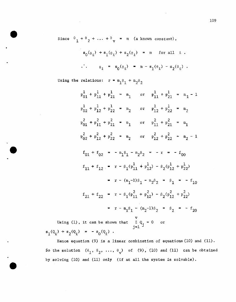
Since 81 + 8 2 + ... + 8 = m (a known constant) ,v

So (8 .Q,) +sl(8.Q,) + s2(8.Q,) = m for all .Q, .

8.Q, = SO(8.Q,) = m - sl(8.Q,) - s2(8.Q,) .

Using the relations: r = n1f\ + n2132

1 1 1 1 1POI + PH + P = n1 or Pn + P21 = n:l - 121

1 1 1 1 1P02 + P12 + P = n2 or P12 + P22 = n222

2 2 2 2 2POI +Pn + P21 = n1 or Pn + P21 n1

2 2 2 2 2P02 + P12 + P22 = n2 or P12 + P22 = n - 12

109

Using (1), it can be shown thatv1; Q. = 0

j=l Jor

Hence equation (9) is a linear combination of equations (10) and (11).

So the solution (81 , 82 , "', 8v

) of (9), (10) and (11) can be obtained

by solving (10) and (11) only (if at all the system is solvable).

...

no

the latter reduces to

__(12)

=

= (say) __(14)

=

__(15).

III

From (13) - (16) ,

hll + hZ1 = (£11 - f Ol) + (f1Z - f OZ )

= (f11 + f lZ) - (£01 + f 02)

= 13 - (-n l I3 1 - nZ13 2)1

= 13 1 + r .

Similarly it can be seen that

__(17)

__(18)

NOw coming back to (12) and writing gi(2) = si(Q£) - fOim, we have

Under the hypothesis we can show that the determinant of

H

is different from O.

-1Denoting H by

Before this

(

hll

h12

)

h2l

h22

evaluation, we note that

we can evaluate

112

=

for all £ = 1, 2, "', v .

Summing sl(8£) and

A A A

8£ == SO(8£) = m - sl(8£)

and using the relation

we have

By (19),

= m + (hll + h2l)folm + (h12 + h22)f02m

_ (hll + h

2l)sl(Q£) _ (h

12 + h22

)s2(Q£) (9)--

= sl(Q£)]

- s2(QQ,)] __(20)

(19) and (20) give the expressions for @£ and @£ - ~q Before evaluating

A A 1\ I .Var(8£) , and Var(8£ - 8q)' it can be ver1fied that HI ~ 0

hij can be found out. Further, (18) can be used to express h22

and

as

J 11

ell h1J (11~21 hdh2~j = ( ~r B:~:)I'-1 '

IHIhZ1 hzz hZ1 h ZZ h21

. (1 + r 1 B2+r Jr+Sz+piz (S z-f\)1\ (SZ-Sl)PIZ

(r + Sl)Z

(SZ - Sl) ]= r + Sz + P1Z

z Z 1= r + r[(Sl + Sz) + (Sz - Sl)(PIZ - P1Z)]

Z 1+ SlSZ + (Sz - Sl)[SlP1Z - SzP1Z ]

Since by hypothesis

- d1 ± hi - 4d Z

Z

IH I :f o.

__(21)

114

hZZ

Z . ( Z Z

hll P1l8 1 + PZZ + ZP1Z

+ 2)82 (l3a)

lHT ==Zr + d

1r + d

Z

-hZ1

1

h12 (Sl - SZ)P1Z (15a)= THT 2r + d1

r + dZ

-h1Z (S2

Z

h Z1 - Sl)P1Z (14a)= lHT = 2 + cl

1r + d

Zr

h ZZhll (Z 1 1 1

+ 2P12 + Pll)Sl + P22 BZ (l6a)= lHT Zr + d1

r + d2

where

and

THEOREM 6.3.2: Under the same conditions and with the same notation

as in Theorem 6.4, for ~ 1 q are given by:

and

115

1\ 1\ 2 13 1 2132pi2)var(e Q, - 8q) An [2n

l(r - 2 IPn

+2d'(I3B + 132B2

) e ] 02- 1 1

2 [r +Q, 13 (q 1 Q 2

+ 2A22131b ql

+ 132

bq2 - 1 buPn + b t2 Pll)

1 1r.~' (131

Bl + 132B2) ~]] 2+ nl(r - 2131Pll - 2132P12) + 0

where (hij) ) S are given on page 114 and

where

e d" = (b lb

2b

V)

ql ql ql

~'1 2 v

= (b .Q,1 , b U - , . . . bU

)

and All = (hll + h21) , A22 = (h12 + h 22 ) .

Proof: In order to find var(~Q,) and Var(~Q, - @q)' first we

evaluate (a) Var(Q,Q,)' (b) Cov(QQ,' Qq)' (c) Var[sl (Q,Q,)] ,

and

=

But

(a) Var(Q,Q,) =

Var(Q) = Var(N!.)

(b)

{ ,Q,-th diagonal element of Var(Q)} .

2 2 2= NN' 0 = (rI - 13 1B1 - 132B2)0 .'. Var(QQ,) = ro

= {,Q,-th row and q-th column element of Var(Q)f

,Q, ,Q, 2( - 13 1bq1 - 13 2bq2)0

(c)v i

= Var[ L: b 1Q. ]i=l i J.

v i v .= .L: b Ol Var(Q.) + 2 L: bJ.l b~l Cov(Q., Q )

J.=l N J. i#u=l Q, N J. U

116

whether ib Q,1 = 0 or 1.

2°

2 2 v u 2 v u-2810 L: P\lx,x -28 20 L: b'2x,x. 1 1. J. U . . 1 J. J. UJ.,u= J.,u=

where or the Q,-th row of Bl

.

•..2

- 28 °2

( Q,-th diagonal element of

( Q,-th diagonal element of

But

The Q,-th diagonal element = nlPil for all Q,.

117

1Hence the ~-th diagonal element = nlP1Z

.Var[sl(Q~)] n [r - 1 1 Z.. = Zf;\Pn ZSZP1Z]a1

nl(d) Cov[Q~, slCQ~)] = covC·L:1Q£..., Qg) = L: covCQC' Q~)

~= ~ ~

when ~i stands for any of the nl -first associates of ~-th treatment.

nl ~. ~. Z= - i:l (131bQ.~ + SZb Q.~) a

=

(e)

v

=

=

118

= _02

[(:31 E bUt1dteu + f3 2 E blid e' i:t, u t2, t-u

for the particular values of q and £.

by using part (d).

(g) =

=

if £ and q are the first associates and

if £ and q are

second associates.

(h)

119

A ANbw we can find out Var(8Q,) . By using the formula for eQ,

112+ 2 [nl (S1 - r + 2S l Pll + 2S2P12)]AllA220

__(17)*

by (c), (h), and (f).

Next by the formula forA Ae - eQ, q

But

Var[Ae - AS] = (hI1 + h2l)2 Var[s1(Qq) - sl(Qn)]Q, q N

12 22.2+ (h + h ) Var[s2(Qq) - s2(QQ,)]

11 21 12 22+ 2(h +h )(h +h )Cov[sl(Qq)-sl(QQ,),s2(Qq)-s2(QQ,)]

(18) *--

120

Hence

+ 2[Cov(Qt' sl(Qt) + Cov(Qq' sl(Qq» - Cov(Qq' sl (Qt» - Cov(Q~, sl(Qq»]

__(19)*

The expression in the last parenthesis is

by (d) and (g) •

__(20) *

•

Substituting (18)~ (19)*and (20)*in var[&9, - &q] , i.e. in (l7)~

we have

121

A lie]var[e9, - q

[2 ]

[1]

[5]

t)

122

BIBLIOGRAPHY

Adhikary, Basudeb (1965). "On the properties and the construction

of Balanced Block Designs with variable replications."

Calcutta Stat. Assoc. Bull., 14, 36-64.

Adhikary, Basudeb (1965). "A difference theorem for the con­

struction of Balanced Block Designs with variable replications."

Calcutta Stat. Assoc. Bull., 14, 167-70.

[3] Adhikary, Basudeb (1967). "A new type of Higher Associate

Cyclical Association Schemes." Calcutta Stat ".. Assoc. Bull.,

19, 40-44.

[4] Barra, J. R. (1965). "Carres Latins Et. Eu1eriens." Review of

the International Statistical Institute, 11, 16-23.

Blackwelder, William C. (1966). "Construction of Balanced

Incomplete Block Designs from Association Matrices."

Institute of Statistics Mimeo Series No. 481.

[6] Bose, R. C. (1963). "Combinatorial properties of partially

balanced designs and association schemes," Sankhya)£, 109-36.

[7] Bose, R. C. (1969). 'Combinatoria1 problems of Experimental

Designs. John Wiley and Sons, New York (to be pilblished)

[8] Bose, R. C. and B:ush~,K. A.> (19~2)~ . "Orth'bg.orial arrays of ('

st'rerigth 2 and 3. "Ann, Math • .sfiiUst. , . 23, 508"·24.

[9] Bose ,:R.:Ci:'"'an.d Gameron , ;S. M; (1965)., :~B1heBtidge-TOurnament

probleman.dcafibration designs for comparing pairs of

objects." Journal of Research of the National Bureau

of Standards, 69B, 323-32.

• [10 ]

123

Bose, R.C. and Cameron, J .M. (1967). "Calibration designs

based on solutions to the Tournament problem." Jour. of

Research 2.!... the National Bureau.£!. Standards, 7lB, 149-60.

[~l] Bose, R.C. and Shrikhande, S.S. and Bhattacharya, K.N. (1953).

"On the construction of group divisible incomplete block

designs." Ann. Math. ·Stat., ~, 167-95.

[12] Bose, R.C. and Clatworthy, W.H. and Shrikhande, S.S. (1954).

"Tables of partially balanced designs with two associate

classes." North Carolina~ Expt. Sta. Tech. Bull.,

,No. 107.

[13] Bose, R.C. and Connor, W.S. (1952). "Combinatorial properties

•of group divisible incomplete block designs."

Stat., 23, 367-83.

Ann. Math.----

•

[14] Bose, R.C. and Nair, K.R. (1939). "Partially Balanced Incomplete

Block designs." Sankhya, 4, 337-72.

[15] Bose, R.C. and Shimamoto, T. (1952). "Classification and analysis

of partially balanced incomplete block designs with two

associate classes." Jour. Amer. Stat. Assoc., 1:2, 151-84.

[16] Bose, R.C. and Shrikhande, S.S. (1960). "On the composition

of balanced incomplete block designs." ~ L Math., Q,

177-88.

[17] Chakravarti, LM. (1961). "On some methods of construction of

partially balanced arrays." Ann. Math. ~., E, 1181-85.

[18] Chakravarti, LM. (1963). "Orthogonal and partially balanced

arrays and their application in Design of Experiments."

Metrika, I, 231-43.

[22]

124

[19] Chakravarti, LM. (1965). "On the construction of difference

sets and their use in the search for othogonal Latin

Squares and error correcting codes. 1I Bulletin of the

International Statistical Institute, 10, 957-58.

[20] Clatworthy, W.H. (1956). "Contributions on Partially Balanced

Incomplete Block Designs with two associate classes."

National Bureau of Standards Applied Mathematics

Series, !!1..

[21] Clatworthy, W.H. (1956), "Contributions on Partially Balanced

Block Designs with two associate classes." National Bureau

of Standards Applied Mathematics Series, !!1..

CPilZl1Xan, W.G. and Cox, G.M. (1950). Experimental designs. '

Wiley Mathematical Statistics Series.

[23] Ehrenfeld, Sylvian (1955). "On the efficiencies of experimental

designs. 1I Ann. Math. Stat.,~, 247-55.

[24] Fisher, R.A. and Yates, F. (1953). Statistical tables for

biological, agricultural and medical research.

Oliver and Boyd.

[25] Hall, M., Jr. (1947). "Cyclic projective planes."

Duke Mathematical Jour., 14, 1079-90.

[26] Hall, M., Jr. (1956). IIA survey of difference sets. II

Proc. Amer. Math. Soc., 1, 975-86.

[27] Hall, M., Jr. (1968). IICombinatorial theory."

Blaisdell Publishing Company.

125

[28] Hotelling, H. (1944). "Some improvements in weighing and other

experimental techniques." Ann. Math. Stat., 15, 297-306.

[29] Kishen, K. (1945). "On the design of experiments. for weighing

and making other types of measurements." Ann. Math. Stat.,

16, 294-300.

[30] Mann, H.B. and Evans

Sankhya, 11, 357-64.

[31] Mann, H.B. (1965). "Addition theor.ems." Tracts in Mathematics,

18, Interscience Publishers.

[32] Mann, H.B. (1967). "Recent advances in difference sets."

Ann. Math. Monthly, ~, 229-35.

[33]

[34]

[36]

Mesner, Dale M. (1964). "Negative Latin Square designs,"

Institute of Statistics Mimeo Series No. 410.

Mood, A.M. (1946). "On Hote1ling I s weighing problem."

m -associate cyclical association

schemes. Roy. Memorial Volume.

[37] Peterson, W.W. (1961). "Error correcting codes."

The M.I.T. Press.

[38] Placket and Burman (1946). "The design of optimum multi-

factorial experiments." Biometrika, 33, 305-25.

[39] Raghavarao, D. (1959), "Some optimum weighing designs."

Ann. Math. Stat., 30, 295-303.

[40] Rankin, R.A. (1964). "Difference sets." Acta Arithmetic.. ,

2., 161-68.

(41) Rao, C.R. (1946). "On the hypercubes of strength d and a

system of confounding in factorial experiments."

Bull. Calcutta Math, Soc., ~, 67- 78.

[42] Rao, C.R. (1947). "Factorial arrangements derivable from

combinatorial arrangements of arrays." Jour. Roy.

Statistical Soc. (SuppI.), l, 128-39.

126

[43] Rao, C.R. (1965).

applications.

Linear Statistical inference and its

John Wiley and Sons, Inc.

[44]

[45]

Seiden, Esther (1954). "On the problem of construction of

orthogonal arrays." Ann. Math. Stat., 17,151-56.

Shrikhande, S.S. (1963). "Some recent developments on

mutually othogonal Latin Squares." Mathematics Student,

31, 167-77.

(46) Singer, J. (1938). "A theorem in finite projective geometry

and some applications to number theory."

Math. Soc., 43, 377-85.

Trans. Amer.

[47] Yamamoto, K. (1963). "Decomposition of difference sets."

Pacific Jour, Math. ,13, 337-52.

[48] Yates, F. (1935). "Complex experiments." Supp!. Jour.

Roy. Stat. Soc., 2, 181-247.

127

APPENDIX

TABLE 1

Parameters of Balanced Weighing designs from orthogonal arrays

v r p b A1A2_

6 10 2 15 2 4

6 10 2 15 2 4

4 3 2 3 1 2

12 22 6 22 10 12

8 7 4 7 3 4

8 7 4 7 3 4

TABLE 2

Parameters of Balanced Weighing designs from association matrices

v r p b A1A

2_

9 8 4 9 3 4

13 12 6 13 5 6

TABLE 3

Parameters of Balanced Weighing designs from orthogonal latin squares

89

~v_--=r:-.-_p~_-=b:....-_;.;.A1·_~A2_

3 12 2 3

f

,<l

128

TABLE 4

Parameters of Partially Balanced Weighing designs with cyclic association scheme

4.1. Use of Rule I

v r p b nl__n2__An----2.21__A12--A22-

29 14 7 29 14 14

61 30 15 61 30 30

S. No.

1

2

3

13 6 3 13 6 6 o

4

8

2

2

6

2

2

6

1

5

9

4.2 Use of Rule II

S.No. v r p b n1---!'!.2__A11--A21--A12--A22-

1 37 18 9 37 18 18 4 4 4 5

e 2 101 50 25 101 50 50 12 12 12 13

TABLE 5

Parameters of PBWD with triangular association scheme

S. :tb. v r p b n1---!'!.2__A11__A21--A12--A22-

1 10 6 2 15 6 3 1 2 0 0

2 21 20 3 70 10 10 4 6 0 0

3 10 6 2 15 6 3 1 2 0 0

4 10 6 3 10 6 3 2 2 0 2

5 15 4 3 10 8 6 1 0 0 2

6 10 36 2 90 6 3 6 8 0 8

7 15 24 2 90 8 6 3 0 0 8

e

c TABLE 6

Parameters of PBWD with L.S. association scheme

S.No. v r p b n1__n 2__AU __A21--A12--A22-

1 9 6 4 3 4 4 2 1 0 2

2 16 12 6 4 9 6 3 1 0 2

3 16 6 6 8 9 6 3 3 2 4

4 9 8 2 18 4 4 0 2 2 2

5 9 4 3 6 4 4 2 1 0 2

e 6 9 4 2 9 4 4 0 2 1 0

7 9 2Lj 2 ~4 4 4 6 4 0 8

129

TABLE 7

,~ Parameters of PBWD's with the singular GD association scheme

7(A) . Resolvable method

S. No. v r p b nl----!!.2--All--A21--A12--A22-

1 8 3 4 3 1 6 3 0 1 22 10 8 4 10 1 8 8 0 2 43 12 3 6 3 2 9 3 0 1 24 12 10 4 15 1 10 10 0 2 45 16 3 8 3 3 12 3 0 1 16 16 6 8 6 3 12 6 0 2 47 16 7 8 7 1 14 7 0 3 48 18 8 6 12 1 16 8 0 2 29 18 10 6 15 2 15 10 0 2 4

10 18 20 6 30 2 15 20 0 4 811 20 3 10 3 4 15 3 0 1 212 20 36 4 90 1 18 36 0 4 813 24 10 8 15 3 20 10 0 2 414 24 21 6 42 2 21 21 0 3 6

e 15 24 20 8 30 3 20 20 0 4 816 27 8 9 12 2 24 8 0 2 317 30 10 10 15 4. 25 15 0 2 418 30 28 6 70 L 28 28 0 4 619 30 36 6 90 2 27 36 0 4 820 30 20 : 10 30 4 25 2Gl 0 4 821 32 15 8 30 1 31 15 0 3 422 32 21 8 42 3. 28 2i 0 3 623 40 21 10 42 4 35 21 0 3 624 40 36 8 90 3 36 36 0 4 825 42 60 6 210 1 40 60 0 6 926 45 28 9 70 2 42 28 0 4 627 50 24 10 60 1 48 24 0 4 528 50 36 10 90 4 45 36 0 4 829 56 54 8 189 1 54 54 0 6 830 63 60 9 210 2 60 60 0 6 9

..

130

131

132

e 7 (C) . PBWD's of singular group divisible type using Theorem 5.4

S. No. v r p b n1__n2__All__A21--A12--A22- *..

1 12 '>4 (26)26 39 ' 1 24 12 0 1 22 26 60 10 78 1 24 60 0 20 25 (29)3 26 12 12 13 1 24 12 0 5 6 (30) ,4 26 8 6 18 2 24 8 0 1 2 (10)5 27 8 9 12 2 24 8 0 2 3 (11)6 27 8 12 9 2 24 8 0 3 4 (12)7 30 18 6 45 2 27 18 0 2 4 (13)8 30 18 9 30 2 27 18 0 2 3 (14)9 30 36 12 45 2 27 36 0 12 16 (15)

10 30 18 15 18 2 27 18 0 8 10 (16)11 22 10 10 11 1 20 10 0 4 5 (20)12 24 7 6 14 2 21 7 0 1 .2 (7)13 24 21 9 28 2 21 21 0 6 9 (8)14 24 7 12 7 2 21 7 0 3 4 (9)15 24 11 4 33 1 22 11 0 1 2 (21)16 24 11 6 22 1 22 11 0 2 .3 (22)17 24 22 8 33 1 22 22 0 6 8 (23)18 24 55 10 66 1 22 55 0 20 25 (24)19 24 11 12 11 1 22 11 0 5 6 (25)20 25 4 10 5 4 20 4 0 1 2 (2)

"" 21 26 12 4 39 1 24 12 0 4 6 (26)

e 22 26 6 6 26 1 24 6 0 2 .3 (27)23 18 10 9 10 2 15 10 0 4 6 (4)

.. 24 18 8 4 18 1 16 ·8 0 1 2 (10)25 20 3 10 3 4 15 3 0 1 2 (1)26 20 4 8 5 3 16 4 0 1 2 (2)27 20 18 4 45 1 18 18 0 2 4 (13)28 20 18 9 30 1 18 18 0 2 3 (14)29 20 36 8 45 1 18 36 0 12 16 (15)30 21 12 6 21 2 18 12 0 2 4 (5)31 21 6 9 . 7 2 18 6 0 2 3 (6)32 22 20 4 55 1 20 20 0 2 4 (17)33 22 30 6 55 1 20 30 0 6 9 (18)34 22 40 8 55 1 20 40 0 12 16 (19)35 18 8 6 12 1 16 8 0 2 3 (11)

36 18 8 8 9 1 16 8 0 3 4 (12)37 20 18 10 18 1 18 18 0 8 10 (16)38 8 3 4 3 1 6 3 0 1 2 (1)39 10 4 4 5 1 8 4 0 1 2 (2)40 12 3 6 3 2 9 3 0 1 2 (1)41 12 10 4 15 1 10 10 0 2 4 (3)

42 14 12 4 21 1 12 12 0 2 4 (5)43 14 6 6 7 1 12 6 0 2 3 (6)44 15 4 6 5 2 12 4 0 1 2 (2)45 16 3 8 3 3 12 3 0 1 2 (1)46 16 7 4 14 1 14 7 0 1 2 (7)e 47 16 21 6 28 1 14 21 0 6 .9 (8)48 16 7 8 7 1 14 7 0 3 4 (9)49 18 10 6 15 2 15 10 0 2 4 (3)

* Design number of the table on page 158 [10].

TABLE 8

Parameters of PBWD's with regular GD association scheme

133

S.No. v r p b nl__n2__An--,\21--Al2--A22-

1 6 8 2 12 1 4 0 4 2 3

2 10 8 2 20 1 8 0 0 1 2

3 16 6 2 24 3 12 2 0 0 1

v

e TABLE 9

•Parameters of PBWD's with semi-regular GD association scheme

1 12 10 3 20 1 10 o o 2 3

134

TABLE 9

Parameters of PBWD' s with semi-regular GD association scheme

•S. No. v r p b m n '\11--'\21--'\12--'\22-

• .f)

£ 1 6 2 2 3 3 2 2 0 0 12 6 4 2 6 3 2 0 4 1 13 6 4 2 6 3 2 4 0 0 24 6 6 2 9 3 2 6 0 0 35 6 8 2 12 3 2 0 8 2 26 6 10 2 15 3 2 10 0 0 57 8 3 2 6 4 2 3 0 0 18 8 3 3 4 4 2 0 3 1 19 8 6 2 8 4 2 6 0 0 2

10 8 6 3 8 4 2 0 6 2 211 8 9 2 18 4 2 9 0 0 312 9 8 3 12 3 3 8 0 0 413 9 10 3 15 3 3 10 0 0 514 10 4 2 10 5 2 4 0 0 115 10 4 4 5 5 2 4 0 1 216 10 6 3 10 5 2 4 2 1 217 10 8 2 20 5 2 0 8 1 118 10 8 2 20 5 2 8 0 0 2

'e 19 10 8 4 10 5 2 0 8 3 320 12 2 4 3 3 4 2 0 0 1

) 21 12 3 3 6 3 4 3 0 0 1." 22 12 4 4 6 3 4 4 0 0 2

23 12 5 2 15 3 4 5 0 0 124 12 5 3 10 3 4 0 5 1 125 12 5 5 6 3 4 0 5 2 226 12 6 3 12 3 4 6 0 0 227 12 6 4 9 3 4 6 0 0 328 12 8 4 12 3 4 8 0 0 429 12 9 3 18 3 4 9 0 0 330 12 10 2 30 3 4 10 0 0 231 12 10 2 30 3 4 0 10 1 132 12 10 3 20 3 4 0 10 2 233 12 10 4 15 3 ~. 10 0 0 5