
Contributions to Monte-Carlo Search · Contributions to Monte-Carlo Search David Lupien St-Pierre...
149
Contributions to Monte-Carlo Search David Lupien St-Pierre Montefiore Institute Li` ege University A thesis submitted for the degree of PhD in Engineering 2013 June
Transcript of Contributions to Monte-Carlo Search · Contributions to Monte-Carlo Search David Lupien St-Pierre...

Contributions to Monte-Carlo
Search
David Lupien St-Pierre
Montefiore Institute
Liege University
A thesis submitted for the degree of
PhD in Engineering
2013 June

ii

Acknowledgements
First and foremost, I would like to express my deepest gratitude and appre-
ciation to Prof. Quentin Louveaux, for offering me the opportunity to do
research at the University of Liege. Along these three years, he proved to
be a great collaborator on many scientific and human aspects. The present
work is mostly due to his support, patience, enthusiasm and creativity.
I would like to extend my deepest thanks to Prof. Damien Ernst for his up
to the point suggestions and advices regarding every research contribution
reported in this dissertation. His remarkable talent and research experience
have been very valuable at every stage of this research.
My deepest gratitude also goes to Dr. Francis Maes for being such an
inspiration in research, for his suggestions and for his enthusiasm.
A special acknowledgment to Prof. Olivier Teytaud, who was always very
supportive and helped me focus on the right ideas. I cannot count the
number of fruitful discussions that resulted from his deep understanding of
this work. More than this, I am glad to have met somebody with an equal
passion for games.
I also address my warmest thanks to all the SYSTMOD research unit, the
Department of Electrical Engineering and Computer Science, the GIGA
and the University of Liege, where I found a friendly and a stimulating
research environment. A special mention to Francois Schnitzler, Laurent
Poirrier, Raphael Fonteneau, Stephane Lens, Etienne Michel, Guy Lejeune,
Julien Becker, Gilles Louppe, Anne Collard, Samuel Hiard, Firas Safadi,
Laura Trotta and many other colleagues and friends from Monteore and
the GIGA that I forgot to mention here. I also would like to thank the
administrative staff of the University of Liege and, in particular, Charline
Ledent-De Baets and Diane Zander for their help.

Many thanks to the members of the jury for carefully reading this disserta-
tion and for their advice to improve its quality.
To you Zhen Wu, no words can express how grateful I feel for your uncon-
ditional support. Thank you for everything.
David Lupien St-Pierre
Liege,
June 2013

Abstract
This research is motivated by improving decision making under uncertainty
and in particular for games and symbolic regression. The present disser-
tation gathers research contributions in the field of Monte Carlo Search.
These contributions are focused around the selection, the simulation and
the recommendation policies. Moreover, we develop a methodology to au-
tomatically generate an MCS algorithm for a given problem.
For the selection policy, in most of the bandit literature, it is assumed that
there is no structure or similarities between arms. Thus each arm is in-
dependent from one another. In several instances however, arms can be
closely related. We show both theoretically and empirically, that a signifi-
cant improvement over the state-of-the-art selection policies is possible.
For the contribution on simulation policy, we focus on the symbolic regres-
sion problem and ponder on how to consistently generate different expres-
sions by changing the probability to draw each symbol. We formalize the
situation into an optimization problem and try different approaches. We
show a clear improvement in the sampling process for any length. We fur-
ther test the best approach by embedding it into a MCS algorithm and it
still shows an improvement.
For the contribution on recommendation policy, we study the most common
in combination with selection policies. A good recommendation policy is a
policy that works well with a given selection policy. We show that there is
a trend that seems to favor a robust recommendation policy over a riskier
one.
We also present a contribution where we automatically generate several
MCS algorithms from a list of core components upon which most MCS
algorithms are built upon and compare them to generic algorithms. The
results show that it often enables discovering new variants of MCS that
significantly outperform generic MCS algorithms.

iv

Contents
1 Introduction 1
1.1 Monte Carlo Search . . . . . . . . . . . . . . . . . . . . . . . . . . . . . 2
1.2 Multi-armed bandit problem . . . . . . . . . . . . . . . . . . . . . . . . 3
1.2.1 Computing rewards . . . . . . . . . . . . . . . . . . . . . . . . . 3
1.3 MCS algorithms . . . . . . . . . . . . . . . . . . . . . . . . . . . . . . . 5
1.4 Selection Policy . . . . . . . . . . . . . . . . . . . . . . . . . . . . . . . . 6
1.5 Simulation Policy . . . . . . . . . . . . . . . . . . . . . . . . . . . . . . . 7
1.6 Recommendation Policy . . . . . . . . . . . . . . . . . . . . . . . . . . . 8
1.7 Automatic MCS Algorithms Generation . . . . . . . . . . . . . . . . . . 9
2 Overview of Existing Selection Policies 11
2.1 Introduction . . . . . . . . . . . . . . . . . . . . . . . . . . . . . . . . . . 11
2.2 The game of Tron . . . . . . . . . . . . . . . . . . . . . . . . . . . . . . 13
2.2.1 Game description . . . . . . . . . . . . . . . . . . . . . . . . . . . 13
2.2.2 Game complexity . . . . . . . . . . . . . . . . . . . . . . . . . . . 14
2.2.3 Previous work . . . . . . . . . . . . . . . . . . . . . . . . . . . . . 15
2.3 Simultaneous Monte-Carlo Tree Search . . . . . . . . . . . . . . . . . . . 16
2.3.1 Monte-Carlo Tree Search . . . . . . . . . . . . . . . . . . . . . . 16
2.3.1.1 Selection . . . . . . . . . . . . . . . . . . . . . . . . . . 16
2.3.1.2 Expansion . . . . . . . . . . . . . . . . . . . . . . . . . 16
2.3.1.3 Simulation . . . . . . . . . . . . . . . . . . . . . . . . . 17
2.3.1.4 Backpropagation . . . . . . . . . . . . . . . . . . . . . . 17
2.3.2 Simultaneous moves . . . . . . . . . . . . . . . . . . . . . . . . . 17
2.4 Selection policies . . . . . . . . . . . . . . . . . . . . . . . . . . . . . . . 19
2.4.1 Deterministic selection policies . . . . . . . . . . . . . . . . . . . 19
v

CONTENTS
2.4.1.1 UCB1 . . . . . . . . . . . . . . . . . . . . . . . . . . . . 20
2.4.1.2 UCB1-Tuned . . . . . . . . . . . . . . . . . . . . . . . . 20
2.4.1.3 UCB-V . . . . . . . . . . . . . . . . . . . . . . . . . . . 21
2.4.1.4 UCB-Minimal . . . . . . . . . . . . . . . . . . . . . . . 21
2.4.1.5 OMC-Deterministic . . . . . . . . . . . . . . . . . . . . 22
2.4.1.6 MOSS . . . . . . . . . . . . . . . . . . . . . . . . . . . 22
2.4.2 Stochastic selection policies . . . . . . . . . . . . . . . . . . . . . 22
2.4.2.1 Random . . . . . . . . . . . . . . . . . . . . . . . . . . . 23
2.4.2.2 εn-greedy . . . . . . . . . . . . . . . . . . . . . . . . . . 23
2.4.2.3 Thompson Sampling . . . . . . . . . . . . . . . . . . . . 23
2.4.2.4 EXP3 . . . . . . . . . . . . . . . . . . . . . . . . . . . . 24
2.4.2.5 OMC-Stochastic . . . . . . . . . . . . . . . . . . . . . . 24
2.4.2.6 PBBM . . . . . . . . . . . . . . . . . . . . . . . . . . . 25
2.5 Experiments . . . . . . . . . . . . . . . . . . . . . . . . . . . . . . . . . . 25
2.5.1 Simulation heuristic . . . . . . . . . . . . . . . . . . . . . . . . . 25
2.5.2 Tuning parameter . . . . . . . . . . . . . . . . . . . . . . . . . . 26
2.5.3 Results . . . . . . . . . . . . . . . . . . . . . . . . . . . . . . . . 27
2.6 Conclusion . . . . . . . . . . . . . . . . . . . . . . . . . . . . . . . . . . 31
3 Selection Policy with Information Sharing for Adversarial Bandit 33
3.1 Introduction . . . . . . . . . . . . . . . . . . . . . . . . . . . . . . . . . . 33
3.2 Problem Statement . . . . . . . . . . . . . . . . . . . . . . . . . . . . . . 34
3.2.1 Nash Equilibrium . . . . . . . . . . . . . . . . . . . . . . . . . . . 35
3.2.2 Generic Bandit Algorithm . . . . . . . . . . . . . . . . . . . . . . 35
3.2.3 Problem Statement . . . . . . . . . . . . . . . . . . . . . . . . . . 36
3.3 Selection Policies and Updating rules . . . . . . . . . . . . . . . . . . . . 37
3.3.1 EXP3 . . . . . . . . . . . . . . . . . . . . . . . . . . . . . . . . . 37
3.3.2 TEXP3 . . . . . . . . . . . . . . . . . . . . . . . . . . . . . . . . 38
3.3.3 Structured EXP3 . . . . . . . . . . . . . . . . . . . . . . . . . . . 38
3.4 Theoretical Evaluation . . . . . . . . . . . . . . . . . . . . . . . . . . . . 39
3.5 Experiments . . . . . . . . . . . . . . . . . . . . . . . . . . . . . . . . . . 44
3.5.1 Artificial experiments . . . . . . . . . . . . . . . . . . . . . . . . 44
3.5.2 Urban Rivals . . . . . . . . . . . . . . . . . . . . . . . . . . . . . 46
vi

CONTENTS
3.6 Conclusion . . . . . . . . . . . . . . . . . . . . . . . . . . . . . . . . . . 48
4 Simulation Policy for Symbolic Regression 49
4.1 Introduction . . . . . . . . . . . . . . . . . . . . . . . . . . . . . . . . . . 49
4.2 Symbolic Regression . . . . . . . . . . . . . . . . . . . . . . . . . . . . . 50
4.3 Problem Formalization . . . . . . . . . . . . . . . . . . . . . . . . . . . . 51
4.3.1 Reverse polish notation . . . . . . . . . . . . . . . . . . . . . . . 52
4.3.2 Generative process to sample expressions . . . . . . . . . . . . . 54
4.3.3 Problem statement . . . . . . . . . . . . . . . . . . . . . . . . . . 55
4.4 Probability set learning . . . . . . . . . . . . . . . . . . . . . . . . . . . 56
4.4.1 Objective reformulation . . . . . . . . . . . . . . . . . . . . . . . 56
4.4.2 Instantiation and gradient computation . . . . . . . . . . . . . . 59
4.4.3 Proposed algorithm . . . . . . . . . . . . . . . . . . . . . . . . . 60
4.5 Combination of generative procedures . . . . . . . . . . . . . . . . . . . 62
4.6 Learning Algorithm for several Probability sets . . . . . . . . . . . . . . 66
4.6.1 Sampling strategy . . . . . . . . . . . . . . . . . . . . . . . . . . 67
4.6.2 Clustering . . . . . . . . . . . . . . . . . . . . . . . . . . . . . . . 67
4.6.2.1 Distances considered . . . . . . . . . . . . . . . . . . . . 68
4.6.2.2 Preprocessing . . . . . . . . . . . . . . . . . . . . . . . . 68
4.6.3 Meta Algorithm . . . . . . . . . . . . . . . . . . . . . . . . . . . 68
4.7 Experimental results . . . . . . . . . . . . . . . . . . . . . . . . . . . . . 68
4.7.1 Sampling Strategy: Medium-scale problems . . . . . . . . . . . . 71
4.7.2 Sampling Strategy: Towards large-scale problems . . . . . . . . . 73
4.7.3 Sampling Strategy: Application to Symbolic Regression . . . . . 74
4.7.4 Clustering: Parameter study . . . . . . . . . . . . . . . . . . . . 77
4.7.5 Clustering: Evaluation . . . . . . . . . . . . . . . . . . . . . . . . 79
4.8 Conclusion . . . . . . . . . . . . . . . . . . . . . . . . . . . . . . . . . . 80
5 Contribution on Recommendation Policy applied on Metagaming 83
5.1 Introduction . . . . . . . . . . . . . . . . . . . . . . . . . . . . . . . . . . 83
5.2 Recommendation Policy . . . . . . . . . . . . . . . . . . . . . . . . . . . 84
5.2.1 Formalization of the problem . . . . . . . . . . . . . . . . . . . . 84
5.2.2 Terminology, notations, formula . . . . . . . . . . . . . . . . . . . 87
5.3 Algorithms . . . . . . . . . . . . . . . . . . . . . . . . . . . . . . . . . . 88
vii

CONTENTS
5.3.1 Algorithms for exploration . . . . . . . . . . . . . . . . . . . . . . 88
5.3.2 Algorithms for final recommendation . . . . . . . . . . . . . . . . 89
5.4 Experimental results . . . . . . . . . . . . . . . . . . . . . . . . . . . . . 91
5.4.1 One-player case: killall Go . . . . . . . . . . . . . . . . . . . . . . 91
5.4.1.1 7x7 killall Go . . . . . . . . . . . . . . . . . . . . . . . . 91
5.4.1.2 13x13 killall Go . . . . . . . . . . . . . . . . . . . . . . 93
5.4.2 Two-player case: Sparse Adversarial Bandits for Urban Rivals . . 94
5.5 Conclusions . . . . . . . . . . . . . . . . . . . . . . . . . . . . . . . . . . 96
5.5.1 One-player case . . . . . . . . . . . . . . . . . . . . . . . . . . . . 97
5.5.2 Two-player case . . . . . . . . . . . . . . . . . . . . . . . . . . . 98
6 Algorithm discovery 101
6.1 Introduction . . . . . . . . . . . . . . . . . . . . . . . . . . . . . . . . . . 101
6.2 Problem statement . . . . . . . . . . . . . . . . . . . . . . . . . . . . . . 103
6.3 A grammar for Monte-Carlo search algorithms . . . . . . . . . . . . . . 104
6.3.1 Overall view . . . . . . . . . . . . . . . . . . . . . . . . . . . . . 104
6.3.2 Search components . . . . . . . . . . . . . . . . . . . . . . . . . . 105
6.3.3 Description of previously proposed algorithms . . . . . . . . . . . 109
6.4 Bandit-based algorithm discovery . . . . . . . . . . . . . . . . . . . . . . 111
6.4.1 Construction of the algorithm space . . . . . . . . . . . . . . . . 112
6.4.2 Bandit-based algorithm discovery . . . . . . . . . . . . . . . . . . 113
6.4.3 Discussion . . . . . . . . . . . . . . . . . . . . . . . . . . . . . . . 114
6.5 Experiments . . . . . . . . . . . . . . . . . . . . . . . . . . . . . . . . . . 115
6.5.1 Protocol . . . . . . . . . . . . . . . . . . . . . . . . . . . . . . . . 115
6.5.2 Sudoku . . . . . . . . . . . . . . . . . . . . . . . . . . . . . . . . 117
6.5.3 Real Valued Symbolic Regression . . . . . . . . . . . . . . . . . . 122
6.5.4 Morpion Solitaire . . . . . . . . . . . . . . . . . . . . . . . . . . . 126
6.5.5 Discussion . . . . . . . . . . . . . . . . . . . . . . . . . . . . . . . 127
6.6 Related Work . . . . . . . . . . . . . . . . . . . . . . . . . . . . . . . . . 129
6.7 Conclusion . . . . . . . . . . . . . . . . . . . . . . . . . . . . . . . . . . 130
7 Conclusion 133
References 135
viii

1
Introduction
I spent the past few years studying only one question: Given a list of choices, how to
select the best one(s)? It is a vast subject that is universal. Think about every time
one takes a decision and the process of taking it. Which beer to buy at the grocery,
which path to take when going to work or more difficult questions such as where to
invest your money (if you have any). Is there an optimal choice? Can we find it? Can
an algorithm do the same?
More specifically, the question that is of particular interest is how to make the
best possible sequence of decisions, a situation commonly encountered in production
planning, facility planning and in games. Games are especially well suited for studying
sequential decisions because you can test every crazy strategy without worrying about
the human cost on top of it. And let us face it, it is usually a lot of fun. Games are
used as a testbed for most of the contributions developed in the different chapters.
To find the best sequence of decisions might be relatively simple for a game like
Tic− Tac− Toe, even to some extent for a game like Chess, but what about modern
board games and video games where you have a gazillion possible sequences of choices
and limited time to decide.
In this thesis we discuss over the general subject of algorithms that take a sequence
of decisions under uncertainty. More specifically, we describe several contributions to
a specific class of algorithms called Monte-Carlo Search (MCS) Algorithms. In the
following we first introduce the notion of MCS algorithms in Section 1.1 and its general
framework in Section 1.2. Section 1.3 describes a classic MCS algorithm. Section 1.4,
1

1. INTRODUCTION
Section 1.5, Section 1.6 and Section 1.7 introduce the different contributions of the
thesis.
1.1 Monte Carlo Search
Monte-Carlo Search derives from Monte-Carlo simulation, which originated in the com-
puter of Los Alamos [1] and consists of a sequence of actions chosen at random. Monte-
Carlo simulations is at the heart of several state-of-the-art applications in diverse fields
such as finance, economics, biology, chemistry, optimization, mathematics and physics
[2, 3, 4, 5] to name a few.
There is no formal definition of Monte-Carlo Search (MCS) algorithms, yet it is
widely understood as a step-by-step procedure (algorithm) that relies on random simu-
lations (Monte Carlo) to extract information (search) from a space. MCS relies heavily
on the multi-armed bandit problem formalization that is introduced in Section 1.2.
What makes it so interesting in contrast to classic search algorithms is that it
does not rely on the knowledge of the problem beforehand. Prior to MCS, algorithms
designed to decide what is the best possible move to execute were mostly relying on an
objective function. An objective function is basically a function designed by an expert
in the field that decides which move is the best. Obviously the main problem with
this approach is that such a function seldom covers every situation encountered, and
the quality of the decision depends on the quality of the expert. Moreover, it is very
difficult to tackle new problems or problems where there is little information available.
MCS algorithms do not suffer from either of these drawbacks. All it requires is
a model of the problem at hand upon which they can execute (a lot of) simulations.
Here lies the strength of these algorithms. It is not in the ability to abstract like the
human brain, but in the raw computational power that computers excel. Computers
can do a lot of simulations very quickly and if needed simulations are suitable for
massive parallelization. More importantly, from an optimization point of view most
MCS algorithms can theoretically converge to the optimal decision given enough time.
Before the description of a well-known MCS algorithms, Section 1.2 first introduces the
underlying framework needed to define the algorithms.
2

1.2 Multi-armed bandit problem
1.2 Multi-armed bandit problem
The multi-armed bandit problem [6, 7, 8, 9] is a framework where one has to decide
which arm to play, how many times and/or in which order. For each arm there is
a reward associated, either deterministic or stochastic, and the objective is (usually)
to maximize the sum of rewards. Here arm is a generic term that can, for example,
represent a possible move in a given game.
Perhaps a simple example of a typical multi-armed bandit problem can help to
explain this framework. Imagine a gambler facing several slot machines. The gambler
objective is to select the slot machine (arm) that allows him to earn as much money
as possible. In other words, the gambler wants to maximize its cumulative reward or
minimize its regret, where the regret is the difference in gain between the best arm
and the one the gambler chose. In terms of games, the multi-armed bandit problem
generally translate into finding the move that leads toward the highest probability of
winning.
In order to do so, the gambler has to try different arms (explore) and then focus
(exploit) on the best one. This example clearly shows the dilemma between exploration
and exploitation. Imagine the gambler with a finite number of coins to spend. He wants
to find quickly the best arm and then select it over and over again. As the gambler
explores, he is more certain about which arm is the best, yet the coins spent exploring
are lost. On the opposite as the gambler exploits an arm, he can expect a specific
reward. He is however less certain about the fact that the he has chosen the best arm.
This dilemma is ever present in decision making and this framework embeds it fairly
well. Figure 1.1 shows a layout representation of a problem with 2 choices (think about
2 slot machines) and the reward is computed through a simulation represented here by
a wavy line. To find the best one, one can simply start from the root (the top node),
select a slot machine and get a reward through simulation. If such a process is repeated
enough times, we can compute the mean reward of each slot machine and finally make
an informed choice.
1.2.1 Computing rewards
From a pragmatic point of view, computing a reward can be a very difficult task. In the
previous example, the reward was rather straightforward to obtain as it was directly
3

1. INTRODUCTION
Figure 1.1: An example of 2 slot machines where the root node (at the top) is the starting
position. Each child represents a slot machine. The wavy line represents the simulation
process to evaluate the value of the reward.
given by the slot machine. However, anyone who played slot machines knows that we
do not win every turn. The best slot machine is the one that makes you win more often
(for a fixed reward). This ratio win/loss can be expressed in terms of probability and
is generally called a stochastic process. Stochasticity is one example that can make a
reward hard to compute. Because from the same initial setting 2 simulations can give 2
different rewards. One can overcome this problem by executing several simulations to
get an approximation of the true value of the reward, yet this increases the complexity
of an algorithm.
Another situation where a reward is difficult to compute can be explained through
an example. Imagine you are in the middle of a Chess game and try to evaluate the
value of a specific move. The reward here is given by the overall probability of winning
(there are others ways to evaluate a reward, this is simply for the sake of the example).
There are no stochastic process in the game of Chess, everything is deterministic, yet
what makes the reward hard to compute is the sheer number of possible sequences of
moves before the end of a game. Because there are so many possible combinations of
moves and the outcome vary greatly from one combination to another, it is difficult to
4

1.3 MCS algorithms
correctly evaluate.
In many games, these two characteristics are present which makes the computation
of a reward a difficult task. There is indeed a possible trade off between knowing the
exact reward and minimizing the complexity of an algorithm, but it is something to
bear in mind throughout this thesis.
1.3 MCS algorithms
In this section we present an iconic algorithm of the MCS class called Monte-Carlo Tree
Search (MCTS). MCTS is interesting because all contributions presented in this thesis
can be related to it.
Monte-Carlo Tree Search is a best-first search algorithm that relies on random
simulations to estimate the value of a move. It collects the results of these random
simulations in a game tree that is incrementally grown in an asymmetric way that favors
exploration of the most promising sequences of moves. This algorithm appeared in
scientific literature in 2006 in three different variants [10, 11, 12] and led to breakthrough
results in computer Go. Computer Go is a term that refers to algorithms playing the
game of Go.
In the context of games, the central data structure in MCTS is the game tree in
which nodes correspond to game states and edges correspond to possible moves. The
role of this tree is two-fold: it stores the outcomes of random simulations and it is used
to bias random simulations towards promising sequences of moves.
MCTS is divided in four main steps that are repeated until the time is up [13]:
Selection This step aims at selecting a node in the tree from which a new random
simulation will be performed.
Expansion If the selected node does not end the game, this step adds a new leaf
node (chosen randomly) to the selected one and selects this new node.
Simulation This step starts from the state associated to the selected leaf node, ex-
ecutes random moves in self-play until the end of the game and returns the result (in
games usually victory, defeat or draw). The use of an adequate simulation strategy can
improve the level of play [14].
5

1. INTRODUCTION
Backpropagation The backpropagation step consists in propagating the result of the
simulation backwards from the leaf node to the root.
Figure 1.2 shows the first three steps.
(a) Selection (b) Expansion (c) Simulation
Figure 1.2: Main steps of MCTS. Figure 1.2(a) shows the selection process. The node
in white represent the selected one. Figure 1.2(b) shows the expansion process. From
the selected node (in white) we simply add one node. Figure 1.2(c) shows the simulation
process (the wavy line) from the newly added node.
1.4 Selection Policy
The selection policy, also termed exploration policy, tree policy or even default policy
depending on the community, is the policy that tackles the exploration exploitation
dilemma within the tree. As its name suggests, it is related to the selection step (see
Figure 1.2). The way this step is performed is essential since it determines in which way
the tree is grown and how the computational budget is allocated to random simulations.
In MCTS, the selection step is performed by traversing the tree recursively from
the root node to a leaf node (a node where not all its children have been explored yet).
At each step of this traversal, we use a selection policy to select one of the child nodes
6
1.5 Simulation Policy
from the current one. It is a key component for the efficiency of an algorithm because
it regulates the trade off between exploration and exploitation.
There exist many different selection policies, yet they can be classified into 2 main
categories: Deterministic and Stochastic. The deterministic policies assign a value
for each possible arm and the selection is based upon a comparison of these values
(generally the arm with the highest value is selected). The stochastic policies assign a
probability to be selected for each arm. Chapter 2 formalizes the notion and studies
the most popular applied to the game of Tron. Our findings are cogent with the current
literature where the deterministic policies perform better than the stochastic ones.
In most of the bandit literature, it is assumed that there is no structure or simi-
larities between arms. Thus each arm are independent from one another. In games
however, arms can be closely related. The reasons for sharing information between
arms are threefold. First, each game possesses a specific set of rules. As such, there
is inherently an underlying structure that allows information sharing. Second, the
sheer number of possible actions can be too large to be efficiently explored. Third,
as mentioned in Section 1.2.1, to get a precise reward can be a difficult task. For in-
stance, it can be time consuming or/and involve highly stochastic processes. Under
such constraints, sharing information between arms seems a legitimate concept. Chap-
ter 3 presents a novel selection policy that makes use of the structure within a game.
The results, both theoretical and empirical, show a significant improvement over the
state-of-the-art selection policies.
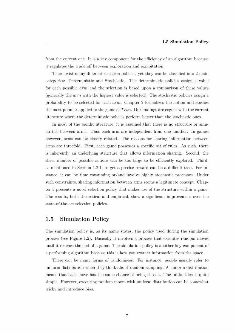
1.5 Simulation Policy
The simulation policy is, as its name states, the policy used during the simulation
process (see Figure 1.2). Basically it involves a process that executes random moves
until it reaches the end of a game. The simulation policy is another key component of
a performing algorithm because this is how you extract information from the space.
There can be many forms of randomness. For instance, people usually refer to
uniform distribution when they think about random sampling. A uniform distribution
means that each move has the same chance of being chosen. The initial idea is quite
simple. However, executing random moves with uniform distribution can be somewhat
tricky and introduce bias.
7

1. INTRODUCTION
How come? Instead of using games this time, we take as an example a toy problem
in Symbolic Regression (which can be viewed as a game if we get technical). In short,
Symbolic Regression means to generate expressions (formulas) from symbols. For in-
stance, with a set of symbols {a, b,+,−} and if we draw 3 consecutive symbols, only the
following valid expressions can be created: {a+a, b+b, a−b, b−a, a−a, b−b, a+b, b+a}.The probability to generate an expression is given by the multiplication of the
probability to draw each symbol. The problem becomes apparent when you take into
account the commutativity, distributivity and associativity property of an expression.
For instance, a − a and b − b are in fact the same expression 0. The same goes for
a + b and b + a. Thus, these 2 expressions are more likely to be randomly sampled
than other expressions. By using a uniform sampling over the symbols, in fact it leads
to a non-uniform sampling of the space. As the problem grows in size, there are a few
expressions that are repeatedly generated and others that are unlikely to be generated.
This simple example shows the importance of a relevant simulation policy.
In Chapter 4, we ponder on how to consistently generate different expressions by
changing the probability to draw each symbol. We formalize the situation into an
optimization problem and try different approaches. When the length of an expression
is relatively small (as in the simple example), it is easy to enumerate all the possible
combinations and validate our answer. However, we are interested into situations where
the length is too big to allow an enumeration (for instance a length of 25 or 30). We
show a clear improvement in the sampling process for any length. We further tested
the approach by embedding it into a MCS algorithm and it still shows an improvement.
1.6 Recommendation Policy
Sometimes the recommendation policy is confused with the selection policy. The dif-
ference is simple. The selection policy is used to gather information. It is designed to
tackle the trade off between exploration and exploitation. Such a trade off does not
exist when it is time to make a decision. Instinctively we usually just go for the best
move found so far.
So, a recommendation policy is the policy to use when we make the actual decision,
which has nothing to do with the strategy of how we gather the information. There is
no unique and universal recommendation policy. Simply put, it depends on what we
8

1.7 Automatic MCS Algorithms Generation
are looking for. For instance, do we want to make a robust (safe) decision, perhaps a
riskier one but with a potentially higher reward or a mix of both ?
In fact, the selection policy and the recommendation policy are mutually dependent.
A good recommendation policy is a policy that works well with a given selection policy.
There are several different strategies of recommendation and Chapter 5 studies the
most common in combination with selection policies. There is a trend that seems to
favor a robust recommendation policy over a riskier one.
1.7 Automatic MCS Algorithms Generation
The development of new MCS algorithms is mostly a manual search process. It usually
requires much human time and is error prone. Remember in Section 1.3 we defined
4 steps, or components, that represent the MCTS algorithm (Selection, Expansion,
Simulation and Backpropagation). In fact, if we take any MCS algorithm it is always
possible to break it down into smaller components. Chapter 6 presents a contribution
where the idea is to first list the core components upon which most MCS algorithms
are built upon.
Second, from this list of core components we automatically generate several MCS
algorithms and propose a methodology based on multi-armed bandits for identifying
the best MCS algorithm(s) for a given problem. The results show that it often enables
discovering new variants of MCS that significantly outperform generic MCS algorithms.
This contribution is significant because it presents an approach to provide a fully cus-
tomized MCS algorithm for a given problem.
9

1. INTRODUCTION
10

2
Overview of Existing Selection
Policies
2.1 Introduction
In this chapter we study the performance of different selection policies applied onto
an MCTS framework when the time allowed to gather information is rather small
(typically only a few hundred millisecond). This is an important question because
it requires efficient selection policies to gather the relevant information as rapidly as
possible.
Games provide a popular and challenging platform for research in Artificial Intelli-
gence (AI). Traditionally, the wide majority of work in this field focuses on turn-based
deterministic games such as Checkers [15], Chess [16] and Go [17]. These games are
characterized by the availability of a long thinking time (e.g. several minutes), making
it possible to develop large game trees before deciding which move to execute. Among
the techniques to develop such game trees, Monte-Carlo tree search (MCTS) is probably
the most important breakthrough of the last decade. This approach, which combines
the precision of tree-search with the generality of random simulations, has shown spec-
tacular successes in computer Go [12] and is now a method of choice for General Game
Playing (GGP) [18].
In recent years, the field has seen a growing interest for real-time games such as Tron
[19] and Miss Pac-Man [20], which typically involve short thinking times (e.g. 100 ms
per turn). Due to the real-time constraint, MCTS algorithms can only make a limited
11
2. OVERVIEW OF EXISTING SELECTION POLICIES
number of game simulations, which is typically several orders of magnitude less than
the number of simulations used in Go. In addition to the real-time constraint, real-
time video games are usually characterized by uncertainty, massive branching factors,
simultaneous moves and open-endedness. In this chapter, we focus on the game Tron,
for which simultaneous moves play a crucial role.
Applying MCTS to Tron was first proposed in [19], where the authors apply the
generic Upper Confidence bounds applied to Trees (UCT) algorithm to play this game.
In [21], several heuristics specifically designed for Tron are proposed to improve upon
the generic UCT algorithm. In both cases, the authors rely on the original UCT
algorithm that was designed for turn-based games. The simultaneous property of the
game is simply ignored. They use the algorithm as if players would take turn to play.
It is shown in [21] that this approximation generates artefacts, especially during the
last turns of a game. To reduce these artefacts, the authors propose a different way of
computing the set of valid moves, while still relying on the turn-based UCT algorithm.
In this chapter, we focus on variants of MCTS that explicitly take simultaneous
moves into account by only considering joint moves of both players. Adapting UCT
in this way has first been proposed by [22], with an illustration of the approach on
Rock-paper-scissors, a simple one-step simultaneous two-player game. Recently, the
authors of [23] proposed to use a stochastic selection policy specifically designed for
simultaneous two-player games: EXP3. They show that this stochastic selection policy
enables to outperform UCT on Urban Rivals, a partially observable internet card game.
The combination of simultaneous moves and short thinking time creates a unusual
setting for MCTS algorithms and has received little attention so far. On one side,
treating moves as simultaneous increases the branching factor and, on the other side,
the short thinking time limits the number of simulations that can be performed during
one turn. Algorithms such as UCT rely on a multi-armed bandit policy to select which
simulations to draw next. Traditional policies (e.g. UCB1 ) have been designed to
reach good asymptotic behavior [24]. In our case, since the ratio between the number
of simulations and the number of arms is relatively low, we may be far from reaching
this asymptotic regime, which makes it legitimate to wonder how other selection policies
would behave in this particular setting.
This chapter provides an extensive comparison of selection policies for MCTS ap-
plied to the simultaneous two-player real-time game Tron. We consider six deterministic
12

2.2 The game of Tron
selection policies (UCB1, UCB1-Tuned, UCB-V, UCB-Minimal, OMC-Deterministic
and MOSS ) and six stochastic selection policies (εn-greedy, EXP3, Thompson Sam-
pling, OMC-Stochastic, PBBM and Random). While some of these policies have al-
ready been proposed for Tron (UCB1, UCB1-Tuned), for MCTS (OMC-Deterministic,
OMC-Stochastic, PBBM ) or for simultaneous two-player games (εn-greedy, EXP3 ), we
also introduce four policies that, to the knowledge of the authors, have not been tried
yet in combination with MCTS: UCB-Minimal is a recently introduced policy that
was found through automatic discovery of good policies on multi-armed bandit prob-
lems [25], UCB-V is a policy that uses the estimated variance to obtain tighter upper
bounds [26], Thompson Sampling is a stochastic policy that has recently been shown
to behave very well on multi-armed bandit problems [27] and MOSS is a deterministic
policy that modifies the upper confidence bound of the UCB1 policy.
The outline of this chapter is as follows. Section 2.1 provides information on the
subject at hand. Section 2.2 first presents a brief description of the game of Tron.
Section 2.3 describes MCTS and details how we adapted MCTS to treat simultaneous
move. Section 2.4 describes the twelve selection policies that we considered in our
comparison. Section 2.5 shows obtained results and, finally, the conclusion and an
outlook of future search are covered in Section 2.6.
2.2 The game of Tron
This section introduces the game Tron, discusses its complexity and reviews previous
AI work for this game.
2.2.1 Game description
The Steven Lisberger’s film Tron was released in 1982 and features a Snake-like game.
This game, illustrated in Figure 2.1, occurs in a virtual world where two motorcycles
move at constant speed making only right angle turns. The two motorcycles leave solid
wall trails behind them that progressively fill the arena, until one player or both crashes
into one of them.
Tron is played on a N ×M grid of cells in which each cell can either be empty or
occupied. Commonly, this grid is a square, i.e. N = M . At each time step, both players
move simultaneously and can only (a) continue straight ahead, (b) turn right or (c)
13

2. OVERVIEW OF EXISTING SELECTION POLICIES
Figure 2.1: Illustration of the game of Tron on a 20× 20 board.
turn left. A player cannot stop moving, each move is typically very fast (e.g. 100 ms per
step) and the game is usually short. The goal is to survive his opponent until he crashes
into a wall. The game can finish in a draw if the two players move at the same position
or if they both crash at the same time. The main strategy consists in attempting to
reduce the movement space of the opponent. For example, in the situation depicted in
Figure 2.1, player 1 has a bigger share of the board and will probably win.
Tron is a finite-length game: the number of steps is upper bounded by N×M2 . In
practice, the number of moves in a game is often much lower since one of the player
can usually quickly confine his opponent within a small area, leading to a quick end of
the game.
Tron became a popular game implemented in a lot of variants. A well-known
variant is the game “Achtung, die kurve!”, that includes bonuses (lower and faster
speed, passing through the wall, etc.) and curve movements.
2.2.2 Game complexity
Several ways of measuring game complexity have been proposed and studied in game
theory, among which game tree size, game-tree complexity and computational com-
plexity [28]. We discuss here the game-tree complexity of Tron. Since moves occur
simultaneously, each possible pair of moves must be considered when developing a
14

2.2 The game of Tron
node in the game tree. Given that agents have three possible moves (go straight, turn
right and turn left), there exists 32 pairs of moves for each state, hence the branching
factor of the game tree is 9.
We can estimate the mean game-tree complexity by raising the branching factor to
the power of the mean length of games. It is shown in [29], that the following formula
is a reasonable approximation of the average length of the game:
a =N2
1 + log2N
for a symmetric game N = M . In this chapter, we consider 20 × 20 boards and have
a ' 75. Using this formula, we obtain that the average tree-complexity for Tron on a
20× 20 board is O(1071). If we compare 20× 20 and 32× 32 Tron to some well-known
games, we obtain the following ranking:
Draughts(1054) < Tron20×20(1071) < Chess(10123)
< Tron32×32(10162) < Go19×19(10360)
Tron has been studied in graph and game complexity theory and has been proven
to be PSPACE -complete, i.e. to be a decision problem which can be solved by a Turing
machine using a polynomial amount of space and every other problem that can be
solved in polynomial space can be transformed to it in polynomial time [30, 31, 32].
2.2.3 Previous work
Different techniques have been investigated to build agents for Tron. The authors of
[33, 34] introduced a framework based on evolutionary algorithms and interaction with
human players. At the core of their approach is an Internet server that enables to per-
form agent vs. human games to construct the fitness function used in the evolutionary
algorithm. In the same spirit, [35] proposed to train a neural-network based agent by
using human data. Turn-based MCTS has been introduced in the context of Tron in
[19] and [29] and further developed with domain-specific heuristics in [21].
Tron was used in the 2010 Google AI Challenge, organised by the University of
Waterloo Computer Science Club. The aim of this challenge was to develop the best
agent to play the game using any techniques in a wide range of possible programming
15

2. OVERVIEW OF EXISTING SELECTION POLICIES
languages. The winner of this challenge was Andy Sloane who implemented an Alpha-
Beta algorithm with an evaluation function based on the tree of chambers heuristic1.
2.3 Simultaneous Monte-Carlo Tree Search
This section introduces the variant of MCTS that we use to treat simultaneous moves.
We start with a brief description of the classical MCTS algorithm.
2.3.1 Monte-Carlo Tree Search
Monte-Carlo Tree Search is a best-first search algorithm that relies on random simula-
tions to estimate position values. MCTS collects the results of these random simulations
in a game tree that is incrementally grown in an asymmetric way that favors explo-
ration of the most promising sequences of moves. This algorithm appeared in scientific
literature in 2006 in three different variants [11, 36, 37] and led to breakthrough results
in computer Go. Thanks to the generality of random simulations, MCTS can be applied
to a wide range of problems without requiring any prior knowledge or domain-specific
heuristics. Hence, it became a method of choice in General Game Playing.
The central data structure in MCTS is the game tree in which nodes correspond to
game states and edges correspond to possible moves. The role of this tree is two-fold:
it stores the outcomes of random simulations and it is used to bias random simulations
towards promising sequences of moves.
MCTS is divided in four main steps that are repeated until the time is up [13]:
2.3.1.1 Selection
This step aims at selecting a node in the tree from which a new random simulation will
be performed.
2.3.1.2 Expansion
If the selected node does not end the game, this steps adds a new leaf node to the
selected one and selects this new node.
1http://a1k0n.net/2010/03/04/google-ai-postmortem.html
16
2.3 Simultaneous Monte-Carlo Tree Search
2.3.1.3 Simulation
This step starts from the state associated to the selected leaf node, executes random
moves in self-play until the end of the game and returns the following reward: 1 for a
victory, 0 for a defeat or 0.5 for a draw. The use of an adequate simulation strategy
can improve the level of play [14].
2.3.1.4 Backpropagation
The backpropagation step consists in propagating the result of the simulation backwards
from the leaf node to the root.
The main focus of this chapter is on the selection step. The way this step is
performed is essential since it determines in which way the tree is grown and how
the computational budget is allocated to random simulations. It has to deal with
the exploration/exploitation dilemma: exploration consists in trying new sequences of
moves to increase knowledge and exploitation consists in using current knowledge to
bias computational efforts towards promising sequences of moves.
When the computational budget is exhausted, one of the moves is selected based
on the information collected from simulations and contained in the game tree. In this
chapter, we use the strategy called robust child, which consists in choosing the move
that has been most simulated.
2.3.2 Simultaneous moves
In order to properly account for simultaneous moves, we follow a strategy similar to the
one proposed in [22, 23]: instead of selecting a move for the agent, updating the game
state and then selecting an action for its opponent, we select both actions simultane-
ously and independently and then update the state of the game. Since we treat both
moves simultaneously, edges in the game tree are associated to pairs of moves (α, β)
where α denotes the move selected by the agent and β denotes the move selected by
its opponent.
Let N be the set of nodes in the game tree and n0 ∈ N be the root node of the
game tree. Our selection step is detailed in Algorithm 1. It works by traversing the
tree recursively from the root node n0 to a leaf node n ∈ N. We denote by M the set of
possible moves. Each step of this traversal involves selecting moves α ∈M and β ∈M
17

2. OVERVIEW OF EXISTING SELECTION POLICIES
Algorithm 1 Simultaneous two-players selection procedure. The main loop consists
of choosing independently a move for both α and β and select the corresponding child
node.Require: The root node n0 ∈ N
Require: The selection policy π(·) ∈M
n← n0
while n is not a leaf do
α← π(P agent(n))
β ← π(P opponent(n))
n← child(n, (α, β))
end while
return n
and moving into the corresponding child node, denoted child(n, (α, β)). The selection
of a move is done in two steps: first, a set of statistics P player(n) is extracted from the
game tree to describe the selection problem and then, a selection policy π is invoked
to choose the move given this information. The rest of this section details these two
steps.
For each node n ∈ N, we store the following quantities:
� t(n) is the number of simulations involving node n, which is known as the visit
count of node n.
� r(n) is the empirical mean of the rewards the agent obtained from these sim-
ulations. Note that because it is a one-sum game, the average reward for the
opponent is 1− r(n).
� σ(n) is the empirical standard deviation of the rewards (which is the same for
both players).
Let Lagent(n) ⊂M (resp. Lopponent(n) ⊂M) be the set of legal moves for the agent
(resp. the opponent) in the game state represented by node n. In the case of Tron,
legal moves are those that do not lead to an immediate crash: e.g. turning into an
already existing wall is not a legal move1.
Let player ∈ {agent, opponent}. The function P player(·) computes a vector of statis-
tics S = (m1, r1, σ1, t1, . . . ,mK , rK , σK , tK) describing the selection problem from the
1If the set of legal moves is empty for one of the players, this player loses the game.
18

2.4 Selection policies
point of view of player. In this vector, {m1, . . . ,mK} = Lplayer(n) is the set of valid
moves for the player and ∀k ∈ [1,K], rk, σk and tk are statistics relative to the move
mk. We here describe the statistics computation in the case of P agent(·). Let C(n, α)
be the set of child nodes whose first action is α, i.e. C(n, α) = {child(n, α, β)|β ∈Lopponent(n)}. For each legal move mk ∈ Lagent(n), we compute:
tk =∑
n′∈C(n,mk)
t(n′),
rk =
∑n′∈C(n,mk) t(n
′)r(n′)
tk,
σk =
∑n′∈C(n,mk) t(n
′)σ(n′)
tk.
P opponent(·) is simply obtained by taking the symmetric definition of C: i.e. C(n, β) =
{child(n, α, β)|α ∈ Lplayer(n)}.The selection policy π(·) ∈M is an algorithm that selects a movemk ∈ {m1, . . . ,mK}
given the vector of statistics S = (m1, r1, σ1, t1, . . . ,mK , rK , σK , tK). Selection policies
are the topic of the next section.
2.4 Selection policies
This section describes the twelve selection policies that we use in our comparison.
We first describe deterministic selection policies and then move on stochastic selection
policies.
2.4.1 Deterministic selection policies
We consider deterministic selection policies that belong to the class of index-based
multi-armed bandit policies. These policies work by assigning an index to each can-
didate move and by selecting the move with maximal index: πdeterministic(S) = mk∗
with
k∗ = argmaxk∈[1,K]
index(tk, rk, σk, t)
where t =∑K
k=1 tk and index is called the index function. Index functions typically
combine an exploration term to favor moves that we already know perform well with an
19

2. OVERVIEW OF EXISTING SELECTION POLICIES
exploitation term that aims at selecting less-played moves that may potentially reveal
interesting. Several index-policies have been proposed and they vary in the way they
define these two terms.
2.4.1.1 UCB1
The index function of UCB1 [24] is:
index(tk, rk, σk, t) = rk +
√C
ln t
tk,
where C > 0 is a parameter that enables to control the exploration/exploitation trade-
off. Although the theory suggest a default value of C = 2, this parameter is usually
experimentally tuned to increase performance.
UCB1 has appeared the first time in the literature in 2002 and is probably the best
known index-based policy for multi-armed bandit problem [24]. It has been popularized
in the context of MCTS with the Upper confidence bounds applied to Trees (UCT)
algorithm [36], which is the instance of MCTS using UCB1 as selection policy.
2.4.1.2 UCB1-Tuned
In their seminal paper, the authors of [24] introduced another index-based policy called
UCB1-Tuned, which has the following index function:
index(tk, rk, σk, t) = rk +
√min{1
4 , V (tk, σk, t)} ln t
tk,
where
V (tk, σk, t) = σ2k +
√2 ln t
tk.
UCB1-Tuned relies on the idea to take empirical standard deviations of the rewards
into account to obtain a refined upper bound on rewards expectation. It is analog
to UCB1 where the parameter C has been replaced by a smart upper bound on the
variance of the rewards, which is either 14 (an upper bound of the variance of Bernouilli
random variable) or V (tk, σk, t) (an upper confidence bound computed from samples
observed so far).
Using UCB1-Tuned in the context of MCTS for Tron has already been proposed
by [19]. This policy was shown to behave better than UCB1 on multi-armed bandit
problems with Bernouilli reward distributions, a setting close to ours.
20

2.4 Selection policies
2.4.1.3 UCB-V
The index-based policy UCB-V [26] uses the following index formula:
index(tk, rk, σk, t) = rk +
√2σ2kζ ln t
tk+ c
3ζ ln t
tk.
UCB-V has two parameters ζ > 0 and c > 0. We refer the reader to [26] for
detailed explanations of these parameters.
UCB-V is a less tried multi-armed bandit policy in the context of MCTS. As UCB1-
Tuned, this policy relies on the variance of observed rewards to compute tight upper
bound on rewards expectation.
2.4.1.4 UCB-Minimal
Starting from the observation that many different similar index formulas have been
proposed in the multi-armed bandit literature, it was recently proposed in [25, 38] to
explore the space of possible index formulas in a systematic way to discover new high-
performance bandit policies. The proposed approach first defines a grammar made of
basic elements (mathematical operators, constants and variables such as rk and tk) and
generates a large set of candidate formulas from this grammar. The systematic search
for good candidate formulas is then carried out by a built-on-purpose optimization
algorithm used to navigate inside this large set of candidate formulas towards those
that give high performance on generic multi-armed bandit problems. As a result of this
automatic discovery approach, it was found that the following simple policy behaved
very well on several different generic multi-armed bandit problems:
index(tk, rk, σk, t) = rk +C
tk,
where C > 0 is a parameter to control the exploration/exploitation tradeoff. This
policy corresponds to the simplest form of UCB-style policies. In this chapter, we
consider a slightly more general formula that we call UCB-Minimal :
index(tk, rk, σk, t) = rk +C1
tC2k
,
where the new parameter C2 enables to fine-tune the decrease rate of the exploration
term.
21

2. OVERVIEW OF EXISTING SELECTION POLICIES
2.4.1.5 OMC-Deterministic
The Objective Monte-Carlo (OMC ) selection policy exists in two variants: stochastic
(OMC-Stochastic) [11] and deterministic (OMC-Deterministic) [39]. The index-based
policy for OMC-Deterministic is computed in two steps. First, a value Uk is computed
for each move k:
Uk =2√π
∫ ∞α
e−u2du,
where α is given by:
α =v0 − (rktk)√
2σk,
and where
v0 = max(riti) ∀i ∈ [1,K].
After that, the following index formula is used:
index(tk, rk, σk, t) =tUk
tkK∑i=1
Ui
.
2.4.1.6 MOSS
Minimax Optimal Strategy in the Stochastic Case (MOSS ) is an index-based policy
proposed in [40] where the following index formula is introduced:
index(tk, rk, σk, t) = rk +
√max
(log(tkKt
), 0)
t.
This policy is inspired from the UCB1 policy. The index of a move is the mean
of rewards obtained from simulations if the move has been selected more than tkK .
Otherwise, the index value is an upper confidence bound on the mean reward. This
bound holds with a high probability according the Hoeffding’s inequality. Similarly to
UCB1-Tuned, this selection policy has no parameters to tune thus facilitating its use.
2.4.2 Stochastic selection policies
In the case of simultaneous two-player games, the opponent’s moves are not immedi-
ately observable, and following the analysis of [23], it may be beneficial to also consider
22

2.4 Selection policies
stochastic selection policies. Stochastic selection policies π are defined through a con-
dition distribution pπ(k|S) of moves given the vector of statistics S:
πstochastic(S) = mk, k ∼ pπ(·|S).
We consider six stochastic policies:
2.4.2.1 Random
This baseline policy simply selects moves with uniform probabilities:
pπ(k|S) =1
K, ∀k ∈ [1,K].
2.4.2.2 εn-greedy
The second baseline is εn-greedy [41]. This policy consists in selecting a random move
with low probability εt or the empirical best move according to rk:
pπ(k|S) =
{1− εt if k = argmaxk∈[1,K] rk
εt/K otherwise.
The amount of exploration εt is chosen to decrease with time. We adopt the scheme
proposed in [24]:
εt =c K
d2 t,
where c > 0 and d > 0 are tunable parameters.
2.4.2.3 Thompson Sampling
Thompson Sampling adopts a Bayesian perspective by incrementally updating a belief
state for the unknown reward expectations and by randomly selecting actions according
to their probability of being optimal according to this belief state.
We consider here the variant of Thompson Sampling proposed in [27] in which the
reward expectations are modeled using a beta distribution. The sampling procedure
works as follows: it first draw a stochastic score
s(k) ∼ beta(C1 + rkt, C2 + (1− rk)tk
)for each candidate move k ∈ [1,K] and then selects the move maximizing this score:
pπ(k|S) =
{1 if k = argmaxk∈[1,K] s(k)
0 otherwise.
23

2. OVERVIEW OF EXISTING SELECTION POLICIES
C1 > 0 and C2 > 0 are two tunable parameters that reflect prior knowledge on reward
expectations.
Thompson Sampling has recently been shown to perform very well on Bernouilli
multi-armed bandit problems, in both context-free and contextual bandit settings [27].
The reason why Thompson Sampling is not very popular yet may be due to his lack of
theoretical analysis. At this point, only the convergence has been proved [42].
2.4.2.4 EXP3
This stochastic policy is commonly used in simultaneous two-player games [23, 43, 44]
and is proved to converge towards the Nash equilibrium asymptotically. EXP3 works
slightly differently from our other policies since it requires storing two additional vectors
in each node n ∈ N denoted wagent(n) and wopponent(n). These vectors contain one
entry per possible move m ∈ Lplayer, are initialized to wplayerk (·) = 0, ∀k ∈ [1,K] and
are updated each time a reward r is observed, according to the following formulas:
wagentk (n)← wagentk (n) +r
pπ(k|P agent(n)),
wopponentk (n)← wopponentk (n) +1− r
pπ(k|P opponent(n)).
At any given time step, the probabilities to select a move are defined as:
pπ(k|S) = (1− γ)eηw
playerk (n)∑
k′∈[1,K]
eηwplayer
k′+γ
K,
where η > 0 and γ ∈]0; 1] are two parameters to tune.
2.4.2.5 OMC-Stochastic
The OMC-Stochastic selection policy [11] uses the same Uk quantities than OMC-
Deterministic. The stochastic version of this policy is defined as following:
pπ(k|S) =UkK∑i=1
Ui
∀k ∈ [1,K].
The design of this policy is based on the Central Limit Theorem and EXP3.
24

2.5 Experiments
2.4.2.6 PBBM
Probability to be Better than Best Move (PBBM ) is a selection policy [12] with a
probability proportional to
pπ(k|S) = e−2.4α ∀k ∈ [1,K].
The α is computed as:
α =v0 − (rktk)√2(σ2
0 + σ2k),
where
v0 = max(riti) ∀i ∈ [1,K],
and where σ20 is the variance of the reward for the move selected to compute v0.
This selection policy was successfully used in Crazy Stone, a computer Go program
[12]. The concept is to select the move according to its probability of being better than
the current best move.
2.5 Experiments
In this section we compare the selection policies π(·) presented in Section 2.4 on the
game of Tron introduced previously in this chapter. We start this section by first
describing the strategy used for simulating the rest of the game when going beyond
a terminal leaf of the tree (Section 2.5.1). Afterwards, we will detail the procedure
we adopted for tuning the parameters of the selection policies (Section 2.5.2). And,
finally, we will present the metric used for comparing the different policies and discuss
the results that have been obtained (Section 2.5.3).
2.5.1 Simulation heuristic
It has already been recognized for a long time that using pure random strategies for
simulating the game beyond a terminal leaf node of the tree built by MCTS techniques
is a suboptimal choice. Indeed, such a random strategy may lead to a game outcome
that poorly reflects the quality of the selection procedure defined by the tree. This
in turn requires to build large trees in order to compute high-performing moves. To
define our simulation heuristic we have therefore decided to use prior knowledge on
25

2. OVERVIEW OF EXISTING SELECTION POLICIES
the problem. Here, we use a simple heuristic developed in [29] for the game on Tron
that, even if still far from an optimal strategy, lead the two players to adopt a more
rationale behaviour. This heuristic is based on a distribution probability Pmove(·) over
the moves that associates a probability of 0.68 to the “go straight ahead” move and
a probability of 0.16 to each of the two other moves (turn left or right). Afterwards,
moves are sequentially drawn from Pmove(·) until a move that is legal and that does not
lead to self-entrapment at the next time step is found. This move is the one selected
by our simulation strategy.
To prove the efficiency of this heuristic, we performed a short experiment. We
confronted two identical UCT opponents on 10 000 rounds: one using the heuristic and
the other making purely random simulations. The result of this experiment is that the
agent with the heuristic has a winning percentage of 93.42± 0.5% in a 95% confidence
interval.
Note that the performance of the selection policy depends on the simulation strategy
used. Therefore, we cannot exclude that if a selection policy is found to behave better
than another one for a given simulation strategy, it may actually behave worse for
another one.
2.5.2 Tuning parameter
The selection policies have one or several parameters to tune. Our protocol to tune
these parameters is rather simple and is the same for every selection policy.
First, we choose for the selection policy to tune reference parameters that are used
to define our reference opponent. These reference parameters are chosen based on
default values suggested in the literature. Afterwards, we discretize the parameter
space of the selection policy and test for every element of this set the performance of
the corresponding agent against the reference opponent. The element of the discretized
space that leads to the highest performance is then used to define the constants.
To test the performance of an agent against our reference opponent, we used the
following experimental protocol. First, we set the game map to 20 × 20 and the time
between two recommendations to 100 ms on a 2.5Ghz processor. Afterwards we perform
a sequence of rounds until we have 10,000 rounds that do not end by a draw. Finally,
we set the performance of the agent to its percentage of winnings.
26

2.5 Experiments
Table 2.1: Reference and tuned parameters for selection policies
Agent Reference constant Tuned
UCB1 C = 2 C = 3.52
UCB1-Tuned – –
UCB-V c = 1.0, ζ = 1.0 c = 1.68, ζ = 0.54
UCB-Minimal C1 = 2.5, C2 = 1.0 C1 = 8.40, C2 = 1.80
OMC-Deterministic – –
MOSS – –
Random – –
εn-greedy c = 1.0, d = 1.0 c = 0.8, d = 0.12
Thompson Sampling C1 = 1.0, C2 = 1.0 C1 = 9.6, C2 = 1.32
EXP3 γ = 0.5 γ = 0.36
OMC-Stochastic – –
PBBM – –
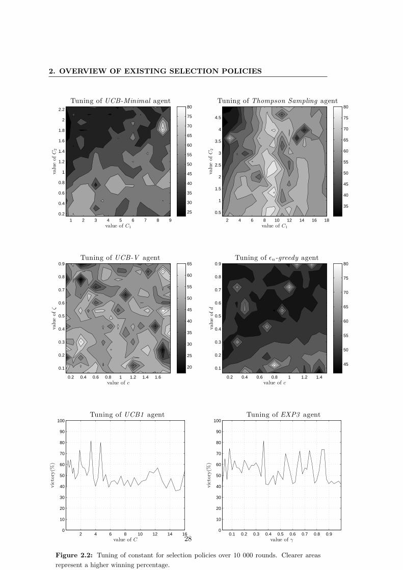
Figure 2.2 reports the performances obtained by the selection policies on rather large
discretized parameter spaces. The best parameters found for every selection policy as
well as the reference parameters are given in Table 2.1. Some side simulations have
shown that even by using a finer disretization of the parameter space, significantly
better performing agents cannot not be found.
It should be stressed that the tuned parameters reported in this table point towards
higher exploration rates than those usually suggested for other games, such as for
example the game of Go. This is probably due to the low branching factor of the game
of Tron combined with the fact that we use the robust child recommendation policy.
Even though after 10 000 the standard error of the mean (SEM) is rather low, the
behavior of some curves seems to indicate potential noise. We leave as future research
the study of the impact of the simluation policy on the noise.
2.5.3 Results
27
2. OVERVIEW OF EXISTING SELECTION POLICIES
Tuning of UCB-Minimal agent
value of C1
valueofC
2
1 2 3 4 5 6 7 8 90.2
0.4
0.6
0.8
1
1.2
1.4
1.6
1.8
2
2.2
Tuning of Thompson Sampling agent
value of C1
valueofC
2
2 4 6 8 10 12 14 16 18
0.5
1
1.5
2
2.5
3
3.5
4
4.5
Tuning of UCB-V agent
value of c
valueofζ
0.2 0.4 0.6 0.8 1 1.2 1.4 1.6
0.1
0.2
0.3
0.4
0.5
0.6
0.7
0.8
0.9Tuning of ǫn-greedy agent
value of c
valueofd
0.2 0.4 0.6 0.8 1 1.2 1.4
0.1
0.2
0.3
0.4
0.5
0.6
0.7
0.8
0.9
2 4 6 8 10 12 14 160
10
20
30
40
50
60
70
80
90
100Tuning of UCB1 agent
value of C
victory(%
)
0.1 0.2 0.3 0.4 0.5 0.6 0.7 0.8 0.90
10
20
30
40
50
60
70
80
90
100Tuning of EXP3 agent
value of γ
victory(%
)25
30
35
40
45
50
55
60
65
70
75
80
35
40
45
50
55
60
65
70
75
80
20
25
30
35
40
45
50
55
60
65
45
50
55
60
65
70
75
80
Figure 2.2: Tuning of constant for selection policies over 10 000 rounds. Clearer areas
represent a higher winning percentage.
28

2.5
Exp
erim
ents
Table 2.2: Percentage of victory on 10 000 rounds between selection policies
hhhhhhhhhhhhhhhhhhhhSelection policies
Selection policiesUCB1-Tuned UCB1 MOSS UCB-Minimal EXP3 Thompson Sampling εn-greedy OMC-Deterministic UCB-V OMC-Stochastic PBBM Random Average
UCB1-Tuned – 60.11 ± 0.98% 59.14 ± 0.98% 53.14 ± 1.00% 91.07 ± 0.57% 80.79 ± 0.80% 86.66 ± 0.68% 90.20 ± 0.60% 79.82 ± 0.80% 84.48 ± 0.72% 87.08 ± 0.67% 98.90 ± 0.21% 85.11 ± 0.71%
UCB1 39.89 ± 0.98% – 55.66 ± 0.99% 35.76 ± 0.96% 84.36 ± 0.73% 85.57 ± 0.70% 81.18 ± 0.78% 94.02 ± 0.47% 81.02 ± 0.75% 91.24 ± 0.57% 87.38 ± 0.67% 99.47 ± 0.15% 75.69 ± 0.86%
MOSS 40.86 ± 0.98% 44.34 ± 0.99% – 63.34 ± 0.96% 34.10 ± 0.95% 83.08 ± 0.75% 82.24 ± 0.76% 93.38 ± 0.50% 91.02 ± 0.57% 89.00 ± 0.63% 87.88 ± 0.65% 98.98 ± 0.21% 72.24 ± 0.90%
UCB-Minimal 46.86 ± 1.00% 64.24 ± 0.96% 36.66 ± 0.96% – 80.79 ± 0.79% 85.27 ± 0.71% 82.15 ± 0.77% 88.12 ± 0.65% 87.71 ± 0.66% 32.64 ± 0.94% 89.82 ± 0.61% 99.37 ± 0.16% 70.40 ± 0.91%
EXP3 8.93 ± 0.57% 15.64 ± 0.73% 65.90 ± 0.95% 19.21 ± 0.79% – 59.01 ± 0.98% 84.19 ± 0.73% 68.28 ± 0.93% 39.89 ± 0.98% 77.72 ± 0.83% 72.30 ± 0.90% 54.18 ± 0.99% 53.24 ± 0.99%
Thompson Sampling 19.21 ± 0.79% 14.43 ± 0.70% 16.92 ± 0.75% 24.73 ± 0.86% 40.99 ± 0.98% – 62.40 ± 0.97% 69.08 ± 0.92% 49.68 ± 1.00% 84.62 ± 0.72% 83.42 ± 0.74% 95.80 ± 0.40% 50.80 ± 1.00%
εn-greedy 13.34 ± 0.68% 18.82 ± 0.79% 17.76 ± 0.76% 17.85 ± 0.77% 15.81 ± 0.73% 37.60 ± 0.97% – 68.24 ± 0.93% 66.62 ± 0.94% 80.16 ± 0.80% 83.12 ± 0.75% 91.45 ± 0.56% 46.16 ± 1.00%
OMC-Deterministic 9.80 ± 0.60% 5.98 ± 0.47% 6.62 ± 0.50% 11.88 ± 0.65% 11.72 ± 0.93% 30.92 ± 0.92% 31.76 ± 0.73% – 87.60 ± 0.66% 69.12 ± 0.92% 83.18 ± 0.75% 64.14 ± 0.96% 35.07 ± 0.95%
UCB-V 20.18 ± 0.80% 18.99 ± 0.78% 8.98 ± 0.57% 12.29 ± 0.66% 60.11 ± 0.98% 50.32 ± 1.00% 33.38 ± 0.94% 12.40 ± 0.66% – 39.16 ± 0.98% 46.02 ± 0.99% 65.60 ± 0.95% 34.43 ± 0.95%
OMC-Stochastic 15.52 ± 0.72% 8.76 ± 0.57% 11.00 ± 0.63% 67.36 ± 0.94% 22.28 ± 0.83% 15.38 ± 0.72% 19.84 ± 0.80% 30.88 ± 0.92% 60.84 ± 0.98% – 60.04 ± 0.98% 52.50 ± 1.00% 31.72 ± 0.93%
PBBM 12.92 ± 0.67% 12.62 ± 0.66% 12.12 ± 0.65% 10.18 ± 0.61% 27.70 ± 0.90% 16.58 ± 0.74% 16.88 ± 0.75% 16.82 ± 0.75% 53.98 ± 0.99% 39.96 ± 0.98% – 52.76 ± 1.00% 23.98 ± 0.85%
Random 1.10 ± 0.21% 0.53 ± 0.15% 1.02 ± 0.21% 0.63 ± 0.16% 45.82 ± 0.99% 4.20 ± 0.40% 8.55 ± 0.56% 35.86 ± 0.96% 34.40 ± 0.95% 47.50 ± 1.00% 47.24 ± 1.00% – 19.09 ± 0.79%
29

2. OVERVIEW OF EXISTING SELECTION POLICIES
To compare the selection policies, we perform a round-robin to determine which
one gives the best results. Table 2.2 presents the outcome of the experiments. In this
double entry table, each data represents the victory ratio of the row selection policy
against the column one. Results are expressed in percent ± a 95% confidence interval.
The last column shows the average performance of the selection policies.
The main observations can be drawn from this table:
UCB1-Tuned is the winner. The only policy that wins against all other policies is
UCB1-Tuned. This is in line with what was reported in the literature, except perhaps
with the result reported in [19] where the authors conclude that UCB1-Tuned performs
slightly worse than UCB1. However, it should be stressed that in their experiments,
they only perform 20 rounds to compare both algorithms, which is not enough to make
a statistically significant comparison. Additionally, their comparison was not fair since
they used for the UCB1 policy a thinking time that was greater than for the UCB1-
Tuned policy.
Stochastic policies are weaker than deterministic ones. Although using stochas-
tic policies have some strong theoretical justifications in the context of simultaneous
two-player games, we observe that our three best policies are deterministic. Whichever
selection policy, we are probably far from reaching asymptotic conditions due to the
real-time constraint. So, it may be the case that stochastic policies are preferable when
a long thinking-time is available, but disadvantageous in the context of real-time games.
Moreover, for the two variants of OMC selection policy, we show that the deterministic
one outperforms the stochastic.
UCB-V performs worse. Surprisingly, UCB-V is the only deterministic policy that
performs bad against stochastic policies. Since UCB-V is a variant of UCB1-Tuned
and the latter performs well, we expected UCB-V to behave similarly yet it is not the
case. From our experiments, we conclude that UCB-V is not an interesting selection
policy for the game of Tron.
UCB-Minimal performs quite well. Even if ranked fourth, UCB-Minimal gives
average performances which are very close to those UCB1 and MOSS ranked second
and third, respectively. This is remarkable for a formula found automatically in the
context of generic bandit problems. This suggests that an automatic discovery algo-
rithm formula adapted to our specific problem may actually identify very good selection
policies.
30

2.6 Conclusion
2.6 Conclusion
We studied twelve different selection policies for MCTS applied to the game of Tron.
Such a game is an unusual setting compared to more traditional testbeds because it
is a fast-paced real-time simultaneous two-player game. There is no possibility of long
thinking-time or to develop large game trees before choosing a move and the total
number of simulations is typically small.
We performed an extensive comparison of selection policies for this unusual setting.
Overall the results showed a stronger performance for the deterministic policies (UCB1,
UCB1-Tuned, UCB-V, UCB-Minimal, OMC-Deterministic and MOSS ) than for the
stochastic ones (εn-greedy, EXP3, Thompson Sampling, OMC-Stochastic and PBBM ).
More specifically, from the results we conclude that UCB1-Tuned is the strongest se-
lection policy, which is in line with the current literature. It was closely followed by
the recently introduced MOSS and UCB-Minimal policies.
The next step in this research is to broaden the scope of the comparison by adding
other real-time testbeds that possess a higher branching factor to further increase our
understanding of the behavior of these selection policies.
31

2. OVERVIEW OF EXISTING SELECTION POLICIES
32
3
Selection Policy with Information
Sharing for Adversarial Bandit
3.1 Introduction
In this chapter we develop a selection policy for 2-Player games. 2-Player games in
general provide a popular platform for research in Artificial Intelligence (AI). One of
the main challenge coming from this platform is approximating the Nash Equilibrium
(NE) over zero-sum matrix games. To name a few examples where the computation
(or approximation) of a NE is relevant, there is Rock-Paper-Scissor, simultaneous Risk,
metagaming [45] and even Axis and Allies [46]. Such a challenge is not only important
for the AI community. To efficiently approximate a NE can help solving several real life
problems. One can think for example about financial applications [47] or in psychology
[48].
While the problem of computing a Nash Equilibrium is solvable in polynomial time
using Linear Programming (LP), it rapidly becomes infeasible to solve as the size of the
matrix grows; a situation commonly encountered in games. Thus, an algorithm that
can approximate a NE faster than polynomial time is required. [43, 49, 50] show that
it is possible to ε-approximate a NE for a zero-sum game by accessing only O(K log(K)ε2
)
elements in a K × K matrix. In other words, by accessing far less elements than the
total number in the matrix.
The early studies assume that there is an exact access to reward values for a given
element in a matrix. It is not always the case. In fact, the exact value of an element
33

3. SELECTION POLICY WITH INFORMATION SHARING FORADVERSARIAL BANDIT
can be difficult to know, as for instance when solving difficult games. In such cases,
the value is only computable approximately. [40] considers a more general setting
where each element of the matrix is only partially known from a finite number of
measurements. They show that it is still possible to ε-approximate a NE provided that
the average of the measurements converges quickly enough to the real value.
[44, 51] propose to improve the approximation of a NE for matrix games by exploit-
ing the fact that often the solution is sparse. A sparse solution means that there are
many pure (i.e. deterministic) strategies, but only a small subset of these strategies
are part of the NE. They used artificial matrix games and a real game, namely Urban
Rivals, to show a dramatic improvement over the current state-of-the art algorithms.
The idea behind their respective algorithms is to prune uninteresting strategies, the
former in an offline manner and the latter online.
This chapter focuses on further improving the approximation of a NE for zero-sum
matrix games such that it outperforms the state-of-the-art algorithms given a finite
(and rather small) number T of oracle requests to rewards. To reach this objective, we
propose to share information between the different relevant strategies. To do so, we
introduce a problem dependent measure of similarity that can be adapted for different
challenges. We show that information sharing leads to a significant improvement of the
approximation of a NE. Moreover, we use this chapter to briefly describe the algorithm
developed in [44] and their results on generic matrices.
The rest of the chapter is divided as follow. Section 3.2 formalizes the problem and
introduces notations. The algorithm is defined in Section 3.3. Section 3.4 evaluates
our approach from a theoretical point of view. Section 3.5 evaluates empirically the
proposed algorithm and Section 3.6 concludes.
3.2 Problem Statement
We now introduce the notion of Nash Equilibrum in Section 3.2.1 and define a generic
bandit algorithm in Section 3.2.2. Section 3.2.3 states the problem that we address in
this chapter.
34

3.2 Problem Statement
3.2.1 Nash Equilibrium
Consider a matrix M of size K1 ×K2 with rewards bounded in [0, 1], player 1 chooses
an action i ∈ [1,K1] and player 2 chooses an action j ∈ [1,K2]1. In order to keep
the notations short and because the extension is straightforward, we will assume that
K1 = K2 = K. Then, player 1 gets reward Mi,j and player 2 gets reward 1 −Mi,j .
The game therefore sums to 1. We consider games summing to 1 for commodity of
notations, but 0-sum games are equivalent. A Nash equilibrium of the game is a pair
(x∗, y∗) both in [0, 1]K such that if i and j are chosen according to the distribution x∗
and y∗ respectively (i.e i = k with probability x∗k and j = k with probability y∗k with
k ∈ K), then neither player can expect a better average reward through a change in
their strategy distribution.
As mentioned previously, [44, 51] observe that in games, the solution often involves
only a small number of actions when compared to the set K. In other words, often
{i;x∗i > 0} and {j; y∗j > 0} both have cardinality << K.
3.2.2 Generic Bandit Algorithm
The main idea behind a bandit algorithm (adversarial case) is that it iteratively con-
verges towards a NE. Bandit algorithms have the characteristic of being ‘anytime’,
which means they can stop after any number of iterations and still output a reasonably
good approximation of the solution. For a given player p ∈ P where P = {1, 2} for a
2-player game, each possible action is represented as an arm ap ∈ [1,Kp] and the pur-
pose is to determine a probability distribution θp over the set of actions, representing
a mixed (randomized) strategy as a probability distribution over deterministic (pure)
strategies.
During the iteration process, each player selects an arm from their own set of actions
Kp, forming a pair of action (a1, a2), according to their current distribution θp and
their selection policy πp(·). A selection policy πp(·) ∈ Kp is an algorithm that selects
an action ap ∈ Kp based on the information at hand. Once the pair of action (a1, a2)
is selected, a reward rt is computed for the tth iteration. Based upon the reward, both
distributions θ1 and θ2 are updated. A detailed description of the selection policies and
the distribution updates used in this chapter are provided in Section 3.3.
1From here on in, we will do a small abuse of notation by stating Kp = [[1,Kp]] ∀ player p
35

3. SELECTION POLICY WITH INFORMATION SHARING FORADVERSARIAL BANDIT
Such a process is repeated until the allocated number of iterations T has been
executed. Afterward, the action to be executed consists in choosing an arm ap according
to the information gathered so far. The pseudo code for a generic bandit algorithm up
to the recommendation of ap is provided in Algorithm 2.
Algorithm 2 Generic Bandit Algorithm. The problem is described through the “get
reward” function and the action sets. The “return” method is formally called the
recommendation policy. The selection policy is also commonly termed exploration
policy.
Require: T > 0: Computational budget
Require: P = {1, 2}: Set of players
Require: Kp: Set of actions specific for each p ∈ PRequire: πp: Selection policy
Initialize θp: Distribution over the set of actions Kp
for t = 1 to T do
Select ap ∈ Kp based upon πp(θp)
Get reward rt (from a1 and a2): player 1 receives rt and player 2 receives 1− rt.Update θp using rt
end for
Return ap
3.2.3 Problem Statement
In most of the bandit literature, it is assumed that there is no structure over the action
set Kp. Consequently, there is essentially only one arm updated for any given iteration
t ∈ T .
In games however, the reasons for sharing information among arms are threefold.
First, each game possesses a specific set of rules. As such, there is inherently an
underlying structure that allows information sharing. Second, the sheer number of
possible actions can be too large to be efficiently explored. Third, to get a precise
reward rt can be a difficult task. For instance, computing rt from a pair of arms (a1
and a2) can be time consuming or/and involve highly stochastic processes. Under such
constraints, sharing information along Kp seems a legitimate approach.
Given ψ = (ψ1, ψ2) that describes some structure of the game, we propose an
algorithm αψ that shares information along the set of actions Kp. To do so, we propose
36

3.3 Selection Policies and Updating rules
to include a measure of similarity ψp(·, ·) between actions of player p. Based upon the
measure ψp(·, ·), the algorithm αψ shares the information with all other arms deemed
similar. The sharing process is achieved by changing the distribution update of θp.
3.3 Selection Policies and Updating rules
As mentioned in Section 3.2.2, a selection policy π(·) is an algorithm that selects an
action ap ∈ Kp based upon information gathered so far. There exist several selection
policies in the context of bandit algorithms, [52] studied the most popular, comparing
them in a Monte-Carlo Tree Search architecture. Here we develop a variant of a selection
policy π(·) relevant in the adversarial case called EXP3 [43]. Throughout this section,
the reference to a specific player p is avoided to keep the notation short.
Section 3.3.1 describes the EXP3 selection policy. Section 3.3.2 presents a recom-
mendation policy, TEXP3 [51] dedicated to sparse Nash Equilibria. Finally, Section
3.3.3 introduces the notion of similarity and define our new updating rule.
3.3.1 EXP3
This selection policy is designed for adversarial problems. For each arm a ∈ K, we
gather the following quantities:
� ta, the number of simulations involving arm a, or its visit count.
� θa, the current probability to select this arm
� wa, a weighted sum of rewards
The idea is to keep a cumulative weighted sum of reward per arm and use it to infer a
distribution of probability over the different arms. An interesting fact is that it is not
the probability θa that converges to the Nash, but the counter ta. More formally, every
time an arm a receives a reward rt, the value wa is updated as follows:
wa ← wa +rtθa
(3.1)
for the player which maximizes its reward (rt is replaced by 1− rt for the opponent).
37

3. SELECTION POLICY WITH INFORMATION SHARING FORADVERSARIAL BANDIT
At any given time, the probability θa to select an action a is defined as:
θa = (1− γ)exp(ηwa)∑
k∈[1,K]
exp(ηwk)+γ
C, (3.2)
where η > 0 and γ ∈]0; 1] and C ∈ R are three parameters to tune.
3.3.2 TEXP3
This recommendation policy is an extension of EXP3. It is a process that is executed
only once before choosing a, the arm to be pulled. Basically, it uses the property that,
over time, the probability to pull an arm a, given by the ratio taT , that is not part of
the optimal solution will tend toward 0. Therefore, for all arms a ∈ K deemed to be
outside the optimal solution, it artificially truncates these arms. The decision whether
an arm is part of the NE is based upon a threshold c. Following [51], the constant c
is chosen as maxa∈K
(T×ta)α
T , where α ∈]0, 1]. If the ratio taT of an arm a ∈ K is below
such threshold, it is removed and the remaining arms have their probability rescaled
accordingly.
3.3.3 Structured EXP3
As mentioned previously, one of the main reason for sharing information is to exploit
a priori regularities that are otherwise time consuming to let an algorithm find by
itself. The core idea is that simliar arms are likely to produce similar results. The
sharing of information is mostly important in the early iterations because afterwards
the algorithm gathers enough information to correctly evaluate each individual relevant
arm.
EXP3 uses an exponential at its core combined with cumulative rewards. One must
be careful about the sharing of information under such circumstance. The exponential
makes the algorithm focus rapidly on a specific arm. The use of cumulative reward
is also problematic. For example, sharing several times a low reward can, over time,
mislead the algorithm into thinking an arm is better than one that received only once
a high reward. To remedy this situation, we only share when the reward is interesting.
To keep it simple, the decision whether to share or not is made by a threshold ζ that
is domain specific.
38
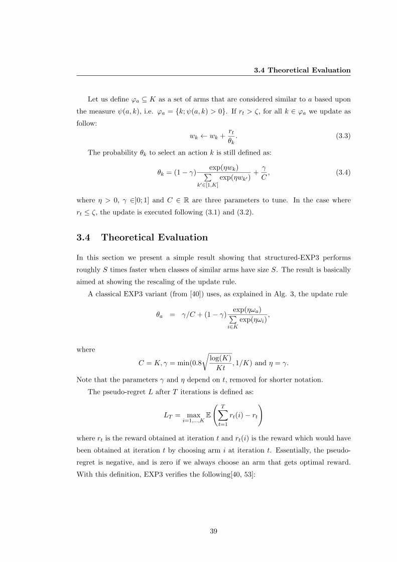
3.4 Theoretical Evaluation
Let us define ϕa ⊆ K as a set of arms that are considered similar to a based upon
the measure ψ(a, k), i.e. ϕa = {k;ψ(a, k) > 0}. If rt > ζ, for all k ∈ ϕa we update as
follow:
wk ← wk +rtθk. (3.3)
The probability θk to select an action k is still defined as:
θk = (1− γ)exp(ηwk)∑
k′∈[1,K]
exp(ηwk′)+γ
C, (3.4)
where η > 0, γ ∈]0; 1] and C ∈ R are three parameters to tune. In the case where
rt ≤ ζ, the update is executed following (3.1) and (3.2).
3.4 Theoretical Evaluation
In this section we present a simple result showing that structured-EXP3 performs
roughly S times faster when classes of similar arms have size S. The result is basically
aimed at showing the rescaling of the update rule.
A classical EXP3 variant (from [40]) uses, as explained in Alg. 3, the update rule
θa = γ/C + (1− γ)exp(ηωa)∑
i∈Kexp(ηωi)
,
where
C = K, γ = min(0.8
√log(K)
Kt, 1/K) and η = γ.
Note that the parameters γ and η depend on t, removed for shorter notation.
The pseudo-regret L after T iterations is defined as:
LT = maxi=1,...,K
E
(T∑t=1
rt(i)− rt
)
where rt is the reward obtained at iteration t and rt(i) is the reward which would have
been obtained at iteration t by choosing arm i at iteration t. Essentially, the pseudo-
regret is negative, and is zero if we always choose an arm that gets optimal reward.
With this definition, EXP3 verifies the following[40, 53]:
39

3. SELECTION POLICY WITH INFORMATION SHARING FORADVERSARIAL BANDIT
Algorithm 3 The EXP3 algorithm as in [40] (left) and TEXP3, sEXP and sTEXP3
variants (right). Strategies are given for player 1. Player 2 use 1− rt instead of rt.
for each iteration t ∈ {1, 2, . . . , T}do
Selection policy π: choose arm a
with probability θa (Eq. 3.4).
Get reward rt.
Update ωa:
wa ← wa +rtθa.
end for
Recommendation: choose arm a with
probability nT (a) = taT .
for each iteration t ∈ {1, 2, . . . , T}do
Selection policy π: choose arm a
with probability θa (Eq. 3.4).
Get reward rt.
Update ωa: wa ← wa + rtθa.
if sEXP3 or sTEXP3 and rt < ζ
then
for each b ∈ ϕ(a) \ a do
wb ← wb +rtθb.
end for
end if
end for
if TEXP3/sTEXP3 then
if ta/T ≤ c then
Set ta = 0.
end if
Rescale ta: ta ← ta/∑
b∈[[1,K]] tb.
end if
Recommendation: choose arm a with
probability nT (a) = taT .
40

3.4 Theoretical Evaluation
Theorem 1: pseudo-regret L of EXP3.
Consider a problem with K arms and 1-sum rewards in [0, 1]. Then, EXP3 verifies
LT ≤ 2.7√TKln(K).
It is known since [49] that it is not possible to do better than the bound above, within
logarithmic factors, in the general case.
We propose a variant, termed Structured-EXP3 or sEXP3, for the case in which for
each arm a, there is a set ϕa (of cardinality S) containing arms similar to a. Under mild
assumptions upon ϕa, the resulting algorithms has some advantages over the baseline
EXP3. The parameters γ and η for sEXP3 are defined by (3.5) and (3.6) respectively
(C = K is preserved, as in EXP3).
γ = min(0.8
√S log(K/S)
Kt, S/K), (3.5)
η = γ/S. (3.6)
In other words, γ is designed (as detailed in the theorem below) for mimicking the values
corresponding to the problem with K/S arms instead of K arms and η is designed for
avoiding a too aggressive pruning.
The following theorem is aimed at showing that parameters in (3.5) and (3.6) ensure
that Structured-EXP3 emulates EXP3 on a bigger problem with a particular structure.
Theorem 2: Structured-EXP3 and pseudo-regret.
Consider a problem where there are K ′ classes of S similar arms i.e. K = K ′ × S(arms from different classes have no similarity); ϕa is the set of arms of the same class
as arm a. Assume that all arms in a class have the same distribution of rewards, i.e.
a ∈ ϕb implies that a and b have the same distribution of rewards against any given
strategy of the opponent. Set ζ = −∞. Then, Structured-EXP3 verifies
LT ≤ 2.7√T (K/S)ln(K/S),
where S is the cardinal of ϕa (whereas the EXP3 bound is 2.7√TKlnK ).
Proof: For this proof, we compare the Structured-EXP3 algorithm with K arms
including classes of S similar arms (i.e. ∀ a ∈ [[1,K]], ϕa = S) and an EXP3 algorithm
working on an ad hoc problem with K/S arms. The ad hoc problem is built as follows.
Instead of arms A = {1, 2, . . . ,K} (ordered by similarity, so that blocks of S
successive arms are similar) for the Structured-EXP3 bandit, consider arms A′ =
41

3. SELECTION POLICY WITH INFORMATION SHARING FORADVERSARIAL BANDIT
{1, S + 1, 2S + 1, . . . ,K − S + 1} for the EXP3 bandit. Consider the same reward
as in the Structured-EXP3 bandit problem.
Any mixed strategy on the EXP3 problem can be transformed without changing
its performance into a mixed strategy on the Structured-EXP3 problem by arbitrarily
distributing the probability of choosing arm i ∈ A′ onto arms {i, i+1, . . . , i+S−1} ⊂ A.
Let us use θ′a′ , the probability that EXP3 chooses a′ ∈ A′; and ω′a′ , the sum of
rewards associated to a′ ∈ A′ for EXP3 (notations with no “prime” are for Structured-
EXP3). We now show by induction that
� ωa = S×ω′a′ for a ∈ A similar to a′ ∈ A′ when EXP3 and Structured-EXP3 have
the same history1;
� θa = 1S θ′a′ for a ∈ A similar to a′ ∈ A′.
The proof is based on the following steps, showing that when the induction properties
hold at some time step then they also hold at the next time step. We assume that
ωa = S×ω′a′ (for all a′ ∈ A′ similar to a) at some iteration, and we show that it implies
θa = 1S θ′a′ at the same iteration (also for all a′ ∈ A′ similar to a) and that ωa = S×ω′a′
at the next iteration (also for all a′ ∈ A′ similar to a). More formally, we show that
∀(a, a′) ∈ A×A′, a ∈ ϕa′ , ωa = S × ω′a′ (3.7)
⇒
∀(a, a′) ∈ A×A′, a ∈ ϕa′ , θa =1
S× θ′a′ (3.8)
and at next iteration (3.7) still holds. The properties of (3.7) and (3.8) hold at the
initial iteration (we have only zeros) and the induction from one step to the next is as
follows:
� Let us show that (3.7) implies (3.8), i.e. if, for all a, ωa for Structured-
EXP3 is S times more than ω′a′ for a′ ∈ A′ similar to a, then the prob-
ability for Structured-EXP3 to choose an arm a ∈ A similar to a′ ∈ A′
is exactly S times less than the probability for EXP3 to choose a′. The
1The set of arms are not the same in Structured-EXP3 and EXP3. By same history we mean up
to the projection a→ a′ = b(a− 1)/Sc+ 1.
42

3.4 Theoretical Evaluation
probability that Structured-EXP3 chooses arm a at iteration t given an history
a1, . . . , at−1 of chosen arms with rewards r1, . . . , rt−1 until iteration t− 1 is
θa = (1− γ)exp(ηwa)∑
k∈[1,K]
exp(ηwk)+γ
K, (3.9)
which is exactly S times less than the probability that EXP3 chooses arm b(a−1)/Sc+1 given a history b(a1−1)/Sc+1, b(a2−1)/Sc+1,. . . ,b(at−1−1)/Sc+1.
Thus,
θa =1
Sθ′a′ .
This is the case because the S additional factor in ωa is compensated by the S
denominator in (3.6) so that terms in the exponential are the same as in the
Structured-EXP3 case; but the numerator is S times bigger. This concludes the
proof that (3.8) holds.
� We now show that the probability that Structured-EXP3 chooses an arm
in {a′, a′+1, . . . , a′+S−1} similar to a′ ∈ A is the same as the probability
that EXP3 chooses a′ ∈ A′ (given the same history). The update rule in
Structured-EXP3 ensures that ωa = ωb as soon as a and b are similar. So the
probability of an arm of the same class as a ∈ A to be chosen by Structured-EXP3
is exactly the probability of a′ ∈ A′ (similar to A) being chosen by EXP3:∑a similar to a′
θa = θ′a′ . (3.10)
� Let us now show that (3.7) and (3.8) implies (3.7) at the next iteration,
i.e. the weighted sum of rewards ωa for a ∈ A is S times more than
the weighted sum of rewards ω′a′ for a similar to a′ (given the same
histories). This is because (i) probabilities that Structured-EXP3 chooses an
arm a among those similar to an arm a′ is the same as the probability that EXP3
chooses a′ (given the same history), as explained by (3.10), and (ii) probabilities
used in the update rule are divided by S in the case of Structured-EXP3 (updates
have K at the denominator). This concludes the induction, from an iteration to
the next.
The induction is complete.
43

3. SELECTION POLICY WITH INFORMATION SHARING FORADVERSARIAL BANDIT
3.5 Experiments
This section describes a set of experiments that evaluates the quality of our approach.
The first testbed is automatically generated sparse matrices and the results are pre-
sented in section 3.5.1. The second testbed, presented in section 3.5.2, is the game
UrbanRivals (UR), an internet card game. Throughout this section, we used 3 base-
lines: EXP3, TEXP3 and Random. The parameters γ, η and C were tuned indepen-
dantly for each testbed (and each algorithm) to ensure they are performing as good as
they can. For the automatically generated sparse matrices, the set of parameters that
gave the best results are η = 1√t, γ = 1√
t, C = 0.65 and α = 0.8. In the game Urban
Rivals, the best values found for the parameters are η = 1√t, γ = 1√
t, C = 0.7 and
α = 0.75.
As a reminder, we add the prefix s when we exploit the notion of distance. The
distance ψ(·, ·) is specific to the testbed and is thus defined in each section.
3.5.1 Artificial experiments
First we test on automatically generated matrices that have a sparse solution and
contain an exploitable measure of distance between the arms. We use matrix M defined
by Mi,j = 12 + 1
5(1 + cos(i× 2× π/100))χi mod ω − 15(1 + cos(j × 2× pi/100))χj mod ω,
where ω ∈ N is set to 5 and M is of size 50 × 50. The distance ψ(·, ·) is based on the
position of the arm in the matrix. It is defined such that the selected arm a and k ∈ Khave a similarity
ψ(a, k) =
{1 if (k′ − a′) mod ω = 0
0 otherwise,(3.11)
where k′ and a′ are the position of respectively k and a in the matrix M . The set ϕa
includes all k where ψ(a, k) = 1. At any t ∈ T the reward is given by the binomial
distribution rt ∼ B(20,M(i, j)), where 20 is the number of Bernoulli trials with pa-
rameter M(i, j). The threshold ζ is fixed at 0.8 and for any given T , the experiment is
repeated 100 times.
Figure 3.1 analyses the score (%) in relation to the maximal number of iterations T
of our approach playing against the baselines. Note that any result over 50% means that
the method wins more often than it looses. Figure 3.1(a) presents the results of sEXP3
and EXP3 playing against the baseline Random. Figure 3.1(b) shows sTEXP3 and
44
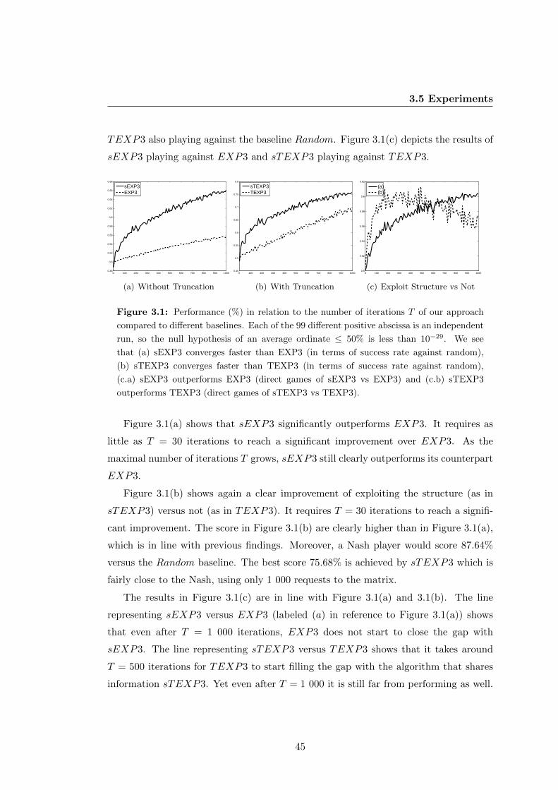
3.5 Experiments
TEXP3 also playing against the baseline Random. Figure 3.1(c) depicts the results of
sEXP3 playing against EXP3 and sTEXP3 playing against TEXP3.
0 100 200 300 400 500 600 700 800 900 10000.48
0.5
0.52
0.54
0.56
0.58
0.6
0.62
0.64
0.66
0.68
sEXP3EXP3
(a) Without Truncation
0 100 200 300 400 500 600 700 800 900 10000.45
0.5
0.55
0.6
0.65
0.7
0.75
0.8
sTEXP3TEXP3
(b) With Truncation
0 100 200 300 400 500 600 700 800 900 10000.5
0.52
0.54
0.56
0.58
0.6
0.62
(a)(b)
(c) Exploit Structure vs Not
Figure 3.1: Performance (%) in relation to the number of iterations T of our approach
compared to different baselines. Each of the 99 different positive abscissa is an independent
run, so the null hypothesis of an average ordinate ≤ 50% is less than 10−29. We see
that (a) sEXP3 converges faster than EXP3 (in terms of success rate against random),
(b) sTEXP3 converges faster than TEXP3 (in terms of success rate against random),
(c.a) sEXP3 outperforms EXP3 (direct games of sEXP3 vs EXP3) and (c.b) sTEXP3
outperforms TEXP3 (direct games of sTEXP3 vs TEXP3).
Figure 3.1(a) shows that sEXP3 significantly outperforms EXP3. It requires as
little as T = 30 iterations to reach a significant improvement over EXP3. As the
maximal number of iterations T grows, sEXP3 still clearly outperforms its counterpart
EXP3.
Figure 3.1(b) shows again a clear improvement of exploiting the structure (as in
sTEXP3) versus not (as in TEXP3). It requires T = 30 iterations to reach a signifi-
cant improvement. The score in Figure 3.1(b) are clearly higher than in Figure 3.1(a),
which is in line with previous findings. Moreover, a Nash player would score 87.64%
versus the Random baseline. The best score 75.68% is achieved by sTEXP3 which is
fairly close to the Nash, using only 1 000 requests to the matrix.
The results in Figure 3.1(c) are in line with Figure 3.1(a) and 3.1(b). The line
representing sEXP3 versus EXP3 (labeled (a) in reference to Figure 3.1(a)) shows
that even after T = 1 000 iterations, EXP3 does not start to close the gap with
sEXP3. The line representing sTEXP3 versus TEXP3 shows that it takes around
T = 500 iterations for TEXP3 to start filling the gap with the algorithm that shares
information sTEXP3. Yet even after T = 1 000 it is still far from performing as well.
45

3. SELECTION POLICY WITH INFORMATION SHARING FORADVERSARIAL BANDIT
Overall for this testbed, the sharing of information greatly increases the performance
of the state-of-the-art algorithms. The good behavior of sparsity techniques such as
TEXP3 is also confirmed.
3.5.2 Urban Rivals
Urban Rivals (UR) is a widely played internet card game, with partial information.
As pointed out in [51], UR can be consistently solved by a Monte-Carlo Tree Search
algorithm (MCTS) thanks to the fact that the hidden information is frequently revealed.
A call for getting a reward leads to 20 games played by a Monte-Carlo Tree Search with
1 000 simulations before an action is chosen.
Reading coefficients in the payoff matrices at the root is quite expensive, and we
have to solve the game approximately.
We consider a setting in which two players choose 4 cards from a finite set of 10
cards. We use two different representations. In the first one, each arms a ∈ K is
a combinations of 4 cards and K = 104. In the second representation, we remove
redundant arms. There remain K = 715 different possible combinations if we allow the
same card to be used more than once in the same combination.
There are two baseline methods tested upon UR, namely EXP3 and TEXP3.
The distance ψ(·, ·) is based on the number of similar cards. It is defined such that
the selected arm a and k ∈ K have a distance
ψ(a, k) =
{1 if k and a share more than 2 cards
0 otherwise,(3.12)
The set ϕa includes all k where ψ(a, k) = 1. At any t ≤ T the reward rt is given by 20
games played with the given combinations. The threshold ζ is fixed at 0.8 and for any
given T .
For a given number of iterations T , each algorithm is executed 10 times and the
output is saved. To compute the values in Figure 3.2, we play a round-robin (thus
comparing 10 × 10 different outputs) where each comparison between two outputs
consist in repeating 100 times the process of selecting an arm and executing 20 games.
Figure 3.2 presents the score (%) in relation to the maximal number of iterations
T of our approach playing against their respective baselines. Figure 3.2(a) presents
the results of sEXP3 playing against EXP3. Figure 3.2(b) shows sTEXP3 playing
46

3.5 Experiments
against TEXP3. In both cases, we present the results for 2 different representations
(K = 104, and K = 715).
100 200 300 400 500 600 700 800 900 10000.55
0.56
0.57
0.58
0.59
0.6
0.61
0.62
0.63
0.64
0.65
K = 104
K = 715
(a) sEXP3 vs EXP3
100 200 300 400 500 600 700 800 900 1000
0.58
0.59
0.6
0.61
0.62
0.63
0.64
0.65
0.66
0.67
K = 104
K = 715
(b) sTEXP3 vs TEXP3
Figure 3.2: Performance (%) in relation to the number of iterations T of our approach
compared to different baselines. Standard deviations are smaller than 1%. We see that
(a) sEXP3 outperforms EXP3 in both versions (game with 10K arms and game with 715
arms) (b) sTEXP3 outperforms TEXP3 in both versions (game with 10K arms and game
with 715 arms).
Figure 3.2(a) shows that sEXP3 significantly outperforms EXP3 independently
of the representation since the values are far beyond 50%. Even at the lowest number
of iterations (T = 100), there is a significant improvement over EXP3 with both
representations (K = 104 and K = 715). As the maximal number of iterations T grows,
sEXP3 still clearly outperforms its counterpart EXP3. Moreover, Figure 3.2(a) shows
that the representation impacts greatly on the quality of the results. The discrepancy
between the two lines is probably closely related to the ratio TK . For instance, when
T = 1 000 and K = 104 the score is equal to 60.88%. If we compare such a result to
T = 100 and K = 715, a ratio TK relatively close, the score (60.22%) is rather similar.
Figure 3.2(b) shows that sTEXP3 significantly outperforms TEXP3 independently
of the representation since the values are also far beyond 50%. The conclusion drawn
from Figure 3.2(b) are quite similar to the ones from Figure 3.2(a). However, the
sudden drop at T = 1 000 and K = 715 indicates that TEXP3 also start to converge
toward the Nash Equilibrium, thus bringing the score relatively closer to the 50% mark.
47

3. SELECTION POLICY WITH INFORMATION SHARING FORADVERSARIAL BANDIT
For the game UR, it seems that sharing information does also greatly improve the
performance of the state-of-the-art algorithms.
3.6 Conclusion
In this chapter, we present an improvement over state-of-the-art algorithms to compute
an ε-approximation of a Nash Equilibrium for zero-sum matrix games. The improve-
ment consists in exploiting the similarities between arms of a bandit problem through
a notion of distance and in sharing information among them.
From a theoretical point of view, we compute a bound for our algorithm that is
better then the state-of-the-art by a factor roughly based on the number of similar
arms. The sparsity assumption is not a necessity to ensure convergence, it simply
ensure faster convergence.
Moreover, empirical results on the game of Urban Rival and automatically generated
matrices with sparse solutions show a significant better performance of the algorithms
that share information compared to the ones that do not. This is when results are
compared on the basis of EXP3 parameters that are optimized on the application.
As future work, the next step is to create a parameter free version of our algorithm,
for instance by automatically fixing the parameter ζ. Also, so far we solely focus on
problem where the total number of iterations T is too small for converging to the NE.
As the maximal number of iterations T gets bigger, there would be no reason for sharing
information anymore. A degradation function can be embedded into the updating rule
to ensure convergence. We do not know for the moment whether we should stop sharing
information depending on rewards (using ζ), depending on iterations (using a limit on
t/T ) or more sophisticated criteria.
48

4
Simulation Policy for Symbolic
Regression
4.1 Introduction
In this chapter, we study the simulation policy. The reason to seek an improvement over
the simulation policy is rather straightforward. A more efficient sampling of a space
requires less samples to find a solution. Simulation policy is considered essentially, albeit
not exclusively, domain specific or problem dependent. It means that an improvement
of the simulation policy for a given problem may not be adequate for another one. A
modification in such policy can be tricky when embedded into a MCS algorithms. For
instance, it can either prevent the algorithm to converge to a solution or converge to
the wrong one.
Lets take the game of Go as an example, where the best algorithms are mainly
MCTS. It was repeatedly shown that the use of stronger simulation policies can lead
to weaker MCS algorithms [54, 55]. It is mainly related to the fact that a modification
of the simulation policy is introducing a bias in the probability distribution to exploit
specific knowledge [56]. By doing so, one can basically increase its winning probability
against a specific opponent while moving further away from the optimal solution. It
is thus important to focus on improving a simulation policy embedded into a MCS
algorithms rather than simply improving the simulation policy alone.
For our discussion on the work done over the simulation policy, we focus on a specific
problem that is commonly labeled Symbolic Regression. This problem was chosen over
49
4. SIMULATION POLICY FOR SYMBOLIC REGRESSION
several others because it has two main advantages. First, Symbolic Regression is well-
known and has potential applications in many different fields. Thus, a finding on this
problem is relevant to many. Second, Symbolic Regression is essentially finding an
expression that best represents an input. It is not far-fetched to imagine that such a
work can be used to build our own selection policy as it was done in [38, 57] or even
customize our own MCS algorithm [58].
In the following, Section 4.2 introduces more specifically the notion of Symbolic
Regression and Section 4.3 formalizes the problem. Section 4.4 describes the proposed
approach to modify the probabilities inside a set. Section 4.5 present the notion of
partitionning the problem into smaller ones and computes several sets of probabilities.
Section 4.5 describes such an approach. Section 4.6 explains the resulting learning
algorithm. Section 4.7 presents the experimental results and Section 4.8 concludes on
the chapter.
4.2 Symbolic Regression
A large number of problems can be formalized as finding the best expressions, or
more generally the best programs, to maximize a given numerical objective. Such
optimization problems over expression spaces arise in the fields of robotics [59], finance
[60], molecular biology [61], pattern recognition [62], simulation and modeling [63] or
engineering design [64] to name a few.
These optimization problems are hard to solve as they typically involve very large
discrete spaces and possess few easily exploitable regularities, mainly due to the com-
plexity of the mapping from an expression syntax to its semantic (e.g. the expressions
c× (a+ b) and c/(a+ b) differ only by one symbol but have totally different semantics).
Due to the inherent difficulties related to the nature of expression spaces, these
optimization problems can rarely be solved exactly and a wide range of approximate
optimization techniques based on stochastic search have been proposed. In particular, a
large body of work has been devoted to evolutionary approaches known as genetic pro-
gramming [65, 66, 67]. While genetic programming algorithms have successfully solved
a wide range of real-world problems, these algorithms may be complex to implement
and are often too difficult to analyze from a theoretical perspective.
50

4.3 Problem Formalization
[68] recently proposed to use a search technique based on Monte-Carlo sampling to
solve optimization problems over expression spaces, a promising alternative approach
that avoids some important pitfalls of genetic programming. One key component of
this Monte-Carlo approach is the procedure that samples expressions randomly. The
proposed approach was based on uniformly sampling expression symbols. This choice
fails to tackle the redundancy of expressions: it is often the case that a large number
of syntactically different expressions are equivalent, for example due to commutativity,
distributivity or associativity. This choice also does not take into account that some
expressions may have an undefined semantic, due to invalid operations such as division
by zero.
In this chapter we focus on the two improvements. First, an improvement of the
sampling procedure used in the context of Monte Carlo search over expression spaces
[69]. Given a number T of trials, we want to determine a memory-less sampling proce-
dure maximizing the expected number of semantically different valid expressions gen-
erated ST ≤ T . To reach this objective, we propose a learning algorithm which takes
as input the available constants, variables and operators and optimizes the set of sym-
bol probabilities used within the sampling procedure. We show that, on medium-scale
problems, the optimization of symbol probabilities significantly increases the number
of non-equivalent expressions generated. For larger problems, the optimization prob-
lem cannot be solved exactly. However, we show empirically that solutions found on
smaller problems can be used on larger problems while still significantly outperforming
the default uniform sampling strategy.
Second, we build on this work and further enhance the sampling methods by con-
sidering several different sets of parameters to generate expressions [70]. In order to
obtain these different sets, we provide a method that first partition the samples into
different subsets, then apply a learning algorithm that computes a probability distri-
bution on each cluster. The sheer number of different expressions generated increases
compared to both the uniform sampling [68] and the one in [69].
4.3 Problem Formalization
We now introduce Reverse Polish Notation (RPN) as a way of representing expressions
in Section 4.3.1 and describe a generative process compliant with this representation
51

4. SIMULATION POLICY FOR SYMBOLIC REGRESSION
Algorithm 4 RPN evaluation
Require: s ∈ AD: a sequence of length D
Require: x ∈ X: variable values
stack ← ∅for d = 1 to D do
if αd is a variable or a constant then
Push the value of αd onto the stack.
else
Let n be the arity of operator αd.
if |stack| < n then
syntax error
else
Pop the top n values from the stack, compute αd with these operands, and
push the result onto the stack.
end if
end if
end for
if |stack| 6= 1 then
syntax error
else
return top(stack)
end if
in Section 4.3.2. Section 4.3.3 carefully states the problem addressed in this chapter.
4.3.1 Reverse polish notation
RPN is a representation wherein every operator follows all of its operands. For in-
stance, the RPN representation of the expression c× (a+ b) is the sequence of symbols
[c, a, b,+,×]. This way of representing expressions is also known as postfix notation
and is parenthesis-free as long as operator arities are fixed, which makes it simpler to
manipulate than its counterparts, prefix notation and infix notation.
Let A be the set of symbols composed of constants, variables and operators. A
sequence s is a finite sequence of symbols of A: s = [α1, . . . , αD] ∈ A∗. The evaluation
of an RPN sequence relies on a stack and is depicted in Algorithm 4. This evaluation
fails either if the stack does not contain enough operands when an operator is used or if
52

4.3 Problem Formalization
Table 4.1: Size of UD, ED and AD for different sequence lengths D.
D |UD| |ED| |UD||ED|% |AD| |ED|
|AD|%
1 4 4 100 11 36.4
2 20 28 71.4 121 23.1
3 107 260 41.2 1331 19.5
4 556 2 460 22.6 14 641 16.8
5 3 139 24 319 12.9 161 051 15.1
6 18 966 244 299 7.8 1 771 561 13.8
7 115 841 2 490 461 4.7 19 487 171 12.8
the stack contains more than one single element at the end of the process. The sequence
[a,×] leads to the first kind of errors: the operator × of arity 2 is applied with a single
operand. The sequence [a, a, a] leads to the second kind of errors: evaluation finishes
with three different elements on the stack. Sequences that avoid these two errors are
syntactically correct RPN expressions and are denoted e ∈ E ⊂ A∗.
Let X denote the set of admissible values for the variables of the problem. We
denote e(x) the outcome of Algorithm 4 when used with expression e and variable
values x ∈ X. Two expressions e1 ∈ E and e2 ∈ E are semantically equivalent if
∀x ∈ X, e1(x) = e2(x). We denote this equivalence relation e1 ∼ e2. The set of
semantically incorrect expressions I ⊂ E is composed of all expressions e for which
there exists x ∈ X such that e(x) is undefined, due to an invalid operation such as
division by zero or logarithm of a negative number. In the context of Monte-Carlo
search, we are interested in sampling expressions that are semantically correct and
semantically different. We denote U = (E − I)/ ∼ the quotient space of semantically
correct expressions by relation ∼. One element u ∈ U is an equivalence class which
contains semantically equivalent expressions e ∈ u.
We denote AD (resp. ED and UD) the set of sequences (resp. expressions and
equivalence classes) of length D. Table 4.1 presents the cardinality of these sets for
different lengths D with a hypothetical alphabet containing four variables, three unary
operators and four binary operators: A = {a, b, c, d, log ,√·, inv,+,−,×,÷}, where inv
stands for inverse. It can be seen that both the ratio between |ED| and |AD| and the
ratio between |UD| and |ED| decrease when increasing D. In other terms, when D
gets larger, finding semantically correct and different expressions becomes harder and
53

4. SIMULATION POLICY FOR SYMBOLIC REGRESSION
Table 4.2: Set of valid symbols depending on the current state. Symbols are classified
into C onstants, V ariables, U nary operators and B inary operators
State Valid symbols
|stack| = 0 C,V
|stack| = 1 & d < D − 1 C,V,U
|stack| = 1 & d = D − 1 U
|stack| ∈ [2, D − d[ C,V,U,B
|stack| = D − d U,B
|stack| = D − d+ 1 B
harder, which is an essential motivation of this work.
4.3.2 Generative process to sample expressions
Monte-Carlo search relies on a sequential generative process to sample expressions e ∈ED. We denote by P [αd|α1, . . . , αd−1] the probability to sample symbol αd after having
sampled the (sub)sequence α1, . . . , αd−1. The probability of an expression e ∈ ED is
then given by:
PD[e] =D∏d=1
P [αd|α1, . . . , αd−1]. (4.1)
An easy way to exclude syntactically incorrect sequences is to forbid symbols that
could lead to one of the two syntax errors described earlier. This leads to a set of
conditions on the current state of the stack and on the current depth d that Table 4.2
summarizes for a problem with variables, constants, unary and binary operators. As it
can be seen, conditions can be grouped into a finite number of states, 6 in this case. In
the following, we denote S the set of these states, we use the notation s(α1, . . . , αd) ∈ S
to refer to the current state reached after having evaluated α1, . . . , αd and we denote
As ⊂ A the set of symbols which are valid in state s ∈ S.
The default choice when using Monte-Carlo search techniques consists in using a
uniformly random policy. Combined with the conditions to generate only syntactically
correct expressions, this corresponds to the following probability distribution:
P [αd|α1, . . . , αd−1] =
{1|As| if αd ∈ As
0 otherwise,(4.2)
54
4.3 Problem Formalization
with s = s(α1, . . . , αd−1).
Note that the sampling procedure described above generates expressions of size
exactly D. If required, a simple trick can be used to generate expressions of size between
1 and D: it consists in using a unary identity operator that returns its operand with
no modifications. An expression of size d < D can then be generated by selecting
αd+1 = · · · = αD = identity.
4.3.3 Problem statement
Using a uniformly random strategy to sample expressions does neither take into account
redundancy nor semantic invalidity. We therefore propose to optimize the sampling
strategy, to maximize the number of valid, semantically different, generated expressions.
Given a budget of T trials, a good sampling strategy should maximize ST , the num-
ber of semantically different, valid generated expressions, i.e. the number of distinct
elements drawn from UD. A simple approach therefore would be to use a rejection sam-
pling algorithm. In order to sample an expression, such an approach would repeatedly
use the uniformly random strategy until sampling a valid expression that differs from
all previously sampled expressions in the sense of ∼. However, this would quickly be
impractical: in order to sample T expressions, such an approach requires memorizing T
expressions, which can quickly saturate memory. Furthermore, in regards of the results
of Table 4.1, the number of trials required within the rejection sampling loop could
quickly grow.
In order to avoid the excessive CPU and RAM requirements of rejection sampling,
and consistently with the definitions given previously, we focus on a distribution PD[e]
which is memory-less. In other terms, we want a procedure that generates i.i.d. ex-
pressions. In addition to the fact that it requires only limited CPU and RAM, such
a memory-less sampling scheme has another crucial advantage: its implementation
requires no communication, which makes it particularly adapted to (massively) paral-
lelized algorithms.
In summary, given the alphabet A, a target depth D and a target number of trials
T , the problem addressed in this chapter consists in finding the distribution PD[·] ∈ P
such that:
P = argmaxP∈P
E{ST }, (4.3)
55

4. SIMULATION POLICY FOR SYMBOLIC REGRESSION
where ST is the number of semantically different valid expressions generated using the
generative procedure PD[·] defined by P .
4.4 Probability set learning
We now describe our approach to learn a sampling strategy taking into account redun-
dant and invalid expressions. Section 4.4.1 reformulates the problem and introduces two
approximate objective functions with good numerical properties. Section 4.4.2 focuses
on the case where the sampling strategy only depends on the current state of the stack
and depth. Finally, the proposed projected gradient descent algorithm is described in
Section 4.4.3.
4.4.1 Objective reformulation
Let PD[u] be the probability to draw any member of the equivalence class u:
PD[u] =∑e∈u
PD[e] (4.4)
The following lemma shows how to calculate the expectation of obtaining at least one
member of a given equivalence class u after T trials.
Lemma 4.1 Let Xu be a discrete random variable such that Xu = 1 if u is generated
after T trials and Xu = 0 otherwise. The probability to generate at least once u over T
trials is equal to
E{Xu} = 1− (1− PD[u])T . (4.5)
Proof Since at each trial the probability for u ∈ U to be generated does not depend on
the previous trials, the probability over T trials that Xu = 0 is given by (1− PD[u])T .
Thus, the probability that Xu = 1 is its complementary and given by 1− (1−PD[u])T .
We now aggregate the different random variables.
Lemma 4.2 The expectation of the number TS of different equivalence classes u gen-
erated after T trials is equal to
E{TS} =∑u∈UD
1− (1− PD[u])T . (4.6)
56
4.4 Probability set learning
Proof This follows from E{∑u∈UD
Xu} =∑u∈UD
E{Xu}.
Unfortunately, in the perspective of a using gradient descent optimization scheme,
the formula given by Lemma 4.2 is numerically unstable. Typically, PD[u] is very
small and the value (1− PD[u])T has a small number of significant digits. This causes
numerical instabilities that become particularly problematic as T and |U| increase.
Therefore, we have to look for an approximation of (4.6) that has better numerical
properties.
Lemma 4.3 For 0 < PD[u] < 1T , using the Newton Binomial Theorem to compute
1− (1− PD[u])T , the terms are decreasing.
Proof Using the Newton Binomial Theorem, (4.5) reads
1− (1− PD[u])T = 1−T∑k=0
(Tk
)(−PD[u])k
=
(T1
)(−PD[u]) +
(T2
)(−PD[u])2
+ · · ·+ (−PD[u])T . (4.7)
If PD[u] is sufficiently small, the first term in (4.7) is the biggest. In particular, if
PD[u] < 1T , we claim that
(T0
)PD[u]0 >
(T1
)PD[u]1 >(
T2
)PD[u]2 > · · · >
(Tn
)PD[u]n
As a proof, considering n ∈ {1, 2, . . . , T}, we have to check that
(Tn
)PD[u]n <
(T
n− 1
)PD[u]n−1
⇔ T !
n!(T − n)!PD[u]n <
T !
(n− 1)!(T − n+ 1)!PD[u]n−1
⇔ PD[u] <n
T − n+ 1(4.8)
(4.8) holds when 0 < PD[u] < 1T , n ≥ 1 and T ≥ 0.
Observation 1 For 0 < PD[u] < 1λT , two successive terms in the Newton Binomial
Theorem decrease by a coefficient of 1λ .
57
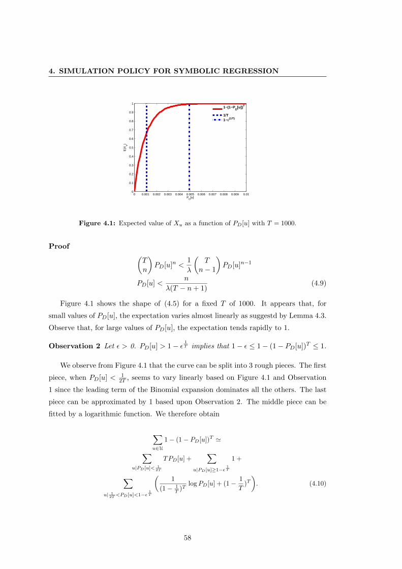
4. SIMULATION POLICY FOR SYMBOLIC REGRESSION
0 0.001 0.002 0.003 0.004 0.005 0.006 0.007 0.008 0.009 0.010
0.1
0.2
0.3
0.4
0.5
0.6
0.7
0.8
0.9
1
PD
[u]
E(X
u)
1−(1−P
D[u]) T
1/T1−ε(1/T)
Figure 4.1: Expected value of Xu as a function of PD[u] with T = 1000.
Proof (Tn
)PD[u]n <
1
λ
(T
n− 1
)PD[u]n−1
PD[u] <n
λ(T − n+ 1)(4.9)
Figure 4.1 shows the shape of (4.5) for a fixed T of 1000. It appears that, for
small values of PD[u], the expectation varies almost linearly as suggestd by Lemma 4.3.
Observe that, for large values of PD[u], the expectation tends rapidly to 1.
Observation 2 Let ε > 0. PD[u] > 1− ε1T implies that 1− ε ≤ 1− (1− PD[u])T ≤ 1.
We observe from Figure 4.1 that the curve can be split into 3 rough pieces. The first
piece, when PD[u] < 12T , seems to vary linearly based on Figure 4.1 and Observation
1 since the leading term of the Binomial expansion dominates all the others. The last
piece can be approximated by 1 based upon Observation 2. The middle piece can be
fitted by a logarithmic function. We therefore obtain
∑u∈U
1− (1− PD[u])T '∑u|PD[u]< 1
2T
TPD[u] +∑
u|PD[u]≥1−ε1T
1 +
∑u| 1
2T <PD[u]<1−ε1T
(1
(1− 1T )T
logPD[u] + (1− 1
T)T). (4.10)
58
4.4 Probability set learning
An even rougher approach could be to consider only two pieces and write (4.6),
using Lemma 4.3 and Observation 2 as
∑u∈U
1− (1− PD[u])T '∑u|PD[u]< 1
T
TPD[u] +∑
u|PD[u]≥ 1T
1. (4.11)
4.4.2 Instantiation and gradient computation
In this section, we focus on a simple family of probability distributions with the as-
sumption that the probability of a symbol only depends on the current state s ∈ S and
is otherwise independent of the full history α1, . . . , αd−1. We thus have:
PD[e] =D∏d=1
P [αd|s(α1, . . . , αd−1)]. (4.12)
In the following, we denote {ps,α} the set of probabilities, such that P [α|s] = ps,α
for all s ∈ S and α ∈ As.
Our objective is to optimize (4.10) or (4.11) subject to∑α∈As
ps,α = 1 for all s ∈ S
and the nonnegative constraint ps,α > 0 for all s ∈ S and α ∈ As.
Observe that the gradient is easy to compute for both objectives. We detail here
the gradient when (4.11) is used as the objective function.
Lemma 4.4 The derivative ∂(·)∂ps,α
of (4.11) is given by
T∑
u|PD[u]< 1T
∑e∈u
ns,α(e)PD[e],
where ns,α(e) is the number of times the symbol α ∈ As is used from state s ∈ S when
generating e.
59

4. SIMULATION POLICY FOR SYMBOLIC REGRESSION
Proof
∂f
∂ps,α=
∂
∂ps,α(
∑u|PD[u]< 1
T
TPD[u] +∑
u|PD[u]≥ 1T
1 )
=∂
∂ps,α(T
∑u|PD[u]< 1
T
∑e∈u
PD[e] )
= T∑
u|PD[u]< 1T
∑e∈u
∂
∂ps,α(
∏s,α|ns,α(e)>0
pns,αs,α )
Note that this objective function is not convex. However, empirical experiments
show that it is rather easy to optimize and that obtained solutions are robust w.r.t. to
choice of the starting point of the gradient descent algorithm.
4.4.3 Proposed algorithm
We propose to use a classical projected gradient descent algorithm to solve the opti-
mization problem described previously. Algorithm 5 depicts our approach. Given the
symbol alphabet A, the target depth D and the target number of trials T , the algorithm
proceeds in two steps. First, it constructs an approximated set UD by discriminating
the expressions on the basis of random samples of the input variables, following the
procedure detailed below. It then applies projected gradient descent, starting from
uniform ps,α probabilities and iterating until some stopping conditions are reached.
To evaluate approximately whether e1 ∼ e2, we compare e1(x) and e2(x) using a
finite amount X of samples x ∈ X. If the results of both evaluations are equal on
all the samples, then the expressions are considered as semantically equivalent. If the
evaluation fails for any of the samples, the corresponding expression is considered as
semantically incorrect and is rejected. Empirical tests showed that with as little as
X = 5 samples, more than 99% of U was identified correctly for D ranging in [1, 8].
With X = 100 samples the procedure was almost perfect.
The complexity of Algorithm 5 is linear in the size of ED. In practice, only a few
tens iterations of gradient descent are necessary to reach convergence and most of the
computing time is taken by the construction of U. The requirement that the set ED
can be exhaustively enumerated is rather restrictive, since it limits the applicability
of the algorithm to medium values of D. Nevertheless, we show in Section 4.7 that
60

4.4 Probability set learning
Algorithm 5 Symbol probabilities learning
Require: Alphabet A,
Require: Target depth D,
Require: Target budget T ,
Require: A set of input samples x1, . . . , xX
U← ∅for e ∈ ED do
if ∀i ∈ [1, X], e(xi) is well-defined then
Add e to U using key k = {e(x1), . . . , e(xX)}end if
end for
Initialize: ∀s ∈ S, ∀α ∈ As, ps,α ← 1|As|
repeat
∀s ∈ S, ∀α ∈ As, gs,α ← 0
for each u ∈ U with PD[u] < 1T do
for each e ∈ u do
for each s ∈ S, α ∈ As with ns,α(e) > 0 do
gs,α ← gs,α + ns,α(e)PD[e]
end for
end for
end for
Apply gradient gs,α and renormalize ps,α
until some stopping condition is reached
return {ps,α}
61

4. SIMULATION POLICY FOR SYMBOLIC REGRESSION
probabilities learned for a medium value of D can be used for larger-scale problems
and still significantly outperform uniform probabilities.
4.5 Combination of generative procedures
In Section 4.4, we propose a technique that, given the complete set of unique expressions
of a given depth, is able to compute an optimal set of parameters that maximizes
the expectation of the number of different expressions generated after T trials. The
main drawback of the method is that it needs to have the complete description of all
expressions in order to be able to compute the set of optimal parameters. This is
however computationally prohibitive to enumerate when the depth of the considered
expressions becomes large. There are two alternatives proposed in [69]. The first
alternative is to extrapolate the sets of parameters obtained for a low depth to a larger
depth. The second alternative is to uniformly sample the expressions, identify identical
expressions and optimize the parameters of the distributions P (α|S) used to generate
expressions (see section 4.3.2), based on the expressions sampled and using a gradient-
descent upon the objective defined by
∑u|PD[u]< 1
T
TPD[u] +∑
u|PD[u]≥ 1T
1. (4.13)
In this section, we investigate the possibility to use a combination of generative
procedures rather than a single one. In other words, we propose to deviate from the
idea of selecting only one set of parameters throughout T trials. Instead, we show
analytically that using different sets of parameters can increase E{ST }, the expected
number of different valid expressions generated. We compare the two strategies to
generate expressions.
Both processes start by generating E, a set of initial expressions by uniform sam-
pling. The first process consists in optimizing a single set of parameters as suggested by
[69]. We make T trials with the optimized static set of parameters and every expression
e has a probability pe of being drawn in one trial t.
In the second process, we partition the expressions e ∈ E into K clusters (the
practical procedure is described in Section 4.6) and, for each cluster Ck∈K , we optimize
a distinct set of parameters using only e ∈ E ∩ Ck, the expressions in that cluster.
62

4.5 Combination of generative procedures
Although we consider only a small subset of the complete list of expressions, we aim
with such a procedure at considering very different sets of parameters. In particular,
by maximizing the expected number of different expressions of a given small subset,
we hope that a superset of the expressions considered for the optimization problem see
their overall probability of being generated increased by a small value δ. This should be
the case for all expressions that are sufficiently syntactically similar to those considered
in the cluster. In the same time, some other expressions see their overall probability
decrease by a small value ε. This should consist of expressions that are syntactically
different from those considered in the cluster.
From a theoretical point of view, we can justify this idea with a toy example.
Imagine a set of 2 expressions {e1, e2} and a number of trials T = 2. In the first case,
we place ourselves in a perfect situation where they both have a probability of being
generated of 50%. The expectancy is 1.5 (2 × 0.5 + 1 × 0.5). In the second, we use 2
different sets of parameters, one for each trial. In the first set, the parameters are {1, 0}and in the second they are equal to {0, 1}. This time, the expectancy is 2. Obviously
this is a rather extreme example, but the core idea is clearly presented.
Note that the cluster C0 contains all expressions whose individual probability pe is
large enough (pe >1T ) such that the probability of drawing an expression e ∈ C0 at
least once after T trials is close to 1. These expressions do not require any attention
and therefore we only discuss expressions in clusters C1, . . . , CK , expressions that have
a relatively low probability pe <1T of being drawn.
We assume that, during the T ′ < T2 first trials, the probability of every expression
in Ck increases by δ, thus becoming pe + δ. Moreover, to simplify the analysis, let us
also assume that every expression in Ck has its probability decreased by ε = δ during
T ′ other trials.
We will now prove that the expectation of the random variable
Xqe =
{1 if expression e is drawn at least once
0 otherwise,(4.14)
where q = 1 represents the first process and q = 2 represents the second process,
increases in the second process for all expressions in clusters C1, . . . , Ck compared to
the first process. The expectation of expressions e ∈ C0 is trivially equal in both
processes. We now compare the expectation in the two processes.
63
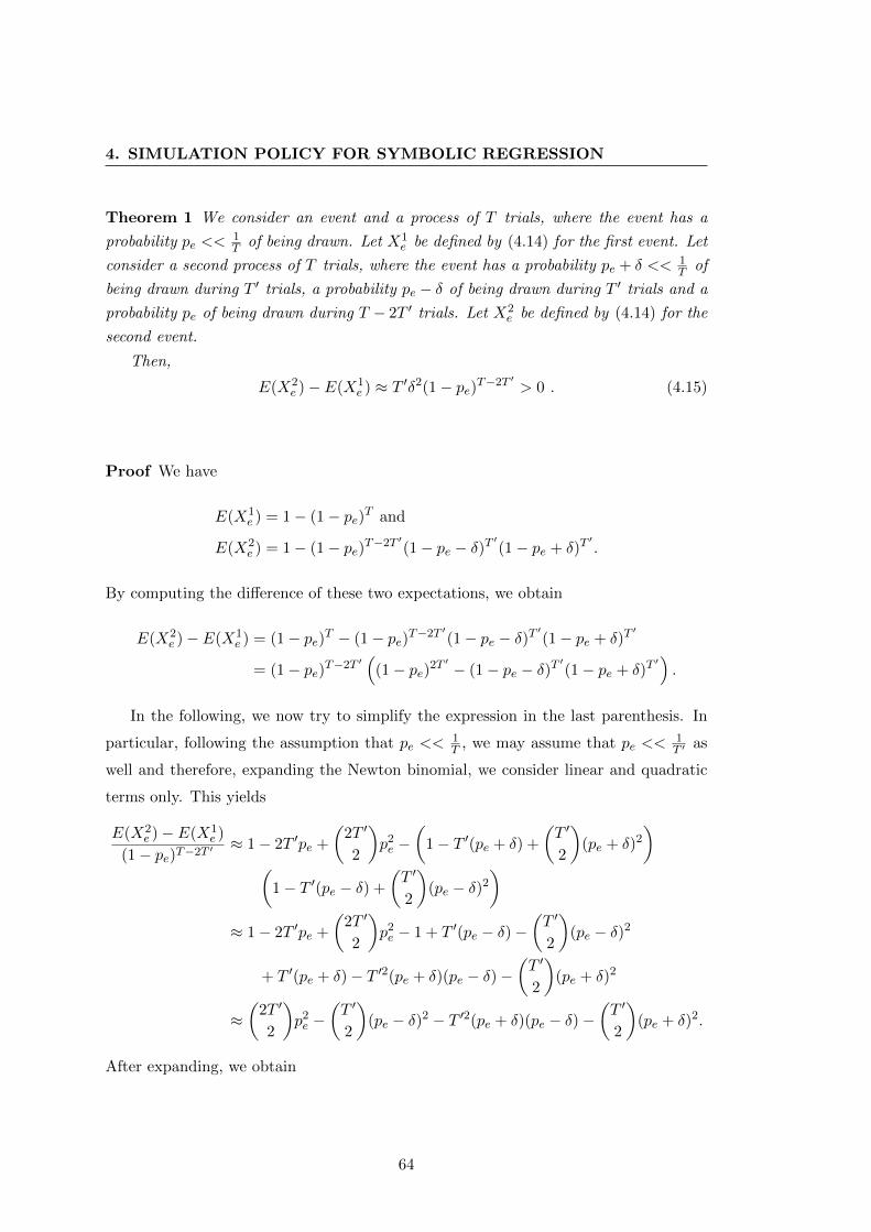
4. SIMULATION POLICY FOR SYMBOLIC REGRESSION
Theorem 1 We consider an event and a process of T trials, where the event has a
probability pe <<1T of being drawn. Let X1
e be defined by (4.14) for the first event. Let
consider a second process of T trials, where the event has a probability pe + δ << 1T of
being drawn during T ′ trials, a probability pe − δ of being drawn during T ′ trials and a
probability pe of being drawn during T − 2T ′ trials. Let X2e be defined by (4.14) for the
second event.
Then,
E(X2e )− E(X1
e ) ≈ T ′δ2(1− pe)T−2T ′ > 0 . (4.15)
Proof We have
E(X1e ) = 1− (1− pe)T and
E(X2e ) = 1− (1− pe)T−2T ′(1− pe − δ)T
′(1− pe + δ)T
′.
By computing the difference of these two expectations, we obtain
E(X2e )− E(X1
e ) = (1− pe)T − (1− pe)T−2T ′(1− pe − δ)T′(1− pe + δ)T
′
= (1− pe)T−2T ′(
(1− pe)2T ′ − (1− pe − δ)T′(1− pe + δ)T
′).
In the following, we now try to simplify the expression in the last parenthesis. In
particular, following the assumption that pe <<1T , we may assume that pe <<
1T ′ as
well and therefore, expanding the Newton binomial, we consider linear and quadratic
terms only. This yields
E(X2e )− E(X1
e )
(1− pe)T−2T ′≈ 1− 2T ′pe +
(2T ′
2
)p2e −
(1− T ′(pe + δ) +
(T ′
2
)(pe + δ)2
)(
1− T ′(pe − δ) +
(T ′
2
)(pe − δ)2
)≈ 1− 2T ′pe +
(2T ′
2
)p2e − 1 + T ′(pe − δ)−
(T ′
2
)(pe − δ)2
+ T ′(pe + δ)− T ′2(pe + δ)(pe − δ)−(T ′
2
)(pe + δ)2
≈(
2T ′
2
)p2e −
(T ′
2
)(pe − δ)2 − T ′2(pe + δ)(pe − δ)−
(T ′
2
)(pe + δ)2.
After expanding, we obtain
64
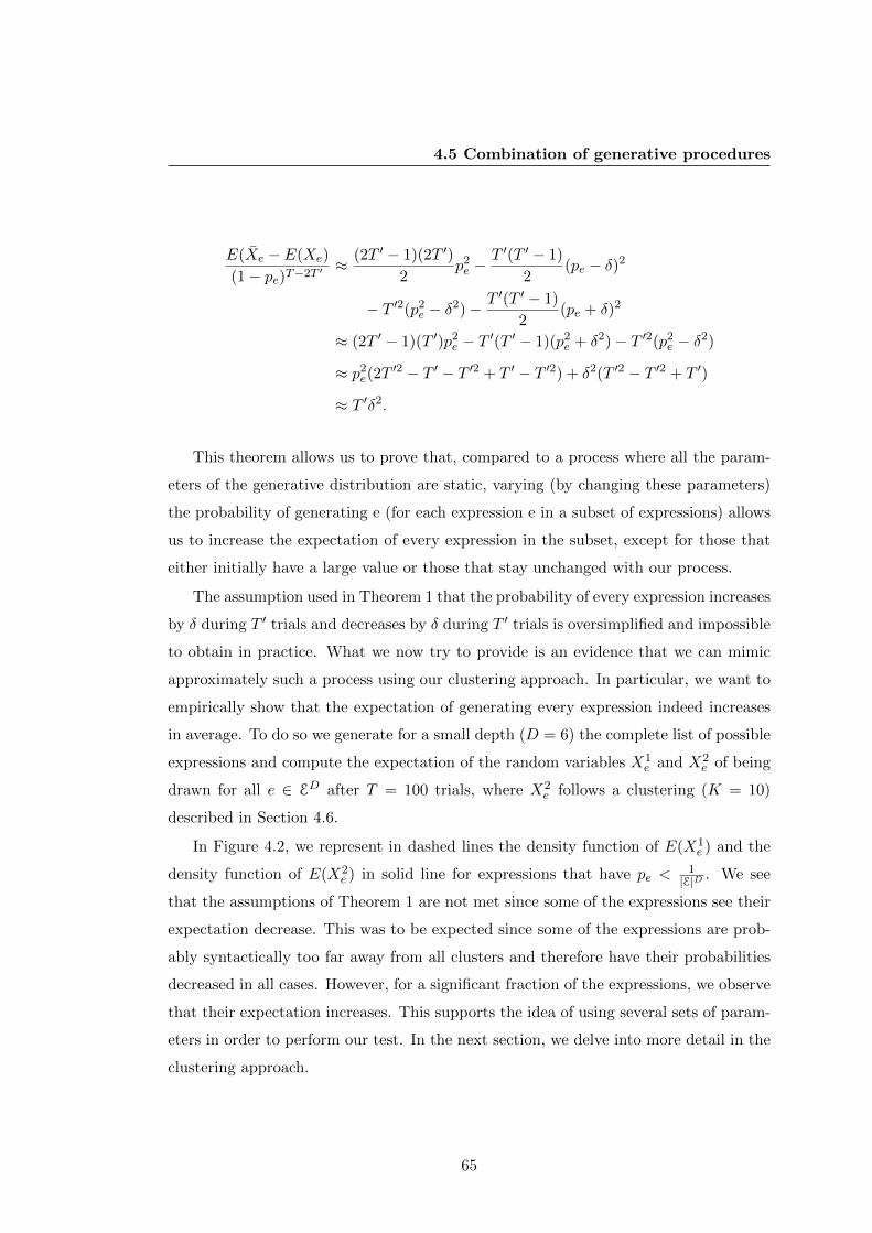
4.5 Combination of generative procedures
E(Xe − E(Xe)
(1− pe)T−2T ′≈ (2T ′ − 1)(2T ′)
2p2e −
T ′(T ′ − 1)
2(pe − δ)2
− T ′2(p2e − δ2)− T ′(T ′ − 1)
2(pe + δ)2
≈ (2T ′ − 1)(T ′)p2e − T ′(T ′ − 1)(p2
e + δ2)− T ′2(p2e − δ2)
≈ p2e(2T
′2 − T ′ − T ′2 + T ′ − T ′2) + δ2(T ′2 − T ′2 + T ′)
≈ T ′δ2.
This theorem allows us to prove that, compared to a process where all the param-
eters of the generative distribution are static, varying (by changing these parameters)
the probability of generating e (for each expression e in a subset of expressions) allows
us to increase the expectation of every expression in the subset, except for those that
either initially have a large value or those that stay unchanged with our process.
The assumption used in Theorem 1 that the probability of every expression increases
by δ during T ′ trials and decreases by δ during T ′ trials is oversimplified and impossible
to obtain in practice. What we now try to provide is an evidence that we can mimic
approximately such a process using our clustering approach. In particular, we want to
empirically show that the expectation of generating every expression indeed increases
in average. To do so we generate for a small depth (D = 6) the complete list of possible
expressions and compute the expectation of the random variables X1e and X2
e of being
drawn for all e ∈ ED after T = 100 trials, where X2e follows a clustering (K = 10)
described in Section 4.6.
In Figure 4.2, we represent in dashed lines the density function of E(X1e ) and the
density function of E(X2e ) in solid line for expressions that have pe <
1|E|D . We see
that the assumptions of Theorem 1 are not met since some of the expressions see their
expectation decrease. This was to be expected since some of the expressions are prob-
ably syntactically too far away from all clusters and therefore have their probabilities
decreased in all cases. However, for a significant fraction of the expressions, we observe
that their expectation increases. This supports the idea of using several sets of param-
eters in order to perform our test. In the next section, we delve into more detail in the
clustering approach.
65

4. SIMULATION POLICY FOR SYMBOLIC REGRESSION
E(Xe)
Dens
ity
1 clusterK Clusters
Figure 4.2: Empirical test showing the distribution of Xqe for q = 1 and q = 2.
4.6 Learning Algorithm for several Probability sets
We now discuss how it is possible to construct a combination of generative proce-
dures, using a set of expressions E and an algorithm to optimize the parameters of
P [αd|α1, . . . , αd−1] such that it maximizes the expected number of different expressions
E(ST ) over T trials.
A naive method would be to partition the expressions e ∈ E at random into K
disjoint subsets Ck∈K and to optimize a specific distribution Pk on each subset. How-
ever, the resulting distributions are likely to be close to one another, and not lead to a
significant improvement. Even if we ensure that equivalent expressions are part of the
same subset Ck, it is not enough to assume that pe < pe + δ ∀ e ∈ Ck. Moreover, the
procedure used to optimize Pk provides no guarantee that expressions outside the sub-
set Ck will not be generated by Pk (yet this will generally not be the case). Therefore,
we propose to use clustering algorithms to group “similar” expressions together such
that the different Pk optimized on each cluster Ck will be “specialized” for different
expressions and minimize the overlapping.
This procedure also provides a significant computational advantage in comparison
to optimizing a single generative distribution P over all expressions e ∈ E. The fewer
expressions considered, the faster the optimization. In average, we expect to gain a
factor of T/K times the complexity of the optimization algorithm. In this chapter we
used a gradient descent algorithm to optimize with a complexity of O(|Ck|2).
66

4.6 Learning Algorithm for several Probability sets
4.6.1 Sampling strategy
We identified three different possible scenarios s ∈ S for the sampling strategy. The
first one is to sample uniformly across each cluster Ck∈K , independently of the cardinal
of the cluster. Thus, the number of times Tk a specific cluster Ck is sampled is equal
to TK . The second scenario is to sample each cluster Ck based upon the number of
expressions e present in their respective cluster. In other word, Tk = |e∈Ck||E|
. The third
and last scenario is to sample based upon the weighted number of unique expressions
per cluster Tk = |u∈Ck||E|
, where u = u ∈ U ∩ Ck.
4.6.2 Clustering
The goal of clustering is to organize a set of objects into different groups such that an
object is more similar to objects belonging to the same cluster than to those belonging
to other groups. More formally, a clustering of a set of N objects X = {xn}n∈N is a
partition of these objects into K clusters {C}Kj=1, where⋃Kj=1 Cj = X and Cj ∩ Ck =
∅ ∀j 6= k, in order to, for example, minimize
K∑j=1
∑xn∈Cj
∑xn′∈Cj
b(xn, xn′) , (4.16)
where b(·, ·) is a measure of dissimilarity between objects.
In order to clusterize the expressions e ∈ E, we used the K-means algorithm on the
semantic output of the expressions, evaluated for L different values v ∈ V. K-means
[71] is an iterative clustering algorithm that alternates between two steps:
� one centroid ck (an object) is constructed for each cluster such that
ck = argminx
∑xn∈Ck
b(x, xn) ; (4.17)
� each object is assigned to the cluster whose centroid is closer to the object.
In the following, we describe different variants of the K-means algorithms, based on
two different distances and three different preprocessing methods.
67

4. SIMULATION POLICY FOR SYMBOLIC REGRESSION
4.6.2.1 Distances considered
We used two distances b ∈ B between semantic vectors as dissimilarity measures. Let
xl denotes the lth coordinate of vector x (l ∈ {1, . . . L}).
The first distance, the squared Euclidean norm, is given by b(x, y) =∑L
l=1(xl − yl)2.
The second one, the Manhattan norm, is given by b(x, y) =∑L
l=1 |xl − yl|.
For these two distances, the centroid ck of a cluster is respectively the arithmetic
mean of the elements in the cluster, their median.
4.6.2.2 Preprocessing
Semantic values associated to an expression can be high and dominate distances. In
order to reduce this effect, we considered three preprocessing steps m ∈ M before
clustering applied for all x ∈ X. We denote by x′ln the new values. The first one
consist in doing nothing x′li ≡ xli. The second preprocessing is a normalization x′l ≡xl − µl√∑Nn=1(xln − µl)2
, where µl ≡ 1N
∑Ni=1 x
ln. The third and last one is a transformation
based on a sigmoid x′ln ≡1
1 + exln.
4.6.3 Meta Algorithm
We define a setting w ∈ W as a specific combination of a maximal length d ∈ D,
a number of clusters k ∈ K, a sampling strategy s ∈ S, a distance b ∈ B and a
preprocessing m ∈M . We can summarize our approach Z(w, T ) by Algorithm 6.
4.7 Experimental results
This section describes a set of experiments that aims at evaluating the efficiency of our
approaches. Section 4.7.1 and Section 4.7.2 evaluates the quality of the optimization
for a single set of probabilities. In these sections, we distinguish between medium-scale
problems where the set ED is enumerable in reasonable time (Section 4.7.1) and large-
scale problems where some form of generalization has to be used (Section 4.7.2). We
rely on the same alphabet as previously: A = {a, b, c, d, log ,√·, inv,+,−,×,÷} and
evaluate the various sampling strategies using empirical estimations of E{ST }T obtained
68

4.7 Experimental results
Algorithm 6 Generic Learning Algorithm
Require: T > 0
Require: E
Require: w ≡ (d,K, s, b,m): A setting
E← ∅Normalize the semantic input of E with m
Clusterize E into K cluster based upon b
for k = 1 to K do
Apply the gradient descent
end for
for t = 1 to T do
Generate an expression ed ∈ Ed, following s
if E does not contain ed then
E← ed
end if
end for
ST = |E|return ST the number of different valid expressions generated
69

4. SIMULATION POLICY FOR SYMBOLIC REGRESSION
by averaging ST over 106 runs. We consider two baselines in our experiments: Syntac-
tically Uniform is the default strategy defined by (4.2) and corresponds to the starting
point of Algorithm 5. The Semantic Uniform baseline refers to a distribution where
each expression u ∈ U has an equal probability to be generated and corresponds to the
best that can be achieved with a memory-less sampling procedure. Objective 1 (resp.
Objective 2 ) is our approach used with objective (4.10) (resp. objective (4.11)). Sec-
tion 4.7.3 embeds the sampling process into MCS algorithms and applies it to a classic
symbolic regression problem.
Section 4.7.4 and Section 4.7.5 evaluates the quality of the optimization for several
sets of probabilities. There are several parameters that can impact on the solution.
As such, we try to explore different values and evaluate their respective impact on
the performance. The learning algorithm is initialized with a training set E fixed at
1 000 000 expressions e ∈ E. The partitioning is executed upon E and the gradient
descent is applied on each cluster separately. The first parameter under study is the
depth. As the depth grows, the expression spaces E and U grow. We set different
maximal lengths D = {15, 20, 25} in order to explore the resilience of our approach.
The second parameter to evaluate is the number of clusters. Since the clustering is at
the core of our approach, we test numerous different partitioning sizes. The number of
clusters K are {1, 5, 10, 15, 20, 50, 100}. The third parameter is the sampling strategy
s ∈ S, defined in Section 4.6.1. The fourth and fifth parameters that we test are the
two different distances b ∈ B and the three different preprocessings m ∈M as defined
in Section 4.6.2.1.
For each settings w(d,K, s, b,m), the resulting procedure is evaluated by generating
T = 10 000 000 expressions. This is performed 100 times to minimize the noise. Overall,
we test 378 different combinations plus one baseline for each depth. The baseline is
the approach of [68], i.e. a uniform distribution over the symbols. We consider the
second baseline as any setting where K = 1, i.e. a single generative procedure that is
optimized on the whole training set E.
Comparing 378 methods directly is not possible. Thus, we chose to present the
results sequentially. Section 4.7.4 describes the marginal effect of each parameter, and
Section 4.7.5 compares to one baseline the best combination of parameters w∗, where
w∗ = argmaxw∈W
Z(w, T ).
70

4.7 Experimental results
1 2 3 4 5 6 7 80.35
0.4
0.45
0.5
0.55
0.6
0.65
0.7
D
E[S
T]/T
Syntactically UniformObjective 1Objective 2Semantically Uniform
Figure 4.3: Ratio of E{ST }T for different lengths D with T = |UD|.
4.7.1 Sampling Strategy: Medium-scale problems
We first carried out a set of experiments by evaluating the two baselines and the two
learned sampling strategies for different values of D. For each tested value of D, we
launched the training procedure. Figure 4.3 presents the results of these experiments,
in the case where the number of trials is equal to the number of semantically different
valid expressions: T = |UD|.
It can be seen that sampling semantically different expressions is harder and harder
as D gets larger, which is coherent with the results given in Table 4.1. We also observe
that the deeper it goes, the larger the gap between the naive uniform sampling strategy
and our learned strategies becomes. There is no clear advantage of using Objective 1
(corresponding to (4.10)) over Objective 2 (corresponding to (4.11)) for the approxi-
mation of (4.6). By default, we will thus use the simplest of the two in the following,
which is Objective 2.
Many practical problems involve objective functions that are heavy to compute.
In such cases, although the set UD can be enumerated exhaustively, the optimization
71

4. SIMULATION POLICY FOR SYMBOLIC REGRESSION
3 4 5 6 7 80.65
0.7
0.75
0.8
0.85
0.9
0.95
1
D
E[S
T]/T
Syntactically UniformObjective 1Objective 2Semantically Uniform
Figure 4.4: Ratio of E{ST }T for different lengths D with T = |UD|/100.
budget only enables to evaluate the objective function for a small fraction T � |UD|
of candidate expressions. We thus performed another set of experiments with T =
|UD|/100, whose results are given by Figure 4.4. Since we have T = 0 for values
D < 3, we only report results for D ≥ 3. Note also that the small variations in
Semantically Uniform comes from the rounding bias. The overall behavior is similar to
that observed previously: the problem is harder and harder as D grows and our learned
strategies still significantly outperform the Syntactically Uniform strategy. Note that
all methods perform slightly better for D = 8 than for D = 7. One must bear in
mind that beyond operators that allow commutativity, some operators have the effect
to increase the probability of generating semantically invalid expressions. For instance,
one could think that subtractions should have a higher probability of being drawn than
the additions or multiplications. However, when combined in a logarithm or a square
root, the probability to generate an invalid expression increases greatly. The relation
between the symbols is more convoluted then it looks at first sight, which may be part
of the explanation of the behavior that we observe for D = 8.
72

4.7 Experimental results
4.7.2 Sampling Strategy: Towards large-scale problems
When D is large, the set of ED is impossible to enumerate exhaustively and our learning
algorithm becomes inapplicable. We now evaluate whether the information computed
on smaller lengths can be used on larger problems. We performed a first set of exper-
iments by targeting a length of Deval = 20 with a number of trials Teval = 106. Since
our approach is not applicable with such large values of D, we performed training with
a reduced length Dtrain � Deval and tried several values of Ttrain with the hope to
compensate the length difference.
1 10 100 1000 10000 100000 1e+06 1e+070.66
0.68
0.7
0.72
0.74
0.76
0.78
0.8
Ttrain
E[S
T]/T
Syntactically UniformD
train=5
Dtrain
=6
Dtrain
=7
Figure 4.5: Ratio ofE{STeval
}Teval
for different values of Dtrain and Ttrain with Teval = 106
and Deval = 20.
The results of these experiments are reported in Figure 4.5 and raise several ob-
servations. First, for a given Dtrain, the scoreE{STeval}TTeval
starts increasing with Ttrain,
reaches a maximum and then drops rapidly to a score roughly equal to the one ob-
tained by the Syntactically Uniform strategy. Second, the value of Ttrain for which this
maximum occurs (T ∗train) always increases with Dtrain. Third, the best value T ∗train is
always smaller than Teval. Fourth, for any Dtrain, even for very small values of Ttrain
73

4. SIMULATION POLICY FOR SYMBOLIC REGRESSION
10 15 20 25 300.4
0.45
0.5
0.55
0.6
0.65
0.7
0.75
0.8
0.85
0.9
Deval
E[S
T]/T
Syntactically UniformD
train=9 & T
train*
Figure 4.6: Ratio ofE{STeval
}Teval
for different evaluation length Deval with Teval = 106.
the learned distribution already significantly outperforms the Syntactically Uniform
strategy. Based on these observations, and given the fact that the complexity of the
optimisation problem does not depend on Ttrain, we propose the following approach to
tune these two parameters: (i) choose the largest possible Dtrain value, (ii) find using
a dichotomy search approach in {0, . . . , Teval} the value of Ttrain that maximizes the
target score.
Figure 4.6 reports for different values of Deval the results obtained when assuming
that Dtrain cannot be larger than 9 and when Ttrain has been optimized as mentioned
above. Teval is still here equal to 106. As we can see, even for large values of Deval, the
learned distribution significantly outperforms the Syntactically Uniform distribution,
which clearly shows the interest of our approach even when dealing with very long
expressions.
4.7.3 Sampling Strategy: Application to Symbolic Regression
We have showed that our approach enables to improve the diversity of valid generated
expressions when compared to a default random sampling strategy. This section aims
at studying whether this improved diversity leads to better exploration of the search
74

4.7 Experimental results
Name Function Examples
f1 x3 + x2 + x 20 points ∈ [−1, 1]
f2 x4 + x3 + x2 + x 20 points ∈ [−1, 1]
f3 x5 + x4 + x3 + x2 + x 20 points ∈ [−1, 1]
f4 x6 + x5 + x4 + x3 + x2 + x 20 points ∈ [−1, 1]
f5 sin(x2) cos(x)− 1 20 points ∈ [−1, 1]
f6 sin(x) + sin(x+ x2) 20 points ∈ [−1, 1]
f7 log(x+ 1) + log(x2 + 1) 20 points ∈ [0, 2]
f8√x 20 points ∈ [0, 4]
f9 sin(x) + sin(y2) 100 points ∈ [−1, 1]× [−1, 1]
f10 2 sin(x) cos(y) 100 points ∈ [−1, 1]× [−1, 1]
Table 4.3: Description of the benchmark symbolic regression problems.
space in the context of optimization over expression spaces. We therefore focus on
symbolic regression problems.
Symbolic regression problems. We use the same set of benchmark symbolic regression
problems as in [72], which is described in Table 6.7. For each of problem, we generate a
training set by taking regularly spaced input points in the domain indicated in the “Ex-
amples” column. The alphabet is {x, 1,+,−, ∗, /, sin, cos, log, exp} for single variable
problems ({f1, . . . , f8}) and {x, y,+,−, ∗, /, sin, cos, log, exp} for bivariable problems.
Search algorithms. We focus on two search algorithms: random search and the re-
cently proposed Nested Monte-Carlo (NMC) search algorithm. The former algorithm
is directly related to our sampling strategy, while the latter is relevant since it has
recently been applied with success to expression discovery [68]. NMC is a search algo-
rithm constructed recursively. Level 0 NMC is equivalent to random search. Level N
NMC selects symbols αd ∈ As by running the level N-1 algorithm for each candidate
symbol and by picking the symbols that lead to the best solutions discovered so far.
We refer the reader to [73] for more details on this procedure.
Protocol. We compare random search and level {1, 2} NMC using for each algorithm
two different sampling strategies: the syntactically uniform strategy (denoted U) and
our learned sampling strategy (denoted L). We use two different maximal lengths D,
one for which the optimization problem can be solved exactly (depth 8) and one for
75

4. SIMULATION POLICY FOR SYMBOLIC REGRESSION
Depth 8 (Depth 20)
Pr. Random NMC(1) NMC(2)
- U L U L U L
f1 5(7) 6(5) 6(8) 5(6) 6(6) 6(7)
f2 127(193) 95(113) 151(210) 89(97) 110(167) 98(97)
f3 317(385) 183(179) 331(323) 149(203) 143(236) 157(203)
f4 345(463) 272(365) 270(493) 194(318) 205(247) 262(278)
f5 21(28) 13(19) 22(24) 15(19) 18(19) 17(12)
f6 5(5) 6(6) 6(6) 6(5) 6(7) 7(5)
f7 7(9) 6(7) 10(10) 8(7) 7(6) 7(7)
f8 39(70) 18(46) 28(49) 21(38) 26(40) 22(32)
f9 4(5) 3(4) 4(6) 4(3) 4(4) 4(4)
f10 6(5) 5(5) 8(8) 4(6) 5(5) 5(5)
Mean 23.3(29.7) 18.0(22.0) 25.0(31.3) 17.8(21.1) 19.4(22.8) 19.7(20.0)
Ratio 1.3(1.4) 1.4(1.4) 1.0(1.1)
Table 4.4: Median number of iterations it takes to reach a solution whose score is less than
ε = 0.5 with random search and level {1, 2} nested Monte-Carlo search. Bold indicates
the best sampling strategy. The mean represents the geometric mean. The results are
presented in the format Depth 8 (Depth 20).
which it cannot (depth 20) and for which we use the procedure described in Section
4.7.2. Note that since we use only two different alphabets and two different depths, we
only had to perform our optimization procedure four times for all the experiments1.
The quality of a solution is measured using the mean absolute error and we focus on
the number of function evaluations which is required to reach a solution whose score is
lower than a given threshold ε ≥ 0. We test each algorithm on 100 different runs.
Results. Table 4.4 and Table 4.5 summarize the results by showing the median number
of evaluations it takes to find an expression whose score is better than ε = 0.5 and
ε = 0.1, respectively. We also display the mean of these median number of evaluations
averaged over all 10 problems and the ratio of this quantity with uniform sampling over
this quantity with our improved sampling procedure.
We observe that in most cases, our sampling strategy enables to significantly reduce
the required number of function evaluations to reach the same level of solution quality.
The amount of reduction is the largest when considering expressions of depth 20, which
1More generally, when one has to solve several similar optimization problems, our preprocessing
has only to be performed once.
76

4.7 Experimental results
Depth 8 (Depth 20)
Pr. Random NMC(1) NMC(2)
- U L U L U L
f1 37(53) 28((19) 29(23) 17(8) 8(5) 5(4)
f2 18(89) 12(38) 13(25) 6(18) 7(10) 5(10)
f3 37(127) 21(66) 47(67) 17(34) 8(16) 8(17)
f4 19(302) 30(140) 17(127) 20(72) 16(26) 16(27)
f5 .8(2) .5(.7) .5(.6) .5(.7) .5(.8) .4(.6)
f6 26(38) 9(11) 16(18) 12(6) 8(6) 7(6)
f7 2(6) .7(2) 2(2) .7(1) .5(2) .6(1)
f8 36(41) 22(28) 20(14) 15(11) 13(6) 8(8)
f9 .8(2) .4(.9) .5(1) .3(.8) .4(1) .3(1)
f10 .6(1) .3(.6) .7(1) .4(.5) .3(.5) .2(.5)
Mean 7.1(19.2) 4.2(8.3) 5.7(8.3) 3.5(4.8) 2.7(3.8) 2.2(3.5)
Ratio 1.7(2.3) 1.6(1.7) 1.2(1.1)
Table 4.5: Median number of thousands of iterations it takes to reach a solution whose
score is less than ε = 0.1 with random search and level {1, 2} nested Monte-Carlo search.
The results are expressed in thousands (k) for the sake of readability. The results are
presented in the format Depth 8 (Depth 20).
can be explained by the observation made in Section 4.3.1: when the depth increases, it
is harder and harder to sample semantically different valid expressions. The highest im-
provement is obtained with depth 20 random search: the ratio between the traditional
approach and our approach is of 1.32 and 1.17 for ε = 0.5 and ε = 0.1, respectively.
We observe that the improvements tend to be more important with random search and
with level 1 NMC than with level 2 NMC. This is probably related to the fact that the
higher the level of NMC is, the more effect the bias mechanism embedded in NMC has;
hence reducing the effect of our sampling strategy.
4.7.4 Clustering: Parameter study
In this section, we study the parameters presented in section 4.6. We analyze the
evolution of ST , the number of different expressions generated after T trials, with
respect to the number of clusters K.
Figure 4.7 shows the aggregated (i.e. averaged over all other settings) score of
the different sampling strategies s ∈ S. The first observation we can make is that the
uniform sampling strategy is worse than both sampling proportionally to the number of
77

4. SIMULATION POLICY FOR SYMBOLIC REGRESSION
expressions and to the number of equivalent expressions in each cluster. Furthermore,
these two strategies are quite similar in terms of performance. The reason is that
the ratio between expressions and equivalent expressions is relatively constant between
clusters. Thus, the difference between the number of expressions and the number of
unique expressions seems unimportant. Also, as the number of clusters grows, the
uniform sampling strategy catches on. We explain this by the fact that the number of
expressions inside a cluster diminishes up to a point where any of the three strategies
are similar.
From here on, any setting w ∈W where the sampling strategy s ∈ S is the uniform
sampling strategy is removed from the results. Figure 4.8 present the aggregated results
over the preprocessing parameters m ∈M . It appears that the sigmoid transformation
generally decreases the performance of the algorithm and the normalization increases
it slightly over the choice of not doing any change. It seems that in this testbed,
normalization is advantageous over the use of the sigmoid. We conjecture that this
difference is due to the importance of preserving extreme values to group expressions
containing certain operators (e.g. exponential), yet here we only focus on identifying
the best preprocessing for this testbed. From here on, any setting w ∈ W where the
preprocessing m ∈M is not the normalization is removed from the results.
0 20 40 60 80 100Cluster
3.5
4.0
4.5
5.0
5.5
6.0
S_T
10
^6
Depth 15
Uniform
|C_k|
Unique expression in |C_k|
0 20 40 60 80 1004.2
4.4
4.6
4.8
5.0
5.2
5.4
5.6
5.8
6.0Depth 20
0 20 40 60 80 1004.2
4.4
4.6
4.8
5.0
5.2
5.4
5.6Depth 25
Figure 4.7: ST for sampling strategy s ∈ S.
Figure 4.9 shows the impact of the distance minimized during the partitioning
procedure. Overall, we cannot conclude which distance is better suited for this testbed.
Both of them seem to work properly in most cases. However, at depth 15, the use of the
78

4.7 Experimental results
0 20 40 60 80 100Cluster
1.0
1.5
2.0
2.5
3.0
3.5
4.0
4.5
5.0
S_T
10
^6
Depth 15
no change
normal law
sigmoid
0 20 40 60 80 1004.2
4.3
4.4
4.5
4.6
4.7
4.8Depth 20
0 20 40 60 80 1003.2
3.4
3.6
3.8
4.0
4.2
4.4
4.6
4.8
5.0Depth 25
Figure 4.8: ST for preprocessing m ∈M .
euclidean distance (L2) is a better choice. At depth 20, up to 50 clusters the distance
L2 is again a safe and sound choice, yet the best result of depth 20 is obtained by the
Manhattan distance (L1) combined with 100 clusters. The same phenomenon happens
at depth 25. Up to 20 clusters, the distance L2 provides better performance and yield
the best results at this depth with 5 clusters, yet it is L1 that is to be recommended as
the number of clusters grows. Thus, we choose to keep both distance in the results.
4.7.5 Clustering: Evaluation
This section shows the best combination of parameters for a given number of clusters.
This time, along the X axis we show the number of trials T and along the Y axis we
present Z(w∗,T )−Z(wbase,T )Z(wbase,T ) for the different depth d ∈ D.
Figure 4.10 shows a clear improvement for each depth, with over 20% for both
depths 15 and 25 and almost 20% for depth 20. The best k number of clusters at depth
15 is 15. At depth 20, the number of clusters that yielded the highest results is 50
whereas at depth 25, the best number of clusters is 5. It is worth mentioning that the
performance varies closely with the number of clusters. For instance, at depth 15, from
a k = 1 up to k = 15 there is a steady rise in the number of different valid expressions
generated ST . Past this number of clusters, the performance decline. The same pattern
is observable at the other depths.
79

4. SIMULATION POLICY FOR SYMBOLIC REGRESSION
0 20 40 60 80 100Cluster
4.0
4.2
4.4
4.6
4.8
5.0
5.2
5.4
S_T
10
^6
Depth 15
L2
L1
0 20 40 60 80 1004.2
4.4
4.6
4.8
5.0
5.2
5.4
5.6
5.8
6.0Depth 20
0 20 40 60 80 1004.2
4.4
4.6
4.8
5.0
5.2
5.4
5.6Depth 25
Figure 4.9: ST for the distances b ∈ B.
4.8 Conclusion
In this chapter, we presented two contributions to the simulation policy applied to
Symbolic Regression. Symbolic Regression is the testbed of choice because of its rele-
vance to a wide range of applications and its potential use to further our work on MCS
algorithms.
First, we have proposed an approach to learn a distribution for expressions written
in reverse polish notation, with the aim to maximize the expected number of semanti-
cally different, valid, generated expressions. We have empirically tested our approach
and have shown that the number of such generated expressions can significantly be
improved when compared to the default uniform sampling strategy. It also improves
the exploration strategy of random search and nested Monte-Carlo search applied to
symbolic regression problems. When embedded into a MCS algorithm it still show a
significant increase in performance. The second contribution is to partition the input
into smaller subset to make the learning phase faster. Again, such a modification led
to a significant improvement.
Second we proposed an approach to learn a combination of distributions over a set of
symbols, with the aim to maximize the expected number of semantically different, valid,
generated expressions. We have empirically shown that a combination of distributions
computed from a partitioning of the expressions space and optimizing one distribution
per partition can significantly improve the number of generated expressions, with re-
80

4.8 Conclusion
0 5 10 15 20 252^
�0.15
�0.10
�0.05
0.00
0.05
0.10
0.15
0.20
0.25
rati
o O
pti
-rand/r
and
Depth 15
1
5
10
15
20
50
100
0 5 10 15 20 25�0.15
�0.10
�0.05
0.00
0.05
0.10
0.15
0.20Depth 20
0 5 10 15 20 25�0.15
�0.10
�0.05
0.00
0.05
0.10
0.15
0.20
0.25Depth 25
Figure 4.10: Performance of cluster k ∈ K over T .
spect to both the default uniform sampling strategy and a single optimized sampling
strategy. In addition, we studied the impact of different parameters on the performance
such as the distance, the preprocessing, the sampling strategy across several clusters
and depths.
A possible extension of this work would be to consider a more global approach to
optimize several distribution instead of using a gradient descent for each partition. For
instance, a possible extension of this work would be to consider richer distributions
making use of the whole history through the use of a general feature function. Nev-
ertheless, the improvement shown in this chapter with respect to the best baseline is
already significant (around 20% regardless of the depth). Another extension is to exe-
cute a thorough comparison with genetic programming. However I want to point out
the difficulty of such comparison. Practically all GP algorithms use a tree representa-
tion whereas here we have a sequential representation. Thus, any measure related to
the number of leaves explored are not directly applicable without significant changes.
Moreover, we cannot simply compare the number of simulations because GP have other
phases such as crossover and mutation. The only valid comparison would thus be in
terms of time. The problem with a time-based comparison is that it heavily depends
on the language used and the quality of the implementation which in my opinion is not
a good way to compare these methods
81

4. SIMULATION POLICY FOR SYMBOLIC REGRESSION
82

5
Contribution on
Recommendation Policy applied
on Metagaming
5.1 Introduction
In this chapter we study the recommendation policy. As explained previously, the
recommendation policy is the actual decision taken based upon the information gath-
ered. Such policy differs greatly from the selection policy because at this point, the
exploration-exploitation dilemma is not relevant anymore. The only purpose is to take
the best action(s) possible. As such, a recommendation policy is typically a probability
distribution over the set of possible moves.
For the discussion on the work done over the recommendation policy, the chapter
is based upon [45]. This chapter studies the best combination of both the selection
policy and the recommendation policy as they are mutually dependent. Thus, a good
recommendation policy is a policy that works well with a given selection policy.
In the following, Section 5.2 introduces more specifically the topic. Section 5.3
describes the algorithms under study. Section 5.4 presents the results and Section 5.5
concludes the chapter. To be fair with the rest of the authors in [45], it must be
pointed out that my main contribution in the paper is part of the experimentation
and the writing. Nevertheless, the paper introduces the topic in a clear manner and is
presented in its entirety.
83

5. CONTRIBUTION ON RECOMMENDATION POLICY APPLIED ONMETAGAMING
5.2 Recommendation Policy
Many important optimization problems can be separated in two parts: strategic de-
cisions and tactical behavior. Table 5.1 and Table 5.2 provides several examples in
industry and games. In the recent years, a wide body of theoretical and experimental
work, namely the bandit literature, has been developed around one-step and often un-
structured decision making. However, strategic decisions are specific bandit problems;
they usually have a very restricted time budget and, in the two-player case, a huge
sparsity (in the sense that the optimal solution, namely a Nash equilibrium, contains
very few arms compared to the initial set). This chapter is devoted to the analysis of
the relevance of this literature for strategic decisions.
Real world examples
Example Strategic Tactical
Electricity Choosing the Choosing (real-time)
Production maintenance how to satisfy the
dates demand (switching
on/off the plants)
Logistics Warehouse/factory Trucks/boats/trains
positioning scheduling
Military Choosing the date Military tactics
operations & the planning
Table 5.1: Examples of real world problems with a strategy/tactics decomposition. In
many cases it would even be possible to define more levels (e.g. deciding investments for
electricity production).
In this section we will formalize the problem (5.2.1) and present the notations
(5.2.2).
5.2.1 Formalization of the problem
There is no clear formal definition of what is a strategic choice, compared to a tactical
choice. However, the idea is that a strategic choice is at a higher level; we will formalize
this as follows: in a strategic bandit problem, the number of iterations T is not huge
compared to the number of options (K in the one player case, or K ×K ′ in the two
player case). In the one-player case, we will therefore focus on T ≤ 100K, and in the
84

5.2 Recommendation Policy
Games
Example Strategic Tactical
Handicap Placing the Standard Go
Go handicap stones gameplay
Batoo Opening Batoo variant of
stones Go gameplay
Chess Opening choice Chess gameplay
New card games Choosing Choosing
(Pokemon, the deck cards/attacks
Urban Rivals)
Table 5.2: Examples of games with a strategy/tactics decomposition. Batoo is a recent
yet quite popular game with a strong strategic component in the choice of initial stones.
two-player case T ≤ K × K ′. Also, we use simple regret, and not cumulative regret,
for the one-player case; and average performance of the recommended distribution for
the two player case, which is somehow a natural extension of simple regret for the two
player case.
Let us consider a set of strategic choices, also termed arms or options in the bandit
literature, denoted without loss of generality by {1, . . . ,K}. We want to choose θ ∈{1, . . . ,K} for some performance criterion. We have a finite time budget T (also termed
horizon), which means that we can have access to T realizations L(θ1), L(θ2), . . . , L(θT )
and we then choose some θ. This is the metagame in the one-player case; it is detailed
in Algorithm 7. There are several remarks on this framework:
Algorithm 7 Metagaming with one player.
for t ∈ T do
Chooses θt ∈ {t, . . . ,K}.Get a reward rt distributed as L(θt).
end for
Return θ.
Note: The loss, termed simple regret, is rT = maxθ EL(θ)− EL(θ).
� For evaluating L(θi), we need a simulator, including the tactical decisions. This
possibility is based on the assumption that we can simulate the tactical choices
once the strategic choices have been made.
85

5. CONTRIBUTION ON RECOMMENDATION POLICY APPLIED ONMETAGAMING
� Without loss of generality, the simple regret is always positive, and the goal is to
have a simple regret as small as possible.
In the two player case, the framework is detailed in Algorithm 8. As in the one-player
Algorithm 8 Metagaming with two players.
for t ∈ T do
Choose θt ∈ {t, . . . ,K} and θ′t ∈ {t, . . . ,K ′}.Get a reward rt distributed as L(θt, θ
′t).
end for
Return θ.
Note: The loss, termed simple regret, is rT = maxθ minθ′ EL(θ, θ′) −minθ′ EL(θ, θ′)
(where here maxima and minima are for random variables θ, θ′; in the 2-player case
we look for Nash equilibria and we expect optimal strategies to be non-deterministic).
case, the loss is always positive (without loss of generality), and the goal is to have a
loss as small as possible. There are several remarks on this framework:
� As in the one-player case, we assume that we can simulate the tactical behaviors
(including the tactical behavior of the opponent). Basically, this is based on the
assumption that the opponent has a strategy that we can nearly simulate, or the
assumption that the difference between the strategy we choose for the opponent
and the opponent’s real strategy is not a problem (playing optimally against
the first is nearly equivalent to playing optimally against the latter). This is a
classical assumption in many game algorithms; however, this might be irrelevant
for e.g. Poker, where opponent modelization is a crucial component of a strategy
for earning money; it might also be irrelevant in games in which humans are by
far stronger than computers, as e.g. the game of Go.
� We use a simple regret algorithm; this is somehow natural (under assumptions
above) as the simple regret is directly the expected increase of loss due to the
strategic choice (at least, if we trust assumptions above which ensure that L(·, ·)is a good sampling of possible outcomes).
In the game literature, the non-strategic part is usually termed “ingaming” for pointing
out the difference with the metagaming.
86

5.2 Recommendation Policy
5.2.2 Terminology, notations, formula
Useful notations:
� #E is the cardinal of the set E.
� Nt(i) is the number of times the parameter i has been tested at iteration t, i.e.
Nt(i) = #{j ≤ t; θj = i}.
� Lt(i) is the average reward for parameter i at iteration t, i.e. Lt(i) = 1Nt(i)
∑j≤t;θj=i rj
(well defined if Nt(i) > 0).
� confidence bounds will be useful as well: UBt(i) = Lt(i)+√
log(t)/Nt(i); LBt(i) =
Lt(i)−√
log(t)/Nt(i).
Various constants are sometimes plugged into these formula (e.g. a multiplicative
factor in front of the√.). These confidence bounds are statistically asymptotically
consistent estimates of the lower and upper confidence bounds in the one-player
case for a confidence converging to 1.
� In some cases, we need a weighted average as follows (with ∀i, W0(i) = 0): Wt(i) =
1t
∑j≤t;θj=i rj/pj(i) where pj(i) is the probability that i is chosen at iteration j
given observations available at that time. This will in particular be useful for
EXP3.
When there are two players, similar notations with a ’ are used for the second player:
W ′t(j), L′t(j),. . .
As we can see in Algorithms 7 and 8, specifying a metagaming algorithm implies
specifying several components:
� The tactical simulators (necessary for computing L), which, given the sequence
of strategic and tactical decisions, provide the loss; this is part of the problem
specification.
� The simulator of our tactical strategy; this is also necessary for computing L. We
will not work on this part, which is precisely not the meta-gaming part.
� For the two-player case, the simulator of the opponent’s strategy as well. This
could be considered as a part of metagaming because the uncertainty on the
opponent’s strategy should, in a perfect world, be taken into account in the
strategic module. However, we simplify the problem by assuming that such a
simulator is given and fixed and satisfactory.
87

5. CONTRIBUTION ON RECOMMENDATION POLICY APPLIED ONMETAGAMING
� The two components which are the core of metagaming/strategic choices (follow-
ing the terminology of [74]):
– exploration module, aimed at choosing θi and θ′i (the latter in the two-player
case);
– recommendation module, aimed at choosing θ.
The underlying assumption in this chapter is that we do not seek to work on the de
tailed structure or the problem, and we just want to have access to it through high-level
primitives like the L function.
[75] has done a similar comparison, with a different family of bandits and a different
context; we here use their best performing bandits, and add some new ones (the LCB
recommendation, Bernstein races which were cited but not tested, Successive Rejects
and Adapt-UCB-E).
5.3 Algorithms
We summarize below the state of the art, for exploration and for recommendation.
5.3.1 Algorithms for exploration
We present below several known algorithms for choosing θi, θ′i.
� The UCB (Upper Confidence Bound) formula is well known since [7, 76]. It is
optimal in the one player case up to some constants, for the criterion of cumulative
regret. The formula is as follows, for some parameter α: θt = mod(t,K)+1 if t ≤K; θt = arg maxi Lt−1(i) + α
√log(t)/Nt−1(i) otherwise.
� The EXP3 (Exponential weights for Exploration and Exploitation) al-
gorithm is known in the two-player case[43]. It converges to the Nash equilibrium
of the strategic game. In our variant, θt+1 = i with probability
β
K√t
+ (1− β/√t)
exp(√tWt−1(i))∑
j∈{1,...,K} exp(√tWt−1(j))
.
� [74] has discussed the efficiency of the very simple uniform exploration strat-
egy in the one-player case, i.e.
θt = arg mini∈{1,...,K}
Nt−1(i);
88

5.3 Algorithms
in particular, it reaches the provably optimal expected simple regret O(exp(−cT ))
for c depending on the problem. [74] also shows that it reaches the optimal
regret, within logarithmic terms, for the non-asymptotic distribution independent
framework, with O(√K log(K)/T ).
� [77] has revisited recently the progressive discarding of statistically weak moves,
i.e. Bernstein races; in this chapter, we choose the arm with smallest number
of simulations among arms which are not statistically rejected:
θt+1 =arg mini∈{1,...,K}
UBt(i)≥maxk LBt(k)
Nt(i).
In many works, Bernstein bounds are used with a large set of arms, and coefficients
in LB or UB formula above take into account the number of arms; we will here
use the simple LB and UB above as our number of arms is moderate.
� Successive Reject (SR) is a simple algorithm, quite efficient in the simple regret
setting; see Alg. 9.
� Adaptive-UCB-E is a variant of UCB, with an adaptive choice of coefficients; see
Alg. 10
Algorithm 9 The Successive Reject algorithm from [78] for K arms and T iterations.
Define Z = 12 +
∑Ki=2 1/i and A = {1, . . . ,K} and n0 = 0 and nk = d(1/Z) T−K
K+1−kefor k ≥ 1.
for each epoch k = 1, . . . ,K − 1 do
for each i ∈ A do
choose (exploration) arm i during nk − nk−1 steps.
end for
Then, remove from A the arm with worse average reward.
end for
Return the unique remaining element of A.
5.3.2 Algorithms for final recommendation
Choosing the final arm, used for the real case, and not just for exploration, might be
very different from choosing exploratory arms. Typical formulas are:
89

5. CONTRIBUTION ON RECOMMENDATION POLICY APPLIED ONMETAGAMING
Algorithm 10 The Adaptive-UCB-E algorithm from [78].
Define Z = 12 +
∑Ki=2 1/i and nk = d(1/Z) T−K
K+1−ke.Define t0 = 0 and t1 = Kn1 and tk = n1 + · · ·+ nk−1 + (K − k + 1)nk.
Define Bi,t(a) = Lt−1(i) +√a/Nt−1(i).
for each epoch k = 1, . . . ,K − 1 do
Let H = K if k = 0, and H = maxK−k+1≤i≤K i∆−2(< i >, k) otherwise, where
∆i,k = (max1≤j≤KLt−1(j) − Lt−1(i), and < i > is an ordering such that ∆<1>,k ≤· · · ≤ ∆<K>,k.
For t = tk + 1, . . . , tk+1 choose (exploration) arm i maximizing Bi,t(cn/H).
end for
Return i that maximizes Lt(i).
� Empirically best arm (EBA): picks up the arm with best average reward.
Makes sense if all arms have been tested at least once. Then the formula is
θ = arg maxi LT (i).
� Most played arm (MPA): the arm which was simulated most often is chosen.
This methodology has the drawback that it can not make sense if uniformity is
applied in the exploratory steps, but as known in the UCT literature (Upper
Confidence Tree[10]) it is more stable than EBA when some arms are tested a
very small number of times (e.g. just once with a very good score - with EBA
this arm can be chosen). With MPA, θ = arg maxiNT (i).
� Upper Confidence Bound (UCB): θ = arg maxi UBT (i). This makes sense
only if T ≥ K. UCB was used as a recommendation policy in old variants of UCT
but it is now widely understood that it does not make sense to have “optimism in
front of uncertainty” (i.e. the positive coefficient for√t/Nt(i) in the UB formula)
for the recommendation step.
� As Upper Confidence Bound, with their optimistic nature on the reward (they
are increased for loosely known arms, through the upper bound), are designed for
exploration more than for final recommendation, the LCB (Lower Confidence
Bound) makes sense as well: θ = arg maxi LBT (i).
� EXP3 is usually associated with the empirical recommendation technique (some-
times referred to as “empirical distribution of play”), which draws an arm with
probability proportional to the frequency at which it was drawn during the ex-
90

5.4 Experimental results
ploration phase; then P (θ = i) = NT (i)T .
� For the two-player case, a variant of EXP3 benefit from sparsity through trun-
cation (TEXP3, Truncated EXP3) has been proposed [51]. It is defined in
Algorithm 11.
� For SR (successive reject), there are epochs, and one arm is discarded at each
epoch; therefore, at the end there is only one arm, so there is no problem for
recommendation.
5.4 Experimental results
We experiment algorithms above in the one-player case (with kill-all go, in which the
strategic choice is the initial placement of stones for the black player) and in the two-
player case in sections below.
5.4.1 One-player case: killall Go
We refer to classical sources for the rules of Go; KillAll Go is the special case in which
black is given an advantage (some initial stones), but has a more difficult goal: he must
kill all opponent stones on the board. So, one player only has initial stones to set up;
the game is then played as a standard Go game. We refer to two different killall-Go
frameworks: 7x7, 2 initial stones for black (Section 5.4.1.1); 13x13, 8 or 9 initial stones
for black (Section 5.4.1.2). The human opponent is Ping-Chiang Chou (5p professional
player).
5.4.1.1 7x7 killall Go
Here, the black player must choose the positioning of two initial stones. Human experts
selected 4 possibilities: (1) a black stone in C5, and next black stone chosen by the
tactical system as a first move; (2) a black stone in C4, and next black stone chosen
by the tactical system as a first move; (3) a black stone in D4 (center), and next black
stone chosen by the tactical system as a first move; (4) two black stones in C4 and E4.
We tested intensively each of these strategic choices by our tactical system (ColdMilk
program, by Dong Hwa university), in order to get a reliable estimate of the winning
rate in each case (Table 5.3). Then, we simulated (using these estimates as ground
truth) what would happen if we used various strategic tools for choosing the initial
91

5. CONTRIBUTION ON RECOMMENDATION POLICY APPLIED ONMETAGAMING
placement, for various limited budgets (T = 16, 64, 256). Results, for kill-all Go as
explained above and also for various artificial settings with the same number of arms,
are presented in Tables 5.6 and 5.7. Arms are randomly rotated for getting rid of trivial
bias.
Placement Score
of black stones for black
C5+choice by tactical system 27.9% ±2.3%
C4+choice by tactical system 33.4% ±2.4%
D4+choice by tactical system 36.2% ±3.0%
C4+E4 44.8% ±2.7%
Table 5.3: Efficiency of each strategic choice for black in killall Go. These numbers will
be used as ground truth for experiments below (Tables 5.6 and 5.7).
Two 7x7 killall-go games were then played against Ping-Chiang Chou (5P), with
one win of the computer as White and one loss of the computer as Black (i.e. White
won both). Results are presented in Fig. 5.1.
Figure 5.1: Game played by our program MoGoTW as White (left) and as Black (right)
in 7x7 killall Go. The left game is a win for the program and the right game is a loss for
the program. The pro player did not make the same strategic choice as our program (he
chose C4 E3 instead of our choice C4 E4) but agreed, after discussion, that C4 E4 is better.
92
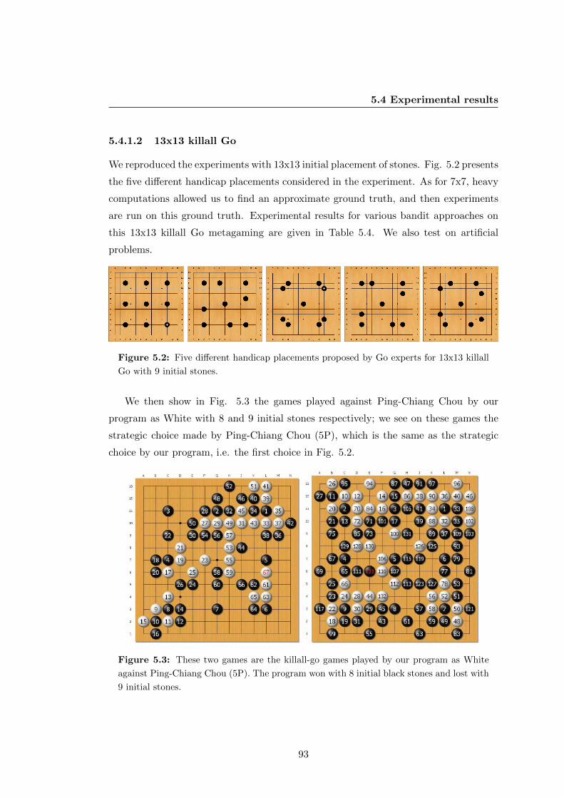
5.4 Experimental results
5.4.1.2 13x13 killall Go
We reproduced the experiments with 13x13 initial placement of stones. Fig. 5.2 presents
the five different handicap placements considered in the experiment. As for 7x7, heavy
computations allowed us to find an approximate ground truth, and then experiments
are run on this ground truth. Experimental results for various bandit approaches on
this 13x13 killall Go metagaming are given in Table 5.4. We also test on artificial
problems.
Figure 5.2: Five different handicap placements proposed by Go experts for 13x13 killall
Go with 9 initial stones.
We then show in Fig. 5.3 the games played against Ping-Chiang Chou by our
program as White with 8 and 9 initial stones respectively; we see on these games the
strategic choice made by Ping-Chiang Chou (5P), which is the same as the strategic
choice by our program, i.e. the first choice in Fig. 5.2.
Figure 5.3: These two games are the killall-go games played by our program as White
against Ping-Chiang Chou (5P). The program won with 8 initial black stones and lost with
9 initial stones.
93

5. CONTRIBUTION ON RECOMMENDATION POLICY APPLIED ONMETAGAMING
Exploration / Recommendation Average
Algorithm simple regret
(16,64,256 time steps)
Strategic choice in 13x13 killall Go
(5 possible choices)
uniform sampling, EBA 0.0201 0.0204 0.0139
UCB+MPA 0.0215 0.0192 0.0147
UCB+UCB 0.0336 0.0274 0.0213
UCB+LCB 0.0224 0.0202 0.0137
Bernstein+LCB 0.0206 0.0206 0.0146
UCB+EBA 0.0221 0.0206 0.0137
EXP3+EDP 0.0369 0.0359 0.0357
SR 0.0239 0.0225 0.0119
adapt-UCB-E, EBA 0.0235 0.0199 0.0138
Table 5.4: Experimental results of average simple regret when comparing five different
stone placements for 9 stones in 13x13 as shown in Fig. 5.2. All experiments are reproduced
1000 times.
5.4.2 Two-player case: Sparse Adversarial Bandits for Urban Rivals
Recently [51] proposed a variant of EXP3 called TEXP3. TEXP3 takes its root into
the fact that decision making algorithms in games rarely have enough time to reach
the nice asymptotic behavior guarantied by EXP3. Also, EXP3 fails to exploit that
in most games, the number of good moves is rather low compared to the number
of possible moves K. TEXP3 is an attempt to exploit these two characteristics. It
uses the outcome of EXP3 and truncates the arms that are unlikely to be part of
the solution. Alg. 11 describes the implementation. The constant c is chosen as
1T maxi(Txi)
α for some α ∈]0, 1[ (and d accordingly), as in [51], while T is the number
of iterations executed. We set α = 0.7 in our experiments, following [51]. The natural
framework of EXP3 is a two-player game. In this section we apply EXP3 and TEXP3
to Urban Rivals, a stochastic card games available for free on Internet and that fits the
framework. The game is as follow: (1) player 1 choose a combination θ1 ∈ {1, . . . ,K1};(2) simultaneously, player 2 choose a combination θ′ ∈ {1, . . . ,K ′}; (3) then the game
is resolved (ingaming). We consider a setting in which two players choose 4 cards from
a finite set of 10 cards. There exists 104 combinations, yet by removing redundant
94

5.4 Experimental results
Figure 5.4: These two games are the killall-go games played by our program as Black
against Ping-Chiang Chou (5P). The program lost both with 8 initial black stones and
with 9 initial stones.
Algorithm 11 TEXP3 (truncated EXP3), offline truncation post-EXP3.
Let x and y be the approximate Nash equilibria as proposed by EXP3 for the row
and column players respectively.
Truncate as follows
x′i = xi if xi > c, x′i = 0 otherwise;
y′i = yi if yi > d, y′i = 0 otherwise.
Renormalize: x′′ = x′/∑
i x′i; y′′ = y′/
∑i y′i.
Output x′′, y′′.
arms, we remain with 715 different possible combinations (both K1 = K2 = 715) if
we allow the same card to be used more than once. The first objective is to test
whether EXP3 (and TEXP3) is stronger than a random player for different numbers of
iterations T . We are specifically interested in situation where T is small (compared to
K1 ×K2) as it is typically the case in games. Table 5.5 (left) present the score (in %)
of EXP3 versus a random player. EXP3 significantly beats the random player when
T > 25 000. It can thus execute a strategic choice that outperforms a random player
when they have similar tactical capabilities. As T grows, the strategic choice becomes
better. Next we look into a way to make an even better choice with a smaller T .
95

5. CONTRIBUTION ON RECOMMENDATION POLICY APPLIED ONMETAGAMING
Table 5.5: EXP3 vs Random (left) and TEXP3 vs Random (right).
T Score ±1σ
10 000 0.5042 ± 0.001
25 000 0.5278 ± 0.001
50 000 0.5421 ± 0.002
100 000 0.5749 ± 0.004
T Score ±1σ
10 000 0.7206 ± 0.005
25 000 0.7238 ± 0.003
50 000 0.7477 ± 0.002
100 000 0.7871 ± 0.006
Recently TEXP3 has been proven to outperform a random player with less information
than EXP3 (experimentally in [51], theoretically in [79]). Table 5.5 (right) presents
the performance of TEXP3 against a random player under the same settings as EXP3
above. These results are in line with previous studies; however, the improvement is
much better - probably because we have here a highly sparse problem. Even with
the lowest setting (T = 10 000), TEXP3 managed a strong performance against a
random player. Again, with little information (T << K1 × K2), TEXP3 can make
strategic choices that influence the outcome of the game positively; furthermore, it
clearly outperforms EXP3.
5.5 Conclusions
We compared various algorithms for strategic choices including widely played games
(Killall Go, a classical exercise of Go schools, and Urban Rivals); we defined strategic
choices in terms of moderate exploration budget for a simple regret criterion. We
distinguished the one-player case and the two-player case; this distinction, in bandit
terms, is a distinction between stochastic and adversarial bandits.
As clearly shown by the good performance of UCB/LCB variants, SR, and EXP3
on their original frameworks (one-player and two-player cases respectively), and by the
poor performance of EXP3 in the one-player case, this distinction is relevant. Consis-
tently with theory, bandits designed for the stochastic case (typically UCB) performed
well in the one-player case and bandits designed for the adversarial case (typically
EXP3) performed well in the two-player case. The distinction between simple regret
and cumulative regret is less striking; yet, successive rejects, which was designed for
simple regret algorithms, performed very well in particular for very small budgets.
96

5.5 Conclusions
We also show the relevance of a careful recommendation algorithm; UCB is a good
exploration algorithm, but it should be accompanied by a good recommendation strat-
egy like LCB or MPA as soon as the number of options is not negligible compared to
the number of time steps; otherwise weak poorly explored arms can be recommended.
This is however less critical than in Monte-Carlo Tree Search, where bandits are applied
many times per run (once per move in a control problem or in a game).
The results in the two-player case also suggest that sparsity should be used whenever
possible in the adversarial case; the superiority of TEXP3 over EXP3 in this context is
the most clearest contrast in this work. Whereas simple regret and cumulative regret
make little difference, even in the context of small time budget, sparse or not sparse
makes a big difference, as much as distinguishing one-player case and two-player case.We
conclude below with more details for the one-player and two-player case respectively.
5.5.1 One-player case
There are two crucial components under test: exploration algorithm, and recommenda-
tion algorithm. The most important component in strategic choices is the exploration
formula. In many of our tests (with the notable exception of very small budget, very
relevant here for our setting), the best algorithm for exploration is UCB, which is
designed for the one-player case with cumulative regret; the surprising thing is that we
here work on the simple regret, which is the natural notion of regret for the framework
of strategic choices. Nonetheless, the variant of UCB termed Adapt-UCB-E, designed
for parameter free simple regret, performs correctly. Consistently with artificial tests in
[74], UCB is non-asymptotically much better than uniform exploration variants (which
are nonetheless proved asymptotically optimal within logarithmic factors both for a
fixed distribution and in a distribution free setting, in the “simple regret” setting).
The asymptotic behavior is far from being a good approximation here. Importantly for
our framework, Successive Reject, designed for simple regret, is very stable
(never very bad) and outperforms UCB variants for the smallest budgets.
Consistently with some folklore results in Monte-Carlo Tree Search, the recommen-
dation should not be made in a UCB manner; in fact, the lower confidence bound
performed very well; we also got good results with the most played arm or
the empirically best arm, as recommendation rules. We point out that many
practitioners in the Computer-Go literature (which is based on heavily tuned bandit
97

5. CONTRIBUTION ON RECOMMENDATION POLICY APPLIED ONMETAGAMING
algorithms) use combinations of EBA and MPA and LCB as recommendation arms for
optimal performance. Consistently with intuition, EBA becomes weaker with larger
numbers of arms. This is consistent with experiments in [75]. Bernstein races per-
formed moderately well; there was no effort for tuning them and maybe they might be
improved by some tuning. Adapt-UCB-E performed well as a variant of UCB dedicated
to simple regret, but not better than SR or other UCB variants.
Results include games won against a professional player, in 7x7 Killall Go and in
13x13 Killall Go; in this case, the strategic decision is the initial choice.
5.5.2 Two-player case
In the two-player case, EXP3 (dedicated to this adversarial setting) naturally performed
well.We made experiments confirming the good behavior of the algorithm, following
[51, 80, 81]. As metagaming is a good candidate for providing sparse problems, we
tested the efficiency of the truncation algorithm TEXP3 [51], with indeed much better
results here than in the original paper (this is certainly due to the fact that, in our
metagaming context, we have a much more sparse benchmark than [51]).
Results include experiments on a real game, namely Urban Rivals; the strategic
choice consists in choosing the cards, which is directly a strategic choice setting.
Further work. Importantly, we worked only on variants of bandits which have
no expert knowledge and no similarity measure on arms; we just consider the set of
strategic possibilities with no structure on it. In the one-player case, there is already
a wide literature on how to use some prior knowledge in a bandit [82, 83, 84, 85]
(progressive widening, progressive unpruning); the use of a structure on it (a distance
between arms) is not so clear and will be the object of a future work. In the case of
two bandits operating for the two strategic choices in an adversarial setting, both the
structure and the prior knowledge are to a large extent ignored in the literature. This
is our main further work.
98

5.5 Conclusions
Exploration / Average
Recommendation simple regret
Algorithm (16,64,256 time steps)
Strategic choice in 7x7 killall Go
(with symetry-breaking; 4 possible choices)
uniform sampling, EBA 0.092 0.0603 0.0244
UCB+MPA 0.079 0.0563 0.022
UCB+UCB 0.0673 0.0523 0.0304
UCB+LCB 0.0751 0.0466 0.0222
Bernstein+LCB 0.0633 0.0537 0.0226
UCB+EBA 0.0744 0.0474 0.0185
EXP3+EDP 0.0849 0.0809 0.0748
SR 0.0627 0.0448 0.021
adapt-UCB-E, EBA 0.0707 0.0483 0.0188
4 artificial options, with reward unif. in [0, 1]
uniform sampling, EBA 0.0652 0.0197 0.00394
UCB+MPA 0.0535 0.0198 0.00453
UCB+UCB 0.064 0.0386 0.00931
UCB+LCB 0.0495 0.0142 0.00626
Bernstein+LCB 0.0563 0.0191 0.00465
UCB+EBA 0.0454 0.0175 0.00401
EXP3+EDP 0.184 0.145 0.11
SR 0.0611 0.0205 0.00681
adapt-UCB-E, EBA 0.0505 0.014 0.00478
4 artificial options, (0.1, 0, 0, 0)
uniform sampling, EBA 0.0509 0.0129 0.0002
UCB+MPA 0.0519 0.0148 0.0001
UCB+UCB 0.0695 0.0277 0.0049
UCB+LCB 0.0503 0.0155 0
Bernstein+LCB 0.0483 0.0136 0.0004
UCB+EBA 0.0501 0.014 0.0001
EXP3+EDP 0.0706 0.062 0.0524
SR 0.0532 0.0409 0.012
adapt-UCB-E, EBA 0.0528 0.014 0.0001
Exploration / Average
Recommendation simple regret
Algorithm (16,64,256 time steps)
4 artificial options, (0.9, 1, 1, 1)
uniform sampling, EBA 0.0151 0.0045 0
UCB+MPA 0.0189 0.0061 0.0001
UCB+UCB 0.0179 0.0045 0.0246
UCB+LCB 0.0167 0.006 0.0001
Bernstein+LCB 0.0168 0.0048 0
UCB+EBA 0.0165 0.0048 0.0001
EXP3+EDP 0.0209 0.0211 0.0214
SR 0.0118 0.0033 0
adapt-UCB-E, EBA 0.0152 0.0057 0
4 artificial options, (0.4, 0.5, 0.5, 0.5)
uniform sampling, EBA 0.0176 0.0088 0.0019
UCB+MPA 0.0128 0.0095 0.0027
UCB+UCB 0.0157 0.0114 0.0065
UCB+LCB 0.0142 0.0078 0.0012
Bernstein+LCB 0.0167 0.0084 0.0028
UCB+EBA 0.016 0.0094 0.002
EXP3+EDP 0.0206 0.0189 0.0174
SR 0.0175 0.0105 0.0025
adapt-UCB-E, EBA 0.0153 0.0081 0.0018
4 artificial options, (0.6, 0.5, 0.5, 0.5)
uniform sampling, EBA 0.0637 0.0527 0.0277
UCB+MPA 0.0636 0.053 0.0246
UCB+UCB 0.0675 0.0561 0.0346
UCB+LCB 0.0621 0.0494 0.0244
Bernstein+LCB 0.0643 0.0498 0.0284
UCB+EBA 0.061 0.05 0.0257
EXP3+EDP 0.0715 0.0709 0.0665
SR 0.0631 0.0531 0.03
adapt-UCB-E, EBA 0.0642 0.0509 0.0247
Table 5.6: Average simple regret for various exploration/recommendation methodologies.
Performance of various strategic systems for choosing initial placement for Black in 7x7
killall-Go. The first row is the real-world case, with 4 arms; then, we consider various cases
with the same number of arms: (1) random uniform probabilities of winning for each arm;
(2) all arms have probability 0 of winning except one arm which has probability 0.1 of
winning (3) all arms have probability 1 of winning except one arm which has probability
0.9 (4) all arms have probability 0.5 except one which has probability 0.4 (5) all arms
have probability 0.5 except one which has probability 0.6. Please note that in the artificial
cases, the index of the special arm (the arm with different reward) is randomly drawn and
is indeed not necessarily the first. Each experiment is reproduced 1000 times and standard
deviations are less than 0.04.
99

5. CONTRIBUTION ON RECOMMENDATION POLICY APPLIED ONMETAGAMING
Exploration Average
/ Recommendation simple regret
Algorithm (16,64,256 time steps)
Strategic choice in 7x7 killall Go
(without symetry-breaking; 11 possible choices)
uniform sampling, EBA 0.121 0.0973 0.0488
UCB+MPA 0.127 0.0677 0.0235
UCB+UCB 0.0835 0.0826 0.0543
UCB+LCB 0.0976 0.0656 0.0213
Bernstein+LCB 0.116 0.076 0.0488
UCB+EBA 0.104 0.0657 0.0222
EXP3+EDP 0.1 �0.1 0.094
SR 0.0987 0.0557 0.0232
adapt-UCB-E, EBA 0.103 0.067 0.023
11 artificial options, with reward unif. in [0, 1]
uniform sampling, EBA 0.172 0.0614 0.017
UCB+MPA 0.219 0.0263 0.00829
UCB+UCB 0.202 0.0837 0.0366
UCB+LCB 0.165 0.0286 0.00758
Bernstein+LCB 0.185 0.0513 0.0111
UCB+EBA 0.168 0.0273 0.00708
EXP3+EDP 0.289 0.238 0.223
SR 0.123 0.0336 0.0118
adapt-UCB-E, EBA 0.154 0.0267 0.0083
11 artificial options, (0.1, 0, . . . , 0)
uniform sampling, EBA 0.0787 0.0474 0.0073
UCB+MPA 0.0787 0.0509 0.0089
UCB+UCB 0.089 0.0773 0.038
UCB+LCB 0.0776 0.048 0.0074
Bernstein+LCB 0.0764 0.0493 0.009
UCB+EBA 0.0788 0.0498 0.0094
EXP3+EDP 0.0862 0.0814 0.0765
SR 0.0788 0.0619 0.0319
adapt-UCB-E, EBA 0.0764 0.0465 0.0079
Exploration / Average
Recommendation simple regret
algorithm (16,64,256 time steps)
11 artificial options, (0.9, 1, . . . , 1)
uniform sampling, EBA 0.0069 0.0045 0.0007
UCB+MPA 0.0072 0.005 0.0005
UCB+UCB 0.0082 0.0051 0.0005
UCB+LCB 0.0065 0.0041 0.0006
Bernstein+LCB 0.0074 0.0048 0.0003
UCB+EBA 0.0072 0.005 0.0009
EXP3+EDP 0.0076 0.0086 0.0063
SR 0.0052 0.0011 0
adapt-UCB-E, EBA 0.0072 0.0041 0.0003
11 artificial options, (0.4, 0.5, . . . , 0.5)
uniform sampling, EBA 0.0055 0.0042 0.0011
UCB+MPA 0.0071 0.0032 0.0008
UCB+UCB 0.0067 0.0037 0.0032
UCB+LCB 0.0055 0.0017 0.0004
Bernstein+LCB 0.0045 0.0039 0.0018
UCB+EBA 0.0075 0.003 0.0003
EXP3+EDP 0.0074 0.0071 0.0066
SR 0.0062 0.0023 0.001
adapt-UCB-E, EBA 0.0049 0.0025 0.0009
11 artificial options, (0.6, 0.5, . . . , 0.5)
uniform sampling, EBA 0.0892 0.0824 0.0686
UCB+MPA 0.0888 0.0764 0.0563
UCB+UCB 0.087 0.0843 0.0726
UCB+LCB 0.0875 0.0766 0.0556
Bernstein+LCB 0.0869 0.0812 0.0691
UCB+EBA 0.0862 0.0783 0.0567
EXP3+EDP 0.0887 0.0869 0.0895
SR 0.0868 0.0817 0.0622
adapt-UCB-E, EBA 0.0868 0.0776 0.0569
Table 5.7: Average simple regret of various exploration/recommendations methodologies
for various real-world or artificial problems. The first row is the real-world case, in case
we do not remove the symetries; this increases the number of possible choices to 11. This
is obviously not what we should do from the point of view of the application; we just do
this in order to generate a new test case. The same artificial cases as in the 4-options case
are reproduced with 11 options. All experiments are reproduced 1000 times and standard
deviations are less than 0.004.
100

6
Algorithm discovery
6.1 Introduction
This chapter develops an idea rather pioneering. So far we focused on improving
each component of Monte Carlo search (MCS) algorithms such as the simulation, the
selection and the recommendation policy. Here, it is the combination of the components
themselves that is under study.
Indeed, MCS algorithms rely on random simulations to evaluate the quality of states
or actions in sequential decision making problems. Most of the recent progress in MCS
algorithms has been obtained by integrating smart procedures to select the simulations
to be performed. This has led to, among other things, the Upper Confidence bounds
applied to Trees algorithm (UCT, [36]) that was popularized thanks to breakthrough
results in computer Go [37]. This algorithm relies on a game tree to store simulation
statistics and uses this tree to bias the selection of future simulations. While UCT is one
way to combine random simulations with tree search techniques, many other approaches
are possible. For example, the Nested Monte Carlo (NMC) search algorithm [86], which
obtained excellent results in the last General Game Playing competition1 [87], relies on
nested levels of search and does not require storing a game tree.
How to best bias the choice of simulations is still an active topic in MCS-related
research. Both UCT and NMC are attempts to provide generic techniques that perform
well on a wide range of problems and that work with little or no prior knowledge. While
working on such generic algorithms is definitely relevant to AI, MCS algorithms are
1http://games.stanford.edu
101

6. ALGORITHM DISCOVERY
in practice widely used in a totally different scenario, in which a significant amount of
prior knowledge is available about the game or the sequential decision making problem
to be solved.
People applying MCS techniques typically spend plenty of time exploiting their
knowledge of the target problem so as to design more efficient problem-tailored variants
of MCS. Among the many ways to do this, one common practice is automatic hyper-
parameter tuning. By way of example, the parameter C > 0 of UCT is in nearly all
applications tuned through a more or less automated trial and error procedure. While
hyper-parameter tuning is a simple form of problem-driven algorithm selection, most
of the advanced algorithm selection work is done by humans, i.e., by researchers that
modify or invent new algorithms to take the specificities of their problem into account.
The comparison and development of new MCS algorithms given a target problem is
mostly a manual search process that takes much human time and is error prone. Thanks
to modern computing power, automatic discovery is becoming a credible approach for
partly automating this process. In order to investigate this research direction, we
focus on the simplest case of (fully-observable) deterministic single-player games. Our
contribution is twofold. First, we introduce a grammar over algorithms that enables
generating a rich space of MCS algorithms. It also describes several well-known MCS
algorithms, using a particularly compact and elegant description. Second, we propose
a methodology based on multi-armed bandits for identifying the best MCS algorithm
in this space, for a given distribution over training problems. We test our approach on
three different domains. The results show that it often enables discovering new variants
of MCS that significantly outperform generic algorithms such as UCT or NMC. We
further show the good robustness properties of the discovered algorithms by slightly
changing the characteristics of the problem.
This chapter is structured as follows. Section 6.2 formalizes the class of sequential
decision making problems considered in this chapter and formalizes the corresponding
MCS algorithm discovery problem. Section 6.3 describes our grammar over MCS al-
gorithms and describes several well-known MCS algorithms in terms of this grammar.
Section 6.4 formalizes the search for a good MCS algorithm as a multi-armed bandit
problem. We experimentally evaluate our approach on different domains in Section 6.5.
Finally, we discuss related work in Section 6.6 and conclude in Section 6.7.
102

6.2 Problem statement
6.2 Problem statement
We consider the class of finite-horizon fully-observable deterministic sequential decision-
making problems. A problem P is a triple (x1, f, g) where x1 ∈ X is the initial state, f
is the transition function, and g is the reward function. The dynamics of a problem is
described by
xt+1 = f(xt, ut) t = 1, 2, . . . , T, (6.1)
where for all t, the state xt is an element of the state space X and the action ut is an
element of the action space. We denote by U the whole action space and by Ux ⊂ U
the subset of actions which are available in state x ∈ X. In the context of one player
games, xt denotes the current state of the game and Uxt are the legal moves in that
state. We make no assumptions on the nature of X but assume that U is finite. We
assume that when starting from x1, the system enters a final state after T steps and
we denote by F ⊂ X the set of these final states1. Final states x ∈ F are associated to
rewards g(x) ∈ R that should be maximized.
A search algorithm A(·) is a stochastic algorithm that explores the possible se-
quences of actions to approximately maximize
A(P = (x1, f, g)) ' argmaxu1,...,uT
g(xT+1) , (6.2)
subject to xt+1 = f(xt, ut) and ut ∈ Uxt . In order to fulfill this task, the algorithm is
given a finite amount of computational time, referred to as the budget. To facilitate
reproducibility, we focus primarily in this chapter on a budget expressed as the maxi-
mum number B > 0 of sequences (u1, . . . , uT ) that can be evaluated, or, equivalently,
as the number of calls to the reward function g(·). Note, however, that it is trivial in
our approach to replace this definition by other budget measures, as illustrated in one
of our experiments in which the budget is expressed as an amount of CPU time.
We express our prior knowledge as a distribution over problems DP , from which we
can sample any number of training problems P ∼ DP . The quality of a search algorithm
1In many problems, the time at which the game enters a final state is not fixed, but depends on
the actions played so far. It should however be noted that it is possible to make these problems fit this
fixed finite time formalism by postponing artificially the end of the game until T . This can be done,
for example, by considering that when the game ends before T , a “pseudo final state” is reached from
which, whatever the actions taken, the game will reach the real final state in T .
103

6. ALGORITHM DISCOVERY
AB(·) with budget B on this distribution is denoted by JBA (DP ) and is defined as the
expected quality of solutions found on problems drawn from DP :
JBA (DP ) = EP∼DP {ExT+1∼AB(P ){g(xT+1)}} , (6.3)
where xT+1 ∼ AB(P ) denotes the final states returned by algorithm A with budget B
on problem P .
Given a class of candidate algorithms A and given the budget B, the algorithm
discovery problem amounts to selecting an algorithm A∗ ∈ A of maximal quality:
A∗ = argmaxA∈A
JBA (DP ) . (6.4)
The two main contributions of this chapter are: (i) a grammar that enables in-
ducing a rich space A of candidate MCS algorithms, and (ii) an efficient procedure to
approximately solve Eq. 6.4.
6.3 A grammar for Monte-Carlo search algorithms
All MCS algorithms share some common underlying general principles: random sim-
ulations, look-ahead search, time-receding control, and bandit-based selection. The
grammar that we introduce in this section aims at capturing these principles in a pure
and atomic way. We first give an overall view of our approach, then present in detail
the components of our grammar, and finally describe previously proposed algorithms
by using this grammar.
6.3.1 Overall view
We call search components the elements on which our grammar operates. Formally,
a search component is a stochastic algorithm that, when given a partial sequence of
actions (u1, . . . , ut−1), generates one or multiple completions (ut, . . . , uT ) and evaluates
them using the reward function g(·). The search components are denoted by S ∈ S,
where S is the space of all possible search components.
Let S be a particular search component. We define the search algorithm AS ∈ A
as the algorithm that, given the problem P , executes S repeatedly with an empty
partial sequence of actions (), until the computational budget is exhausted. The search
104

6.3 A grammar for Monte-Carlo search algorithms
algorithm AS then returns the sequence of actions (u1, . . . , uT ) that led to the highest
reward g(·).In order to generate a rich class of search components—hence a rich class of search
algorithms—in an inductive way, we rely on search-component generators. Such gener-
ators are functions Ψ : Θ→ S that define a search component S = Ψ(θ) ∈ S when given
a set of parameters θ ∈ Θ. Our grammar is composed of five search component gener-
ators that are defined in Section 6.3.2: Ψ ∈ {simulate, repeat, lookahead, step, select}.Four of these search component generators are parametrized by sub-search components.
For example, step and lookahead are functions S → S. These functions can be nested
recursively to generate more and more evolved search components. We construct the
space of search algorithms A by performing this in a systematic way, as detailed in
Section 6.4.1.
6.3.2 Search components
Table 6.1 describes our five search component generators. Note that we distinguish
between search component inputs and search component generator parameters. All
our search components have the same two inputs: the sequence of already decided
actions (u1, . . . , ut−1) and the current state xt ∈ X. The parameters differ from one
search component generator to another. For example, simulate is parametrized by a
simulation policy πsimu and repeat is parametrized by the number of repetitions N > 0
and by a sub-search component. We now give a detailed description of these search
component generators.
Simulate. The simulate generator is parametrized by a policy πsimu ∈ Πsimu which
is a stochastic mapping from states to actions: u ∼ πsimu(x). In order to generate
the completion (ut, . . . , uT ), simulate(πsimu) repeatedly samples actions uτ according
to πsimu(xτ ) and performs transitions xτ+1 = f(xτ , uτ ) until reaching a final state. A
default choice for the simulation policy is the uniformly random policy, defined as
E{πrandom(x) = u} =
{1|Ux| if u ∈ Ux
0 otherwise.(6.5)
Once the completion (ut, . . . , uT ) is fulfilled, the whole sequence (u1, . . . , uT ) is yielded.
This operation is detailed in Figure 6.1 and proceeds as follows: (i) it computes the
reward of the final state xT+1, (ii) if the reward is larger than the largest reward found
105

6. ALGORITHM DISCOVERY
Table 6.1: Search component generators
Simulate((u1, . . . , ut−1), xt)
Param: πsimu ∈ Πsimu
for τ = t to T do
uτ ∼ πsimu(xτ )
xτ+1 ← f(xτ , uτ )
end for
yield((u1, . . . , uT ))
————————
Repeat((u1, . . . , ut−1), xt)
Param: N > 0, S ∈ S
for i = 1 to N do
invoke(S, (u1, . . . , ut−1), xt)
end for
————————
LookAhead((u1, . . . , ut−1), xt)
Param: S ∈ S
for ut ∈ Uxt do
xt+1 ← f(xt, ut)
invoke(S, (u1, . . . , ut), xt+1)
end for
————————
Step((u1, . . . , ut−1), xt)
Param: S ∈ S
for τ = t to T do
invoke(S, (u1, . . . , uτ−1), xτ )
uτ ← u∗τxτ+1 ← f(xτ , uτ )
end for
————————
Select((u1, . . . , ut−1), xt)
Param: πsel ∈ Πsel, S ∈ S
for τ = t to T do . Select
uτ ∼ πsel(x)
xτ+1 ← f(xτ , uτ )
if n(xτ+1) = 0 then
break
end if
end for
tleaf ← τ
invoke(S, (u1, . . . , utleaf ), xtleaf+1) .
Sub-search
for τ = tleaf to 1 do . Backpropagate
n(xτ+1)← n(xτ+1) + 1
n(xτ , uτ )← n(xτ , uτ ) + 1
s(xτ , uτ )← s(xτ , uτ ) + r∗
end for
n(x1)← n(x1) + 1
————————
106

6.3 A grammar for Monte-Carlo search algorithms
Figure 6.1: Yield and invoke commands
Require: g : F → R, the reward function
Require: B > 0, the computational budget
Initialize global: numCalls← 0
Initialize local: r∗ ← −∞Initialize local: (u∗1, . . . , u
∗T )← ∅
procedure Yield((u1, . . . , uT ))
r = g(x)
if r > r∗ then
r∗ ← r
(u∗1, . . . , u∗T )← (u1, . . . , uT )
end if
numCalls← numCalls+ 1
if numCalls = B then
stop search
end if
end procedure
procedure Invoke(S ∈ S, (u1, . . . , ut−1) ∈ U∗, xt ∈ X)
if t ≤ T then
S((u1, . . . , ut−1), xt)
else
yield (u1, . . . , uT )
end if
end procedure
previously, it replaces the best current solution, and (iii) if the budget B is exhausted,
it stops the search.
Since algorithm AP repeats P until the budget is exhausted, the search algorithm
Asimulate(πsimu) ∈ A is the algorithm that samples B random trajectories (u1, . . . , uT ),
evaluates each of the final state rewards g(xT+1), and returns the best found final state.
This simple random search algorithm is sometimes called Iterative Sampling [88].
Note that, in the yield procedure, the variables relative to the best current solu-
tion (r∗ and (u∗1, . . . , u∗T )) are defined locally for each search component, whereas the
numCalls counter is global to the search algorithm. This means that if S is a search
107

6. ALGORITHM DISCOVERY
component composed of different nested levels of search (see the examples below), the
best current solution is kept in memory at each level of search.
Repeat. Given a positive integer N > 0 and a search component S ∈ S, repeat(N,S) is
the search component that repeats N times the search component S. For example, S =
repeat(10, simulate(πsimu)) is the search component that draws 10 random simulations
using πsimu. The corresponding search algorithm AS is again iterative sampling, since
search algorithms repeat their search component until the budget is exhausted. In
Table 6.1, we use the invoke operation each time a search component calls a sub-search
component. This operation is detailed in Figure 6.1 and ensures that no sub-search
algorithm is called when a final state is reached, i.e., when t = T + 1.
Look-ahead. For each legal move ut ∈ Uxt , lookahead(S) computes the successor state
xt+1 = f(xt, ut) and runs the sub-search component S ∈ S starting from the sequence
(u1, . . . , ut). For example, lookahead(simulate(πsimu)) is the search component that,
given the partial sequence (u1, . . . , ut−1), generates one random trajectory for each
legal next action ut ∈ Uxt . Multiple-step look-ahead search strategies naturally write
themselves with nested calls to lookahead. As an example,
lookahead(lookahead(lookahead(simulate(πsimu))))
is a search component that runs one random trajectory per legal combination of the
three next actions (ut, ut+1, ut+2).
Step. For each remaining time step τ ∈ [t, T ], step(S) runs the sub-search com-
ponent S, extracts the action uτ from (u∗1, . . . , u∗T ) (the best currently found action
sequence, see Figure 6.1), and performs transition xτ+1 = f(xτ , uτ ). The search com-
ponent generator step enables implementing time receding search mechanisms, e.g.,
step(repeat(100, simulate(πsimu))) is the search component that selects the actions
(u1, . . . , uT ) one by one, using 100 random trajectories to select each action. As a more
evolved example, step(lookahead(lookahead(repeat(10, simulation(πsimu))))) is a time re-
ceding strategy that performs 10 random simulations for each two first actions (ut, ut+1)
to decide which action ut to select.
Select. This search component generator implements most of the behaviour of a
Monte Carlo Tree Search (MCTS, [36]). It relies on a game tree, which is a non-
uniform look-ahead tree with nodes corresponding to states and edges corresponding
108

6.3 A grammar for Monte-Carlo search algorithms
to transitions. The role of this tree is twofold: it stores statistics on the outcomes of
sub-searches and it is used to bias sub-searches towards promising sequences of actions.
A search component select(πsel, S) proceeds in three steps: the selection step relies
on the statistics stored in the game tree to select a (typically small) sub-sequence of
actions (ut, . . . , utleaf ), the sub-search step invokes the sub-search component S ∈ S
starting from (u1, . . . , utleaf ), and the backpropagation step updates the statistics to
take into account the sub-search result.
We use the following notation to denote the information stored by the look-ahead
tree: n(x, u) is the number of times the action u was selected in state x, s(x, u) is the
sum of rewards that were obtained when running sub-search after having selected action
u in state x, and n(x) is the number of times state x was selected: n(x) =∑
u∈Ux n(x, u).
In order to quantify the quality of a sub-search, we rely on the reward of the best so-
lution that was tried during that sub-search: r∗ = max g(x). In the simplest case,
when the sub-search component is S = simulate(πsimu), r∗ is the reward associated
to the final state obtained by making the random simulation with policy πsimu, as
usual in MCTS. In order to select the first actions, selection relies on a selection pol-
icy πsel ∈ Πsel, which is a stochastic function that, when given all stored information
related to state x (i.e., n(x), n(x, u), and s(x, u), ∀u ∈ Ux), selects an action u ∈ Ux.
The selection policy has two contradictory goals to pursue: exploration, trying new
sequences of actions to increase knowledge, and exploitation, using current knowledge
to bias computational efforts towards promising sequences of actions. Such explo-
ration/exploitation dilemmas are usually formalized as a multi-armed bandit problem,
hence πsel is typically one of policies commonly found in the multi-armed bandit liter-
ature. The probably most well-known such policy is UCB-1 [89]:
πucb−1C (x) = argmax
u∈Ux
s(x, u)
n(x, u)+ C
√lnn(x)
n(x, u), (6.6)
where division by zero returns +∞ and where C > 0 is a hyper-parameter that enables
the control of the exploration / exploitation tradeoff.
6.3.3 Description of previously proposed algorithms
Our grammar enables generating a large class of MCS algorithms, which includes sev-
eral already proposed algorithms. We now overview these algorithms, which can be
described particularly compactly and elegantly thanks to our grammar:
109

6. ALGORITHM DISCOVERY
� The simplest Monte Carlo algorithm in our class is Iterative Sampling. This
algorithm draws random simulations until the computational time is elapsed and
returns the best solution found:
is = simulate(πsimu). (6.7)
� In general, iterative sampling is used during a certain time to decide which action
to select (or which move to play) at each step of the decision problem. The
corresponding search component is
is′ = step(repeat(N, simulate(πsimu))), (6.8)
where N is the number of simulations performed for each decision step.
� The Reflexive Monte Carlo search algorithm introduced in [90] proposes using a
Monte Carlo search of a given level to improve the search of the upper level. The
proposed algorithm can be described as follows:
rmc(N1, N2) = step(repeat(N1, step(repeat(N2, simulate(πsimu))))), (6.9)
where N1 and N2 are called the number of meta-games and the number of games,
respectively.
� The Nested Monte Carlo (NMC) search algorithm [86] is a recursively defined
algorithm generalizing the ideas of Reflexive Monte Carlo search. NMC can be
described in a very natural way by our grammar. The basic search level l = 0 of
NMC simply performs a random simulation:
nmc(0) = simulate(πrandom) . (6.10)
The level l > 0 of NMC relies on level l − 1 in the following way:
nmc(l) = step(lookahead(nmc(l − 1))) . (6.11)
� Single-player MCTS [91, 92, 93] selects actions one after the other. In order
to select one action, it relies on select combined with random simulations. The
corresponding search component is thus
mcts(πsel, πsimu, N) = step(repeat(N, select(πsel, simulate(πsimu)))) , (6.12)
110

6.4 Bandit-based algorithm discovery
where N is the number of iterations allocated to each decision step. UCT is one
of the best known variants of MCTS. It relies on the πucb−1C selection policy and
is generally used with a uniformly random simulation policy:
uct(C,N) = mcts(πucb−1C , πrandom, N) . (6.13)
� In the spirit of the work on nested Monte Carlo, the authors of [94] proposed
the Meta MCTS approach, which replaces the simulation part of an upper-level
MCTS algorithm by a whole lower-level MCTS algorithm. While they presented
this approach in the context of two-player games, we can describe its equivalent
for one-player games with our grammar:
metamcts(πsel, πsimu, N1, N2) =
step(repeat(N1, select(πsel,mcts(πsel, πsimu, N2)) (6.14)
where N1 and N2 are the budgets for the higher-level and lower-level MCTS
algorithms, respectively.
In addition to offering a framework for describing these already proposed algorithms,
our grammar enables generating a large number of new hybrid MCS variants. We give,
in the next section, a procedure to automatically identify the best such variant for a
given problem.
6.4 Bandit-based algorithm discovery
We now move to the problem of solving Eq. 6.4, i.e., of finding, for a given problem, the
best algorithm A from among a large class A of algorithms derived with the grammar
previously defined. Solving this algorithm discovery problem exactly is impossible in
the general case since the objective function involves two infinite expectations: one over
the problems P ∼ DP and another over the outcomes of the algorithm. In order to ap-
proximately solve Eq. 6.4, we adopt the formalism of multi-armed bandits and proceed
in two steps: we first construct a finite set of candidate algorithms AD,Γ ⊂ A (Section
6.4.1), and then treat each of these algorithms as an arm and use a multi-armed ban-
dit policy to select how to allocate computational time to the performance estimation
of the different algorithms (Section 6.4.2). It is worth mentioning that this two-step
111

6. ALGORITHM DISCOVERY
approach follows a general methodology for automatic discovery that we already suc-
cessfully applied to multi-armed bandit policy discovery [38, 95], reinforcement learning
policy discovery [96], and optimal control policy discovery [97].
6.4.1 Construction of the algorithm space
We measure the complexity of a search component S ∈ S using its depth, defined
as the number of nested search components constituting S, and denote this quan-
tity by depth(S). For example, depth(simulate(πsimu)) is 1, depth(uct) is 4, and
depth(nmc(3)) is 7.
Note that simulate, repeat, and select have parameters which are not search com-
ponents: the simulation policy πsimu, the number of repetitions N , and the selection
policy πsel, respectively. In order to generate a finite set of algorithms using our gram-
mar, we rely on predefined finite sets of possible values for each of these parameters.
We denote by Γ the set of these finite domains. The discrete set AD,Γ is constructed
by enumerating all possible algorithms up to depth D with constants Γ, and is pruned
using the following rules:
� Canonization of repeat: Both search components S1 = step(repeat(2, repeat(5, Ssub)))
and S2 = step(repeat(5, repeat(2, Ssub))) involve running Ssub 10 times at each
step. In order to avoid having this kind of algorithm duplicated, we collapse
nested repeat components into single repeat components. With this rule, S1 and
S2 both reduce to step(repeat(10, Ssub)).
� Removal of nested selects: A search component such as select(πsel, select(πsel, S))
is ill-defined, since the inner select will be called with a different initial state xt
each time, making it behave randomly. We therefore exclude search components
involving two directly nested selects.
� Removal of repeat-as-root: Remember that the MCS algorithm AS ∈ A runs S
repeatedly until the computational budget is exhausted. Due to this repetition,
algorithms such as Asimulate(πsimu) and Arepeat(10,simulate(πsimu)) are equivalent. To
remove these duplicates, we reject all search components whose “root” is repeat.
In the following, ν denote the cardinality of the set of candidate algorithms: AD,Γ =
{A1, . . . , Aν}. To illustrate the construction of this set, consider a simple case where
112
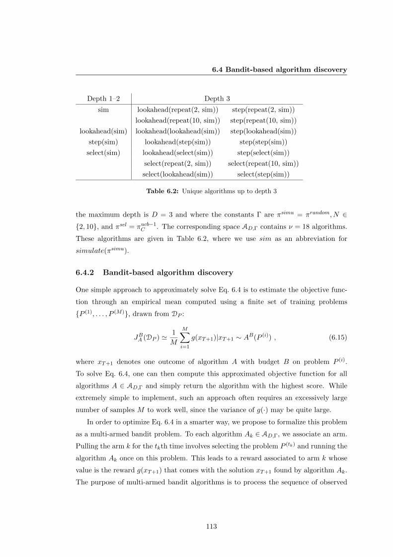
6.4 Bandit-based algorithm discovery
Depth 1–2 Depth 3
sim lookahead(repeat(2, sim)) step(repeat(2, sim))
lookahead(repeat(10, sim)) step(repeat(10, sim))
lookahead(sim) lookahead(lookahead(sim)) step(lookahead(sim))
step(sim) lookahead(step(sim)) step(step(sim))
select(sim) lookahead(select(sim)) step(select(sim))
select(repeat(2, sim)) select(repeat(10, sim))
select(lookahead(sim)) select(step(sim))
Table 6.2: Unique algorithms up to depth 3
the maximum depth is D = 3 and where the constants Γ are πsimu = πrandom, N ∈{2, 10}, and πsel = πucb−1
C . The corresponding space AD,Γ contains ν = 18 algorithms.
These algorithms are given in Table 6.2, where we use sim as an abbreviation for
simulate(πsimu).
6.4.2 Bandit-based algorithm discovery
One simple approach to approximately solve Eq. 6.4 is to estimate the objective func-
tion through an empirical mean computed using a finite set of training problems
{P (1), . . . , P (M)}, drawn from DP :
JBA (DP ) ' 1
M
M∑i=1
g(xT+1)|xT+1 ∼ AB(P (i)) , (6.15)
where xT+1 denotes one outcome of algorithm A with budget B on problem P (i).
To solve Eq. 6.4, one can then compute this approximated objective function for all
algorithms A ∈ AD,Γ and simply return the algorithm with the highest score. While
extremely simple to implement, such an approach often requires an excessively large
number of samples M to work well, since the variance of g(·) may be quite large.
In order to optimize Eq. 6.4 in a smarter way, we propose to formalize this problem
as a multi-armed bandit problem. To each algorithm Ak ∈ AD,Γ, we associate an arm.
Pulling the arm k for the tkth time involves selecting the problem P (tk) and running the
algorithm Ak once on this problem. This leads to a reward associated to arm k whose
value is the reward g(xT+1) that comes with the solution xT+1 found by algorithm Ak.
The purpose of multi-armed bandit algorithms is to process the sequence of observed
113

6. ALGORITHM DISCOVERY
rewards to select in a smart way the next algorithm to be tried, so that when the time
allocated to algorithm discovery is exhausted, one (or several) high-quality algorithm(s)
can be identified. How to select arms so as to identify the best one in a finite amount
of time is known as the pure exploration multi-armed bandit problem [98]. It has been
shown that index based policies based on upper confidence bounds such as UCB-1
were also good policies for solving pure exploration bandit problems. Our optimization
procedure works thus by repeatedly playing arms according to such a policy. In our
experiments, we perform a fixed number of such iterations. In practice this multi-armed
bandit approach can provide an answer at anytime, returning the algorithm Ak with
the currently highest empirical reward mean.
6.4.3 Discussion
Note that other approaches could be considered for solving our algorithm discovery
problem. In particular, optimization over expression spaces induced by a grammar
such as ours is often solved using Genetic Programming (GP) [99]. GP works by evolv-
ing a population of solutions, which, in our case, would be MCS algorithms. At each
iteration, the current population is evaluated, the less good solutions are removed, and
the best solutions are used to construct new candidates using mutation and cross-over
operations. Most existing GP algorithms assume that the objective function is (at least
approximately) deterministic. One major advantage of the bandit-based approach is to
natively take into account the stochasticity of the objective function and its decompos-
ability into problems. Thanks to the bandit formulation, badly performing algorithms
are quickly rejected and the computational power is more and more focused on the
most promising algorithms.
The main strengths of our bandit-based approach are the following. First, it is
simple to implement and does not require entering into the details of complex muta-
tion and cross-over operators. Second, it has only one hyper-parameter (the explo-
ration/exploitation coefficient). Finally, since it is based on exhaustive search and on
multi-armed bandit theory, formal guarantees can easily be derived to bound the regret,
i.e., the difference between the performance of the best algorithm and the performance
of the algorithm discovered [24, 98, 100].
Our approach is restricted to relatively small depths D since it relies on exhaustive
search. In our case, we believe that many interesting MCS algorithms can be described
114

6.5 Experiments
using search components with low depth. In our experiments, we used D = 5, which
already provides many original hybrid algorithms that deserve further research. Note
that GP algorithms do not suffer from such a limit, since they are able to generate
deep and complex solutions through mutation and cross-over of smaller solutions. If
the limit D = 5 was too restrictive, a major way of improvement would thus consist
in combining the idea of bandits with those of GP. In this spirit, the authors of [101]
recently proposed a hybrid approach in which the selection of the members of a new
population is posed as a multi-armed bandit problem. This enables combining the best
of the two approaches: multi-armed bandits enable taking natively into account the
stochasticity and decomposability of the objective function, while GP cross-over and
mutation operators are used to generate new candidates dynamically in a smart way.
6.5 Experiments
We now apply our automatic algorithm discovery approach to three different testbeds:
Sudoku, Symbolic Regression, and Morpion Solitaire. The aim of our experiments was
to show that our approach discovers MCS algorithms that outperform several generic
(problem independent) MCS algorithms: outperforms them on the training instances,
on new testing instances, and even on instances drawn from distributions different from
the original distribution used for the learning.
We first describe the experimental protocol in Section 6.5.1. We perform a detailed
study of the behavior of our approach applied to the Sudoku domain in Section 6.5.2.
Section 6.5.3, and 6.5.4 then give the results obtained on the other two domains. Finally,
Section 6.5.5 gives an overall discussion of our results.
6.5.1 Protocol
We now describe the experimental protocol that will be used in the remainder of this
section.
Generic algorithms. The generic algorithms are Nested Monte Carlo, Upper Confi-
dence bounds applied to Trees, Look-ahead Search, and Iterative sampling. The search
components for Nested Monte Carlo (nmc), UCT (uct), and Iterative sampling (is)
have already been defined in Section 6.3.3. The search component for Look-ahead
115
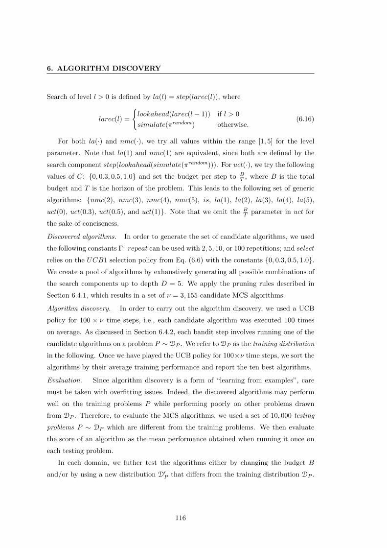
6. ALGORITHM DISCOVERY
Search of level l > 0 is defined by la(l) = step(larec(l)), where
larec(l) =
{lookahead(larec(l − 1)) if l > 0
simulate(πrandom) otherwise.(6.16)
For both la(·) and nmc(·), we try all values within the range [1, 5] for the level
parameter. Note that la(1) and nmc(1) are equivalent, since both are defined by the
search component step(lookahead(simulate(πrandom))). For uct(·), we try the following
values of C: {0, 0.3, 0.5, 1.0} and set the budget per step to BT , where B is the total
budget and T is the horizon of the problem. This leads to the following set of generic
algorithms: {nmc(2), nmc(3), nmc(4), nmc(5), is, la(1), la(2), la(3), la(4), la(5),
uct(0), uct(0.3), uct(0.5), and uct(1)}. Note that we omit the BT parameter in uct for
the sake of conciseness.
Discovered algorithms. In order to generate the set of candidate algorithms, we used
the following constants Γ: repeat can be used with 2, 5, 10, or 100 repetitions; and select
relies on the UCB1 selection policy from Eq. (6.6) with the constants {0, 0.3, 0.5, 1.0}.We create a pool of algorithms by exhaustively generating all possible combinations of
the search components up to depth D = 5. We apply the pruning rules described in
Section 6.4.1, which results in a set of ν = 3, 155 candidate MCS algorithms.
Algorithm discovery. In order to carry out the algorithm discovery, we used a UCB
policy for 100 × ν time steps, i.e., each candidate algorithm was executed 100 times
on average. As discussed in Section 6.4.2, each bandit step involves running one of the
candidate algorithms on a problem P ∼ DP . We refer to DP as the training distribution
in the following. Once we have played the UCB policy for 100×ν time steps, we sort the
algorithms by their average training performance and report the ten best algorithms.
Evaluation. Since algorithm discovery is a form of “learning from examples”, care
must be taken with overfitting issues. Indeed, the discovered algorithms may perform
well on the training problems P while performing poorly on other problems drawn
from DP . Therefore, to evaluate the MCS algorithms, we used a set of 10, 000 testing
problems P ∼ DP which are different from the training problems. We then evaluate
the score of an algorithm as the mean performance obtained when running it once on
each testing problem.
In each domain, we futher test the algorithms either by changing the budget B
and/or by using a new distribution D′P that differs from the training distribution DP .
116

6.5 Experiments
In each such experiment, we draw 10, 000 problems from D′P and run the algorithm
once on each problem.
In one domain (Morpion Solitaire), we used a particular case of our general setting,
in which there was a single training problem P , i.e., the distribution DP was degenerate
and always returned the same P . In this case, we focused our analysis on the robustness
of the discovered algorithms when tested on a new problem P ′ and/or with a new budget
B.
Presentation of the results. For each domain, we present the results in a table in which
the algorithms have been sorted according to their testing scores on DP . In each column
of these tables, we underline both the best generic algorithm and the best discovered
algorithm and show in bold all cases in which a discovered algorithm outperforms all
tested generic algorithms. We furthermore performed an unpaired t-test between each
discovered algorithm and the best generic algorithm. We display significant results
(p-value lower than 0.05) by circumscribing them with stars. As in Table 6.2, we use
sim as an abbreviation for simulate(πsimu) in this section.
6.5.2 Sudoku
Sudoku, a Japanese term meaning “singular number”, is a popular puzzle played around
the world. The Sudoku puzzle is made of a grid of G2 × G2 cells, which is structured
into blocks of size G×G. When starting the puzzle, some cells are already filled in and
the objective is to fill in the remaining cells with the numbers 1 through G2 so that
� no row contains two instances of the same number,
� no column contains two instances of the same number,
� no block contains two instances of the same number.
Sudoku is of particular interest in our case because each Sudoku grid corresponds
to a different initial state x1. Thus, a good algorithm A(·) is one that intrinsically has
the versatility to face a wide variety of Sudoku grids.
In our implementation, we maintain for each cell the list of numbers that could
be put in that cell without violating any of the three previous rules. If one of these
lists becomes empty then the grid cannot be solved and we pass to a final state (see
Footnote 2). Otherwise, we select the subset of cells whose number-list has the lowest
117

6. ALGORITHM DISCOVERY
cardinality, and define one action u ∈ Ux per possible number in each of these cells (as
in [86]). The reward associated to a final state is its proportion of filled cells, hence a
reward of 1 is associated to a perfectly filled grid.
Algorithm discovery We sample the initial states x1 by filling 33% randomly se-
lected cells as proposed in [86]. We denote by Sudoku(G) the distribution over Sudoku
problems obtained with this procedure (in the case of G2 × G2 games). Even though
Sudoku is most usually played with G = 3 [102], we carry out the algorithm discovery
with G = 4 to make the problem more difficult. Our training distribution was thus
DP = Sudoku(4) and we used a training budget of B = 1, 000 evaluations. To evaluate
the performance and robustness of the algorithms found, we tested the MCS algo-
rithms on two distributions: DP = Sudoku(4) and D′P = Sudoku(5), using a budget of
B = 1, 000.
Table 6.3 presents the results, where the scores are the average number of filled
cells, which is given by the reward times the total number of cells G4. The best
generic algorithms on Sudoku(4) are uct(0) and uct(0.3), with an average score of 198.7.
We discover three algorithms that have a better average score (198.8 and 198.9) than
uct(0), but, due to a very large variance on this problem (some Sudoku grids are far
more easy than others), we could not show this difference to be significant. Although
the discovered algorithms are not significantly better than uct(0), none of them is
significantly worst than this baseline. Furthermore, all ten discovered algorithms are
significantly better than all the other non-uct baselines. Interestingly, four out of the
ten discovered algorithms rely on the uct pattern – step(repeat(select(sim, ·), ·)) – as
shown in bold in the table.
When running the algorithms on the Sudoku(5) games, the best algorithm is still
uct(0), with an average score of 494.4. This score is slightly above the score of the best
discovered algorithm (493.7). However, all ten discovered algorithms are still signifi-
cantly better than the non-uct generic algorithms. This shows that good algorithms
with Sudoku(4) are still reasonably good for Sudoku(5).
Repeatability In order to evaluate the stability of the results produced by the bandit
algorithm, we performed five runs of algorithms discovery with different random seeds
and compared the resulting top-tens. What we observe is that our space contains a
118
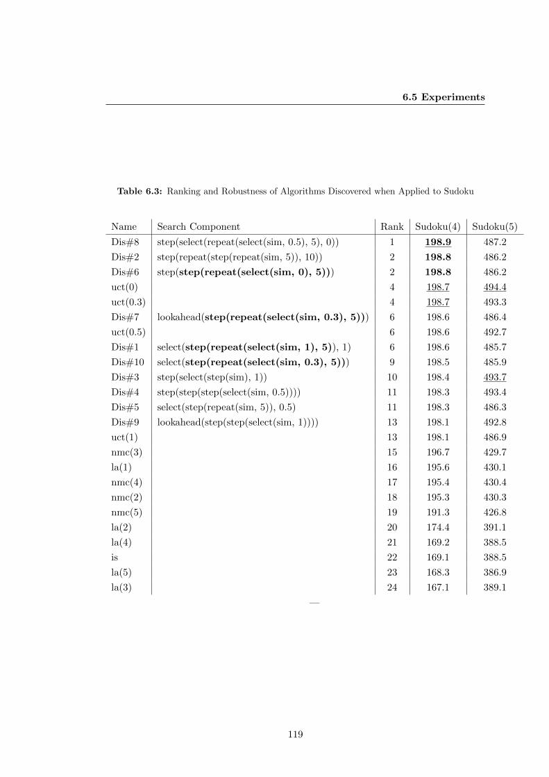
6.5 Experiments
Table 6.3: Ranking and Robustness of Algorithms Discovered when Applied to Sudoku
Name Search Component Rank Sudoku(4) Sudoku(5)
Dis#8 step(select(repeat(select(sim, 0.5), 5), 0)) 1 198.9 487.2
Dis#2 step(repeat(step(repeat(sim, 5)), 10)) 2 198.8 486.2
Dis#6 step(step(repeat(select(sim, 0), 5))) 2 198.8 486.2
uct(0) 4 198.7 494.4
uct(0.3) 4 198.7 493.3
Dis#7 lookahead(step(repeat(select(sim, 0.3), 5))) 6 198.6 486.4
uct(0.5) 6 198.6 492.7
Dis#1 select(step(repeat(select(sim, 1), 5)), 1) 6 198.6 485.7
Dis#10 select(step(repeat(select(sim, 0.3), 5))) 9 198.5 485.9
Dis#3 step(select(step(sim), 1)) 10 198.4 493.7
Dis#4 step(step(step(select(sim, 0.5)))) 11 198.3 493.4
Dis#5 select(step(repeat(sim, 5)), 0.5) 11 198.3 486.3
Dis#9 lookahead(step(step(select(sim, 1)))) 13 198.1 492.8
uct(1) 13 198.1 486.9
nmc(3) 15 196.7 429.7
la(1) 16 195.6 430.1
nmc(4) 17 195.4 430.4
nmc(2) 18 195.3 430.3
nmc(5) 19 191.3 426.8
la(2) 20 174.4 391.1
la(4) 21 169.2 388.5
is 22 169.1 388.5
la(5) 23 168.3 386.9
la(3) 24 167.1 389.1
—
119

6. ALGORITHM DISCOVERY
Table 6.4: Repeatability Analysis
Search Component Structure Occurrences in the top-ten
select(step(repeat(select(sim)))) 11
step(step(repeat(select(sim)))) 6
step(select(repeat(select(sim)))) 5
step(repeat(select(sim))) 5
select(step(repeat(sim))) 2
select(step(select(repeat(sim)))) 2
step(select(step(select(sim)))) 2
step(step(select(repeat(sim)))) 2
step(repeat(step(repeat(sim)))) 2
lookahead(step(repeat(select(sim)))) 2
step(repeat(step(repeat(sim)))) 2
select(repeat(step(repeat(sim)))) 1
select(step(repeat(sim))) 1
lookahead(step(step(select(sim)))) 1
step(step(step(select(sim)))) 1
step(step(step(repeat(sim)))) 1
step(repeat(step(select(sim)))) 1
step(repeat(step(step(sim)))) 1
step(select(step(sim))) 1
step(select(repeat(sim))) 1
—
huge number of MCS algorithms performing nearly equivalently on our distribution of
Sudoku problems. In consequence, different runs of the discovery algorithm produce
different subsets of these nearly equivalent algorithms. Since we observed that small
changes in the constants of repeat and select often have a negligible effect, we grouped
the discovered algorithms by structure, i.e. by ignoring the precise values of their
constants. Table 6.4 reports the number of occurrences of each search component
structure among the five top-tens. We observe that uct was discovered in five cases out
of fifty and that the uct pattern is part of 24 discovered algorithms.
120
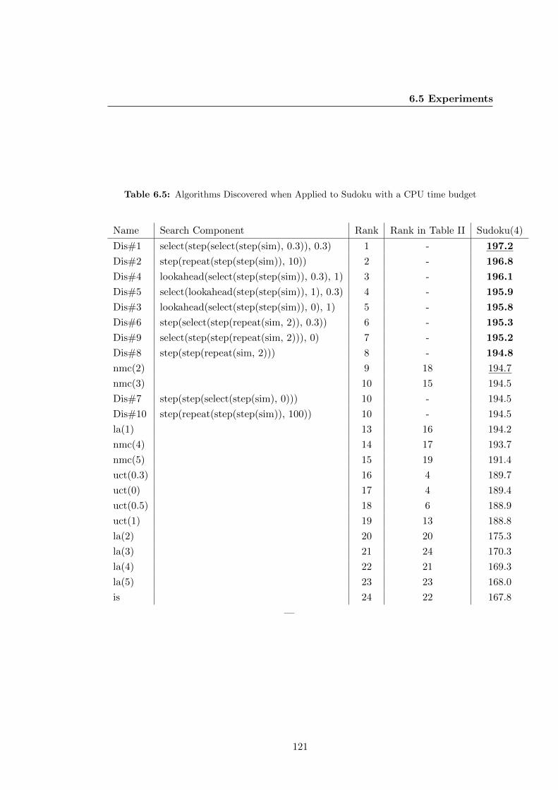
6.5 Experiments
Table 6.5: Algorithms Discovered when Applied to Sudoku with a CPU time budget
Name Search Component Rank Rank in Table II Sudoku(4)
Dis#1 select(step(select(step(sim), 0.3)), 0.3) 1 - 197.2
Dis#2 step(repeat(step(step(sim)), 10)) 2 - 196.8
Dis#4 lookahead(select(step(step(sim)), 0.3), 1) 3 - 196.1
Dis#5 select(lookahead(step(step(sim)), 1), 0.3) 4 - 195.9
Dis#3 lookahead(select(step(step(sim)), 0), 1) 5 - 195.8
Dis#6 step(select(step(repeat(sim, 2)), 0.3)) 6 - 195.3
Dis#9 select(step(step(repeat(sim, 2))), 0) 7 - 195.2
Dis#8 step(step(repeat(sim, 2))) 8 - 194.8
nmc(2) 9 18 194.7
nmc(3) 10 15 194.5
Dis#7 step(step(select(step(sim), 0))) 10 - 194.5
Dis#10 step(repeat(step(step(sim)), 100)) 10 - 194.5
la(1) 13 16 194.2
nmc(4) 14 17 193.7
nmc(5) 15 19 191.4
uct(0.3) 16 4 189.7
uct(0) 17 4 189.4
uct(0.5) 18 6 188.9
uct(1) 19 13 188.8
la(2) 20 20 175.3
la(3) 21 24 170.3
la(4) 22 21 169.3
la(5) 23 23 168.0
is 24 22 167.8
—
121

6. ALGORITHM DISCOVERY
Time-based budget Since we expressed the budget as the number of calls to the
reward function g(·), algorithms that take more time to select their actions may be
favored. To evaluate the extent of this potential bias, we performed an experiment by
setting the budget to a fixed amount of CPU time. With our C++ implementation,
on a 1.9 Ghz computer, about ≈ 350 Sudoku(4) random simulations can be performed
per second. In order to have comparable results with those obtained previously, we
thus set our budget to B = 1000350 ≈ 2.8 seconds, during both algorithm discovery and
evaluation.
Table 6.5 reports the results we obtain with a budget expressed as a fixed amount
of CPU time. For each algorithm, we indicate also its rank in Table 6.3. The new
best generic algorithm is now nmc(2) and eight out of the ten discovered have a better
average score than this generic algorithm. In general, we observe that time-based
budget favors nmc(·) algorithms and decreases the rank of uct(·) algorithms.
In order to better understand the differences between the algorithms found with
an evaluations-based budget and those found with a time-based budget, we counted
the number of occurrences of each of the search components among the ten discovered
algorithms in both cases. These counts are reported in Table 6.6. We observe that the
time-based budget favors the step search component, while reducing the use of select.
This can be explained by the fact that select is our search component that involves
the most extra-computational cost, related to the storage and the manipulation of the
game tree.
6.5.3 Real Valued Symbolic Regression
Symbolic Regression consists in searching in a large space of symbolic expressions for
the one that best fits a given regression dataset. Usually this problem is treated using
Genetic Programming approaches. In the line of [68], we here consider MCS tech-
niques as an interesting alternative to Genetic Programming. In order to apply MCS
techniques, we encode the expressions as sequences of symbols. We adopt the Reverse
Polish Notation (RPN) to avoid the use of parentheses. As an example, the sequence
[a, b,+, c, ∗] encodes the expression (a + b) ∗ c. The alphabet of symbols we used is
{x, 1,+,−, ∗, /, sin, cos, log, exp, stop}. The initial state x1 is the empty RPN sequence.
Each action u then adds one of these symbols to the sequence. When computing the
set of valid actions Ux, we reject symbols that lead to invalid RPN sequences, such
122
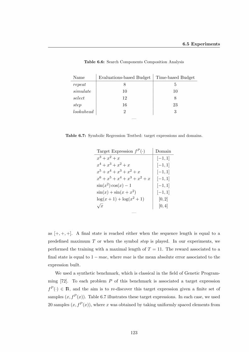
6.5 Experiments
Table 6.6: Search Components Composition Analysis
Name Evaluations-based Budget Time-based Budget
repeat 8 5
simulate 10 10
select 12 8
step 16 23
lookahead 2 3
—
Table 6.7: Symbolic Regression Testbed: target expressions and domains.
Target Expression fP (·) Domain
x3 + x2 + x [−1, 1]
x4 + x3 + x2 + x [−1, 1]
x5 + x4 + x3 + x2 + x [−1, 1]
x6 + x5 + x4 + x3 + x2 + x [−1, 1]
sin(x2) cos(x)− 1 [−1, 1]
sin(x) + sin(x+ x2) [−1, 1]
log(x+ 1) + log(x2 + 1) [0, 2]√x [0, 4]
—
as [+,+,+]. A final state is reached either when the sequence length is equal to a
predefined maximum T or when the symbol stop is played. In our experiments, we
performed the training with a maximal length of T = 11. The reward associated to a
final state is equal to 1−mae, where mae is the mean absolute error associated to the
expression built.
We used a synthetic benchmark, which is classical in the field of Genetic Program-
ming [72]. To each problem P of this benchmark is associated a target expression
fP (·) ∈ R, and the aim is to re-discover this target expression given a finite set of
samples (x, fP (x)). Table 6.7 illustrates these target expressions. In each case, we used
20 samples (x, fP (x)), where x was obtained by taking uniformly spaced elements from
123

6. ALGORITHM DISCOVERY
Table 6.8: Symbolic Regression Robustness Testbed: target expressions and domains.
Target Expression fP (·) Domain
x3 − x2 − x [−1, 1]
x4 − x3 − x2 − x [−1, 1]
x4 + sin(x) [−1, 1]
cos(x3) + sin(x+ 1) [−1, 1]√(x) + x2 [0, 4]
x6 + 1 [−1, 1]
sin(x3 + x2) [−1, 1]
log(x3 + 1) + x [0, 2]
—
the indicated domains. The training distribution DP was the uniform distribution over
the eight problems given in Table 6.7.
The training budget was B = 10, 000. We evaluate the robustness of the algorithms
found in three different ways: by changing the maximal length T from 11 to 21, by
increasing the budget B from 10,000 to 100,000 and by testing them on another distri-
bution of problems D′P . The distribution D′P is the uniform distribution over the eight
new problems given in Table 6.8.
The results are shown in Table 6.9, where we report directly the mae scores (lower
is better). The best generic algorithm is la(2) and corresponds to one of the discovered
algorithms (Dis#3). Five of the discovered algorithms significantly outperform this
baseline with scores down to 0.066. Except one of them, all discovered algorithms rely
on two nested lookahead components and generalize in some way the la(2) algorithm.
When setting the maximal length to T = 21, the best generic algorithm is again
la(2) and we have four discovered algorithms that still significantly outperform it. When
increasing the testing budget to B = 100, 000, nine discovered algorithms out of the ten
significantly outperform the best generic algorithms, la(3) and nmc(3). These results
thus show that the algorithms discovered by our approach are robust both w.r.t. the
maximal length T and the budget B.
In our last experiment with the distribution D′P , there is a single discovered al-
gorithm that significantly outperform la(2). However, all ten algorithms behave still
124

6.5 Experiments
Table 6.9: Ranking and Robustness of the Algorithms Discovered when Applied to Sym-
bolic Regression
Name Search Component Rank T = 11 T = 21 T = 11, B = 105 D′P
Dis#1 step(step(lookahead(lookahead(sim)))) 1 *0.066* *0.083* *0.036* 0.101
Dis#5 step(repeat(lookahead(lookahead(sim)), 2)) 2 *0.069* *0.085* *0.037* 0.106
Dis#2 step(lookahead(lookahead(repeat(sim, 2)))) 2 *0.069* *0.084* *0.038* 0.100
Dis#8 step(lookahead(repeat(lookahead(sim), 2))) 2 *0.069* *0.084* *0.040* 0.112
Dis#7 step(lookahead(lookahead(select(sim, 1)))) 5 *0.070* 0.087 *0.040* 0.103
Dis#6 step(lookahead(lookahead(select(sim, 0)))) 6 0.071 0.087 *0.039* 0.110
Dis#4 step(lookahead(select(lookahead(sim), 0))) 6 0.071 0.087 *0.038* 0.101
Dis#3 step(lookahead(lookahead(sim))) 6 0.071 0.086 0.056 0.100
la(2) 6 0.071 0.086 0.056 0.100
Dis#10 step(lookahead(select(lookahead(sim), 0.3))) 10 0.072 0.088 *0.040* 0.108
la(3) 11 0.073 0.090 0.053 0.101
Dis#9 step(repeat(select(lookahead(sim), 0.3), 5)) 12 0.077 0.091 *0.048* *0.099*
nmc(2) 13 0.081 0.103 0.054 0.109
nmc(3) 14 0.084 0.104 0.053 0.118
la(4) 15 0.088 0.116 0.057 0.101
nmc(4) 16 0.094 0.108 0.059 0.141
la(1) 17 0.098 0.116 0.066 0.119
la(5) 18 0.099 0.124 0.058 0.101
is 19 0.119 0.144 0.087 0.139
nmc(5) 20 0.120 0.124 0.069 0.140
uct(0) 21 0.159 0.135 0.124 0.185
uct(1) 22 0.147 0.118 0.118 0.161
uct(0.3) 23 0.156 0.112 0.135 0.177
uct(0.5) 24 0.153 0.111 0.124 0.184
—
125

6. ALGORITHM DISCOVERY
reasonably well and significantly better than the non-lookahead generic algorithms.
This result is particularly interesting since it shows that our approach was able to dis-
cover algorithms that work well for symbolic regression in general, not only for some
particular problems.
6.5.4 Morpion Solitaire
Figure 6.2: A random policy that plays the game Morpion Solitaire 5T: initial grid; after
1 move; after 10 moves; game end.
The classic game of morpion solitaire [103] is a single player, pencil and paper game,
whose world record has been improved several times over the past few years using MCS
techniques [86, 90, 104]. This game is illustrated in Figure 6.2. The initial state x1 is an
empty cross of points drawn on the intersections of the grid. Each action places a new
point at a grid intersection in such a way that it forms a new line segment connecting
consecutive points that include the new one. New lines can be drawn horizontally,
vertically, and diagonally. The game is over when no further actions can be taken. The
goal of the game is to maximize the number of lines drawn before the game ends, hence
the reward associated to final states is this number1.
There exist two variants of the game: “Disjoint” and “Touching”. “Touching”
allows parallel lines to share an endpoint, whereas “Disjoint” does not. Line segments
with different directions are always permitted to share points. The game is NP-hard
[105] and presumed to be infinite under certain configurations. In this chapter, we treat
1In practice, we normalize this reward by dividing it by 100 to make it approximately fit into the
range [0, 1]. Thanks to this normalization, we can keep using the same constants for both the UCB
policy used in the algorithm discovery and the UCB policy used in select.
126

6.5 Experiments
the 5D and 5T versions of the game, where 5 is the number of consecutive points to
form a line, D means disjoint, and T means touching.
We performed the algorithm discovery in a “single training problem” scenario: the
training distribution DP always returns the same problem P , corresponding to the 5T
version of the game. The initial state of P was the one given in the leftmost part of
Figure 6.2. The training budget was set to B = 10, 000. To evaluate the robustness of
the algorithms, we, on the one hand, evaluated them on the 5D variant of the problem
and, on the other hand, changed the evaluation budget from 10,000 to 100,000. The
former provides a partial answer to how rule-dependent these algorithms are, while the
latter gives insight into the impact of the budget on the algorithms’ ranking.
The results of our experiments on Morpion Solitaire are given in Table 6.10. Our
approach proves to be particularly successful on this domain: each of the ten discovered
algorithms significantly outperforms all tested generic algorithm. Among the generic
algorithms, la(1) gave the best results (90.63), which is 0.46 below the worst of the ten
discovered algorithms.
When moving to the 5D rules, we observe that all ten discovered algorithms still
significantly outperform the best generic algorithm. This is particularly impressive,
since it is known that the structure of good solutions strongly differs between the 5D
and 5T versions of the game [103]. The last column of Table 6.10 gives the performance
of the algorithms with budget B = 105. We observe that all ten discovered algorithms
also significantly outperform the best generic algorithm in this case. Furthermore, the
increase in the budget seems to also increase the gap between the discovered and the
generic algorithms.
6.5.5 Discussion
We have seen that on each of our three testbeds, we discovered algorithms, which are
competitive with, or even significantly better than generic ones. This demonstrates that
our approach is able to generate new MCS algorithms specifically tailored to the given
class of problems. We have performed a study of the robustness of these algorithms
by either changing the problem distribution or by varying the budget B, and found
that the algorithms discovered can outperform generic algorithms even on problems
significantly different from those used for the training.
127
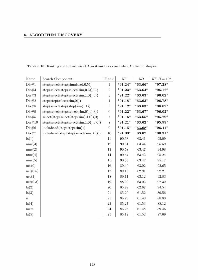
6. ALGORITHM DISCOVERY
Table 6.10: Ranking and Robustness of Algorithms Discovered when Applied to Morpion
Name Search Component Rank 5T 5D 5T,B = 105
Dis#1 step(select(step(simulate),0.5)) 1 *91.24* *63.66* *97.28*
Dis#4 step(select(step(select(sim,0.5)),0)) 2 *91.23* *63.64* *96.12*
Dis#3 step(select(step(select(sim,1.0)),0)) 3 *91.22* *63.63* *96.02*
Dis#2 step(step(select(sim,0))) 4 *91.18* *63.63* *96.78*
Dis#8 step(select(step(step(sim)),1)) 5 *91.12* *63.63* *96.67*
Dis#9 step(select(step(select(sim,0)),0.3)) 6 *91.22* *63.67* *96.02*
Dis#5 select(step(select(step(sim),1.0)),0) 7 *91.16* *63.65* *95.79*
Dis#10 step(select(step(select(sim,1.0)),0.0)) 8 *91.21* *63.62* *95.99*
Dis#6 lookahead(step(step(sim))) 9 *91.15* *63.68* *96.41*
Dis#7 lookahead(step(step(select(sim, 0)))) 10 *91.08* 63.67 *96.31*
la(1) 11 90.63 63.41 95.09
nmc(3) 12 90.61 63.44 95.59
nmc(2) 13 90.58 63.47 94.98
nmc(4) 14 90.57 63.43 95.24
nmc(5) 15 90.53 63.42 95.17
uct(0) 16 89.40 63.02 92.65
uct(0.5) 17 89.19 62.91 92.21
uct(1) 18 89.11 63.12 92.83
uct(0.3) 19 88.99 63.03 92.32
la(2) 20 85.99 62.67 94.54
la(3) 21 85.29 61.52 89.56
is 21 85.28 61.40 88.83
la(4) 23 85.27 61.53 88.12
mcts 24 85.26 61.48 89.46
la(5) 25 85.12 61.52 87.69
—
128

6.6 Related Work
The importance of each component of the grammar depends heavily on the problem.
For instance, in Symbolic Regression, all ten best algorithms discovered rely on two
nested lookahead components, whereas in Sudoku and Morpion, step and select appear
in the majority of the best algorithms discovered.
6.6 Related Work
Methods for automatically discovering MCS algorithms can be characterized through
three main components: the space of candidate algorithms, the performance criterion,
and the search method for finding the best element in the space of candidate algorithms.
Usually, researchers consider spaces of candidate algorithms that only differ in the
values of their constants. In such a context, the problem amounts to tuning the con-
stants of a generic MCS algorithm. Most of the research related to the tuning of these
constants takes as performance criterion the mean score of the algorithm over the distri-
bution of target problems. Many search algorithms have been proposed for computing
the best constants. For instance, [52] employs a grid search approach combined with
self-playing, [106] uses cross-entropy as a search method to tune an agent playing GO,
[107] presents a generic black-box optimization method based on local quadratic re-
gression, [108] uses Estimation Distribution Algorithms with Gaussian distributions,
[27] uses Thompson Sampling, and [109] uses, as in the present chapter, a multi-armed
bandit approach. The paper [110] studies the influence of the tuning of MCS algorithms
on their asymptotic consistency and shows that pathological behaviour may occur with
tuning. It also proposes a tuning method to avoid such behaviour.
Research papers that have reported empirical evaluations of several MCS algorithms
in order to find the best one are also related to this automatic discovery problem. The
space of candidate algorithms in such cases is the set of algorithms they compare, and
the search method is an exhaustive search procedure. As a few examples, [52] reports
on a comparison between algorithms that differ in their selection policy, [55] and [111]
compare improvements of the UCT algorithm (RAVE and progressive bias) with the
original one on the game of GO, and [44] evaluates different versions of a two-player
MCS algorithm on generic sparse bandit problems. [112] provides an in-depth review
of different MCS algorithms and their successes in different applications.
129

6. ALGORITHM DISCOVERY
The main feature of the approach proposed in the present chapter is that it builds
the space of candidate algorithms by using a rich grammar over the search components.
In this sense, [113, 114] are certainly the papers which are the closest to ours, since
they also use a grammar to define a search space, for, respectively, two player games
and multi-armed bandit problems. However, in both cases, this grammar only models
a selection policy and is made of classic functions such as +, −, ∗, /, log , exp , and√
. We have taken one step forward, by directly defining a grammar over the MCS
algorithms that covers very different MCS techniques. Note that the search technique
of [113] is based on genetic programming.
The decision as to what to use as the performance criterion is not as trivial as
it looks, especially for multi-player games, where opponent modelling is crucial for
improving over game-theoretically optimal play [115]. For example, the maximization
of the victory rate or loss minimization against a wide variety of opponents for a
specific game can lead to different choices of algorithms. Other examples of criteria to
discriminate between algorithms are simple regret [109] and the expected performance
over a distribution density [116].
6.7 Conclusion
In this chapter we addressed the problem of automatically identifying new Monte Carlo
search (MCS) algorithms performing well on a distribution of training problems. To
do so, we introduced a grammar over the MCS algorithms that generates a rich space
of candidate algorithms (and which describes, along the way, using a particularly com-
pact and elegant description, several well-known MCS algorithms). To efficiently search
inside this space of candidate algorithms for the one(s) having the best average perfor-
mance on the training problems, we relied on a multi-armed bandit type of optimisation
algorithm.
Our approach was tested on three different domains: Sudoku, Morpion Solitaire,
and Symbolic Regression. The results showed that the algorithms discovered this way
often significantly outperform generic algorithms such as UCT or NMC. Moreover,
we showed that they had good robustness properties, by changing the testing budget
and/or by using a testing problem distribution different from the training distribution.
130

6.7 Conclusion
This work can be extended in several ways. For the time being, we used the mean
performance over a set of training problems to discriminate between different candidate
algorithms. One direction for future work would be to adapt our general approach to use
other criteria, e.g., worst case performance measures. In its current form, our grammar
only allows using predefined simulation policies. Since the simulation policy typically
has a major impact on the performance of a MCS algorithm, it could be interesting to
extend our grammar so that it could also “generate” new simulation policies. This could
be arranged by adding a set of simulation policy generators in the spirit of our current
search component generators. Previous work has also demonstrated that the choice of
the selection policy could have a major impact on the performance of Monte Carlo tree
search algorithms. Automatically generating selection policies is thus also a direction
for future work. Of course, working with richer grammars will lead to larger candidate
algorithm spaces, which in turn, may require developing more efficient search methods
than the multi-armed bandit one used in this chapter. Finally, another important
direction for future research is to extend our approach to more general settings than
single-player games with full observability.
131

6. ALGORITHM DISCOVERY
132

7
Conclusion
This research was motivated by improving decision making under uncertainty. The
present dissertation gathers research contributions in the field of Monte Carlo Search
Algorithms. These contributions focus on the selection, the simulation and the recom-
mendation policies. Moreover, we develop a methodology to automatically generate an
MCS algorithm for a given problem.
Our contributions on the selection policy are twofold. First we categorize the selec-
tion policies into 2 main categories: Deterministic and Stochastic. We study the most
popular applied to the game of Tron and our findings in Chapter 2 are cogent with the
current literature where the deterministic policies perform better than the stochastic
ones. Second, in most of the bandit literature, it is assumed that there is no struc-
ture or similarities between arms. Thus each arm is independent from one another.
In games however, arms can be closely related. There are several good reasons for
sharing information. Chapter 3 makes use of the structure within a game. The results,
both theoretical and empirical, show a significant improvement over the state-of-the-art
selection policies.
In Chapter 4, we ponder on how to consistently generate different expressions by
changing the probability to draw each symbol. We formalize the situation into an
optimization problem and try different approaches. When the length of an expression
is relatively small (as in the simple example), it is easy to enumerate all the possible
combinations and validate our answer. However, we are interested into situations where
the length is too big to allow an enumeration (for instance a length of 25 or 30). We
133

7. CONCLUSION
show a clear improvement in the sampling process for any length. We further test the
best approach by embedding it into a MCS algorithm and it still show an improvement.
A recommendation policy is the policy to use when you make the actual decision,
which has nothing to do with the strategy of how you gather the information. The
selection policy and the recommendation policy are mutually dependent. A good rec-
ommendation policy is a policy that works well with a given selection policy. There
exists several different strategies of recommendation and Chapter 5 studies the most
common in combination with selection policies. There is a trend that seems to favor a
robust recommendation policy over a riskier one.
Chapter 6 presents a contribution where the idea is to first list the core components
upon which most MCS algorithms are built upon. From this list of core components
we automatically generate several MCS algorithms and propose a methodology based
on multi-armed bandits for identifying the best MCS algorithm(s) for a given problem.
The results show that it often enables discovering new variants of MCS that significantly
outperform generic MCS algorithms. This contribution is significant because it presents
an approach to provide a customized MCS algorithm for a given problem.
Most of the future work is presented at the end of each chapter. As a global future
work, an interesting research is to gather all the contributions presented in this thesis
together in a global algorithm. For instance, in Chapter 4 we found a way to efficiently
generate expressions. Potentially we can generate our own selection policy through
this process. If it was to be embedded into an automatic generation of algorithm as
presented in Chapter 6, then we would have an algorithm that, given a problem, can
generate its own fully customized MCS algorithm, including the selection policy. The
runtime of such an algorithm is likely to be a heavy constraint, yet the idea of no human
intervention is thrilling.
134

References
[1] Nicholas Metropolis. The beginning of the Monte
Carlo method. Los Alamos Science, 15(584):125–130,
1987. 2
[2] Jun S Liu. Monte Carlo strategies in scientific computing.
Springer, 2008. 2
[3] Marco Dorigo, Luca Maria Gambardella, Mauro Birat-
tari, Alcherio Martinoli, Riccardo Poli, and Thomas
Stutzle. Ant Colony Optimization and Swarm Intelli-
gence: 5th International Workshop, ANTS 2006, Brus-
sels, Belgium, September 4-7, 2006, Proceedings, 4150.
Springer, 2006. 2
[4] David Ruppert, Matthew P Wand, and Raymond J Car-
roll. Semiparametric regression, 12. Cambridge Uni-
versity Press, 2003. 2
[5] Petar M Djuric, Jayesh H Kotecha, Jianqui Zhang, Yufei
Huang, Tadesse Ghirmai, Monica F Bugallo, and Joaquin
Miguez. Particle filtering. Signal Processing Magazine,
IEEE, 20(5):19–38, 2003. 2
[6] John Gittins, Kevin Glazebrook, and Richard Weber.
Multi-armed bandit allocation indices. Wiley, 2011. 3
[7] Peter Auer, Nicolo Cesa-Bianchi, and Paul Fischer.
Finite-time analysis of the multiarmed bandit
problem. Machine learning, 47(2):235–256, 2002. 3,
88
[8] Michael N Katehakis and Arthur F Veinott. The
multi-armed bandit problem: decomposition and
computation. Mathematics of Operations Research,
12(2):262–268, 1987. 3
[9] Richard Weber. On the Gittins index for multi-
armed bandits. The Annals of Applied Probability,
pages 1024–1033, 1992. 3
[10] L Kocsis and Cs Szepesvari. Bandit Based Monte-
Carlo Planning. In 15th European Conference on Ma-
chine Learning (ECML), pages 282–293, 2006. 5, 90
[11] G. Chaslot, J.T. Saito, B. Bouzy, J. Uiterwijk, and H.J.
Van Den Herik. Monte Carlo Strategies for Com-
puter Go. In Proceedings of the 18th BeNeLux Confer-
ence on Artificial Intelligence, Namur, Belgium, pages
83–91, 2006. 5, 16, 22, 24
[12] R. Coulom. Efficient Selectivity and Backup Oper-
ators in Monte-Carlo Tree Search. Computers and
Games, pages 72–83, 2007. 5, 11, 25
[13] G.M.J.B. Chaslot. Monte Carlo Tree Search. PhD the-
sis, Ph. D. thesis, Department of Knowledge Engineer-
ing, Maastricht University, Maastricht, The Nether-
lands.[19, 20, 22, 31], 2010. 5, 16
[14] S. Gelly, Y. Wang, R. Munos, and O. Teytaud. Modifi-
cation of UCT with Patterns in Monte Carlo Go.
Research report, INRIA, 2006. 5, 17
[15] A.L. Samuel. Some Studies in Machine Learning
using the Game of Checkers. IBM Journal of re-
search and development, 44(1.2):206–226, 2000. 11
[16] M. Campbell, A.J. Hoane, and F. Hsu. Deep Blue. Ar-
tificial intelligence, 134(1):57–83, 2002. 11
[17] M. Muller. Computer Go. Artificial Intelligence,
134(1):145–179, 2002. 11
[18] Y. Bjornsson and H. Finnsson. CadiaPlayer: A
Simulation-Based General Game Player. IEEE
Transactions on Computational Intelligence and AI in
Games, 1(1):4–15, 2009. 11
[19] S. Samothrakis, D. Robles, and S.M. Lucas. A UCT
Agent for Tron: Initial Investigations. In Proceed-
ings of the IEEE Symposium on Computational Intelli-
gence and Games, pages 365–371, 2010. 11, 12, 15, 20,
30
[20] S.M. Lucas. Evolving a Neural Network Location
Evaluator to Play Ms. Pac-Man. In Proceedings of
the IEEE Symposium on Computational Intelligence and
Games, pages 203–210. Citeseer, 2005. 11
[21] N.G.P. Den Teuling. Monte Carlo Tree Search for
the Simultaneous Move Game Tron. Univ. Maas-
tricht, Netherlands, Tech. Rep, 2011. 12, 15
[22] M. Shafiei, N. Sturtevant, and J. Schaeffer. Compar-
ing UCT versus CFR in Simultaneous Games. In
Proceedings of the General Game Playing workshop at IJ-
CAI’09, 2009. 12, 17
[23] O. Teytaud and S. Flory. Upper Confidence Trees
with Short Term Partial Information. In Proceed-
ings of the 2011 International Conference on Applications
of Evolutionary Computation - Volume Part I, EvoAppli-
cations’11, pages 153–162, 2011. 12, 17, 22, 24
[24] P. Auer, N. Cesa-Bianchi, and P. Fischer. Finite-time
analysis of the multiarmed bandit problem. Ma-
chine learning, 47(2):235–256, 2002. 12, 20, 23, 114
[25] Francis Maes, Louis Wehenkel, and Damien Ernst. Au-
tomatic discovery of ranking formulas for play-
ing with multi-armed bandits. In 9th European
workshop on reinforcement learning (EWRL), Athens,
Greece, September 2011. 13, 21
[26] J.Y. Audibert, R. Munos, and C. Szepesvari. Tuning
bandit algorithms in stochastic environments. In
Proceedings of the Conference on Algorithmic Learning
Theory (ALT), pages 150–165, Berlin, 2007. Springer-
Verlag. 13, 21
[27] O. Chapelle and L. Li. An Empirical Evaluation of
Thompson Sampling. In Proceedings of the Confer-
ence on Advances in Neural Information Processing Sys-
tems (NIPS), 2011. 13, 23, 24, 129
135

REFERENCES
[28] L.V. Allis et al. Searching for Solutions in Games and
Artificial Intelligence. Ponsen & Looijen, 1994. 14
[29] Bruno Saverino. A Monte Carlo Tree Search for playing
Tron. Master’s thesis, Montefiore, Department of Elec-
trical Engineering and Computer Science, Universite de
Liege, 2011. 15, 26
[30] H.L. Bodlaender. Complexity of Path-Forming
Games. RUU-CS, (89-29), 1989. 15
[31] H.L. Bodlaender and AJJ Kloks. Fast Algorithms for
the Tron Game on Trees. RUU-CS, (90-11), 1990.
15
[32] T. Miltzow. Tron, a combinatorial Game on ab-
stract Graphs. Arxiv preprint arXiv:1110.3211, 2011.
15
[33] P. Funes, E. Sklar, H. Juille, and J.B. Pollack. The
Internet as a Virtual Ecology: Coevolutionary
Arms Races Between Human and Artificial Pop-
ulations. Computer Science Technical Report CS-97-
197, Brandeis University, 1997. 15
[34] Pablo Funes, Elizabeth Sklar, Hugues Juille, and Jor-
dan Pollack. Animal-Animat Coevolution: Using
the Animal Population as Fitness Function. From
Animals to Animats 5: Proceedings of the Fifth Interna-
tional Conference on Simulation of Adaptive Behavior,
5:525–533, 1998. 15
[35] A. Blair, E. Sklar, and P. Funes. Co-evolution, De-
terminism and Robustness. Simulated Evolution and
Learning, pages 389–396, 1999. 15
[36] L. Kocsis and C. Szepesvari. Bandit based Monte
Carlo planning. In Proceedings of the 17th European
Conference on Machine Learning (ECML), pages 282–
293, 2006. 16, 20, 101, 108
[37] R. Coulom. Efficient Selectivity and Backup Op-
erators in Monte-Carlo Tree Search. pages 72–83.
Springer, 2007. 16, 101
[38] Francis Maes, Louis Wehenkel, and Damien Ernst.
Learning to play K-armed bandit problems. In
International Conference on Agents and Artificial Intel-
ligence (ICAART’12), Vilamoura, Algarve, Portugal,
February 2012. 21, 50, 112
[39] G. Chaslot, J.T. Saito, B. Bouzy, J. Uiterwijk, and H.J.
Van Den Herik. Monte Carlo strategies for com-
puter go. In Proceedings of the 18th BeNeLux Confer-
ence on Artificial Intelligence, Namur, Belgium, pages
83–91, 2006. 22
[40] J.Y. Audibert and S. Bubeck. Minimax policies for
adversarial and stochastic bandits. 2009. 22, 34,
39, 40
[41] R.S. Sutton and A.G. Barto. Reinforcement Learning:
An Introduction, 1. Cambridge Univ. Press, 1998. 23
[42] B.C. May and D.S. Leslie. Simulation Studies in Op-
timistic Bayesian Sampling in Contextual-Bandit
Problems. Technical report, Technical Report 11: 02,
Statistics Group, Department of Mathematics, Univer-
sity of Bristol, 2011. 24
[43] P. Auer, N. Cesa-Bianchi, Y. Freund, and R.E. Schapire.
Gambling in a rigged casino: The adversarial
multi-armed bandit problem. In Foundations of
Computer Science, 1995. Proceedings., 36th Annual Sym-
posium on, pages 322–331. IEEE, 1995. 24, 33, 37, 88
[44] D.L. St-Pierre, Q. Louveaux, and O. Teytaud. Online
Sparse bandit for Card Game. In Proceedings of
Conference on Advances in Computer Games (ACG),
2011. 24, 34, 35, 129
[45] Cheng-Wei Chou, Ping-Chiang Chou, Chang-Shing Lee,
David Lupien Saint-Pierre, Olivier Teytaud, Mei-Hui
Wang, Li-Wen Wu, and Shi-Jim Yen. Strategic Choices:
Small Budgets and Simple Regret. In Technologies
and Applications of Artificial Intelligence (TAAI), 2012
Conference on, pages 182–187. IEEE, 2012. 33, 83
[46] D.L. St-Pierre, M.H.M. Winands, and D.A. Watt. A Se-
lective Move Generator for the game Axis and
Allies. In Computational Intelligence and Games (CIG),
2010 IEEE Symposium on, pages 162–169. Citeseer,
2010. 33
[47] Steven R Grenadier. Option exercise games: An
application to the equilibrium investment strate-
gies of firms. Review of financial studies, 15(3):691–
721, 2002. 33
[48] Trey Hedden and Jun Zhang. What do you think I
think you think?: Strategic reasoning in matrix
games. Cognition, 85(1):1–36, 2002. 33
[49] Michael D Grigoriadis and Leonid G Khachiyan. A
sublinear-time randomized approximation algo-
rithm for matrix games. Operations Research Letters,
18(2):53–58, 1995. 33, 41
[50] Richard J Lipton, Evangelos Markakis, and Aranyak
Mehta. Playing large games using simple strate-
gies. In Proceedings of the 4th ACM conference on Elec-
tronic commerce, pages 36–41. ACM, 2003. 33
[51] O. Teytaud and S. Flory. Upper Confidence Trees
with Short Term Partial Information. Applica-
tions of Evolutionary Computation; EvoGames, pages
153–162, 2011. 34, 35, 37, 38, 46, 91, 94, 96, 98
[52] P. Perrick, D.L. St-Pierre, F. Maes, and D. Ernst.
Comparison of Different Selection Strategies in
Monte Carlo Tree Search for the Game of Tron.
In Proceedings of the IEEE Conference on Computational
Intelligence and Games (CIG), Granada, Spain, 2012.
37, 129
[53] P. Auer. Using confidence bounds for
exploitation-exploration trade-offs. The Jour-
nal of Machine Learning Research, 3:397–422, 2003.
39
[54] Bruno Bouzy and Guillaume Chaslot. Monte-Carlo Go
reinforcement learning experiments. In Compu-
tational Intelligence and Games, 2006 IEEE Symposium
on, pages 187–194. IEEE, 2006. 49
[55] Sylvain Gelly and David Silver. Combining online
and offline knowledge in UCT. In Proceedings of
the 24th international conference on Machine learning,
pages 273–280. ACM, 2007. 49, 129
136

REFERENCES
[56] David Silver and Gerald Tesauro. Monte-Carlo simu-
lation balancing. In Proceedings of the 26th Annual In-
ternational Conference on Machine Learning, pages 945–
952. ACM, 2009. 49
[57] Francis Maes, Louis Wehenkel, and Damien Ernst. Au-
tomatic discovery of ranking formulas for playing
with multi-armed bandits. In 9th European workshop
on reinforcement learning (EWRL’11), Athens, Greece,
September 2011. 50
[58] Francis Maes, David Lupien St-Pierre, and Damien Ernst.
Monte Carlo Search Algorithm Discovery for
One Player Games. In To appear in IEEE Trans-
actions on Computational Intelligence and AI in Games,
arXiv 1208.4692, 2013. 50
[59] Y. Hu and S.X. Yang. A knowledge based genetic
algorithm for path planning of a mobile robot.
In Proceedings of the IEEE International Conference on
Robotics and Automation(ICRA’04), 5, pages 4350–
4355. IEEE, 2004. 50
[60] Hillol Kargupta and Kevin Buescher. The Gene Ex-
pression Messy Genetic Algorithm For Financial
Applications. In Proceedings of the IEEE International
Conference on Evolutionary Computation, pages 814–
819. IEEE Press, 1996. 50
[61] G. Jones, P. Willett, R.C. Glen, A.R. Leach, and R. Tay-
lor. Development and validation of a genetic al-
gorithm for flexible docking1. Journal of molecular
biology, 267(3):727–748, 1997. 50
[62] U. Maulik and S. Bandyopadhyay. Genetic algorithm-
based clustering technique. Pattern recognition,
33(9):1455–1465, 2000. 50
[63] S. Kikuchi, D. Tominaga, M. Arita, K. Takahashi, and
M. Tomita. Dynamic modeling of genetic networks
using genetic algorithm and S-system. Bioinfor-
matics, 19(5):643–650, 2003. 50
[64] K. Deb, A. Pratap, S. Agarwal, and T. Meyarivan. A
fast and elitist multiobjective genetic algorithm:
NSGA-II. IEEE Transactions on Evolutionary Compu-
tation, 6(2):182–197, 2002. 50
[65] J. Koza and R. Poli. Genetic programming. Search
Methodologies, pages 127–164, 2005. 50
[66] J.H. Holland. Genetic algorithms. Scientific Ameri-
can, 267(1):66–72, 1992. 50
[67] M. O’Neill and C. Ryan. Grammatical evolu-
tion. IEEE Transactions on Evolutionary Computation,
5(4):349–358, 2001. 50
[68] T. Cazenave. Nested Monte-Carlo Expression Dis-
covery. In Proceedings of the 19th European Conference
on Artificial Intelligence (ECAI’2010), pages 1057–1058.
IOS Press, 2010. 51, 70, 75, 122
[69] D.L. St-Pierre, F. Maes, D. Ernst, and Q. Louveaux. A
Learning Procedure for Sampling Semantically
Different Valid Expressions. 2013. 51, 62
[70] D.L. St-Pierre, F. Schnitzler, and Q. Louveaux. A
Clustering Approach to Enhance a Monte-Carlo
based Method for Expressions Generation. 2013.
51
[71] J. MacQueen et al. Some Methods for Classifica-
tion and Analysis of Multivariate Observations.
In Proceedings of the fifth Berkeley Symposium on Math-
ematical Statistics and Probability, 1, page 14. Califor-
nia, USA, 1967. 67
[72] N.Q. Uy, N.X. Hoai, M. ONeill, RI McKay, and E. Galvan-
Lopez. Semantically-based crossover in genetic
programming: application to real-valued sym-
bolic regression. Genetic Programming and Evolvable
Machines, 12(2):91–119, 2011. 75, 123
[73] Tristan Cazenave. Nested Monte-Carlo Search. In
Proceedings of the 21st International Joint Conference on
Artificial Intelligence (IJCAI’09), pages 456–461, 2009.
75
[74] Sebastien Bubeck, Remi Munos, and Gilles Stoltz. Pure
Exploration in Multi-armed Bandits Problems.
In ALT, pages 23–37, 2009. 88, 89, 97
[75] Amine Bourki, Matthieu Coulm, Philippe Rolet, Olivier
Teytaud, and Paul Vayssiere. Parameter Tuning by
Simple Regret Algorithms and Multiple Simulta-
neous Hypothesis Testing. In ICINCO2010, page 10,
funchal madeira, Portugal, 2010. 88, 98
[76] T.L. Lai and H. Robbins. Asymptotically efficient
adaptive allocation rules. Advances in Applied Math-
ematics, 6:4–22, 1985. 88
[77] Volodymyr Mnih, Csaba Szepesvari, and Jean-Yves Audib-
ert. Empirical Bernstein stopping. In ICML ’08:
Proceedings of the 25th international conference on Ma-
chine learning, pages 672–679, New York, NY, USA,
2008. ACM. 89
[78] Jean-Yves Audibert and Sebastien Bubeck. Best Arm
Identification in Multi-Armed Bandits. In COLT
2010 - Proceedings, page 13 p., Haifa, Israel, 2010. 89,
90
[79] David Auger, Sylvie Ruette, and Olivier Teytaud.
Sparse bandit algorithms. submitted, 2012. 96
[80] Bruno Bouzy and Marc Metivier. Multi-agent Learn-
ing Experiments on Repeated Matrix Games. In
ICML, pages 119–126, 2010. 98
[81] David Auger. Multiple Tree for Partially Observ-
able Monte-Carlo Tree Search. In EvoApplications
(1), pages 53–62, 2011. 98
[82] Remi Coulom. Computing Elo Ratings of Move Pat-
terns in the Game of Go. In Computer Games Work-
shop, Amsterdam, The Netherlands, 2007. 98
[83] Chang-Shing Lee, Mei-Hui Wang, Guillaume Chaslot,
Jean-Baptiste Hoock, Arpad Rimmel, Olivier Teytaud,
Shang-Rong Tsai, Shun-Chin Hsu, and Tzung-Pei Hong.
The Computational Intelligence of MoGo Re-
vealed in Taiwan’s Computer Go Tournaments.
IEEE Transactions on Computational Intelligence and AI
in games, 2009. 98
[84] G.M.J.B. Chaslot, M.H.M. Winands, J.W.H.M. Uiterwijk,
H.J. van den Herik, and B. Bouzy. Progressive Strate-
gies for Monte-Carlo Tree Search. In P. Wang
et al., editors, Proceedings of the 10th Joint Conference
on Information Sciences (JCIS 2007), pages 655–661.
World Scientific Publishing Co. Pte. Ltd., 2007. 98
137

REFERENCES
[85] Adrien Couetoux, Jean-Baptiste Hoock, Nataliya
Sokolovska, Olivier Teytaud, and Nicolas Bonnard.
Continuous Upper Confidence Trees. In LION’11:
Proceedings of the 5th International Conference on
Learning and Intelligent OptimizatioN, page TBA,
Italie, January 2011. 98
[86] T. Cazenave. Nested Monte Carlo Search. In
Proceedings of the 21st International Joint Conference
on Artificial Intelligence (IJCAI), pages 456–461, 2009.
101, 110, 118, 126
[87] J. Mehat and T. Cazenave. Combining UCT and
Nested Monte Carlo Search for Single-Player
General Game Playing. IEEE Transactions on Com-
putational Intelligence and AI in Games, 2(4):271–277,
2010. 101
[88] G. Tesauro and G. R. Galperin. On-line Policy Im-
provement using Monte Carlo Search. In Pro-
ceedings of the Conference on Advances in Neural Infor-
mation Processing Systems 9 (NIPS), pages 1068–1074,
1996. 107
[89] P. Auer, P. Fischer, and N. Cesa-Bianchi. Finite-time
Analysis of the Multi-armed Bandit Problem.
Machine Learning, 47:235–256, 2002. 109
[90] T. Cazenave. Reflexive Monte Carlo Search. In
Proceedings of Computer Games Workshop 2007 (CGW),
pages 165–173, Amsterdam, 2007. 110, 126
[91] G. Chaslot, S. de Jong, J-T. Saito, and J. Uiterwijk.
Monte-Carlo Tree Search in Production Manage-
ment Problems. In Proceedings of the Benelux Confer-
ence on Artificial Intelligence (BNAIC), 2006. 110
[92] Maarten P. D. Schadd, Mark H. M. Winands, H. Jaap
Van Den Herik, Guillaume M. J b. Chaslot, and Jos W.
H. M. Uiterwijk. Single-player Monte-Carlo Tree
Search. In Proceedings of Computers and Games (CG),
Lecture Notes in Computer Science, 5131, pages 1–12.
Springer, 2008. 110
[93] F. De Mesmay, A. Rimmel, Y. Voronenko, and M. Puschel.
Bandit-Based Optimization on Graphs with Ap-
plication to Library Performance Tuning. In
Proceedings of the International Conference on Machine
Learning (ICML), Montreal, Canada, 2009. 110
[94] G.M.J-B. Chaslot, J-B. Hoock, J. Perez, A. Rimmel,
O. Teytaud, and M.H.M Winands. Meta Monte Carlo
Tree Search for Automatic Opening Book Gen-
eration. In Proceedings of IJCAI Workshop on General
Intelligence in Game Playing Agents, pages 7–12, 2009.
111
[95] F. Maes, L. Wehenkel, and D. Ernst. Meta-Learning of
Exploration/Exploitation Strategies: The Multi-
Armed Bandit Case. In Proceedings of Interna-
tional Conference on Agents and Artificial Intelligence
(ICAART) - Springer Selection, arXiv:1207.5208, 2012.
112
[96] M. Castronovo, F. Maes, R. Fonteneau, and D. Ernst.
Learning exploration/exploitation strategies for
single trajectory reinforcement learning. In Pro-
ceedings of the 10th European Workshop on Reinforce-
ment Learning (EWRL), Edinburgh, Scotland, June
2012. 112
[97] Francis Maes, Raphael Fonteneau, Louis Wehenkel, and
Damien Ernst. Policy Search in a Space of Simple
Closed-form Formulas: Towards Interpretability
of Reinforcement Learning. In Proceedings of the
Conference on Discovery Science (DS), Lyon, France,
October 2012. 112
[98] S. Bubeck, R. Munos, and G. Stoltz. Pure Exploration
in Multi-armed Bandits Problems. In Proceed-
ings of the Conference on Algorithmic Learning Theory
(ALT), pages 23–37, 2009. 114
[99] J. Koza and R. Poli. Genetic Programming. In Ed-
mund K. Burke and Graham Kendall, editors, Proceedings
of the Conference on Search Methodologies (SM), pages
127–164. Springer-Verlag, Berlin, 2005. 114
[100] P-A. Coquelin and R. Munos. Bandit Algorithms
for Tree Search. In Proceedings of the Conference on
Uncertainty in Artificial Intelligence (UAI), Vancouver,
Canada, 2007. 114
[101] J-B. Hoock and O. Teytaud. Bandit-Based genetic
programming. In Proceedings of the 13th European
Conference on Genetic Programming, EuroGP, pages
268–277, Berlin, 2010. Springer-Verlag. 115
[102] Z. Geem. Harmony Search Algorithm for Solv-
ing Sudoku. In Proceedings of International Conference
on Knowledge-Based Intelligent Information and Engi-
neering Systems (KES), pages 371–378, Berlin, 2007.
Springer-Verlag. 118
[103] C. Boyer. http://www.morpionsolitaire.com. 2012.
126, 127
[104] C.D. Rosin. Nested Rollout Policy Adaptation for
Monte Carlo Tree Search. In Proc. 22nd Int. Joint
Conf. Artif. Intell., Barcelona, Spain, pages 649–654,
2011. 126
[105] E.D. Demaine, M.L. Demaine, A. Langerman, and
S. Langerman. Morpion solitaire. Theory of Com-
puting Systems, 39(3):439–453, 2006. 126
[106] I.S.G. Chaslot, M.H.M. Winands, and H.J. van den Herik.
Parameter tuning by the cross-entropy method.
In Proceedings of the European Workshop on Reinforce-
ment Learning (EWRL), 2008. 129
[107] R. Coulom. CLOP: Confident local optimization
for noisy black-box parameter tuning. In Pro-
ceedings of the 13th International Advances in Computer
Games Conference (ACG 2011), 2011. 129
[108] Francis Maes, Louis Wehenkel, and Damien Ernst. Op-
timized look-ahead tree search policies. In Pro-
ceedings of the 9th European workshop on reinforcement
learning (EWRL), Athens, Greece, September 2011. 129
[109] A. Bourki, M. Coulom, P. Rolet, O. Teytaud,
P. Vayssiere, et al. Parameter Tuning by Simple
Regret Algorithms and Multiple Simultaneous
Hypothesis Testing. In Proceedings of the Interna-
tional Conference on Informatics in Control, Automation
and Robotics (ICINCO), 2010. 129, 130
138

REFERENCES
[110] V. Berthier, H. Doghmen, and O. Teytaud. Con-
sistency modifications for automatically tuned
Monte Carlo tree search. In Proceedings of the
4th Conference on Learning and Intelligent Optimization
(LION), pages 111–124, 2010. 129
[111] G.M.J. Chaslot, M.H.M. Winands, H. Herik, J. Uiterwijk,
and B. Bouzy. Progressive strategies for Monte
Carlo tree search. In Proceedings of the 10th Joint
Conference on Information Sciences (JCIS), pages 655–
661, 2007. 129
[112] C. Browne, E. Powley, D. Whitehouse, S. Lucas, P. Cowl-
ing, P. Rohlfshagen, S. Tavener, D. Perez, S. Samoth-
rakis, and S. Colton. A Survey of Monte Carlo
Tree Search Methods. IEEE Transactions on Compu-
tational Intelligence and AI in Games, 4(1):1–43, 2012.
129
[113] T. Cazenave. Evolving Monte Carlo Tree Search
Algorithms. Technical report, 2007. 130
[114] F. Maes, L. Wehenkel, and D. Ernst. Automatic
discovery of ranking formulas for playing with
multi-armed bandits. In Proceedings of the 9th Eu-
ropean Workshop on Reinforcement Learning (EWRL
2011), 2011. 130
[115] D. Billings, A. Davidson, J. Schaeffer, and D. Szafron.
The challenge of poker. Artificial Intelligence, 134(1-
2):201–240, 2002. 130
[116] V. Nannen and A.E. Eiben. Relevance estimation and
value calibration of evolutionary algorithm pa-
rameters. In Proceedings of the 20th International Joint
Conference on Artifical Intelligence (IJCAI), pages 975–
980. Morgan Kaufmann Publishers, 2007. 130
139


