HAL Id: tel-00827159https://tel.archives-ouvertes.fr/tel-00827159

Submitted on 28 May 2013

HAL is a multi-disciplinary open accessarchive for the deposit and dissemination of sci-entific research documents, whether they are pub-lished or not. The documents may come fromteaching and research institutions in France orabroad, or from public or private research centers.

L’archive ouverte pluridisciplinaire HAL, estdestinée au dépôt et à la diffusion de documentsscientifiques de niveau recherche, publiés ou non,émanant des établissements d’enseignement et derecherche français ou étrangers, des laboratoirespublics ou privés.

Copyright

Contribution to algorithmic strategies for solvingcoupled thermo-mechanical problems by an

energy-consistent variational approachCharbel Bouery

To cite this version:Charbel Bouery. Contribution to algorithmic strategies for solving coupled thermo-mechanicalproblems by an energy-consistent variational approach. Materials and structures in mechanics[physics.class-ph]. Ecole Centrale de Nantes (ECN), 2012. English. tel-00827159

École Centrale Nantes

École Doctorale

Science Pour l’Ingénieur, Géosciences, Architecture

Année 2012 NoB.U. : ...

Thèse de Doctorat

Spécialité : Mécanique des solides, des matériaux, des structures et

des surfaces

Présentée et soutenue par:

Charbel BOUERY

Le 12 Décembre 2012à l’École Centrale Nantes

Contribution to algorithmic strategies for solving

coupled thermo-mechanical problems by an

energy-consistent variational approach

Jury

Président Pierre VILLON Professeur, Université de Technologie de Compiègne

Rapporteurs David DUREISSEIX Professeur, INSA LyonJörn MOSLER Professeur, TU Dortmund

Examinateurs Jean-Philippe PONTHOT Professeur, Université de LiègeFrancisco CHINESTA Professeur, Ecole Centrale de NantesLaurent STAINIER Professeur, Ecole centrale de Nantes

Directeur de thèse Laurent STAINIERLaboratoire Institut de Recherche en Génie Civil et Mécanique, École Centrale de Nantes

NoE.D. : ...

RésuméLes sources de couplage thermomécanique dans les matériaux viscoélastiques sont multiples : thermo-élasticité, dissipation visqueuse, évolution des caractéristiques mécaniques avec la température. Lasimulation numérique de ces couplages en calcul des structures présente encore un certain nombre dedéfis, spécialement lorsque les effets de couplage sont très marqués (couplage fort). De nombreusesapproches algorithmiques ont été proposées dans la littérature pour ce type de problème. Ces méthodesvont des approches monolithiques, traitant simultanément l’équilibre mécanique et l’équilibre thermique,aux approches étagées, traitant alternativement chacun des sous-problèmes mécanique et thermique.La difficulté est d’obtenir un bon compromis entre les aspects de précision, stabilité numérique et coûtde calcul. Récemment, une approche variationnelle des problèmes couplés a été proposée par Yang et al.(2006), qui permet d’écrire les équations d’équilibre mécanique et thermique sous la forme d’un prob-lème d’optimisation d’une fonctionnelle scalaire. Cette approche variationnelle présente notamment lesavantages de conduire à une formulation numérique à structure symétrique, et de permettre l’utilisationd’algorithmes d’optimisation. Dans ce travail on utilise l’approche variationnelle pour résoudre le prob-lème thermo-visco-elastique fortement couplé, puis on compare plusieurs schémas algorithmiques afinde trouver celui qui présente des meilleures performances

Mots-clés: Formulation variationnelle, couplage thermo-mécanique, problèmes couplés, thermo-visco-élasticité, approche monolithique.

AbstractSources of thermo-mechanical coupling in visco-elastic materials are various: viscous dissipation, de-pendence of material characteristics on temperature, ...Numerical simulation of these kinds of coupling can be challenging especially when strong couplingeffects are present. Various algorithmic approaches have been proposed in the literature for this typeof problem, and fall within two alternative strategies:

• Monolithic (or simultaneous) approaches that consists of resolving simultaneously mechanicaland thermal balance equations, where time stepping algorithm is applied to the full problem ofevolution.

• Staggered approaches in which the coupled system is partitioned and each partition is treatedby a different time stepping algorithm.

The goal is to obtain a good compromise between the following aspects: precision, stability and com-putational cost. Monolithic schemes have the reputation of being unconditionally stable, but they maylead to impossibly large systems, and do not take advantage of the different time scales involved in theproblem, and often lead to non-symmetric formulations. Staggered schemes were designed to overcomethese drawbacks, but unfortunately, they are conditionally stable (limited in time step size).Recently, a new variational formulation of coupled thermo-mechanical boundary value problems hasbeen proposed (Yang et al., 2006), allowing to write mechanical and thermal balance equations underthe form of an optimisation problem of a scalar energy-like functional. This functional is analysed in theframework of a thermo-visco-elastic strongly coupled problem, considering at first a simplified problem,and then a more general 2D and 3D case. The variational approach has many advantages, in particularthe fact that it leads to a symmetric numerical formulation has been exploited in deriving alternativeoptimization strategies. These various algorithmic schemes were tested and analysed aiming to find theone that exhibits the best computational costs.

Keywords: Variational formulation, thermo-mechanics, coupled problems, monolithic approaches, thermo-visco-elasticity

1

École Centrale Nantes

École Doctorale

Science Pour l’Ingénieur, Géosciences, Architecture

Année 2012 NoB.U. : ...

Thèse de Doctorat

Spécialité : Mécanique des solides, des matériaux, des structures et

des surfaces

Présentée et soutenue par:

Charbel BOUERY

Le 12 Décembre 2012à l’École Centrale Nantes

Contribution to algorithmic strategies for solving

coupled thermo-mechanical problems by an

energy-consistent variational approach

Jury

Président Pierre VILLON Professeur, Université de Technologie de Compiègne

Rapporteurs David DUREISSEIX Professeur, INSA LyonJörn MOSLER Professeur, TU Dortmund

Examinateurs Jean-Philippe PONTHOT Professeur, Université de LiègeFrancisco CHINESTA Professeur, Ecole Centrale de NantesLaurent STAINIER Professeur, Ecole centrale de Nantes

Directeur de thèse Laurent STAINIERLaboratoire Institut de Recherche en Génie Civil et Mécanique, École Centrale de Nantes

NoE.D. : ...

Acknowledgments

I would like to offer my sincerest gratitude to my supervisor Professor Laurent Stainierfor his guidance, support and encouragement throughout my Ph.D. study at the EcoleCentrale de Nantes. His outstanding expertise, advice and his human qualities made meenjoy working with him and learn a lot. I guess that without his good supervision, mythesis would not have finished.A special thanks to Prashant Rai, Kamran Ali Syed and Hodei Etxezarreta Olano forhaving lengthly discussions about teaching philosophies and life in general. AdditionallyI would like to thank Augusto Emmel-Selke, Shaopu Su, Laurent Gornet, Elias Safatlyand Chady Ghnatios for their time spent to answer my questions when I was stucked.I am grateful to my collegues in the Simulation & structure team for their help andfriendship. Additionally I want to thank many of the great friends that I have met inmy time at Nantes, Hodei Etxezarreta Olano, Willington Samedi, Josu Imaz Aranguren,Oscar Fornier, Tony Khalil, Modesto Mateos, Prashant Ray, Alexandre Langlais, RocioAguirre Garcia, Isabelle Farinotte, Farah Mourtada, Jane Becker, Vanessa Menut amongothers who made me feel at home, and given me an outlet outside the school.All these years, I owe a lot to the SWAPS-Nantes that provided me dancing and sportsactivities, thus allowed me to get away from the lab and keep my sanity in some ofthose very difficult days. A special thanks also to "café polyglotte" (language exchangeevents) organized by the association "Autour du Monde". Without these hobbies andmany good friends it would have been very hard to finish my Ph.D.A special thanks to Dr. Patrick Rozycki, Pascal Cosson and Jean-Yves monteau forthe opportunity they offered me as a teacher associate in solid mechanics, vibration andautomatics. These teaching reaffiremed my motivation to finish this degree and look foran academic position.The author would like to acknowledge the direct support of the Pays de la Loire regionduring the last three years.Last but not the least, I am grateful to the support of my family and my very closefriend Roger A-smith that i missed his company and these deep conversations we usedto share in those old days

2

Contents

1 Introduction to coupled systems 10

1.1 Introduction . . . . . . . . . . . . . . . . . . . . . . . . . . . . . . . . . . 101.2 Coupled systems . . . . . . . . . . . . . . . . . . . . . . . . . . . . . . . 111.3 Strong vs weak coupling . . . . . . . . . . . . . . . . . . . . . . . . . . . 11

1.3.1 Weak coupling . . . . . . . . . . . . . . . . . . . . . . . . . . . . 121.3.2 Strong coupling . . . . . . . . . . . . . . . . . . . . . . . . . . . . 12

1.4 Monolithic and staggered schemes . . . . . . . . . . . . . . . . . . . . . . 121.4.1 Monolithic scheme: . . . . . . . . . . . . . . . . . . . . . . . . . . 121.4.2 Staggered scheme . . . . . . . . . . . . . . . . . . . . . . . . . . . 13

1.5 Application . . . . . . . . . . . . . . . . . . . . . . . . . . . . . . . . . . 131.5.1 Monolitic approach . . . . . . . . . . . . . . . . . . . . . . . . . . 141.5.2 Staggered scheme . . . . . . . . . . . . . . . . . . . . . . . . . . . 141.5.3 Comments on respective advantages and merits . . . . . . . . . . 15

2 Basics of coupled thermo-mechanical problem 16

2.1 Introduction . . . . . . . . . . . . . . . . . . . . . . . . . . . . . . . . . . 172.2 Basics of continuum mechanics . . . . . . . . . . . . . . . . . . . . . . . 17

2.2.1 Small perturbations assumption . . . . . . . . . . . . . . . . . . . 182.2.2 Balance laws . . . . . . . . . . . . . . . . . . . . . . . . . . . . . 18

2.3 Basics of heat transfer . . . . . . . . . . . . . . . . . . . . . . . . . . . . 202.3.1 Fundamental modes of heat transfer . . . . . . . . . . . . . . . . . 21

2.4 Basics of thermodynamics . . . . . . . . . . . . . . . . . . . . . . . . . . 232.4.1 Thermodynamic state . . . . . . . . . . . . . . . . . . . . . . . . 232.4.2 Thermodynamic state variable . . . . . . . . . . . . . . . . . . . . 242.4.3 Entropy . . . . . . . . . . . . . . . . . . . . . . . . . . . . . . . . 242.4.4 Specific internal energy . . . . . . . . . . . . . . . . . . . . . . . . 242.4.5 First law of thermodynamics . . . . . . . . . . . . . . . . . . . . . 252.4.6 Free energy . . . . . . . . . . . . . . . . . . . . . . . . . . . . . . 262.4.7 Second law of thermodynamics . . . . . . . . . . . . . . . . . . . 272.4.8 Clausius-Duhem inequality . . . . . . . . . . . . . . . . . . . . . . 282.4.9 Developping the general thermo-mechanical heat equation . . . . 29

2.5 General thermo-mechanical heat equation . . . . . . . . . . . . . . . . . 312.5.1 Interpretation of coupled terms . . . . . . . . . . . . . . . . . . . 33

3

2.6 Applications . . . . . . . . . . . . . . . . . . . . . . . . . . . . . . . . . . 342.6.1 Linear thermo-elasticity . . . . . . . . . . . . . . . . . . . . . . . 342.6.2 Thermo-visco-elasticity . . . . . . . . . . . . . . . . . . . . . . . . 362.6.3 Thermo-plasticity . . . . . . . . . . . . . . . . . . . . . . . . . . . 38

3 Numerical simulation of classical coupled thermo-mechanical problems 41

3.1 Introduction . . . . . . . . . . . . . . . . . . . . . . . . . . . . . . . . . . 423.2 Finite element discretization of the classical non-symmetric thermo-mechanical

problem . . . . . . . . . . . . . . . . . . . . . . . . . . . . . . . . . . . . 433.3 Solving the coupled thermo-mechanical problem . . . . . . . . . . . . . . 463.4 Monolithic solution scheme . . . . . . . . . . . . . . . . . . . . . . . . . . 473.5 Staggered schemes . . . . . . . . . . . . . . . . . . . . . . . . . . . . . . 49

3.5.1 Isothermal staggered scheme . . . . . . . . . . . . . . . . . . . . . 493.5.2 Adiabatic staggered scheme . . . . . . . . . . . . . . . . . . . . . 51

3.6 Applications . . . . . . . . . . . . . . . . . . . . . . . . . . . . . . . . . . 533.6.1 Application of the FEM on a general thermal problem . . . . . . 533.6.2 Application to a thermo-elastic problem . . . . . . . . . . . . . . 56

4 Energy consistent variational approach to coupled thermo-mechanical

problems 68

4.1 Introduction . . . . . . . . . . . . . . . . . . . . . . . . . . . . . . . . . . 694.2 Variational formulation . . . . . . . . . . . . . . . . . . . . . . . . . . . . 704.3 Finite element approach for the variational formulation . . . . . . . . . . 714.4 Mixed boundary conditions . . . . . . . . . . . . . . . . . . . . . . . . . 744.5 Solution schemes . . . . . . . . . . . . . . . . . . . . . . . . . . . . . . . 74

4.5.1 Newton scheme . . . . . . . . . . . . . . . . . . . . . . . . . . . . 754.5.2 Alternated scheme . . . . . . . . . . . . . . . . . . . . . . . . . . 754.5.3 Uzawa-like algorithm . . . . . . . . . . . . . . . . . . . . . . . . . 76

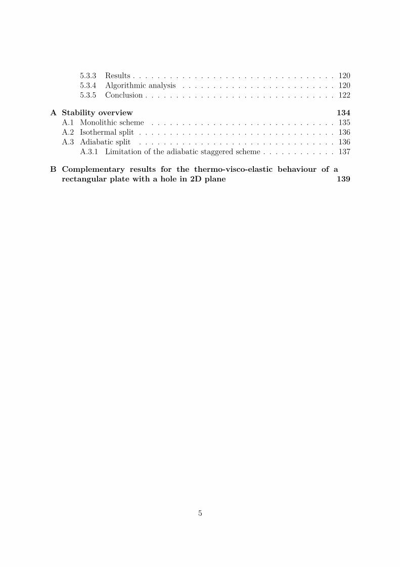
4.6 Preliminary analysis . . . . . . . . . . . . . . . . . . . . . . . . . . . . . 774.6.1 Weak coupling . . . . . . . . . . . . . . . . . . . . . . . . . . . . 784.6.2 Strong coupling . . . . . . . . . . . . . . . . . . . . . . . . . . . . 814.6.3 Conclusion . . . . . . . . . . . . . . . . . . . . . . . . . . . . . . . 83

5 Applications to coupled thermo-mechanical boundary-value problem 86

5.1 Thermo-visco-elastic behaviour of a rectangular plate with a hole in 2D . 875.1.1 Adaptive time step . . . . . . . . . . . . . . . . . . . . . . . . . . 915.1.2 Results . . . . . . . . . . . . . . . . . . . . . . . . . . . . . . . . . 925.1.3 Reference solution . . . . . . . . . . . . . . . . . . . . . . . . . . 925.1.4 Algorithmic analysis . . . . . . . . . . . . . . . . . . . . . . . . . 935.1.5 Conclusion . . . . . . . . . . . . . . . . . . . . . . . . . . . . . . . 98

5.2 Extension of the thermo-visco-elastic rectangular plate with a hole to 3D 995.3 Necking in a 3D elasto-plastic rectangular bar . . . . . . . . . . . . . . . 100

5.3.1 Elasto-plastic model . . . . . . . . . . . . . . . . . . . . . . . . . 1005.3.2 Simulation . . . . . . . . . . . . . . . . . . . . . . . . . . . . . . . 102

4

5.3.3 Results . . . . . . . . . . . . . . . . . . . . . . . . . . . . . . . . . 1205.3.4 Algorithmic analysis . . . . . . . . . . . . . . . . . . . . . . . . . 1205.3.5 Conclusion . . . . . . . . . . . . . . . . . . . . . . . . . . . . . . . 122

A Stability overview 134

A.1 Monolithic scheme . . . . . . . . . . . . . . . . . . . . . . . . . . . . . . 135A.2 Isothermal split . . . . . . . . . . . . . . . . . . . . . . . . . . . . . . . . 136A.3 Adiabatic split . . . . . . . . . . . . . . . . . . . . . . . . . . . . . . . . 136

A.3.1 Limitation of the adiabatic staggered scheme . . . . . . . . . . . . 137

B Complementary results for the thermo-visco-elastic behaviour of a

rectangular plate with a hole in 2D plane 139

5

General Introduction

With the development of science and research, the design of engineering products de-mands a more accurate description of different physics involved, since many importantengineering problems require an integrated treatment of coupled fields. In recent yearsthere has been an increasing interest in the computational modelling of coupled systems[89, 87, 112, 94, 95, 97, 100, 19, 21, 104]. Note that non-linearities and the interactionbetween its different components often results in complex systems.Coupled systems are systems whose behavior is driven by the interaction of function-ally distinct components. Multi-physics treats simulations that involve multiple physicalmodels or multiple simultaneous physical phenomena [103, 37].This field of study is so crucial, since chosen models, algorithms and implementationgrow systematically in the number of components, and often models that work correctlywith isolated components break down when coupled. Therefore it is useful to proceedin particular solution algorithms.

Sources of thermo-mechanical coupling are various in nature: thermo-elasticity, viscousdissipation, dependence of material characteristics on temperature and so on ...Numerical simulation of these kinds of coupling can be challenging, especially when astrong coupling effect is present.Various solution algorithms are found in the engineering literature of coupled problems.In the framework of this thesis we will consider concurrent approaches that can be clas-sified into two broad categories: monolithic and staggered approaches

• Monolithic (or simultaneous) approaches that consist of resolving simultaneouslymechanical and thermal balance equations, where time stepping algorithm is ap-plied to the full problem of evolution. In this case, using implicit schemes alwayslead to unconditional stability, which mean that the difference between two ini-tially close solution always remains bounded independently by the time step size[32, 43, 60, 108] etc...

• Staggered approaches where coupled system is partitioned, then each of the me-chanical and thermal problem is solved alternatively, and each partition is treatedby a different time stepping algorithm [31, 24, 108, 42, 37] etc...

6

Monolithic schemes have the advantage of being unconditionally stable, but their dis-advantage is that it might lead to impossibly large systems, same time scale involved inthe problem and this scheme is in general non-symmetric.The goal of the partitioned (or staggered) schemes is to overcome these inconveniences,but unfortunately, often at the expense of unconditional stability.In the framework of this thesis, we treat the thermo-mechanical coupled problem, viaan energy-consistent variational formulation for coupled thermo-mechanical problemsproposed by in 2006 by Yang et al [115].This variational approach has many advantages: it leads to a symmetric numerical for-mulation, possibility to derive staggered or simultaneous schemes, it is useful for adaptiveapproach (adaptive time, mesh), and allows the use of optimization algorithms in par-ticular for strongly coupled problems.

We start the first part by introducing notions about continuum thermo-mechanics, wherewe introduce basic notions of general continuum mechanics and thermodynamics andwe can write the general heat equation.Secondly, we introduce classical solving of the coupled thermo-mechanical problem, anddifferent algorithmic schemes used in the literature.Eventually, we expose the variational formulation of coupled thermo-mechanical boundary-value problem, where our work reclines.

The main objective of this framework is the validation, analysis and improvement ofmonolithic algorithmic schemes via an energy-consistent variational formulation of cou-pled thermo-mechanical problems.Since the variational formulation allows to write mechanical and thermal balance equa-tion under the form of an optimization problem of a scalar energy-like functional, differ-ent optimization algorithmic schemes will be used, the classical Newton-Raphson scheme,the alternated algorithm, and Uzawa-like algorithms.

To show the validation of the energetic formulation, and compare the efficiency of differ-ent algorithms, various applications of coupled thermo-mechanical problems have beenexposed in details, such as thermo-visco-elastic strong coupled problem from a simplifiedproblem consisting of an infinitesimal control volume to a more general 2D and 3D cou-pled thermo-elastic boundary-value problem, and then another application of a neckingin a bar with an thermo-elasto-plastic coupling.In each case the effects of heat capacity, intrinsic dissipation and the heat exchange withthe environment are included in the model.

7

Introduction générale

Les sources de couplage thermo-mécanique dans les matériaux visco-élastiques sontmultiples : thermo-élasticité, dissipation visqueuse, évolution des caractéristiques mé-caniques avec la température. La simulation numérique de ces couplages en calcul desstructures présente encore un certain nombre de défis, spécialement lorsque les effets decouplage sont très marqués (couplage fort).De nombreuses approches algorithmiques ont été proposées dans la littérature pour cetype de problème et se résument en deux stratégies alternatives:

• Approches monolithiques (ou simultanées) qui consistent de résoudre simultané-ment les équations d’équilibre mécanique et thermique. Dans ce cas, l’utilisationdes schémas implicites conduisent toujours à une stabilité inconditionelle .

• Approaches étagées où le problème thermo-mécanique est décomposé en deux sous-problèmes thermique et mécanique, et chaque partition est traité par un algorithmedifférent.

La difficulté est d’obtenir un bon compromis entre les aspects de précision, stabiliténumérique et coût de calcul.

Récemment, une approche variationnelle des problèmes couplés a été proposée par Yanget al. (2006), qui permet d’écrire les équations d’équilibre mécanique et thermique sousla forme d’un problème d’optimisation d’une fonctionnelle scalaire. Cette approche vari-ationnelle, présente notamment les avantages de conduire à une formulation numériqueà structure symétrique, et de permettre l’utilisation d’algorithmes d’optimisation.

Dans le cadre de ce travail, on s’intéresse à la validation de la formulation énergé-tique variationnelle du problème thermo-visco-mécanique couplé, ainsi que l’analyse desschémas algorithmiques monolithiques, traitant un problème allant d’un cas simplifiéconsistant en un élément de volume jusqu’au cas plus général 2D et 3D consistant enune plaque trouée en son centre et soumise à un chargement en contrainte, avec un com-portement thermo-visco-élastique de type kelvin voigt, en incluant les effects de capacitéthermique, dissipation intrinsèque et d’échange de chaleur avec l’environnement. Le cou-plage thermo-mécanique est complété en incluant une dépendance forte des coefficients

8

mécaniques par rapport à la température.Le problème thermo-visco-élastique à été testé considérant différents schémas algorith-miques dont une approche intéressante de type Uzawa qui semble réduire le temps globalde calcul. Cependant, ces résultats ont été obtenus sur un cas particulier, ce qui nousa amené à considerer un autre problème (striction d’une barre) avec un comportementelasto-plastique, où le schéma de Newton semble donner des meilleures performances.On peut conclure, d’après ce travail, que l’algorithme le plus robuste dépend du type ducouplage considéré. Cependant il reste intéressant de tester les différents schémas surd’autre type de problème (visco-plasticité etc...)

9

Chapter 1

Introduction to coupled systems

RésuméLe premier chapitre introduit des concepts généraux liés à la multi-physique et les prob-lèmes couplés.Avec l’avancement de la technologie, la simulation des systèmes mécanique demandentplus de précision. La multi-physique sera indispensable lorsqu’on a besoin de concevoirun produit qui ne peut être décrit qu’en couplant des différentes physiques. Prenant parexemple l’action du vent sur un panneau solaire, la partie de dynamique des fluides agitcomme une entrée de la partie mécanique, mais il en est de même dans le sens inverse,la partie mécanique provoque un changement de l’écoulement du fluide. Pour faire faceà ce problème, on a besoin de combiner les modèles physiques. La multi-physique reflèteplus exactement ce qui se passe dans le monde réel, qui est le but de tous les scientifiqueset les ingénieurs.

1.1 Introduction

Pace of scientific investigation and research is faster today then ever before, this accel-erated development is directly due to advancements made in understanding the laws ofnature, and in using that understanding to make better products, therefore computersimulation has emerged as an indispensable tool. In fact it is plausible to say that thefuture of technology and simulation are vitally linked. Simulation of physical systemswas one of the first applications of digital computers, with today advances and simula-tion technology and computational power one can solve just about any physics basedengineering problem on a standard PC, such as heat transfer, structural mechanics, fluiddynamics, electromagnetism, chemical reactions, acoustics and so on.The multi-physics come when we need to design a product where it can only be describedaccurately by coupling different physics, lets take for instance the wind mode on a solarpanel, the fluid dynamics part of the simulation act as input to the mechanical part, butthe same is true in reverse, the mechanics causes the change in the flow pattern. To dealwith this issue, engineers using simulation software knew to combine physical models

10

and algorithms, simulating all these physics together is required to achieve reliable sim-ulation results. Multi-physics ultimately reflects what happens in the real world moreaccurately, which is the goal for all scientists and engineers.

1.2 Coupled systems

The dictionary states eight meanings for the word "system". In multi-physics, a systemis used in the sense of a functionally related group of components forming or regardedas a collective entity [109], in other words a system is a set of interacting entities, suchas fields of continuum mechanics, evolving in time.

A coupled system is one in which physically or computationally heterogeneous me-chanical components interact dynamically. In other words a coupled system is a setof interacting sub-systems, where each sub-system is different by :

• The type of differential equation

• The type of discretization technique

• The type of physics

• The geometric domain

Sub-systems interact through interfaces, the interaction is called "one way" if there isnot feedback between subsystems for two subsystems as X and Y. The interaction iscalled "two-way" or "multiway" if there is feedback between sub-systemsWe are interested in this case, where the response has to be obtained by solving simul-taneously the coupled equations which model the system.

1.3 Strong vs weak coupling

In computational multi-physics, two types of coupling exist, strong and weak coupling.Each of those two coupling is linked directly to computational cost and performance.Consider for instance a system, where u1 and u2 are the two fields.We can write the coupled system u1(t) and u2(t) as:

du1dt

= L1(u1, u2) (1.1)du2dt

= L2(u1, u2) (1.2)

11

1.3.1 Weak coupling

A system is weakly coupled1 if sub-system 1 has significant influence on sub-system 2,while subsystem 2 has moderate (or small) influence on subsystem 1.In this case we can apply a sequential solution scheme where we can solve sub-system 1first (subsystem 1 as an input), then we solve sub-system 2.

L1(u1, u2) L1(u1) (1.3)

du1dt

L1(u1) ⇒ u1(t) (1.4)du2dt

= L2(u2, u1(t)) (1.5)

1.3.2 Strong coupling

A system is called strongly coupled2, if both sub-system 1 and sub-system 2 have influ-ences on each others.In this case we can apply different kind of schemes to solve the problem :

• Concurrent solution scheme such monolithic schemes where we solve simultane-ously all equations in one algorithm.

• Staggered schemes where the coupled problem is split and each physic is treatedby different strategy.

1.4 Monolithic and staggered schemes

1.4.1 Monolithic scheme:

Consider the interaction between two scalar fields u1 and u2, where each field has onlyone state variable u1(t) and u2(t).The monolithic scheme consists of resolving simultaneously the fields equations u(t) (inu1 and u2) with one algorithm (whether implicit or explicit), where u(t) is defined as:

1Examples of weakly coupled systems : aero-accoustics2examples of strongly coupled systems : thermo-mechanics, thermo-visco-elasticity, aero-elasticity

and so on

12

u(t) = u1(t), u2(t)T (1.6)u(0) = u0 (1.7)

dudt

= L(u) (1.8)

Therefore we obtain a complex system with a very large size, but have the benefit tobe unconditional stable for implicit algorithms, meaning that we can go for larger timesteps without affecting the stability of the system.On the other hand, explicit algorithms lead to conditional stability, which means thatthe stability of the system is influenced by the size of time step, the time step shall beless than a critical time step ∆t < ∆tcrit.If we denote ∆tcrit1 the critical time step for the stability of the sub-system 1, and ∆tcrit2

the critical time step for the stability of the sub-system 2, min(∆tcrit1 , ∆tcrit2) may be max(∆tcrit1 , ∆tcrit2)The system obtained is very large, and the tangent matrix has the following form:

δL1δu1

δL1δu2

δL2δu1

δL2δu2

(1.9)

The system obtained is generally non-symmetric due to the coupled terms of δL1δu2

andδL2δu1

, and this lead to big computational cost generated by the inversion of the tangentmatrix, especially when the coupling is strong, where the sub-diagonal matrices shouldbe taken into account. In fact, when coupling is weak, these matrices can be neglected.Strong coupling may influence convergence, but not inversion time with direct solvers.

1.4.2 Staggered scheme

The goal of a staggered scheme is to split the coupled problem into a set of sub-problems,therefore the staggered scheme (also called partitioned (without a fixed point)) solvesdifferent physic separately L(u) = L2 L1(u). The system becomes simpler due tothe reduction of degrees of freedom of each sub-system. Some of the advantages is thatwe can use the best algorithm of resolution for each sub-system, the best discretizationfor each sub-system and may use the best time increments for each sub-system (whichis not so obvious in practice). One of the disadvantages is that a staggered scheme isnot always stable [101, 102].

1.5 Application

Consider strong coupling between two scalar fields X and Y. Each field has one statevariable identified as x(t) and y(t), respectively, which are assumed to be governed by

13

the first-order differential equation:

x + ax + cy = f(t) (1.10)y + by + dx = g(t) (1.11)

where f(t) and g(t) are the applied forces.Equation 1.10 can be written in the following form:

L1(x, y) = f(t) − ax − cy (1.12)L2(x, y) = g(t) − dx − by (1.13)

or more generally Li(x, y) = Ai(x, y) + fi(t).The initial conditions are given by:

x(0) = x0 x(0) = x0 (1.14)y(0) = y0 y(0) = y0 (1.15)

1.5.1 Monolitic approach

Let’s treat the system by Backward Euler integration in each component:

xn+1 = xn + ∆txn+1 (1.16)yn+1 = yn + ∆tyn+1 (1.17)

xn+1 = xn + ∆t (f(tn+1) − axn+1 − cyn+1) (1.18)yn+1 = yn + ∆t (g(tn+1) − byn+1 − dxn+1) (1.19)

where xn = x(tn), etc. At each time step n = 0, 1, 2, ... we get:

xn+1yn+1

=

1 + a∆t c∆t

d∆t 1 + b∆t

−1 xn + ∆tfn+1yn + ∆tgn+1

(1.20)

in which [x0, y0] are provided by the initial conditions. In the monolithic or simultaneoussolution approach, the system (1.20) is solved at each time step till the final time tf .

1.5.2 Staggered scheme

The system treated above can be written as:

1 + a∆t c∆t

d∆t 1 + b∆t

xn+1yn+1

=

xn + ∆tfn+1yn + ∆tgn+1

(1.21)

14

A simple partitioned solution procedure is obtained by treating the system (1.21) withthe following staggered partition with prediction on y:

1 + a∆t 0

d∆t 1 + b∆t

xn+1yn+1

=

xn + ∆tfn+1 − c∆typ

n+1yn + ∆tgn+1

(1.22)

1. Predictor : yp

n+1 = yn + ∆tyn

2. Solve x (or Advance x) : xn+1 = 11+a∆t

(xn + ∆tfn+1 − cyp

n+1)

3. Transfer (or Substitute) : xn+1 = xn+1

4. Solve y (or Advance y) : yn+1 = 11+b∆t

(yn + ∆tgn+1 − d∆txn+1)where y

p

n+1 is the predictor. Two common choices for the predictor are yp

n+1 = yn (calledthe last solution predictor) and y

p

n+1 = yn + ∆tyn

1.5.3 Comments on respective advantages and merits

Since Backward Euler integration conserves the stability of the system, the features ofeach schemes will be commented as follows:

A scheme is called stable if the eigenvalues of the amplification matrix is < 1.

For the monolithic scheme the amplification matrix is given by

1 + a∆t c∆t

d∆t 1 + b∆t

−1

(1.23)

For the staggered scheme, we can write system (1.22) in a alternative manner, by con-sidering the predictor y

p

n+1 = yn:

1 + a∆t 0d∆t 1 + b∆t

xn+1yn+1

=

1 −c∆t

0 1

xn

yn

+

∆tfn+1∆tgn+1

(1.24)

In this case the amplification matrix is given by:

1 + a∆t 0d∆t 1 + b∆t

−1 1 −c∆t

0 1

(1.25)

If we select certain values for a, b, c and d where a > 0, b > 0 and a × b − c × d > 0, wecan see clearly that the eigenvalues of the amplification matrix (eq. 1.23) are < 1, whilethe eigenvalues of the amplification matrix (eq. 1.25) may be > 1, then we can deducethat the monolithic schemes are unconditionally stable, whereas the staggered schemesare conditionally stable.

15

Chapter 2

Basics of coupled

thermo-mechanical problem

RésuméDans ce chapitre on rappelle les concepts de base, et la formulation des équations réagis-sant le comportement d’un milieu continu, ainsi que les principes fondamentaux de lathermodynamique et du transfert de chaleur. Le formalisme développé peut prendre encompte la production de grandes déformations ainsi que les couplages pouvant apparaîtreentre les champs mécanique et thermique.

L’approche adoptée est basé sur l’hypothèse d’état local thermodynamique à l’équilibre,d’où les fonctions thermodynamique sont déterminées à partir des variables d’état, qui nedépendent que de ces derniers (indépendant de leur gradient et leur dérivées temporelles).Les variables d’état sont de trois types, décrivant l’état de déformation du corps, sa tem-pérature et sa structure interne représentée par des variables d’état interne. Le choix deces variables d’état , qui doit être bien adéquat, est une des difficultés d’utilisation de laformulation thermodynamique

Afin de développer l’équation de chaleur, qui met en evidence les termes de couplagethermo-mécanique, il convient de rappeler les fonctions thermodynamiques (comme l’énergielibre) qui sont des fonctions des variables d’état, ou bien de leur grandeur thermody-namiquement conjuguée.

A la fin de ce chapitre, l’équation de chaleur la plus générale est développée, afin demettre en évidence l’évolution de la variable température, qui se traduit par le principede conservation de l’énergie. L’équation de la chaleur est une réécriture du premierprincipe en utilisant les lois d’état et les lois complémentaire exposées dans le chapitre.Elle permet de mettre en évidence les couplages entre les effets mécaniques et thermiqueet de préciser les grandeurs énergétiques qui se transforment en chaleur lors d’un pro-cessus thermo-mécanique.

16

2.1 Introduction

In this chapter we recall the basic concepts in continuum mechanics and the fundamentalprinciples of thermodynamics and heat transfer. The theories that we examine here areall based on the assumption of local thermodynamic state in equilibrium, this meansthat the thermodynamic functions are determined through a finite set of variables, calledstate variables. These functions depending only on these variables will be independentof their gradients (local state) and their time derivatives (system in equilibrium). Inthese theories, the state variables are almost always describing three types: the state ofdeformation of the body, its temperature and internal structure [47, 83, 67, 48, 56, 98].

2.2 Basics of continuum mechanics

Continuum mechanics is a branch of mechanics that deals with the analysis of the kine-matics and the mechanical behavior of materials modelled as a continuous mass ratherthan as discrete particles. The French mathematician Augustin Louis Cauchy was thefirst to formulate such models in the 19th century, but research in the area continuestoday.On a macroscopic scale, materials have cracks and discontinuities. However, certainphysical phenomena can be modelled assuming the materials exist as a continuum, mean-ing the matter in the body is continuously distributed and fills the entire region of spaceit occupies. A continuum is a body that can be continually sub-divided into infinitesimalelements with properties being those of the bulk material.To develop an appropriate formalism, we will need to refer to two different configura-tions of a continuous body. Let B0 denotes the reference configuration that representsthe configuration at time t = t0, occupying a volume V0 defined by a boundary A0,and by Bt the current configuration at time t, occupying a volume Vt and a boundaryAt. The positions of material particles belonging to the reference configuration B0 aredenoted by X, and those belonging to the current configuration Bt, are denoted by x.Each material point will move and have its own trajectory path. Hence, the trajectoryis defined by the evolution of the material point x as follow:

x = φ(X, t) (2.1)

The gradient of the deformation relative to the motion between the reference and thecurrent configuration is defined as follow:

F = ∂φ(X, t)∂X

= ∂x(X, t)∂X

(2.2)

where F is a second order tensor.In general F is a non symmetric tensor. The measurement of deformation is dependenton the configuration (the actual configuration B0 or the current configuration Bt. Inour work, the chosen configuration is the reference configuration (B0). In this case, the

17

deformation is measured through the Green-Lagrange deformation tensor , defined by:

E = 12 (C − I) = 1

2F

TF − I

(2.3)

where the index T is the transpose of the tensor F, C = FTF is called right Cauchy-

Green stretch tensor, it is symmetric, and I is the identity tensor.

The gradient of the transformation can be written in function of the gradient of dis-placement:

F = ∂x

∂X= ∂(X + u)

∂X= I + ∂u

∂X(2.4)

Where u is the displacement vector.We can write then the Green-Lagrange tensor as follow:

E = 12(C − I) (2.5)

= 12(FT

F − I) (2.6)

= = 12

( ∂u

∂X) + ( ∂u

∂X)T + ( ∂u

∂X)T · ( ∂u

∂X)

(2.7)

2.2.1 Small perturbations assumption

Small perturbations assumption states that displacements (and rotations) between thereference and actual configuration are very small, as well as the gradient of the displace-ment.

Under these conditions (small perturbations), the current and the reference config-urations are very close to each others, then we can substitute the variable x by X, ∀x ∈ Ω, therefore we can neglect the quadratic term in equation (2.7):

E ≈ 12

∂u

∂X+ ( ∂u

∂X)T

= (2.8)

In this case, the deformation tensor of the current configuration, called Euler-Almansitensor, gives the same expression as (2.8).

2.2.2 Balance laws

Let f(x, t) be a physical quantity that is defined through a field. Let g(x, t) be sourceson the surface of the body and let h(x, t) be sources inside the body. Let n(x, t) be theoutward unit normal to the surface A . Let u(x, t) and v(x, t) be the displacement andthe velocity field of the physical particles that carry the physical quantity that is flowingrespectively. Also, let the speed at which the bounding surface A is moving be un (in

18

the direction n).Then, balance laws can be expressed in the general form:

d

dt

V

f(x, t) dV

=

A

f(x, t)[un(x, t)−v(x, t)·n(x, t)] dA+

A

g(x, t) dA+

V

h(x, t) dV(2.9)

Note that the functions f(x, t), g(x, t), and h(x, t) can be scalar valued, vector valued,or tensor valued depending on the physical quantity that the balance equation dealswith. If there are internal boundaries in the body, jump discontinuities also need to bespecified in the balance laws.In the followings, we write the balance laws of a solid (balance laws of mass, momentum,and energy) under the Lagrangian point of view.

Law of Conservation of Mass

The mass M is defined as:

M =

V0ρ0dV0 =

V

ρ0dV (2.10)

The law of conservation of mass is written as :

dM

dt=

V

(ρ0 + ρ0 ∇ · v) = 0 (2.11)

Where ρ0 initial density (kg/m3), ρ0 current density ,v the velocity of the body (m/s),

and ∇ is the divergence operator.Local form of equation 2.11 is written as :

ρ0 + ρ0 ∇ · v = 0 (2.12)

Law of conservation of Linear momentum

The linear momentum Q is defined as:

Q =

V

ρ0 vdV (2.13)

Where Q is the linear momentum (kg.m/s).Let t be denoted as the applied traction forces on the boundary (N/m

2), b body forcesvector (N/kg), then the resultant mechanical force of the body R (N) can be writtenas:

R =

A

tdA +

V

ρ0bdV (2.14)

The law of conservation of linear momentum is written under the following form:

dQ

dt= R (2.15)

19

Using the relation linking the traction vector force on the boundary t0 to Cauchy stresstensor t0 = σ · n, where σ is the cauchy stress tensor (N/m

2) and n is the normal tothe surface. The local equation of the linear momentum is written under the followingform :

ρ0v = ρ0b + ∇ · σ (2.16)

Law of conservation of angular momentum

The angular momentum MQ is defined as :

MQ =

V

ρ0(x ∧ v)dV (2.17)

The resultant moment of mechanical forces is:

MR =

A

(x ∧ t)dA +

V

ρ0(x ∧ b)dV (2.18)

the conservation of angular momentum is written as:

dMQ

dt= MR (2.19)

The local equation of the conservation of angular momentum shows that Cauchystress tensor is symmetric.

σ = σT (2.20)

Note that the law of conservation of energy will be presented in a subsequent section,since we need to expose general concepts of heat transfer and thermodynamics.

2.3 Basics of heat transfer

Heat transfer is a discipline of thermal engineering that concerns the generation, use,conversion, and exchange of thermal energy and heat between physical systems. Heattransfer is classified into various mechanisms, such as heat conduction, convection, ther-mal radiation, and transfer of energy by phase changes. Engineers also consider thetransfer of mass of differing chemical species, either cold or hot, to achieve heat transfer.While these mechanisms have distinct characteristics, they often occur simultaneouslyin the same system [2, 75].Heat is defined in physics as the transfer of thermal energy across a well defined boundaryaround a thermodynamic system. Fundamental methods of heat transfer in engineer-ing include conduction, convection, and radiation. Physical laws describe the behaviorand characteristics of each of these methods. Real systems often exhibit a complicatedcombination of them. Heat transfer methods are used in numerous disciplines, such asautomotive engineering, thermal management of electronic devices and systems, climatecontrol, insulation, materials processing, and power plant engineering.

20

Various mathematical methods have been developed to solve or approximate the resultsof heat transfer in systems. The amount of heat transferred in a thermodynamic processthat changes the state of a system depends on how that process occurs, not only the netdifference between the initial and final states of the process. Heat flux is a quantitative,vectorial representation of the heat flow through a surface [76].Heat conduction, also called diffusion, is the direct microscopic exchange of kinetic en-ergy of particles through the boundary between two systems. When an object is ata different temperature from another body or its surroundings, heat flows so that thebody and the surroundings reach the same temperature, at which point they are in ther-mal equilibrium. Such spontaneous heat transfer always occurs from a region of hightemperature to another region of lower temperature, as required by the second law ofthermodynamics [96, 63].Heat convection occurs when bulk flow of a fluid (gas or liquid) carries heat along withthe flow of matter in the fluid. The flow of fluid may be forced by external processes,or sometimes (in gravitational fields) by buoyancy forces caused when thermal energyexpands the fluid (for example in a fire plume), thus influencing its own transfer. Thelatter process is sometimes called "natural convection". All convective processes alsomove heat partly by diffusion, as well. Another form of convection is forced convection.In this case the fluid is forced to flow by use of a pump, fan or other mechanical means.The final major form of heat transfer is by radiation, which occurs in any transparentmedium (solid or fluid) but may also even occur across vacuum (as when the Sun heatsthe Earth). Radiation is the transfer of energy through space by means of electromag-netic waves in much the same way as electromagnetic light waves transfer light. Thesame laws that govern the transfer of light govern the radiant transfer of heat.

2.3.1 Fundamental modes of heat transfer

Conduction

On a microscopic scale, heat conduction occurs as hot, rapidly moving or vibratingatoms and molecules interact with neighboring atoms and molecules, transferring someof their energy (heat) to these neighboring particles. In other words, heat is transferredby conduction when adjacent atoms vibrate against one another, or as electrons movefrom one atom to another. Conduction is the most significant means of heat transferwithin a solid or between solid objects in thermal contact. Fluids, especially gases areless conductive.The law of heat conduction, also known as Fourier’s law, states that the time rate of heattransfer through a material is proportional to the negative gradient in the temperatureand to the area, at right angles to that gradient, through which the heat is flowing [45].The differential form of fourier’s law for isotropic materials is written as follow:

H = −k∇T (2.21)

Where H is the local heat flux (Wm−2), k is the material’s conductivity (Wm

−1K

−1),and ∇T is the temperature gradient (Km

−1).

21

The thermal conductivity, k, is often treated as a constant, though this is not alwaystrue. While the thermal conductivity of a material generally varies with temperature, thevariation can be small over a significant range of temperatures for some common materi-als. In anisotropic materials, the thermal conductivity typically varies with orientation;in this case K is represented by a second-order tensor. In heterogeneous materials, K

varies with spatial location.

Convection

Convection is the transfer of thermal energy from one place to another by the movementof fluids. Convection is usually the dominant form of heat transfer in liquids and gases.Although often discussed as a distinct method of heat transfer, convection describes thecombined effects of conduction and fluid flow or mass exchange [10].Two types of convective heat transfer may be distinguished:

1. Free or natural convection : when fluid motion is caused by buoyancy forces thatresult from the density variations due to variations of temperature in the fluid.In the absence of an external source, when the fluid is in contact with a hotsurface, its molecules separate and disperse, causing the fluid to be less dense. Asa consequence, the fluid is displaced while the cooler fluid gets denser and the fluidsinks. Thus, the hotter volume transfers heat towards the cooler volume of thatfluid.

2. Forced convection : when a fluid is forced to flow over the surface by an exter-nal source such as fans, by stirring, and pumps, creating an artificially inducedconvection current.

Internal and external flow can also classify convection. Internal flow occurs when a fluidis enclosed by a solid boundary such when flowing through a pipe. An external flowoccurs when a fluid extends indefinitely without encountering a solid surface. Both ofthese types of convection, either natural or forced, can be internal or external becausethey are independent of each other.Convection-cooling can sometimes be described by Newton’s law of cooling in caseswhere convection coefficient is independent or relatively independent of the temperaturedifference between object and environment.Newton’s law states that the rate of heat loss of a body is proportional to the differencein temperatures between the body and its surroundings. Mathematically, this can bewritten as:

dQ

dt= Q = hA(Tenv − T (t)) = −hA∆T (t) (2.22)

where, Q is the thermal energy (J) and h is the heat transfer coefficient (Wm−2

K−1).

22

Radiation

Thermal radiation is the emission of electromagnetic waves from all matter that hasa temperature greater than absolute zero (theoretical temperature at which entropyreaches its minimum value) [81], it represents a conversion of thermal energy into elec-tromagnetic energy.The Stefan-Boltzmann law states that the total energy radiated of a black body1 is di-rectly proportional to the fourth power of the black body’s thermodynamic temperatureT:

e(T ) = σT4. (2.23)

where σ is the Stefan-Boltzmann constant (5.67 × 10−8Wm − 2K − 4) and e is the total

energy (J/m2).

A more general case is of a grey body, the one that doesn’t absorb or emit the full amountof radiative flux. Instead, it radiates a portion of it, characterized by its emissivity, :

e(T ) = εσT4 (2.24)

where ε is the emissivity of the grey body (ε ≤ 1); if it is a perfect blackbody, = 1. Stillin more general (and realistic) case, the emissivity depends on the wavelength, = (λ).In space engineering, thermal radiation is considered one of the fundamental methodsof heat transfer such as in satellites and outer space, but is counted less in industrialproblem where only convection and conduction heat transfer are only considered.

2.4 Basics of thermodynamics

Thermodynamics is a physical science that studies the effects on material bodies, oftransfer of heat and of work done on or by the bodies. It interrelates macroscopic vari-ables, such as temperature, volume and pressure, which describe physical properties ofmaterial bodies, which in this science are called thermodynamic systems.A thermodynamic system is a system that performs heat exchange under the form ofheat/work with the environment.

2.4.1 Thermodynamic state

A thermodynamic state is a set of values of properties of a thermodynamic system thatmust be specified to reproduce the system. The individual parameters are known asstate variables, state parameters or thermodynamic variables. Once a sufficient set ofthermodynamic variables have been specified, values of all other properties of the systemare uniquely determined. The number of values required to specify the state dependson the system, and is not always known.

1A black body is an idealized physical body that absorbs all incident electromagnetic radiation,regardless of frequency or angle of incidence

23

2.4.2 Thermodynamic state variable

A state variable is a characteristic quantity of a thermodynamic system or sub-system,that can be scalar (temperature ...), a vector, or a tensor (strain ...).When a system is at thermodynamic equilibrium under a given set of conditions, it issaid to be in a definite thermodynamic state, which is fully described by its state vari-ables.Thermodynamic state variables are of two kinds, extensive (mass, volume ...) and in-tensive (temperature, pressure ...).The choice of state variables is guided by the desired fineness of the description and theobservation of phenomena to be modeled

2.4.3 Entropy

Entropy is a thermodynamic property that can be used to determine the energy notavailable for work in a thermodynamic process, such as in energy conversion devices,engines, or machines. Such devices can only be driven by convertible energy, and havea theoretical maximum efficiency when converting energy to work. During this work,entropy accumulates in the system, which then dissipates in the form of waste heat [90].The concept of entropy is defined by the second law of thermodynamics, which statesthat the entropy of an isolated system always increases or remains constant.Entropy is a tendance of a process to reduce the state of order of the initial systems(spontaneous flow of thermal energy), and therefore entropy is an expression of disorderor randomness.

2.4.4 Specific internal energy

In thermodynamics, the internal energy is the total energy contained by a thermody-namic system. The internal energy is a state function of a system, because its valuedepends only on the current state of the system and not on the path taken or processundergone to arrive at this state. It is an extensive quantity. A corresponding intensivethermodynamic property called specific internal energy is defined as internal energy pera unit of mass [13].The expression that relates the specific internal energy to specific entropy is given by:

T = du(η)dη

(2.25)

where T is the temperature (K), u is the specific internal energy (J/kg), and η is thespecific entropy (entropy per unit mass) (J.kg/K), and u(η) is a convex state functionin order to ensure material stability.

24

2.4.5 First law of thermodynamics

The first law of thermodynamics states that energy can be transformed, but cannot becreated nor destroyed. It is usually formulated by stating that the change in the internalenergy of a system is equal to the amount of heat supplied to the system, minus theamount of work performed by the system on its surroundings, in other words it is atransformation from heat energy to mechanical energy and vice versa. It can be writtenas:

dU

dt+ dKe

dt= Pext + Pth (2.26)

Where

U =

V

ρ0udV (2.27)

Ke =

V

12ρ0v · vdV (2.28)

Pext =

V

b · vdV −

A

t · vdA (2.29)

Pth =

V

ρ0rdV −

A

H · ndA (2.30)

Where

• U : Internal energy of the system

• Ke : Kinetic energy of the system

• Pext : Power done by external forces

• Pth : Power done by heat supplies

• r : Heat supply field

• H : Heat flux

• u : Specific internal energy

Using the principle of virtual power, with physical velocity field chosen as virtual field,we can write :

Pi + Pext = Pa = dKe

dt(2.31)

Where Pi, Pext and Pa are the virtual power of internal, external and acceleration forcesrespectively.The internal power is given by the following expression [99]

Pi = −σ : D (2.32)

where σ is the Cauchy stress tensor and D is the rate of deformation tensor.

25

Equations (2.26) and (2.31) lead to:

dU

dt= −Pi + Pth (2.33)

andd

dt

V

ρ0udV =

V

σ : DdV +

V

ρ0rdV −

A

H · ndA (2.34)

The local form is given as follow:

ρ0du

dt= σ : D + ρ0r − ∇ · H (2.35)

where ∇ · H is the divergence operator.

2.4.6 Free energy

The internal free energy (or Helmholtz free energy) is a thermodynamic potential thatmeasures the useful work obtainable from a closed thermodynamic system at a constanttemperature and volume. The internal free energy W is a state function, concave func-tion of T , Legendre-Fenchel transform of the specific internal energy with respect to thespecific entropy η. Mathematically it is written as follows:

W (T ) = infη

(u(η) − ηT ) (2.36)

Where η linked with T through equation (2.25)We can write the heat equation (2.35) in entropy form:

u = du

dηη = T η (2.37)

ρ0η = 1T

(σ : D + ρ0r − ∇ · H) (2.38)

Lets denote η∗ by the solution of (2.36), therefore:

W (T ) = u(η∗) − η∗T (2.39)

dW

dT= du

dη

dη∗

dT− dη

∗

dTT − η

∗ (2.40)

dW

dT=

du

dη− T

dη

∗

dT− η

∗ (2.41)

Comparing equations (2.41) and (2.25), we can write

η = −dW (T )dT

(2.42)

26

If we consider a pure thermal problem, the heat equation in entropy form is written as :

ρ0η = 1T

(ρ0r − ∇ · H) (2.43)

ρ0dη

dTT = 1

T(ρ0r − ∇ · H) (2.44)

−ρ0d

2W

dT 2 T = 1T

(ρ0r − ∇ · H) (2.45)

We define the specific heat capacity as:

C(T ) = −Td

2W (T )dT 2 (2.46)

Therefore the heat equation is written in its classical form as:

ρ0CT = ρ0r − ∇ · H (2.47)

2.4.7 Second law of thermodynamics

The second law of thermodynamics is an expression of the tendency that over time,differences in temperature, pressure, and chemical potential equilibrate in an isolatedphysical system. From the state of thermodynamic equilibrium, the law deduced theprinciple of the increase of entropy and explains the phenomenon of irreversibility innature [55].The first law of thermodynamics provides the basic definition of thermodynamic energy(or internal energy), associated with all thermodynamic systems, and states the rule ofconservation of energy in nature. However, the concept of energy in the first law does notaccount for the observation that natural processes have a preferred direction of progress.For example, spontaneously, heat always flows to regions of lower temperature, neverto regions of higher temperature without external work being performed on the system.The first law is completely symmetrical with respect to the initial and final states of anevolving system. The key concept for the explanation of this phenomenon through thesecond law of thermodynamics is the definition of a new physical property, the entropyS, defined as :

S =

V

ρ0ηdV (2.48)

and verifyingdSdt

≥

V

Q

TdV =

V

ρ0r

TdV −

A

H · n

TdA (2.49)

where Q, r, H, η are the total heat transfer, body heat supply, heat flux arriving on thesurface and specific entropy, respectively.Using the divergence theorem, equation (2.48) can be written under the local form :

ρ0η − Q

T≥ 0 (2.50)

27

orρ0η + ∇ · H

T− ρ0r

T≥ 0 (2.51)

To note that in the particular case of a closed system driving a reversible process, theentropy equation will be written under the following

dS

dt=

V

Q

TdV (2.52)

By developing equation (2.51), we write:

ρ0η − 1T

ρ0r + 1T

∇ · H

= 0 (eq. (2.43))

− 1T 2 H · ∇T ≥ 0 (2.53)

Considering a purely thermal problem, by comparing equations (2.43) and (2.53) wededuce:

− 1T 2 H · ∇T ≥ 0 (2.54)

often written under an alternative manner1T

D∗ther

≥ 0 (2.55)

where

D∗ther

≡ −H · ∇T

Tis the thermal dissipation (2.56)

The thermal dissipation D∗ther

is always positive, physically it means that energy cannotbe created, while the system can lose it. More interestingly, it shows why conduction k

in Fourier law must be positive.

2.4.8 Clausius-Duhem inequality

Coming back to the general case, combining equations (2.35) and (2.53), and applyingthe divergence theorem:

∇ ·

H

T

= ( 1

T)∇ · H − 1

T 2 H · ∇T (2.57)

we obtain the fundamental inequality of Clausius-Duhem:

ρ0 (T η − u) − σ : D − H · ∇T

T≥ 0 (2.58)

Equation (2.39) givesW = u − Tη − T η (2.59)

28

Combining equations (2.58) and (2.59) leads to Clausius-Duhem inequality:

σ : D − ρ0W + ηT

− H · ∇T

T≥ 0 (2.60)

The left hand side is the total dissipation that can be decomposed into mechanical andthermal dissipation denoted by D

∗mech

and D∗therm

, respectively.We have already showed that the thermal dissipation is always positive ( 2.55). It isusually assumed that the mechanical dissipation is also positive on its own, therefore wecan write:

D∗mech

= σ : D − ρ0W + ηT

≥ 0 (2.61)

D∗ther

= −H · ∇T

T≥ 0 (2.62)

The two local equations of the first and the second principle, as well as the Clausius-Duhem inequality, constitute the fundamental concepts of thermodynamics.

2.4.9 Developping the general thermo-mechanical heat equa-

tion

To define the thermodynamic state of the system, we will need to refer to state variables. The hypothesis of local state postulate that the continuum thermodynamic state isdefined through state variables that can be external or internal. Internal variables arelinked to dissipative processes and describe the internal structure of the material on themicroscopical level.In thermo-mechanical context, states variables are the strain , the temperature T andinternal variables ξ that can be scalar valued, vector valued, or tensor valued.The free energy W is dependent on the strain tensor, temperature and internal variables

W = W (, T, ξ) (2.63)Therefore

W = ∂W

∂ + ∂W

∂TT + ∂W

∂ξξ (2.64)

Combining equations (2.60) and (2.64), and splitting the stress into a reversible andirreversible part

σ = σrev + σ

irr (2.65)leads to

σrev − ρ0

∂W

∂

: − ρ0

η + ∂W

∂T

T + σirr : D − ρ0

∂W

∂ξξ − H · ∇T

T≥ 0 (2.66)

29

where D is identified as the strain rate [114], σrev and σ

irr are the reversible andirreversible stress, respectively.To obtain a simpler equation, we consider the case of thermo-elastic process with auniform temperature, therefore we can write equation (2.66) as

σrev − ρ0

∂W

∂

: − ρ0

η + ∂W

∂T

T ≥ 0 (2.67)

where the terms between brackets are independent of time derivative terms, therefore

σrev = ∂ρ0W

∂= ρ0

∂W

∂(2.68)

andη = −∂W

∂T(2.69)

Note that ρ0 is considered constant in small strain hypothesis.We admit that equations (2.68) and (2.69) are verified for all different admissible pro-cesses. Growth of entropy implies that the specific free energy is concave with respectto temperature.We deduce the reduced form of the Clausius-Duhem inequality

σirr : D − ρ0

∂W

∂ξξ − H · ∇T

T≥ 0 (2.70)

orσ

irr : D + X · ξ − H · ∇T

T≥ 0 (2.71)

whereX = −∂ρ0W

∂ξ(2.72)

X are called the thermodynamic forces associated to the internal variables ξ, or simply,X is conjugate to ξ. From equations (2.68) and (2.69) we can say that the specificentropy η is conjugate to temperature T , and the reversible stress σ

rev is conjugate tostrain .

From equation (2.71) we can write the mechanical dissipation as

D∗mech

= σirr : + X · ξ (2.73)

where D is identified to the strain rate .We notice that the mechanical dissipation is composed into a sum of products "force-flux"involving the state variable’s rate. The notion of force-flux is very common and consistsof assuming a linear dependency. However this assumption is not always satisfied whenthe material behavior presents some aspect of plasticity or nonlinear visco-elasticity.The generalized standard material framework assumes that forces, or the dual force-fluxis derived from a dissipation pseudo-potential function.

30

Table 2.1: Number of unkowns

Variable(s) number of unknown(s)

Displacement u 3Deformation 6

reversible stress σrev 6

stress tensor σ 6Temperature T 1

Heat flux H 3Entropy η 1

Internal variables ξ nConjugate to internal variables X n

Total number of unknowns 2n + 26

Generalized standard materials

When we count the number of equations and the number of unknowns in a thermo-mechanical problem, we find that the number of unknowns is 2n+26 and the number ofequations is n + 20, where n is the number of internal state variables (table 2.1 & 2.2 ),therefore we are interested in introducing the generalized standard material formalismallowing to write dissipative processes and obtain the missing n + 6 equations [28].For this, we consider that there exists a pseudo-potential function denoted by D(, ξ)

that depends on the rate and ξ, positive, minimum and D(0, 0) = 0, where

σirr = ∂D(, ξ)

∂(2.74)

andX = ∂D(, ξ)

∂ξ(2.75)

2.5 General thermo-mechanical heat equation

The heat equation is deduced from the first principle using state and complementarylaws. It reveals the coupling between mechanical and thermal effects and specifies thevariables that transform energy into heat during thermo-mechanical processes. The heatsources are diverse in nature and can be directly related to microstructural transforma-tions undergone by the material [57].

To develop the heat equation, we have to rewrite equation (2.35) by substituting the

31

Table 2.2: Number of equations

Variable(s) Number of equation(s)

Equations of motion 3Constitutive law of the material 6

State law σrev = ρ0

∂W

∂6

Heat equation 1Fourier’s law 3

State law η = −∂W

∂T1

Conjugate to internal variables X = −∂ρ0W

∂ξn

Total number of equations n + 20

specific internal energy u by the internal free energy W , for this, we write:

ρ0u = ρ0r − ∇ · H + σ : (2.76)

knowing thatu (η, , ξ) = sup

T

[W (T, , ξ) + ηT ] (2.77)

leads toρ0u = ρ0

∂u

∂ηη + ∂ρ0u

∂ + ∂ρ0u

∂ξξ (2.78)

ρ0u = ρ0T η + ∂ρ0W

∂ + ∂ρ0W

∂ξξ (2.79)

ρ0u = Tρ0η + σrev : − X · ξ (2.80)

Combining equations 2.76 & 2.80, and splitting σ to σrev + σ

irr lead to:

ρ0T η = X · ξ + Pirr + ρ0r − ∇ · H (2.81)

whereP

irr = σirr : (2.82)

Equation (2.81) is the heat equation in entropy form. Note that the internal dissipation(the term Xξ) can be more than one variable.Knowing that

η = −∂W

∂T(T, , ξ) (2.83)

leads toρ0η = −∂

2ρ0W

∂T 2 T − ∂2ρ0W

∂T∂ − ∂

2ρ0W

∂T∂ξξ (2.84)

32

By defining the specific heat capacity C as:

C = −T∂

2ρ0W

∂T 2 (T, , ξ) (2.85)

we obtain the general thermo-mechanical heat equation:

ρ0CT = T∂

2ρ0W

∂T∂: + T

∂2ρ0W

∂T∂ξξ + X · ξ + P

irr + ρ0r − ∇ · H (2.86)

The term Xξ +Pirr = Xξ +σ

irr : is the mechanical dissipation D∗mech

(equation 2.73).We can rewrite the equation under the following:

ρ0CT + ∇ · H = T∂

2ρ0W

∂T∂: + T

∂2ρ0W

∂T∂ξξ + D

∗mech

+ ρ0r (2.87)

This latter equation, shows that the variation of temperature created by the coupledterms, as well as by the stress and heat supply, will modify the temperature of thesystem (term ρ0CT ), or will be evacuated through conduction, outside the system (term∇ · H).In our applications, we will model the heat flux by Fourier’s law (eq.2.21).

2.5.1 Interpretation of coupled terms

In this section we will interpret the coupled terms in the heat equation (eq. 2.86). Thecoupled terms reveal the interactions between the temperature and other state variablesthat define the material. For a defined material in a thermo-mechanical problem, thestate variables are the temperature, and a set of other state variables (, ξi ...).The general form of the coupled terms in heat equation has the following form:

T∂

2ρ0W

∂T∂αα

Where α is any state variable (T, , ξ).

As an example, a material that has a thermo-elastic behaviour, the state variables are T

and , and in this case the corresponding coupled term deformation-temperature (alsocalled isentropic term), will be written as:

T∂

2ρ0W

∂T∂ij

˙ij (2.88)

The coupled terms are interpreted as follows:

33

Term 1: Ptot = σ

irr : + X · ξ These classical terms are called: irreversible totalpower, and they describe the total irreversible power produced in the material. The firstterm σ

irr : is the viscous dissipation, and the second term Xξ is the dissipation dueto plasticity.

Term 2 : Ps = T

∂2ρ0W

∂T ∂ξξ This term models the irreversible power that is stored in

the material, that is due to the disorder and creation of defects during an irreversibleprocess and which is not dissipated as heat.

Term 3 : PT hElas = T

∂2ρ0W

∂T ∂ This term models the thermo-elastic power developed

in the material. It is connected to Gough-Joule effect that predicts a decrease of tem-perature when the body is extended, and vice versa, an increase of temperature whenelastic deformation is created by compression.

Note that the evaluation of the increase of temperature is done by neglecting the termP

s [4]. Various work where exposed in the engineering literature concerning this area[50, 117, 38, 12, 82] including the pioneering work of Taylor & Quinney [35]. After manyexperiments, they have concluded that the term X · ξ represent between [5 − 15%] ofthe term σ

rev : p, therefore we can write

Ptot = σ

irr : + βσrev :

p (2.89)

where β is called Taylor-Quinney factor β ≤ 1, often fixed to 0.9.

2.6 Applications

2.6.1 Linear thermo-elasticity

State variables The state variables of a linear thermo-elastic problem are:

• T : the temperature

• : the strain tensor

Free energy There’s no internal variable in linear thermo-elasticity, therefore the freeenergy is only function of the temperature and the stress tensor:

ρ0W (T, ) = 12 : C : − : C : α (T − T0) − ρ0C

(T − T0)2

2T0(2.90)

where C is the elasticity tensor (tensor of order 4), α is the thermal dilatation tensor(tensor of order 2), and T0 is the initial temperature of the body, usually taken equal tothe environmental temperature (or the outside temperature).

34

Mechanical dissipation

D∗mech

= σirr : = 0

No mechanical dissipation in thermo-elasticity σirr = ∂D

∂= 0.

Constitutive law of the material

σ = σrev + σ

irr (2.91)

σ = σrev + σ

irr

= ∂ρ0W

∂

= C : ( − α (T − T0))

Hypothesis of small temperature fluctuations We consider that temperaturefluctuations are small, therefore we can write:

T − Tref = θ < ε (2.92)

or| T

Tref

− 1| < ε (2.93)

where Tref is the reference temperature, usually taken equal to T0, the initial tempera-ture, and ε is an infinitesimal value close to zero.

Specific heat capacity In this section we will consider that the mechanical coeffi-cients and dilatation coefficient are independent of temperature therefore we can writethe heat capacity as

C = −T∂

2W

∂T 2 = CT

T0 C

Thermo-elastic heat equation

ρ0CT = T∂

2ρ0W

∂T∂: + ρ0r − ∇ · H (2.94)

ρ0CT = −Tα : C : + ρ0r − ∇ · H (2.95)

35

Isotropic case In an isotropic case, the thermo-elastic equation can be rewritten asfollows:

ρ0CT = −Tα0I : C : + ρ0r − ∇ · H (2.96)

where I is the identity matrix and

I : C : = κ tr()

where κ is the bulk modulus and tr() = ˙11 + ˙22 + ˙33 is the trace of .We can also write, in this case, the 2D elastic tensor as (Voigt notation):

C =

λ + 2µ λ 0

λ λ + 2µ 00 0 2µ

(2.97)

where λ and µ are Lamé’s coefficients defined as:

λ = νE

(1 + ν)(1 − 2ν)and

µ = E

2(1 + ν) (2.98)

where E and ν are Young and Poisson moduli, respectively.The stress tensor is written as

σ = σrev = ∂ρ0W

∂= T

T0C : ( − α(T − T0))

For 1D case we can writeσ = E ( − α0(T − T0))

If σ is constant and = 0, we can see clearly that an increase of temperature will lead toa decrease of strain.

2.6.2 Thermo-visco-elasticity

In our work, we will consider Kelvin-Voight’s behaviour for visco-elastic problems. Thismodel consists of a Newtonian damper and Hookean elastic spring connected in parallel,(see picture 2.1 ). It is used to explain the creep behaviour of polymers [105].

State variables The state variables are the same as introduced in the linear elasticmodel (temperature T and the strain )

Free energy It has the same expression as in thermo-elasticity, as a consequence, theheat capacity and the reversible stress as well.

36

Figure 2.1: Kelvin Voigt model

Dissipation potential The dissipation potential has a quadratic form with respectto the strain rate, and is written as:

D = φ() = 12 : Cv : (2.99)

Where Cv is the viscosity tensor of order 4.

Mechanical dissipation

σirr = ∂φ

∂= Cv : (2.100)

The mechanical dissipation will be written as

D∗mech

= : Cv : (2.101)

Constitutive law of the material The reversible part of the stress has the sameexpression as in linear elasticity

σrev = ∂ρ0W

∂= C : ( − α(T − T0))

while the irreversible stress is written as

σirr = ∂φ

∂(2.102)

= Cv : (2.103)Therefore the total stress is

σ = σrev + σ

irr = C : ( − α(T − T0)) + Cv : (2.104)

37

Heat equation of a thermo-visco-elastic problem

ρ0CT = T∂

2ρ0W

∂T∂: + D

∗mech

+ ρ0r − ∇ · H (2.105)

ρ0CT = −Tα : C : + : Cv : + ρ0r − ∇ · H (2.106)In the case of an isotropic material, the viscous rigidity matrix (in 2D) is written as:

Cv =

λ

v + 2µv

λv 0

λv

λv + 2µ

v 00 0 2µ

v

(2.107)

where λv and µ

v are viscous Lamé’s coefficients defined as:

λv = ν

vE

v

(1 + νv)(1 − 2νv)and

µv = E

v

2(1 + νv) (2.108)

where Ev and ν

v are viscous Young modulus and Poisson ratio moduli, respectively.

2.6.3 Thermo-plasticity

State variables The state variables in thermoplasticity are

• The temperature T

• The strain

• The plastic part of strain p

Free energy The free energy in thermo-plasticity is defined as

ρ0W (T, , p) = ρ0W

e(T, − p) + ρ0W

p(p, T ) + ρ0W

h(T ) (2.109)

Mechanical dissipation In thermo-plasticity, the mechanical dissipation can be writ-ten as

D∗mech

= X : p (2.110)

where the driving thermodynamic force of the plastic strain is written as

X = −∂ρ0W

∂p= −

−∂ρ0We

∂e+ ∂ρ0W

p

∂p

(2.111)

38

whereσ

rev = ρ0We

∂e= C : (( −

p) − α(T − T0)) (2.112)

and−∂ρ0W

p

∂p≡ σ

c (2.113)

where σc is called back-stress. Therefore equation (2.111) becomes

X = σ − σc (2.114)

Therefore we obtain the mechanical dissipation

D∗mech

= (σ − σc) :

p (2.115)

In simulation normally we replace the term σ − σc by the term βσ, with β a scalar ≤ 1.

The mechanical dissipation becomes

D∗mech

= βσ : p (2.116)

Taylor, Quinney have measured β ∈ [0.8, 1.0] for most material, but for some othermaterial it can have different range, but never greater than one.

Constitutive law of the material

σ = σrev = ∂ρ0W

e

∂e(2.117)

σ = C : (( − p) − α(T − T0)) (2.118)

Heat equation of thermo-plasticity In a thermo-plastic problem, the heat equationis written as

ρ0CT = T∂

2ρ0W

∂T∂: + T

∂2ρ0W

∂T∂p:

p + D∗mech

+ ρ0r − ∇ · H (2.119)

where∂

2ρ0W

∂T∂p= −∂

2ρ0W

e

∂T∂e+ ∂

2ρ0W

p

∂T∂p(2.120)

The heat equation of a thermo-plastic problem becomes

ρ0CT = T∂

2ρ0W

e

∂T∂e: ( −

p) + T∂

2ρ0W

p

∂T∂p:

p + βσ : p + ρ0r − ∇ · H (2.121)

Where the term T∂

2ρ0W

2

∂T ∂: ( −

p) is the thermo-elastic contribution, whereas T∂

2ρ0W

p

∂T ∂p :

p is the thermal effect on backstress. Note that the heat capacity does not change byhardening [44].Dissipation and dilatation terms contribute much in thermo-elasticity and thermo-plasticity

39

(thermo-elastic contribution is typically smaller than plastic contribution, by at least oneorder of magnitude)Thermal behaviour depend on the type of loading we apply (fast or slow loading).

In the section of applications in the next chapters, we will consider different thermo-mechanical problems, using the concepts defined in this chapter,many tests will be doneconsidering different behaviours from weak to strong coupled problems.

40

Chapter 3

Numerical simulation of classical

coupled thermo-mechanical

problems

RésuméDans ce chapitre, on considère la formulation thermo-mécanique classique, telle quedéveloppée dans le chapitre précédent. On décrit l’implémentation de la formulation élé-ment fini, ainsi que les différentes méthodes de résolution, avec une analyse numériquede chaque schéma algorithmique.

La simulation numérique des couplages thermo-mécaniques en calcul des structures présenteencore un certain nombre de défis, spécialement lorsque les effets de couplage sont trèsmarqués (couplage fort). De nombreuses approches algorithmiques ont été proposées dansla littérature pour ce type de problème. Les méthodes les plus utilisées sont:

• les approches monolithiques, qui traitent simultanément l’équilibre mécanique etl’équilibre thermique, où l’algorithme de résolution est appliqué au problème nonpartitionné. Dans ce cas, l’utilisation des schémas implicites conduisent toujoursà une stabilité inconditionelle.

• les approches étagées, qui traitent alternativement chacun des sous-problèmes mé-canique et thermique, où chaque partition est traitée avec un algorithme different.

La difficulté est d’obtenir un bon compromis entre les aspects de précision, stabiliténumérique et coût de calcul.

Les schémas monolithiques on l’avantage d’être inconditionnellement stable, mais ilsprésentent des désavantages tel que les coûts de calculs énormes qu’ils peuvent engendrer(liés à l’inversion de la matrice tangente totale qui est en générale non-symmétrique),

41

ainsi que leur incapacité à tirer avantage des différents temps caractéristiques des prob-lèmes mécanique et thermique.

Les schémas étagés on été conçus dans le but de surmonter les difficultés liées aux sché-mas monolithiques. Ils consistent à décomposer le problème thermo-mecanique afin deréduire la taille des système algébriques. Dans ce cas la matrice tangente est plus facile-ment évaluée, comme les sous-matrices de couplage n’existent plus ou quasi-plus.

3.1 Introduction

In this chapter, we will consider the thermo-mechanical formulation developed in theprevious chapter, implementation of the finite element method, exposing different algo-rithmic procedures, and numerical analysis for each scheme.

Various time stepping algorithmic approaches have been proposed in the literature forthermo-mechanical problems [106, 108, 80, 32], such as :

• Monolithic (or simultaneous) approaches that consist of resolving simultaneouslymechanical and thermal balance equations, where time stepping algorithm is ap-plied to the full problem of evolution. In this case, using implicit schemes alwayslead to unconditional stability, which mean that the difference between two ini-tially close solution always remains bounded independently by the time step size[9] (precision is always affected by time step size, but numerical error are not am-plified (stability)).

• Staggered approaches where coupled system is partitioned (without a fixed point),then each of the mechanical and thermal problem is solved alternatively, and eachpartition can be treated by a different time stepping algorithm [110, 41, 111, 112].

Monolithic schemes have the advantage of being unconditionally stable, but their dis-advantages is that they might lead to impossibly large systems, do not take advantageof the different time scales involved in the problem and often lead to non-symmetricstructure (non-symmetric tangent matrix).The goal of the partitioned (or staggered) schemes is to overcome these inconveniences,but unfortunately, they often lead to conditional stability [31, 39, 42, 108].Two types of staggered algorithm will be presented is this chapter: "isothermal splitstaggered algorithm" and "adiabatic split staggered algorithm".Stability analysis is exposed in the appendix, and summarized in this chapter when ex-posing monolithic and staggered schemes that are generalized to all non-linear coupledproblems.

42

3.2 Finite element discretization of the classical non-

symmetric thermo-mechanical problem

In this section we will apply the finite element method to the general thermo-mechanicalproblem. In subsequent sections FEM will be applied to particular cases such as thermo-elastic and thermo-visco-elastic problems.

Let ν ⊂ Rndim denote the admissible thermo-mechanical configurational space of a con-tinuum body B0, where ∂B0 is its smooth boundary, with ndim = 1, 2 or 3. Let u and T

denote the displacement field and the temperature field, respectively.The evolution of thermal and mechanical equations treated in the previous chapter (eq.2.16 & eq. 2.86 respectively ) are supplemented by the following boundary conditions:

νmech =

u : B0 → R3|u = u on ∂uB0 × [0, t]; σ : B0 → R6|σ · n = t0 on ∂σB0 × [0, t]

(3.1)and

νth =

T : B0 → R+|T = T on ∂T B0 × [0, t]; H : B0 → R

3|H · n = Hn on ∂HB0 × [0, t]

(3.2)where

ν = νmech ∪ ν

th (3.3)The boundary ∂Ω is decomposed as:

∂Ω = ∂uB0 ∪ ∂σB0 = ∂T B0 ∪ ∂HB0 (3.4)

with∂uB0 ∩ ∂σB0 = ∂T B0 ∩ ∂HB0 = ∅ (3.5)

The initial conditions are given by

u = u0

u0 = v0

T = T0

in B0 × 0 (3.6)

From local mechanical and thermal equations (eq. 2.16 & eq. 2.86 respectively ),we apply weighted residual method in order to obtain the weak form linked to thermo-mechanical operator, that will be discretized using the finite element method.

B0ζ · (ρ0v − ρ0b − ∇ · σ) dV = 0 (3.7)

where ζ is the weighted function, and is set to zero on the boundary ∂uB0.By integrating by part we obtain:

B0(ζ · ρ0v − ζ · ρ0b − ∇ · (ζ · σ) + ∇ζ : σ) dV = 0 (3.8)

43

Using equation 2.20 leads to

σ : ∇su = (∇ · u) · σ − u · (∇ · σ) (3.9)

where∇su = 1

2∇u + ∇T

u

(3.10)

where the T index denotes the transpose.Using the divergence theorem, we can rewrite equation 3.9 under

B0(ζ · ρ0v − ζ · ρ0b + ∇ζ : σ) dV −

∂σB0ζ · t0dA = 0 (3.11)

Following the same manner, we obtain the weak form for the thermal problem:

B0ζ

ρ0CT − T∂

2ρ0W

∂T∂: − T

∂2ρ0W

∂T∂ξξ − X · ξ − σ

irr : − ρ0r + ∇ · (H)

dV = 0

(3.12)By integrating by part we can write

ζ∇ · (H) = ∇ · (Hζ) − H · ∇ζ

Using divergence theorem leads to

B0

ζ

ρ0CT − T∂

2ρ0W

∂T∂: − T

∂2ρ0W

∂T∂ξξ − Xξ − σ

irr : − ρ0r

− H · ∇ζ

dV

−

∂H

B0ζH · ndA −

∂hB0ζh(T − Tenv)dA = 0

(3.13)

where the term

∂hB0 ζh(T − Tenv)dA is the heat exchange with the environment by con-vection, where Tenv is the outside temperature and h is the convection coefficient. Werecall that H usually follows Fourier’s law (H = −K · ∇T ), where K is the thermalconduction matrix.

The discretization of the thermal and mechanical weak form equation (eq. 3.11 &eq. 3.13) will lead to a set of non-linear algebraic equations, that are function of thegeneralized displacements ui and Ti evaluated at node i of the discretized space, whereui and Ti are the displacement and the temperature connected to node i.Inside each element the unknown generalized displacements are obtained through inter-polation of nodal values using the shape function φi of the element. We have chosenhere, for simplicity, the same shape function for the thermal and mechanical problem.Using iso-parametric elements (fig. 3.1), the geometry of each element is deducedthrough shape functions and the position of nodes.

44

Figure 3.1: Connection between isoparametric coordinates and real coordinates

If we denote by z = [ϕi, Ti]T = [ui, Ti]T the generalized displacement in the real space,then we can write

z (ξ, η) =Nnodes

i=0φi(ξ, η)zi(t)

where zi = [ui, Ti]T , Nnodes the total number of nodes that make up the finite elements,and φi(ξ, η) is the shape function that is independent of time.

FEM implementation Applying the finite element method as described previously,we can rewrite equations 3.11 and 3.13 as follow:

Ωρ0φφ

TJdV

v −

Ωρ0φbJdV +

ΩBσJdV −

∂tΩφtJdA = 0 (3.14)

and

Ωρ0Cφφ

TJdV

T −

ΩWφJdV −

ΩKBB

TJdV T −

∂H ΩHφJdV

−

∂hΩhφφ

TJdA

T +

∂hΩhTenvφJdA = 0

(3.15)

where

• Ω : Domain in the iso-parametric space

• V : Elementary volume in the iso-parametric space

• A : Elementary surface in the isoparametric space

• B : Gradient Matrix of shape functions

• φ : Assembly matrix of shape functions φi

45

Note that the matrix φ has a different form for the mechanical or the thermal field.For the mechanical field φ a matrix of dimension (Nnode × ndim) where ndim = 1, 2 or 3is the space dimension, Nnode is the total number of nodes. For the thermal field φ isan array of dimension Nnodes.

3.3 Solving the coupled thermo-mechanical problem

The general thermo-mechanical problem with boundary and initial conditions, is reducedto a system of nonlinear algebraic equations, through space and temporal discritization.State variable being known at time t = t

n, the system of algebraic equations will solvethe state variable at t = t

n+1.Equations (3.14) and (3.15) can be written in an alternative way:

Fint

i− F

ext

i= 0 where i = 1, ..., N

nodes (3.16)where F

int is the assembly of all mechanical and thermal volumic forces, and Fext is the

assembly of all mechanical and thermal surface forces.For this case we can write

Fmechanical

int=

Nelements

e=1

Ωe

ρ0φφT

JdV

v −

Nelements

e=1

Ωe

ρ0φbJdV

+Nelements

e=1

Ωe

BσJdV

(3.17)

Fmechanical

ext=

Nelements

e=1

∂tΩe

φtJdA (3.18)

Fthermal

int=

Nelements

e=1

Ωe

ρ0CφφT

JdV

T −

Nelements

e=1

Ωe

WφJdV

−Nelements

e=1

Ωe

KBBT

JdV T

(3.19)

Fthermal

ext=

Nelements

e=1

∂H Ωe

HφJdV +Nelements

e=1

∂hΩe

hφφT

JdA

T

−Nelements

e=1

∂hΩe

hTenvφJdA = 0(3.20)

whereFint = F

mechanical

int∪ F

thermal

int(3.21)

andFext = F

mechanical

ext∪ F

thermal

ext(3.22)

The solution of the thermo-mechanical problem is achieved when the generalized dis-placement z

∗ = [u∗i, T

∗i] satisfies equation 3.16. In next sections, we will skim the two

alternative strategies for time stepping algorithms of the thermo-mechanical problem.

46

3.4 Monolithic solution scheme

In monolithic (also called simultaneous) strategies, the time stepping algorithm is ap-plied to the full problem of evolution. The coupling between mechanical and thermalfields is done at each iteration where the internal and external mechanical forces areevaluated by taking into account the actual temperature, and for the thermal problem,the internal and external thermal force are evaluated by taking into account the actualdisplacement. It is until the last iteration that the actual temperature and displacementcharacterize the mechanical and thermal equilibrium state. Implicit schemes are mostoften used as a mean of achieving unconditional stability.

What we have exposed in the previous paragraph reveals the simultaneous solutionof thermal and mechanical equilibrium. The goal is to find the generalized displacementthat satisfies equation (3.16). For this we will solve the system of equations in an iter-ative manner, therefore we introduce the notion of residual force (or off-balance force)denoted by Fo−b and defined as:

Fo−b = Fint − Fext (3.23)

By linearizing the system of equations (eq. 3.23), we can write

Fo−b(zk+1) = Fo−b(zk) +

∂Fo−b(zk)∂zk

∆z (3.24)

where ∆z = zk+1 − z

k, and the index k stands for the iteration number.We define the tangent stiffness matrix as

K =

∂Fo−b(zk)∂zk

(3.25)

In our applications, the thermo-mechanical problem is solved using Newton schemes,that consist of iterating on the generalized displacement until the thermal and mechan-ical equilibrium is achieved ( see table 4.1).

The decomposition of the generalized displacement z = [ϕn+1, Tn+1]T = [un+1, Tn+1]T ,

and the residual forces Fo−b = [Fmechanical

o−b, F

thermal

o−b] allows us to rewrite the tangent

matrix as follow:

K =

KUU KUT

KT U KT T

=

∂F

mechanical

o−b

∂U

∂Fmechanical

o−b

∂T

∂Fthermal

o−b

∂U

∂Fthermal

o−b

∂T

(3.26)

where

Fmechanical

o−b= F

mechanical

int− F

mechanical

ext(3.27)

47

and

Fthermal

o−b= F

thermal

int− F

thermal

ext(3.28)

The size of the tangent stiffness matrix K isndof

mechanical + ndofthermal

×

ndof

mechanical + ndofthermal

, where ndof

mechanical &ndof

thermal denote numbers of mechanical and thermal degrees of freedom. The tangentstiffness matrix K is generally non-symmetric. We will expose in the next chapter thevariational formulation of coupled thermo-mechanical problems that will lead to a sym-metric formulation [79].

The goal is being to obtain a set of generalized displacement zk+1 until balance is at-

tained, this is written asFo−b(zk+1) ≈ 0 (3.29)

Therefore equation (3.24) is written as:

KUU KUT

KT U KT T

δU

δT

= −

RU

RT

(3.30)

where RU = Fmechanical

o−b(t = t

k) and RT = Fthermal

o−b(t = t

k) are the residuals of themechanical and thermal problem respectively.

The inversion of the tangent stiffness matrix is the most crucial parameter determiningthe computational cost. In fact the evaluation of the coupled off-diagonal sub-matricesKUT & KT U that can be difficult to determine analytically, influences considerably thetime cost. The accurate evaluation of the coupled sub-matrices is indispensable for theconservation of quadratic convergence rate of Newton scheme, otherwise convergencerate is deteriorated, as well as the limitation of the scheme stability, if coupled sub-matrices are neglected.For this, alternative algorithms for the monolithic schemes are developed in this frame-work, aimed to circumventing this drawback, by neglecting, or at the limit taking intoaccount a part of the coupled sub-matrices (for Uzawa-like scheme). Both algorithmswill be exposed in the next chapter, and will be applied to thermo-mechanical problemsin the application section.Another disadvantage of the monolithic scheme is that it does not take advantage ofthe different time scales involved in the problem which means its inability to takeinto consideration the difference between thermal and mechanical characteristic time.For example, during a given time step, even though the initial temperature may be agood approximation of the solution problem, the tangent stiffness matrix still has thesame dimension

ndof

mechanical + ndofthermal

×

ndof

mechanical + ndofthermal

, and not

(ndofmechanical × ndof

mechanical) as we expect to have.

48

Aside from these disadvantages, the monolithic (or simulataneous) scheme benefits fromthe unconditional stability property and has a better precision due to taking into accountthe coupled terms (see annex A for more details about stability).

3.5 Staggered schemes

Despite the unconditional stability property of monolithic schemes, they may lead tonon-symmetric large systems that sometimes are hard to solve, and staggered schemeswere designed to overcome the disadvantages linked to simultaneous schemes.Staggered schemes (also called sequential schemes) were developed since two decadesby Argyris & Doltsinis [110], Park & Felippa [41], Simo & Miehe [74, 30], Pelerin [80],etc... they were designed to decompose the coupled problem into a set of sub-problems,that will lead to a reduced size algebraic systems. In this case, the evaluation of thetangent stiffness matrix is easier given that coupled sub-matrices are no longer here (re-call that difficulties in monolithic schemes were mainly from coupling stiffness matrices ).

In this chapter, we will only deal with two types of staggered schemes:

• Isothermal staggered scheme

• Adiabatic staggered scheme

Despite they lead to a smaller system, and take advantage of the different time scalesinvolved in the problem, staggered schemes methods are not all unconditional stable.

Staggered scheme reduces considerably the size of the system, in this case we obtain twosystems of reduced size,

ndof

mechanical × ndofmechanical

and

ndof

thermal × ndofthermal

for the mechanical and thermal phase respectively.In the classical approach the mechanical stiffness matrix can be symmetric if the stressin the material is small with respect to elastic material properties [113] and if pressure orcontact boundary conditions are not present in the problem, the thermal stiffness matrixis symmetric if thermal conductivity is independent of time, and if thermo-mechanicalcontact boundary conditions are not present [114], whereas in variational approach thesematrices are always symmetric [73, 79]

In the following sections, we will discuss the features of each staggered schemes.

3.5.1 Isothermal staggered scheme

The isothermal split, is a strategy in which first a mechanical phase is solved at constanttemperature, followed by a purely thermal phase at fixed configuration (displacement).The split will be dealt at time step level in such a way that Newton-Raphson iterations

49

Table 3.1: Isothermal staggered scheme

1 Predict the temperature field zthermal(t = t

k+1) = zthermal(t = t

k)

2 Solve for the mechanical field Fmechanical

h−e(z) = 0

3 Which provides zmechanical(t = t

k+1)

4 Correct the temperature field Fthermal

h−e(z) = 0

5 Which provides zthermal(t = t

k+1)

6 Compute velocity, acceleration u, u and H

and flux fields

7 Move to next step t = t + ∆t

are performed, until convergence, on the mechanical phase, and then Newton iterationsare applied on the thermal phase.To be more explicit, the mechanical phase is solved, where T (tn+1) = T (tn) until me-chanical equilibrium:

Fmechanical

o−b

z

t = t

n+1

≈ 0 (3.31)

then we solve the thermal phase at constant configuration until thermal equilibrium (seetable 3.1 ).

Despite their time cost benefits, isothermal staggered schemes lead to conditional sta-bility when the thermo-mechanical system exhibit a strong coupling, even if each ofthe phases is solved with an unconditionally stable implicit method (see annex A). Forthermo-elastic problems, a convenient measure of the strength of the coupling is givenby [108]:

= (3λ + 2µ)2α

2T

ref

C (λ + 2µ) (3.32)

where is a dimensionless parameter ( < 1 for weak coupling), λ and µ denote the Laméconstants, and α, T

refand C denote the coefficient of thermal expansion, the reference

temperature (usually taken equal to the environmental temperature) and the heat capac-

50

ity, respectively. Note that for most metals, has a value range between [1.5−3.5×10−2].

Stabilization techniques have been proposed in the literature aiming to acquire the un-conditional stability property of staggered schemes [91, 9, 92, 7, 24, 31, 5, 39] etc..., theyare efficient to a certain extent and do not represent a general methodology that leadsto the unconditionally stable staggered schemes (stabilization techniques are restrictedto the linear semi-discrete problem).

3.5.2 Adiabatic staggered scheme

The adiabatic staggered scheme consists of partitioning the thermo-mechanical probleminto an adiabatic elasto-dynamic phase, in which the entropy of the system is held con-stant, followed by a heat conduction phase at fixed configuration (eq. 3.33 & 3.34). Thisscheme allows to overcome the conditional stability property exposed by the isothermalstaggered scheme.

Even though adiabatic staggered scheme solves a part of the heat equation (since theentropy and not the temperature is held constant), it is still interesting time costwise, inaddition to, the heat equation can be solved analytically under certain hypotheses [114].

ϕ = V

ρ0η = 0F

mec

h−e(z) = 0

Problem 1 : elasto-dynamic phase =⇒ constant entropy (3.33)

ϕ = 0ρ0V = 0

Fthe

h−e= 0

Problem 2 : heat conduction phase at fixed configuration (3.34)

From first principle, free energy, stress and entropy equations we have shown in theprevious chapter (eq. 2.81) that:

ρ0T η = ρ0r − ∇ · H + σirr : + X · ξ (3.35)

The first phase of the adiabatic scheme being at constant entropy, we can write

ρ0r − ∇ · H + σirr : + X · ξ = 0 (3.36)

Therefore the heat equation becomes

51

ρ0CT = T∂

2ρ0W

∂T∂: + T

∂2ρ0W

∂T∂ξ· ξ (3.37)

or we can write it in an alternative way

ρ0CT = T∂σ

rev

∂T: + T

∂X

∂T· ξ (3.38)

The second member of the equation 3.38 can be neglected [4] (see chapter 2 section2.5.1).By assuming that elastic properties are independent of temperature, the heat equationbecomes [114]

ρ0CT = −3καT ii (3.39)

where α and κ = λ+ 23µ denote the thermal dilatation and the bulk modulus, respectively.

Under certain conditions (incompressibility of strain and if damage is not present ([114]chapter 4)), ii is given by

ii = J

J(3.40)

where J is the Jacobian of the deformation. The analytical solution of the adiabatictemperature field Ta can be written as:

Ta(t = tn+1) = T (t = t

n) exp

−3κα

ρ0C

ln J(t = t

n+1) − ln J(t = tn)

(3.41)

In the framework of this thesis, a preliminary study will be considered on a simplifiedproblem, where first we consider a weak coupling where the mechanical properties areindependent of temperature, in this case we can use equation 3.41 if we wish to use thestaggered scheme that will lead to unconditional stability. Afterward a strong couplingwill be included to the thermo-mechanical problem by considering a strong dependenceof mechanical properties on temperature, in this case, it is no longer possible to usethe adiabatic temperature given by (3.41) if we wish to use staggered algorithm, theequation can be written under the following

ρ0CT = T

∂µ

∂T

srev

µ+

∂κ

∂T

1κ

pI − 3καI

: (3.42)

where µ is the shear modulus, κ the bulk modulus, I = δij is the identity tensor (of order2), s

rev is the deviatoric reversible stress tensor, pI is the mean normal stress component

52

of the stress field (or mean hydrostatic stress tensor ) that is defined as:

p = σkk

3 (3.43)

Equation 3.42 can be written in an alternative manner:

ρ0CT = T

∂µ

∂T

σrev

µ+

∂κ

∂T

1κ

− ∂µ

∂T

1µ

pI − 3καI

: (3.44)

In equation 3.44, is supposed constant in the time interval where integration isheld.In general the term

∂κ

∂T

1κ

− ∂µ

∂T

1µ

is usually taken to zero, since only the Young modulus

is temperature dependent (generally the Poisson’s ratio exhibits no thermal dependence).In that case, we can rewrite equation 3.42 as

ρ0CT = T

∂µ

∂T

σrev

µ− 3καI

: (3.45)

The adiabatic staggered scheme has a different feature from the simultaneous andisothermal scheme, since when we treat the adiabatic elasto-dynamic phase, a partof the thermo-mechanical coupling is used in order to evaluate the mechanical forcesF

intand F

ext. The second part of the split (heat conduction phase at fixed mechanicalconfiguration) is similar to the isothermal staggered scheme since the thermal equilib-rium is evaluated at fixed mechanical configuration.The adiabatic staggered scheme in known as an alternative split of the thermo-mechanicalproblem which leads to unconditionally stable staggered algorithm, even in the full non-linear regime. Despite its theoretical unconditional stability, the adiabatic staggeredalgorithms is limited for a random time discretization and when a strong coupling ispresent. In fact, this scheme has the features of unconditional stability when consider-ing time discretization characterized by a constant time step (see annex A).

3.6 Applications

3.6.1 Application of the FEM on a general thermal problem

Let us consider an isotropic body B0 with temperature-dependent heat transfer. Denoteby ν the admissible thermal configurational space:

ν =T : B0 → R+|T = T (tn+1) on ∂T B0; H : B0 → R3|H · n = H(tn+1)n on ∂HB0

(3.46)

We write equation (2.47) under the weak form:

B0

ρ0CT − ρ0r + ∇ · H

δTdV = 0 (3.47)

53

Using the divergence theorem, we can write:

B0(∇ · H) δTdV = −

B0H · ∇δTdV +

δHB0H · nδTdA (3.48)

Where H satisfies Fourier’s law (eq.2.21).Equation (3.47) becomes:

B0ρ0CT δTdV +

B0k∇T · ∇δTdV =

B0ρ0rδTdV −

∂HB0H · nδTdA (3.49)

A domain B0 is divided into finite elements connected at nodes. We shall derive a finiteelement formulation via Galerkin approach.Global equations for the domain can be assembled from finite element equations usingconnectivity information. Shape functions Ni and Nj are used for interpolation of tem-perature inside a finite element:

T (x) =

i

Ni(x)Ti (3.50)

δT (x) =

j

Nj(x)δTi (3.51)

we obtain:

Nnodes

i

Nnodes

j

CijTiδTj +Nnodes

i

Nnodes

j

KijTiδTj =Nnodes

j

qjδTj ∀δTj (3.52)

where:

Cij =

Bρ0CNi(x)Nj(x)dV (3.53)

Kij =

B0k∇Ni(x).∇Nj(x)dV (3.54)

qj =

B0ρ0rNj(x)dV −

∂HB0H · nNj(x)dA (3.55)

where Cij and Kij the entries of capacity and conductivity matrix, respectively. Thesystem can be written in a matrix form:

[C]T

+ [K] T = q (3.56)

The stationary problem is obtained by setting T = 0, and leads to a problem similar toelasticity:

[K] T = q (3.57)For the discretization in time, we consider a temporal interval [tn, tn+1], called time

step ∆t, as a part of sequences of steps covering the whole simulation time [0, tf ], wherethe thermal state [Tn, qn] are supposed known at time t = tn.

54

Generalized trapezoidal rule integration

Tn+1 = Tn + (1 − α) ∆t

Tn

+ α∆t

Tn+1

(3.58)

We can write :

[C]Tn+1

+ [K] Tn+1 = q(tn+1) (3.59)

If α = 0 the scheme is called explicit, in this case:

Tn+1 = Tn + ∆t

Tn

(3.60)

and Tn+1

= [C]−1 (q(tn+1) − [K] Tn+1) (3.61)

Although the explicit scheme works well for first order elements, it encounters problemsof stability. The solution (eq. 3.61 ) is trivial if [C] is diagonal.

The Crank-Nicholson method, (α = 12) is unconditionally stable for many problem (ex.

diffusion). However, the approximate solutions can still contain (decaying) spurious os-cillations if the ratio of time step to the square of space step is large (typically largerthan 1/2) [68]. For this reason, whenever large time steps or high spatial resolution isnecessary, the less accurate backward Euler method is often used, for α = 1, which isboth stable and immune to oscillations.

Generalized mid point rule integration

Tn+α = Tn + α∆t

Tn+α

(3.62)

WhereTn+α = (1 − α) Tn + αTn+1 (3.63)

The system becomes:

[C]Tn+α

+ [K] Tn+α = q(tn+α) (3.64)

Whereq(tn+α) = (1 − α)q(tn) + αq(tn+1) (3.65)

For stability purpose, the time step is limited by

∆t <1

6α

ρ0Ch2

k(3.66)

where h is the element size. We remark that the time step decreases according to h2,

therefore refining the mesh leads to a small time step in numerical simulation (while inelasticity it is large).

55

3.6.2 Application to a thermo-elastic problem

In this application we will consider a linear thermo-elastic problem, we will show thefinite element discretization for the monolithic solution, and a quick overview for thediscretization solution for the staggered schemes described earlier.

We consider a body B under the action of a general system of external forces andprescribed temperatures, and ∂B = ∂Bu

∂Bσ = ∂Bθ

∂BH .

The basic mechanical and energy balance equations for the linearized isotropic cou-pled thermo-elasticity theory are given by:

Balance equation of the linear momentum:

ρ0v = ∇ · σ + ρ0b (3.67)

Energy balance equation:

T η = −∇ · H + r (3.68)

whereH = −K · ∇θ (3.69)

where K is the thermal conduction tensor (of second order)Under the assumption of small perturbation in temperature we can write

T = Tref + θ (3.70)

withθ

T ref 1 (3.71)

Under this assumption, we can write that

T η ∼= Tref

η (3.72)

We recall that for thermo-elastic problem, the stress and entropy are given by:

σ = ∂ρ0W

∂(, T ) (3.73)

andρ0η = −ρ0

∂W

∂T(, T ) (3.74)

whereρ0W (, T ) = 1

2 : C : − 12

ρ0c

T refθ

2 − θα : C : (3.75)

56

where C is the heat capacity, and α is the thermal dilatation tensor (of second order),and is given by the following expression

= ∇su = 1

2∇u + (∇u)T

(3.76)

Expressions of stress and entropy become

σ = C : ( − θα) (3.77)and

η = cθ

T ref+ α : C : (3.78)

where c = ρ0c. Equations 3.78 and 3.72 lead to

T η ∼= cθ + Tref

α : C = −∇ · H + b (3.79)Arranging equation 3.79, we write

θ = 1c∇ ·

K.∇θ

− 1

cα : C : ∇s

v + r

c(3.80)

wherec = c

T ref(3.81)

andK = K

T ref(3.82)

Therefore the problem of evolution for linearized thermo-elasticity can be written underthe following

u = v

v = 1ρ0

∇ ·

C : (∇su − θα)

+ b

θ = 1c∇ ·

K.∇θ

− 1

cα : C : ∇s

v + r

c

(3.83)

The thermo-elastic problem defined by 3.83, can be written as

X (t) = AX (t) + f (3.84)where

X (t) =

u(t)v(t)θ(t)

(3.85)

57

AX (t) =

v

1ρ0

∇·

C : (∇su − θα)

1c∇ ·

K · ∇θ

− 1

cα : C : ∇s

v

(3.86)

and

f =

0b

r

c

(3.87)

The evolution equations (3.84) are supplemented by the following boundary condi-tions

u = u on Bu θ = θ on Bθ (3.88)σ · n = t on Bσ H · n = H on BH (3.89)

along with the initial conditions

u(0) = u0 θ(0) = θ0 (3.90)u(0) = v0 θ(0) = θ0 (3.91)

Monolithic scheme

Equations 3.84 and 3.83 are discretized in time with an implicit scheme

1∆t

χ

n+1 − χn

= Aχ

n+α+ f(tn+α) (3.92)

1∆t

(un+1 − un) = vn+α

1∆t

(vn+1 − vn) = 1ρ0

∇ ·

C : (∇sun+α − θn+αα)

+ bn+α

1∆t

(θn+1 − θn) = 1c∇ ·

K.∇θn+α

− 1

cα : C : ∇s

vn+α + rn+α

Tref

(3.93)

where(.)n+α = (1 − α)(.)n + α(.)n+1 (3.94)

For the displacement and velocity field

un+α = (1 − α) un + αun+1 (3.95)

58

vn+α = (1 − α) vn + αvn+1

= un+1 − un

∆t

(3.96)

then

un+1 = un + ∆tvn+α

= un + ∆t(1 − α)vn + ∆tαvn+1(3.97)

Equations 3.95 and 3.97 lead to

un+α = un + α (1 − α) ∆tvn + α2∆tvn+1 (3.98)

Now, we can discretize the differential equations (eq. 3.93) using the finite elementmethods.Taking the weak form, we can write

1∆t

(un+1 − un) , δu = vn+α, δu1

∆t(vn+1 − vn) , δv = 1

ρ0

∇ ·

C : (∇s

un+α − θn+αα)

+ bn+α, δv

1∆t

(θn+1 − θn) , δθ = 1c

∇ ·K · ∇θn+α

− 1

cα : C : ∇s

vn+α + rn+α

Tref

, δθ

(3.99)

where < ., . > denotes the inner product which induces the natural norm √< ., . >,

where< AX , X >=

Ω(A · X ) · X dV (3.100)

For simplicity, we will consider the 1 D case for finite element analysis.Neglecting body forces, we can write

Xn+1 − Xn

∆t, δX

= AXn+α, δX (3.101)

Xn+1 − Xn

∆t, δX

=

Ω

1

∆t(n+1 − n) : C : δ + ρ0

vn+1 − v

∆t: δv + c

θn+1 − θn

∆tδθ

dV

(3.102)

59

AXn+1, δX =

Ω

∇s

un+α : C : δ + ∇·C : (n+α − θn+αα)

δv

+

∇ ·

K · ∇θn+α

− α : C : ∇svn+α

δθ

dV

(3.103)

In a classical form, shape functions are defined on the connected node, and are set tozero elsewhere. For simplicity, the shape functions are taken the same for the mechanicaland thermal field.

v(x, t) =N

node

i=1φ

i(x)vi(t) (3.104)

θ(x, t) =N

node

i=1φ

i(x)θi(t) (3.105)

δv(x, t) =N

node

j=1φ

j(x)δvj(t) (3.106)

δθ(x, t) =N

node

j=1φ

j(x)δθj(t) (3.107)

By discretizing the mechanical and thermal equations, in time and space, final weakform for the equation is given by

1∆t

vn+1 − vn, δv =

Ωρ0

vn+1 − vn

∆tδvdV

=

Ω

ρ0N

node

i=1

φi(x)v

i

n+1 − vi

n

∆t

N

node

j=1

φj(x)δv

j

dV

=N

node

i=1

Nnode

j=1

Ωρ0φiφjdV

v

i

n+1 − vi

n

∆tδv

j

(3.108)

60

∇ ·

C : (∇s

un+α − θn+αα)

, δv

=

Ω∇ ·

C : (∇s

un+α − θn+αα)

δvdV

= −

Ω∇s

δv : C : (∇sun+α − θn+αα) dV

+

δΩδv

C : (∇s

un+α − θn+αα)

ndA

= −

Ω

N

node

j=1φ

jδv

j

E

N

node

i=1φ

iu

i

n+α−

Nnode

i=1φiθ

i

n+αα0

dV

= −N

node

i=1

Nnode

j=1

ΩEφ

iφ

jdV

u

i

n+αδv

j

+N

node

i=1

Nnode

j=1

Ωα0Eφiφ

jdV

θ

i

n+αδv

j

(3.109)

We can write equation 3.109 in matrix form1

∆t[M] (vn+1 − vn) = −

K

mechanical

un + α (1 − α) ∆tvn + α2∆tvn+1

+G

mechanical

((1 − α) θn + αθn+1)(3.110)

where the mass matrix Mij, mechanical stiffness matrix Kmechanical

ijand thermo-elastic

coupling matrix Gmechanical

ijare defined as

M ij =

Ωρ0φi(x)φj(x)dV (3.111)

Kmechanical

ij=

ΩEφ

i(x)φ

j(x)dV (3.112)

andG

mechanical

ij= Gij =

Ωα0Eφiφ

jdV (3.113)

Discretizing the heat equation (equation 3.93), we can write

c

∆tθn+1 − θn, δθ =

Ωcθn+1 − θn

∆tδθdV

=

Ωc

N

node

i=1φi

θi

n+1 − θi

n

∆t

n+1

j=1φjδθ

j

dV

=N

node

i=1

Nnode

j=1

ΩcφiφjdV

θ

i

n+1 − θi

n

∆tδθ

j

(3.114)

61

and∇ ·

K · ∇θ

, δθ

=

Ω∇ · [K · ∇θ] δθdV

= −

Ω∇δθ · K · ∇θdV +

δΩK∇θδθndA

(3.115)

where

∂ΩK∇θδθndA = 0 (3.116)

then∇ ·

K · ∇θ

, δθ

= −

Ω∇δθ · K · ∇θdV

= −

Ω

N

node

j=1φ

jδθ

j

K

N

node

i=1φ

iθ

i

n+α

dV

= −N

node

i=1

Nnode

j=1

ΩKφ

iφ

jdV

θ

i

n+αδθ

i

(3.117)

α : C : ∇s

vn+α, δθ

=

Ω

α : C : ∇s

vn+α

δθdV

=

Ωα0E

Nnode

i=1φ

iv

i

n+α

Nnode

j=1φjδθ

jdV

=N

node

i=1

Nnode

j=1

Ωα0Eφ

iφjdV

v

i

n+αδθ

j

(3.118)

We can write then the heat equation of the thermo-elastic problem under a matrix form

1∆t

C

(θn+1 − θn) = −

K

thermal

((1 − α) θn + αθn+1)−G

thermal

((1 − α)vn + αvn+1)(3.119)

where the capacity matrix Cij, thermal conductivity Kthermal

ijand the thermo-elastic

coupling matrix Gthermal

ijare defined as

Cij =

ΩKφ

i(x)φ

j(x)dV (3.120)

Kthermal

ij=

ΩKφ

i(x)φ

j(x)dV (3.121)

andG

thermal

ij= G

mechanical

ji= G

T

ij=

Ωα0Eφi(x)φ

j(x)dV (3.122)

62

Combining equations 3.110 and 3.119, we can write the basic solution of both mechanicaland thermal

1

∆t[M] + α

2∆t

K

mechanical

−α [G]

α [G]T 1∆t

C

+ α

K

thermal

vn+1θn+1

=

1∆t

[M] vn −K

mechanical

(un + α (1 − α) ∆t vn) + (1 − α) [G] θn

1∆t

C

θn − (1 − α)

K

thermal

θn − (1 − α)

G

thermal

vn

(3.123)

Equation 3.123 is the basic solution of the thermo-elastic problem, in the absence ofbody forces and gravity, only initial conditions are considered.The obtained system 3.123 is relatively costly computationalwise especially for the eval-uation of the tangent matrix. In the next paragraph we will consider two types ofstaggered scheme that will reduce system 3.123, thus the computational time cost.

Isothermal staggered scheme

Now the full thermo-elastic problem of evolution will be split into two:

• Isothermal phase

• Heat conduction phase at fixed mechanical configuration

Therefore, the operator defined for the full problem will be split into two

A = A1 + A2 (3.124)where

A1X =

v

1ρ0

∇·C : (∇s

u − θα)

0

Problem 1: isothermal phase (3.125)

A2X =

001c∇ ·

K · ∇θn+α

− 1

cα : C : ∇s

v(n+α) or (n+1)

Problem 2: Heat conduction phase

(3.126)The obtained system has been reduced considerably (ndof

mechanical × ndofmechanical) for

the first phase and (ndofthermal × ndof

thermal) for the second phase. In that case theresult is directly obtained with a simple discretization, which is the advantage of this

63

split, but at the expense of unconditional stabilityBy assuming that the temperature θ is not changing in the first phase, we can write

1∆t

[M] (vn+1 − vn) = −K

mechanical

un + α (1 − α) ∆tvn + α2∆tvn+1

+G

mechanical

θn(3.127)

while the second phase leads to1

∆t

C

(θn+1 − θn) = −

K

thermal

((1 − α) θn + αθn+1)−

G

thermal

v(n+α) or (n+1)(3.128)

In the latter equation we can use vn+α or vn+1 .The linear thermo-elastic problem of evolution can be written under the following system

1

∆t[M] + α

2∆t

K

mechanical

0

[G]T− 1

∆t

C

+ α

K

thermal

vn+1θn+1

=

1∆t

[M] vn −K

mechanical

(un + α (1 − α) ∆t vn) + [G] θn

1∆t

C

θn − (1 − α)

K

thermal

θn

(3.129)

Adiabatic split

In the case of adiabatic staggered algorithm, the thermo-mechanical problem is splitinto an adiabatic elasto-dynamic phase followed by a heat conduction phase at fixedconfiguration. Under these conditions, we can write the split as

A1X =

v

1ρ0

∇·C : (∇s

u − θα)

− 1cα : C : ∇s

u

Problem 1: Elasto-dynamic phase (3.130)

A2X =

001c∇ ·

K · ∇θn+α

Problem 2: Heat conduction phase (3.131)

We can remark in the first phase that the term −1cα : C : ∇s

u is the source term of theelasto-dynamic phase, where the temperature is no longer constant, but the entropy is.

64

Basing on the discretization done in the previous paragraph, the adiabatic split of thethermo-elastic problem, is written as

1∆t

[M] (vn+1 − vn) = −K

mechanical

un + α (1 − α) ∆tvn + α2∆tvn+1

+ [G](1 − α) θn + αθ

adiabatic

n+1

(3.132)

where the adiabatic temperature is computed through the following equation

1∆t

C

θ

adiabatic

n+1 − θn

= − [G]T ((1 − α)vn + αvn+1) (3.133)

where the second phase leads to

1∆t

C

θn+1 − θ

adiabatic

n+1

= −K

thermal

(1 − α) θ

adiabatic

n+1 + αθn+1

(3.134)

Adiabatic temperature is computed through equation 3.133, It can be written as followθ

adiabatic

n+1

= θn − ∆t

C

−1[G]T ((1 − α)vn + αvn+1) (3.135)

By injecting equation 3.135 into 3.132, we can determine the mechanical configurationof the current step

1∆t

[M] + α2∆t

K

mechanical

+ [G]C

−1[G]T

vn+1 = 1

∆t[M] vn

−K

mechanical

(un + α (1 − α) ∆t vn) + (1 − α) [G] θn

+ α [G]

θn − (1 − α)∆t

C

−1[G]T vn

= 1∆t

[M] vn −K

mechanical

un + α(1 − α)∆t

K

mechanical

+ [G]C

−1[G]T

vn + [G] θn

(3.136)

The temperature of the current step in determined by a simple injection of equation3.135 into the equation of heat conduction phase (equation 3.134 ), we get

1∆t

C

(θn+1 − θn) + [G]T ((1 − α)vn − αvn+1) +

K

thermal

(αθn+1 + (1 − α)θn)

−(1 − α)∆t

K

thermal

C

−1[G]T ((1 − α)vn + αvn+1) = 0

(3.137)

65

The condensation in equations 3.136 and 3.137 may be surprising at first, but in factthe Schur complement is not computed.The local adiabatic problem that we have treated here avoid the condensation, in factequation 3.133 is solved point by point, although we have showed it in a matrix form.

Comparison to thermo-visco-elastic problem

From basic mechanical and energy balance equations for the coupled thermo-visco-elasticity, the problem of evolution can be written under the following form

u = v

v = 1ρ0

∇ ·

C : (∇su − θα) + Cv : ∇s

v

+ b

θ = 1c∇ ·

K.∇θ

− 1

cα : C : ∇s

v + 1c∇s

v : Cv

Tref

: ∇sv

+r

c

(3.138)

From the above system of equations, two additional terms as compared to thermo-

elasticity (Cv : ∇sv and 1

c∇s

v : Cv

Tref

: ∇sv )

These terms are non-linear in nature, we can discretize them and use some stable scheme.In this application we are not going to skim into the details, but we will write the prob-lem of evolution in the case of isothermal and adiabatic split.

If we use an isothermal split, it can be written as

u = v

v = 1ρ0

∇ ·

C : (∇su − θ

pα) + Cv : ∇s

v

+ b

θ = 0

Problem 1: isothermal phase

(3.139)

u = 0v = 0

θ = 1c∇ ·

K · ∇θ

− 1

cα : C : ∇s

v

+ 1c∇s

v : Cv

Tref

: ∇sv

+r

c

Problem 2: Heat conduction phase (3.140)

Better results can be obtained if we applied the adiabatic split, in this case the system

66

of equations can be split into

u = v

v = 1ρ0

∇ ·

C :∇s

u − θad

α

+ Cv : ∇s

v

+ b

θ = −1cα : C : ∇s

v (η = 0)

Problem 1: Adiabatic elasto-dynamic phase

(3.141)

u = 0v = 0

θ = 1c∇ ·

K · ∇θ

− 1

cα : C : ∇s

v + r

c

Problem 2: Heat conduction phase

(3.142)Those two problems are both linear, where time step plays an important rule. Stabilityis not assured if the problem is not well posed.Adiabatic formulation are not used in commercial codes, by the term −1

cα : C : ∇s

v.

In the next chapter we will expose variational approach strategy for coupled thermo-mechanical problems that will be the base of our work.

67

Chapter 4

Energy consistent variational

approach to coupled

thermo-mechanical problems

RésuméDans ce chapitre, on expose la formulation du principe variationnel qui caractérise leproblème aux conditions limites thermo-mécanique couplé pour des solides dissipatifs.Cette approche variationnelle permet d’écrire les équations d’équilibre mécanique et ther-mique sous la forme d’un problème d’optimisation d’une fonctionelle scalaire de typeénergie.Cet approche variationnelle présente plusieurs avantages dont:

• une formulation numérique à structure symétrique, qui fait défaut aux formulationscouplées thermo-mécaniques alternatives que l’on peut trouver dans la littérature

• la possibilité de dériver des algorithmes étagés

• elle est utile pour des approches adaptives (maillage, temps)

• elle permet l’utilisation d’algorithmes d’optimisation, en particulier pour les prob-lèmes fortement couplées

Ce principe consiste en la minimisation d’une énergie incrémentale, afin d’obtenir uneapproximation consistante de l’état thermomécanique, et le principe variationnel s’écrit

infϕn+1

supTn+1

Φ∗∗n

(ϕn+1, Tn+1) (4.1)

On montre également que les conditions de stationnarité conduisent aux équations dis-crétisées d’équilibre mécanique et thermique.

68

Dans la deuxième partie de ce chapitre on introduit les différents schémas algorithmiquesafin de résoudre le problème thermo-mécanique.Le problème thermo-mécanique est résolu d’une manière itérative jusqu’à ce que l’équilibresoit atteint (equations de stationarité) par des procédures Newton-Raphson, schéma al-terné et enfin un schéma de type Uzawa.Le schéma alterné consiste à effectuer la minimisation par rapport au déplacement, engardant la température constante, ensuite la maximisation par rapport à la température,tout en gardant le déplacement constant, jusqu’à convergence. Tandis que l’algorithmede type Uzawa consiste à limiter la maximisation par rapport à la température à uneseule itération.Dans cette dernière approche, on considère deux types d’algorithme, le premier utilisantle complément de Schur, et le deuxième avec une expression simplifiée.

On termine ce chapitre par une application sur un cas simplifié en traitant un problèmeconsistant en un volume élémentaire de matière soumis à un chargement en contrainte,avec un comportement thermo-visco-élastique de type Kelvin-Voigt. On considère deuxcas: couplage faible où on peut comparer avec une solution analytique, et le couplagefort (en incluant la dépendance des coefficients mécaniques par rapport à la tempéra-ture). Dans ce dernier cas la dérivation d’une solution analytique est difficile, et lasolution de référence sera établie via une discrétisation temporelle très fine.Ce cas simplifié permet de tirer deux résultats intéressant :

• L’algorithme de type Uzawa semble offrir un coût de calcul intéressant

• La fonctionnelle présente un point de selle dans les deux cas envisagés

Cependant, ces résultats ont été obtenus sur un cas très particulier, et il reste à lesvérifier dans des conditions plus générales.

4.1 Introduction

In this chapter, we will introduce the formulation of variational principles characterizingthe solutions of the coupled thermo-mechanical problem for general dissipative solids,here understood as the static equilibrium problem of an inelastic deformable solid towhich the heat conduction problem is added.Following the pioneering work of Biot [20, 64], the variational form of the coupled thermo-elastic and thermo-visco-elastic problems has been extensively investigated([88][107][116][72][65]). In addition, at present there are well-developed variational prin-ciples for the equilibrium problem of general dissipative solids in the absence of heatconduction (Han et al.[23, 26], Ortiz and Stainier [6]). By contrast, the case of thermo-mechanical coupling in dissipative materials has received comparatively less attention[108].

69

When the equilibrium and heat conduction problems for general dissipative solids arecombined, the resulting coupled problem lacks an obvious variational structure. Thislack of variational structure reveals itself upon linearization of the coupled problem,which results in a non-symmetric operator.A new variational formulation of coupled thermo-mechanical boundary-value problemshas been recently proposed by Yang et al. [115] leading to a symmetric structure.It allows to write mechanical and thermal balance equation under the form of an optimi-sation problem of a scalar energy-type functional. This formulation can be implementedfor a wide range of materials including generalized standard material [28].This variational approach has many advantages especially that it leads to a symmetricnumerical formulation, allows to derive staggered or simultaneous schemes, is useful foradaptive approach (adaptive time, mesh), and allows the use of optimization algorithms,in particular for strongly coupled problems [115, 79]

4.2 Variational formulation

We consider a time increment [tn, tn+1], where the thermo-mechanical state variables(ϕ

n, Tn, ξ

n) are known at t = tn. We recall that ϕ

n, Tn, ξ

nare the displacement map-

ping, temperature, and internal variables depending on the modeled material behavior,respectively. It has been shown [115, 73], that thermo-mechanical state variables att = tn+1 are obtained through the minimization of an incremental energy of the follow-ing variational principle

infϕn+1

supTn+1

Φ∗∗n

(ϕn+1, T

n+1) (4.2)

where

Φ∗∗n

ϕ

n+1, Tn+1; ϕn, Tn, ξn

=

B0[Wn − ∆tχ (Gn+1)] dV +

B0∆t

Tn+1Tn

ρ0r (tn+1) dV

−

∂HB0∆t

Tn+1Tn

H (tn+1) ndA −

B0ρ0b(tn+1) · ∆ϕdV −

∂σB0t(tn+1) · ∆ϕdA (4.3)

ϕ = ϕ(tn+1) on the boundary ∂uB0 (4.4)

T = T (tn+1) on the boundary ∂T B0 (4.5)and

• Wn : Incremental potential

• ρ0r : Volumic heat supply

• H : imposed heat flux on the boundary ∂HB0

70

• χ : conduction potential

• b : body force

• t : imposed surface forces on the boundaryThe nominal heat flux is a function of Fourier’s conduction potential χ(G), also calledBiot dissipation function [54], and is given by the following expression

H = ∂χ

∂G(G) (4.6)

whereG = −∇T

T(4.7)

The local incremental potential Wn (Fn+1, Tn+1; Fn, Tn, ξn) is given by

Wn(Fn+1, Tn+1; Fn, Tn, ξn) = inf

ξn+1

Wn+1 − Wn + ρ0ηn(Tn+1 − Tn)

+ ∆tψ∗

Tn+1Tn

∆ξ

∆t

+ ∆tφ∗

Tn+1Tn

∆F

∆t

(4.8)

ρ0ηn = −∂Wn

∂T(4.9)

δξ = ξn+1 − ξ

n(4.10)

δF = Fn+1 − Fn (4.11)where F, W (F, T, ξ), ψ

∗(ξ) and φ∗(F, F) are the gradient of transformation, Helmholtz

free energy density, internal dissipation pseudo-potential and external viscous dissipationpseudo-potential, respectively.The specific details relative to the formulation of the incremental potentiel for particularconstitutive models can be found in [61] and [62, 86, 85] for large transformation inplasticity, and in [1] for non-linear visco-elasticity with large transformation.

4.3 Finite element approach for the variational for-

mulation

As defined before, we consider an admissible thermo-mechanical configurational spaceof a continuum body B0, denoted by ν , where ∂B0 is its smooth boundary.

ν =ϕ : B0 → R3|ϕ = ϕ on ∂uB0 × [0, t]; σ : B0 → R6|σn = t0 on ∂σB0 × [0, t]

T : B0 → R+|T = T on ∂T B0 × [0, t]; H : B0 → R3|Hn = H on ∂HB0 × [0, t]

(4.12)

71

From the variational principle defined above (eq. 4.2, 4.33 and 4.8) we can derive a finiteelement formulation via Ritz-Galerkin approach.In a classical form, shape functions are defined on the connected nodes, and are set tozero elsewhere. For simplicity, the shape function are taken the same for the mechanicaland thermal field. Eventually, we consider the sub-space of admissible functions νh

constructed at the element mesh Eh of the domain B0

ν =

ϕh

: B0 → R3 | ϕh(X) =

Nnode

i=1Ni(X)xi(t); T : B0 → R+ | Th(X, t) =

Nnode

i=1Ni(X)Ti(t)

(4.13)

Discretized gradients of deformation and temperature are given by the following expres-sions

Fh(X, t) =N

node

i=1xi(t)∇Ni(X) (4.14)

Gh(X, t) = −

Nnode

i=1 Ti(t)∇Ni(X)

Nnode

i=1 Ti(t)Ni(X)(4.15)

where xi = ϕ(Xi, tn+1) are the positions of the Nnodes in the current configuration, and

Ti = T (Xi, tn+1) are the temperatures on these same nodes. h index refer to the meshelement Th.We can rewrite the variational principle on each sub-domain νh

infϕ

h∈νh

supTh∈νh

Φn∗∗

ϕ

hn+1 , Thn+1; ϕn, Tn, ξ

n

(4.16)

and the stationary equations (min-max) of the variational principle can be written as

Nelt

i=1f

mechanical

i· δxi =

Nelt

i=1

B0

∂Wn

∂xi

− ρ0bNi

−

∂σB0tNidAδxi = 0 ∀ · δxi(4.17)

Nelt

i=1f

thermal

i· δTi =

Nelt

i=1

B0

∂Wn

∂T+ ∆t

∂χ

∂Ti

+ ∆tρ0rNi

Tn

dV

−

∂HB0∆tH · Ni

Tn

ndA · δTi = 0 ∀ ∂Ti (4.18)

∂Wn

∂xi

= ∂Wn

∂F· ∂F

∂xi

= Ph · ∇Ni

(4.19)

where the stress tensor Ph is defined as

Ph = ∂Wn

∂F(Fn+1h

, Tn+1h; Fn, Tn, ξ

n) (4.20)

72

∂Wn

∂Ti

= ∂Wn

∂T· ∂T

∂Ti

= −ρ0∆ηeff

hNi

(4.21)

where effective entropy variation ∆ηeff

his defined as

ρ0∆ηeff

h= −∂Wn

∂T(Fhn+1 , Thn+1 ; Fn, Tn, ξ

n) (4.22)

∂χ

∂Ti

= χ

∂G· ∂G

∂Ti

= Hh ·

∇Ni

Th

+ Gh

Th

Ni

(4.23)

where the heat flux Hh is defined as

Hh = ∂χ

∂G(Gh; Fn, Tn, ξ

n) (4.24)

The stationary equations can be written asNelt

i=1f

mechanical

i· δxi =

Nelt

i=1

B0[Ph · ∇(Ni) − ρ0bNi] dV −

∂σB0tNidAδxi = 0 ∀ δxi(4.25)

Nelt

i=1f

thermal

i· δTi =

Nelt

i=1

B0

−ρ0∆ηeff

hNi + ∆tHh ·

∇(Ni)

Th

+ Gh

Th

Ni

+ ∆tρ0rNi

Tn

dV

−

∂HB0∆tH · Ni

Tn

ndA · δTi = 0 ∀ δTi (4.26)

Stationary conditions (eq. 4.25 and 4.26) lead to discretized equations for mechanicaland thermal equilibrium that can be written in an alternative manner:

Fint

i− F

ext

i= 0 where i = 1, ..., N

nodes (4.27)

where

Fmechanical

int=

Nelt

e=1

Be

0

Ph · ∇NidV (4.28)

Fmechanical

ext=

Nelt

e=1

Be

0

ρ0bNidV +Nelt

e=1

∂σBe

0

tNidA (4.29)

Fthermal

int=

Nelt

=1

Be

0

ρ0∆ηeff

hNi − ∆tHh ·

∇Ni

Th

+ Gh

Th

Ni

dV (4.30)

Fthermal

ext=

Nelt

e=1

Be

0

∆tρ0Tn

NidV −Nelt

e=1

∂HBe

0

∆tH · n

Tn

NidA (4.31)

73

where is the assembly operator of the elements at each node, and Be

0 is the elementarydomain.Note that the thermo-mechanical problem (eq. 4.27) features a non-linear quasi-staticproblem, even thought heat capacity effects are included in the term ρ0∆η

eff

h. Thermal

equilibrium that is used in the variational formulation, is based on the balance of entropy,evaluated on a (current) temporal increment, where as in classical approaches , thermalequilibrium is based on the instantaneous flux equilibrium equation.Implicit schemes (implicit backward Euler) are typically used in this framework forthe resolution of the equilibrium equations 4.27, as a mean of achieving unconditionalstability, and the evaluation of derivatives of expressions 4.20, 4.22 and 4.24 with respectto the variation of nodal unknowns is necessary.To note a interesting or fundamental feature of the variational approach that it leadsto a symmetric tangent matrix (the tangent matrix is linked to the second derivative ofthe incremental potential (eq. 4.8)).

4.4 Mixed boundary conditions

The variational formulation developed so far, does not take into account mixed boundaryconditions (heat exchange with the environmental surrounding).Thus the convection term can be written by analogy with the conduction potential,therefore an additional term in the variational formulation (eq. 4.33) is added

−∆t

∂HB0

12hTref

Tn+1 − Text

Tn+1

2

Jn+1dA (4.32)

where h is the convection coefficient and Jn+1 is the jacobian of the element (surface).

Therefore we can write the incremental energy as

Φ∗∗n

ϕ

n+1, Tn+1; ϕn, Tn, ξn

=

B0[Wn − ∆tχ (Gn+1)] dV +

B0∆t

Tn+1Tn

ρ0r (tn+1) dV

−

∂HB0∆t

Tn+1Tn

H (tn+1) ndA −

B0ρ0b(tn+1) · ∆ϕdV −

∂σB0t(tn+1) · ∆ϕdA

− ∆t

∂HB0

12hTref

Tn+1 − Text

Tn+1

2

Jn+1dA (4.33)

4.5 Solution schemes

The variational formulation described above, allows to write mechanical and thermalbalance equation under the form of an optimisation problem of a scalar functional, thusallows the use of optimization algorithms.

In the framework of this thesis, we are interested to validate the energetic formulation

74

of the coupled thermo-mechanical problems considering different algorithmic schemes,the goal being to obtain a good compromise between the following aspects: precision,stability and computational cost.Wy setting Fo−b = Fint − Fext, we can write

Fo−b(zk+1) = Fo−b(zk) +

∂Fo−b(zk)∂zk

∆z (4.34)

4.5.1 Newton scheme

Newton scheme consist of iterating on the generalized displacement z until equilibrium isachieved (equation (4.27)), in other words until Fo−b(zk+1), this will lead to the followingsystem

KUU KUT

KT U KT T

δU

δT

= −

RU

RT

(4.35)

In this case the total matrix of sizendof

mechanical + ndofthermal

×

ndof

mechanical + ndofthermal

( see table 4.1)

Table 4.1: Newton scheme

1 If k=0 z = zn else z = z

k+1

If Fk+1o−b

(z) ≈ 02 then move to next time else (k=k+1) & move to 3

step t = t + ∆t

3 zk+1 = z

k − (K)−1F

k

o−b(zk) & loop to 1

4.5.2 Alternated scheme

To compare with Newton scheme, we apply the alternated algorithm that consists inminimizing with respect to displacement, at a constant temperature, then maximizingwith respect to temperature at a constant displacement, until convergence. (see table4.2)

The alternated algorithm reduces the size of the system at a defined step but not neces-sarily the global time step, therefore it is interesting to compare it with Newton schemesto see which algorithm exhibits more interesting time cost results.

75

Table 4.2: Alternated algorithm (Uzawa-like scheme: only 1 iteration in step 3)

1 Prediction on temperature field eg. Tn+1p = Tn

2 Solving the optimisationproblem for the displacement field inf

ϕn+1Φ∗∗

n(ϕn+1, T

p

n+1)

3 Solving the temperature field supTn+1

Φ∗∗n

(ϕn+1, Tn+1)

4 Loop to 2 until convergence Tn+1 − Tp

n+1 < η

4.5.3 Uzawa-like algorithm

The idea of this scheme consists of minimizing with respect to displacement, at a constanttemperature, then maximizing with respect to temperature at a constant displacementbut limiting the maximization on temperature to only one iteration.

After many investigations of such kind of schemes, various Uzawa-like schemes are con-sidered in the application chapter. In this paragraph we will consider two types of Uzawaschemes, the first one with an enhanced Jacobian, and the second one with a simplerexpression. Those schemes will be compared to the two others defined above.

The Uzawa-like scheme will be defined by decomposing the thermo-mechanical prob-lem obtained previously (eq. 3.30 into two)

Problem 1: mechanical problem.

[KUU ] δU = −RU (4.36)

when the mechanical equilibium is achieved (RU 0), we solve problem 2 defined asfollow:

Problem 2: thermal problem

[KUU ] δU + [KUT ] δT = 0 (4.37)[KT U ] δU + [KT T ] δT = −RT (4.38)

Combining equations 4.36, 4.37 and 4.38, we can write[KT T ] − [KT U ] [KUU ]−1 [KUT ]

δT = −RT (4.39)

76

Since the incremental variational formulation lead to a symmetric structure [115] we canwrite

KUT = KT

T U(4.40)

A simpler alternative scheme is

[KT T ]δT = −RT (4.41)

Note that is also possible to solve the thermal problem using equations (4.37) and (4.38)instead of the Schur complement (4.39).

4.6 Preliminary analysis

We consider, in this application, a simplified problem consisting of an infinitesimal con-trol volume under compressive load, having a visco-elastic behavior satisfying Kelvin-Voigt model (creep).The goal being to validate the energetic variational thermo-mechanical formulation ofthe coupled problem, we consider two types of coupling, weak and strong coupling. Forthe weak coupling, an analytical solution can be found (under certain simplification),and compared to the variational formulation, but it is not the case for the second case(strong coupling), the analytical solution cannot be provided, thus a numerical referencesolution will be suggested in this case.In each case, we show an important property of the variational thermo-mechanical cou-pled problem, the solution of the scalar energy-like functional is a saddle point (note thatproof or existence conditions of the saddle point solution of the variational formulationare difficult and have not yet been established, but in this simplified case, we can showgraphically that the solution is a saddle point).Note that since we consider an infinitesimal control volume, only time discretization isconsidered (no FEM).The effects of heat capacity, intrinsic dissipation and the heat exchange with the envi-ronment are included in the model.By neglecting body force, heat supply field, and taking into account the assumption ofsmall displacement, the variational problem for the elementary control volume can bewritten under the following form

infn+1

supTn+1

W (n+1, Tn+1) − W (n, Tn) + ρ0ηn(Tn+1 − Tn) + ∆tφ

∗

Tn+1Tn

n+1 − n

∆t

−∆tχ

Tn+1 − Text

Tn+1

− σ (n+1 − n)

(4.42)

whereW (, T ) = 1

2E2 − 1

2C(T − T0)2

T0(4.43)

77

φ∗() = 1

2Ev 2 (4.44)

χ

∆T

T

= 12hT

ext

∆T

T

2

(4.45)

andρ0ηn = −∂W

∂T(n, Tn) = C

θn

T0(4.46)

Thermo-visco-elastic characteristics of the material are given in table 4.3

Table 4.3: Material characteristics of the problem

Characteristic Value Unit

Young modulus (E) 2 × 109Pa

Visco-elastic modulus (Ev) 5 × 1013Pa.s

Density (ρ0) 1450 Kg.m−3

Specific heat capacity (C) 148 J.Kg−1

.C−1

Convective heat coefficient (h) 25 W.m−2

.C−1

Temperature small perturbation Under the assumption of small perturbation intemperature, and by setting Text = T0, we can deduce the following expressions

Tn+1Tn

≈ 1 + θn+1 − θn

T0(4.47)

andTn+1 − Text

Tn

≈ θn+1T0

(4.48)

4.6.1 Weak coupling

At first, we consider constant mechanical properties thus leading to a weak coupling(mechanical coefficients not dependent on the temperature). The variational problemis solved via the 3 types of algorithms described above, and compared to the derivedanalytical solution. In this case, we see no difference between the efficiency of differentalgorithms, thus the results we be exposed using one algorithm (Newton Raphson).Figures 4.1 and 4.2 show the evolution of the temperature and strain fields.

78

Figure 4.1: Evolution of the temperature field

Figure 4.2: Evolution of the strain field

Figures 4.1 and 4.2 clearly show that the results of variational problem and the analyticalsolution coincide.The properties of the scheme are given in figures 4.3, and 4.4. They show clearly theprecision of the scheme, the smallest the time step is, the more precise the scheme is,with convergence of order 1.

Figure 4.5 show clearly the saddle point property, the functional is convex with re-

79

Figure 4.3: Convergence of the Newton-Raphson algorithm in strain field

Figure 4.4: Convergence of Newton scheme in temperature

spect to strain and concave with respect to temperature, thus the solution (solution, Tsolution)is a saddle point, and this is verified for different simulation times t.

80

Figure 4.5: Saddle point property of the functional

4.6.2 Strong coupling

In a second phase, we take into account the thermal softening phenomenon where me-chanical coefficients are dependent on temperature, thus creating a strong coupling.In our simulation we consider only Young modulus (E) and viscous modulus (Ev) de-pendent on temperature [99], this is shown in figure 4.6. In fact, the material beingthermo-sensible, it has a strong dependency on temperature. The evolution of mechan-ical coefficients has been observed experimentally (figure 4.7) [27]

Figure 4.6: Evolution of Young modulus and visco-elastic modulus function of temper-ature

81

Figure 4.7: Experimental evolution of mechanical properties of a PVC

Figure 4.6 show a sudden drop of mechanical moduli, the temperature interval wherethe sudden drop occur is called transition section area, which will have a strong effecton the convergence of the algorithmic scheme. This temperature dependency will createa strong coupling. Our goal is to mesure its effect in our numerical simulation for thethermo-mechanical problem, especially when the temperature reach the transition sec-tion.The thermal softening phenomenon will lead to the impossibility of deriving an analyt-ical solution. Initially, we will apply the algorithm of Newton-Raphson for solving thethermo-visco-elastic problem. The reference solution is discretized at small time step(∆t = 10−6

s). We verify as well, the conservation of the saddle point property of theenergetic variational formulation.

Numerical simulations show sudden increase of temperature in the transition sectionarea (see Fig. 4.8), the same behavior is observed for the strain field.

Different algorithmic schemes are compared at different time steps, and convergencehas been analyzed. In this case, we find that alternated optimization algorithm offersmore interesting results in time cost than Newton-Raphson (simultaneous optimization).First tests have been also achieved by limiting the maximisation on the temperature toone iteration, leading to an algorithm of the type of Uzawa’s algorithm. This approachseems to reduce more the global time cost (table 4.4). Nevertheless, these results havebeen obtained within a very particular case, and in the next chapter we will expose amore general coupled thermo-mechanical boundary-value problem case.

Figure 4.9 shows the comparisons between the three algorithms for the temperaturefield. In this case, these three algorithms almost coincide in term of precision. This has

82

Figure 4.8: Sudden increase of temperature in the transition section area

Table 4.4: Comparison between the three algorithmic schemes, with a precision of 10−8

and a simulation time of 30 s

Algorithm Iteration nb. time cost (s)

Newton 19 921 3.873Alternate 120 321 3.205

Uzawa 131 674 3.024

been verified as well for the strain field (figure 4.10).

Eventually, it is important to verify if the saddle point property is still verified in thecase of strong coupling, especially when the temperature reaches the transition sectioninterval.Figure 4.11 shows that the structure at saddle point is always conserved, and this isverified for different time steps.

4.6.3 Conclusion

In this simplified application we have presented the monolithic energetic variational for-mulation applied to a coupled thermo-mechanical problem, consisting of an elementarycontrol volume, satisfying Kelvin-Voigt model. Initially, we consider a weak couplingwhere mechanical coefficients are constant. Afterward, we take into account, the tem-perature dependency, of the mechanical coefficients, leading to a strong coupling, where

83

Figure 4.9: Comparaison between the three different types of algorithm for the temper-ature field

Figure 4.10: Relative error for the strain field

the goal is to measure its effect in our numerical simulation. Uzawa-like algorithm seemsto offer an interesting computational cost in comparison with other type of algorithms.

84

Figure 4.11: Conservation of the structure at saddle point for strong coupling

We obtain as well a second interesting result, the solution point is a saddle point in bothcases. However, these results are obtained for a very particular case and we still needto verify them to a more general coupled thermo-mechanical boundary-value problem,which is the goal of the next chapter.

85

Chapter 5

Applications to coupled

thermo-mechanical boundary-value

problem

RésuméCe dernier chapitre est consacré à l’application de la formulation variationnelle au prob-lème aux condition limites thermo-mécanique.La première application sera une extension du problème simplifié défini dans le chapitre4, et consiste en une plaque rectangulaire (2D) trouée en son centre, soumise à unchargement en compression appliqué sur les deux extrêmes, avec un comportement ther-moviscoélastique de type Kelvin-Voigt.Les effect de capacité thermique, de dissipation intrinsèque et d’échange de chaleur avecl’environnement sont inclus dans le modèle. Le couplage thermomécanique est complétéen incluant une dépendance forte des coefficients mécaniques par rapport à la tempéra-ture.Pour comparer, on considère 3 types de maillage différents, et on choisi un pas de tempsadaptatif selon le nombre d’itérations effectués au pas précédent.Le résultat montre la propagation d’une zone de déformation localisée, accompagnéed’une zone de localisation de la température. L’évolution de ces bandes explique bienle phénomène d’auto-échauffement. Les concentrations de contrainte au bord du trou,associées aux termes de couplage thermo-mécanique, conduisent à un échauffement localdu matériau, puis à son adoucissement. La perte de rigidité qui en résulte autorise unedéformation locale plus importante, qui à son tour accroît les mécanismes de dissipation.Lorsque l’échauffement correspond à la largeur de la zone de transition, les modules derigidité décroissent rapidement avec l’augmentation de la température ce qui cause unediminution des phénomènes dissipatifs. Lorsque le niveau de la température est au delàde la zone de transition, les phénomènes dissipatifs deviennent négligeables sur le planthermique. A noter que les zones de propagation localisée ne dépendent pas du maillagesuite à la prise en compte de la conduction.

86

En comparant les différents algorithmes, l’algorithme de type Uzawa montre sa diffi-culté de converger, tandis que les deux autres montrent un bon résultat. Par suite unschéma alternatif de type Uzawa est prise en compte, en limitant la minimisation sur lechamps de déplacement à une seule itération, puis des itérations de type Newton sur lechamps de température, jusqu’a convergence. Ce schéma alternatif de type Uzawa sembleréduire le temps global, et donne une meilleur performance.

La 2ème application est une extension du cas 2D. En effet on considère la même plaquemais en 3D avec les mêmes conditions que le cas précédent. Les résultats montrent tou-jours la propagation d’une zone de localisation de déformation accompagnée par une zonede localisation de température. Le schéma alternatif de type Uzawa offre de nouveau untemps de calcul réduit, et des meilleurs performances.

Dans notre 3ème application, on considère le problème de striction d’une barre rect-angulaire, avec un comportement élasto-plastique. La striction de la barre est due à lanon-homogénéité dans le champs de température, qui se produit suite à la combinaisonde l’échauffement uniforme de la barre dû à la création de déformations plastiques etdu refroidissement causé par les conditions limites de convection appliquées sur la sur-face libre. Cette combinaison conduit à un champ de température non homogène dontle point chaud se situe au centre de la barre. La température influence le comporte-ment du matériau, en particulier sa limite élastique. La barre est par suite affaiblie enson centre conduisant à une concentration de déformation, et donc sa striction au centre.

Le résultat de la simulation montre que même si la déformation, donc l’échauffementassocié est initialement homogène, l’échange de chaleur avec le milieu extérieur crée uneinhomogénéité dans le champ de température.En comparant les trois algorithmes, le schéma de Newton apparait supérieur aux deuxautres schémas, et par suite offre un meilleur temps de calcul.Une conclusion importante peut être donc tirée à partir de ces applications, que le schémaqui peut être robuste dans un cas particulier, ne le sera pas forcément dans un autre casde couplage.

5.1 Thermo-visco-elastic behaviour of a rectangular

plate with a hole in 2D

We consider a rectangular plate of dimension 50 × 32 (mm), with a hole in the center ofdiameter 5mm. A compression loading is applied on its two extreme sides, and the heatexchange with the environment is performed through the free sides and the hole (Figure5.1).The considered material of the rectangular plate is a PVC, satisfying a thermo-visco-

elastic behavior of type Kelvin-Voigt. The material characteristics of a PVC are given

87

Figure 5.1: Rectangular plate under compressive loading [99]

by table 5.1. This example is taken from the thesis of Meissonnier [99].

An experiment has shown that bands appear on the specimen, initiating on the borderof the hole and propagating at a direction of 45 with a symmetric pattern (see figure5.2). On the mechanical scale, these bands correspond to localisation of deformation.An infrared thermography has shown that those bands also appear on a thermal scale,and correspond to the localization of temperature [99, 93].

As done in the previous chapter, a strong coupling is included due to strong temperaturedependency of mechanical properties (figure 4.6) and displacement dependent thermaleffects (source term in the heat equation that is dependent on the strain rate).

Boundary conditions The compression on the rectangular plate’s sides, is simulatedby imposing a vertical displacement u(t) on its two extreme sides. Numerically this

88

Table 5.1: Thermoviscoelastic characteristics of a PVC at 23C

Characteristic Value Unit

Young modulus (E) 2 × 109Pa

Visco-elastic modulus (Ev) 5 × 1013Pa.s

Poisson coefficient (ν) 0.35 -Viscous Poisson coefficient (νv) 0.35 -

Specific heat capacity (C) 148 J.kg−1

.C−1

Convective heat coefficient (h) 25 W.m−2

.C−1

Thermal dilatation (α0) 6 × 10−5 C

−1

Figure 5.2: Compressive test on the speciment, we see on the left the localized deforma-tion, on the middle the thermal image by infrared, and on the right the thermal powerby infrared [99]

compression is simulated by imposing the following Dirichlet condition in displacement

u(t) = −4 × 10−5t (ms

−1) (5.1)

The lateral sides are free from mechanical constraints, whereas a convective heat ex-change is performed on the hole and all free sides, and the convection coefficient issupposed constant of value

h = 25W.m−2

.C−1 (5.2)

By symmetry we consider one fourth of the geometry. Displacements and fluxes are setto zero on the axes corresponding to symmetry, whereas the mixed boundary conditionis set on the sides and the hole (see figure (5.1).

89

Initial conditions We suppose that the plate has a uniform temperature at t = 0s ofvalue 293K, the initial condition are given by

u(0) = 0 m

u(0) = 0 m.s−1

θ(0) = 0K

θ(0) = 0K.s−1

(5.3)

Note that in our simulation is done in plane strain, although the original problem wasin plane stress, that will serve later as a reference solution.

Mesh To compare we chose three types of mesh for our simulation, shown in figure5.3 and their characteristics in table 5.2. We denote by mesh 1, mesh 2 and mesh 3, themeshed plates shown (figure 5.3) on the left, middle and right, respectively.

The meshes are finely refined on the hole’s border and the direction of 45 in order toobtain a better precision of the results and to show clearly the propagated band .Note that mesh number 3 is more refined on the direction of 45 than the others.

90

Figure 5.3: Three different types of mesh chosen for our simulation

Table 5.2: Characteristics for each mesh

node’s number element’s number (2nd degree)

Mesh 1 1506 800Mesh 2 1711 492Mesh 3 2718 1398

5.1.1 Adaptive time step

After many tests, we have decided to choose an optimized adaptive time step accordingto the number of iterations till convergence of the previous step, following a rule sum-marized in table 5.3The termination criteria is determined by the minimum time step allowed and the maxi-mum number of iterations. If the algorithm did not converge after the maximum numberof iterations allowed, the time step is divided as defined by table 5.3, and if after manydivisions of the time step the algorithm still not converge, while the time step is at itsminimum value, we suppose that the algorithm has not converged, and the simulationis interrupted.

Algorithmic parameters have been chosen as follows:

91

Table 5.3: Chosen adaptive time step for the simulation of the problem

Number of iterations Time step

0 2 × ∆t

1 1.5 × ∆t

< 4 1.25 × ∆t

< 6 ∆t

> 6 ∆t/(number of iteration) 12

1. ∆tmax = 0.1 sec

2. ∆tmin = 10−6 sec

3. Maximum number of iterations = 20

5.1.2 Results

We apply the three types of algorithms described in the previous chapter (section 4.5):Newton, Alternated and Uzawa-like schemes. The following figures (fig. 5.4, 5.5, 5.6,5.7, 5.8, 5.9 and 5.10 ) show the evolution of temperature, displacement, strain andreaction force considering different meshes (and using different algorithms that show thesame results choosing the same characteristics and the same mesh). The other results(Velocities and Heat Flux) are shown in Annex II.

These results (figures 5.4, 5.6, 5.7, 5.6) show an evolution and propagation of a localizeddeformation zone that is accompanied by a localized temperature zone. The width ofthis localization zone is independent of mesh refinement due to taking into account theconduction process in the material.Physically, this can be explained by the fact that the plate under compressive loadingwill generates stress concentration (on the hole borders) and therefore deformation lo-calisation due to a local heating linked to thermo-mechanical coupling. This heatingthough small, is enough to alter mechanical properties causing thermal softening andtherefore localized material flow. This will result to an increase in dissipative effect thatleads to an increase in temperature; an autocatalytic cycle is then initiated.

5.1.3 Reference solution

The results have been validated by considering for a particular case, 2D plane stressframe, where we consider the plate with a thickness of 5mm, and the heat exchangewith the environment is performed through free sides. The imposed displacement is set

92

equal to 4 × 106 (mm).Figures 5.11 and 5.13 show the validation of the thermo-visco-elastic problem via vari-ational approach (right side of the figure), results are compared to the work done byMeissonnier [99] in plane stress considering the classical approach (left side of the figure).

5.1.4 Algorithmic analysis

The three types of algorithms described previously (section 4.5) are applied on the threedifferent meshes (figure 5.3), and in this paragraph we will analyse the performance ofeach scheme.

Newton scheme Although Newton scheme exhibits good performance in the begin-ning, it encounters convergence difficulties when coupling becomes stronger and localiza-tion develops. Table 5.4 shows the limitation of physical time of simulation in functionof the precision taken in each case. This limitation is caused by the non-convergence atthe minimal time step allowed.In fact, the maximum iteration number being set to 20, after a simulation time, Newton

Table 5.4: Limitation of Newton scheme(sec)

Precision mesh 1 mesh 2 mesh 310−3 26.2 36.4 49.410−4 18.7 31.7 25.210−5 22.6 9.9 23.910−6 10.1 9.6 17.210−7 9.2 11 14.7

scheme do not converge after 20 iterations, the time step in then divided by the squareroot of the iteration number ( ∆t√

numberofiteration), and then Newton iterations are applied

again. In case of continued lack of convergence, the time step is divided until a minimumvalue (set to 10−6

s in this case). If no convergence occurs at ∆tmin then the scheme iscalled being limited.

Alternated scheme The alternated scheme offers more interesting results since it hasovercome the limitation for low precision, and allows better performance for higher ones(table 5.5). On top of that, the alternated scheme performs with better computationalcost, especially for high precision and long simulation time.

93

Table 5.5: Alternated algorithm shows a better performance in term of limitation ofphysical time (sec)

Precision mesh 1 mesh 2 mesh 310−3 ∞ ∞ ∞10−4 ∞ ∞ ∞10−5 63.8 58.6 6610−6 33.9 37.6 44.610−7 13 12.6 19.5

Uzawa scheme In this paragraph we will consider two types of Uzawa scheme, thefirst one with an enhanced Jacobian, and the second one with a simpler expression. Bothschemes performances will be compared in order to chose the most efficient one, thatwill be compared to the two other algorithms.

Problem with enhanced Jacobian During our simulation, some problems havebeen encountered with the Uzawa schemes especially with the enhanced Jacobian: sincewe need to extract the two coupled sub-matrix KUT and KT U from the total matrix, inorder to evaluate the enhanced Jacobian term, and both of these two operations influenceconsiderably the computational cost. Indeed in the previous schemes, we have used askyline storage, that reduces considerably the size of the system, and the computationalcost, while this is not possible when extracting off-diagonal sub-matrices.Therefore we consider two types of Uzawa’s scheme as defined beneath.

1. The mechanical part remains the same [KUU ] δU = −RU

2. The mechanical part differs

(a) Uzawa 1 :[KT T ] − [KT U ] [KUU ]−1 [KUT ]

δT = −RT

(b) Uzawa 2 : [KT T ] δT = −RT

To compare between these two types of schemes, we consider the mesh nb. 2 for thethermo-visco-elastic 2D problem. Simulation is ran for 2 sec with a constant time step∆t = 0.1 sec. Table 5.6 summarizes the results. Both schemes gave the same simulationresults, but scheme Uzawa 2 seems more interesting results since the extraction from thetotal matrix and the evaluation of KT T is less costly than the jacobian, on top of thatwe can extract KT T from the skyline matrix, which allows to reduce more the globalcomputational cost.For comparison between the three different schemes, a constant time step is chosen ofvalue ∆t = 0.1, and mesh nb.2 is selected as defined in the previous section. This choiceof a constant time step =0.1 was decided after many tests on Uzawa schemes choosing

94

Table 5.6: Comparison between the two Uzawa schemes

Total iteration Elapsed computational time

Uzawa 1 274 25 hr 10 min 56 secUzawa 2 244 25 min 52 sec

Table 5.7: Comparison between the three different schemes for the coupled thermo-visco-elastic 2D problem with a precision of 10−4

Newton Alternated scheme Uzawa 2

Total iteration 177 80 1021Elapsed computational

time 4m : 39s 5m : 12s 1h : 07m : 37s

different adaptive time steps and constant ones. Table 5.7 shows a comparison betweenthe 3 different schemes, it gives the total number of iterations needed for each algorithmfor 5 sec of simulations at a constant time step ∆t = 0.1s and a maximum number ofiterations allowed by each algorithm is set to 40 iterations. The simulation shows showsfor that case that the alternated scheme has the least number of general iterations (butnot the total ones), on the other hand the total computational cost that we show is notcomparable with Uzawa scheme since in Newton and the Alternated scheme matricesare stored in a skyline matrix, while the Uzawa 3 scheme matrices is stored in the totalmatrix, where it has a bigger size and therefore extraction of sub-matrices is more costly.Note that for small physical time Newton has better performance than the Alternatedscheme, because the localization still didn’t develop enough to increase the strength ofcoupling.

Alternative Uzawa-like algorithm From what we have exposed so far, Uzawa’salgorithm was not the best choice to reduce computational costs (at least for this prob-lem), for this we will try to proceed in another manner by imposing one iteration on themechanical problem instead of the thermal one.

The Uzawa 2 algorithm used to apply Newton iterations on the mechanical problemuntil convergence while only one iteration for the thermal problem. Now the problemis inverted, so we consider an alternative Uzawa-like algorithm denoted by Uzawa 3,defined by table 5.8To compare with the two other Uzawa algorithms considered earlier, we take the samethermo-visco-elastic 2D problem as defined before, and we consider again the same mesh

95

Table 5.8: One general iteration of Uzawa 3 scheme; (note: "n" denotes the time step,and "k" denotes the iteration number)

1 If k=0 U, TT

k+1 = U, TTn

else U, TTk+1 = U, TT

k

2 only one iteration on themechanical problem ∆u = [Kuu]−1 −Ru

3 Newton iterations on theThermal problem ∆T = [KT T ]−1 −RT

4 If total residual < ε

then move to the next step If total residu > ε, k = k + 1Loop to 1

Table 5.9: Comparison between the three Uzawa schemes

Number of iteration

Uzawa 1 274Uzawa 2 244Uzawa 3 75

(mesh 2). Simulation is run again for 2sec (table 5.9)By trying to limit both thermal and mechanical problem to one iteration until conver-gence, the results don’t change much with respect to Uzawa2 (too many iterations untilconvergence).

Now, if we try to use the Uzawa 3 algorithm but starting with thermal iteration instep 2, and then mechanical iterations in step 3, this modification is given by table 5.10.

With the modified Uzawa 3 the results will change significantly only by inverting themechanical and thermal iterations. The same test is made for 2D thermo-visco-elasticproblem for different algorithms, and simulation is run for 15 sec with the adaptive timestep as described above, with a precision of 10−6.

Table 5.11 shows well that the modified Uzawa 3 scheme give the best result. Aiming toenhance it, we will consider another Uzawa-like scheme with an enhanced Jacobian. Forthis we will consider the same thermo-mechanical problem defined previously (equation

96

Table 5.10: Modified Uzawa 3

1 If k=0 U, TT

n+1 = U, TTn

else U, TTk+1 = U, TT

k

2 Newton iterations on theThermal problem ∆T = [KT T ]−1 −RT

3 only one iteration on themechanical problem ∆u = [Kuu]−1 −Ru

4 If total residual < ε

then move to the next step If total residu > ε, It = It + 1Loop to 1

Table 5.11: Comparison between different algorithms for 15 sec of total simulation

Iteration number Elapsed computational time

Uzawa 3 2434 4 hr 14 min 09 secModified Uzawa 3 167 13 min 03 sec

Newton 9491 2 hr 23 min 22 secAlternated 1428 2 hr 55 min 15 sec

3.30).By decomposing equation 3.30 into two problems, we can write:

Problem 1 : thermal problem

RT = 0 (5.4)

Newton iterations are applied to problem 1 until thermal equilibrium is achieved, thenwe solve the mechanical problem defined by

Problem 2 : mechanical problem

[KUU ] δU + [KUT ] δT = −RU (5.5)[KT U ] δU + [KT T ] δT = 0 (5.6)

5.5 ∪ 5.6 ⇒ [KUU ] − [KUT ] [KT T ]−1 [KT U ]

δU = −RU (5.7)

97

where KUT = KT

T U.

The problem defined by equations 5.4 & 5.7 constitutes the Uzawa4 scheme definedin the same manner as modified Uzawa3 scheme, this means Newton iteration on thethermal problem first as defined by equation 5.4, and then one iteration only to themechanical problem as defined by equation 5.7.The same thermo-visco-elastic 2D problem has been tested and results shows that 15 secof simulation took 154 iterations for Uzawa 4, with an average of one general iterationper unit step. We didn’t show the computational time taken for 15 sec of simulationbecause the extracted sub-matrices KUT and KT U influence considerably the computa-tional cost since the extraction is done from the full matrix, therefore this kind of storageis not optimized and we cannot compare it to skyline storage.

To compare the limitation of different Uzawa schemes, as done previously, we considerthe 2D thermo-visco-elastic problem, we set the following parameter:

• ∆tmax = 0.1 sec

• ∆tmin = 10−6 sec

• Maximum iteration = 10

• Maximum total number of steps = 10 000

• Precision = 10−6

Many tests have been made choosing different meshes, and all results have shown thatUzawa4 scheme exhibits the best performance in term of limitation of physical time.Table 5.12 show the results choosing mesh nb.1 defined previously

Table 5.12: Limitation of physical time between different algorithms for precision of 10−7

Limitation of physical time (sec)

Uzawa 3, 4 > 55Newton 9.6

Alternated 37.6

5.1.5 Conclusion

In this application we have validated the energetic variational formulation for a 2D

thermo-visco-elastic coupled problem including a strong coupling. Many algorithmic

98

scheme where tested, Newton scheme exhibit good performance in the beginning (forlow precisions), but it ends of being limited. An alternative scheme has overcome thelimitation for lower precision, and exhibits a better performance on higher ones, butstill limited. Different Uzawa-like algorithm were suggested in order to enhance thelimitation encountered in the other two schemes previously mentioned. The algorithmthat showed best performance consisted of maximizing with respect to temperature,at constant displacement, then minimizing with respect to displacement at constanttemperature, until convergence, but limiting the minimization on displacement to onlyone iteration.These results have been validated on a 2D coupled boundary-value problem, and inthe next section we will extend the same problem to a 3D coupled thermo-visco-elasticcoupled boundary-value problem.

5.2 Extension of the thermo-visco-elastic rectangu-

lar plate with a hole to 3D

In this section we will consider the same previous problem of a plate with a hole in itscenter, but this time in 3 dimensions.The thickness of the rectangular plate is set to 5 mm, the visco-elastic behaviour istaken of Kelvin-Voigt type. A compressive loading is applied on the two extremes, andis simulated by imposing a Dirichlet condition in displacement.

u2(t) = −10−4t (ms

−1) (5.8)

Since we have taken into account the heat exchange of the top surface with the envi-ronment, the temperature of the plate does not evolve significantly if we take the samevalue of displacement as taken in the 2D case. Therefore, to make a clear compari-son, the loading is increased (eq. 5.8). The two lateral surfaces of the plate are freefrom mechanical constraints. We simulate the heat exchange with the environment bysimulating a mixed boundary conditions in temperature as before

(−K∇T ) · n = h(T − Tenv) (5.9)

where Tenv is the environmental temperature set equal to 30

C.By symmetry, we chose to take the one eighth of the rectangular plate. A tetrahedralmesh is chosen for the numerical simulation (figure 5.14)

Results The evolutions of temperature and strain fields are given by figures 5.15, 5.16and 5.17. We can always see the localization of deformation that is followed by thelocalization of temperature.

To compare between different algorithms, a simulation is ran for 50 sec. We considerthe modified Uzawa 3 algorithm instead of Uzawa 4 since off-diagonal extraction increases

99

Table 5.13: comparison in 3D case between different algorithms

Total number of iterations Elapsed computational timeUzawa3 324 54h:34m:07

Alternated 521 77h20m43s

Newton no convergence

significantly the computational time, resulting a practical impossibility of computing theSchur complement.The same adaptive time step as before (2D case) is chosen (see table 5.3). Newton-Raphson being limited, it does not achieve 50 seconds of simulation in 10 000 step. Theresults are summarized through table 5.13, Newton scheme has shown great difficultiesof convergence, while Uzawa 3 and Alternated schemes have overcome this difficulty.Once again Uzawa 3 scheme exhibits the best performance. Note that extension to 3D

were aimed to check if the performances of different algorithms are limited only to 2D

case or can also be applied for 3D case.We are still interested in applying these different algorithmic schemes to other typesof problems that behave differently in order to check the conservation of algorithmicperformances. For this we will expose the problem of necking in a rectangular bar witha elasto-plastic behaviour.

5.3 Necking in a 3D elasto-plastic rectangular bar

In this application we will simulate the necking of a bar that is due to non-homogeneityof the temperature field. The non-homogeneity occurs due to the combination of uni-form heating of the bar due to the creation of plastic deformation, and cooling thereofvia a convective boundary condition applied on its outer surface. Therefore, this com-bination leads to an inhomogeneous temperature field in which the hot spot is locatedin the center of the bar (farthest point of the convective boundary condition). Thetemperature influences the material behavior, including the limit of elasticity, the bar istherefore weakened in its center which induces a concentration of deformation, and thusthe necking of the bar at this location.Note that this application is treated in various papers and conference proceedings, con-sidering monolithic or staggered schemes, or both (see in [50], [40],[84] [114] ) etc ...

5.3.1 Elasto-plastic model

The elasto-plastic model chosen for this simulation is exposed in detail in section (2.6.3).Experimental observations showed that the heat capacity of metals is not influenced bywork hardening, therefore W

p is dependent on the temperature T [44, 46].Although both experimental observations and theoretical analysis indicate a linear de-

100

pendence of elastic constants with respect to the temperature (Weiner, 2002), we decideto use, for simplicity, constant elastic moduli (constant Young and bulk moduli ). Wewill consider the following free energies W

e, W

p and Wh defined by

We(Ce; T ) = 1

2κ(tr[e])2 + E (dev[e] : dev[e]) − 3κα(T − T0)logJ (5.10)

where the third term accounts for thermo-elastic coupling (thermal dilatation coefficientα).The plastic free energy W

p is composed of a power-law term and an exponential satu-ration term, it is given by the following expression:

Wp(p

, T ) = n

n + 1σ0b

(1 + bp)

1n

+1 + σ0

p + 1d

exp(−dp)

(5.11)

and the thermal free energy

Wh(T ) = ρ0CT

1 − log

T

T0

(5.12)

where Ce is the elastic right Cauchy-Green strain tensor

Ce = F

eT

Fe (5.13)

where Fe denotes the elastic deformation.

e = log

√Ce

(5.14)

J = det

√Ce

= det [F] (5.15)

The dissipation potential ψ∗ for the elasto-plastic problem is given by the following

expressionψ

∗(p; p, T ) = σy(p

, T )p (5.16)where

σy(p, T ) = σ1(T ) (1 + b

p)1

n (5.17)where the critical stress σ1 is given by the following expression

σ1(T ) = σ1(T0) [1 − 0.0007(T − T0)] (5.18)

Note that dissipation pseudo-potential ψ∗ is composed of a rate-independent term (ho-

mogeneous of order 1 in p), where for the case visco-plasticity a rate dependent term

(power law) can be added [61].

For details about the thermodynamic framework for plasticity see [73, 30, 29, 52, 59,71, 58]

101

5.3.2 Simulation

We consider a rectangular bar of a cross section area 20 × 2 mm2 and a length of

L = 100mm.The rectangular bar is made up of an aluminium alloy Al2024-T3 with an elasto-plasticbehaviour, strain rate independent, for which it has been possible to identify the con-stitutive parameters from the stress-strain curves and adiabatic heating obtained byHodowany et al. [15], who conducted tests both in the quasi-static range and the dy-namic range.

A simple identification procedure, consisting in fitting numerical stress-strain and temperature-strain curves to experimental ones (figure 5.18 and 5.19), yields to the identification ofconstitutive parameters of the alloy listed in table 5.14.

Boundary conditions The metallic rectangular bar is under traction loading on eachside of the plate, which is simulated by imposing a vertical displacement u(t) on its twoextreme sides. Numerically this traction is simulated by imposing the following Dirichletcondition in displacement

u(t) = 0.5 × 10−3t (ms

−1) (5.19)

Since we are interested in the coupled thermo-mechanical behavior, it is necessary toapply thermal boundary conditions. Taking into account the symmetries of the problem,only one eighth of the bar is being modeled. Heat fluxes are set to zero on the entriescorresponding to symmetry (axes x and y, see figure 5.20), and a mixed boundary con-dition is set on the free sides .The mixed boundary condition is modeled as a convective heat exchange with a convec-tive coefficient of value

h =

25W.m−2

.C−1 On the side where the displacement is imposed

15W.m−2

.C−1 elsewhere on the other free sides

(5.20)

102

Table 5.14: Material properties for rate-independent 2024-T3 aluminium alloy at T =293K

Characteristic Value Unit

Initial temperature T0 293 K

Mass density ρ0 2780 kg.m−3

Elastic properties

Young modulus E 73.1 × 109Pa

Poisson coefficient (ν) 0.33 −Thermo-elastic properties

Thermal dilatation coefficient α0 24.7 × 10−6K

−1

Plastic properties

Initial yield stress 380.0e6 Pa

Hardening coefficient 66.7 −Hardening exponent 5.8 −

Thermoplastic properties

Initial yield stress stored σ0 275.0 × 106Pa

Hardening coefficient stored b −1.9 −Hardening exponent stored n 1 −

Saturation yield stress stored σ0 170 × 106Pa

Hardening saturation coefficient stored d 14 −Initial yield stress dissipated σ1 100 × 106

Pa

Hardening coefficient dissipated b 8.5 −

Hardening exponent dissipated n 1 −

Thermal properties

Conductivity coefficient k 121 W.m−1

K−1

Specific heat capacity C 875 J.kg−1

K−1

103

Figure 5.4: Temperature increase (K) at time t = 10sec, showing different meshes, onthe top left "mesh 1", on the top right "mesh 2" and on the bottom "mesh 3"

104

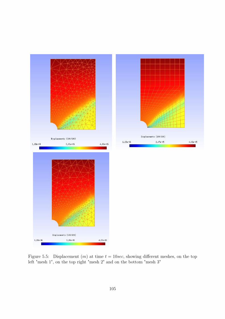
Figure 5.5: Displacement (m) at time t = 10sec, showing different meshes, on the topleft "mesh 1", on the top right "mesh 2" and on the bottom "mesh 3"

105

Figure 5.6: Strain at time t = 10sec, showing different meshes, on the top left "mesh 1",on the top right "mesh 2" and on the bottom "mesh 3"

106

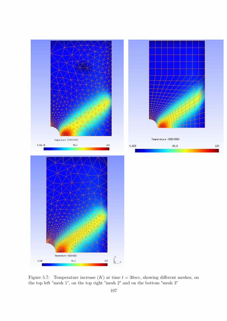
Figure 5.7: Temperature increase (K) at time t = 30sec, showing different meshes, onthe top left "mesh 1", on the top right "mesh 2" and on the bottom "mesh 3"

107

Figure 5.8: Displacement (m) at time t = 30sec, showing different meshes, on the topleft "mesh 1", on the top right "mesh 2" and on the bottom "mesh 3"

108

Figure 5.9: Strain at time t = 30sec, showing different meshes, on the top left "mesh 1",on the top right "mesh 2" and on the bottom "mesh 3"

109

Figure 5.10: Evolution of reaction (in N) function of displacement (in m), for the threedifferent meshes

Figure 5.11: Reference solution of the 2D thermo-visco-elastic problem, temperatureincrease (K) at t = 5s

110

Figure 5.12: Reference solution of the 2D thermo-visco-elastic problem, strain evolutionat t = 5s

Figure 5.13: Reference solution of the 2D thermo-visco-elastic problem, temperatureincrease (K) at t = 30s

111

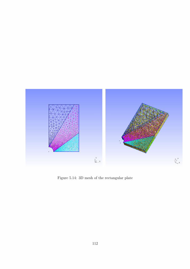
Figure 5.14: 3D mesh of the rectangular plate

112

Figure 5.15: Temperature increase (K) at time t = 50s

113

Figure 5.16: Evolution of strain for time t = 50s

114

Figure 5.17: Zoom on the strain field at time t = 50s

115

0 0.1 0.2 0.3 0.4True Strain

0

200

400

600

800

1000

True

Stre

ss [M

Pa]

ExperimentalSimulation

Al2024-T3

Figure 5.18: Stress-strain curve for rate-independent 2023-T3 aluminum alloy

116

0 0.1 0.2 0.3 0.4Plastic Strain

0

10

20

30

40

50

Tem

pera

ture

incr

ease

[K]

Exp. (quasistatic)Exp. (dynamic)Simulation

Al2024-T3

Figure 5.19: Adiabatic heating curve for rate-independent 2023-T3 aluminum alloy

117

Figure 5.20: Necking of a rectangular bar, the center of the bar corresponds to the axesorigin

118

Initial conditions The rectangular plate is supposed having a uniform temperatureat t = 0s of value 293K, the initial condition are given by

u(0) = 0 m

u(0) = 0 m.s−1

θ(0) = 0K

θ(0) = 0K.s−1

(5.21)

Mesh The choice of mesh is critical in numerical simulation designs. In addition tothat it affects the computational cost, it affects also the precision of the obtained results.The mesh is applied, by symmetry, on the eighth of the plate. This is given by figure5.21

Figure 5.21: Mesh chosen for the simulation, necking of a rectangular bar

Adaptive time step The chosen time step follows the same rule as previous applica-tion, that is given by table 5.3, and algorithmic parameters have been chosen as follows:

1. ∆tmax = 1 sec

2. ∆tmin = 10−6 sec

3. Maximum number of iterations = 20

119

Figure 5.22: Appearance of an inhomogeneity of the temperature field caused by theconvective boundary conditions (figure on the right), although the deformation is ho-mogenous (figure on the left) for a simulation time close to 0.5s

5.3.3 Results

Although the deformation, and thus the associated heating, is initially completely ho-mogeneous, heat exchange with the environment quickly creates an inhomogeneity inthe temperature field (see figure 5.22 at a time close to 0.5s).

Note that the temperature variation in the rod is initially negative, because thermo-elastic effects (thermal expansion) dominate at this stage.

The results given by figures 5.23 5.24 and 5.25 shows the displacement, equivalent plasticstrain and the temperature field for a time t = 40s. We can see clearly that despite theabsence of initial geometric defects, the deformation gradually localizes in the middle ofthe bar, leading to its necking.The inhomogeneity in the temperature field (although it is initially low) leads to the soft-ening of elastic and plastic mechanical properties, which in turn causes an inhomogeneityin the mechanical field (total and plastic deformation).

5.3.4 Algorithmic analysis

As done in previous applications, we will summarize and comment the efficiency of thealgorithms that we have described so far.

120

Figure 5.23: Displacement field (m) for t = 40s, see figure (5.24)

Table 5.15 summarizes the results of each algorithmic scheme, the simulation is donewith a precision equal to 10−8 and is run for 15s of total simulation time.

Table 5.15: Comparison between the three algorithmic schemes, with a precision of 10−8

and a simulation time of 15 s

Algorithm Total iteration number Elapsed computational time

Newton 51 2min 38s

Alternate 58 8m 45s

Uzawa 1 90 −Uzawa 2 112 20m 47s

Modified Uzawa 3 1161 1h 49m 52s

Uzawa 4 1052 −

121

Figure 5.24: Equivalent plastic strain for t = 40s, localization of deformation that resultsfrom convective boundary conditions

Table 5.15 show an important result, Newton scheme seem to reduce the total iterationnumber and time cost, whereas Uzawa-like algorithms (that dominated Newton’s in thethermo-visco-elastic application), seem to be much less efficient.When running the simulation, the softening mechanism of mechanical properties, andthus total and plastic deformation seem to affect more and more the simulation cost fort beyond 15s, where the algorithmic schemes execute more iterations to converge. Forthis we show the limitation of some algorithms, and the deterioration of others.

Table 5.16 shows the limitation of the alternated algorithm and Uzawa 2, while Newtonscheme exhibit the best computational cost.

5.3.5 Conclusion

In this application we have applied the variational formulation to an example consideringthe traction of a rectangular rod, with an elasto-plastic behavior, leading to its neckingdue to the inhomogeneity of the temperature field.Different algorithmic schemes have been applied, in particular Newton, Alternated and

122

Figure 5.25: Temperature increase (K) for t = 40s, localization of temperature thatresults from convective boundary conditions

Table 5.16: Limitation of different algorithmic schemes, simulation is ran with a precisionof 10−8 and a simulation time of 40s

Algorithm Total iteration number

Newton 2437Alternate Limitation at t = 17s

Uzawa 1 Limitation at t = 19s

Uzawa 2 Limitation at t = 18.4s

Modified Uzawa 3 7854Uzawa 4 6742

Uzawa-like scheme (as described previously).An important conclusion can be extracted through this application, is that Uzawa-scheme that used to exhibit the best performance between the three schemes in the

123

case of thermo-visco-elastic application, seems to loose its role in this case, and Newtonscheme has acceded to the throne.We can therefore deduce that there is no absolute scheme that exhibits best perfor-mance. Therefore according to the type of coupling, the use of Newton, Uzawa-like orthe alternated scheme can behave differently.

124

Conclusion and Perspective

As we have discussed throughout this manuscript, thermo-mechanical coupling in ma-terials is due to multiple effects such as thermo-visco-elasticity, visco-plasticity, viscousdissipation, dependence of mechanical characteristics on temperature (and so on...) Nu-merical simulations of these kind of coupling is challenging, especially when a strongcoupling effect is present.

We have exposed throughout this work that algorithmic approaches found in the en-gineering literature of coupled problems fall within two alternative strategies, the mono-lithic or simultaneous solution scheme that consists of resolving simultaneously mechan-ical and thermal balance equation, and staggered schemes, in which the coupled systemis partitioned therefore the mechanical and thermal problems are solved alternatively.

The main objective of this work was the validation, analysis and improvement of mono-lithic algorithmic schemes via an energy-consistent variational formulation of coupledthermo-mechanical problems. Note that the presented formulation does not include me-chanical inertial effect, but transient thermal effects are taken into account. However,they appear dependent on the loading rate, the problem keeps the form of a quasi-stationary problem. The variational approach has many advantages (see chapter 4),especially that it leads to a symmetric numerical formulation, thus overcoming the disad-vantages of classical monolithic strategies that often lead to non-symmetric formulations.

Since the variational formulation allows to write mechanical and thermal balance equa-tion under the form of an optimization problem of a scalar energy-like functional, differ-ent optimization algorithmic schemes were used, the classical Newton-Raphson scheme,the alternated algorithm, and Uzawa-like algorithms.We recall briefly that alternated scheme consists in minimizing with respect to displace-ment, at a constant temperature, then maximizing with respect to temperature at aconstant displacement until convergence, while Uzawa-like scheme consists of limitingthe maximization on the temperature to only one iteration (see chapter 4).

To show the validation of the energetic formulation, and compare the efficiency of differ-ent algorithms, various applications of coupled thermo-mechanical problems have beenexposed in details, such as thermo-visco-elastic strong coupled problem from a simplifiedproblem consisting of an infinitesimal control volume to a more general 2D and 3D cou-

125

pled thermo-elastic boundary-value problem, and then another application of a neckingin a bar with an thermo-elasto-plastic coupling.In all cases the effects of heat capacity, intrinsic dissipation and the heat exchange withthe environment are included in the model.

The simplified case, showed that all three algorithms exhibit good performance, butUzawa-like algorithms seem to reduce the global time cost then the two others.After many test, we also showed that the solution of the scalar energy-like functional isa saddle point. Note that this results motivated us to use specific algorithms, such asUzawa scheme.

The results of a more general 2D thermo-visco-elastic problem shows an evolution andpropagation of a localized deformation zone that is accompanied by a localized temper-ature zone. A reference solution validated the obtained results.Although Newton exhibits good performance in the beginning, it encounters convergencedifficulties when coupling becomes stronger and localization develops, causing the limi-tation of the scheme. This limitation is caused by the non-convergence at the minimaltime step allowed. The alternated scheme offers more interesting results since it hasovercome the limitation for low precision, and allows better performance at higher ones.Uzawa scheme encounters some problems of convergence, on top of that the extraction ofsub-matrices from the total matrix influences considerably the time cost. Therefore wedecided to proceed in another manner by treating at first the thermal problem, and thenthe mechanical problem by limiting the minimization of the displacement field to one it-eration. This approach seems to reduce more the global time cost and iteration numbers.

Eventually, the variational formulation is applied to the example of traction of a rectan-gular rod, with an elasto-plastic behavior, leading to its necking due to the inhomogeneityof the temperature field.An interesting result is concluded, Uzawa-scheme that used to exhibit the best perfor-mance between the three schemes in the case of thermo-visco-elastic application, seemsless efficient in this application, while Newton scheme exhibits good performance byovercoming the limitation of other schemes and performs with a better computationalcost. This might due to the different types of coupling in each problem, recalling thatwe have considered a brutal transition for mechanical coefficients with respect to tem-perature in the visco-elastic model, whereas in the elasto-plastic application, mechanicalproperties are set constants and thermo-plastic properties (Yield stress dissipated) aremodeled with a smoother transition.

Through those various applications, we have showed the capacity of the energy-consistentvariational formulation to deal with coupled problems, in addition to its encouraginggood performance. The aim of the application of different algorithmic schemes is tofind the one that exhibits best performance, and what can be concluded (through theseapplications) that there is no unique absolute scheme that achieved this task. There-

126

fore according to the type of coupling, the use of Newton, Uzawa-like or the alternatedscheme can behave differently.

Perspective It is still interesting to try to optimize the computation of Schur com-plement, since the extraction of sub-diagonal matrixes from the total matrix and theevaluation of the Schur complement deteriorates considerably the computational time.The extraction from a skyline matrix being not affordable, sparse storage may improveits evaluation, still need to test it.We can use for example an optimized system, for example MUMPS (a MUltifrontalMassively Parallel sparse direct Solver), to evaluate the Schur complement. For this wejust need to introduce KUU ,KT T , KT U and KUT in sparse matrix storage (storage of nonzero elements), and then MUMPS will evaluate the Schur complement in an optimizedway.

Another solution lays on using iterative solver instead of direct solvers. We recall thatour problem is to solve the following

[Kc]δT = −RT (5.22)

where [Kc] is given by

[Kc] = [KT T ] − [KT U ][KUU ]−1[KUT ] (5.23)

If we choose the conjugate gradient method as an iterative method, the solution of 5.22transforms into minimizing the following functional:

f(δT) = 12δTT [Kc]δT − δTT −RT (5.24)

The resulting algorithm to solve 5.22 is detailed as follow :

We set

r0 = −RT (5.25)p0 = r0 (5.26)k = 0 (5.27)

repeat

αk = rT

krk

pT

kKcpk

(5.28)

δTk+1 = δTk + αkpk (5.29)rk+1 = rk − αk[Kc]pk (5.30)

127

if rk+1 is sufficiently small then exit loop end if

βk = rT

k+1rk+1r

T

krk

(5.31)

pk+1 = rk+1 + βkpk (5.32)k = k + 1 (5.33)

end repeat

Note that α and β are scalar and pk is a vector.The computation of [Kc]pk in the algorithm will be treated as follow

[Kc]pk = [KT T ]pk − [KT U ][KUU ]−1[KUT ]pk (5.34)we set

[KUT ]pk = V (5.35)and

[KUU ]−1V = W (5.36)Is this case we obtain W by solving

[KUU ]W = V (5.37)

therefore equation 5.34 becomes

[Kc]pk = [KT T ]pk − [KT U ]W (5.38)

In this case equation 5.38 shows that the construction of the Schur complement isconstructed by an alternative way (1 solve of equation 5.37, and 3 multiplication of[Matrix] × V ectors, and eventually one addition ).Note that the use of this algorithm requires that the total matrix and therefore the Schurcomplement is a positive definite matrix.

In the chapter of application we have showed that the used of the Schur complementdoes no change dramatically the iteration numbers (if we compare Uzawa1 and Uzawa2,or Uzawa3 and 4 the performance of each algorithm is comparable), therefore it is in-teresting to try to use other methods for future work as staggered algorithms, since thebase of this work lay on the use of monolithic solution that may lead to impossibly largesystem and do not take advantage of the time scale involved in the problem.The use of the staggered strategies will overcome these drawbacks and hopefully, willlead to better computational costs. These strategies still need to be tested via variationalapproach and to be compared to monolithic solution.

128

Table 5.17: Isothermal staggered scheme

1 Predict the temperature field zthermal(t = t

k+1) = zthermal(t = t

k)

2 Solve for the mechanical field infϕn+1

Φ∗∗n

(ϕn+1, T

p

n+1)

3 Which provides zmechanical(t = t

k+1)

4 Correct the temperature field supTn+1

Φ∗∗n

(ϕn+1, Tn+1)

5 Which provides zthermal(t = t

k+1)

6 Compute velocity, acceleration ϕ, ϕ and H

and flux fields

7 Move to next step t = t + ∆t

Isothermal staggered scheme This scheme partitions the thermo-mechanicalproblem (without a fixed point) according to different coupled field (displacement andtemperature), and the different optimization algorithms may be applied to each parti-tion. In variational form we can write it as

infϕn+1

Φ∗∗n

(ϕn+1, T

p

n+1)

supTn+1

Φ∗∗n

(ϕn+1, Tn+1)

In this case the phase 1 is solved by an optimization algorithm (say Newton-Raphson),followed by phase 2 where we may apply another optimization algorithm (and anotherdiscretization and time increment if we wish) then we move to the next time step with-out verifying the balance equations.This scheme is summarized in table

Adiabatic staggered scheme This scheme partitions the problem into two:The first phase is an adiabatic elasto-dynamic phase where the entropy is held constant,followed by a heat conduction phase at constant mechanical configuration. In variational

129

Table 5.18: Adiabatic staggered scheme

1 Solve for the local adiabatic problem infϕn+1

supT

A

n+1

Φ∗∗n

(ϕn+1, T

A

n+1) where χ(Gn+1) is ignored

2 Which provides ϕ and TA

3 Correct the temperature field supTn+1

Φ∗∗n

(ϕn+1, Tn+1)

4 Which provides zthermal(t = t

k+1)

5 Compute velocity, acceleration ϕ, ϕ and H

and flux fields

6 Move to next step t = t + ∆t

form, this is given by :

infϕn+1

supT

A

n+1

Φ∗∗n

(ϕn+1, T

A

n+1) where χ(Gn+1) is ignored

supTn+1

Φ∗∗n

(ϕn+1, Tn+1)

Note that the phase 1 feature a local adiabatic problem where the temperature as thislevel is an internal variable. The phase 2 is like the isothermal staggered scheme wherethe optimization algorithm is applied on the temperature field at a constant mechanicalconfiguration. The staggered scheme is summarized in table 5.18

130

Conclusion générale

Comme nous l’avons vu tout au long de ce manuscrit, les sources de couplage thermomé-canique dans les matériaux viscoélastiques sont multiples : thermo-élasticité, dissipationvisqueuse, évolution des caractéristiques mécaniques avec la température. La simulationnumérique de ces couplages en calcul des structures présente encore un certain nombrede défis, spécialement lorsque les effets de couplage sont très marqués (couplage fort).De nombreuses approches algorithmiques ont été proposées dans la littérature pour cetype de problème. Ces méthodes vont des approches monolithiques, traitant simul-tanément l’équilibre mécanique et l’équilibre thermique, aux approches étagées, traitantalternativement chacun des sous-problèmes mécanique et thermique. La difficulté estd’obtenir un bon compromis entre les aspects de précision, stabilité numérique et coûtde calcul.

Récemment, une approche variationnelle des problèmes couplés a été proposée par Yanget al. , qui permet d’écrire les équations d’équilibre mécanique et thermique sous la formed’un problème d’optimisation d’une fonctionnelle scalaire. Cette approche variationnelleprésente notamment les avantages de conduire à une formulation numérique à structuresymétrique, et de permettre l’utilisation d’algorithmes d’optimisation.

L’objectif principal de ce travail était la validation, l’analyse et l’amélioration des sché-mas algorithmiques monolithique par une approche énergétique variationnelle pour leproblème thermo-mécanique couplé. A Noter que la formulation présentée n’inclut pasles effets d’inertie mécanique, mais les effets thermiques transitoires sont pris en compte.Cependant, ils apparaissent sous la forme d’une dépendance à la vitesse de chargement,le problème à résoudre apparait comme un problème quasi-stationnaire et non-linéaire.A noter que l’équation d’équilibre thermique utilisée ici est basée sur un bilan d’entropiecalculé sur l’incrément temporel en cours, alors que les approches classiques sont baséessur une équation d’équilibre des flux instantanés.

L’approche variationnelle présente de nombreux avantages (voir chapitre 4), surtoutqu’elle conduit à une structure symétrique, évitant ainsi les inconvénients des stratégiesmonolithiques classiques qui conduisent souvent à des formulations non-symétriques.Comme la formulation variationnelle permet d’écrire les équations d’équilibres mécaniqueet thermique sous la forme d’un problème d’optimisation d’une fonctionnelle scalaire, dif-férent algorithmes d’optimisation ont été utilisés tel que, le schéma de Newton-Raphson

131

classique, un schéma d’optimisation alternée, et des algorithmes de type Uzawa.On rappelle que, la procédure de l’algorithme alterné consiste à effectuer successivementdes minimisations (maximisations) par rapport au déplacement (température), tout engardant la température (déplacement) constante, jusqu’à convergence. Tandis que lesschémas de type Uzawa consistent à limiter la maximisation sur la température (ou laminimisation sur le déplacement) à une seule itération.

Pour montrer la validation de la formulation énergétique variationnelle, et comparerl’efficacité de différents schémas algorithmiques, différents problèmes de couplage thermo-mécaniques ont été exposé en détails, allant d’un problème simplifié consistant en unvolume élémentaire de matière, à des problèmes plus généraux aux conditions aux limites(2D et 3D), avec des comportements thermo-visco-élastique ou élasto-plastique. Danstous les cas, les effets de capacité thermique, de dissipation intrinsèque et d’échange dechaleur avec l’environnement sont inclus dans le modèle.

Le cas simplifié, a montré que les trois algorithmes offrent une bonne performance,mais les algorithmes de types Uzawa semblent réduire le plus le coût du temps global decalcul. De même, on obtient un second résultat intéressant que la fonctionnelle présentetoujours un point de selle dans chaque cas envisagé.Le problème thermo-visco-élastique aux conditions limites (2D et 3D) montre une évo-lution et propagation d’une zone de déformation localisée qui est accompagné par unezone de localisation de température . Les résultats sont comparés à une solution deréférence, qui valide bien l’approche variationnelle.

Bien que le schéma de Newton offre une bonne performance au début, il rencontredes difficultés de convergence lorsque la température atteint la zone de transition (fortevariation des modules élastique et visqueux) et la localisation se développe, causant lalimitation du schéma. Cette limitation est due à la non-convergence du schéma au pas detemps minimal défini par défaut. Le schéma alterné offre des résultats plus intéressantssurtout qu’il surmonte la limitation observée avec le schéma de Newton pour des faiblesprécisions, et permet un meilleur rendement pour des tolérances plus importante. Enfin,on applique le schéma de type Uzawa. Des difficultés ont été rencontrées à cause del’extraction des sous-matrices de couplage de la matrice tangente, de plus l’évaluationdu complément de Schur influence considérablement le temps de calcul global.Un deuxième type d’algorithme de type Uzawa qui consiste à limiter la minimisationsur le champs de déplacement à une seule itération a également été étudié. Ce dernierschéma semble réduire le coût global du temps de calcul.

Finalement, l’approche variationnelle est appliqué au problème de déclenchement ther-mique de la striction d’un barreau rectangulaire, avec un comportement élasto-plastique.Les différents algorithmes ont été appliqués afin de tester leurs performances. L’agorithmede Newton semble offrir les meilleurs performance dans ce cas. Rappelons que pour ceproblème, le type de couplage est différent du problème précédent où on a considéré une

132

transition brutale des coefficients mécaniques par rapport à la température, or pour ceproblème de striction de la barre, les propriétées mécaniques évoluent progressivementpar rapport à la température.

Grâce à ces différentes applications, nous avons montré la capacité de l’approche varia-tionnelle énergétique de traiter les problèmes multiphysiques couplés, ainsi que sa bonneperformance. L’application des différents schémas algorithmiques a pour but de com-parer les performances que chacun peut offrir, et ce qui peut être conclu est qu’il n’existepas de schéma absolu unique qui a des meilleurs performances indépendament du typedu problème. Ainsi, selon le type de couplage, l’utilisation d’un schéma ou un autrepeut se comporter différemment.

133

Appendix A

Stability overview

We have already exposed in chapter 3 two types of time stepping method, the mono-lithic scheme that lead to unconditional stability if we use an implicit scheme, and thestaggered algorithms that are designed to overcome the large system obtained by simul-taneous schemes, but this is often at the sacrifice of unconditional stability.

In this paragraph we will expose a quick overview about stability analysis of differ-ent schemes as exhibited by Simo and Miehe [108] , for this we consider, for simplicity, acoupled non-linear thermo-elastic problem as defined in chapter 3, in which the resultsare generalizable to other coupled problems.We recall that the thermo-elastic problem, neglecting inertial forces, can be writtenunder the following form (see section 3.6.2)

X (t) = AX (t) (A.1)

where

X (t) =

u(t)v(t)θ(t)

(A.2)

AX (t) =

v

1ρ0

∇·

C : (∇su − θα)

1c∇ ·

K · ∇θ

− 1

cα : C : ∇s

v

(A.3)

The linearized thermo-elastic problem is called stable if it inherits the contractivityproperty. In numerical analysis context, an algorithm inherits the contractivity property[108, 8, 14, 18] if

12

d

dtX (t)2 = 1

2d

dt

< X (t), X >

=< AX , X >≤ 0 (A.4)

134

where< AX , X >=

ΩX A.X dV (A.5)

Where X and AX are given by equation A.2 and A.3 given in chapter 3 (section appli-cation to a thermo-elastic problem).

The norm is given by

X (t)2 =< X , X >=

Ω

∇s

u : C : ∇su + ρ0v.v + cθ

2

dV (A.6)

A.1 Monolithic scheme

What we have developed so far (see chapter 3 section application) monolithic or simul-taneous solution.To verify the contractivity property of the thermo-elastic problem, equation A.4 shallbe satisfied

< AX , X >=

Ω

∇sv : C : ∇s

u + ρ01ρ0

div

C : (∇s

u − θα)

.v

+c1c

div (K.∇θ) − α : C : ∇s

v

θ

dV

(A.7)

Where

Ω

∇s

v : C : ∇su − α : C : ∇s

v

dV =

Ω∇s

v : C : (∇su − θθα) dV = 0 (A.8)

and

Ωdiv

C : (∇s

u − θα)

.vdV = −

Ω∇s

v : C : (∇su − θθα) dV +

δΩ

C : (∇s

u − θα)

.ndA = 0(A.9)

Equations A.8 and are the result of divergence theorem, which correspond to the cance-lation of thermal stresses and the structural elastic heating terms taking place in thoseequations. Therefore, equation A.10 becomes

< AX , X >=

Ωdiv (K.∇θ) dV = −

Ω∇θK∇θdV +

δΩθ (K∇θ) ndA (A.10)

Where

δΩθ (K∇θ) ndA = 0 Homogeneous boundary condition

then< AX , X >=

Ωdiv (K.∇θ) dV = −

Ω∇θK∇θdV ≤ 0 (A.11)

Equation A.11 is the proof of contractivity of A, therefore the simultaneous solutionscheme inherit the contractivity property, therefore it is unconditionally stable. Equa-tion A.11 shows that energy lost is due to conductivity.

135

A.2 Isothermal split

The coupled problem is now split into two operators, the first one where the temperatureis held constant, and the second purely thermal phase where the mechanical configuration(displacement) is held constant. This split is known as the isothermal staggered splitthat can be written as follow

A = A1 + A2 (A.12)Where

A1X =

v

1ρ0

div

C : (∇s

u − θα)

0

Problem 1: mechanical phase at a fixed temperature

(A.13)

A2X =

001cdiv

K.∇θn+α

− 1

cα : C : ∇s

v(n+α) or (n+1)

Problem 2: Heat conduction phase

(A.14)It has been shown [108] that the admissible isothermal split of the problem of evolutiondoes not define sub-problems which inherit the contractivity property of the originalproblem (A1 cannot generate a quasi-contractive semigroup, thus breaking the contrac-tive structure of the original problem), thus there is no guarantee of stability for thestaggered isothermal phase.

A.3 Adiabatic split

Now the coupled thermo-elastic problem is split into another two operators, where thefirst is an adiabatic elasto-dynamic phase, which the entropy of the system is heldconstant, and the second one is a heat conduction phase at fixed configuration, this iswritten as

A1X =

v

1ρ0

div

C : (∇s

u − θα)

− 1cα : C : ∇s

u

Problem 1: Elasto-dynamic phase (A.15)

136

A2X =

001cdiv

K.∇θn+α

Problem 2: Heat conduction phase (A.16)

The inner product of the two operators is given by

A1X , X = 0 (A.17)

andA2X , X = −

Ω∇θ.K.∇θdV ≤ 0 (A.18)

We can remark that the adiabatic mechanical phase preserves the total energy of thesystem (A1 is an operator with no dissipation), whereas the dissipation in the heatconduction phase is the same as in the coupled problem, therefore the adiabatic splitpreserves the contractivity property, rendering the scheme unconditionally stable.

A.3.1 Limitation of the adiabatic staggered scheme

Although the adiabatic scheme is cited as the ultimate solution of instability that maybe encountered after the use of isothermal staggered scheme, adiabatic staggered schemeis limited for a random time discretization and presence of a strong coupling. In fact,thisscheme has the features of unconditional instability when considering time discretizationcharacterized by a constant time step [114].Therefore, it cannot be always limited with such type of discretizaton, especially whileimplementing a general software for coupled thermo-mechanical problems.

Adam [114] has illustrated this phenomenon by considering a simple case consistingof a traction of an axisymmetric element with a thermo-elastic behaviour. Figure A.1show the evolution of the temperature of the upper side.

Time discretization is caracterized by constant time step except between 4.9 and 5 sec

where it is added an additional time at t = 4.999 sec.Is is thus found in this moment with two consecutive time steps of very different sizes,an error of evaluation of the temperature field when using the adiabatic scheme.Similarly, of a given fraction where (∆t)n−1

(∆t)n

= 1, the evolution error of temperature ismore important at the presence of strong coupling.On the other hand this phenomenon does not appear when using a constant time step ,as in the case illustrated by Armero and Simo [108]

137

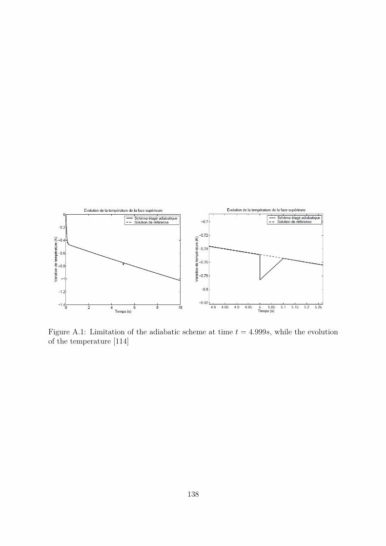
Figure A.1: Limitation of the adiabatic scheme at time t = 4.999s, while the evolutionof the temperature [114]

138

Appendix B

Complementary results for the

thermo-visco-elastic behaviour of a

rectangular plate with a hole in 2D

plane

In this annex we will show the complementary results of thermo-visco-elastic behaviourof a rectangular plate with a hole in 2D plane, as described in chapter 5 (section 5.1). InThese complementary results, we show the results of Velocities and Heat Flux for time10s and 30s.

139

Figure B.1: Velocities (m.s−1) at time t = 10sec, showing different meshes, on the top

left "mesh 1", on the top right "mesh 2" and on the bottom "mesh 3"140

Figure B.2: Heat flux (W.m−2) at time t = 10sec, showing different meshes, on the top

left "mesh 1", on the top right "mesh 2" and on the bottom "mesh 3"

141

Figure B.3: Velocities (m.s−1) at time t = 30sec, showing different meshes, on the top

left "mesh 1", on the top right "mesh 2" and on the bottom "mesh 3"142

Figure B.4: Heat flux (W.m−2) at time t = 30sec, showing different meshes, on the top

left "mesh 1", on the top right "mesh 2" and on the bottom "mesh 3"

143

Bibliography

[1] E. Fancello J. Ponthot and L. Stainier. A variational formulation of constitutivemodels and updates in non-linear finite viscoelasticity. Computational Methods inApplied Mechanics, 65:1831–1864, 2006. 71

[2] Geankoplis, Christie John (2003) Transport processes and separation process prin-ciples : (includes unit operations) (4th ed. ed.). Upper Saddle River, NJ: PrenticeHall Professional Technical Reference. ISBN 0-13-101367-X 20

[3] J.D. Achenbach. Wave Propagation in Elastic Solids,5th printing, North Holland,Amesterdam 1987.

[4] J. Lemaitre and J.-L. Chaboche. Mécanique des matériaux solides. 1985. 34, 52

[5] J.H. Argyris and J. St. Doltsinis. On the natural formulation and analysis of largedeformation coupled thermo-mechanical problems’, Computer Methods in AppliedMechanics and Engineering, 25, 195-253, 1981. 51

[6] M. Ortiz, L. Stainier, 1999. The variational formulation of viscoplastic constitutiveupdates. Comput. Methods Appl. Mech. Eng. 171 (3-4), 419-444. 69

[7] K.C.Park; C.A. Felippa and J.A.DeRuntz. Stabilization of staggered solution pro-cedures for fluid-structure interaction analysis. Computational Methods for Fluid-Structure Interaction Problems, 26:94–124, 1977. 51

[8] J. M. Ball and G. Knowles. ’Lyapunov functions for thermomechanics with spatiallyvarying boundary temperatures’, Arch. Rational Mech. Anal., 92, 193-204, 1986. 134

[9] K.C. Park and C.A. Felippa. Computational methods in transient analysis. InT. Belytschko and T.J.R Hughes, editors, Partitioned analysis of coupled problems,North-Holland, Amesterdam, 1983. 42, 51

[10] P. A. C. Raats « Steady Gravitational Convection Induced by a Line Source of Saltin a Soil », in Soil Science Society of America Journal, no 33, 1969, p. 483-487 22

[11] D.E. Carlson ’Linear Thermoelasticity’, in S. Fluegge (ed.), Handbuch der Physik,Bd. VI/2a, Springer-Verlag, Berlin, 172, pp. 297-346.

144

[12] Z. Tonkovic, J. Soric, and W. Kratzig. ’On nonisothermal elastoplastic analysis ofshell components employing realistic hardening responses.’ International Journal ofSolids and Structures, 38:5019-5039, 2001. 34

[13] I. Klotz, R. Rosenberg, Thermodynamics - Basic Concepts and Methods, 7th ed.,Wiley (2008) 24

[14] C.M. Dafermos, ’Contraction semigroups and trend to equilibrium in continuummechanics’, Springer Lecture Notes in Mathematics 503, 1976, pp. 295-306. 134

[15] A. Rosakis J. Hodowany, G. Ravichandran and P. Rosakis. Partition of plastic workinto heat and stored energy in metals. Experimental Mechanics, 40(2):113–123, 2000.102

[16] I. St. Doltsinis, ’Aspects of modelling and computation in the analysis of metalforming’, Eng. Computat., 7, 2-20, 1990.

[17] P. Duhem, Traité d’Energetique ou de Thermodynamique Générale, Gauthier Vil-lars, Paris, 1911.

[18] J. L. Ericksen, ’Thermoelastic stability’, Proc. 5th National Cong. on AppliedMechanics, 1966, pp. 187-193. 134

[19] K. C. Park Partitioned transient analysis procedures for coupled-field problems:accuracy analysis, J. Appl. Mech., 47, 370-376, 1980. 6

[20] M. A. Biot, 1956. Thermoelasticity and irreversible thermodynamics. J. Stat. Phys.27, 250-253. 69

[21] K. C. Park and C. A. Felippa, Partitioned transient analysis procedures for coupled-field problems: accuracy analysis, J. Appl. Mech., 47, 919-926, 1980. 6

[22] M. E. Gurtin, ’Thermodynamics and stability’, Arch. Rational Mech. Anal, 59,53-96, 1975.

[23] W. Han, S. Jensen, B.D. Reddy, 1997. Numerical approximations of problems inplasticity: error analysis and solution algorithms. Numer. Linear Algebra Appl. 4,191-204. 69

[24] K. C. Park and C. A Felippa, ’Partitioned analysis of coupled problems’, in T.Belytschko and T.J.R Hughes (eds.) Computational Methods in Transient Analysis,North Holland, Amsterdam, 1983. 6, 51

[25] H. Parkus. Thermoelasticity, 2nd edn, Springer -Verlag, Wien, 1976.

[26] Han, W., Reddy, B.D., Schroeder, G.C., 1997. Qualitative and numerical analysisof quasi-static problems in elastoplasticity. SIAM J. Numer. Anal. 34, 143-177. 69

145

[27] J.J. Aklomis and W.J. Mackwright. Introduction to polymer visco-elasticity. Wileyinterscience, second edition edition, 1983. 81

[28] B. Halphen and Q. Nguyen. Sur les matériaux standard généralisés. Journal demécanique, 14:39–63, 1975. 31, 70

[29] J. C. Simo ’Algorithms for static and dynamic mutiplicative plasticity that preservethe classical return mapping schemes of the infinitesimal theory’, ComputationalMethods in Applied Mechanics and Engineering, 1991 101

[30] J. C. Simo and C. Miehe. Associative coupled thermoplasticity at finite strains:Formulation, numerical analysis and implementation’ Computational Methods inApplied Mechanics and Engineering 49, 101

[31] O. C. Zienkiewicz, D. K. Paul and A. H. Chan, Unconditionally stable staggeredsolution procedure for soil-pore fluid interaction problems Computational Methodsin Applied Mechanics and Engineering, 26, 1039-1055, 1988. 6, 42, 51

[32] J.T. Oden and W.H. Armstrong, ’Analysis of Nonlinear Dynamic Coupled Thermo-viscoelasticity Problems by the Finite Element Method’, Computers and Structures,Vol. 1, pp. 603-621, 1971. 6, 42

[33] W. K. liu and H. G. Chang, ’A Note on Numerical Analysis of Dynamic CoupledThermoelasticity’ Computational Methods in Applied Mechanics and Engineering,Vol. 50, 1033-1041, 1983.

[34] V. I. Danilovskaya, On a Dynamical Prolem of Thermoelasticity, PrikladnayaMatematika i Mechanika, Vol. 13,No 3, pp. 341-344, 1952.

[35] G. I. Taylor and H. Quinney. ’ The latent heat remaining in a metal after coldwork.’ Proc. of the Royal Society, A163:157-181, 1937. London. 34

[36] J. C. Simo. ’Nonlinear stability of the time discrete variational problem in nonlinearheat conduction and elastoplasticity’, Computational Methods in Applied Mechanicsand Engineering 88, 111-131, 1991.

[37] Y. Dubois-Pelerin, ’Linear Thermomechanical Coupling by the Staggered Method’,IREM Internal report, Ecole Polytechnique Federale de Lausanne, 1989. 6

[38] M. Zhou, G. Rachivadran, and A. J. Rosakis. Dynamically propagating shear bandsin impact-loaded prenotched plates - II : numerical simulations. Journal of Mechanicsand Physics of Solids, 44:1007-1032, 1996. 34

[39] K. C. Park, C. A. Felippa and J. A DeRuntz "Stabilization of Staggered SolutionProcedures for Fluid-Structure Interaction Analysis", Computational Methods forFluid-Structure Interaction Problems, ed. by Delytshcko and Geers, ASME AppliedMechanics Symposia Series, AMD, 26, 94-124, 1977 42, 51

146

[40] M.Kleiber P. Wriggers, C. Miehe and J.C. Simo. Computer methods in appliedmechanics and engineering (complas 2). In E. Hinton Owen and E. Oñate, editors,On the coupled thermo-mechanical treatment of necking problems via FEM, pages527–542, Barecelona, Spain, 1983. Pineridge Press. 100

[41] K.C.Park and C.A.Felippa. Computational methods in transient analysis. In T. Be-lytschko and T.J.R Hughes, editors, Partitioned analysis of coupled problems, North-Holland, Amesterdam, 1983. 42, 49

[42] K. C. Park, "Partitioned Transient Analysis Procedure for coupled-Field Problems:Stability Analysis" J. Appl. Mech., Vol. 47, No. 2, pp.370-376, 1980 6, 42

[43] R. E. Nickell and J.L. Sackman, "The Extended Ritz Method Applied to Tran-sient Coupled Thermoelastic Boundary-Value Problems", Rep. No. 67-3, Structuresand Materials Research, University of California at Berkeley, 1967. Linear CoupledThermoelasticity, J. Appl. Mech., Vol. 35, PP. 255-266, 1968 6

[44] N.Charalambakis, 2011. Shear Stability and Strain, Strain-rate and TemperatureDependent ’Cold’ Work. International Journal of Engineering Science 39 (17), 1899-1911. 39, 100

[45] J. Fourier Théorie analytique de la chaleur, Paris, 1822 21

[46] S. R. Chen and G. T. Gray, 1996. Constitutive behavior of tantalum and tantalum-tungsten alloys. Metallurgical and Materials Transactions A 27 (10), 2994-3006.100

[47] Y. Bamberger Mécanique de l’ingénieur, Tome II, Ed. Hermann, Paris, 1981 17

[48] B. Halphen and Q. S. Nguyen Sur les matériaux standards généralisés, Journal deMécanique, Vol. 14, pp. 39-63, 1975 17

[49] J. L. Nowinsky Theory of thermoelasticity, Noordhoff International, Alphen aanden Rijn, 1978.

[50] J.C. Simo and C. Miehe. Associative coupled thermoplasticity at finite strains :Formulation, numerical analysis and implementation. Computer Methods in AppliedMechanics and Engineering, 98:41–104, 1992. 34, 100

[51] J. J. Aklomis and W. J. Machwright Introduction to polymer viscoelasticity, 2nd

editions, Wiley interscience, 1983.

[52] A. Monlinari and R. J. Clifton Analytical characterization of shear localization inthermoviscoplastic materials, Journal of Applied Mechanics, 54, 806-812, 1987.

[53] D. Assaker. Analyse thermomécanique non-linéaire par éléments finis des traite-ments thermiques des métaux. PhD. thesis, Université de Liège, 1989-90. 101

147

[54] M. Biot. In proceedings of the third us national congress of applied mechanics.In ASME, editor, Linear thermodynamics and the mechanics of solids, pages 1–18,1958.

[55] G. A. Maugin. The thermomechanics of nonlinear irreversible behaviors, volume27 of Series on Nonlinear Science. World Scientific leon o. chua edition, 1999. 71

[56] J. Mandel Cours de mécanique des milieux continus, Gauthier-Villard, Paris, 1966.27

[57] B. Booley and J. Weiner. Theory of thermal stresses. Wiley, 1960. 17

[58] O.T Bruhms, H. Xiao and A. Meyers. A self-consistent eulerian rate type modelfor finite deformation elasto-plasticity with isotropic damage. International Journalof Solids and Structures, 38: 657-683, 2001. 31

[59] A. Chrysochoos. Bilan énergétique en élastoplasticité grandes déformations. Journalde mécanique théorique et appliqué, 4(5) :589-614, 1985. 101

[60] A. Chrysochoos and R. Peyroux. Analyse expérimentale et modélisation numériquedes couplages thermomécanique dans les matériaux solides. Revue générale de ther-momécanique, 37: 852-606, 1998. 101

[61] M. Ortiz and L. Stainier. The variational formulation of viscoplastic constitutiveupdate. Computational Methods in Applied Mechanics, 171:419–444, 1999. 6

[62] J. Vassoler E. Fancello and L. Stainier. A variational constitutive update algo-rithm for a set of isotropic hyperelastic-viscoplastic material models. ComputationalMethods in Applied Mechanics, 197:4132–4148, 2008. 71, 101

[63] M. G. Cooper, B. B. Mikic and M. M. Yovanovich. Thermal contact conductance.International Journal of Heat and Mass Transfer, 12: 279-300, 1969. 7121

[64] M. A. Biot, 1958. Linear thermodynamics and the mechanics of solids. In: Pro-ceedings of the Third US National Congress of Applied Mechanics. ASME, pp. 1-18.69

[65] G. Batra, 1989. On a principle of virtual work for thermo-elastic bodies. J. Elasticity21, 131-146. 69

[66] G. Dhatt and G. Touzot. Une présentation de la méthode des éléments finis. Col-lection Université de Compiègne, Maloine s.a. edition, 1984.

[67] P. Germain and P. Muller Introduction à la mécanique des milieux continus, Ed.Dunond, Paris, 1985 17

148

[68] M. Hogge. Modélisation des transferts de chaleur et de matière. Notes de cours -LTAS - Université de Liège. 55

[69] Unconditionally stable algorithms for nonlinear heat conduction. Computer Meth-ods in Applied Mechanics and Engineering, 10: 135-139, 1977.

[70] M. Ortiz, E. A. Repetto and L. Stainier. A theory of subgrain dislocation structruesin ductile single crystals. Journal of the Mechanics and Physics of Solids, 48: 2077-2114, 2000.

[71] P. Perzyna. Thermodynamics Theory of plasticity. In Chia-Shun Yih, editor, Ad-vances in Applied Mechanics, volume 11, pages 313-355. Academic Press, 1971. 101

[72] A. Molinari, M. Ortiz, 1987. Global viscoelastic behavior of heterogeneous ther-moelastic materials. Int. J. Solids Struct. 23(9), 1285-1300 69

[73] L. Stainier Notes relatives au cours donné à Montpellier, 2006. 49, 70, 101

[74] J.C. Simo and C. Miehe. Associative coupled thermoplasticity at finite strains :Formulation, numerical analysis and implementation. Computer Methods in AppliedMechanics and Engineering, 46:201–215, 1992. 49

[75] J. H.Lienhard (2008) A Heat Transfer Textbook (3rd ed.). Cambridge, Mas-sachusetts: Phlogiston Press. ISBN 978-0-9713835-3-1. 20

[76] J. R.Welty, C. E. Wicks and R. E. Wilson (1976) Fundamentals of momentum,heat, and mass transfer (2 ed.). New York: Wiley 21

[77] P. Radovitzky and M. Ortiz. Error estimation and adaptive meshing in stronglynonlinear dynamic problems. Computer Methods in Applied Mechanics and Engi-neering, 172: 203-240, 1999.

[78] M. Ortiz and E. A. Repetto. Nonconvex energy minimization and dislocation struc-tures in ductile single crystals. Journal of the Mechanics and Physics of Solids,47:397-462, 1999.

[79] L. Stainier. 19ème congrès français de mécanique. In Une approche variationnelledes couplages thermo-mécaniques en calcul des structures, Marseille, France, Août2009. Institut de Recherche en Génie Civil et Mécanique (GeM UMR 6183 CNRS),Ecole Centrale de Nantes. 48, 49, 70

[80] Y. Dubois-Pelerin. Linear thermomechanical coupling by the staggered method.IREM Internal Report, 1989. 42, 49

[81] Çengel, Yunus A. (2003) Heat Transfer: a practical approach. McGraw-Hill seriesin mechanical engineering (2nd ed.). 23

149

[82] G. T. Camacho and M. Ortiz. Adaptive Langrangian modeling of ballistic penetra-tion of metallic targets. Computer Methods in Applied Mechanics and Engineering,60:813-821, 1997. 34

[83] A. Chrysochoos, H. Pham and O. Maisonneuve Experimental and theoretical anal-ysis of thermomechanical coupling, extended paper related to SMIRT conference,1996. 17

[84] A. Ibrahimbegovic and L. Chorfi. Covariant principal axis formulation of asso-ciated coupled thermoplasticity at finite strains and its numerical implementation.International Journal of Solids and Structures, 39:499–528, 2002. 100

[85] M. Ortiz and L. Stainier. The variational formulation of viscoplastic constitutiveupdates. Computer Methods in Applied Mechanics and Engineering, 171: 419-444,1999. 71

[86] E. Fancello, J. P. Ponthot and L. Stainier. A variational formulation of constitu-tive models and updates in non-linear finite viscolasticity. International Journal forNumerical Methods in Engineering, 2006. 71

[87] W. K. Belvin and K. C. Park Structural tailoring and feedback control synthesis:an interdisciplinary approach, J. guidance, control & dynamics, 13, 424-429, 1990. 6

[88] G. Herrmann, 1963. On variational principles in thermoelasticity and heat conduc-tion. Q. Appl. Math. 22, 151-155. 69

[89] C. Farhat and R. X. Roux Implicit parallel processing in structural mechanics,Computat. Mech. Advances, 2, 1-124, 1994. 6

[90] D. Van Nostrand McCulloch, Richard, S. (1876) Treatise on the Mechanical Theoryof Heat and its Applications to the Steam-Engine, etc.. 24

[91] C. Farhat;Y. Dubois-Pelerin; K. C. Park. An unconditionally stable staggeredalgorithm for transient finite element analysis of coupled thermoelastic problems.NASA Contractor Report 189066, University of Colorado, Boulder Colorado, EcolePolytechnique Federale de Lausanne, November 1991. 51

[92] D.K. Paul O.C. Zienkiewicz and A. H. Chan. Unconditionally stable staggeredsolution procedure for soil-pore fluid interaction problems. International JournalFor Numerical Methods In Engineering, 88:111–131, 1991. 51

[93] A. Chrysochoos and J.C. Dupré. Proceedings of the eurotherm seminar nb. 27.In Euro Thermique, editor, An infra-red set-up for continuum thermomechanics,Quantitative Infra-Red Thermography, pages 129–134, 1992. 88

[94] F. A. Felippa Refined finite element analysis of linear and nonlinear two-dimensionalstructures, PhD Dissertation, Department of Civil Engineering, University of Cali-fornia at Berkeley, Berkeley, CA, 1966 6

150

[95] F. A. Felippa and K. C. Park. Compuational aspects of time integration proceduresin structural dynamics, Part I: Implementation, J. Appl. Mech., 45, 595-602, 1979.6

[96] Faghri, A., Zhang, Y., and Howell, J. R., 2010 Advanced Heat and Mass Transfer,Global Digital Press, Columbia, MO. 21

[97] C. A. Felippa and K. C. Park Staggered transient analysis procedures for coupledtransient analysis procedures for coupled dynamic systems: formulation, Comp.Meths. Appl. Mech. Engrg., 24, 61-112, 1980. 6

[98] J. Besson, G. Cailletaud, J-L. Chaboche, and S. Forest. Mécanique non linéaire desmatériaux. Hermes Science Publications, 2001. 17

[99] F. Meissonnier. Couplages Thermomécaniques et Homogéneisation. PhD thesis,Université Montpellier 2, Décembre 1996. 25, 81, 88, 89, 93

[100] C. A. Felippa, K. C. Park and C. Farhat. Partitioned analysis of coupled me-chanical systems, Invited Plenary Lecture, 4th World Congress in ComputationalMechanics, Buenos Aires, Angentina, July 1998, expanded verion in Comp. Meths.Appl. Mech. Engrg., 190, 3247-3270, 2001. 6

[101] C. A. Felippa and K. C. Park Staggered transient analysis procedures for coupledmechanical systems: formulation. Computer Methods in Applied Mechanics andEngineering 1980;24:61-111. 13

[102] C. A. Felippa and T. L. Geers Partitioned analysis for coupled mechanical system.Engineering Computation 1988; 5:123-133 13

[103] K. C. Park and C. A. Felippa, Partitioned analysis of coupled systems, chapter 4in computational Methods for Transient Analysis, T. Belytschko and T. J. R Hughes,eds., North-Holland, Amsterdam-New York, 157-219, 1983. 6

[104] K. C. Park and C. A. Felippa, Recent advances in partitioned analysis procedures,in: Chapter 11 of Numerical Methods in Coupled Problems, ed. by R. Lewis, P.Bettess and E. Hinton, Wiley, Chichester, 327-352, 1984. 6

[105] Meyers and Chawla. Mechanical Behaviors of Materials, volume 580. PrenticeHall, Inc, 1999. 36

[106] R.W Lewis and B.A Schrefler. The finite Element Method in the Deformation andCosolidation of Porus Media. Wiley, New York, 1987. Reference 30, Chapter 8. 42

[107] M. Ben-Amoz, 1965. On a variational theorem in coupled thermoelasticity. J.Appl. Mech. 32, 943-945. 69

[108] F. Armero and J.C. Simo. A new unconditionally stable fractional step method fornon-linear coupled thermomechanical problems. International Journal for NumericalMethods in Engineering, 35,737-766, 1992. 6, 42, 50, 69, 134, 136, 137

151

[109] C. A. Felippa, K. C. Park and C. Farhat Partitioned analysis of coupled mechanicalsystems Computer Methods in Applied Mechanics and Engineering 13: 3247-3270,2001. 11

[110] J.H. Argyris and J. Doltsinis. On the natural formulation and analysis of largedeformation coupled thermomechanical problems. Computer Methods in AppliedMechanics and Engineering, (53):297–329, 2002. 42, 49

[111] K. C. Park. Partitioned transient analysis procedures for coupled-field problems:Stability analysis. Journal of Applied Mechanics, 47(2):370–376, 1980. 42

[112] D.Dureisseix D.Néron. A computational strategy for thermo-poroelastic structureswith a time-space interface coupling. International Journal for Numerical Methodsin Engineering, (75):1053–1084, 2008. 6, 42

[113] J.P. Ponthot. Traitement unifié de la mécanique des milieux continus solides engrandes transformation par la méthode des éléments finis. PhD thesis, Université deLiège, Liège, Belgique, 1995. 49

[114] L. Adam Modélisation du comportement thermo-élasto-viscoplastique des métauxsoumis à des grandes déformations , Application au formage superplastique. PhDthesis, Université de Liège, 2003. 30, 49, 51, 52, 100, 137, 138

[115] Q. Yang; L. Stainier; and M. Ortiz. A varitional formulation of the coupled thermo-mechanical boundary value problem for general dissipative solids. Journal of theMechanics and Physics of Solids, 54:401–424, 2006. 7, 70, 77

[116] J.T. Oden, J.N. Reddy, 1976. Variational Methods in Theoretical Mechanics.Springer, Berlin. 69

[117] P. Wriggers, C. Miehe, M. Kleiber and J. C. Simo. On the coupled thermo-mechanical treatment of necking problems via FEM. in D.R.J. Owen, E. Hinton, andE. Oñate, editors, International Conference on Computational Plasticity(COMPLAS2), pages 527-542, Barcelona, Spain, 1989. Pineridge Press. 34

152