Contrasting the responses of three different ground-based instruments to energetic electron precipitation Article

Published Version

Rodger, C. J., Clilverd, M. A., Kavanagh, A. J., Watt, C. E. J., Verronen, P. T. and Raita, T. (2012) Contrasting the responsesof three different ground-based instruments to energetic electron precipitation. Radio Science, 47 (2). RS2021. ISSN 1944–799x doi: https://doi.org/10.1029/2011RS004971 Available at https://centaur.reading.ac.uk/32802/

It is advisable to refer to the publisher’s version if you intend to cite from the work. See Guidance on citing .Published version at: http://dx.doi.org/10.1029/2011RS004971 To link to this article DOI: http://dx.doi.org/10.1029/2011RS004971

Publisher: American Geophysical Union

All outputs in CentAUR are protected by Intellectual Property Rights law, including copyright law. Copyright and IPR is retained by the creators or other copyright holders. Terms and conditions for use of this material are defined in the End User Agreement .

www.reading.ac.uk/centaur

CentAUR

Central Archive at the University of Reading Reading’s research outputs online

Contrasting the responses of three different ground-basedinstruments to energetic electron precipitation

Craig J. Rodger,1 Mark A. Clilverd,2 Andrew J. Kavanagh,3 Clare E. J. Watt,4

Pekka T. Verronen,5 and Tero Raita6

Received 12 December 2011; revised 27 February 2012; accepted 13 March 2012; published 25 April 2012.

[1] In order to make best use of the opportunities provided by space missions such as theRadiation Belt Storm Probes, we determine the response of complementary subionosphericradiowave propagation measurements (VLF), riometer absorption measurements, cosmicnoise absorption, and GPS-produced total electron content (vTEC) to different energeticelectron precipitation (EEP). We model the relative sensitivity and responses of theseinstruments to idealized monoenergetic beams of precipitating electrons, and more realisticEEP spectra chosen to represent radiation belts and substorm precipitation. In themonoenergetic beam case, we find riometers are more sensitive to the same EEP eventoccurring during the day than during the night, while subionospheric VLF shows theopposite relationship, and the change in vTEC is independent. In general, thesubionospheric VLF measurements are much more sensitive than the other two techniquesfor EEP over 200 keV, responding to flux magnitudes two-three orders of magnitudesmaller than detectable by a riometer. Detectable TEC changes only occur for extrememonoenergetic fluxes. For the radiation belt EEP case, clearly detectable subionosphericVLF responses are produced by daytime fluxes that are �10 times lower than required forriometers, while nighttime fluxes can be 10,000 times lower. Riometers are likely torespond only to radiation belt fluxes during the largest EEP events and vTEC is unlikely tobe significantly disturbed by radiation belt EEP. For the substorm EEP case both theriometer absorption and the subionospheric VLF technique respond significantly, as doesthe change in vTEC, which is likely to be detectable at �3–4 total electron content units.

Citation: Rodger, C. J., M. A. Clilverd, A. J. Kavanagh, C. E. J. Watt, P. T. Verronen, and T. Raita (2012), Contrasting theresponses of three different ground-based instruments to energetic electron precipitation, Radio Sci., 47, RS2021,doi:10.1029/2011RS004971.

1. Introduction

[2] The basic structure of the Van Allen radiation beltswas recognized from shortly after their discovery followingthe International Geophysical Year [Van Allen and Frank,1959; Hess, 1968; Van Allen, 1997]. However, despitebeing discovered at the dawn of the space age, there are stillfundamental questions concerning the acceleration and lossof highly energetic electrons [Reeves et al., 2009; Thorne,2010] in the radiation belts. Energetic electron fluxes canincrease or decrease by several orders of magnitude on timescales less than a day [e.g., Morley et al., 2010]. In response

to these questions NASA’s Living with a Star Radiation BeltStorm Probe (RBSP) mission is scheduled for launch in mid-late 2012 and may be accompanied by several other dedi-cated radiation belt missions (e.g., the USAF DSX, theRussian RESONANCE mission and Japan’s ERG).[3] Supporting these major space-based investigations,

multiple researchers and groups are planning near Earth mea-surements which will focus upon the loss of energetic elec-trons into the atmosphere. These range from new campaignsflowing from the Living With a Star Mission of Opportunityprogram (i.e., BARREL [Millan and the BARREL Team,2011]) through to existing ground-based observatories whohave expanded their coverage in preparation for the RBSPmission (e.g., AARDDVARK [Clilverd et al., 2009]).[4] The coupling of the Van Allen radiation belts to the

Earth’s atmosphere through precipitating particles is an areaof intense scientific interest, principally due to two separateresearch activities. One of these concerns the physics of theradiation belts, and primarily the evolution of energeticelectron fluxes during and after geomagnetic storms [e.g.,Reeves et al., 2003]. The other focuses on the response of theatmosphere to precipitating particles, with a possible linkageto climate variability [e.g., Turunen et al., 2009; Seppälä

1Department of Physics, University of Otago, Dunedin, New Zealand.2British Antarctic Survey, National Environment Research Council,

Cambridge, UK.3Department of Physics, Lancaster University, Lancaster, UK.4Department of Physics, University of Alberta, Edmonton, Alberta,

Canada.5Finnish Meteorological Institute, Helsinki, Finland.6Sodankylä Geophysical Observatory, University of Oulu, Sodankylä,

Finland.

Copyright 2012 by the American Geophysical Union.0048-6604/12/2011RS004971

RADIO SCIENCE, VOL. 47, RS2021, doi:10.1029/2011RS004971, 2012

RS2021 1 of 13

et al., 2009]. Both scientific areas require increased under-standing of the nature of the precipitation, particularly withregards to the precipitation drivers, as well as the variation ofthe flux and energy spectrum for electrons lost from theouter radiation belts.[5] Essentially all geomagnetic storms substantially alter

the electron radiation belt populations via acceleration, lossand transport processes [Reeves et al., 2003, 2009] whereprecipitation losses in to the atmosphere play a major role[Green et al., 2004;Millan and Thorne, 2007]. A significantfraction of all of the particles lost from the radiation belts areprecipitated into the atmosphere [Lorentzen et al., 2001;Horne, 2002; Friedel et al., 2002; Clilverd et al., 2006],although storm-time non-adiabatic magnetic field changesalso lead to losses through magnetopause shadowing [e.g.,Ukhorskiy et al., 2006].[6] The impact of precipitating particles on the environ-

ment of the Earth is also an area of recent scientific focus.Precipitating charged particles produce odd nitrogen and oddhydrogen in the Earth’s atmosphere which can catalyticallydestroy ozone [Brasseur and Solomon, 2005]. As a result,energetic electron precipitation (EEP) events have beenlinked to significant decreases in polar ozone in the upperstratosphere [e.g., Randall et al., 2007; Seppälä et al., 2007].By influencing stratospheric ozone variability, energeticparticle precipitation can affect the stratospheric radiativebalance, and may link to climate variability [Rozanov et al.,2005; Seppälä et al., 2009]. Recent experimental studieshave demonstrated the direct production of odd nitrogen[Newnham et al., 2011] and odd hydrogen [Verronen et al.,2011; M. Andersson et al., Precipitating radiation belt elec-trons and the production of mesospheric hydroxyl during2004–2009, submitted to Journal of Geophysical Research,2011] in the mesosphere by EEP during geomagnetic storms.[7] In order to make best use of the opportunities provided

by space missions such as RBSP it is important to understandthe response of extensive ground-based instrumentationnetworks to different EEP characteristics. In this paper wefocus upon subionospheric VLF propagation measurements,riometers (relative ionospheric opacity meter) absorptionmeasurements, and GPS derived total electron content. Inparticular, we aim to contrast the predicted sensitivity andresponses of these instruments to monoenergetic beams ofprecipitating electrons, EEP from the radiation belts, andEEP during substorms. Recent work has demonstrated thatboth geomagnetic storms and substorms produce high levelsof EEP [e.g., Rodger et al., 2007;Clilverd et al., 2008, 2012],and can significantly alter mesospheric neutral chemistry[Rodger et al., 2010; Newnham et al., 2011]. Networks ofmultiple precipitation sensing ground-based instrumentsexist for each of our three selected techniques, for examplethe AARDDVARK array of subionospheric radio receivers[Clilverd et al., 2009], the GLORIA riometer array [Alfonsiet al., 2008], and the Canadian High Arctic IonosphericNetwork (CHAIN) of GPS receivers [Jayachandran et al.,2009].

2. Modeling of Electron-Density ProducedIonization Changes

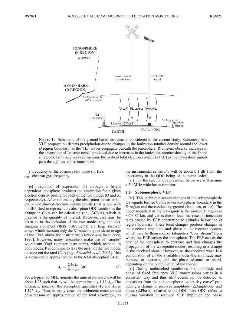
[8] Figure 1 shows a schematic of the ground-basedinstruments we consider in the current study. Subionospheric

radio receivers detect precipitation due to changes in theionization number density around the lower D regionboundary. As VLF waves propagate beneath the ionospherein the Earth-ionosphere waveguide, any change in the heightof the D region boundary will produce changes in thereceived amplitude and phase. Due to the low attenuation ofVLF subionospheric propagation, the EEP-modified iono-spheric region may be far from the transmitter or the receiverand a combination of ionospheric and electromagnetic wavemodeling must be invoked to constrain where the EEP hasmodified the ionosphere. In contrast, riometers observe localEEP-produced changes occurring directly above the instru-ment. In this case the increased ionization number density inthe D and E regions, due to EEP, results in the absorption ofthe HF “cosmic noise” passing through the ionosphere.Finally, the signals arriving at GPS receivers can be used todetermine the total electron content (TEC) as the navigationsignals pass through the entire ionosphere from the satelliteto the receiver. Signals from satellites closest to the groundreceiver can be easily converted to vertical TEC (vTEC)under the assumption of a thin ionosphere, and are thereforeagain a “local” measurement. Generally, vTEC measure-ments are dominated by the ionospheric F region and thechanges which occur in those altitudes [Mendillo, 2006].However, a recent paper has argued that substorm-drivenEEP can lead to significant vTEC changes due to modifica-tion of the ionosphericD and E regions [Watson et al., 2011],leading to the inclusion of this technique in our study.

2.1. Riometers

[9] The riometer utilizes the absorption of cosmic radionoise by the ionosphere [Little and Leinbach, 1959] tomeasure the enhancement of D region electron concen-tration caused by EEP. The riometer technique comparesthe strength of the cosmic radio noise signal received on theground to the normal sidereal variation referred to as theabsorption quiet-day curve (QDC) to produce the change incosmic noise absorption (DCNA). The cosmic radio noisepropagates through the ionosphere and part of the energy isabsorbed due to the collision of the free ionospheric elec-trons with neutral atmospheric atoms. The instantaneousionospheric absorption in decibels is derived from the ratioof the prevailing signal level to this curve [Krishnaswamyet al., 1985]. Typically the absorption peaks near 90 kmaltitude, where the product of electron density and neutralcollision frequency maximizes. Simple expressions for theabsorption of cosmic radio noise (A) can be derived fromthe Appleton-Hartree equations [e.g., Nyland, 2007],

A ¼ 4:61� 10�5

Zh2h1

Ne hð Þ � uen hð Þu2en hð Þ þ 2pf � wBeð Þ2" #

dh dB½ � ð1Þ

whereA absorption (power absorbed on propagation through the

ionosphere) with units of dB;Ne height dependent electron number density profile with

units of electrons per cubic meter;uen dependent effective electron-neutral collision profile

(collisions per second) which can be taken from theempirical fitting of Rodger et al. [1998];

RODGER ET AL.: COMPARISON OF PRECIPITATION MONITORING RS2021RS2021

2 of 13

f frequency of the cosmic radio noise (in Hz);wBe electron gyrofrequency.

[10] Integration of expression (1) through a heightdependent ionosphere produces the absorption for a givenelectron density profile for each of the two modes (O and X,respectively). After subtracting the absorption for an ambi-ent or undisturbed electron density profile (that is one withno EEP flux) to represent the absorption QDC conditions thechange in CNA can be calculated (i.e., DCNA), which inpractice is the quantity of interest. However, care must betaken as to the inclusion of the two modes (AO and AX).Imaging riometers (IRIS instruments) are large receiverarrays which measure only the X-mode but provide an imageof the CNA above the instrument [Detrick and Rosenberg,1990]. However, many researchers make use of “simple”wide-beam Yagi riometer instruments, which respond toboth modes. It is common to take the mean of the two modesto represent the total CNA [e.g., Friedrich et al., 2002]. Thisis a reasonable approximation to the total absorption (AT):

AT ¼ 2AXAO

AX þ AOdB½ � ð2Þ

For a typical 30 MHz riometer the ratio of AX and AO will beabout 1.25 such that AT will be approximately 1.11 AO. Thearithmetic mean of the absorption quantities AX and AO is1.125 AO. Thus, in many cases the arithmetic mean shouldbe a reasonable approximation of the total absorption, as

the instrumental sensitivity will be about 0.1 dB (with theuncertainty in the QDC being of the same order).[11] For the calculations presented below we will assume

a 30 MHz wide-beam riometer.

2.2. Subionospheric VLF

[12] This technique senses changes in the subionosphericwaveguide formed by the lower ionospheric boundary in theD region and the conducting ground (land, sea, or ice). Theupper boundary of the waveguide is the ionized D region at�70–85 km, and varies due to local increases in ionizationrates caused by EEP penetrating to altitudes below the Dregion boundary. These local changes produce changes inthe received amplitude and phase at the receiver system,which may be thousands of kilometers “downstream” fromwhere the EEP strikes the ionosphere. The EEP causes thebase of the ionosphere to decrease and thus changes thepropagation of the waveguide modes, resulting in a changein the received signal. However, as the received wave is acombination of all the available modes the amplitude mayincrease or decrease, and the phase advance or retard,depending on the combination of the modes.[13] During undisturbed conditions the amplitude and

phase of fixed frequency VLF transmissions varies in aconsistent way and thus EEP events can be detected asdeviations from the subionospheric “quiet day curve” pro-ducing a change in received amplitude (DAmplitude) andphase (DPhase), relative to the QDC–here QDC refers todiurnal variation in received VLF amplitude and phase

Figure 1. Schematic of the ground-based instruments considered in the current study. SubionosphericVLF propagation detects precipitation due to changes in the ionization number density around the lowerD region boundary, as the VLF waves propagate beneath the ionosphere. Riometers observe increases inthe absorption of “cosmic noise” produced due to increases in the ionization number density in the D andE regions. GPS receivers can measure the vertical total electron content (vTEC) as the navigation signalspass through the entire ionosphere.

RODGER ET AL.: COMPARISON OF PRECIPITATION MONITORING RS2021RS2021

3 of 13

rather than a CNA. Due to interference between the modesand the strong differences in the D region reflection altitudesbetween day and night, the subionospheric QDC tends tohave a complex form but is highly reproducible [e.g.,Clilverd et al., 1999] albeit with more variation from night tonight than from day to day. For a much more comprehensivereview of this topic we refer the reader to the discussion byBarr et al. [2000] which highlights the development of VLFradio wave propagation measurements particularly over thelast 50 years. Additional discussions on the use of subiono-spheric VLF propagation to sense space weather-producedchanges can be found in the work by Clilverd et al. [2009].Uncertainties in subionospheric VLF QDC will depend uponthe time of day, the receiver design and the backgroundnoise levels. As an example, one EEP-study which reliedupon subionospheric VLF concluded there was a �0.3 dBamplitude uncertainty as a result of removing the subiono-spheric QDC at noon time and a �1 dB amplitude uncer-tainty at nighttime [Rodger et al., 2007].[14] In order to interpret any observed fluctuations in a

received VLF signal it is necessary to reproduce the char-acteristics of the deviations using mathematical descriptionsof VLF wave propagation, and thus determine the ionizationchanges that have occurred around the upper waveguideboundary. In the current study we make use of the U.S. NavyLong Wave Propagation Code (LWPC) [Ferguson andSnyder, 1990] which models VLF signal propagation fromany point on Earth to any other point. The code models thevariation of geophysical parameters along the path as a seriesof horizontally homogeneous segments. To do this, the pro-gram determines the ground conductivity, dielectric constant,orientation of the geomagnetic field with respect to the pathand the solar zenith angle, at small fixed-distance intervalsalong the path. Given electron density profile parameters forthe upper boundary conditions for each section along thepath, LWPC calculates the expected amplitude and phase ofthe VLF signal at the reception point.

2.3. GPS Determined TEC

[15] The absolute total electron content (TEC) can beestimated from the range delay of two radio signals withdifferent frequencies propagating through the low-altitudemagnetosphere and ionosphere between a GPS satellite anda ground station. Absolute TEC is obtained from the pseudo-ranges P1 and P2 for GPS frequencies f1 = 1575.42 MHzand f2 = 1227.60 MHz [Skone, 2001]:

TEC ¼ 1

40:3

1

f 21� 1

f 22

!�1

P1 � P2 � br � bsð Þ; ð3Þ

where br and bs are the receiver and satellite interchannelbias terms, respectively. The uncertainty in absolute TECcan be between 1 and 5 TECu (where 1 TECu = 1016

electrons m�2) due to receiver or satellite biases and mul-tipath effects.[16] Relative changes in TEC can be estimated using the

carrier phase ranges F:

TEC ¼� 1

40:3

1

f 21� 1

f 22

!�1

F1 � F2ð Þ; ð4Þ

assuming that the ambiguities in the signal phase are rela-tively constant in time. These relative variations have muchgreater accuracy, �0.10 TECu [Skone, 2001].[17] The above estimates provide TEC, or relative changes

in TEC, along the entire raypath between satellite to station,and further assumptions must be made to estimate the ver-tical TEC (vTEC) directly upward above the ground station.Typically, the estimated TEC is projected to the local zenithdirection to obtain the vertical TEC using a mapping func-tion M(ɛ) that models the ionosphere as a uniform thin shellwith a well-defined average height h [e.g., Arikan et al.,2003]:

M ɛð Þ ¼ 1� RE cos ɛð ÞRE þ h

� �2" #�1=2

ð5Þ

where RE is the Earth radius, and ɛ is the elevation angleof the satellite measured at the receiver. vTEC can be easilycompared with model predictions since it is the equivalentof the height-integrated electron number density through theionosphere [e.g., Anderson et al., 1987]:

vertical TEC ¼ 10�16

Zh2h1

Ne hð Þ dh TECu½ �: ð6Þ

[18] In this study we will consider the change in vTECwith and without the addition of EEP, which we will defineas DvTEC.

2.4. EEP-Produced Changes in Electron NumberDensity

[19] In order to estimate the response of the variousinstruments to EEP, we start by determining the change inionospheric electron number density over the altitude range40–150 km caused by precipitation. This altitude rangecovers the altitudes of peak energy deposition for electronswith energies from about 1 keV to 10 MeV, which is suffi-cient for our EEP study. The ambient, or undisturbed electrondensity profile, is provided by the International ReferenceIonosphere (IRI-2007) (online from http://omniweb.gsfc.nasa.gov/vitmo/iri_vitmo.html) for the equinox on 21 Marchat 18 UT for “day” conditions and 6 UT for night, with the“STORM” model switched off. As the IRI does not includeall of the D region, particularly during the nighttime, wecombine the IRI results with typicalD region electron densityprofiles determined for high latitudes at noon [Thomsonet al., 2011] and for nighttime conditions [Thomson andMcRae, 2009].[20] For the purposes of the modeling we will first focus

on the location of Island Lake (53.86�N, 265.34�E, L = 5.2),Canada, marked by the yellow square in Figure 2. This sitehosts a NORSTAR riometer and lies close to the midpoint ofthe great circle path from the VLF transmitter NDK (greencircle, North Dakota, 25.2 kHz) and the AARDDVARKVLF receiver at Churchill (58.75�N, 265.1�E, L = 7.6).While we could select any location for our essentially the-oretical comparisons, the point we have chosen provides theadvantage of being applicable to the real world. In latersections, we will use other sites in order to compare directlywith observations during particular events.

RODGER ET AL.: COMPARISON OF PRECIPITATION MONITORING RS2021RS2021

4 of 13

[21] The ionization rate due to precipitating energeticelectrons is calculated by an application of the expressions inthe work by Rees [1989], expanded to higher energies basedon Goldberg et al. [1984]. The background neutral atmo-sphere is calculated using the NRLMSISE-00 neutral atmo-spheric model [Picone et al., 2002]. The equilibriumelectron number density in the lower ionosphere, is provided

by a simplified ionospheric model [Rodger et al., 1998,2007] that has been expanded to encompass a wider rangeof altitudes and ionization rates. The Sodankylä Ion andNeutral Chemistry model (SIC) [Verronen et al., 2005]was run for daytime and nighttime conditions with height-independent, non-varying ionization rates (i.e., ionizationrates that were constant from 40 to 150 km altitude).Empirical weighting factors to the earlier equilibrium elec-tron number density model were determined to best repro-duce the SIC calculations. The results of this are shown inFigure 3 where the solid curves show the electron numberdensity profiles generated by the SIC model, and the dashedcurves are the result of the simplified equilibrium electrondensity model. There is very good agreement between thetwo models for a very wide range of ionization rates over theEEP-relevant altitude range. In practice the ionization rate isnot constant with altitude, and maximizes at an altitudedependent upon the electron energy [Turunen et al., 2009,Figure 3], at least for monoenergetic beam. Note that thesame altitude-constant ionization rate will lead to a largerelectron number density during the day than during the night(although the relative change may well be larger due to thecomparatively weak nighttime ionosphere). Physically, thisis due to photo-detachment of electrons which had attachedto neutral forming a negative ion. During the night this can bea significant loss mechanism for free electrons, but during theday attachment to neutrals is effectively less efficient due tothe competing photo-detachment process.

3. Monoenergetic EEP Beams

[22] In Figure 4 we consider the modeled response of thethree EEP-sensing techniques to monoenergetic electronsprecipitating into the upper atmosphere. While this is not arealistic representation of EEP from the radiation belts orduring substorms, it is instructive as a comparison of therelative sensitivities of the three observation techniques. As

Figure 2. Map showing the location of the modeling point(yellow square), the AARDDVARK receivers at Churchilland Sodankylä (red diamonds) and the VLF transmitterNDK and NAA (green circles). This map also indicates thegreat circle propagation paths between the transmitter andreceiver, as well as a number of fixed L-shell contours eval-uated at 100 km altitude.

Figure 3. Electron number density calculations undertaken for ionization rates (q [electrons m�3]) whichwere constant with altitude for (left) day and (right) night onditions. The solid curves are the results from theSodankylä Ion and Neutral Chemistry (SIC) model, while the dashed curves are from an equilibrium elec-tron density model which has been fitted to the SIC results. Note that the curves for q < 104 electrons m�3,are almost indistinguishable on this plot from the electron number density for q = 0.

RODGER ET AL.: COMPARISON OF PRECIPITATION MONITORING RS2021RS2021

5 of 13

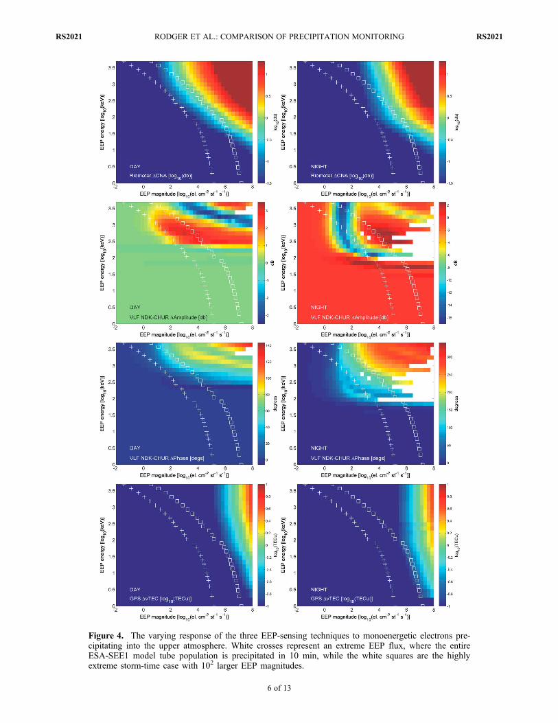
Figure 4. The varying response of the three EEP-sensing techniques to monoenergetic electrons pre-cipitating into the upper atmosphere. White crosses represent an extreme EEP flux, where the entireESA-SEE1 model tube population is precipitated in 10 min, while the white squares are the highlyextreme storm-time case with 102 larger EEP magnitudes.

RODGER ET AL.: COMPARISON OF PRECIPITATION MONITORING RS2021RS2021

6 of 13

noted earlier, we allow for a wide range of EEP energies,spanning from 1 keV to 10 MeV, and take a similarly widerange of precipitation flux magnitudes, from 10�2 electronscm�2 st�1 s�1 to 108 electrons cm�2 st�1 s�1. The upperenergy range is an extreme estimate of precipitation flux forany reasonable radiation belt EEP event, and corresponds tothe approximate flux used to represent 5 keV “auroral”electron precipitation by Turunen et al. [2009, Figure 5]. Inorder to provide bounds for a realistic range of possible EEPflux levels, Figure 4 includes white crosses to show themaximum precipitating flux, calculated by assuming theentire electron flux stored in a L = 5.3 flux tube can beprecipitated out in a 10 min period, calculated using theESA-SEE1 radiation belt model [Vampola, 1997]. Duringstorms the trapped population of the radiation belts can beboosted by several orders of magnitude, and so these higherflux levels are indicated using white squares, representinga very extreme storm time case in which EEP fluxes are100 times larger than the typical flux tube populations pro-vided by the radiation belt model. Note however, thatclearing the entire electron population of a flux tube in10 min should be regarded as a very extreme example ofradiation belt loss.[23] The upper ionosphere electron density profile chan-

ges were calculated as outlined in section 2.4, after whichthe response of each instrument to the ionospheric changewas estimated for a sunlit ionosphere (Figure 4, left) and anighttime ionosphere (Figure 4, right). The first row inFigure 4 presents the calculations of the riometerDCNA, thesecond and third rows present the change in amplitude andphase for the subionospheric VLF propagation case fromNDK to Churchill, and the fourth row presents the GPSderived DvTEC. For the subionospheric VLF propagation,the precipitation is introduced on the section of the greatcircle path which lies from 0.16 to 1.28 Mm from the NDKtransmitter, corresponding to L = 3.5–7, i.e., a reasonablerange for the outer radiation belt. The colorscale has beenlimited to reflect an estimated minimum detectable instru-mental change of �0.05 dB for a riometer and 0.1 TECu forthe GPS vTEC measurement. We have imposed a ceiling of20 dB on the riometer response to reflect an approximatemaximum “real world” value. The maximum modeledDCNA value of�1960 dB is unrealistic. For subionosphericVLF propagation the LWPC calculations fails in some cases,which are shown in white in Figure 4.[24] Figure 4 demonstrates that the three EEP-sensing

techniques have different threshold flux magnitudes andelectron energies that allow the detection of EEP, as well asdifferent responses to day and night ambient conditions. Fortechniques which rely upon electromagnetic radiation pass-ing through the ionosphere, such as riometers and GPS-derived TEC, a sufficiently high EEP flux will eventuallyproduce a detectable response, although for riometers thecontribution of height-varying collision frequency makes theinstrument less sensitive at the highest altitudes consideredhere. In general, riometers are more sensitive to the sameEEP event occurring during the day than during the night,while subionospheric VLF shows the opposite relationship(i.e., more sensitive at night than during day). DvTECchanges are similar during the day and night. For subiono-spheric VLF the minimum detectable EEP energy of�150 keV (day) and �50 keV (night) is controlled by the

differing reflection heights of VLF waves propagating underthe undisturbed ionospheres. In general, the subionosphericVLF technique is more sensitive than the other two techni-ques for EEP with energies over 200 keV, responding to fluxmagnitudes two to three orders of magnitude smaller thandetectable by a riometer. Detectable TEC changes onlyoccur for unrealistically extreme monoenergetic fluxes.[25] Figure 4 emphasizes the complex and nonlinear

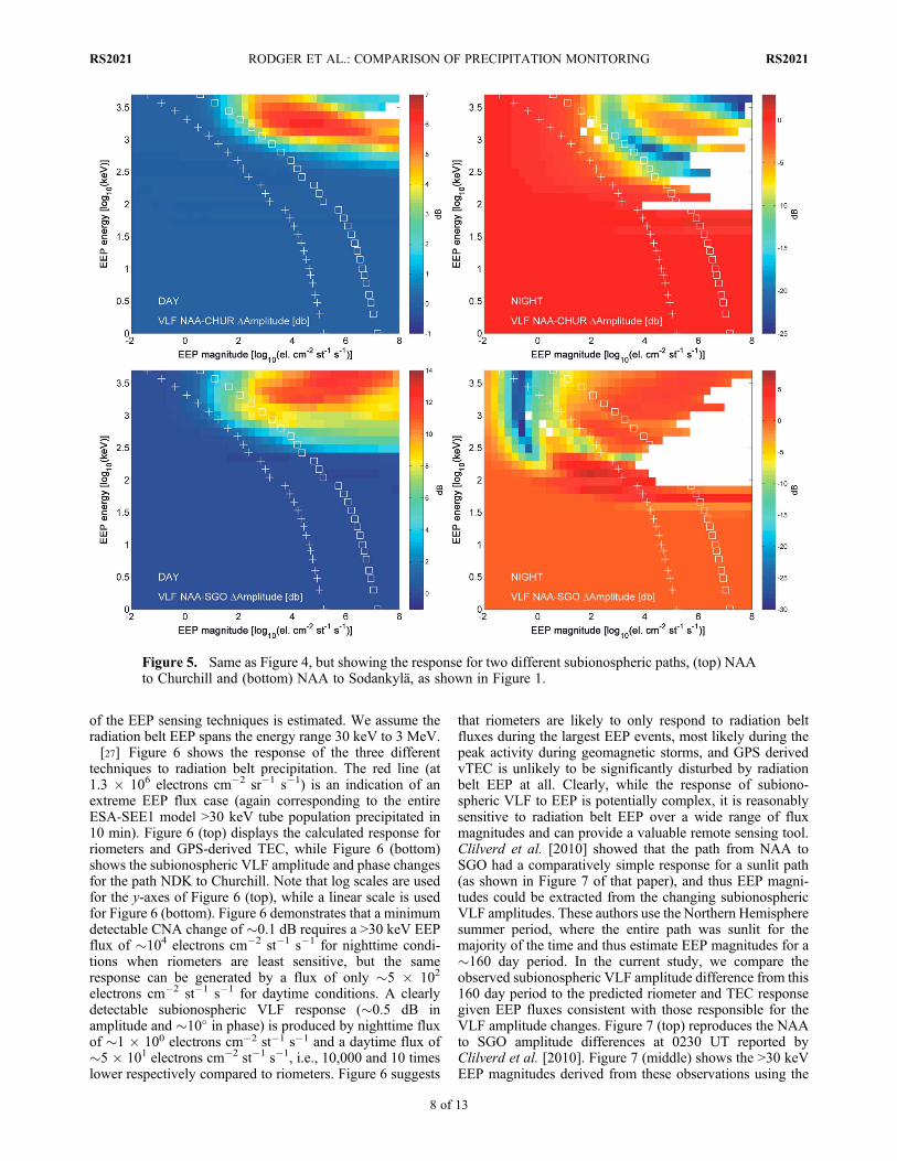
response of subionospheric VLF propagation to an iono-spheric disturbance: both amplitude increases and decreasesseen depending on the energy and flux magnitude of theEEP. Clearly, subionospheric VLF amplitude observationswould be unsuitable for superposed epoch analysis, anapproach which has proved valuable with riometers [e.g.,Longden et al., 2008; A. J. Kavanagh et al., Key features of>30 keV electron precipitation during high speed solar windstreams: A superposed epoch analysis, submitted to Journalof Geophysical Research, 2011]. In contrast, the phasechanges are considerably better behaved with phase advan-ces occurring for most EEP energy and flux conditions.Similar behavior has been reported previously in the sub-ionospheric VLF amplitude and phase response to solarflares [e.g., Thomson et al., 2005]. It is important to note thatthe received VLF broadcast is a summation of multiplemodes after propagation in the Earth-ionosphere waveguide,and so the response of subionospheric VLF amplitude toEEP is highly dependent upon the combination of thetransmitter and the receiver. Figure 5 presents estimates ofamplitude response from two other VLF paths: NAA toChurchill (CHUR; Figure 5, top) and NAA to the SodankyläGeophysical Observatory (SGO; Figure 5, bottom). Thetwo paths are shown in Figure 2. Note that in the latter casewe make use of the daytime ambient ionosphere and thedisturbed ionosphere limits outlined by Clilverd et al.[2010] for consistency with later sections of the currentstudy. Figures 4 and 5 show that the pattern of positive andnegative subionospheric amplitude changes and their mag-nitude is different, even two similar paths (i.e., NDK toChurchill and NAA to Churchill). In addition, the mini-mum flux required for a measureable amplitude deviationvaries strongly from path to path, especially for nighttimeconditions.

4. EEP From the Radiation Belts

[26] As noted above, realistic EEP from the radiation beltsis not well represented by idealized monoenergetic beams.We therefore consider the case of EEP with an energyspectrum provided by experimental measurements fromthe DEMETER spacecraft [Clilverd et al., 2010]. WhileDEMETER primarily measured electrons in the drift losscone, its measurements are more likely to be representative ofthe bounce loss cone than those of the trapped electronfluxes. The typical energy spectra presented by Clilverd et al.[2010] is, however, very similar in form to the energy spectraof the total tube content calculated from the ESA-SEE1radiation belt model (not shown), providing additional con-fidence that this spectra is representative. In the current studywe hold the energy spectrum constant and sweep through arange of EEP flux magnitudes. The model described insection 2 is used to determine the ionization rates and hencethe altered electron density profiles from which the response

RODGER ET AL.: COMPARISON OF PRECIPITATION MONITORING RS2021RS2021

7 of 13

of the EEP sensing techniques is estimated. We assume theradiation belt EEP spans the energy range 30 keV to 3 MeV.[27] Figure 6 shows the response of the three different

techniques to radiation belt precipitation. The red line (at1.3 � 106 electrons cm�2 sr�1 s�1) is an indication of anextreme EEP flux case (again corresponding to the entireESA-SEE1 model >30 keV tube population precipitated in10 min). Figure 6 (top) displays the calculated response forriometers and GPS-derived TEC, while Figure 6 (bottom)shows the subionospheric VLF amplitude and phase changesfor the path NDK to Churchill. Note that log scales are usedfor the y-axes of Figure 6 (top), while a linear scale is usedfor Figure 6 (bottom). Figure 6 demonstrates that a minimumdetectable CNA change of �0.1 dB requires a >30 keV EEPflux of �104 electrons cm�2 st�1 s�1 for nighttime condi-tions when riometers are least sensitive, but the sameresponse can be generated by a flux of only �5 � 102

electrons cm�2 st�1 s�1 for daytime conditions. A clearlydetectable subionospheric VLF response (�0.5 dB inamplitude and �10� in phase) is produced by nighttime fluxof �1 � 100 electrons cm�2 st�1 s�1 and a daytime flux of�5 � 101 electrons cm�2 st�1 s�1, i.e., 10,000 and 10 timeslower respectively compared to riometers. Figure 6 suggests

that riometers are likely to only respond to radiation beltfluxes during the largest EEP events, most likely during thepeak activity during geomagnetic storms, and GPS derivedvTEC is unlikely to be significantly disturbed by radiationbelt EEP at all. Clearly, while the response of subiono-spheric VLF to EEP is potentially complex, it is reasonablysensitive to radiation belt EEP over a wide range of fluxmagnitudes and can provide a valuable remote sensing tool.Clilverd et al. [2010] showed that the path from NAA toSGO had a comparatively simple response for a sunlit path(as shown in Figure 7 of that paper), and thus EEP magni-tudes could be extracted from the changing subionosphericVLF amplitudes. These authors use the Northern Hemispheresummer period, where the entire path was sunlit for themajority of the time and thus estimate EEP magnitudes for a�160 day period. In the current study, we compare theobserved subionospheric VLF amplitude difference from this160 day period to the predicted riometer and TEC responsegiven EEP fluxes consistent with those responsible for theVLF amplitude changes. Figure 7 (top) reproduces the NAAto SGO amplitude differences at 0230 UT reported byClilverd et al. [2010]. Figure 7 (middle) shows the >30 keVEEP magnitudes derived from these observations using the

Figure 5. Same as Figure 4, but showing the response for two different subionospheric paths, (top) NAAto Churchill and (bottom) NAA to Sodankylä, as shown in Figure 1.

RODGER ET AL.: COMPARISON OF PRECIPITATION MONITORING RS2021RS2021

8 of 13

ionospheric model described in section 2.4. Periods wherethe VLF propagation would be influenced by solar protonsimpacting the polar ionosphere have been removed fromFigure 7 (top) and the subsequent calculations. Figure 7(bottom) shows the predicted response in DCNA and DvTECproduced by the estimated EEP fluxes. There is a clearlydetectable change in riometer response during the periods ofpeak EEP fluxes, i.e., during storm times. The right-hand axisof Figure 7 (bottom) clearly demonstrates that there is nochange in vTEC in the presence of stormtime high energyprecipitation above the 0.1 TECu threshold required. It istherefore unlikely that riometers, or GPS-derived TEC can beused to measure radiation belt EEP in “normal” or “small”storm conditions, but that riometers will respond during thelargest precipitation events.

5. EEP From Substorms

[28] Substorms generate EEP when the energy stored inthe Earth’s magnetotail is converted into particle heating andkinetic energy. It has long been recognized that substormsare accompanied by some level of particle precipitationthrough their association with brightening of auroral arcs.

Recent papers have suggested that a very large fractionof the enhanced population energetic electrons (50–1000 keV)observed by geostationary satellites during substorms precip-itate into the atmosphere. Clilverd et al. [2008] concluded thatroughly 50% of the electrons injected near the LANL-97Asatellite during a substorm on 1 March 2006 precipitated inthe region near the satellite, and comparable EEP fluxes werereported by Clilverd et al. [2012] for another THEMISdetected-substorm occurring on 28 May 2010. Both of thesestudies combined the satellite measurements with observationsfrom a riometer and subionospheric VLF instruments. Inaddition, Watson et al. [2011] examined GPS TEC measure-ments during substorms and reported vTEC changes of severalTEC units associated with the substorm. By studying theapparent expansion of the precipitation region due to thesubstorm, they concluded that the bulk of theDvTEC changeoccurred at altitudes of approximately �100 km, i.e., thevTEC was responding to the EEP and not the very con-siderable population of <1 keV electrons that also precip-itate during substorms [Mende et al., 2003]. In order totest this conclusion, we consider the response of riometersand subionospheric VLF during the events examined byClilverd et al. [2008, 2012] and test whether the EEP

Figure 6. The varying response of the three EEP-sensing techniques to EEP with a energy spectrum thatis realistic for precipitation from the radiation belts. (top) The calculated response for riometers and GPS-derived TEC and (bottom) the subionospheric VLF amplitude and phase changes. The red line representsan extreme EEP flux, where the entire ESA-SEE1 model tube population is precipitated in 10 min.

RODGER ET AL.: COMPARISON OF PRECIPITATION MONITORING RS2021RS2021

9 of 13

striking the atmosphere below 150 km can explain thereported vTEC changes.[29] Clilverd et al. [2008, 2012] modeled the substorm

signature in ground-based data using 30 keV–2.5 MeV EEPspectra derived from satellite measurements (LANL-97Aand THEMIS, respectively). In order to model the two sub-storms reported in those papers, we expand the energyspectra to encompass EEP with energies from 1 keV. TheEEP flux at 1 keV is set at 3 � 109 electrons cm�2 st�1 s�1

taken from FAST measurements reported during a substormwhich was said to be “fairly typical” [Mende et al., 2003,Figure 4a]. The flux at 1 keV is joined smoothly using apower law to the 30 keV–2.5 MeV EEP spectra describedabove.[30] Table 1 summarizes the results of this modeling. We

list the observed riometer response at Macquarie Island(54.5�S, 158.9�E, L = 5.4) and the observed subionosphericVLF response at the Australian Antarctic Division stationCasey (66.3�S, 110.5�E, L > 999). We use the signal mea-sured at Casey from the powerful U.S. Navy transmitterNWC, located in western Australia. The first of the twosubstorms occurred on 1 March 2006; the peak riometerDCNA was 2.9 dB, associated with a 15 dB decrease in theamplitude of NWC measured at Casey. We estimate that thisVLF subionospheric amplitude decrease is produced froma >30 keV EEP flux of 2.6 � 107 electrons cm�2 st�1 s�1

[Clilverd et al., 2008] which would lead to a riometerDCNA of 5.4 dB. In contrast, the model suggests that theobserved riometerDCNA of 2.9 dB could be produced froma >30 keV EEP flux of 0.8 � 107 electrons cm�2 st�1 s�1

which would lead to a decrease in the VLF amplitude fromNWC of 9 dB at Casey. The two different predicted EEPspectra for these situations are shown in Figure 8. Case 1 of1 March 2006 represents the predicted spectra from theriometer measurement (DCNA = 2.9 dB, first “CalculationResults” line in Table 1) while Case 2 represents the pre-dicted spectra from the subionospheric VLF measurement(DVLF of �15 dB, second “Calculation Results” line inTable 1) Clearly, there is some uncertainty in the EEPmagnitude, which may come from the high variability ofwinter nighttime amplitudes, but the two EEP fluxes differonly by a factor of three. Both the potential modeling solu-tions lead to significant predictedDvTEC, 3.1 and 4.2 TECu,respectively.[31] The second of the two substorms occurred on 28 May

2010, after the Casey subionospheric VLF receiver wasupgraded such that phase changes could be determined.

Figure 7. A comparison between (top) the variation of theNAA to SGO received amplitudes at 0230 UT in days 100–260 of 2005 (10 April to 17 September 2005), (middle)the >30 keV EEP flux determined from the NAA ampli-tudes, and (bottom) the response of a riometer and a GPSvTEC instrument sensing the same ionospheric disturbanceas the subionospheric VLF instrument. The red line repre-sents an extreme EEP flux, where the entire ESA-SEE1model tube population is precipitated in 10 min. The hori-zontal black line in Figure 7 (bottom) is an indication ofthe lowest riometer detection sensitivity.

Table 1. Summary of Ground-Based EEP Instrument ResponsesDuring Two Substorms Reported by Clilverd et al. [2008, 2012]a

Event DCNA DVLF DvTEC EEP

1 March 2006Observed experimental 2.9 dB �15 dB – –Calculation results 2.9 dB �9 dB 3.1 TECu 0.8 � 107

5.4 dB �15 dB 4.2 TECu 2.6 � 107

28 May 2010Observed experimental 3.2 dB 210� – –Calculation results 3.2 dB 210� 4.8 TUCu 1.1 � 107

aBeneath the experimental observations are the calculated results for themodeling of each of the two events, as described in the text. The EEP valueslisted are >30 keV electron fluxes with units of electrons cm�2 st�1 s�1.

RODGER ET AL.: COMPARISON OF PRECIPITATION MONITORING RS2021RS2021

10 of 13

Clilverd et al. [2012] report a riometer DCNA of 3.2 dB,associated with a 210� phase advance of the signal fromNWC measured at Casey. They argued that the phasechanges should provide a more accurate indication of theEEP because the NWC-Casey quiet day phase variations aremore consistent than the quiet day amplitude variationsduring the nighttime in the winter months. We estimate thatthis VLF subionospheric phase increase is produced froma >30 keV EEP flux of 1.1 � 107 electrons cm�2 st�1 s�1

which leads to a riometer DCNA of 3.2 dB and DvTEC of4.8 TECu. The predicted differential EEP flux for this situ-ation is shown in Figure 8. In this case there is very goodagreement between the EEP flux predicted from both theriometer and the subionospheric phase for this substorm.Our model predicts that an EEP flux of 1.1 � 107 electronscm�2 st�1 s�1 produces DvTEC of 4.8 TECu, which is inthe upper range reported by Watson et al. [2011, Figure 12].[32] The conclusion of Watson et al. [2011] that a signif-

icant fraction of the substorm-associated DvTEC changesoccur in the D and E regions is supported by our calcula-tions. However, we find that only about one-third to one-halfof the DvTEC changes are due to increased ionization ataltitudes below 120 km altitude, with the remainder of thechange due to ionization at higher altitudes.

6. Discussion

[33] While we have shown that the response of subiono-spheric VLF to EEP is complicated, we have also shown thatit is reasonably sensitive to a wide range of flux magnitudesand can provide a valuable remote sensing tool. For anygiven transmitter to receiver great circle path the response ofthe received amplitude to varying EEP conditions can be anincrease or a decrease in amplitude. However, under similarpropagation conditions, the received phase is more likelyto show quasi-linear increases as EEP flux magnitudesincrease. Thus VLF phase measurements are potentially

more useful than amplitude measurements in determiningEEP characteristics. The main caveat associated with thisstatement is associated with time-scales. The VLF phasemeasurement is more difficult to make consistently overlong periods of time in comparison with VLF amplitude.Several factors contribute to this difficulty: phase lockingto unstable transmissions, non-integer broadcast frequen-cies, and the lack of transmitter phase consistency betweentransmitter maintenance cycles or transmitter off-periods.While some VLF transmitters appear to have oscillatorswhich are locked to GPS or atomic clocks and broadcastat the stated frequency, others appear to be offset from thenominal frequency; an example of this is the VLF trans-mitter near Ebino, Japan, which has a nominal operationalfrequency of 22.2 kHz but produces better quality ampli-tude and phase observations if the GPS-locked receiver isset to 22200.1175 Hz. In addition, most operationaltransmitters stop broadcasting once a week for a severalhour period during which maintenance is undertaken,leading to unpredictable leaps in phase. In principle it ispossible to indentify and compensate for many of theseissues, but the longer the period of study the more difficultit is to positively identify phase variations that have beenproduced by EEP. When the perturbations caused by EEPare only minutes or hours long, then VLF phase is a verygood investigative tool. However, if an EEP event lasts formore that a day then phase analysis can become contam-inated by the instrument effects listed above, and greatcare needs to be taken. For events lasting 5–10 days, suchas EEP from the radiation belts, the analysis of VLF phaseis likely to be very difficult. These difficulties could bemitigated if complementary phase information was recordedclose to the transmitters, or if official information about thephase was transmitted.[34] The modeling results presented in section 4 suggest

that, considering the realistic energy spectra and flux range,riometers will only respond to EEP with energies >30 keVduring the largest radiation belt storms, and even thennot particularly strongly. Riometers can respond to EEPevents that include a significant population of electronenergies <30 keV and that includes substorm events. Suchelectrons deposit the majority of their energy above the Dregion (i.e., above �90 km) around the altitude range whereriometer absorption peaks.[35] GPS TEC-measurements are not sensitive enough to

monitor precipitation from the radiation belts, and have onlya small response to substorms. It should be noted, however,that GPS instruments can produce more significant vTECchanges during EEP events if there are a significant popu-lation of electrons with energies <30 keV. For soft EEPevents (5–30 keV) there is only a small variation in riometerCNA, no effect on VLF propagation, but significant changesin vTEC. Watson called this “auroral” precipitation [Watsonet al., 2011].

7. Summary and Conclusions

[36] In order to make best use of the opportunities pro-vided by upcoming space missions such as the RadiationBelt Storm Probes, we have determined the response of threedifferent techniques to different energetic electron precipi-tation (EEP) characteristics. All of the techniques selected

Figure 8. Comparison between the substorm-associateddifferential EEP fluxes for the calculation cases given inTable 1. Case 1 of 01 March 2006 is the first “Calculationresults” line (i.e., 2.9 dB) of Table 1, while Case 2 is forthe second line (5.4 dB).

RODGER ET AL.: COMPARISON OF PRECIPITATION MONITORING RS2021RS2021

11 of 13

have extensive ground-based instrumentation networks andare used to study EEP. Here we focused upon subiono-spheric radiowave propagation measurements (VLF), riom-eter absorption measurements (CNA), and GPS producedtotal electron content (vTEC). All of the three electromag-netic remote sensing techniques are comparatively low cost,as the “transmitter” is either funded independently of thescience goal, as in the case of the subionospheric VLF andGPS satellite networks, or is a natural source, as in the caseof riometers. In our study we contrasted the predicted sen-sitivity and responses of these instruments to idealizedmonoenergetic beams of precipitating electrons, and pre-cipitating spectra derived from in situ experiments whichrepresent energetic electron precipitation from the radiationbelts and during substorms.[37] For the monoenergetic beam case we found that

riometers are more sensitive to the same EEP event occur-ring during the day than during the night, while subiono-spheric VLF showed the opposite relationship. DvTECchanges were similar for both day and night ionosphericconditions. In general, the subionospheric VLF technique ismore sensitive than the other two techniques for EEP withenergies over 200 keV, responding to flux magnitudes twoto three orders of magnitude smaller than that detectable by ariometer. Detectable TEC changes only occurred for extrememonoenergetic fluxes, which appear to be beyond the levelsone expects in reality.[38] For the radiation belt EEP case clearly detectable

subionospheric VLF responses are produced by daytimefluxes that are �10 times lower than required for riometers,while nighttime fluxes can be 10,000 times lower that thatrequired for a riometer viewing the same event, and stillproduce a detectable response in the subionospheric VLFobservations. We found that riometers are likely to onlyrespond to radiation belt fluxes during the largest EEPevents. In contrast, GPS derived vTEC is unlikely to besignificantly disturbed by radiation belt EEP at all. It shouldbe noted that this conclusion refers to EEP with ener-gies >30 keV using an experimentally derived EEP spec-trum; riometers and GPS instruments could produce moresignificant DCNA and vTEC changes during EEP eventsif there were a significant population of electrons withenergies <30 keV.[39] In the case of EEP during substorms, the responses

predicted for the riometer absorption and the subionosphericVLF technique are both significant and clearly detectable.This is also true for the DvTEC, which is at a clearlydetectable level of�3–4 TECu. Half of the vTEC changes insubstorms are due to increased ionization below 120 kmaltitude, which is consistent with the conclusions of a recentstudy [Watson et al., 2011] who speculated that substorm-associated vTEC changes were likely to be occurring in theD and E regions of the ionosphere.

[40] Acknowledgments. C.J.R. would like to thank Lynette Finnie ofDunedin for her support. C.J.R. was supported by the New Zealand MarsdenFund. The research leading to these results has received funding from theEuropean Union Seventh Framework Programme (FP7/2007–2013) undergrant agreement 263218. A.J.K. was supported by the UK Science and Tech-nology Facilities Council (grant ST/G002401/1), C.E.J.W. by the CanadianSpace Agency, and P.T.V. by the Academy of Finland through the project136225/SPOC (Significance of Energetic Electron Precipitation to OddHydrogen, Ozone, and Climate).

ReferencesAlfonsi, L., et al. (2008), Probing the high latitude ionosphere from ground-based observations: The state of current knowledge and capabilitiesduring IPY (2007–2009), J. Atmos. Sol. Terr. Phys., 70(18), 2293–2308,doi:10.1016/j.jastp.2008.06.013.

Anderson, D. N., M. Mendillo, and B. Herniter (1987), A semi-empiricallow-latitude ionospheric model, Radio Sci., 22(2), 292–306, doi:10.1029/RS022i002p00292.

Arikan, F., C. B. Erol, and O. Arikan (2003), Regularized estimationof vertical total electron content from Global Positioning System data,J. Geophys. Res., 108(A12), 1469, doi:10.1029/2002JA009605.

Barr, R., D. L. Jones, and C. J. Rodger (2000), ELF and VLF radio waves,J. Atmos. Sol. Terr. Phys., 62(17–18), 1689–1718, doi:10.1016/S1364-6826(00)00121-8.

Brasseur, G., and S. Solomon (2005), Aeronomy of the Middle Atmosphere,3rd ed., Springer, Dordrecht, Netherlands.

Clilverd, M. A., N. R. Thomson, and C. J. Rodger (1999), Sunrise effects onVLF signals propagated over a long north–south path, Radio Sci., 34(4),939–948, doi:10.1029/1999RS900052.

Clilverd, M. A., C. J. Rodger, and T. Ulich (2006), The importance of atmo-spheric precipitation in storm-time relativistic electron flux drop outs,Geophys. Res. Lett., 33, L01102, doi:10.1029/2005GL024661.

Clilverd, M. A., et al. (2008), Energetic electron precipitation duringsubstorm injection events: High-latitude fluxes and an unexpectedmidlatitude signature, J. Geophys. Res., 113, A10311, doi:10.1029/2008JA013220.

Clilverd, M. A., et al. (2009), Remote sensing space weather events:Antarctic-Arctic Radiation-belt (Dynamic) Deposition-VLF AtmosphericResearch Konsortium network, Space Weather, 7, S04001, doi:10.1029/2008SW000412.

Clilverd, M. A., C. J. Rodger, R. J. Gamble, T. Ulich, T. Raita, A. Seppälä,J. C. Green, N. R. Thomson, J.-A. Sauvaud, and M. Parrot (2010),Ground-based estimates of outer radiation belt energetic electron precip-itation fluxes into the atmosphere, J. Geophys. Res., 115, A12304,doi:10.1029/2010JA015638.

Clilverd, M. A., C. J. Rodger, I. J. Rae, J. B. Brundell, N. R. Thomson,N. Cobbett, P. T. Verronen, and F. W. Menk (2012), Combined THEMISand ground-based observations of a pair of substorm-associated electronprecipitation events, J. Geophys. Res., 117, A02313, doi:10.1029/2011JA016933.

Detrick, D. L., and T. J. Rosenberg (1990), A phased-array radiowaveimager for studies of cosmic noise absorption, Radio Sci., 25, 325–338,doi:10.1029/RS025i004p00325.

Ferguson, J. A., and F. P. Snyder (1990), Computer programs for assess-ment of long wavelength radio communications, version 1.0, Tech.Doc., 1773, Nav. Ocean Syst. Cent., San Diego, Calif.

Friedel, R. H. W., G. D. Reeves, and T. Obara (2002), Relativistic electrondynamics in the inner magnetosphere—A review, J. Atmos. Sol. Terr.Phys., 64(2), 265–282, doi:10.1016/S1364-6826(01)00088-8.

Friedrich, M., M. Harrich, K. Torkar, and P. Stauning (2002), Quantitativemeasurements with wide-beam riometers, J. Atmos. Sol. Terr. Phys., 64,359–365, doi:10.1016/S1364-6826(01)00108-0.

Goldberg, R. A., C. H. Jackman, J. R. Barcus, and F. Søraas (1984), Night-time auroral energy deposition in the middle atmosphere, J. Geophys.Res., 89(A7), 5581–5596, doi:10.1029/JA089iA07p05581.

Green, J. C., T. G. Onsager, T. P. O’Brien, and D. N. Baker (2004), Testingloss mechanisms capable of rapidly depleting relativistic electron flux inthe Earth’s outer radiation belt, J. Geophys. Res., 109, A12211,doi:10.1029/2004JA010579.

Hess, W. N. (1968), The Radiation Belt and Magnetosphere, Blaisdell,London.

Horne, R. B. (2002), The contribution of wave-particle interactions toelectron loss and acceleration in the Earth’s radiation belts during geo-magnetic storms, in The Review of Radio Science, 1999–2002, editedby W. R. Stone, pp. 801–828, IEEE Press, Piscataway, N. J.

Jayachandran, P. T., et al. (2009), Canadian High Arctic Ionospheric Net-work (CHAIN), Radio Sci., 44, RS0A03, doi:10.1029/2008RS004046.

Krishnaswamy, S., D. L. Detrick, and T. J. Rosenberg (1985), The inflec-tion point method of determining riometer quiet day curves, Radio Sci.,20, 123–136, doi:10.1029/RS020i001p00123.

Little, C. G., and H. Leinbach (1959), The riometer—A device for the con-tinuous measurement of ionospheric absorption, Proc. IRE, 47, 315–320,doi:10.1109/JRPROC.1959.287299.

Longden, N., M. H. Denton, and F. Honary (2008), Particle precipitationduring ICME-driven and CIR-driven geomagnetic storms, J. Geophys.Res., 113, A06205, doi:10.1029/2007JA012752.

Lorentzen, K. R., M. D. Looper, and J. B. Blake (2001), Relativistic elec-tron microbursts during the GEM storms, Geophys. Res. Lett., 28(13),2573–2576, doi:10.1029/2001GL012926.

RODGER ET AL.: COMPARISON OF PRECIPITATION MONITORING RS2021RS2021

12 of 13

Mende, S. B., C. W. Carlson, H. U. Frey, L. M. Peticolas, and N. Østgaard(2003), FAST and IMAGE-FUV observations of a substorm onset,J. Geophys. Res., 108(A9), 1344, doi:10.1029/2002JA009787.

Mendillo, M. (2006), Storms in the ionosphere: Patterns and processesfor total electron content, Rev. Geophys., 44, RG4001, doi:10.1029/2005RG000193.

Millan, R. M., and the BARREL Team (2011), Understanding relativ-istic electron losses with BARREL, J. Atmos. Sol. Terr. Phys., 73,1425–1434, doi:10.1016/j.jastp.2011.01.006.

Millan, R. M., and R. M. Thorne (2007), Review of radiation belt relativis-tic electron losses, J. Atmos. Sol. Terr. Phys., 69, 362–377, doi:10.1016/j.jastp.2006.06.019.

Morley, S. K., R. H. W. Friedel, E. L. Spanswick, G. D. Reeves, J. T.Steinberg, J. Koller, T. Cayton, and E. Noveroske (2010), Dropoutsof the outer electron radiation belt in response to solar wind streaminterfaces: Global Positioning System observations, Proc. R. Soc. A,466(2123), 3329–3350, doi:10.1098/rspa.2010.0078.

Newnham, D. A., P. J. Espy, M. A. Clilverd, C. J. Rodger, A. Seppälä,D. J. Maxfield, P. Hartogh, K. Holmén, and R. B. Horne (2011), Directobservations of nitric oxide produced by energetic electron precipitationinto the Antarctic middle atmosphere, Geophys. Res. Lett., 38, L20104,doi:10.1029/2011GL048666.

Nyland, I. (2007), A comparison study between cosmic noise absorptionand flux of precipitating energetic electrons, MSc thesis, Univ. of Bergen,Bergen, Norway.

Picone, J. M., A. E. Hedin, D. P. Drob, and A. C. Aikin (2002),NRLMSISE-00 empirical model of the atmosphere: Statistical com-parisons and scientific issues, J. Geophys. Res., 107(A12), 1468,doi:10.1029/2002JA009430.

Randall, C. E., V. L. Harvey, C. S. Singleton, S. M. Bailey, P. F. Bernath,M. Codrescu, H. Nakajima, and J. M. Russell III (2007), Energetic parti-cle precipitation effects on the Southern Hemisphere stratosphere in1992–2005, J. Geophys. Res., 112, D08308, doi:10.1029/2006JD007696.

Rees,M.H. (1989),Physics andChemistry of theUpper Atmosphere, CambridgeUniv. Press, Cambridge, U. K., doi:10.1017/CBO9780511573118.

Reeves, G. D., K. L. McAdams, R. H. W. Friedel, and T. P. O’Brien (2003),Acceleration and loss of relativistic electrons during geomagnetic storms,Geophys. Res. Lett., 30(10), 1529, doi:10.1029/2002GL016513.

Reeves, G. D., A. Chan, and C. Rodger (2009), New directions for radiationbelt research, Space Weather, 7, S07004, doi:10.1029/2008SW000436.

Rodger, C. J., O. A. Molchanov, and N. R. Thomson (1998), Relaxationof transient ionization in the lower ionosphere, J. Geophys. Res., 103,6969–6975, doi:10.1029/98JA00016.

Rodger, C. J., M. A. Clilverd, N. R. Thomson, R. J. Gamble, A. Seppälä,E. Turunen, N. P. Meredith, M. Parrot, J.-A. Sauvaud, and J.-J. Berthelier(2007), Radiation belt electron precipitation into the atmosphere: Recoveryfrom a geomagnetic storm, J. Geophys. Res., 112, A11307, doi:10.1029/2007JA012383.

Rodger, C. J., M. A. Clilverd, A. Seppälä, N. R. Thomson, R. J. Gamble,M. Parrot, J.-A. Sauvaud, and T. Ulich (2010), Radiation belt electronprecipitation due to geomagnetic storms: Significance to middle atmo-sphere ozone chemistry, J. Geophys. Res., 115, A11320, doi:10.1029/2010JA015599.

Rozanov, E., L. Callis, M. Schlesinger, F. Yang, N. Andronova, andV. Zubov (2005), Atmospheric response to NOy source due to energeticelectron precipitation, Geophys. Res. Lett., 32, L14811, doi:10.1029/2005GL023041.

Seppälä, A., M. A. Clilverd, and C. J. Rodger (2007), NOx enhancements inthe middle atmosphere during 2003–2004 polar winter: Relative signifi-cance of solar proton events and the aurora as a source, J. Geophys.Res., 112, D23303, doi:10.1029/2006JD008326.

Seppälä, A., C. E. Randall, M. A. Clilverd, E. Rozanov, and C. J. Rodger(2009), Geomagnetic activity and polar surface air temperature vari-ability, J. Geophys. Res., 114, A10312, doi:10.1029/2008JA014029.

Skone, S. H. (2001), The impact of magnetic storms on GPS receiverperformance, J. Geod., 75, 457–468, doi:10.1007/s001900100198.

Thomson, N. R., and W. M. McRae (2009), Nighttime ionospheric Dregion: Equatorial and nonequatorial, J. Geophys. Res., 114, A08305,doi:10.1029/2008JA014001.

Thomson, N. R., C. J. Rodger, and M. A. Clilverd (2005), Large solar flaresand their ionospheric D region enhancements, J. Geophys. Res., 110,A06306, doi:10.1029/2005JA011008.

Thomson, N. R., C. J. Rodger, and M. A. Clilverd (2011), Daytime Dregion parameters from long-path VLF phase and amplitude, J. Geophys.Res., 116, A11305, doi:10.1029/2011JA016910.

Thorne, R. M. (2010), Radiation belt dynamics: The importance of wave-particle interactions, Geophys. Res. Lett., 37, L22107, doi:10.1029/2010GL044990.

Turunen, E., P. T. Verronen, A. Seppälä, C. J. Rodger, M. A. Clilverd,J. Tamminen, C.-F. Enell, and T. Ulich (2009), Impact of different ener-gies of precipitating particles on NOx generation in the middle and upperatmosphere during geomagnetic storms, J. Atmos. Sol. Terr. Phys., 71,1176–1189, doi:10.1016/j.jastp.2008.07.005.

Ukhorskiy, A. Y., B. J. Anderson, P. C. Brandt, and N. A. Tsyganenko(2006), Storm time evolution of the outer radiation belt: Transport andlosses, J. Geophys. Res., 111, A11S03, doi:10.1029/2006JA011690.

Vampola, A. L. (1997), Outer zone energetic electron environment update,in Conference on the High Energy Radiation Background in Space,edited by P. H. Solomon, pp. 101–104, NASA Cent. for AeroSpaceInf., Linthicum Heights, Md.

Van Allen, J. A. (1997) Energetic particles in the Earth’s external magneticfield, in Discovery of the Magnetosphere, Hist. Geophys. Ser., vol. 7,edited by C. S. Gillmor and J. R. Spreiter, pp. 235–251, AGU,Washington, D. C., doi:10.1029/HG007p0235.

Van Allen, J. A., and L. A. Frank (1959), Radiation measurements to658,300 km. with Pioneer IV, Nature, 184, 219–224, doi:10.1038/184219a0.

Verronen, P. T., A. Seppälä, M. A. Clilverd, C. J. Rodger, E. Kyrölä,C.-F. Enell, T. Ulich, and E. Turunen (2005), Diurnal variation ofozone depletion during the October–November 2003 solar proton events,J. Geophys. Res., 110, A09S32, doi:10.1029/2004JA010932.

Verronen, P. T., C. J. Rodger, M. A. Clilverd, and S. Wang (2011), Firstevidence of mesospheric hydroxyl response to electron precipitation fromthe radiation belts, J. Geophys. Res., 116, D07307, doi:10.1029/2010JD014965.

Watson, C., P. T. Jayachandran, E. Spanswick, E. F. Donovan, and D. W.Danskin (2011), GPS TEC technique for observation of the evolutionof substorm particle precipitation, J. Geophys. Res., 116, A00I90,doi:10.1029/2010JA015732.

M. A. Clilverd, British Antarctic Survey, National Environment ResearchCouncil, High Cross, Madingley Road, Cambridge CB3 0ET, UK.A. J. Kavanagh, Department of Physics, Lancaster University, Lancaster

LA1 4WA, UK.T. Raita, Sodankylä Geophysical Observatory, University of Oulu,

FI-99600 Sodankylä, Finland.C. J. Rodger, Department of Physics, University of Otago, PO Box 56,

Dunedin 9016, New Zealand. (crodger@physics.otago.ac.nz)P. T. Verronen, Finnish Meteorological Institute, PO Box 503, FI-00101

Helsinki, Finland.C. E. J. Watt, Department of Physics, University of Alberta, Edmonton,

AB T6G 2E1, Canada.

RODGER ET AL.: COMPARISON OF PRECIPITATION MONITORING RS2021RS2021

13 of 13