Continuum mechanicsBefore we can discuss the detailed physics relevant in micro-and nanoscale machines, we need to have an understanding of the mechanical properties of bulk solids.

Continuum mechanics is based on the familiar idea that if we coarse-grain the material, we can effectively understand its gross properties by a small number of well-defined parameters, rather than following each atom.

Hydrogen moleculeN ~ 4Schroedinger eqn.Energy levels

Short carbon nanotubeN ~ 105

Molecular dynamicsNormal modes

Kobe U.l w

h

Continuous solidN ~ 1022

Elasticity theorystresses, strains, normal modes

DefinitionsStresses are forces per unit area.

• Because forces are directed and areas are also directed, stresses are tensorial.

• Usually deal with individual tensorial components (scalars).

l w

hx

z

y

FN

whFN

xx =σ

Normal stress

FS

lwFlwF

Syz

Szy

+=

−=

σ

σ

Shear stresses

First letter indicates direction of surface normal; second indicates direction of force, so

∑=

−3

1jjij dAσ = ith component of force

acting on a surface dA=dA n,

DefinitionsDefine u(r) to be the local displacement of a medium from an undeformed state.

Two points that started out a distance dr apart end up separated by )(' urrr ∇⋅+= ddd

Intuitive idea: stresses result from nonuniform translations.

Looking at one component,

⎟⎟⎠

⎞⎜⎜⎝

⎛

∂

∂−

∂∂

+⎟⎟⎠

⎞⎜⎜⎝

⎛

∂

∂+

∂∂

≡∂∂

i

j

j

i

i

j

j

i

j

i

ru

ru

ru

ru

ru

21

21

uniform rigid rotationstrain tensorlijkφε=ε~≡

Can see from definitions thatVVTr δε =⋅∇= u~

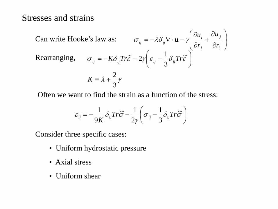
Stresses and strains

Can write Hooke’s law as: ⎟⎟⎠

⎞⎜⎜⎝

⎛

∂

∂+

∂∂

−⋅∇−=i

j

j

iijij r

uru

γλδσ u

Rearranging,

γλ

εδεγεδσ

32

~312~

+≡

⎟⎠⎞

⎜⎝⎛ −−−=

K

TrTrK ijijijij

Often we want to find the strain as a function of the stress:

⎟⎠⎞

⎜⎝⎛ −−−= σδσ

γσδε ~

31

21~

91 TrTrK ijijijij

Consider three specific cases:

• Uniform hydrostatic pressure

• Axial stress

• Uniform shear

Stresses and strains

Uniform pressure p ⎟⎠⎞

⎜⎝⎛ −−−= σδσ

γσδε ~

31

21~

91 TrTrK ijijijij

ijij Kp δε

3−=

No off-diagonal terms: cube remains a cube.

Axial stress σzz = p, all other components zero.

zzzz

zz

KK

pK

εγγσ

γε

⎟⎟⎠

⎞⎜⎜⎝

⎛+

−=

⎟⎟⎠

⎞⎜⎜⎝

⎛+−=

39

31

91

Young’s modulus, E

zzyyxx KK ε

γγεε ⎟⎟⎠

⎞⎜⎜⎝

⎛+−

−==3

2321

Poisson ratio, ν

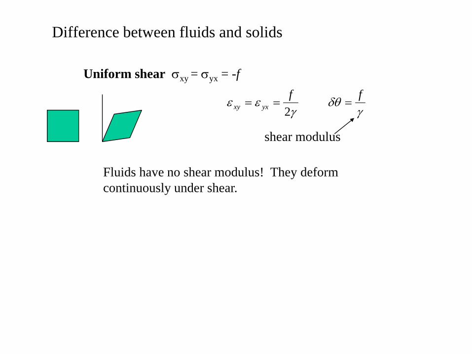
Difference between fluids and solids

Uniform shear σxy = σyx = -f

γεε

2f

yxxy ==γ

δθ f=

shear modulus

Fluids have no shear modulus! They deform continuously under shear.

Numbers and reality

To get some sense of sizes of things:

Stainless steel: E ~ 200 GPa, γ ~ 76 Gpa

Silicon: E ~ 156 GPa, γ ~ 65 Gpa

Silver: E ~ 75 GPa, γ ~ 27 Gpa

All these are assuming linear elasticity. What really happens:

ε

σ

critical yield stressfailurebrittle

ductile

ultimate tensile strength

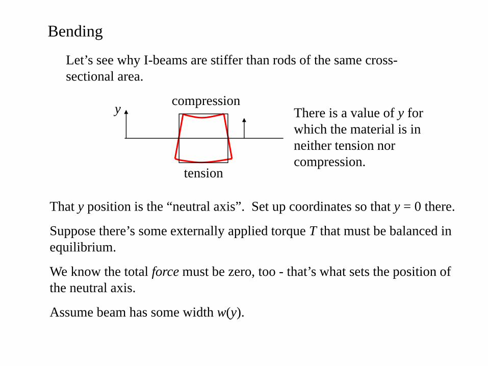
Bending

Let’s see why I-beams are stiffer than rods of the same cross-sectional area.

There is a value of y for which the material is in neither tension nor compression.

y compression

tension

That y position is the “neutral axis”. Set up coordinates so that y = 0 there.

Suppose there’s some externally applied torque T that must be balanced in equilibrium.

We know the total force must be zero, too - that’s what sets the position of the neutral axis.

Assume beam has some width w(y).

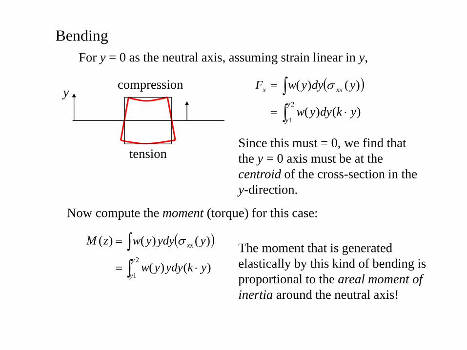
BendingFor y = 0 as the neutral axis, assuming strain linear in y,

y compression

tension

( )

∫∫

⋅=

=2

1)()(

)()(y

y

xxx

ykdyyw

ydyywF σ

Since this must = 0, we find that the y = 0 axis must be at the centroid of the cross-section in the y-direction.

Now compute the moment (torque) for this case:

( )

∫∫

⋅=

=2

1)()(

)()()(y

y

xx

ykydyyw

yydyywzM σ The moment that is generated elastically by this kind of bending is proportional to the areal moment of inertia around the neutral axis!

BendingAgain, for arbitrary coordinates, neutral axis is such that

∫∫=

dyyw

dyyywy

)(

)(

Areal moment of inertia about the neutral axis is then just

∫ −= dyywyyI )()( 2

Examples:

b

h12

3bhI =

radius a

4

4aI π=

I-beams are stiff in flexure because their area is concentrated far from their neutral axis!

Bending δθ/2δθ

Actually computing the shape of the beam,

zyEyzz δδθσ )()( ⋅

=

δz( )

Iz

E

zEyydyyw

yydyywzM

y

y

zz

∂∂

=

⎟⎠⎞

⎜⎝⎛

∂∂

=

=

∫

∫

θ

θ

σ

2

1)(

)()()(

Bigger areal moment of inertia means smaller rate of angular deflection for given bending torque.

Note thatz

uz y

∂

∂≈)(θ

2

2

)()(zu

zEIzM y

∂

∂= Bernoulli-Euler equation

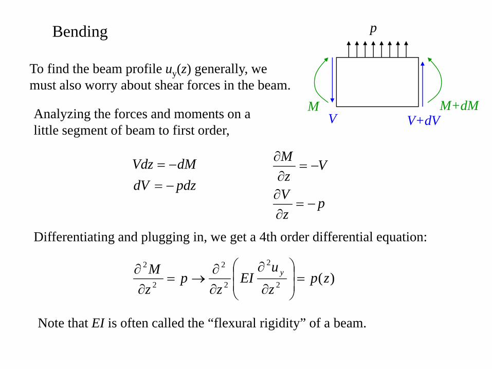
Bending

To find the beam profile uy(z) generally, we must also worry about shear forces in the beam.

p

M M+dMV V+dVAnalyzing the forces and moments on a

little segment of beam to first order,

pdzdVdMVdz

−=−=

pzV

Vz

M

−=∂∂

−=∂∂

Differentiating and plugging in, we get a 4th order differential equation:

)(2

2

2

2

2

2

zpzu

EIz

pzM y =⎟

⎟⎠

⎞⎜⎜⎝

⎛

∂

∂

∂∂

→=∂∂

Note that EI is often called the “flexural rigidity” of a beam.

Boundary conditions and beam shapes For the fixed end of a beam,

0 ,0)0(0

=∂

∂==

=z

yy z

uzu

For a hinged beam,

00)0( ,0)0(0

2

2

=∂

∂→====

=z

yy z

uzMzu

Torsion

An analogous thing happens in torsion.

The shear stress at some position x, y is linearly proportional to its radial position -in a beam with a uniform twist, there is no shear strain on the axis.

The shear stress from that little patch of area contributes an amount of torque proportional to that stress times that radial distance.

Total torque supplied by twisting the beam is proportional to the polar areal moment of inertia:

∫= dAJ 2ρ

For a circular rod of diameter d:32

4dJ π=

For a thin tube of radius a and wall thickness t: taJ 32π=

Torsion

Actually computing the twist of a torsion member:

φ(z) At some radius ρ, the shear strain = zδ

ρδφ

So the contribution to the restoring torque from a patch at that radius is

( )dAz

dAz

2ρφγδρδφγρ

∂∂

=⎟⎠⎞

⎜⎝⎛

Integrating this up, for a given restoring torque T(z),

)()( 2 zJz

dAz

zT∂∂

=∂∂

= ∫φγρφγ

Usual boundary condition for a torsion member is φ(z=0) = 0.

Note that maximum shear stress happens at the outermost radius. For a circular rod of radius a,

JTa

xy =max,σ

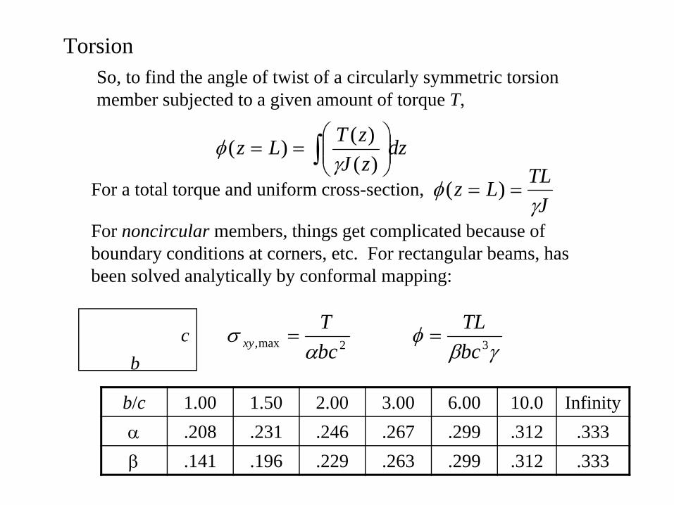
TorsionSo, to find the angle of twist of a circularly symmetric torsion member subjected to a given amount of torque T,

For a total torque and uniform cross-section,

dzzJzTLz ∫ ⎟⎟⎠

⎞⎜⎜⎝

⎛==

)()()(

γφ

JTLLzγ

φ == )(

For noncircular members, things get complicated because of boundary conditions at corners, etc. For rectangular beams, has been solved analytically by conformal mapping:

2max, bcT

xy ασ =c

b γβφ 3bc

TL=

b/c 1.00 1.50 2.00 3.00 6.00 10.0 Infinityα .208 .231 .246 .267 .299 .312 .333β .141 .196 .229 .263 .299 .312 .333

Lagrangian formulationOften we’re interested in the dynamics of a system, not just its statics. Can use Hamiltonian formalism to come up with equations of motion for u(r), the classical deformation field.

Need to be able to write down kinetic and potential energy densities.

Kinetic energy density is simple:

ru 32

21 dKE ∫ ⎟

⎠⎞

⎜⎝⎛= &ρ

Potential energy is a little trickier. Keeping track of the work done when straining a differential volume leads to a conclusion that, in a simple 1d case,

dzz

uEAPE z∫ ⎟

⎟⎠

⎞⎜⎜⎝

⎛⎟⎠⎞

⎜⎝⎛∂∂

=2

21

Longitudinal deformation

dzzu

EIPE y∫ ⎟⎟⎟

⎠

⎞

⎜⎜⎜

⎝

⎛

⎟⎟⎠

⎞⎜⎜⎝

⎛

∂

∂=

2

2

2

21 Lateral deformation (bending)

Lagrangian formulation

To find equations of motion, we can write down the Lagrangian, and do the appropriate variational calculus. For the 1d lateral displacement case, with a driving force on the free end of the beam,

∫ ⎥⎥

⎦

⎤

⎢⎢

⎣

⎡

⎟⎟⎟

⎠

⎞

⎜⎜⎜

⎝

⎛

⎟⎟⎠

⎞⎜⎜⎝

⎛

∂

∂−⎟

⎠⎞

⎜⎝⎛=

Ly

y dzzu

EIuA0

2

2

22

21

21

&ρL

Need to look at variation of time integral of L:

),()(21

212

1

2

1 0

2

2

22 tLutFdz

zu

EIuAdtS y

t

t

Ly

y

t

t

δρδδδ +⎪⎭

⎪⎬⎫

⎪⎩

⎪⎨⎧

⎥⎥

⎦

⎤

⎢⎢

⎣

⎡

⎟⎟⎟

⎠

⎞

⎜⎜⎜

⎝

⎛

⎟⎟⎠

⎞⎜⎜⎝

⎛

∂

∂−⎟

⎠⎞

⎜⎝⎛== ∫ ∫∫ &L

Can do the variations, remembering to play the old games that uy and it’s time derivative can be treated independently, and it’s possible to interchange the orders of differentiation.

Lagrangian formulation

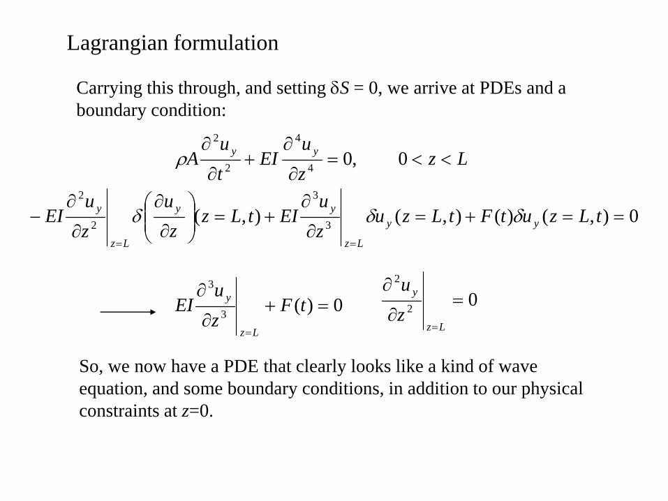
Carrying this through, and setting δS = 0, we arrive at PDEs and a boundary condition:

Lzzu

EItu

A yy <<=∂

∂+

∂

∂0 ,04

4

2

2

ρ

0)(3

3

=+∂

∂

=

tFzu

EILz

y 02

2

=∂

∂

=Lz

y

zu

0),()(),(),( 3

3

2

2

==+=∂

∂+=⎟⎟

⎠

⎞⎜⎜⎝

⎛∂

∂

∂

∂−

==

tLzutFtLzuzu

EItLzz

uzu

EI yy

Lz

yy

Lz

y δδδ

So, we now have a PDE that clearly looks like a kind of wave equation, and some boundary conditions, in addition to our physical constraints at z=0.

Normal modes

Solutions to the fourth-order wave PDE look like mixtures of trig and hyperbolic trig functions tailored to meet the boundary conditions.

General solution for the undriven case:

4/1

4321 )cosh()sinh()cos()sin(),(

⎟⎠⎞

⎜⎝⎛≡

Ω+Ω+Ω+Ω=Ω

EIA

zBzBzBzBzuny

ρα

αααα

This assumes an overall time dependence exp(-iΩt).

Plug this into differential equation, apply appropriate boundary conditions, and solve.

Cantilever case

0

0),0(

0

=∂

∂

=

=z

y

y

zu

tu

0

0

3

3

2

2

=∂

∂

=∂

∂

=

=

Lz

y

Lz

y

zu

zu no moment at free end

no shear force at free end

)cosh()sinh()cos()sin(),( 4321 zkBzkBzkBzkBzu nnnnny +++=Ω

Plugging in z=0 b.c. requires 3142 , BBBB −==

Plugging in z=L b.c. requires 0)sinh()sin(

)cosh()cos(22=

−+

LkLkLkLk

nn

nn

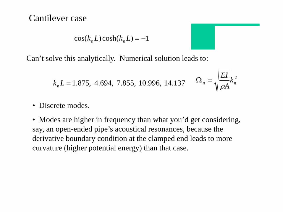
1)cosh()cos( −=LkLk nn

Cantilever case

Can’t solve this analytically. Numerical solution leads to:

1)cosh()cos( −=LkLk nn

14.137 10.996, 7.855, ,694.4 ,875.1=Lkn

2nn k

AEIρ

=Ω

• Discrete modes.

• Modes are higher in frequency than what you’d get considering, say, an open-ended pipe’s acoustical resonances, because the derivative boundary condition at the clamped end leads to more curvature (higher potential energy) than that case.

Doubly-clamped beam

[ ]

2

21

,...132.14 ,996.10 ,853.7 ,730.4 1coshcos

),exp()sinh(sin)cosh(cos),(

nn

nnn

nnnnnnnny

kA

EI

LkLkLk

tizkzkCzkzkCtzu

ρ=Ω

=→=

Ω−−+−=

For the doubly-clamped beam,

0

0),(),0(

0

=∂

∂=

∂

∂

==

== Lz

y

z

y

yy

zu

zu

tLutu

• Frequencies end up being higher than those for, say, an equivalent guitar string because the constraint on the derivative at the clamped ends requires more curvature of the beam.

• Interestingly, same resonance frequencies in the free-free case! Why?

Roukes group, Cal Tech

What about damping?

We recall that the classical damped harmonic oscillator has a velocity-dependent force term in the equation of motion.

Turns out for micromechanical and nanomechanical systems there are different possible damping mechanisms.

Two common ones:

• “Coulomb” damping: damping force proportional to displacement.

This renormalizes the effective spring constant and mass, leading to slightly altered frequencies.

• Usual viscous damping: local damping force proportional to local velocity.

For dissipation, we characterize system by a quality factor Q, defined in the usual way as 2π (total energy in oscillator)/(energy lost per cycle).

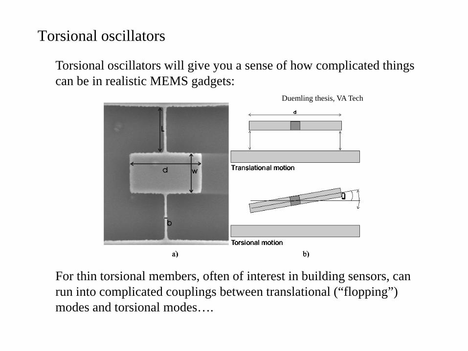
Torsional oscillators

Torsional oscillators will give you a sense of how complicated things can be in realistic MEMS gadgets:

For thin torsional members, often of interest in building sensors, can run into complicated couplings between translational (“flopping”) modes and torsional modes….

Duemling thesis, VA Tech

One key observationNotice that in both torsion and flexure, the maximum strains at a given z are concentrated at the locations farthest away from the neutral axis.

• Dissipative processes that cause damping are typically linear in the energy density at a given position (and so are superlinear in the strain).

• Therefore, surface effects can be extremely important in determining damping, especially in gadgets with large surface-to-volume ratios.

Similarly, the biggest strains for the normal modes typically arise somewhere near the clamping constraint points for a resonator.

• How a resonator is connected to the rest of the world can drastically influence its damping characteristics.

One key observation

An explicit example of this is at right. A finite element calculation has been done for the floppy mode of this torsion paddle, assuming no bending of the paddle for this oscillator.

Color indicated the stress distribution, showing what regions of the structure are contributing the most to damping.

Clearly the clamping points are dominating.

Duemling thesis, VA Tech

Floppy mode

Taking into account mass of paddle, one finds that the lowest floppy mode resonance happens at a frequency like:

ρE

dwLbaf 3

2

2.0≈

Assumes rectangular cross-section for torsional members, ab.

Now to calculate the torsional mode itself….

Torsional mode

Restoring torque is due to the torsional members, which experience maximum twist close to where they join the paddle.

Torsion members must move their own moment of inertia, as well as that of the paddle. Counting only the paddle for a moment,

Resonance frequency ends up being:ργ

π paddleLIabf

3

0 221~

Actual constant of proportionality is a fudge factor ~ 0.3 depending on the aspect ratio of the torsion member cross-section, a/b.

More about damping

Other than simple viscous damping, can run into specific hydrodynamic effects in gases:

• Molecular regime - density of gas is so low that the individual collisions of gas molecules are independent. Does not lead to same damping constant as a gas bulk viscosity would:

wpTk

m

B

2/1

932

⎟⎟⎠

⎞⎜⎜⎝

⎛=Γ

π

Here p is gas pressure and m is mass of gas molecule.

• “Squeeze force” - can get different gas pressure over and under the paddle and torsion members by hydrodynamics.

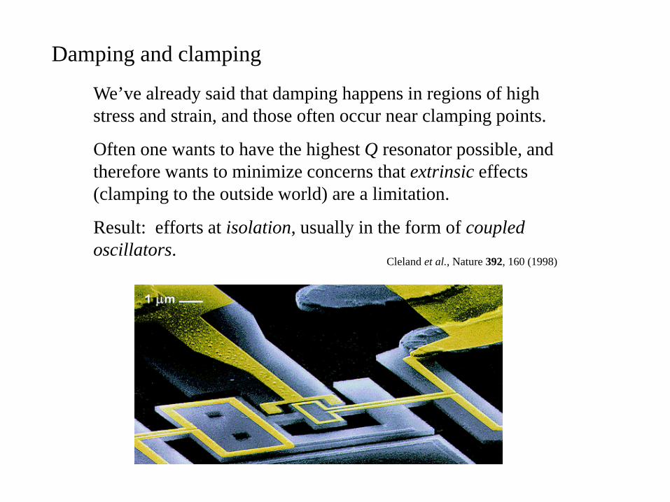
Damping and clamping

We’ve already said that damping happens in regions of high stress and strain, and those often occur near clamping points.

Often one wants to have the highest Q resonator possible, and therefore wants to minimize concerns that extrinsic effects (clamping to the outside world) are a limitation.

Result: efforts at isolation, usually in the form of coupled oscillators.

Cleland et al., Nature 392, 160 (1998)

Size dependence of dampingRoukes, Cal Tech

Similarly, surface effects are of crucial importance, because that’s generally where strains and stresses are maximized.

What is going on at surfaces, and what sets the fundamental limits on the Q that can be achieved in micro- and nano-mechanical resonators?

Localized excitations, quantum effects, etc.

Plasticity

This whole discussion has ignored the atomistic nature of matter. When do we need to worry about these little details?

When we start talking about plastic deformation.

Recall our discussion from the first semester:

It is the propagation of dislocations that lead to plastic deformation.

Remember, it’s much easier to move dislocations than to break all the bonds on an entire crystal plane.

Kittel

Dislocations and plastic deformation

Ductile fracture: smooth propagation of dislocations leading to phenomena like slip:

This leads to “necking”, where under tensile deformation the load-bearing area begins to shrink.

This leads to higher stresses, and correspondingly more strain, until failure.

Dislocations and plastic deformation

• Dislocations carry with them associated elastic fields!

Ex: an edge dislocation is an elastic dipole.

• These elastic fields mean that dislocations interact with each other.

• The result: work-hardening. More and more dislocations in a small volume means dislocations pin each other. Eventually, they cannot propagate. Result: brittle fracture.

Stress concentrations and cracks

The nanoscale structure of matter really does enter into material properties in a direct way that’s still an active area of research: crack initiation and propagation.

Even in continuum limit, deviations in geometry lead to stress concentrations:

Zoom in to a crack in the process of propagating.

At the nm scale, at the crack tip bonds really are being broken. Exactly how does this work?

An active topic of research

Recent results by AFM, for example, show that as cracks propagate in a glass, voids and other defect regions form at the nm scale well in front of the moving crack tip.

Phys. Rev. Lett. 90, 075504 (2003)