1

Basics of continuum mechanics jpb & sms, 2015

BASICS OF CONTINUUM MECHANICS

Continuum mechanics is the mathematical description of deformation and related stresses. The fundamental assumption inscribed in the name is that materials are assumed to be homogeneous, isotropic, continuous and independent of any particular coordinate system. This assumption is based on the intuitive perception that, although nanoscale studies established the discontinuous (atomic, granular, molecular) nature of matter, the macroscopic appearance of solid objects is continuous, i.e. their properties seem to vary gradually, without discontinuity. There are two classical techniques describing the motion of fluids and material points. In Lagrangian formulation the coordinates are glued to and move with a material point through space and time. Therefore, the coordinates of both the material point and the attached variable, such as temperature,

do not change along their trajectory; they are given for a reference time 0t and are time invariant. This formulation has the disadvantage that the reference points move with the flowing fluid. It is therefore difficult to know the state of the fluid at a given point in space and time. In Eulerian formulation one assumes a fixed coordinate system through which material points move as time passes. Therefore, the position of material points and any related quantity changes as a function of time. This change is then described by a partial derivative. A traditional image is a boat going down a river. The Lagrangian description describes the flow as seen from the boat; the Eulerian description describes the flow as seen from a fixed place on the river bank. A less bucolic illustration is to compare a flowing fluid to a car race, one car constituting a particle. Obviously the movement of every car should be defined at any one time to describe the race, i.e. the flow. The initial configuration is the starting line. The Lagrangian approach places a camera on each car to film the race. It is valid if one needs to follow the trajectory of the car that carries the camera; this motion is a function of time since the starting position, but the car looks immobile in the camera; the car velocity is nil, the outside world is in motion. Continuity is expressed by the spatial and temporal continuity between the starting position of the car and its position at the considered instant. The Eulerian approach fixes cameras along the track and records which car passes which camera at which time. Any car has velocity, the outside world is immobile. The velocity of all cars at each instant defines the flow. Continuity is expressed in the differentiability in space and time, at any moment, of physical quantities. Both Lagrangian and Eulerian approaches yield mathematically the same result, but the Eulerian formulation is often found more practical. Describing the motion of a fluid through volume elements at fixed locations (any of the “cameras”) in function of time is termed Eulerian to honour the Swiss mathematician Leonhard Euler (1707-1783) who introduced this type of specification to study fluid motion and the mechanics (dynamics and kinematics) of deforming materials. Considering the object of study as a closed system, the application of continuum mechanics requires respecting three fundamental physical principles:

- Conservation of mass, - Conservation of momentum, both linear and angular, - Conservation of energy.

Conservation means that these three quantities, mass, momentum and energy, cannot change over time, unless an external agent intervenes. Other properties such as density, pressure, temperature, and velocity are assumed to be well-defined at small “material points”, and to vary continuously from point to point. The material point is the geometric center of a small elementary cube large enough to smooth out inter granular “empty” discontinuities but sufficiently small to discount effects of macroscopic changes.

2

Basics in continuum mechanics jpb&sms, 2015

Conservation of mass (continuity equation) This fundamental principle states that the mass of a material object remains constant over time. Mass cannot be added or removed, created or destroyed because the considered continuum is a closed system. The mass of this continuum object is determined by multiplying its volume by its density. The concept of mass conservation is intuitively obvious for rigid-body translation or rotation: The object retains its shape, size, density, and volume. Therefore, the mass of the object remains constant from the initial to the final position and orientation. The same is easily conceived for volume-constant deformation, for example a cube deformed into a same-volume parallelepiped. The shape has changed but the amount of matter, hence mass, is same. Common deformation is a dynamic process that combines the change of shape, displacement and rotation. In this case, consider a cube moving to the right, passing through a vertical gate-in parallel to one cube side. The cube moves without rotation until it entirely goes through another vertical gate-out after which it comes to rest. Since the cube is moving, it takes some time to go through gates –in and –out. The volume can then be defined as:

volume A.v.t=

where A is the elementary area of the cube side, v its velocity and t the time it takes to entirely pass the gates. The mass at gates is density ρ multiplied by volume. At gate-in: ( )in inmass A.v.t− −= ρ

At gate-out: ( )out outmass A.v.t− −= ρ Conservation of mass requires that these two masses are the same and we can eliminate the time dependence by assuming that it is the same at both gates. We obtain:

( )ρ A.v = constant

This equation is largely employed in fluid dynamics. It allows calculating the velocity of flow in a tube. Knowing the velocity at some tube section (area), the conservation of mass tells the velocity for any other tube section. Imagine gate-out is half the size of gate-in (displacement is combined with deformation). Then velocity through gate-out must be twice the velocity at gate-in. The quantity ( )ρ A.v is called mass flow rate.

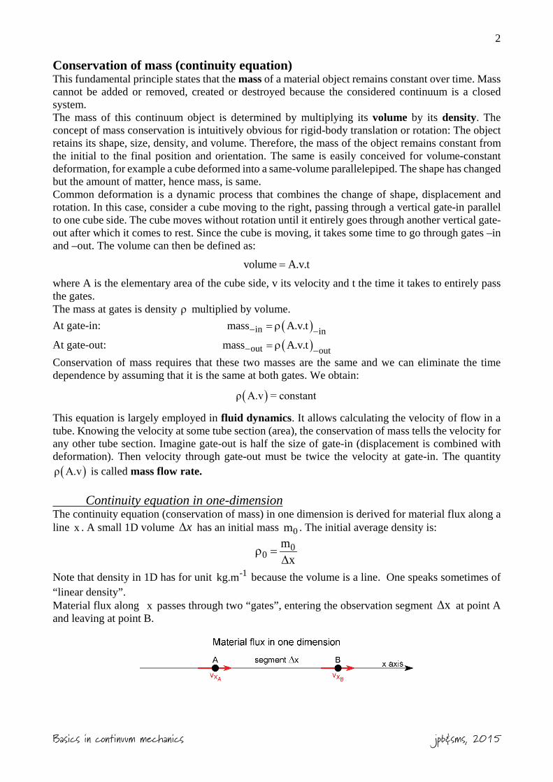
Continuity equation in one-dimension The continuity equation (conservation of mass) in one dimension is derived for material flux along a line x . A small 1D volume x∆ has an initial mass 0m . The initial average density is:

00

mx

ρ =∆

Note that density in 1D has for unit -1kg.m because the volume is a line. One speaks sometimes of “linear density”. Material flux along x passes through two “gates”, entering the observation segment x∆ at point A and leaving at point B.

3

Basics in continuum mechanics jpb&sms, 2015

After an incremental (very small) amount of time t∆ , the mass in x∆ has changed to 1m which is, using the mass fluxes through the boundary points during that time:

1 0 in outm m m m= + − with: in A A A out B B Bv t and v tm m m m= ∆ = ∆= =ρ ρ (1)

where Aρ and Bρ are densities and Av and Bv are the velocities at influx point A and outflux point B, respectively. Thus, the average density 1ρ becomes:

11

mx∆

ρ =

For a very short t∆ the time derivative of the average density is given by the expression:

1 0 1 0m mt t t x t

ρ −ρ −∂ρ ∆ρ≈ = =

∂ ∆ ∆ ∆ ∆

Where t∂ ∂ is the partial derivative symbol meaning rate of change. Using equations (1):

B B A A B B A Av t v t v vt t x x

ρ ∆ −ρ ∆ ρ −ρ∆ρ= − = −

∆ ∆ ∆ ∆

Written in the simpler form:

x( v )t x

∆ ρ∆ρ= −

∆ ∆

or

x( v ) 0t x

∆ ρ∆ρ+ =

∆ ∆

where x B B A A( )v v t v t∆ =ρ ρ ∆ −ρ ∆ is the difference in the mass flux through the two boundary points. If both t∆ and x∆ tend to zero, differences can be replaced by derivatives and equation (2) becomes the 1D continuity equation:

x( v ) 0t x

∂ ρ∂ρ+ =

∂ ∂ (2)

Changing differences (deltas) to derivatives is based on Taylor series, as explained at the end of this lecture. This change is repeated in the following paragraphs.

Continuity equation in two-dimensions The same approach as in 1D can be followed for the two-dimensional case. The observation volume is a small and immobile square with sides of constant lengths, x∆ parallel to the x axis and y∆ parallel to the orthogonal y axis. The initial average density 0ρ calculated from the initial mass 0m is:

00

mx y

ρ =∆ ∆

The 2D density has for unit -2kg.m because the “volume” is area in the plane of observation.

4

Basics in continuum mechanics jpb&sms, 2015

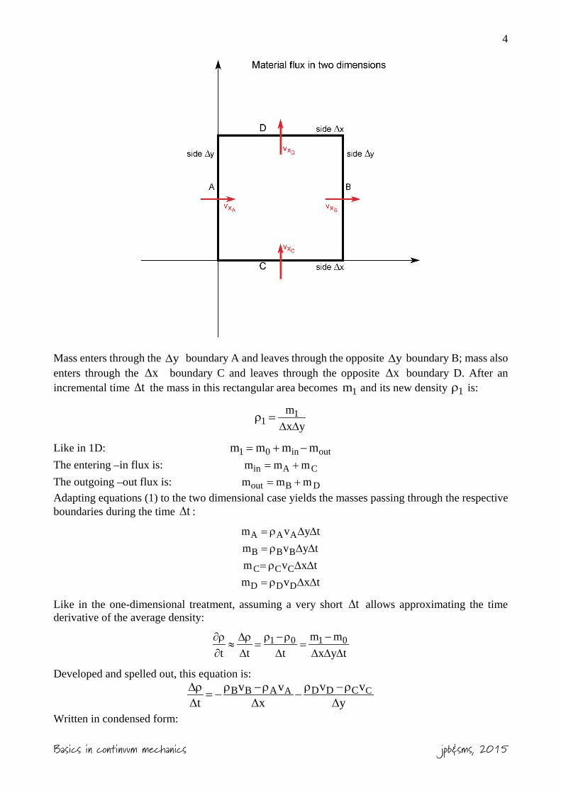
Mass enters through the y∆ boundary A and leaves through the opposite y∆ boundary B; mass also enters through the x∆ boundary C and leaves through the opposite x∆ boundary D. After an incremental time t∆ the mass in this rectangular area becomes 1m and its new density 1ρ is:

11

mx y∆ ∆

ρ =

Like in 1D: 1 0 in outm m m m= + − The entering –in flux is: in A Cm m m= + The outgoing –out flux is: out B Dm m m= + Adapting equations (1) to the two dimensional case yields the masses passing through the respective boundaries during the time t∆ :

A A Am v y t= ρ ∆ ∆

B B Bm v y t= ρ ∆ ∆

C C Cm v x t= ρ ∆ ∆

D D Dm v x t= ρ ∆ ∆

Like in the one-dimensional treatment, assuming a very short t∆ allows approximating the time derivative of the average density:

1 0 1 0m mt t t x y t

ρ −ρ −∂ρ ∆ρ≈ = =

∂ ∆ ∆ ∆ ∆ ∆

Developed and spelled out, this equation is: CA D D CB B A v vv v

t x yρ −ρρ −ρ∆ρ = − −

∆ ∆ ∆

Written in condensed form:

5

Basics in continuum mechanics jpb&sms, 2015

yx ( v )( v )t x y

∆ ρ∆ ρ∆ρ= − −

∆ ∆ ∆

or: yx ( v )( v ) 0t x y

∆ ρ∆ ρ∆ρ+ + =

∆ ∆ ∆

If x∆ , y∆ and t∆ tend all to zero, the derivatives replace differences to formulate the 2D continuity equation:

yx ( v )( v ) 0t x y

∂ ρ∂ ρ∂ρ+ + =

∂ ∂ ∂

Continuity equation in three-dimensions The same reasoning as for the 1D case extended to the 2D consideration can be applied to 3D. In that case, the observation volume is a small, immobile cube with z∆ expressing the third, orthogonal direction. Mass is fluxing in through three orthogonal faces and out through the three orthogonal, opposite faces so that after a short time interval t∆ the density becomes:

11

mx y z∆ ∆ ∆

ρ =

Leading to the approximate expression of the average density in the cube:

1 0 1 0m mt t t x y z t

ρ −ρ −∂ρ ∆ρ≈ = =

∂ ∆ ∆ ∆ ∆ ∆ ∆

Adding expressions of mass, density and velocity through the E-in and F-out z∆ faces to the ABCD faces, equivalent to the A and C -in and B and D –out 2D sides will give:

CA ED D CB B A F F Ev vv v v vt x y z

ρ −ρρ −ρ ρ −ρ∆ρ = − − −∆ ∆ ∆ ∆

Ultimately yielding the continuity equation in 3D:

yx z( v )( v ) ( v ) 0t x y z

∂ ρ∂ ρ ∂ ρ∂ρ+ + + =

∂ ∂ ∂ ∂ (3)

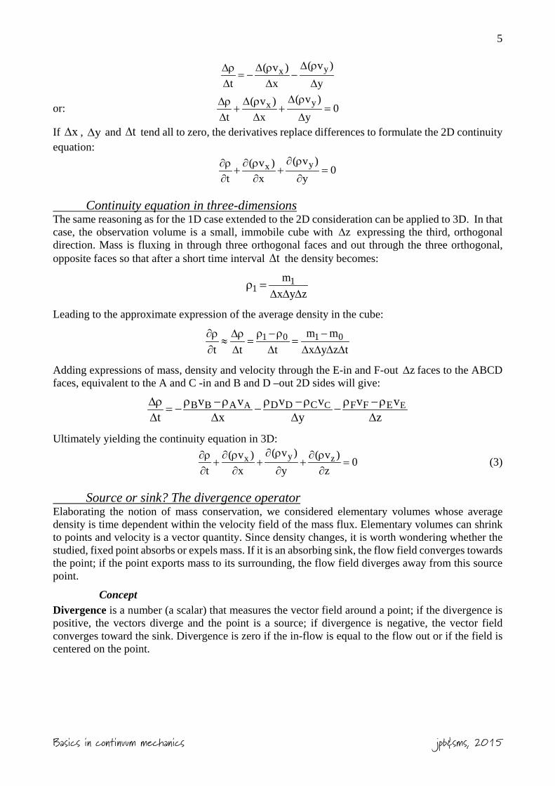
Source or sink? The divergence operator Elaborating the notion of mass conservation, we considered elementary volumes whose average density is time dependent within the velocity field of the mass flux. Elementary volumes can shrink to points and velocity is a vector quantity. Since density changes, it is worth wondering whether the studied, fixed point absorbs or expels mass. If it is an absorbing sink, the flow field converges towards the point; if the point exports mass to its surrounding, the flow field diverges away from this source point.

Concept Divergence is a number (a scalar) that measures the vector field around a point; if the divergence is positive, the vectors diverge and the point is a source; if divergence is negative, the vector field converges toward the sink. Divergence is zero if the in-flow is equal to the flow out or if the field is centered on the point.

6

Basics in continuum mechanics jpb&sms, 2015

Quantifying divergence Divergence denotes how fast the vector field changes (it is a measure of the gradient) in the x, y, and z directions of Cartesian coordinates. Taking xv , yv and zv the velocities parallel to the respective coordinate axes, divergence of the vector field is defined as follows:

In 1D: ( ) xvvx

div ∂=

∂

In 2D: ( ) xyxy

vvvvvx y x y

div∂ ∂ ∂ ∂

= + = ∂ ∂ ∂ ∂

In 3D: ( )x

yx zy

z

vvv vv v

x y z x y zv

div

∂ ∂ ∂ ∂ ∂ ∂= + + = ∂ ∂ ∂ ∂ ∂ ∂

Then we can write the continuity equation (3) as:

( )div v 0t

∂ρ+ ρ =

∂

(4)

Note that this expression is valid for 1D, 2D and 3D, as long as one deals with a continuously differentiable vector field. Note also that it is important for the definition of the scalar product that the left vector is a row vector while the right vector is a column vector.

Symbolizing divergence The right side of the equations for 2D and 3D indicates that the divergence of the velocity field can be expressed mathematically by the scalar product of a vector containing only the difference operators with another vector containing the components of the velocity vector. Divergence is represented by an up-side down delta, ∇ called Nabla (also Del operator). This symbol is a fictional vector of partial derivatives x∂ ∂ with respect to x, y∂ ∂ with respect to y, z∂ ∂ with respect to z:

7

Basics in continuum mechanics jpb&sms, 2015

x y z ∂ ∂ ∂

∇ = ∂ ∂ ∂

Plugging i

, j

and z the three standard unit vectors of the Cartesian coordinate system, it is:

In two dimensions: i jx y∂ ∂

∇ = +∂ ∂

In three dimensions: i j zx y z∂ ∂ ∂

∇ = + +∂ ∂ ∂

Writing only .v∇

is obviously handier than expressing the three components: yx zvv v.v

x y z∂∂ ∂

∇ = + +∂ ∂ ∂

Incompressibility In many situations relevant to geological problems, volume, pressure and temperature variations are negligible. Therefore, geomaterials have a constant density:

0t

∂ρ=

∂

Thus, equation (4) is reduced to:

( )div v 0ρ =

Since density is constant, it can be taken in front of the divergence operator. The entire equation (left and right sides) can be divided by density, which therefore disappears from the above equation. The assumption of constant density hence assumption results in the incompressible continuity equation:

yx zv 0vv v.

x y z=

∂∂ ∂∇ = + +∂ ∂ ∂

(5)

This equation is commonly employed in geodynamic modeling, although it is often a weighty simplification.

Conservation of momentum (force balance) Displacement results from a net force that acts on any object. This net force includes various external and internal forces. The linear momentum is a vector quantity expressing the force or energy of a moving body to keep moving in the same direction unless another new force deviates it, or slows it down or stops it. The linear momentum p of a moving body or particle is due to its mass and its motion. It is therefore a constant equal to the product of its mass m and velocity v :

p m.v=

Momentum takes the forms of linear momentum and angular momentum L , which is the product of the body's or particle’s moment of inertia I (i.e., a measure of its resistance to changes in its rotation velocity) and its angular velocity ω .

L I.= ω

The total momentum of a closed system is equal to the combination and the sum of linear momenta and angular momenta of all particles. This total momentum keeps a constant value unless some new outside force (including torque) is applied on the studied, closed system of several, possibly interacting objects. The total momentum will change also if there is exchange of matter with the outside of the system. The SI unit of momentum is kilograms meters/second (kg m.s-1).

8

Basics in continuum mechanics jpb&sms, 2015

Relation to force Newton’s second law of motion stating that force = mass times acceleration can be written as the change of momentum/time. If a constant force F is applied for a time interval t∆ , the momentum of the object on which this force is applied changes as:

p F t∆ = ∆

In differential form, the rate of change in momentum (or impulse) is equal to the force acting on it:

p vF m m.at t

∂ ∂= = =∂ ∂

(6)

where a is acceleration and applying the already introduced principle of mass conservation (i.e. mass is constant with time). This is the second Newton's law of motion. Expressed qualitatively, momentum of an object is a constant; it is neither created nor destroyed; it is only changed through the action of external forces and with interaction with other objects. Importantly, it is always the total momentum that is conserved.

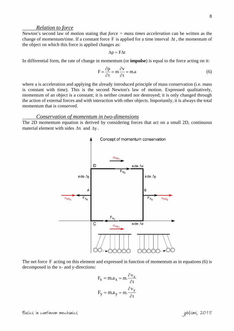
Conservation of momentum in two-dimensions The 2D momentum equation is derived by considering forces that act on a small 2D, continuous material element with sides x∆ and y∆ .

The net force F acting on this element and expressed in function of momentum as in equations (6) is decomposed in the x- and y-directions:

xx x

vF m.t

m.a ∂=

∂=

yy y

vm.

tF m.a

∂=

∂=

9

Basics in continuum mechanics jpb&sms, 2015

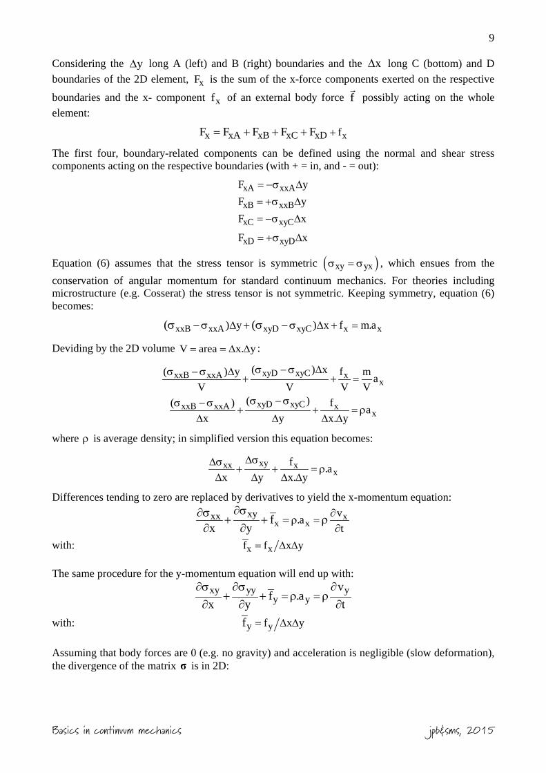
Considering the y∆ long A (left) and B (right) boundaries and the x∆ long C (bottom) and D boundaries of the 2D element, xF is the sum of the x-force components exerted on the respective

boundaries and the x- component xf of an external body force f

possibly acting on the whole element:

xx xA xB xC xD fF F F F F += + + +

The first four, boundary-related components can be defined using the normal and shear stress components acting on the respective boundaries (with + = in, and - = out):

xA xxA

xB xxB

xC xyC

xD xyD

F yF yF x

F x

= −σ ∆= +σ ∆= −σ ∆

= +σ ∆

Equation (6) assumes that the stress tensor is symmetric ( )xy yxσ = σ , which ensues from the conservation of angular momentum for standard continuum mechanics. For theories including microstructure (e.g. Cosserat) the stress tensor is not symmetric. Keeping symmetry, equation (6) becomes:

xxB xxA xyD xyC x x) y ) x f m.a( (−σ ∆ + −σ ∆ + =σ σ

Deviding by the 2D volume V area x. y= = ∆ ∆ :

xyD xyCxxB xxA xx

( ) x( ) y f m aV V V V

σ −σ ∆σ −σ ∆+ + =

xyD xyCxxB xxA xx

( )( ) f ax y x. y

σ −σσ −σ+ + = ρ

∆ ∆ ∆ ∆

where ρ is average density; in simplified version this equation becomes:

xyxx xx

f .ax y x. y

∆σ∆σ+ + = ρ

∆ ∆ ∆ ∆

Differences tending to zero are replaced by derivatives to yield the x-momentum equation:

xx x

xyxx v.at

fx y

∂ρ =

∂

∂σ∂σ + + = ρ∂ ∂

with: x xf f x y= ∆ ∆ The same procedure for the y-momentum equation will end up with:

xy yy yy y

vf .a

x y t∂σ ∂σ ∂

+ + = ρ = ρ∂ ∂ ∂

with: yy f x yf = ∆ ∆

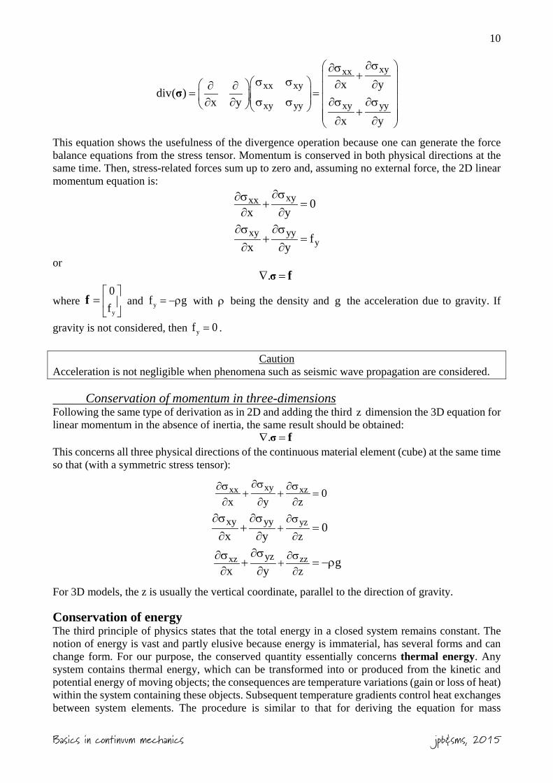
Assuming that body forces are 0 (e.g. no gravity) and acceleration is negligible (slow deformation), the divergence of the matrix σ is in 2D:

10

Basics in continuum mechanics jpb&sms, 2015

xyxxxx xy

xy yy xy yy

x ydiv( )

x yx y

∂σ ∂σ+ σ σ ∂ ∂ ∂ ∂ = = σ σ ∂σ ∂σ∂ ∂ + ∂ ∂

σ

This equation shows the usefulness of the divergence operation because one can generate the force balance equations from the stress tensor. Momentum is conserved in both physical directions at the same time. Then, stress-related forces sum up to zero and, assuming no external force, the 2D linear momentum equation is:

y

xyxx

xy yy

0x y

fx y

∂σ∂σ + =∂ ∂∂σ ∂σ

+ =∂ ∂

or .σ f∇ =

where y

0f

=f and yf g= −ρ with ρ being the density and g the acceleration due to gravity. If

gravity is not considered, then yf 0= .

Caution Acceleration is not negligible when phenomena such as seismic wave propagation are considered.

Conservation of momentum in three-dimensions Following the same type of derivation as in 2D and adding the third z dimension the 3D equation for linear momentum in the absence of inertia, the same result should be obtained: .∇ =σ f This concerns all three physical directions of the continuous material element (cube) at the same time so that (with a symmetric stress tensor):

xyxx xz

yz

xz zz

xy yy

yz

0x y z

z

z

0x y

gx y

∂σ∂σ ∂σ+ + =

∂ ∂ ∂∂σ

+∂

∂σ+

∂

∂σ ∂σ+ =

∂ ∂∂σ∂σ + = −ρ

∂ ∂

For 3D models, the z is usually the vertical coordinate, parallel to the direction of gravity.

Conservation of energy The third principle of physics states that the total energy in a closed system remains constant. The notion of energy is vast and partly elusive because energy is immaterial, has several forms and can change form. For our purpose, the conserved quantity essentially concerns thermal energy. Any system contains thermal energy, which can be transformed into or produced from the kinetic and potential energy of moving objects; the consequences are temperature variations (gain or loss of heat) within the system containing these objects. Subsequent temperature gradients control heat exchanges between system elements. The procedure is similar to that for deriving the equation for mass

11

Basics in continuum mechanics jpb&sms, 2015

conservation. The easy to perceive 1D temperature equation introduces to the 2D and 3D equations to reach the heat equation, which describes the temperature distribution in an object as a function of space and time.

Heat Equations Heat conduction in one dimension

Heat conduction describes the transfer of thermal energy from hot domains or atoms to neighbouring, colder domains or atoms. In 1D heat can only flow along a conductive x-axis , which possesses several physical properties specified by a set of quantities. For thermal problems, those are: - Specific heat (x)c , which is the amount of heat energy needed to raise (or /decrease) one unit of

mass of the material by one degree in temperature. This property is described by difference operators in the following equation:

xQ m c T∆ = ∆ (7) where Q∆ is the amount of heat supplied/substracted (in J), m is the mass, xc is the heat capacity at constant pressure (in J/(kg. K) or J/(kg.°C)) and T∆ is the change in temperature. Possible variations of (x)c along the axis may be ignored as a first approximation.

- Mass density (x)ρ , the mass per unit volume of material, is expressed in kg/m3 (or g/cm3). This quantity also may vary along the axis.

The time dependence is represented by three fundamental functions: - Thermal conductivity (x)k (in W/(m.K) or W/(m.°C)), a measure of the ability of the material to

conduct heat from a hot to a cold region. In 1D, this can be treated as a constant, as a first approximation.

- Heat flux: (x,t)ϕ characterizes the amount of thermal energy that flows through a point per unit time (expressed in Watt = J/s/m2). Hence, it represents the rate at which heat energy is transferred along the x-axis, positive in one direction (usually from left to right), negative in the opposite direction.

- Heat energy generated or absorbed at a small volume per unit time: (x,t)Q represents any external source or sink. It is positive if heat energy is added to the system at that region and time, negative if heat energy is removed from the system at that point and time. Like for mass conservation, energy must flow in or out of a “control volume” (in 1D volume = segment) or energy must be produced or destroyed within this volume if energy changes with time.

The Lagrangian procedure has been detailed for the conservation of mass in 1D. Defining the temperature T at any point x and time t as a space and time function: (x,t)T , the 1D heat equation is in differential form:

( )(x) (x) x,tdTc Qdt x

∂ϕρ = − +

∂ (8)

which is for temperature equivalent to equation (2) for mass. All terms in equation (8) have units of power (J/s) per unit volume. This equation presents two unknown functions, energy c. .Tρ and flux ϕ . The heat flux ϕ is eliminated by applying the Fourier’s law of thermal conduction, which states that the amount of heat q passing through a point is equal to the product of the thermal conductivity of the material and the negative local temperature gradient. In differential form:

12

Basics in continuum mechanics jpb&sms, 2015

( ) ( )x,t xTkx∂

ϕ = −∂

(9)

Implementing equation (9) into equation (8) gives:

( ) ( )(x) (x) x x,tdT Tc k Qdt x x

∂ ∂ ρ = + ∂ ∂ (10)

The three physical properties (x)c , (x)ρ and (x)k are here treated as constant in a uniform material but they may depend on temperature; this assumption simplifies equation (10) to:

( )2

x,t2dT Tc. k Qdt x

∂ρ = +

∂

Dividing both sides by the constant c.ρ :

( )2 x,t2

QdT k Tdt c. c.x

∂= +

ρ ρ∂ (11)

where k c.ρ is the thermal diffusivity K (units are m2/s). This equation is further reduced if there is no external source or sink ( )x,tQ 0= .

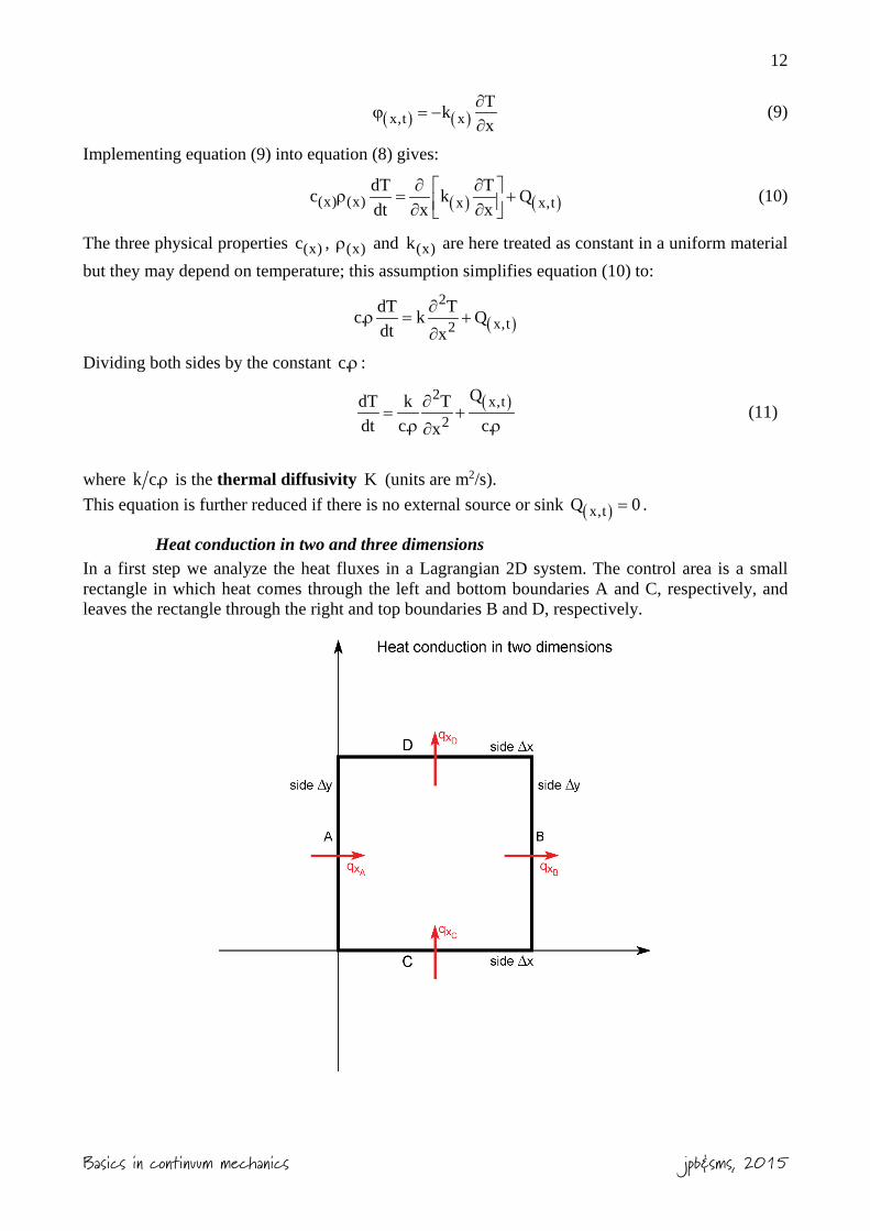
Heat conduction in two and three dimensions In a first step we analyze the heat fluxes in a Lagrangian 2D system. The control area is a small rectangle in which heat comes through the left and bottom boundaries A and C, respectively, and leaves the rectangle through the right and top boundaries B and D, respectively.

13

Basics in continuum mechanics jpb&sms, 2015

Equation (9) applies for each heat flux component through the boundaries of the rectangle delimiting the control area. The amount of energy q passing through each side is:

A

B

C

D

A x

B x

C y

D y

Q q y t

Q q y t

Q q y t

Q q y t

∆ = ∆ ∆

∆ = ∆ ∆

∆ = ∆ ∆

∆ = ∆ ∆

And the heat flux through the area is: A B C DQ Q Q Q Q∆ = ∆ −∆ + ∆ −∆

If there is an internal heat source intQ∆ within the Lagrangian area, the total heat flux becomes. A B C D intQ Q Q Q Q Q∆ = ∆ −∆ + ∆ −∆ + ∆

The change in temperature due to the heat that comes in and leaves the rectangle is described by equation (7). Therefore:

i A B C D intm c T Q Q Q Q Q∆ = ∆ −∆ + ∆ −∆ + ∆ substituting:

A B C Di x x y y intm c T q y t q y t q x t q x t Q∆ = ∆ ∆ − ∆ ∆ + ∆ ∆ − ∆ ∆ + ∆ arranged to:

( ) ( )B A D Ci x x y y intm c T q q y t q q x t Q∆ = − − ∆ ∆ − − ∆ ∆ + ∆ Which can be divided by t∆ and V x y= ∆ ∆ :

( ) ( )D CB A y yx x inti

q q x tq q y tm T QcV t x y t x y t V t

− ∆ ∆− ∆ ∆∆ ∆= − − +

∆ ∆ ∆ ∆ ∆ ∆ ∆ ∆

becomes in simplified form: ( ) ( )D CB A y yx x int

iq qq qm T Qc

V t x y V t−−∆ ∆

= − − +∆ ∆ ∆ ∆

in which m V is per definition density ; simplifying intQ Q V t= ∆ ∆ and taking the limiting case where all ∆ tend to zero yields the differential expression:

yxi

qdT qc Qdt x y

∂∂ρ = − − +

∂ ∂

Using equation (10) yields:

( ) ( )i x ydT T Tc k k Qdt x x y y

∂ ∂ ∂ ∂ ρ = + + ∂ ∂ ∂ ∂

Which has only one unknown, temperature T (which is a scalar, not a vector as velocity). Q may be a function of time and space variables. Expanding equation (10) to 3D (and omitting the third direction for 2D) writes as:

( )2 2 2 x,t2 2 2

QdT k T T Tdt c. c.x y z

∂ ∂ ∂= + + + ρ ρ∂ ∂ ∂

(12)

where: Q can be a function of time and space variables. ( )t,x,y,zT T= is temperature as a function of time and space.

T t∂ ∂ is the rate of temperature change at a point;

14

Basics in continuum mechanics jpb&sms, 2015

2 2T x∂ ∂ , 2 2T y∂ ∂ and 2 2T z∂ ∂ are the second spatial derivatives (thermal conductions) of temperature in the x, y, and z directions, respectively;

Exercise – manipulation Write it with del operator

( )x,t2 QdT k Tdt c. c.

= ∇ +ρ ρ

Internal heat generation Function (11) represents temperature of a body that obeys the heat equation. This body may generate heat per unit volume at a rate given by the function ( )x,tQ , which includes a source varying in space

and time. This is the case for highly radiogenic rocks in which the decay of radioactive isotopes produces heat. Exothermic metamorphic reactions can be another internal source of heat.

Viscous dissipation - shear heating Surface forces are doing work on a deforming body and the power input (J/s) is proportional to the product of force times velocity (N.m/s=J/s). A part of this power input, or rate of deformation energy, is irreversibly dissipated as heat. This power input can be mathematically transformed into the product of stress times velocity gradient, and this product has units of power per unit volume. The power per unit volume can in turn be transformed into heat and is often termed heat production Hshear due to shear forces that depends on both the magnitude of the deviatoric stress tensor and the strain rate tensor. Hshear is defined as:

y yx xshear xx yx xy yy

v vv vH = σ +σ +σ +σx y x y

∂ ∂∂ ∂∂ ∂ ∂ ∂

where ijσ are the components of the deviatoric stress tensor and iv are the velocities in the corresponding Cartesian directions. The dissipation function governs the rate at which mechanical energy is converted to heat during viscous flow.

Radiogenic heat production Radioactive heat (measured in Wm-3) is the main internal heat source of the Earth. The increment of radiogenic heat ( )rE∂ produced in a small cylinder of rock of section a and length x∂ over an increment of time t∂ is:

A.a. x. t A. V. t∂ ∂ = ∂ ∂ with A the depth-independent rate of radiogenic heat production.

Heat conservation The 2D Energy conservation is described by the heat equation with the heat conduction advection, the heat source and the heat production due to shear heating (all terms have units of power per unit volume):

y yx xx y xx yx yy

v vdT T T v vc k k Qdt x x y y x y x y

∂ ∂ ∂ ∂ ∂ ∂ ∂ ∂ ρ = + + + σ +σ + +σ ∂ ∂ ∂ ∂ ∂ ∂ ∂ ∂ (13)

In which the first frame is heat conduction-advection, Q the heat source and the right frame the heat production due to shear heating.

15

Basics in continuum mechanics jpb&sms, 2015

Heat advection Heat can also be transported by motion. Heat advection is the replacement of a volume at temperature T1 with an equivalent volume at temperature T2. In Eulerian description, heat advection (transport of the boat from one place to the next) must be calculated. The time derivative of temperature, /dT dt , is called material time derivative because temperature is a function of position and time. Since coordinates are a function of time, that is x = x(t), expanding the total time derivative with the chain rule of differentiation for the 1D case yields:

( )( )x

dT t,x t T T x T x T T T= + = + = +vdt t x t t t x t x

∂ ∂ ∂ ∂∂ ∂ ∂

∂ ∂ ∂ ∂∂ ∂ ∂ ∂∂

For a Lagrangian formulation dT/dt corresponds to T t∂ ∂ (partial derivative) while for an Eulerian formulation dT/dt corresponds to the partial derivative plus the velocity terms, as shown in equation (13). The advection term is the scalar product of velocity times temperature gradient in the direction of the velocity. In 3D:

x y zdT T T T Tv v vdt t x y z

∂ ∂ ∂ ∂= + + +∂ ∂ ∂ ∂

(14)

where / t∂ ∂ and / , ,x y z∂ ∂ are partial derivatives assuming that all other variables (except that of the derivative) are constant (compare equation 13 with equation 3 obtained for mass conservation, where the variable is density).

Constitutive equations and closed system of equations Conservation equations, which are material independent, cannot be solved without additional information. For example, the two force balance equations, one for mass and one for energy, are four equations in 2D. However, there are six unknowns: two velocities, three stress tensor components and temperature. Thus the four conservation equations are underdetermined; additional equations on the deformation behavior of the studied material (see lecture on rheology-lithospheric strength profiles) allow solving the continuum mechanical problem. The material-dependent, constitutive equations relate stresses to velocities (for fluids) or displacements (for solids). In 2-D, for fluids, the total stresses ( )xx yy xy, ,σ σ σ are separated into a

mean stress ( )( )xx yy 2σ +σ and deviatoric stresses ( )xx yy xy, ,τ τ τ , which are the deviation from

the mean stress.: ( )

( )

yxxxx xx

xxyy

xy xy

y

yyyy

σ στ = σ -

2σ σ

τ =2

τ

+-σ

= σ

+

The deviatoric stress are independent of the mean stress and can be formed entirely from shear components. From the two top of the above three equations follows: xx yyτ = −τ .

Exercise Derive the relation xx yyτ = −τ

Pressure P is often defined as the negative of mean stress:

16

Basics in continuum mechanics jpb&sms, 2015

( )x yx yP / 2σ σ+= −

Pressure, or the mean stress, is an independent quantity that has to be calculated. For compressible fluid, pressure controls the volumetric deformation (dilatation). In tensorial form the total stresses are then:

xx xy xx xy

xy xy yyy y

P 0= - +

0

σ σ τ τ

σ σ τ τP

The deviatoric stresses control the change in shape (shearing) and are related to the spatial gradients of the velocity (i.e. strain rates) by the viscosity, η . For incompressible fluids, the total stresses are:

xxx

y

yxx

y

y

y

vPx

vP

yvv

y x

σ +2

σ +2

σ

∂= − η

∂∂

= − η∂

∂ ∂= η + ∂ ∂

(15)

In 2D, two force balance equations, one mass conservation equation, one energy conservation equation and three constitutive equations (14) make a closed system of seven equations for the seven unknowns x y xx yy xyv , v , , , , P and Tτ τ τ . In 3D, three force balance equations, one mass conservation equation, one energy conservation equation (all equations are given above for 3D), and six constitutive equations represent a closed system of eleven equations for the eleven unknowns

x y z xx yy zz xy xz yzv , v , v , , , , , , , P and Tτ τ τ τ τ τ .

Exercise Write down the six constitutive equations for 3D in normal form and in tensorial form.

Reducing the number of equations for the 2D case We now only consider the 2D situation because for 2D the two force balance equations and the mass conservation equation can be combined into a single equation. As stated in the previous few lines for 2D fluids, the closed system of equations consists of seven equations (four conservation equations and three constitutive equations) for seven unknowns (two velocities, three stresses, pressure and temperature). For example, assuming incompressible flow (equation 5 in 2D) without gravity ( )yf 0= , constant thermal parameters (in equation 12) and substituting the constitutive equations (equation 14) into the force balance equations yields:

yx x

y yx

vv vy x

v vvy

P 0x x y x

force balanceP 0

x y y yx

∂ ∂η η + ∂ ∂

∂ ∂η +

∂ ∂ ∂ ∂ + − = ∂ ∂ ∂ ∂

∂ ∂ ∂ ∂ + − = ∂ ∂ ∂ ∂ η

∂ ∂

2

2

yx vv 0 mass conservation

x y∂∂

+ =∂ ∂

17

Basics in continuum mechanics jpb&sms, 2015

222 2 y yx x

2i

2

2v vdT k T T v v energy conservation

dt c x y x yx y

∂ η η η ∂ ∂ ∂ ∂ ∂ = + + + + + ρ ∂ ∂ ∂ ∂ ∂ ∂

2 2

These four equations include four unknowns (two velocities ( x yv and v ), the pressure P and the temperature T). The two force balance equations consider a variable viscosity, which is essential, for example, for folding or necking. When viscosity is assumed constant, it can be moved in front of the spatial derivatives. In addition, the mass conservation equation can be modified by either taking the derivative with respect to y on both sides or taking the derivative with respect to x on both sides:

yx

2yx

2

2 yx2

vvx y

vvy x y

vvx yx

∂∂= −

∂ ∂

∂∂ ∂= −

∂ ∂ ∂

∂∂ ∂− =

∂ ∂∂

(16)

These relations can be used to eliminate the cross-derivatives yx vv and

y x x y∂∂ ∂ ∂

∂ ∂ ∂ ∂

from the force balance equation. By applying relations (15) one applies automatically the incompressibility condition. Using equations (15), the force balance relation becomes:

2x x

2

2y

2

2

2y

2

2

v vy

v v

x

P 0xx

P 0yy

∂η + ∂ ∂ η

∂ ∂

+

− =∂∂

∂ ∂−

∂ ∂∂ =

These two equations are two force balance equations for constant viscosities. They are now again underdetermined because they include the three unknowns x yv , v and P . One can take the derivative with respect to y of the x-balance equation and the derivative with respect to x of the y-balance equation. By doing this, both equations include the same term:

P Pory x x y∂ ∂ ∂ ∂∂ ∂ ∂ ∂

Substracting both equations eliminates the terms with the pressure and one obtains a single force balance equation for two velocities. The two unknown velocities can be represented by the derivatives of a so-called stream function, ϕ

x

y

y

vx

v ∂ϕ= −

∂∂ϕ

=∂

Substituting the stream function derivative for the velocities into the single force balance equation yields

18

Basics in continuum mechanics jpb&sms, 2015

4 4 4

4 2 2 42 0x x y yϕ ϕ ϕ∂ ∂ ∂+ + =

∂ ∂ ∂ ∂

The above equation is the so-called biharmonic equation (one equation for one unknown ϕ ). Using tensorial operatores the biharmonic equations can be written as

4 20 or 0∇ ϕ = ∆ ϕ = where the Laplace operator

( )( )2

2 2

2 2

div grad

x y

∆ϕ = ∇ ϕ = ∇⋅∇ϕ = ϕ

∂ ϕ ∂ ϕ∆ϕ = +

∂ ∂

The biharmonic equation is essential for and is the basis for most of the analytical solutions in fluid dynamics. One should be aware that solutions of the biharmonic equations are only valid for fluids with a constant viscosity. A biharmonic equation exists only for 2D flow or for 3D spherical and cylindrical flow (i.e. 3D flows with only two spatial derivatives, e.g. with respect to one angle and the radius).

Exercises: Derive the stream function equation from the two force balance equations with constant viscosity Show that the stream function x yϕ = ⋅ ⋅ε fulfills the mass conservation equation, the force balance and that it represents pure shear.

Approximations using Taylor series Taylor series are infinite sums of values. These values are calculated from the derivatives at all points of a smooth function. By this means, one predicts what the function looks like near a considered point. This procedure consists in subdividing a smooth, complicated function, hence its representative curve, into a suite of small segments. The average slope of any segment is the approximate slope of the curve (function) between the two end points. Derivatives reduce infinitesimally small segments to a point and yield the “rate of change” of this slope at any point. Then the sum of derivative values describes well the function. The advantage is to reduce complicated functions to basic arithmetic (addition, subtraction, multiplication, division). The first, second, third (and so on up to nth) derivatives of the studied function ( )f x and substituting the value of a are needed to get a close approximation to the function in the neighborhood of the number x a= . Then these values have to be multiplied by corresponding powers of ( )x a− to obtain

the Taylor Series expansion of the function ( )f x about x a= :

( ) ( ) ( ) ( ) ( )2 3 42 3 4f (a) f (a) f (a) f (a)f x f (a) x a x a x a x a ...

1 2 3 4∂ ∂ ∂ ∂

≈ + − + − + − + − +! ! ! !

This infinite sum can be written in the more convenient, compact sigma notation as

( ) ( )n n

n 0f (a)f x x an!

∞=

∂≈ −∑

19

Basics in continuum mechanics jpb&sms, 2015

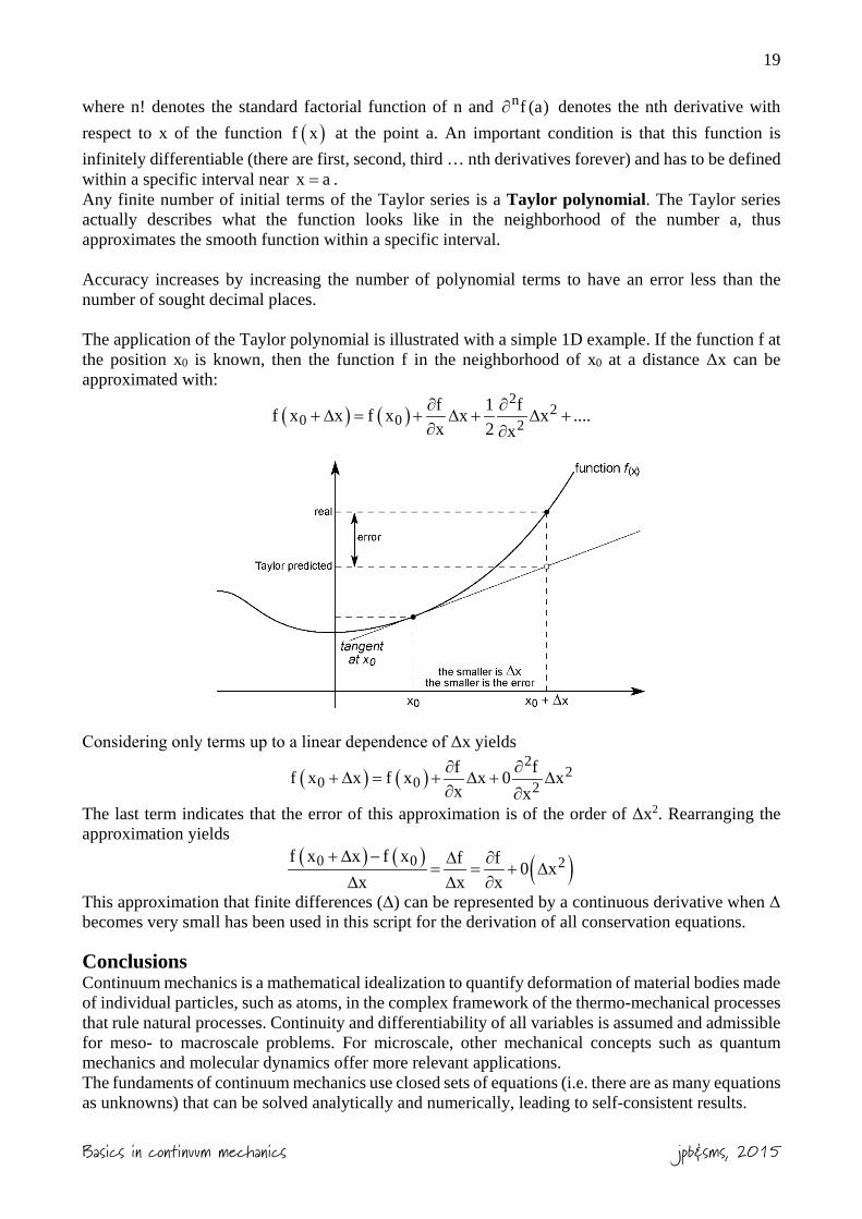
where n! denotes the standard factorial function of n and nf (a)∂ denotes the nth derivative with respect to x of the function ( )f x at the point a. An important condition is that this function is infinitely differentiable (there are first, second, third … nth derivatives forever) and has to be defined within a specific interval near x a= . Any finite number of initial terms of the Taylor series is a Taylor polynomial. The Taylor series actually describes what the function looks like in the neighborhood of the number a, thus approximates the smooth function within a specific interval. Accuracy increases by increasing the number of polynomial terms to have an error less than the number of sought decimal places. The application of the Taylor polynomial is illustrated with a simple 1D example. If the function f at the position x0 is known, then the function f in the neighborhood of x0 at a distance Δx can be approximated with:

( ) ( )2

20 0 2

f 1 ff x x f x x x ....x 2 x∂ ∂

+ ∆ = + ∆ + ∆ +∂ ∂

Considering only terms up to a linear dependence of Δx yields

( ) ( )2

20 0 2

f ff x x f x x 0 xx x∂ ∂

+ ∆ = + ∆ + ∆∂ ∂

The last term indicates that the error of this approximation is of the order of Δx2. Rearranging the approximation yields

( ) ( ) ( )0 0 2f x x f x f f 0 xx x x

+ ∆ − ∆ ∂= = + ∆

∆ ∆ ∂

This approximation that finite differences (Δ) can be represented by a continuous derivative when Δ becomes very small has been used in this script for the derivation of all conservation equations.

Conclusions Continuum mechanics is a mathematical idealization to quantify deformation of material bodies made of individual particles, such as atoms, in the complex framework of the thermo-mechanical processes that rule natural processes. Continuity and differentiability of all variables is assumed and admissible for meso- to macroscale problems. For microscale, other mechanical concepts such as quantum mechanics and molecular dynamics offer more relevant applications. The fundaments of continuum mechanics use closed sets of equations (i.e. there are as many equations as unknowns) that can be solved analytically and numerically, leading to self-consistent results.

20

Basics in continuum mechanics jpb&sms, 2015

One set includes the conservation equations for mass, linear and angular momentum and energy. These equations are material-independent. Another set includes the constitutive equations that describe the deformation behavior (rheology) of particular materials, including rocks for geological applications. These equations are material dependent and are experimentally determined. Continuous functions, differential and integral calculus are the tools to describe the bulk deformation, setting aside minute details of the studied bodies. In any case, one should keep aware that every solution is valid only for specific initial and boundary conditions.

Recommended literature Batchelor G.K. - 1967. An introduction to fluid mechanics.Cambridge University Press, Cambridge,

615 p.

Fowler C.M.R. - 1990. The solid Earth.Cambridge University Press, Cambridge, 472 p.

Gerya T.V. - 2010. Introduction to numerical geodynamic modelling.Cambridge University Press, Cambridge, 345 p.

Malvern L.E. - 1969. Introduction to the mechanics of a continuous medium, Prentice-Hall series in engineering of the physical sciences, Englewood Cliffs, New Jersey, 713 p.

Mase G.T. & Mase G.E. - 1999. Continuum mechanics for engineers, Boca Raton : CRC, 377 p.

Turcotte D.L. & Schubert G. - 2002. Geodynamics, Second Edition ed.Cambridge University Press, Cambridge, 456 p.