Continuously Variable Transmission Cvt 120531120859 Phpapp02
Abstract—From the perspective of vehicle driving, the
relationship between driveline efficiency and fuel efficiency is a
trade-off. Moreover, there are differences in each driver’s
preference in the ranges of driveline and fuel efficiency. For
these reasons, the optimization between driveline efficiency and
fuel efficiency is applied by considering personal driving
characteristics. A study using a continuously variable
transmission (CVT) control algorithm has advantages because
continuous gears have a lot of freedom for control. Therefore,
the target probability, which is related to the driving
characteristics, is applied to the CVT gear shifting control
algorithm based on a CVT vehicle model and verified.
Index Terms—Controller, CVT, driveline efficiency,
economy mode, fuel efficiency, modeling, personal driving
characteristic, sporty mode.
I. INTRODUCTION
From the perspective of powertrain system development,
increases in driveline and fuel efficiency are the most
important factors to satisfy intensified low pollution
restrictions and the demands of customers [1]-[3]. In the
powertrain research field, there are efforts to increase the
driveline and fuel efficiency. Power management system
(PMS) technology, an integration control technique for
engine and transmission, provides a dramatic improvement
of driveline and fuel efficiency through the control of engine
speed and torque. In the study of PMS technology, the
driver’s driving characteristics are considered predominant
factors in developing a control algorithm for the
transmission-shifting ratio.
The problem is that there is a trade-off relationship
between driveline efficiency and fuel efficiency regarding the
control of the transmission-shifting ratio [4]. To optimize this
relationship, a specific standard should be devised. However,
it is difficult to select an optimum value that exactly fits the
driving characteristics of all drivers. Before such a selection
can be predicted, a transmission control algorithm that can
apply driving characteristics should be developed based on a
vehicular model.
To develop the transmission control algorithm, adaptive
transmission control (ATC) is generally considered to reflect
the driving characteristics. To develop an ATC, an evaluation
of the driving characteristics, driving conditions, and
environmental decisions are seriously considered indexes of
Manuscript received September 28, 2018; revised April 1, 2019. The authors are with the Korea Automotive Technology Institute, 31214
Chungnam, Republic of Korea (e-mail: [email protected]).
the driving characteristics. However, such a scoring is not
objective and the ATC standards can easily be changed when
the target vehicle is changed because it also changes the
driving characteristics. Therefore, a more exact and universal
(generally applicable) control algorithm should be developed
using a probability control algorithm.
In this study, a probability control algorithm is devised to
increase the universality of a target probability. This is a
proportion between driving with optimized driveline
efficiency (sporty mode) and with optimized fuel efficiency
(economy mode) that is used to apply the driving
characteristics. The probability control algorithm, which is
related to the shifting ratio control algorithm, was developed
based on a continuously variable transmission (CVT) vehicle
model that allows a designer to control the effect of
optimization on driveline and fuel efficiency.
In Section II of this paper, the development of a CVT
vehicular model based on a powertrain model and a vehicle
and road loads model is described to verify the control logic
in the simulation environment. In Section III, the target
probability tracking controller (probability control algorithm),
which allows the vehicle to reflect the driver’s driving
characteristics, is described.
II. VEHICULAR MODEL BASED ON A VEHICLE TEST
To study the control algorithm, a vehicular model was
developed. The model comprises the powertrain model and
vehicle and road load model because the major consideration
is longitudinal dynamics [5]. An automatic transmission (AT)
vehicular model was developed using dynamic formulas
derived from the application of commercialized AT vehicle
test results. Based on the AT vehicular model, a new CVT
vehicular model was developed and verified.
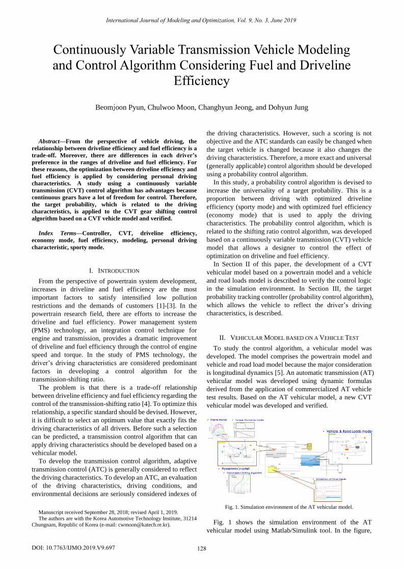
Fig. 1. Simulation environment of the AT vehicular model.
Fig. 1 shows the simulation environment of the AT
vehicular model using Matlab/Simulink tool. In the figure,
Continuously Variable Transmission Vehicle Modeling
and Control Algorithm Considering Fuel and Driveline
Efficiency
Beomjoon Pyun, Chulwoo Moon, Changhyun Jeong, and Dohyun Jung
International Journal of Modeling and Optimization, Vol. 9, No. 3, June 2019
128DOI: 10.7763/IJMO.2019.V9.697

the top left block in the simulation environment is the
powertrain model, which includes the engine map, torque
converter model, and transmission-shifting algorithm based
on the test results [6]. The right block in the simulation
environment is the vehicle and road load model, which
includes the surroundings and vehicle information. The
formulas of the two models are as follows [7].
2[ ( )x w w tf e t wF I N I I = − − +
2 ] /tf e f d wN T N I r+ −
(1)
( ) sinx xf xr A xf xr
Wa F F D R R W
g= + − − + −
(2)
where e tf wN = ,
eI is the engine inertia [kgm2]; e is the
angular acceleration of the engine (rad/s); eT is the engine
torque (Nm); tI is the transmission inertia (kgm2);
dI is the
differential gear inertia (kgm2); fN is the gear ratio of
differential gear (-); wI is the wheel inertia (kgm2);
w is the
angular acceleration of the wheel (rad/s); r is the wheel
effective radius (m); and xF is the traction force (N). Here,
xF is the traction force (N); xR is the rolling resistance (N);
AD is the drag force (N); xa is the vehicle acceleration
(m/s2); is the road slope (rad); W is the weight of the
vehicle (kg); and g is the acceleration of gravity (m/s2).
Formula (1) describes the powertrain dynamics. In this
formula, the engine power is transferred to the drive wheels.
Formula (2) describes the vehicle and road load dynamics.
The formula shows how the power from the powertrain
dynamics is used to calculate the actual acceleration of the
vehicle. Therefore, in Fig. 1, the AT vehicular model using
these formulas is described, and the specifications of an
actual commercial vehicle are applied to the model. The
specifications of the commercialized vehicle are as follows.
TABLE I: SPECIFICATIONS OF A COMMERCIAL VEHICLE
Table I shows the parameters of the vehicular model that
describes the actual commercialized vehicle. As shown in Fig.
1, the parameters were applied to the model using the
Matlab/Simulink tool.
To verify a longitudinal vehicle model, its maximum error
and correlation of longitudinal speed are generally compared.
Therefore, by comparing the vehicle test results, the
vehicular model was verified using the output (the maximum
error and correlation of the longitudinal speed) with the same
input of throttle position corresponding to the accelerator
position sensor.
(a)
(b)
Fig. 2. AT vehicular model verification.
As shown in Fig. 2(a), the same input of throttle position,
which was used in the vehicle test, is used in the simulation.
From this condition, the graph shows that the longitudinal
speed of the test result and that of the vehicular model
simulation are similar. To show the quantitative results, the
maximum error and correlation were used, and the
correlation formula used is as follows.
1
2 2
1 1
( )( )
( ) ( )
n
k k
k
n n
k k
k k
x x y y
r
x x y y
=
= =
− −
=
− −
, (3)
where, 1 1
,n n
k k
k k
x yx y
n n= =
= =
Formula (3) is Pearson’s product-moment coefficient of
correlation (Pearson’s r) [8]. In this formula, the r-square
value is the correlation value. On the basis of these results,
the AT vehicular model was developed with a maximum
error of 2.93 km/h and correlation of 99.68%.
International Journal of Modeling and Optimization, Vol. 9, No. 3, June 2019
129

Fig. 3. Advantages of a CVT.
As shown in Fig. 3, a CVT can continuously change the
gear ratio without shifting shock and shifting loss. Hence,
CVT is more controllable than AT, and this makes it useful
for taking an optimal value of driveline or fuel efficiency.
The CVT vehicular model was developed based on the
previously developed AT vehicular model, and the shifting
schedule was created using the AT shifting schedule. Then,
the CVT vehicular model was verified by comparing it with
the AT vehicular model.
(a)
(b)
Fig. 4. Shifting scheduling of a CVT vehicle.
The AT shifting map is shown in Fig. 4(a). The gear ratio
discretely changes at 4.714 (first gear ratio), 2.341 (second
gear ratio), and 0.974 (third gear ratio). As shown in Fig. 4(b),
the discrete shifting values were then interpolated to make
them continuous because the CVT shifting map should be
continuous.
To verify the reactions of the CVT vehicular model, the
same input used for the AT vehicular model was applied, and
the outputs of the AT and CVT vehicular models were
compared (see Fig. 5). The current gear graph shows that the
AT vehicular model is discretely shifting and the CVT
vehicular model is continuously shifting. The engine speed
and transmission torque graphs show that the shifting shock
and shifting loss of the CVT vehicular model are lower than
those of the AT vehicular model. In addition, the longitudinal
speed of the CVT vehicular model is slightly higher than that
of the AT vehicular model because of less energy loss. In this
way, the CVT vehicular model was developed and verified.
(a)
(b)
Fig. 5. CVT vehicular model verification.
III. PROBABILITY CONTROL ALGORITHM FOR THE CVT
VEHICULAR MODEL
Based on the CVT vehicular model, a probability
controller that can select driving in the sporty mode (for
driveline efficiency) or driving in the economy mode (for fuel
efficiency) was developed. A maximum engine performance
line and minimum fuel consumption line were drawn on each
engine map, and a brake-specific fuel consumption map was
the result of an engine test. Then, each line was optimized
using “B. Bonsen’s CVT ratio control strategy optimization,”
[9] which considers the physical limitations of the vehicle. To
verify the tracking ability of the control algorithm, the
International Journal of Modeling and Optimization, Vol. 9, No. 3, June 2019
130

optimized lines were used as reference lines. The target
probability, which is a proportional line between the two
optimized lines, was used as the ultimate reference line for
the tracking control (probability control) algorithm. This
control algorithm was verified using a case in which the
personal driving characteristic was predicted.
Fig. 6. Schematic block diagram of the CVT model control algorithm.
Fig. 6 shows the schematic block diagram of the
probability control algorithm. On the block diagram, the
green boxes and lines indicate the CVT vehicular model,
which includes the CVT shifting map. The blue boxes and
lines indicate the control algorithm, which is composed of the
gear ratio feedback algorithm using the PI control. The red
box and lines indicate the prediction algorithm, which
transfers the target probability to the probability controller. In
the prediction algorithm, data from a specific driver who
tested the vehicle were used to apply the personal driving
characteristic used for the verification.
(a)
(b)
Fig. 7. Engine map table (a) and BFSC map table (b).
Fig. 7 shows the maximum engine performance and
minimum fuel consumption lines drawn on each engine map,
and the BFSC map, which is the result of an engine test.
BFSC refers to the fuel consumption per hour ( [ / ]eB g h ) in
relation to 1 kW of power, and its unit is 3[ / ]eb Nm kWh .
(a)
(b)
Fig. 8. Optimized driving efficiency (a) and fuel efficiency (b) line.
The lines in Fig.7 are plotted in Fig. 8 as dotted lines;
however, there were physical limitations in applying the lines.
For example, when the throttle position changed less than 5%,
the transmission output speed should increase more than 300
rpm. However, this case is impossible. Therefore, using B.
Bonsen’s method, the dotted lines were optimized and shown
as solid lines.
International Journal of Modeling and Optimization, Vol. 9, No. 3, June 2019
131

(a)
(b)
(c)
Fig. 9. Sporty and economy line traction control verification.
In conclusion, to track the targets in Fig. 8, a PI control
algorithm was developed. In Fig. 9(a), the sporty line is
traced by the CVT vehicular model simulation. In the top
graphs of (a), the CVT vehicle is operating in the sporty mode.
On the bottom graph of Fig. 9(b), the economy line is traced
by the CVT vehicular model simulation. In the top graphs of
(b), the CVT vehicle is operating in the economy mode. In
Fig. 9(c), the probability target line is traced by the CVT
vehicular model. Therefore, the tracking ability of the
probability control algorithm is verified.
International Journal of Modeling and Optimization, Vol. 9, No. 3, June 2019
132

(a)
(b)
Fig. 10. Driver’s intention traction control algorithm verification.
Fig. 10 shows the results from the probability controller
with the prediction algorithm. To predict the target
probability with the prediction algorithm, the driver’s driving
characteristic (driving in either the sporty or economy mode)
should be decided. In the algorithm, accelerator-pedal input
data was monitored every 3 s. In each 3 s of data, if the
acceleration pedal increased more than 20% within 0.8 s or if
the acceleration pedal was > 80%, then the driving
characteristic selected was the sporty mode. If the
acceleration pedal was not changing more than 10% for 3 s
and the acceleration pedal was between 10% and 80%, then
the driving characteristic selected was the economy mode.
Once the sporty or economy mode was selected, the next
mode selection would be after at least 3 s. Therefore, with the
scenario in Fig. 10(a), the mode signal is shown in the left
graph of (b). The mode signal causes the target probability to
change, and the CVT vehicular model is affected by the
controller, as shown in the right graph of Fig. 10(b). In
conclusion, the driver’s driving characteristic was applied to
the probability control algorithm of the CVT vehicular model
and was verified.
IV. CONCLUSIONS
In this study, a CVT shifting ratio control algorithm was
developed that applied the personal driving characteristics of
the driver as a proportion between the sporty mode and
economy mode. For this, a seven-step process was used. On
the basis of the test results of a vehicle with AT, an AT
vehicular model was developed and verified. A CVT model
was developed based on the AT model. The CVT vehicular
model was developed and verified by comparing it with the
AT vehicular model performance. The engine and BFSC map
tables were derived from the engine test results. Optimized
lines for driving for driveline efficiency (sporty mode) and
fuel efficiency (economy mode) were developed using B.
Bonsen’s method. The CVT shifting ratio control algorithm
(probability controller), which applied the traction control
that could track each optimized line, was verified. The
predicted driver’s driving characteristic determined as a
proportion between the sporty mode and economy mode was
verified.
In future works, the prediction of a driver’s driving
characteristics will be specified, and PMS technology,
including engine power control, will be considered. In
addition, the PI controller will be changed to a machine
learning control algorithm.
REFERENCES
[1] E. Hendriks, “Qualitative and quantitative influence of a fully electronically controlled CVT on fuel economy and vehicle
performance,” SAE International, 1993
[2] C. S. Weaver and S. H. Turner, “Dual fuel natural gas/diesel engines: Technology, performance, and emissions,” SAE International, 1994
[3] Z. Sun and K. Hebbale, “Challenges and opportunities in automotive
transmission control,” in Proc. 2005 American Control Conference, June 8-10, 2005
[4] N. A. Abdel-Halim, Use of Vehicle Power-Train Simulation with
AMT for Fuel Economy and Performance, Modern Mechanical Engineering, vol. 3, pp. 127-135, 2013
[5] T. D. Gillespie, “Fundamentals of vehicle dynamics,” SAE International, 1992
[6] U. Kiencke and L. Nielsen, Automotive Control Systems: For Engine,
Driveline and Vehicle, 2nd ed., Springer, 2004. [7] B. J. Pyun, C. W. Moon, C. H. Jeong, and D. H. Jung, Development of
High Precision Vehicle Dynamic Model with an Intelligent Torque
Transfer System (All-Wheel Drive System), MATEC Web of Conferences, 2018.
[8] J. D. Gibbons and S. Chakreborti, Nonparametric Statistical Inference,
4th ed., Taylor & Francis, 2014 [9] B. Bonsen, M. Steinvuch, and P. A. Veenhuizen, “CVT ratio control
strategy optimization,” IEEE control, 2005
Beomjoon Pyun was born in the Republic of Korea in
1985. He received Bachelor degree in Mechanical
Engineering from the Hanyang University in 2013 and
Master’s degree in Automotive Engineering from the
Hanyang University in 2015. His research interests are
system modeling, control algorithms, and machine learning for vehicles.
Chulwoo Moon obtained B.S. degree in Mechanical
Engineering from the Hanyang University (Republic of
Korea) in 2006, and M.S. and Ph.D. from the Korea Advanced Institute of Science and Technology
(KAIST) in 2008 and 2018, respectively. He joined the
Korea Automotive Technology Institute in 2007, where he is currently a Senior Research Engineer in the
Driving Efficiency & Safety Systems R&D Center. His
current research interests include control system development for intelligent vehicle systems considering driving efficiency
and the emotional factors of human drivers.
International Journal of Modeling and Optimization, Vol. 9, No. 3, June 2019
133

Changhyun Jeong received B.S. and M.S. degrees in
Mechanical Engineering from the Yonsei University (Republic of Korea), in 1997 and 1999, and his Ph.D.
from Seoul National University in 2014. He was a
research engineer at the Korea Delphi Automotive Systems Corporation from 1999 to 2002. He joined the
Korea Automotive Technology Institute in 2002,
where he is currently a director in the Driving Efficiency & Safety Systems R&D Center.
Dohyun Jung received B.S. degree from the Seoul
National University (Republic of Korea) in 1992, and the M.S. degree in Mechanical Engineering from the
Korea Advanced Institute of Science and Technology
(KAIST) in 1994. He received Ph.D. in Mechanical Engineering from KAIST in 2001. He is currently the
Vice President of Convergence Systems R&D
Division at the Korea Automotive Technology Institute.
International Journal of Modeling and Optimization, Vol. 9, No. 3, June 2019
134