Continuously Updated Indirect Inference in Heteroskedastic ...

By

COWLES FOUNDATION DISCUSSION PAPER NO.

COWLES FOUNDATION FOR RESEARCH IN ECONOMICS YALE UNIVERSITY

Box 208281 New Haven, Connecticut 06520-8281

http://cowles.yale.edu/

CONTINUOUSLY UPDATED INDIRECT INFERENCE INHETEROSKEDASTIC SPATIAL MODELS

Maria Kyriacou, Peter C. B. Phillips, and Francesca Rossi

October 2019

2208

Continuously Updated Indirect Inference in

Heteroskedastic Spatial Models∗

Maria Kyriacou† Peter C. B. Phillips‡ Francesca Rossi§

October 5, 2019

Abstract

Spatial units typically vary over many of their characteristics, introducing potential un-observed heterogeneity which invalidates commonly used homoskedasticity conditions.In the presence of unobserved heteroskedasticity, standard methods based on the (quasi-)likelihood function generally produce inconsistent estimates of both the spatial parameterand the coefficients of the exogenous regressors. A robust generalized method of momentsestimator as well as a modified likelihood method have been proposed in the literatureto address this issue. The present paper constructs an alternative indirect inference ap-proach which relies on a simple ordinary least squares procedure as its starting point.Heteroskedasticity is accommodated by utilizing a new version of continuous updatingthat is applied within the indirect inference procedure to take account of the parametriza-tion of the variance-covariance matrix of the disturbances. Finite sample performance ofthe new estimator is assessed in a Monte Carlo study and found to offer advantages overexisting methods. The approach is implemented in an empirical application to house pricedata in the Boston area, where it is found that spatial effects in house price determinationare much more significant under robustification to heterogeneity in the equation errors.

JEL Classification C13; C15; C21

Keywords: Spatial autoregression; Unknown heteroskedasticity; Indirect inference; Ro-bust methods; Weights matrix.

∗Phillips acknowledges research support from the NSF under Grant No. SES 18-50860 and a Kelly Fel-lowship at the University of Auckland. Rossi acknowledges research support from MIUR under the Rita LeviMontalcini scheme.†University of Southampton‡Yale University, University of Auckland, University of Southampton, Singapore Management University§University of Verona.

1

1 Introduction

In recent years spatial models have stimulated growing interest and application in various

areas in economics. Economic data frequently exhibit strong spatial patterns that need to be

accounted for in applied research. Common examples include real estate pricing data, R&D

spillover effects, crime rates, unemployment rates, regional economic growth patterns, and

environmental characteristics in urban, suburban and rural areas. Econometric modeling of

such phenomena now makes extensive use of formulations that accommodate spatial depen-

dence through autoregressive specifications know as spatial autoregressions (SARs hereafter).

SAR models, like vector autoregressions, have the great advantages of simplicity and ready

implementation. These models have been found to flexibly describe many different networks

of spatial interactions by appropriate ex-ante specification of weighting matrices that em-

body dependencies considered to be of primary relevance in specific empirical applications.

Weight matrices may incorporate notions of “economic distance” that include geographic and

electronic proximity as well as many other socio-economic characteristics.

For SAR models with homoskedastic innovations a wide range of estimation procedures

are available. These include maximum likelihood/quasi maximum likelihood (ML/QMLE)

estimation (Lee (2004)), two-stage least squares (2SLS) (Kelejian and Prucha (1998)), gen-

eralised method of moments (GMM) estimation and indirect inference (Kyriacou, Phillips

and Rossi (2017)). Spatial units typically vary over many observed and unobserved charac-

teristics, leading to potentially heterogeneous innovations that introduce bias and invalidate

these commonly used estimation procedures.

Although ML/QML methods provide an obvious general approach to parameter estima-

tion (Lee (2004)), in the presence of unobserved heterogeneity these methods produce incon-

sistencies in spatial parameter and coefficient estimation (e.g. Liu and Lee (2010)). This lack

of robustness under heterogeneity is possibly the main shortcoming of ML/QML methods

for spatial data, as data recorded across space are frequently heterogeneously distributed,

due to such elements as aggregation of “rate variables”, social interactions, preferences as

well as variation in demographic characteristics like income or size across different regions.

Examples in the recent empirical literature stress the importance of capturing the inherent

heterogeneity in spatial units in modeling and estimation. Inter alia, we cite intermarriage

decisions across US states (Bisin, Topa and Verdier (2004)), house selling prices (Harrison and

Rubinfeld (1978), LeSage (1999)) and crime rates and social interactions across contiguous

US states (Glaeser, Sacerdote and Scheinkman (1996)), where these effects are important.

In contrast to these methods, the simple use of ordinary least squares (OLS) estimation

of the parameters of a SAR model with exogenous regressors is consistent under certain

2

restrictive assumptions on the limit behaviour of the spatial design, as discussed in Lee (2002).

OLS may also enjoy some robustness to unknown heteroskedasticity in the disturbances, but

again this is only achieved under highly restrictive weight matrix specifications, which may

not be pertinent to empirical situations of interest. As a practical example, OLS would not be

consistent when the network structure is defined according to a contiguity criterion where the

number of neighbours of a given spatial unit remains fixed as the sample size grows, even in

the simpler setting of homoskedastic disturbances . Importantly, the necessary assumptions

on the limit behaviour of weights structure which ensure consistency are difficult to verify in

practical situations, making OLS estimation a questionable choice for practitioners.

At present, there few techniques that can capably account for heterogeneity of general

form as well as general weight matrix structures. Three options are presently available. Lin

and Lee (2010) propose a robust generalized method of moments (RGMM) estimator which

delivers consistent estimation of the parameters of SAR models with heterokedastic errors.

Kelejian and Prucha (2010) consider a GMM-type method which is robust to heteroskedas-

ticity with a particular focus on the SARAR(1,1) model structure 1. More recently, Liu and

Yang (2015) propose a modified QLE/MLE estimator (MQML) that restores consistency

by adjusting the score function for the spatial parameter to accommodate general forms of

heteroskedasticity.

The present paper develops a new method of robust estimation for the SAR model with

unknown heteroskedasticity that is based on a continuously updated version of the indirect

inference (II) estimator of Kyriacou, Phillips and Rossi (2017, KPR henceforth). The II

estimator in KPR was designed to modify (inconsistent) OLS estimation of a pure SAR

model (that is, SAR without exogenous regressors) with homoskedastic innovations, leading

to consistent, asymptotically normal estimates that enjoy good finite sample properties. In

this case, the II procedure converts an inconsistent OLS estimator to a consistent estimator.

We here propose a similar enhancement in the case of heterogeneous spatial errors. The

key idea of the approach is to accommodate more realistic error structures by parametriz-

ing the variance-covariance structure in terms of unknown parameters of interest that are

incorporated into a suitable binding function within the indirect inference mechanism of esti-

mation. The idea relates to the “continuous-updating” GMM estimator considered in Hansen,

Heaton and Yaron (1996)2, where the covariance matrix is continuously altered as the param-

eter vector in question is updated sequentially in the minimization routine. The proposed

continuously updated indirect inference (CUII) estimator is computationally straightforward

and can flexibly allow for various forms of unknown heteroskedasticity and realistic spatial

1SARAR denotes ‘spatial autoregression with spatial autoregressive disturbances’.2See Durbin (1963, 1988) for an early version of this idea in the context of efficiently estimating structural

equation models by iterative instrumental variable methods.

3

weights schemes that are relevant to empirical work. Within the SAR framework with ex-

ogenous regressors (SARX, in the sequel), we show that the CUII estimator is consistent and

asymptotically normal. Simulation and empirical results confirm that CUII enjoys excellent

finite sample properties under very general spatial design and heteroskedasticity structures

and outperforms existing estimation methods under some network structures.

The rest of the paper is organized as follows. Section 2 introduces the SARX model and

its underlying assumptions. The bias of the QMLE under heteroskedasticity is explored in a

working example by using the bias expansion of Bao (2013). We show that the QMLE can

be severely biased when the spatial weights deviate from a Toeplitz network structure, such

as block diagonal or circulant. The CUII procedure based on OLS is introduced in Section

3 and its limit behaviour is explored in Section 4. Section 5 presents a Monte Carlo exercise

to compare the finite sample behaviour of the CUII estimator to OLS, QML, RGMM and

MQML, while Section 6 reports a comparison of estimation methods for inference on the

spatial parameter in the context of house price data in the Boston area.

In the sequel, λ0, β0 and σ20 denote true values of these parameters while λ, β and σ2

denote admissible values. We use Aij and Ai to signify the ijth element and the transpose

of the i−th row of the generic matrix A. We use ||.|| and ||.||∞ to denote the spectral norm

and uniform absolute row sum norm, respectively, and K > 0 represents an arbitrary finite,

positive constant. For any function v(x) we define v(r)(x) : dvr(x)/dxr, and an ∼ n for any

sequence an indicates an/n→ K as n→∞.

2 The SARX model with unknown heteroskedasticity

Our focus is the linear SARX model

yn = λ0Wnyn +Xnβ0 + εn, (2.1)

where n denotes sample size, yn is an n-vector of observations, Xn is an n × k matrix of

observations of exogenous regressors and ε is a vector of disturbances. We denote by Wn

the given n × n matrix of spatial weights, λ0 is the unknown scalar spatial autoregressive

coefficient, and β0 is a k -vector of coefficients of the exogenous variables. The pure SAR

model (with no exogenous regressors) is a special case of (2.1) with β0 = 0. In what follows, we

assume the presence of exogenous regressors and rule out the possibility of β0 = 0. Henceforth,

we drop the subscript n even though quantities generally denote triangular arrays, i.e. y = yn,

X = Xn, W = Wn and ε = εn.3

3The subscript n is retained only when we want to particularly stress the importance of some sequentialdependence on sample size.

4

Under standard stability conditions, the model in (2.1) can be re-written in reduced form

as

y = S−1(λ0)Xβ0 + S−1(λ0)ε (2.2)

where S = S(λ0) = In − λ0W . Allowing for unanticipated heteroskedasticity in (2.1), we

impose the following condition.

Assumption 1 For all n and for i = 1, . . . , n, the εi are a set of independent random

variables, with mean 0 and unknown variance σ2i > 0. In addition, for some δ > 0,

sup0<i≤n

E|εi|2+δ ≤ K.

Let E(εε′) = Ω0 > 0. As is common practice in the spatial literature, restrictions on the

parameter space and the asymptotic behaviour of W are imposed to ensure existence of the

reduced form SARX in (2.2) and to establish the limit theory. We therefore impose the

following additional conditions.

Assumption 2 λ0 ∈ Λ, where Λ is a closed subset in (−1, 1).

Assumption 3

(i) For all n, Wii = 0 for i = 1, ...., n.

(ii) For all n, ||W || ≤ 1.

(iii) For all sufficiently large n, ||W ||∞ + ||W ′||∞ ≤ K.

(iv) For all sufficiently large n, uniformly in i, j = 1, ..., n, Wij = O(1/h), where h = hn is

bounded away from zero for all n and h/n→ 0 as n→∞.

Assumptions 2 and 3(ii) guarantee that S−1(λ) exists for all λ ∈ Λ and is non singular.

It is well documented (e.g. KPR; Kelejian and Prucha (2010)) that the restriction on the

parameter space given in Assumption 2 and a condition on the spectral norm such as the

one given in Assumption 3(ii) are not strictly necessary to develop asymptotic theory. These

conditions (or similar ones) are required to ensure existence of the reduced form in (2.2) and

existence of the likelihood function.

Assumption 4 For all sufficiently large n, supλ∈Λ||S−1(λ)||∞ + ||S−1(λ)′||∞ < K.

We also impose conditions on existence of limits and no collinearity for large n. Let MX =

I −X(X ′X)−1X ′ and set G = G(λ0) = WS−1(λ0).

5

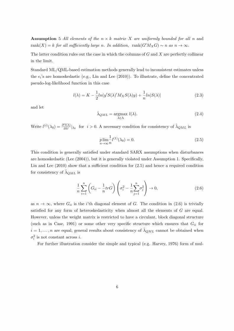
Assumption 5 All elements of the n × k matrix X are uniformly bounded for all n and

rank(X) = k for all sufficiently large n. In addition, rank(G′MXG) ∼ n as n→∞.

The latter condition rules out the case in which the columns of G and X are perfectly collinear

in the limit.

Standard ML/QML-based estimation methods generally lead to inconsistent estimates unless

the εi’s are homoskedastic (e.g., Lin and Lee (2010)). To illustrate, define the concentrated

pseudo-log-likelihood function in this case

l(λ) = K − 1

2ln(y′S(λ)′MXS(λ)y) +

1

nln|S(λ)| (2.3)

and let

λQML = argmaxλ∈Λ

l(λ). (2.4)

Write l(i)(λ0) = ∂il(λ)∂λi|λ0 for i > 0. A necessary condition for consistency of λQML is

p limn→∞

1

nl(1)(λ0) = 0. (2.5)

This condition is generally satisfied under standard SARX assumptions when disturbances

are homoskedastic (Lee (2004)), but it is generally violated under Assumption 1. Specifically,

Lin and Lee (2010) show that a sufficient condition for (2.5) and hence a required condition

for consistency of λQML is

1

n

n∑i=1

(Gii −

1

ntrG

)σ2i −

1

n

n∑j=1

σ2j

→ 0, (2.6)

as n → ∞, where Gii is the i’th diagonal element of G. The condition in (2.6) is trivially

satisfied for any form of heteroskedasticity when almost all the elements of G are equal.

However, unless the weight matrix is restricted to have a circulant, block diagonal structure

(such as in Case, 1991) or some other very specific structure which ensures that Gii for

i = 1, . . . , n are equal, general results about consistency of λQML cannot be obtained when

σ2i is not constant across i.

For further illustration consider the simple and typical (e.g. Harvey, 1976) form of mul-

6

tiplicative heteroskedasticity given by

Ω0(γ) = σ2

ez1γ 0 0 . . . 0

0 ez2γ 0 . . . 0...

.... . .

......

0 0 . . . 0 eznγ

(2.7)

for scalar parameters γ and σ2 and an n-vector of observables z = (z1, . . . , zn)′. Set σ2 = 1

without loss of generality. For Ω0(γ) defined as in (2.7), the LHS of (2.6) becomes

∞∑t=0

γt

t!

1

n

n∑i=1

(Gii −

1

ntrG

)zti − 1

n

n∑j=1

ztj

(2.8)

The latter expression confirms that, even in presence of a very simple form of heteroskedas-

ticity such as that in (2.7), the condition displayed in (2.6) is difficult to check for general

W and z1, ...., zn. Of course, under the extreme condition that the sample covariance be-

tween the diagonal elements of G and zt is zero for each t for n → ∞, then condition (2.6)

holds. But if instead that sample covariance is constant and non-zero across t (at least for

sufficiently large n) the LHS of (2.6) becomes K(eγ − 1), which vanishes only when γ → 0.

Simple calculations confirm that (2.8) is nonzero for other cases. For instance, if Gii, ziare stationary and ergodic over i with mean µG, µz and if zi has finite moment generating

function, then

∞∑t=0

γt

t!

1

n

n∑i=1

(Gii −

1

ntrG

)zti − 1

n

n∑j=1

ztj

→a.s. E(Gii − µG)eγzi, (2.9)

which is non zero whenever the covariance is E(Gii − µG)eγzi is non zero.

Little has, as yet, been said about the bias of λQML under Assumption 1. Starting from

the results in Bao (2013), we may compute the bias of λQML for Ω0(γ) given in (2.7). For

illustration, we limit our analysis to the Gaussian case, although more general results can be

obtained at the expense of extra computation. To assist in the bias calculation we derive the

following explicit moment expressions

E(l(1)(λ0)) =tr(GΩ0(γ))

tr(Ω0(γ))− 1

ntr(G) + o(1), (2.10)

7

E(l(2)(λ0)) = −β′0X′G′MGXβ0 + tr(G′GΩ0(γ))

tr(Ω0(γ))+

2tr2(GΩ0(γ))

tr(Ω0(γ))− 1

ntr(G2) + o(1), (2.11)

E(l(2)(λ0)l(1)(λ0)) =− tr(GΩ0(γ)) (tr(G′GΩ0(γ)) + β0X′G′MGXβ0)

tr2(Ω0(γ))− 1

ntr(G2)

tr(GΩ0(γ))

tr(Ω0(γ))

+1

ntr(G)

tr(G′GΩ0(γ)) + β0X′G′MGXβ0

tr(Ω0(γ))− 2

n

tr2(GΩ0(γ))

tr2(Ω0(γ))+ 2

tr3(GΩ0(γ))

tr3(Ω0(γ))

+1

n2tr(G)tr(G2) + o(1), (2.12)

E(l(3)(λ0)) =− 6tr(GΩ0(γ)) (β′0X

′G′MGXβ0 + tr(G′GΩ0(γ)))

tr2(Ω0(γ))+

8tr3(GΩ0(γ))

tr(Ω0(γ))

− 2

ntr(G3) + o(1) (2.13)

and

E(l(1)(λ0)2) =tr2(GΩ0(γ))

tr2(Ω0(γ))+

1

n2tr2(G)− 2

ntr(G)

tr(GΩ0(γ))

tr(Ω0(γ))+ o(1). (2.14)

Let B(γ, λ0) = E(λQML) − λ0. From these calculations and Bao (2013), we deduce the

following result.

Corollary 1 Let ε be a vector of n independent random variables, normally distributed and

such that E(εε′) = Ω0(γ), where Ω0(γ) is defined in (2.7) with σ2 = 1. Let Assumptions 2-4

hold. The leading term of B(γ, λ0) is given by

B(γ, λ0) =− 2(E(l(2)(λ0))

)−1E(l(1)(λ0)) +

(E(l(2)(λ0))

)−2E(l(2)(λ0)l(1)(λ0))

−1

2

(E(l(2)(λ0))

)−3E(l(3)(λ0))E(l(1)(λ0)2). (2.15)

Under Assumption 1 terms in (2.10), (2.12) and (2.14) do not vanish as n increases,

unless γ = 0 (i.e. the homoskedastic case) and/or some specific structure of W is imposed

which ensures that a condition related to (2.6) holds. Given (2.3), the calculation of (2.10)-

(2.13) is based on the explicit computation of moments of ratio of quadratic form. Most of

the moments of ratios involved are indeed exactly ratio of moments, as ratios of the form

ε′Aε/ε′MXε for a generic n× n matrix A are independent of ε′MXε4. However, since we are

only interested in the leading terms of (2.15), we can approximate moments of ratios as ratios

of moments even when the independence conditions fails. The computation of moments is

standard (Bao and Ullah (2007)) and details are omitted here.

4See, for example, Conniffe and Spencer (2001), for an analysis and history of this result on ratios ofquadratic forms and other moments.

8

In Figure 1, shown in the Appendix, we report plots of B(γ, λ0) for different values of λ0

and for four different choices5 of W against γ ∈ [−10, 10] at n = 200. The elements of the

vector (z1, . . . , zn)′ are generated once from a uniform distribution with support [0, 4] and

kept fixed across γ as well as across different scenarios. For each choice of W , the spatial

parameter ranges from λ0 = −0.8, 0, 0.4, 0.8. The plot depicted on the top left of Figure 1

reports B(γ, λ0) when W is chosen as a block diagonal matrix (Case (1991)). Specifically,

this first choice of W is defined as

Wn = Ir ⊗Bm, Bm =1

m− 1(lml

′m − Im), (2.16)

where Is is the s×s identity matrix, lm is an m-vector of 1’s, and ⊗ is the Kronecker product.

It is easy to verify that the Gii for i = 1, . . . , n are constant across i for W in (2.16). Similarly,

the plot in the top right of Figure 1 reports B(γ, λ0) when W is chosen as a circulant with two

neighbours behind and two ahead. As expected, for both these choices of W the bias function

is zero for all values of λ0 as γ varies. The plot depicted in bottom left of Figure 1 is the

bias function when W is randomly generated as an n×n matrix of zeros and ones, where the

number of “ones” is restricted at 20% of the total number of elements in W . This choice of W

is generated once for any given n and kept fixed across different γ and λ. Similarly, the plot in

the bottom right of Figure 1 displays B(γ, λ0) for W based on an exponential distance decay,

with wij = exp(−|ì − `j |)1(|ì − `j | < log n) where ì is the i−th location along the interval

[0, n], which is randomly generated from Unif [0, n]. Again, we generate one W for each

sample size and we keep it fixed across scenarios. In the sequel, we refer to these matrices as

“random” and “exponential”. Both “random” and “exponential” are then rescaled by their

respective spectral norm, and they tend to be much more relevant to empirical work than

other choices such as (2.16) or circulant matrices, as they mimic contiguity-based weight

matrices. Under either “random” or “exponential”, under Assumption 1, the ML/QML is

not expected to return consistent estimators for a general heteroskedastic design as Gii for

i = 1, . . . , n vary across i.

Figures shown in the bottom panel of Figure 1 confirm that the finite sample bias persists

even for a moderately-sized sample of n = 200 and its magnitude varies with λ0 (e.g. the

bias is in general larger in absolute value for a large negative λ0). Also, the bias tend to

be generally more severe for “exponential” W , as shown in the plot in the bottom right of

Figure 1. As expected from (2.10)-(2.14), the leading terms of (2.15) vanish for λ0 = 0 and

for γ = 0 (although, even if they are not displayed in Figure 1, terms that vanish as n→∞may persist in finite samples and contribute to the overall bias of λQML).

5In figure (7) we depict the structure of the four choices of weight matrices used in the sequel, to illustratethe degree of sparseness and/or symmetry.

9

3 Continuously Updated Indirect Inference based on OLS es-

timates

As discussed in Section 2, in the presence of unknown heteroskedasticity the standard ML/QML

methods are, in general, biased and inconsistent. On the other hand, the OLS estimators

of the unknown parameters in (2.1) can be consistent even under Assumption 1, as long as

some stringent conditions on the asymptotic behaviour of W are satisfied. Specifically, as

shown in Lee (2002), the OLS estimator of λ0 is consistent as long as the sequence h defined

in Assumption 3(iv) diverges, and it is asymptotically normal if√n/h = o(1) as n→∞. For

instance, OLS estimation of (2.1) will lead to inconsistent estimates in situations whereby

the spatial weights are generated via a contiguity criterion (e.g. country borders) and the

number of neighbours of a given unit (country in this case) needs to remain constant as the

sample size increases, regardless of whether homoskedasticity in the disturbances holds or

not.

The limit conditions on h that justify consistency of OLS are hardly verifiable in practical

situations as only a finite set of observations is available in most circumstances and we are

typically agnostic about the limit behaviour of h. So, reasons for using OLS are commonly

and justifiably ignored. On the other hand, OLS can be used as the simple building block

of the new technique developed in the present paper, taking advantage of its computational

simplicity. Our methodology can in principle be extended to QML or other implicitly defined

estimators, at the expense of some additional computational (and algebraic) costs.

Using (2.1) we can “concentrate β out” as

β(λ) = (X′X)−1X

′S(λ)y, (3.1)

and focus on estimation of λ0. The OLS estimator of λ in (2.1), denoted by λ, is defined as:

λ =y′W′MXy

y′W ′MXWy. (3.2)

Similar to the discussion in KPR, we can obtain a formal expansion for the expected value

of the latter ratio based on Lieberman’s (1992) result as

E(λ) =E(y′W ′MXy)

E(y′W ′MXWy)+O

(1

n

). (3.3)

10

Let Q(λ) = MXG(λ), P (λ) = Q(λ)′S−1(λ), Q = Q(λ0) and P = P (λ0). By standard algebra

E(λ) =tr(PΩ0) + β′0X

′PXβ0

tr(Q′QΩ0) + β′0X′Q′QXβ0

+O

(1

n

). (3.4)

Following the formal expansion in (3.4), we define the binding function τn(λ) as

τn(λ,Ωλ, β(λ)) = τn(λ) =tr(P (λ)Ωλ) + β(λ)′X ′P (λ)Xβ(λ)

tr(Q(λ)′Q(λ)Ωλ) + β(λ)′X ′Q(λ)′Q(λ)Xβ(λ)+Op

(1

n

), (3.5)

and its approximate counterpart (which will be used for practical implementation) as

τ∗n(λ,Ωλ, β(λ)) = τ∗n(λ) =tr(P (λ)Ωλ) + β(λ)′X ′P (λ)Xβ(λ)

tr(Q(λ)′Q(λ)Ωλ) + β(λ)′X ′Q(λ)′Q(λ)Xβ(λ), (3.6)

with β(λ) defined according to (3.1), and

Ωλ = diag(ε(λ)ε(λ)′), ε(λ) = (y − λWy −Xβ(λ)), (3.7)

where diag(A) for a generic n×n matrix A returns an n×n diagonal matrix containing only

the main diagonal of A and whose other entries are zero.

Our new continuously updated indirect inference (CUII) estimator of λ, λCUII is defined

as

λCUII = argminλ ∈ Λ

λ− τn(λ,Ωλ, β(λ))2. (3.8)

A detained discussion on the robustness advantages of using τ∗n(.) rather than its standard

simulated version (e.g. Gourieroux et al. (2000)) is contained in KPR. In this setting, the

standard II approach of simulating pseudo-data to construct the binding function would re-

quire even more structure compared to standard estimation problems under homoskedasticity,

as not only distributional assumptions, but also the specification of the form of heteroskedas-

ticity would be necessary. From substantial numerical work the objective function in (3.8) is

found to be continuous and strictly convex for all values of the parameter space, so that the

optimization problem appears to be standard. Since smoothness and monotonicity conditions

on τn(λ) are imposed to establish the limit theory, we introduce the following conditions.

Assumption 6

(i) For all n, τn(λ) is continuously differentiable and strictly increasing for all λ ∈ Λ with

probability one.

(ii) p lim τ(1)n

n→∞(λ0) exists and is positive.

11

As discussed in KPR, the latter is employed as a high-level condition because the deriva-

tion of more primitive assumptions involving general choices of W is not feasible. KPR

verified a condition similar to Assumption 6 for a class of W with Toeplitz structures (e.g.

circulant and block diagonal structures). However, as is common practice in the simulation-

based techniques literature, when W has a more general unspecified structure practitioners

have to rely on numerical methods to verify Assumption 6. Under Assumption 6, we have

the inverse function representation of the CUII estimator

λCUII = τ−1n (λ). (3.9)

4 Limit Theory

This section derives the asymptotic properties of the estimator (3.8) for model (2.1) when

the case β0 = 0 a priori is ruled out. From (3.5) and (3.6) we consider the centring random

sequence

τn(λ0) =tr(G′MXS

−1Ωλ0)/n+ β(λ0)′X ′S−1′W ′MXS−1Xβ(λ0)/n

tr(G′MXGΩλ0)/n+ β(λ0)′X ′G′MXGXβ(λ0)/n+O

(1

n

)=

tr(PΩλ0)/n+ β(λ0)′X ′PXβ(λ0)/n

tr(Q′QΩλ0)/n+ β(λ0)′X ′Q′QXβ(λ0)/n+O

(1

n

), (4.1)

where

β(λ0) = β0 + (X ′X)−1X ′ε, (4.2)

ε(λ0) = MXε, (4.3)

so that Ωλ0 = diag(MXεε′MX).

Define

Vn =4

n

(β′0X

′P ′MXΩ0MXPXβ0 β′0X′P ′MXΩ0MXQ

′QXβ0

β′0X′Q′QMXΩ0MXPXβ0 β′0X

′Q′QMXΩ0MXQ′QXβ0

)

+4

n

∑i

∑j<i

σ2i σ

2j

((P+P ′)2ij

4(P+P ′)ij(Q′Q)ij


2 (Q′Q)2ij

). (4.4)

In order to assure the existence of each limit appearing in (4.4) we impose

Assumption 7 As n→∞, limVn exists.

12

Also, define the limits

a = a(λ0) = limn→∞

1

ntr(PΩ0), b = b(λ0) = lim

n→∞

1

nβ0X

′PXβ0,

c = c(λ0) = limn→∞

1

ntr(Q′QΩ0), d = d(λ0) = lim

n→∞

1

nβ′0X

′Q′QXβ0 (4.5)

and

a(1) = a(1)(λ0) = limn→∞

1

ntr(G′PΩ0 + PGΩ0),

b(1) = b(1)(λ0) = limn→∞

1

n

(β′0X

′(G′P + PG)Xβ0 − 2β′0X′P (I −MX)GXβ0

),

c(1) = c(1)(λ0) = limn→∞

2

ntr(G′Q′QΩ0),

d(1) = d(1)(λ0) = limn→∞

2

n(β′0X

′G′Q′QXβ0 − β′0X ′Q′Q(I −MX)G′Xβ0) (4.6)

so that

τ (1) = τ (1)(λ0) = plim τ (1)n

n→∞(λ0) =

a(1) + b(1)

c+ d− (c(1) + d(1))(a+ b)

(c+ d)2, (4.7)

whose existence and non-singularity is assured by Assumption 6.

By virtue of the delta method

√n(λ− τn(λ0)) = f ′nUn + op (1) , (4.8)

where

Un =1√n

(ε′Pε− tr(PΩλ0) + 2β′0X

′P ′MXε

ε′Q′Qε− tr(Q′QΩλ0) + 2β′0X′Q′QMXε

)(4.9)

and

fn =

((1

ny′W ′MXWy

)−1

;

(1

ny′W ′MXWy

)−2( 1

ny′W ′MXy

))′. (4.10)

We derive

f = plim fnn→∞

=((c+ d

)−1;(c+ d

)−2 (a+ b

))′, (4.11)

which is defined in terms of limits appearing also in τ (1). Thus, its existence and non singu-

larity is assured under Assumption 6.

With these results in hand, we obtain the following limit theory.

13

Theorem 1

(a) Under (2.1) with β0 6= 0 and Assumptions 1-7

√n(λ− τn(λ0))→

dN (0, f ′ lim

n→∞Vnf). (4.12)

(b) Under (2.1) with β0 6= 0 and Assumptions 1-7

√n(λCUII − λ0)→

dN(0, v2

CUII

), (4.13)

where v2CUII = f ′ lim

n→∞Vnf/

(τ (1)

)2exists and is non zero under Assumptions 2, 3(ii)

and 5-7.

Let v2CUII be the estimated version of v2

CUII , obtained by replacing the unknown λ0 and β0

by λCUII and βCUII , respectively, Ω0 by Ω = diag(εε′) where ε = MXS(λCUII)y, and σ2i

replaced by ε2i , for i = 1, ....., n.

Theorem 2 Let Assumption 1 hold, with δ = 2. Under Assumptions 2-7, as n→∞

v2CUII − v2

CUII →p 0. (4.14)

The proofs of Theorems 1 and 2 are given in the Appendix.

Estimation of β0 in 2.1 under Assumption 1 is generally less problematic than estimation

of λ0 as simple OLS produces consistent estimates under general limit behaviour of W .

Nonetheless, from (3.1) we can deduce consistency of βCUII and its asymptotic normality by

using the representation

√n(βCUII − β0) =

(1

nX ′X

)−1 1√nX ′ε−

(1

nX ′X

)−1 1

nX ′GXβ0

√n(λCUII − λ0) + op(1),

(4.15)

where√n(λCUII − λ0) =

1

τ(1)n (λ0)

√n(λ− τn(λ0)) + op(1). (4.16)

From (4.8), (4.9) and (4.10)√n(βCUII − β0) = ζ ′nRn, (4.17)

14

where

Rn =1√n

X ′ε

ε′Pε− tr(PΩλ0) + 2β′0X′P ′MXε


(4.18)

and

ζn =

((1

nX ′X

)−1

; −(

1

nX ′X

)−1 1

nX ′GXβ0τ

(1)n (λ0)−1f ′n

)′(4.19)

Defining

ζ = plimn→∞

ζn, (4.20)

and

Tn =1

n

X ′X X ′Ω0MX(P + P ′)Xβ0 2X ′Ω0MXQ

′QXβ0

β′0X′(P + P ′)MXΩ0X 4β′0X

′P ′MXΩ0MXPXβ0 4β′0X′P ′MXΩ0MXQ

′QXβ0

2β′0X′Q′QMXΩ0X 4β′0X

′Q′QMXΩ0MXPXβ0 4β′0X′Q′QMXΩ0MXQ

′QXβ0

+4

n

∑i

∑j<i

σ2i σ

2j

0(k×k) 0(k×1) 0(k×1)

0(1×k)(P+P ′)2ij


2

0(1×k)(P+P ′)ij(Q′Q)ij

2 (Q′Q)2ij

, (4.21)

we deduce the following result.

Corollary 2 Under (2.1) with β0 6= 0, under Assumptions 1-7

√n(βCUII − β0)→

dN (0, ζ ′ lim

n→∞Tnζ), (4.22)

as n→∞.

The variance-covariance matrix ζ ′ limn→∞

Tnζ exists and is non-singular under Assumptions 5-7.

The proof of Corollary 2 follows in a similar way to that of part (a) of Theorem 1 and is

omitted.

5 Simulations

We conduct a set of Monte Carlo experiments to compare the finite sample performance of the

CUII estimators with the standard QML and OLS estimators, as well as to the robust GMM

(RGMM, henceforth) of Lin and Lee (2010) and to the modified QML (MQML, henceforth)

of Liu and Yang (2015).

We consider different scenarios for our simulation exercise, and for each design the number

15

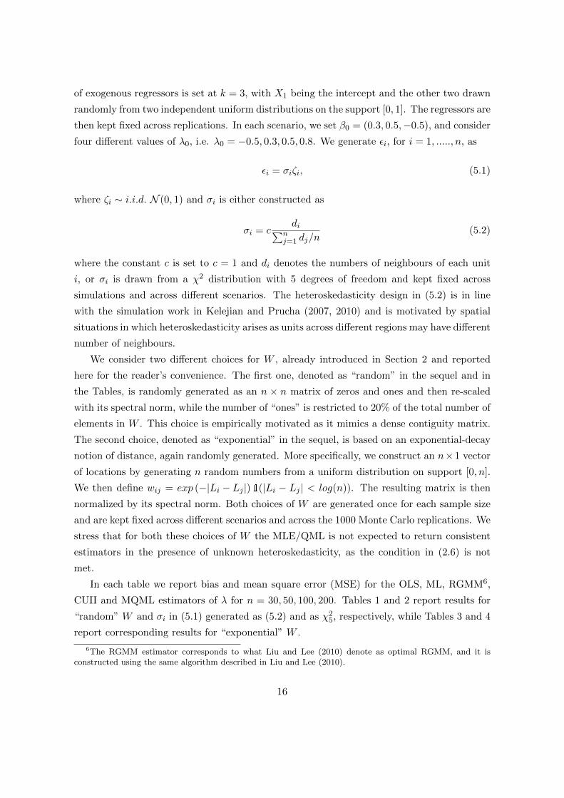
of exogenous regressors is set at k = 3, with X1 being the intercept and the other two drawn

randomly from two independent uniform distributions on the support [0, 1]. The regressors are

then kept fixed across replications. In each scenario, we set β0 = (0.3, 0.5,−0.5), and consider

four different values of λ0, i.e. λ0 = −0.5, 0.3, 0.5, 0.8. We generate εi, for i = 1, ....., n, as

εi = σiζi, (5.1)

where ζi ∼ i.i.d. N (0, 1) and σi is either constructed as

σi = cdi∑n

j=1 dj/n(5.2)

where the constant c is set to c = 1 and di denotes the numbers of neighbours of each unit

i, or σi is drawn from a χ2 distribution with 5 degrees of freedom and kept fixed across

simulations and across different scenarios. The heteroskedasticity design in (5.2) is in line

with the simulation work in Kelejian and Prucha (2007, 2010) and is motivated by spatial

situations in which heteroskedasticity arises as units across different regions may have different

number of neighbours.

We consider two different choices for W , already introduced in Section 2 and reported

here for the reader’s convenience. The first one, denoted as “random” in the sequel and in

the Tables, is randomly generated as an n × n matrix of zeros and ones and then re-scaled

with its spectral norm, while the number of “ones” is restricted to 20% of the total number of

elements in W . This choice is empirically motivated as it mimics a dense contiguity matrix.

The second choice, denoted as “exponential” in the sequel, is based on an exponential-decay

notion of distance, again randomly generated. More specifically, we construct an n×1 vector

of locations by generating n random numbers from a uniform distribution on support [0, n].

We then define wij = exp (−|Li − Lj |)1(|Li − Lj | < log(n)). The resulting matrix is then

normalized by its spectral norm. Both choices of W are generated once for each sample size

and are kept fixed across different scenarios and across the 1000 Monte Carlo replications. We

stress that for both these choices of W the MLE/QML is not expected to return consistent

estimators in the presence of unknown heteroskedasticity, as the condition in (2.6) is not

met.

In each table we report bias and mean square error (MSE) for the OLS, ML, RGMM6,

CUII and MQML estimators of λ for n = 30, 50, 100, 200. Tables 1 and 2 report results for

“random” W and σi in (5.1) generated as (5.2) and as χ25, respectively, while Tables 3 and 4

report corresponding results for “exponential” W .

6The RGMM estimator corresponds to what Liu and Lee (2010) denote as optimal RGMM, and it isconstructed using the same algorithm described in Liu and Lee (2010).

16

[Tables 1-4 about here]

As expected, since our choices of W do not satisfy the limit condition for OLS consistency,

the OLS results are severely biased for all sample sizes and across all scenarios. A similar

comment holds for the ML estimate of λ, which displays severe bias that does not improve

as n increases in the ‘random’ W case, whereas for the ‘exponential’ W case, the bias of the

ML estimate is severe for small n but appears to decrease with sample size.

The performance of λCUII has to be compared to its counterparts that are robust to

heteroskedasticity. Across different scenarios, we can see that bias and MSE of λCUII is

comparable to results obtained by MQML, and outperforms MQML in terms of MSE for most

values of λ0 and n for the ‘random’ W case. Moreover, from a computational perspective,

CUII appears easier to implement and is much less sensitive to the (arbitrary) starting value

of the optimization routine. Tables 1 and 2 reveal poor performance of RGMM, which suffers

from severe bias even for moderate sample sizes. This behaviour is probably due to the

fact that ‘random’ W is a dense choice of weighting matrix, where standard GMM types of

procedures do not perform well in small-moderate samples. The bias appears to decrease

with n, confirming the asymptotic properties of RGMM in presence of heteroskedastic errors.

In the ‘exponential’ W case, the performance of RGMM is poor for small sample sizes and

improves for n = 100 but its finite sample performance remains inferior to that of CUII and

MQML.

6 Empirical Illustration

In this section we report an empirical application of the CUII estimator and compare results

to those obtained by the competitor methods QML, RGMM and MQML. This application

provides an illustration of the new method in a practical setting. The application is com-

plemented by a further simulation that is matched to the empirical data and therefore more

realistic of typical implementations than standard Monte Carlo designs.

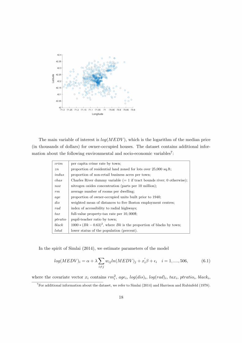
Specifically, we use the Boston house price data (Harrison and Rubinfeld (1978)) and its

‘corrected’ version (Gilley and Pace, 1996), which also includes information on LON (tract

point longitudes in decimal degrees and LAT (tract point latitudes in decimal degrees) for

the 506 census tracts in the Boston Standard Metropolitan Area during the early 1970s. The

locations of the 506 census tracts are depicted in the figure below.

17

-71.3 -71.25 -71.2 -71.15 -71.1 -71.05 -71 -70.95 -70.9 -70.85 -70.8

Longitude

42

42.05

42.1

42.15

42.2

42.25

42.3

42.35

42.4L

atitu

de

The main variable of interest is log(MEDV ), which is the logarithm of the median price

(in thousands of dollars) for owner-occupied houses. The dataset contains additional infor-

mation about the following environmental and socio-economic variables7:

crim per capita crime rate by town;

zn proportion of residential land zoned for lots over 25,000 sq.ft;

indus proportion of non-retail business acres per town;

chas Charles River dummy variable (= 1 if tract bounds river; 0 otherwise);

nox nitrogen oxides concentration (parts per 10 million);

rm average number of rooms per dwelling;

age proportion of owner-occupied units built prior to 1940;

dis weighted mean of distances to five Boston employment centres;

rad index of accessibility to radial highways;

tax full-value property-tax rate per 10, 000$;

ptratio pupil-teacher ratio by town;

black 1000 ∗ (Bk − 0.63)2, where Bk is the proportion of blacks by town;

lstat lower status of the population (percent).

In the spirit of Simlai (2014), we estimate parameters of the model

log(MEDV )i = α+ λ∑i 6=j

wijln(MEDV )j + x′iβ + εi i = 1, ...., 506, (6.1)

where the covariate vector xi contains rm2i , agei, log(dis)i, log(rad)i, taxi, ptratioi, blacki,

7For additional information about the dataset, we refer to Simlai (2014) and Harrison and Rubinfeld (1978).

18

log(stat)i, crimi, zni, indusi, chasi, nox2i . When λ = 0 ex-ante, the model simplifies to the

hedonic price model. Since the main scope of this paper is robust estimation and inference on

λ, this illustration focuses on the spatial network effect in model (6.1) and thus on estimation

and significance of λ, rather than the covariate coefficient vector β. We recall that estimation

of β in the general model (2.1) and in the specific model (6.1) poses fewer consistency and

efficiency issues compared to inference on λ. Empirical results for the estimates of the β

coefficients in the various weight matrix scenarios can be obtained from the authors.

We conjecture that several measure of proximity might play a role in the house price

determination process of MEDVi, so that both economic distance and geographical distance

seem relevant. Accordingly we design five different choices of weight matrix W , which are

denoted respectively as W geo, W exp,geo, W geo,0.9, W tax and W school. The first three choices

for W in (6.1) reflect geographical proximity and rely on the geo-distance between tract i

and j (denoted as geoij in the sequel) computed using the Haversine formula. The matrices

W geo, W exp,geo and W geo,0.9 are then constructed as

• W geo: wij = 1/geoij ;

• W geo,exp: wij = exp (−|geoij |)1(|geoij | < log(n));

• W geo,0.9: wij = 1(|geoij | < D∗), where we set D∗ = 2.5 km to obtain a matrix

sparseness of approximately 9%.

The remaining two choices of W are defined in terms of various economic distances.

W tax contains the inverse of pairwise distances between census tracts, where proximity is

defined according to how similar their respective full-property tax rates are. Specifically

wtaxij = 1/|taxi − taxj | if taxi 6= taxj , and wtaxij = 1 if taxi = taxj . Heuristically, we

expect house prices to be affected more from the house prices of neighbouring properties,

where ‘neighbour’ is now defined as being of similar status, which in turn is proxied by the

property tax rate. Similarly, we define W school based on the observable ptratio, which it is

known to reflect the quality of schools in each census tract. Again, two census tracts with

similar ptratio are expected to be similar in terms of their socio-economic status. We define

wschoolij = 1/|ptratioi − ptratioj |, as long as ptratioi 6= ptratioj , and wschoolij = 1 in case

ptratioi = ptratioj . For all choices of W we set wii = 0 and we normalize the matrices so

that elements of each row sum to 1.

19

QML CUII RGMM MQML

W geo λ 0.0399 0.0426 0.0442 0.0391

t-ratio 1.2543 14.6806 1.2595 2.6462

W exp,geo λ 0.0546 0.0665 0.0657 0.0563

t-ratio 2.7419 7.3380 3.9306 11.4364

W geo,0.9 λ 0.0130 0.0131 0.0127 0.0132

t-ratio 2.4790 44.7070 3.0448 72.5195

W tax λ 0.0217 0.0230 0.0143 0.0235

t-ratio 1.2368 12.3797 1.0886 12.7909

W school λ -0.0269 -0.0268 -0.0271 -0.0268

t-ratio -2.9089 -91.3553 -2.3550 -17.9526

Table 5: Estimates and t-statistic of λ in (6.1) computed by QML, CUII, RGMM and MQML

for different choices of weighting structures.

In Table 5 we report estimates and t-ratios for the parameter λ obtained by QML, CUII,

RGMM and MQML. The estimates of λ do not vary much across QML, CUII, MQML and

RGMM, the main exception being that the estimates obtained by CUII and RGMM are

slightly larger than those obtained by QML and MQML when the weight matrix W geo is

adopted in (6.1). But a major difference between the methods shows up in the significance

of the spatial effects. The methods CUII and MQML return similar results with highly

significant t-statistics in all scenarios, with t-statistics substantially larger by an order of

magnitude than those of the other methods. The effects of robustification to heterogeneity

in the equation errors is therefore materially important in hypothesis testing.

The t-statistics obtained by QML are unreliable because the QML standard errors are

not robust to heteroskedasticity of the errors, but the corresponding figures are reported in

the tables for completeness. Finally, the t−ratios obtained by RGMM are not significant

for the weighting structures W tax and W geo, a result that contrasts sharply with the robust

estimators.

In order to assess the accuracy, and hence the reliability of point estimates and t-statistics

displayed in Table 5, we mimic the empirical illustration in a Monte Carlo exercise by means

of B bootstrap samples constructed from the point estimates in Table 5 and using a wild

bootstrap variant to generate simulation errors from the actual residuals. Specifically, we de-

note by εN , for N = QML,CUII,RGMM,MQML, the vector of residuals based on figures

in Table 5, and we generate a n × B matrix of i.i.d random variables from the Rademacher

20

distribution, with typical element indicated by rij for i = 1, .....n and j = 1, ....B. For each

estimator N and each choice of W we then generate B sets of pseudo-data vectors as

y∗N,j = S−1(λN )(XβN + u∗N,j

), j = 1, ....., B, (6.2)

with each component of u∗N,j being constructed as u∗N,ij = (n/(n−k))1/2εN,irij (k = 14), and

we calculate the corresponding B estimators λ∗N,j , for j = 1, ...., B, so that a measure of bias

and MSE can be computed as

BiasN =1

B

B∑j=1

λ∗N,j − λN , MSEN = Bias2N +

1

B

B∑j=1

λ∗N,j − 1

B

B∑j=1

λ∗N,j

2

. (6.3)

Results of this bootstrap exercise are reported in Table 6. For ease of interpretation, given

the small magnitude of λN for N = QML,CUII,RGMM,MQML, in Table 6 we report

scaled quantities, i.e. BiasN/λN and MSEN/λ2N .

QML CUII RGMM MQML

W geo BiasN/λN -0.0007 0.0646 0.0546 0.0691

MSEN/λ2N 0.9204 0.8136 0.7645 0.9678

W exp,geo BiasN/λN -0.2344 -0.0095 -0.0220 -0.0386

MSEN/λ2N 0.1452 0.0618 0.0642 0.1647

W geo,0.9 BiasN/λN 0.0465 0.0525 0.0554 0.0523

MSEN/λ2N 0.1277 0.1268 0.1313 0.1259

W tax BiasN/λN -0.0967 -0.0382 -0.0610 -0.0359

MSEN/λ2N 0.4461 0.3658 0.9324 0.3888

W school BiasN/λN -0.0154 -0.0199 -0.0176 -0.0201

MSEN/λ2N 0.1817 0.1732 0.1816 0.1840

Table 6: Bias and MSE for N = QML,CUII,RGMM,MQML computed from B = 100

bootstrap samples for various choices of weighting structures.

Results in Table 6 confirm that λCUII has a better performance in terms of bias and/or

MSE than its robust counterparts RGMM and MQML for several choices of W . Again,

QML is not expected to be consistent in these scenarios, although its bias appears to be

substantially larger than that of other estimators only for W exp,geo. More importantly, the

clear advantage in terms of efficiency of λCUII and λMQML over λRGMM outlined in Table

21

5 for W tax, is confirmed by the simulation exercise reported in Table 6. However, this small

simulation exercise reveals that results obtained when proximity is defined as W geo are very

erratic, and thus practitioners should treat estimates and tests reported in the first line

of Table 5 as not particularly reliable. This behaviour is probably due to the very dense

structure of this choice of weighting structure. Results for W geo,0.9 and W school reported in

Table 6 partially confirms those in Table 5, as MSECUII and MSEMQML are lower than

MSERGMM , but the comparative advantage in terms of MSE does not fully match the

considerable difference in their t-statistic values reported in Table 5.

While the main goal of this empirical exercise is to illustrate the implementation of the

CUII method in relation to other spatial econometric methods, the results do reveal some

interesting features concerning the various channels of spatial correlation in the context of

house price determination. In particular, it seems worthy of mention that spatial effects that

are present when the network structure is defined in terms of W tax or W school continue to

persist when the individual levels of tax and ptratio are included among regressors, revealing

a genuinely significant impact. It is also worth pointing out that the spatial effects induced

by W tax and W school differ in sign and thus their interpretation as positive or negative spatial

spillovers differ, an empirical feature that might usefully be explored in subsequent research.

7 Concluding Remarks

Unobserved heteroskedasticity in the disturbances is a frequent occurrence in spatial models

due to sample unit heterogeneity across their many individual features, including respective

unit size. The new estimation method introduced in this paper directly addresses such het-

erogeneity, relying on an indirect inference transformation of standard OLS estimation that

parametrizes the error covariance matrix in terms of the unknown spatial parameter. The

procedure follows in the spirit of continuously updated estimators in the broader economet-

ric literature such as GMM. The resulting CUII estimator is consistent and asymptotically

normal under some standard model and regularity conditions combined with an additional

binding function condition that can be numerically verified in practical work.

The finite sample performance of the CUII estimator is found in simulations to be very

satisfactory when compared to other robust methods such as the GMM robust procedures of

Lin and Lee (2010) and Kelejian and Prucha (2010) or the modified QMLE procedure of Liu

and Yang (2015). Implementation of CUII is straightforward and the optimization routine

to derive the estimator appears to converge quickly even when an artificially dense W matrix

is designed. A simple empirical illustration based on Boston house price data reveals that a

major advantage of accommodating heterogeneity in system disturbances lies in hypothesis

22

testing, where significance tests are found to differ considerably across estimation methods,

with CUII giving much higher levels of significance to spatial effects across many different

choices of the house price network structure.

Appendix

Proof of Theorem 1.

Proof of part (i) Let ψij and ψij be the 2 × 1 vectors defined as ψij = ( ψ1ij ψ2ij )′ =

( (P + P ′)ij/2 (Q′Q)ij )′ and ψij = ( ψ1ij ψ2ij )′ = ( (MXP )ij (MXQ′Q)ij )′, respec-

tively.

Let Ω = diag(εε′) and Ωλ0 = diag(MXεε′MX), consonant with the notation of Section 4.

We first show

Un =1√n

(ε′Pε− tr(PΩλ0) + 2β′0X

′P ′MXε


)

=1√n

(ε′Pε− tr(P Ω) + 2β′0X

′P ′MXε

ε′Q′Qε− tr(Q′QΩ) + 2β′0X′Q′QMXε

)+ op(1). (A.1)

Thus, we need to show

1√n

n∑i=1

ψii,s(εi(λ0)2 − ε2i ) = op(1), s = 1, 2 (A.2)

where εi(λ0) = εi −∑n

i Bijεj , Bij = X ′i(X′X)−1Xj .

We have

1√n

∑i

ψii,s(εi(λ0)2 − ε2i ) =1√n

∑i

ψii,s∑j

∑t

εjεtBijBit −2√n

∑i

ψii,sεi∑j

Bijεj

=1√n

∑i

ψii,s∑j

ε2jB2ij +

1√n

∑i

ψii,s∑j

∑t6=j

εjεtBijBit

− 2√n

∑i

ψii,sε2iBii −

2√n

∑i

ψii,sεi∑j 6=i

Bijεj . (A.3)

The modulus of the first term in (A.3) has expectation bounded by

C√n

∑i

|ψii,s|∑j

B2ij ≤

C√nh

∑i

∑j

B2ij =

C√nhtr(X(X ′X)−1X ′) = o(1) (A.4)

23

as ψii,s = O(1/h) under Assumptions 3 and 4. Similarly, the modulus of the third term has

expectation bounded by

C√n

∑i

|ψii,s|Bii ≤C√nh

∑i

Bii = o(1). (A.5)

The second term is (A.3) has mean zero and variance bounded by

C

n

∑i

∑v

∑j

∑t6=j|ψii,s||ψvv,s||BijBitBvtBvj | ≤

C

n

∑i

∑v

∑j

∑t

|ψii,s||ψvv,s||BijBitBvtBvj |

≤ C

nh2

∑i

∑v

∑j

∑t

|BijBit|(B2vt +B2

vj) ≤C

nh2supi

∑j

|Bij |supt

∑i

|Bit|∑v

∑t

B2vt

+C

nh2supj

∑i

|Bij |supi

∑t

|Bit|∑v

∑j

B2vj ≤

C

nh2, (A.6)

under Assumptions 3-5. Similarly, the fourth term in (A.3) has mean zero and variance

bounded by

C

n

∑i

∑j 6=i

ψ2ii,sB

2ij +

C

n

∑i

∑j 6=i

ψii,sψjj,sBijBji ≤C

nh2

∑i

∑j

B2ij ≤

C

nh2. (A.7)

Then (A.2) holds by the Markov inequality.

The rest of the proof is similar to KPR (2017). In order to avoid repetition we refer to

their proof when steps follow in a similar way. Define

ui = ( u1i u2i )′ = 2εi∑j

ψijX′jβ0 + 2εi

∑j<i

ψijεj , (A.8)

so that Un =∑n

i=1 ui + op(1), according to (A.1). The ui, 1 ≤ i ≤ n, n = 1, 2, ..... form a

triangular array of martingale differences with respect to the filtration formed by the σ-field

generated by εj ; j < i. Let

A =V ar

(n∑i=1

ui

)= 4

n∑i=1

σ2i

n∑j=1

n∑t=1

ψijX′jβ0β

′0Xtψ

′it + 4

n∑i=1

∑j<i

σ2i σ

2jψijψ

′ij . (A.9)

Define zin = η′A−1/2ui, where η is a 2× 1 vector satisfying η′η = 1. By Theorem 2 of Scott

(1973)∑n

i zin →d N (0, 1) if the following stability and Lindeberg conditions hold:

n∑i=1

E(z2in|εj ; j < i)

p→ 1, (A.10)

24

andn∑i=1

E(z2in1(|zin > ξ|))→ 0 ∀ξ > 0. (A.11)

As n→∞,

A/n→ limn→∞

Vn, (A.12)

where

Vn =4

n

(β′0X

′P ′MXΩ0MXPXβ0 β′0X′P ′MXΩ0MXQ

′QXβ0

β′0X′Q′QMXΩ0MXPXβ0 β′0X

′Q′QMXΩ0MXQ′QXβ0

)

+4

n

∑i

∑j<i

σ2i σ

2j

((P+P ′)2ij



2 (Q′Q)2ij

)= C1 + C2, . (A.13)

where C1 and C2 contain the first and second terms in (A.13), respectively. All terms in

C1 are O(1), while those in C2 are bounded by O(1/h) under Assumptions 3 and 4, and by

standard algebra. Existence of limits in (A.13) is guaranteed under Assumption 7, and non

singularity of C1 is ensured by Assumptions 2, 3(ii) and 5. The expression in (4.4) is obtained

from (A.13) after routine calculations. Thus, we can replace A by n when showing (A.10)

and (A.11).

We start by establishing (A.10), which can equivalently be written as∑i

E(z2in|εj , j < i

)− η′A−1/2AA−1/2η →

p0. (A.14)

The latter, by standard manipulations and (A.12), is equivalent to showing

4

nη′

∑i

σ2i

∑j<i

εjψij

∑j<i

εjψij

′ −∑i

∑j<i

σ2i σ

2jψijψ

′ij

η →p

0, (A.15)

and

4

nη′

∑i

∑j

∑t<i

σ2i β′0Xj

(ψijψ

′it + ψitψ

′ij

)εt

η →p

0 (A.16)

as n→∞.

In order to avoid replications, we omit the proof of (A.15), referring to KPR and observing

that

||P ||∞ + ||P ′||∞ < K, ||Q||∞ + ||Q′||∞ <∞ (A.17)

25

and both Pij and Qij , for i, j = 1, ...., n, are uniformly bounded by O(1/h), so that ψ1ij and

ψ2ij have, respectively, similar asymptotic properties to (G+G′)ij/2 and (G′G)ij appearing

in the proof of Theorem 1 in KPR. We verify (A.16) by examining the convergence of each

typical element, i.e. by showing

1

n

∑i

∑j

∑t<i

σ2i β′0Xjψsijψvitεt →

p0 (A.18)

for each s, v = 1, 2. Under Assumption 5, i.e. for uniformly bounded Xij for i, j = 1, ...., n,

the LHS of (A.18) has mean zero and variance bounded by

1

n2K|∑i

∑j

∑u

∑h

∑t<i,u

ψsijψsuhψvitψvut| ≤1

n2K∑i

∑j

∑u

∑h

∑t

|ψsijψsuhψvitψvut|

1

nK sup

0<i≤n

∑j

|ψsij | sup0<u≤n

∑h

|ψshu| sup0<t≤n

∑i

|ψvit| sup0<u≤n

∑t

|ψvut| = O

(1

n

), (A.19)

since (A.17) holds and

||MXP ||∞ + ||P ′MX ||∞ < K, ||MXQ′Q||∞ + ||Q′QMX ||∞ <∞ (A.20)

In order to prove (A.11) we verify the sufficient Lyapunov condition

n∑i=1

E|zin|2+δ → 0 (A.21)

by considering a typical standardized element of ui, i.e.∑

iE|(1/n)1/2usi|2+δ for s = 1, 2.

Under Assumption 1, using∑

iE|usi|2+δ =∑

iE(E|usi|2+δ|εj , j < i)) and the cr inequality,

(1

n

)1+δ/2∑i

E|usi|2+δ ≤(

1

n

)1+δ/2

K∑i

E|∑j<i

ψsijεj |2+δ +

(1

n

)1+δ/2

K∑i

|∑j

β′0Xjψsij |2+δ.

(A.22)

Convergence to zero of the first term at the RHS of (A.22) can be shown as in KPR. Con-

vergence of the third term at the RHS of (A.22) can be shown after observing that

|∑j

β′0Xjψsij |2+δ ≤ K sup0<j≤n

|β′0Xj |2+δ∑j

|ψsij |2+δ, (A.23)

where β′0Xj is uniformly bounded under Assumption 5. Thus, the second term at the RHS

26

of (A.22) is bounded by

(1

n

)1+δ/2

K∑i

∑j

|ψsij |2+δ ≤(

1

n

)1+δ/2

K∑i

∑j

ψ2sij

1+δ/2

≤(

1

n

)1+δ/2

K

supi

∑j

ψsij

δ/2∑i

∑j

ψ2sij = O

(1

n

)δ/2(A.24)

similarly to KPR, under Assumptions 3-5.

Thus, A−1/2∑

i ui →dN (0, I), and the statement in Theorem 1(i) follows by standard

delta arguments.

Proof of part (ii). Again, we proceed similarly to KPR and we refer to their proof to avoid

repetitions. We rewrite the binding function τn(λ) as

τn(λ,Ωλ, β(λ)) =tr(P (λ)Ωλ) + β(λ)′X ′P (λ)Xβ(λ)

tr(Q(λ)′Q(λ)Ωλ) + β(λ)′X ′Q(λ)′Q(λ)Xβ(λ)+Op

(1

n

)=a(λ) + b(λ)

c(λ) + d(λ)+Op

(1

n

), (A.25)

where

a(λ) =1

ntr(P (λ)Ωλ), b(λ) =

1

nβ(λ)′X ′P (λ)Xβ(λ), c(λ) =

1

ntr(Q(λ)′Q(λ)Ωλ),

d =1

nβ(λ)′X ′Q(λ)′Q(λ)Xβ(λ). (A.26)

We write

τ (1)n (λ) =

a(1)(λ) + b(1)(λ)

c(λ) + d(λ)− (c(1)(λ) + d(1)(λ))(a(λ) + b(λ))

(c(λ) + d(λ))2+O

(1

n

), (A.27)

where

a(1)(λ) =1

ntr(G′(λ)P (λ)Ωλ) +

1

ntr(P (λ)G(λ)Ωλ) +

1

ntr(PΩ

(1)λ ),

b(1)(λ) = − 2

ny′W ′(In −MX)P (λ)Xβ(λ) +

1

nβ(λ)′X ′G(λ)′P (λ)Xβ(λ) +

1

nβ(λ)′X ′P (λ)G(λ)Xβ(λ),

c(1)(λ) =2

ntr(G(λ)′Q(λ)′Q(λ)Ωλ) +

1

ntr(Q(λ)′MXQ(λ)Ω

(1)λ ),

d(1)(λ) = − 2

ny′W ′(I −MX)Q(λ)′Q(λ)Xβ(λ) +

2

nβ(λ)′X ′G(λ)′Q(λ)′Q(λ)Xβ(λ) (A.28)

27

and

Ω(1)λ = −2diag(MXWyε(λ)′). (A.29)

Since

λCUII − λ0 = τ−1n (λ)− τ−1

n (τn(λ0)), (A.30)

we can derive the limit distribution of√n(λCUII − λ0) by the delta method, as long as the

asymptotic local relative equicontinuity condition (Phillips, 2012) holds. Thus, similar to

KPR, we need to show ∣∣∣∣∣τ (1)n (λ0)− τ (1)

n (r)

τ(1)n (r)

∣∣∣∣∣→p 0 (A.31)

as n → ∞, uniformly in Nδ = r ∈ < : |s(r − λ0)| < δ, δ > 0, s = sn → ∞ and

s(1/n)1/2 → 0. Under Assumption 6(ii), the expression on the LHS of (A.31) is bounded by

K∣∣∣τ (1)n (λ0)− τ (1)

n (r)∣∣∣ , (A.32)

which by the mean value theorem is in turn bounded by

K∣∣∣τ (2)n (λ∗)(λ0 − r)

∣∣∣ , (A.33)

where λ∗ is an intermediate point between λ0 and r. The expression in (A.33) is Op(|λ0−r|) =

Op(s−1) as long as

τ (2)n (λ∗) = Op(1), (A.34)

which holds under Assumptions 3-5, a derivation of which will be supplied on request.

Therefore, by a delta argument we conclude that

√nτ (1)

n (λCUII − λ0)→dN (0, f ′ lim

n→∞Vnf), (A.35)

where Vn and fn are defined in (4.4) and (4.11) respectively. The statement in Theorem 1

follows by standard algebra once we write

τ (1) = τ (1)(λ0) = p lim τ (1)n (λ0)

n→∞, (A.36)

in terms of a(1), b(1), c(1) and d(1). τ exists and is non singular under Assumption 7(ii).

Proof of Theorem 2.

28

Let ε = MXS(λCUII)y and Ω = diag(εε′). We need to show, as n→∞ and t, s = 1, 2, that

1

n

∑i

∑j<i

(ε2i ε

2j ψsijψtij − σ2

i σ2jψsijψtij

)= op(1), (A.37)

1

n

(tr(ΩA)− tr(Ω0A)

)= op(1) (A.38)

and1

n

(β′CUIIX

′ ˆΨ′sΩˆΨtXβCUII − β′0X ′Ψ′sΩ0ΨtXβ0

)= op(1), (A.39)

where, consonant with the notation defined at the beginning of the proof of Theorem 1,

ψij = ( ψ1ij ψ2ij )′ = ( (P + P ′)ij/2 (Q′Q)ij )′, Ψ1 = MXP , Ψ2 = MXQ′Q, and ψsij ,

ˆΨt

for s, t = 1, 2 are obtained by replacing the unknown λ0 by its estimate λCUII . Also, A is

the estimated version of a generic matrix A = A(λ0) whose elements are uniformly bounded

by 1/h and such that ||A(λ)||∞+ ||A(λ)′||∞ < C uniformly over λ. Convergence of the other

terms appearing in v2CUII is trivial, as it only relies on consistency of λCUII and βCUII .

In order to prove (A.37), we need to show

1

n

∑i

∑j<i

(ε2i ε2j − σ2

i σ2j )ψsijψtij = op(1), (A.40)

1

n

∑i

∑j<i

(ε2i ε2j − ε2i ε2j )ψsijψtij = op(1) (A.41)

and1

n

∑i

∑j<i

ε2i ε2j (ψsijψtij − ψsijψtij) = op(1). (A.42)

We start by (A.40). We have, for s, t = 1, 2

1

n

∑i

∑j<i

(ε2i ε2j − σ2

i σ2j )ψsijψtij =

1

n

∑i

∑j<i

ψsijψtij(ε2i − σ2

i )(ε2j − σ2

j ) +1

n

∑i

∑j<i

ψsijψtijσ2i (ε

2j − σ2

j )

+1

n

∑i

∑j<i

ψsijψtijσ2j (ε

2i − σ2

i ). (A.43)

The first term at the RHS of (A.43) has mean zero and variance bounded by

C

n2

∑i

∑j<i

ψ2sijψ

2tij ≤

C

n2

∑i

∑j

ψ2sijψ

2tij ≤

C

n2h2

∑i

∑j

ψ2tij = O

(1

nh3

)(A.44)

29

since ∑i

∑j

ψ2tij = tr(Ψ2

t ) = O(nh

)for t = 1, 2. The second term at the RHS of (A.43) has mean zero and variance bounded by

C

n2

∑i

∑j

∑u

|ψsijψtijψsujψtuj | ≤C

n2h2

∑i

∑j

∑u

|ψsij ||ψtuj |

≤ C

nh2supj

∑i

|ψsij |supu

∑j

|ψsij | = O

(1

nh2

). (A.45)

Similarly, we can show that the third term at the RHS of (A.43) converges to zero in quadratic

mean. By Markov’s inequality (A.40) follows.

In order to show (A.41) we write

εi = εi −∑j

Bijεj − (λCUII − λ0)Q′iXβ − (λCUII − λ0)Q′iε, (A.46)

where Q′i is the 1 × n vector displaying the i−th row of Q and Bij = X ′i(X′X)−1Xj , as

defined at the beginning of the proof of Theorem 1. By standard arguments, we can show

that the last two terms on the RHS of (A.46) are bounded in probability by 1/√n, uniformly

in i. Let

vi = εi − εi = −∑k

Bikεk +Op

(1√n

). (A.47)

Thus, (A.41) is equivalent to

1

n

∑i

∑j<i

ψsijψtij(vivj + εivj + εj vi)(vivj + viεj + εivj + 2εiεj) = op(1), (A.48)

as n→∞. We therefore need to show, as n→∞, that

1

n

∑i

∑j<i

ψsijψtij v2i v

2j = op(1), (A.49)

1

n

∑i

∑j<i

ψsijψtij v2i vjεj = op(1), (A.50)

1

n

∑i

∑j<i

ψsijψtij vivjεiεj = op(1), (A.51)

1

n

∑i

∑j<i

ψsijψtij v2i ε

2j = op(1), (A.52)

30

1

n

∑i

∑j<i

ψsijψtij vjε2i εj = op(1). (A.53)

We only consider the leading term in vi in (A.47) when showing (A.49)- (A.57), but similar

routine arguments can be applied to deal with higher order terms.

The modulus of the LHS of (A.49) has expectation bounded by

C

n

∑i

∑j<i

|ψsij ||ψtij |E(v4i

)1/2E(v4j

)1/2 ≤ C

n

∑i

∑j

|ψsij ||ψtij |

(∑v

B2iv

)(∑h

B2jh

)

≤ C

n

∑i

∑j

|ψsij ||ψtij |BiiBjj ≤C

nh2

∑i

∑j

BiiBjj = O

(1

h2n

). (A.54)

Similarly, the modulus of the LHS of (A.50) has expectation bounded by

C

n

∑i

∑j<i

|ψsij ||ψtij |(Ev4

j

)1/4 (Ev4

i

)1/2 (Eε4j

)1/4 ≤ C

n

∑i

∑j<i

|ψsij ||ψtij |

(∑v

B2jv

)1/2(∑h

B2ih

)

≤ C

n

∑i

∑j<i

|ψsij ||ψtij |B1/2jj Bii ≤

C

nh

∑i

∑j

|ψsij |Bii ≤C

nhsupi

∑j

|ψsij |∑i

Bii = O

(1

nh

),

(A.55)

as B1/2jj < 1. The modulus of the LHS of (A.51) has expectation bounded by

C

n

∑i

∑j<i

|ψsij ||ψtij |(Ev4

i

)1/4 (Ev4

j

)1/4 (Eε4j

)1/4 (Eε4i

)1/4 ≤ C

n

∑i

∑j<i

|ψsij ||ψtij |B1/2ii B

1/2jj

C

n

∑i

∑j<i

|ψsij ||ψtij |(Bii +Bjj) ≤C

nh

supi

∑j

|ψsij |∑i

Bii + supj

∑i

|ψsij |∑j

Bjj

= O

(1

nh

).

(A.56)

(A.52) can be shown by similar arguments as (A.49)-(A.51), while (A.57) can be written as

1

n

∑i

∑j<i

ψsijψtijBjiε3i εj +

1

n

∑i

∑j<i

ψsijψtijε2i ε

2jBjj +

1

n

∑i

∑j<i

∑u6=j,i

ψsijψtijε2i εjεuBju (A.57)

The modulus of the first term in the last displayed expression has expectation bounded by

C

n

∑i

∑j<i

|ψsij |ψtij ||Bij | ≤C

n

∑i

∑j

|ψsij |ψtij |(Bii +Bjj) = O

(1

hn

), (A.58)

as in previous calculations. Similarly, the second term in (A.57) is O(1/nh), while the third

31

term has mean zero and variance bounded by

C

n2

∑i

∑j

∑u

∑l

|ψsijψtijψsilψtil|B2uj +

C

n2

∑i

∑j

∑k

∑l

|ψsijψtijψsklψtkl|B2lj

C

n2

∑i

∑j

∑l

|ψsijψtijψsilψtil|Bjj +C

n2

∑i

∑j

∑k

∑l

|ψsijψtijψsklψtkl|B2jl. (A.59)

Proceeding as before, the first term in the last displayed expression is bounded by O(1/n2h2),

while the second one is bounded by O(1/nh2). By Markov’s inequality, this conclude the proof

of (A.41).

In order to show (A.42) we apply a standard mean value theorem argument, such as

1

n

∑i

∑j<i

ε2i ε2j (ψsijψtij − ψsijψtij) =

1

n

∑i

∑j<i

ε2i ε2j

(ψsij(ψtij − ψtij) + ψtij(ψsij − ψsij)

),

(A.60)

where ψsij (or ψtij) is an intermediate point between ψsij and ψsij . From Theorem 1, ψsij −ψsij = Op(1/

√n) and thus ψsij − ψsij = op(1). Therefore, (A.60) is bounded by

supi,j|ψsij − ψsij |

1

n

∑i

∑j<i

ε2i ε2j |ψtij |. (A.61)

By similar arguments to those applied to prove (A.40) and (A.41), we conclude that as n→∞

1

n

∑i

∑j<i

ε2i ε2j |ψtij | →p lim

1

n

∑i

∑j<i

σ2i σ

2j |ψtij |, (A.62)

which is O(1) in the limit. Thus, (A.61) is Op(1/√n), concluding the proof of (A.37).

The proofs of (A.38) and (A.39) are omitted as they follow very similar arguments to

those applied to show (A.37) and (A.2) at the beginning of the proof of Theorem 1.

32

n = 30 n = 50 n = 100 n = 200

OLS λ bias MSE bias MSE bias MSE bias MSE−0.5 -0.2528 0.3940 -0.2149 0.3080 -0.2467 0.2909 -0.2278 -.28210.3 -0.2883 0.4693 -0.2420 0.3128 -0.1987 0.2763 -0.2236 0.05210.5 -0.2070 0.3750 -0.2005 0.2838 -0.2049 0.2579 -0.1991 0.22910.8 -0.2384 0.3907 -0.1614 0.1944 -0.1060 0.1281 -0.1028 0.1216

ML bias MSE bias MSE bias MSE bias MSE−0.5 -0.1931 0.3121 -0.1480 0.2462 -0.1730 0.2266 -0.1485 0.21530.3 -0.3529 0.3595 -0.2855 0.2411 -0.2504 0.2048 -0.2645 0.19330.5 -0.2997 0.2810 -0.2975 0.2193 -0.2978 0.2037 -0.2886 0.18630.8 -0.3972 0.3290 -0.3137 0.1815 -0.2526 0.1215 -0.2554 0.1183

RGMM bias MSE bias MSE bias MSE bias MSE−0.5 -0.2024 0.5687 -0.1525 0.3751 -0.1690 0.2897 -0.1353 0.25870.3 -0.3946 0.6164 -0.2915 0.3471 -0.2491 0.2699 -0.2747 0.27060.5 -0.3374 0.6602 -0.3041 0.3265 -0.2864 0.2887 -0.2970 0.26830.8 -0.3912 0.5127 -0.2786 0.2453 -0.1976 0.1375 -0.2010 0.1419

CUII bias MSE bias MSE bias MSE bias MSE−0.5 0.0112 0.3925 0.0076 0.2889 -0.0099 0.2420 0.0083 0.22360.3 -0.0548 0.3694 -0.0234 0.2447 0.0062 0.2327 -0.0120 0.19600.5 -0.0253 0.31229 -0.0097 0.2173 -0.0149 0.2063 -0.0220 0.18430.8 -0.0628 0.2782 -0.0557 0.1462 -0.0141 0.1040 -0.0120 0.1032

MQML bias MSE bias MSE bias MSE bias MSE−0.5 0.0270 0.3900 0.01385 0.2857 -0.0095 0.2388 0.0101 0.23270.3 -0.0177 0.3940 -0.0119 0.2517 0.0149 0.2409 -0.0092 0.20010.5 -0.0124 0.3310 -0.0002 0.2363 -0.0049 0.2132 -0.0199 0.18630.8 -0.0567 0.2935 -0.0520 0.1468 -0.0061 0.1098 -0.0069 0.1074

Table 3: Bias & MSE of OLS, ML, RGMM, CUII and MQML estimators for ‘random’ W .The εis are defined as in (5.1) with ζi ∼ iidN(0, 1) and σi is defined as in (5.2) (based on1000 replications).

33

n = 30 n = 50 n = 100 n = 200

OLS λ bias MSE bias MSE bias MSE bias MSE−0.5 -0.1914 0.3734 -0.2153 0.3095 -0.2158 0.2902 -0.2494 0.30820.3 -0.3044 0.4905 -0.2556 0.3542 -0.2890 0.3242 -0.2387 0.31980.5 -0.3039 0.4640 -0.2852 0.3787 -0.2472 0.3217 -0.2557 0.31750.8 -0.3011 0.3986 -0.2227 0.2966 -0.2287 0.2467 -0.1785 0.2374

ML bias MSE bias MSE bias MSE bias MSE−0.5 -0.1339 0.2918 -0.1452 0.2433 -0.2158 0.2902 -0.1658 0.23150.3 -0.3467 0.3586 -0.3042 0.2568 -0.2890 0.3242 -0.3001 0.23960.5 -0.3780 0.3635 -0.3773 0.2992 -0.2472 0.3217 -0.3522 0.25200.8 -0.4487 0.3551 -0.4131 0.2704 -0.2287 0.2467 -0.3815 0.2230


CUII bias MSE bias MSE bias MSE bias MSE−0.5 -0.0005 0.3945 0.0198 0.2938 0.0213 0.2566 0.0014 0.24780.3 -0.0232 0.3816 -0.0555 0.2806 -0.0454 0.2365 -0.0098 0.25400.5 -0.1000 0.3452 -0.0656 0.2774 -0.0350 0.2483 -0.0266 0.24620.8 -0.1462 0.2789 -0.0752 0.2233 -0.0774 0.1725 -0.0159 0.1916

MQML bias MSE bias MSE bias MSE bias MSE−0.5 0.0281 0.4081 -0.0382 0.2904 0.0289 0.2612 0.0069 0.24810.3 -0.0065 0.4158 -0.0208 0.2878 -0.0307 0.2461 0.0007 0.26140.5 -0.0409 0.3721 -0.0008 0.3018 -0.0104 0.2590 -0.0074 0.25330.8 -0.0494 0.2740 -0.0213 0.2245 -0.0144 0.3296 0.0135 0.2019

Table 4: Bias & MSE of OLS, ML, RGMM, CUII and MQML estimators for ‘random’W . Theεis are defined as in (5.1) with ζi ∼ iidN(0, 1) and σi ∼ χ2(5) (based on 1000 replications).

34

n = 30 n = 50 n = 100 n = 200

OLS λ bias MSE bias MSE bias MSE bias MSE−0.5 -0.7251 1.0790 -0.7724 1.0887 -0.6001 0.6419 -0.6557 0.76430.3 -0.1313 0.4406 -0.0500 0.2654 0.1123 0.1303 0.0956 0.14150.5 0.0460 0.2222 0.0836 0.1599 0.2155 0.1071 0.2372 0.13360.8 0.1066 0.0555 0.1412 0.0536 0.2098 0.0585 0.2180 0.0720

ML bias MSE bias MSE bias MSE bias MSE−0.5 -0.2040 0.2393 -0.1887 0.1895 -0.0982 0.0934 -0.1370 0.11540.3 -0.1691 0.1818 -0.1275 0.1124 -0.0355 0.0477 -0.0439 0.05560.5 -0.1143 0.1096 -0.0966 0.0783 -0.0174 0.0330 -0.0041 0.04100.8 -0.0738 0.0397 0.0602 0.0310 -0.0145 0.0129 -0.0154 0.0167


CUII bias MSE bias MSE bias MSE bias MSE−0.5 -0.1164 0.2587 -0.1037 0.1638 -0.0210 0.0754 -0.0446 0.08150.3 -0.0749 0.1725 -0.0672 0.1031 -0.0205 0.0431 -0.0406 0.04870.5 -0.0493 0.1221 -0.0407 0.0824 -0.0075 0.0391 -0.0055 0.04930.8 0.0207 0.0617 0.0058 0.0488 0.0239 0.0305 0.0530 0.0351

MQML bias MSE bias MSE bias MSE bias MSE−0.5 -0.0618 0.1781 -0.0724 0.1392 -0.0095 -0.0702 -0.0330 0.07150.3 -0.0892 0.1303 -0.0807 0.0827 -0.0282 0.0391 -0.0487 0.04430.5 -0.0958 0.0900 -0.0762 0.0622 -0.0321 -0.0294 -0.0390 0.03500.8 -0.0743 0.0355 -0.0602 0.o0299 -0.0391 0.0146 -0.0606 0.0211

Table 5: Bias & MSE of OLS, ML, RGMM, CUII and MQML estimators for ‘exponential’W . The εis are defined as in (5.1) with ζi ∼ iidN(0, 1) and σi is defined as in (5.2) (basedon 1000 replications).

35

n = 30 n = 50 n = 100 n = 200

OLS λ bias MSE bias MSE bias MSE bias MSE−0.5 -0.8157 1.1707 -0.7638 1.0488 -0.6501 0.7101 -0.6185 0.65050.3 -0.0456 0.3867 0.0277 0.2661 0.1165 0.1430 0.1540 0.17680.5 0.0210 0.2823 0.1534 0.1760 0.2548 0.1376 0.2997 0.18070.8 0.0956 0.1034 0.1775 0.0628 0.2572 0.0844 0.3172 0.1374

ML bias MSE bias MSE bias MSE bias MSE−0.5 -0.1530 0.1639 -0.0865 0.1112 -0.0525 0.0706 -0.0282 0.05900.3 -0.1397 0.1195 - 0.1044 0.0877 -0.0717 0.0435 -0.0484 0.04780.5 -0.1641 0.1273 -0.1171 0.0654 -0.0507 0.0338 -0.0562 0.03280.8 -0.1526 0.0742 -0.0571 0.0287 -0.0466 0.0164 -0.0618 0.0208

RGMM bias MSE bias MSE bias MSE bias MSE−0.5 -0.1866 0.1934 -0.0975 0.1210 -0.0574 0.0727 -0.0344 0.06160.3 -0.1537 0.1366 -0.1160 0.0957 -0.0777 0.0466 -0.0573 0.05140.5 -0.1639 0.1342 -0.1070 0.0713 -0.0496 0.0363 -04435 0.03950.8 -0.1078 0.0969 -0.0468 0.0516 -0.0243 0.0584 -0.0325 0.0278

CUII bias MSE bias MSE bias MSE bias MSE−0.5 -0.1252 0.2551 -0.0882 0.1459 -0.0383 0.0747 -0.0193 0.06190.3 -0.0561 0.1604 -0.0305 0.0993 -0.0231 0.0466 -0.0192 0.05340.5 -0.0202 0.1453 -0.0077 0.0876 -0.0049 0.0410 0.0049 0.04780.8 0.0265 0.0879 0.0750 0.0311 0.1139 0.0183 0.0899 0.0143

MQML bias MSE bias MSE bias MSE bias MSE−0.5 -0.0422 0.1630 -0.0508 0.1169 -0.062 0.0698 -0.0133 0.06000.3 -0.0807 0.1110 -0.0514 0.0751 -0.0347 0.0402 -0.0314 0.03270.5 -0.0810 0.0923 -0.0601 0.0548 -0.0276 0.0316 -0.0249 0.03270.8 -0.0831 0.0472 -0.0529 0.0260 -0.0239 0.0144 -0.0344 0.0178

Table 6: Bias & MSE of OLS, ML, RGMM, CUII and MQML estimators for ‘exponential’W . The εis are defined as in (5.1) with ζi ∼ iidN(0, 1) and and σi ∼ χ2(5) (based on 1000replications).

36

Figure 1: B(γ) for various weight matrix designs at n = 200. Top: (L) block diagonal, (R)circulant, two ahead-two behind; bottom: (L) ‘exponential’, (R) ‘random’.

37

Block diagonal W matrix at n=100 (m=20, r=5), row normalized

10 20 30 40 50 60 70 80 90 100

10

20

30

40

50

60

70

80

90

100 0

0.005

0.01

0.015

0.02

0.025

0.03

0.035

0.04

0.045

0.05

Circulant W at n=100, row normalized

10 20 30 40 50 60 70 80 90 100

10

20

30

40

50

60

70

80

90

100 0

0.05

0.1

0.15

0.2

0.25

Exponential Distance W, row normalized

10 20 30 40 50 60 70 80 90 100

10

20

30

40

50

60

70

80

90

100 0

0.05

0.1

0.15

0.2

0.25

0.3

0.35

10 20 30 40 50 60 70 80 90 100

10

20

30

40

50

60

70

80

90

100Randomly Generated W at n=100, row normalized

0

0.005

0.01

0.015

0.02

0.025

0.03

0.035

0.04

0.045

Figure 2: Weight Matrix structures. Top: (L) block diagonal W; (R) circulant, two ahead-twobehind ; Bottom: (L) ‘exponential’, (R) ‘random’. n = 100

38

References

Bao, Y., 2013. Finite-sample bias of the QMLE in spatial autoregressive models. Econo-

metric Theory 29(1), 68-88.

Bao, Y. and Ullah, A., 2007. Finite sample moments of maximum likelihood estimator

in spatial models. Journal of Econometrics 137, 396-413.

Bisin, A., Topa, G., and Verdier T. , 2004. Religious intermarriage and socialization in

the United States. Journal of Political Economy 112(3), 615-664.

Case, T., 1991. Spatial patterns in household demand. Econometrica. 59, 953-965.

Conniffe, D. and Spencer J.E., 2001. When moments of ratios are ratios of moments.

The Statistician 50(2), 161-168.

Durbin, J. 1988. Maximum likelihood estimation of the parameters of a system of

simultaneous regression equations. Econometric Theory 4, 159-170. (Paper presented

at the Econometric Society Meetings in Copenhagen, 1963)

Gilley, O. W. and Pace, R. K., 1996. On the Harrison and Rubinfeld data. Journal of

Environmental and Economic Management 31, 403-405.

Glaeser, E. L., Sacerdote, B. and Scheinkman J. A., 1996. Crime and social interactions.

The Quarterly Journal of Economics 111(2), 507-548.

Gourieroux, C., Renault, E. andTouzi, N., 2000. Calibration by simulation for small

sample bias correction. In: Mariano, R.S., Schuermann, T., Weeks, M. (Eds.), Simulation-

Based Inference in Econometrics: Methods and Applications. Cambridge University

Press, 328-58.

Hansen, L. P., Heaton, J. and Yaron A., 1996. Finite-sample properties of some alter-

native GMM estimators. Journal of Business & Economic Statistics 14.3, 262-280.

Harrison, Jr., D. and Rubinfeld, D. L. 1978. Hedonic housing prices and the demand

for clean air. Journal of Environmental Economics and Management 5(1), 81-102.

Harvey, A., 1976. Estimating regression models with multiplicative heteroscedasticity.

Econometrica 44(3), 461-465.

Kelejian, H.H. and Prucha I.R., 1998. A generalized spatial two-stages least squares pro-

cedure for estimating a spatial autoregressive model with autoregressive disturbances.

Journal of Real Estate Finance and Economics 17,99-121.

39

Kelejian H. H. and Prucha, I. R., 2010. Specification and estimation of spatial au-

toregressive models with autoregressive and heteroskedastic disturbances. Journal of

Econometrics 157, 53-67.

Kyriacou, M, Phillips P.C.B. and Rossi F., 2017. Indirect inference in spatial autore-

gressions. The Econometrics Journal 20, 168-189.

Lee, L. F., 2002. Consistency and efficiency of least squares estimation for mixed

regressive, spatial autoregressive models. Econometric theory 18(2), 252-277.

Lee, L. F., 2004. Asymptotic distributions of quasi-maximum likelihood estimators for

spatial autoregressive models. Econometrica 72, 1899-1925.

LeSage, J. P., 1999. The theory and practice of spatial econometrics. University of

Toledo. Toledo, Ohio 28, 33.

Lieberman, O., 1994. A Laplace approximation to the moments of a ratio of quadratic

forms. Biometrika 81, 681-90.

Lin, X. and Lee, L. F., 2010. GMM estimation of spatial autoregressive models with

unknown heteroskedasticity. Journal of Econometrics 157, 34-52.

Liu, S. F. and Yang, Z., 2015 Modified QML estimation of spatial autoregressive mod-

els with unknown heteroskedasticity and nonnormality. Regional Science and Urban

Economics 52, 50-70.

Simlai, P., 2014. Estimation of variance of housing prices using spatial conditional

heteroskedasticity (SARCH) model with an application to Boston housing price data.

The Quarterly Review of Economics and Finance 54, 17-30.

40

Continuously Updated Indirect Inference in Heteroskedastic ...

Documents

Transcript of Continuously Updated Indirect Inference in Heteroskedastic ...