Continuous Time Bayesian Networks for Reasoning and ...
176
UNIVERSIT ` A DEGLI STUDI DI MILANO - BICOCCA Facolt` a di Scienze Matematiche, Fisiche e Naturali Corso di Dottorato di Ricerca in Informatica - XXVII Ciclo Continuous Time Bayesian Networks for Reasoning and Decision Making in Finance Simone Villa Supervisor: Prof. Fabio Antonio Stella Tutor: Prof. Carlo Batini Coordinator: Prof. Stefania Bandini Submitted in partial fulfillment of the requirements for the degree of Doctor of Philosophy in Computer Science of Universit` a degli Studi di Milano - Bicocca, Academic Year 2013 - 2014.
Transcript of Continuous Time Bayesian Networks for Reasoning and ...

UNIVERSITA DEGLI STUDI DI MILANO - BICOCCA
Facolta di Scienze Matematiche, Fisiche e Naturali
Corso di Dottorato di Ricerca in Informatica - XXVII Ciclo
Continuous Time Bayesian Networks for
Reasoning and Decision Making in Finance
Simone Villa
Supervisor:
Prof. Fabio Antonio Stella
Tutor:
Prof. Carlo Batini
Coordinator:
Prof. Stefania Bandini
Submitted in partial fulfillment of the requirements for the degree of
Doctor of Philosophy in Computer Science of
Universita degli Studi di Milano - Bicocca,
Academic Year 2013 - 2014.

c©Copyright by Simone Villa 2014
All Rights Reserved.

Ai miei genitori.
Abstract
The analysis of the huge amount of financial data, made available by electronic markets,
calls for new models and techniques to effectively extract knowledge to be exploited in
an informed decision-making process. The aim of this thesis is to introduce probabilistic
graphical models that can be used to reason and to perform actions in such a context.
In the first part of this thesis, we present a framework which exploits Bayesian networks
to perform portfolio analysis and optimization in a holistic way. It leverages on the
compact and efficient representation of high dimensional probability distributions offered
by Bayesian networks and their ability to perform evidential reasoning in order to optimize
the portfolio according to different economic scenarios.
In many cases, we would like to reason about the market change, i.e. we would like to
express queries as probability distributions over time. Continuous time Bayesian networks
can be used to address this issue. In the second part of the thesis, we show how it is
possible to use this model to tackle real financial problems and we describe two notable
extensions. The first one concerns classification, where we introduce an algorithm for
learning these classifiers from Big Data, and we describe their straightforward application
to the foreign exchange prediction problem in the high frequency domain. The second one
is related to non-stationary domains, where we explicitly model the presence of statistical
dependencies in multivariate time-series while allowing them to change over time.
In the third part of the thesis, we describe the use of continuous time Bayesian networks
within the Markov decision process framework, which provides a model for sequential
decision-making under uncertainty. We introduce a method to control continuous time
dynamic systems, based on this framework, that relies on additive and context-specific
features to scale up to large state spaces. Finally, we show the performances of our
method in a simplified, but meaningful trading domain.
I

Acknowledgments
I am greatly indebted to my advisor, Prof. Fabio Antonio Stella, for his guidance during
my studies. He gave me suggestions, advice and challenging ideas to think over and
develop. His strong ethic has been a constant source of commitment and respect for me.
I am thankful to my tutor, Prof. Carlo Batini, for his support during my studies and
for providing many suggestions to improve the quality of my research activity.
My sincere thanks also goes to Prof. Christian R. Shelton for giving me the opportunity
to work with him and his research group on exciting projects. He was helpful and insightful
in discussing research topics on several occasions. A particular thanks to Busra, Juan and
Zhen who made me feel welcome and part of their team.
Special thanks go to my colleagues at the department of informatics who shared with
me this exciting experience. In particular, I thank my laboratory colleagues Marco and
Alessandro for their stimulating discussions and friendship. Thanks to all the master
students of my laboratory who worked with me during these years for their commitment
on common projects. I thanks all the professors and the administrative personnel at the
department of informatics for their high quality service.
I want to thank a number of my friends and colleagues who I have learned from
and collaborated with over the last few years. In particular, Michele, Fabrizio, Monica,
Edoardo, Paola, Roberto, Luca, Fabio and Emanuele for their in-depth knowledge of
financial markets and their countless exchange of views and ideas.
Finally, I would like to thank my sister, my parents and Vika for their understanding,
encouragement and support through out all the challenges in my life.
Thank you.
II
Contents
Abstract I
Acknowledgments II
1 Introduction 1
1.1 Contributions . . . . . . . . . . . . . . . . . . . . . . . . . . . . . . . . . . . 3
1.2 Overview . . . . . . . . . . . . . . . . . . . . . . . . . . . . . . . . . . . . . 4
2 Bayesian networks 6
2.1 Representation . . . . . . . . . . . . . . . . . . . . . . . . . . . . . . . . . . 6
2.1.1 Independence properties . . . . . . . . . . . . . . . . . . . . . . . . . 7
2.1.2 Definition . . . . . . . . . . . . . . . . . . . . . . . . . . . . . . . . . 8
2.1.3 Graph independencies . . . . . . . . . . . . . . . . . . . . . . . . . . 9
2.2 Learning . . . . . . . . . . . . . . . . . . . . . . . . . . . . . . . . . . . . . . 11
2.2.1 Parameter learning . . . . . . . . . . . . . . . . . . . . . . . . . . . . 11
2.2.2 Structural learning . . . . . . . . . . . . . . . . . . . . . . . . . . . . 14
2.3 Inference . . . . . . . . . . . . . . . . . . . . . . . . . . . . . . . . . . . . . . 16
2.3.1 Exact inference . . . . . . . . . . . . . . . . . . . . . . . . . . . . . . 16
2.3.2 Approximate inference . . . . . . . . . . . . . . . . . . . . . . . . . . 18
2.4 BNs for portfolio analysis and optimization . . . . . . . . . . . . . . . . . . 20
2.4.1 Financial context . . . . . . . . . . . . . . . . . . . . . . . . . . . . . 20
2.4.2 Basics of portfolio modeling and optimization . . . . . . . . . . . . . 21
2.4.3 The integrated perspective . . . . . . . . . . . . . . . . . . . . . . . 23
2.4.4 Case study . . . . . . . . . . . . . . . . . . . . . . . . . . . . . . . . 25
2.5 Discussion . . . . . . . . . . . . . . . . . . . . . . . . . . . . . . . . . . . . . 29
III
Contents
3 Continuous time Bayesian networks 30
3.1 Representation . . . . . . . . . . . . . . . . . . . . . . . . . . . . . . . . . . 30
3.1.1 Continuous time Markov processes . . . . . . . . . . . . . . . . . . . 31
3.1.2 The CTBN model . . . . . . . . . . . . . . . . . . . . . . . . . . . . 33
3.1.3 Semantics . . . . . . . . . . . . . . . . . . . . . . . . . . . . . . . . . 34
3.2 Learning . . . . . . . . . . . . . . . . . . . . . . . . . . . . . . . . . . . . . . 35
3.2.1 Parameter learning . . . . . . . . . . . . . . . . . . . . . . . . . . . . 35
3.2.2 Structural learning . . . . . . . . . . . . . . . . . . . . . . . . . . . . 37
3.3 Inference . . . . . . . . . . . . . . . . . . . . . . . . . . . . . . . . . . . . . . 39
3.3.1 Exact inference . . . . . . . . . . . . . . . . . . . . . . . . . . . . . . 39
3.3.2 Approximate inference . . . . . . . . . . . . . . . . . . . . . . . . . . 40
3.4 Related models and applications . . . . . . . . . . . . . . . . . . . . . . . . 42
3.4.1 Dynamic Bayesian networks . . . . . . . . . . . . . . . . . . . . . . . 42
3.4.2 Bayesian temporal models . . . . . . . . . . . . . . . . . . . . . . . . 43
3.4.3 CTBN extensions and beyond . . . . . . . . . . . . . . . . . . . . . . 44
3.4.4 Applications . . . . . . . . . . . . . . . . . . . . . . . . . . . . . . . 45
3.5 Discussion . . . . . . . . . . . . . . . . . . . . . . . . . . . . . . . . . . . . . 48
4 Continuous time Bayesian network classifiers 49
4.1 Basics . . . . . . . . . . . . . . . . . . . . . . . . . . . . . . . . . . . . . . . 49
4.1.1 Classification . . . . . . . . . . . . . . . . . . . . . . . . . . . . . . . 50
4.1.2 Performance evaluation . . . . . . . . . . . . . . . . . . . . . . . . . 51
4.1.3 Bayesian networks as classifiers . . . . . . . . . . . . . . . . . . . . . 52
4.1.4 Dynamic Bayesian networks as classifiers . . . . . . . . . . . . . . . 53
4.2 Continuous time Bayesian network classifiers . . . . . . . . . . . . . . . . . 54
4.2.1 Definitions . . . . . . . . . . . . . . . . . . . . . . . . . . . . . . . . 54
4.2.2 Learning . . . . . . . . . . . . . . . . . . . . . . . . . . . . . . . . . . 55
4.2.3 Inference . . . . . . . . . . . . . . . . . . . . . . . . . . . . . . . . . 56
4.3 Learning from Big Data . . . . . . . . . . . . . . . . . . . . . . . . . . . . . 58
4.3.1 Introduction . . . . . . . . . . . . . . . . . . . . . . . . . . . . . . . 58
4.3.2 MapReduce algorithm design . . . . . . . . . . . . . . . . . . . . . . 59
IV
Contents
4.3.3 Map, reduce and auxiliary functions . . . . . . . . . . . . . . . . . . 60
4.3.4 Numerical experiments . . . . . . . . . . . . . . . . . . . . . . . . . . 63
4.4 The FX forecasting problem . . . . . . . . . . . . . . . . . . . . . . . . . . . 65
4.4.1 Financial context . . . . . . . . . . . . . . . . . . . . . . . . . . . . . 65
4.4.2 Proposed model . . . . . . . . . . . . . . . . . . . . . . . . . . . . . 67
4.4.3 Benchmarking . . . . . . . . . . . . . . . . . . . . . . . . . . . . . . 69
4.4.4 Numerical experiments . . . . . . . . . . . . . . . . . . . . . . . . . . 70
4.5 Discussion . . . . . . . . . . . . . . . . . . . . . . . . . . . . . . . . . . . . . 73
5 Non-stationary continuous time Bayesian networks 74
5.1 Stationary versus non-stationary modeling . . . . . . . . . . . . . . . . . . . 74
5.1.1 Structural and parameter non-stationary models . . . . . . . . . . . 75
5.1.2 Dynamic Bayesian networks in non-stationary domains . . . . . . . 76
5.2 Non-stationary continuous time Bayesian networks . . . . . . . . . . . . . . 77
5.2.1 Definition . . . . . . . . . . . . . . . . . . . . . . . . . . . . . . . . . 78
5.2.2 Prior probability over the graphs sequence . . . . . . . . . . . . . . . 79
5.2.3 Prior probability over parameters . . . . . . . . . . . . . . . . . . . . 80
5.2.4 Marginal likelihood . . . . . . . . . . . . . . . . . . . . . . . . . . . . 81
5.3 Structural learning settings . . . . . . . . . . . . . . . . . . . . . . . . . . . 82
5.3.1 Known transition times . . . . . . . . . . . . . . . . . . . . . . . . . 82
5.3.2 Known number of epochs . . . . . . . . . . . . . . . . . . . . . . . . 83
5.3.3 Unknown number of epochs . . . . . . . . . . . . . . . . . . . . . . . 84
5.4 Structural learning algorithms . . . . . . . . . . . . . . . . . . . . . . . . . . 85
5.4.1 Known transition times . . . . . . . . . . . . . . . . . . . . . . . . . 85
5.4.2 Known number of epochs . . . . . . . . . . . . . . . . . . . . . . . . 88
5.4.3 Unknown number of epochs . . . . . . . . . . . . . . . . . . . . . . . 90
5.5 Numerical experiments . . . . . . . . . . . . . . . . . . . . . . . . . . . . . . 92
5.5.1 Known transition times . . . . . . . . . . . . . . . . . . . . . . . . . 93
5.5.2 Known number of epochs . . . . . . . . . . . . . . . . . . . . . . . . 94
5.5.3 Unknown number of epochs . . . . . . . . . . . . . . . . . . . . . . . 95
5.6 Discussion . . . . . . . . . . . . . . . . . . . . . . . . . . . . . . . . . . . . . 96
V
Contents
6 Markov decision processes 97
6.1 Basic concepts . . . . . . . . . . . . . . . . . . . . . . . . . . . . . . . . . . 97
6.1.1 Policy . . . . . . . . . . . . . . . . . . . . . . . . . . . . . . . . . . . 98
6.1.2 Value function . . . . . . . . . . . . . . . . . . . . . . . . . . . . . . 98
6.1.3 Bellman operators . . . . . . . . . . . . . . . . . . . . . . . . . . . . 99
6.2 Solving Markov decision processes . . . . . . . . . . . . . . . . . . . . . . . 100
6.2.1 Policy iteration . . . . . . . . . . . . . . . . . . . . . . . . . . . . . . 100
6.2.2 Value iteration . . . . . . . . . . . . . . . . . . . . . . . . . . . . . . 101
6.2.3 Linear programming . . . . . . . . . . . . . . . . . . . . . . . . . . . 102
6.3 Factored Markov decision processes . . . . . . . . . . . . . . . . . . . . . . . 103
6.3.1 Approximate linear programming . . . . . . . . . . . . . . . . . . . . 104
6.3.2 Backprojection function . . . . . . . . . . . . . . . . . . . . . . . . . 105
6.3.3 Efficient constraints representation . . . . . . . . . . . . . . . . . . . 105
6.4 Structured continuous time Markov decision processes . . . . . . . . . . . . 107
6.4.1 From discrete to continuous time . . . . . . . . . . . . . . . . . . . . 108
6.4.2 Uniformization . . . . . . . . . . . . . . . . . . . . . . . . . . . . . . 109
6.4.3 Approximate linear programming . . . . . . . . . . . . . . . . . . . . 110
6.5 Trading in structured continuous time domains . . . . . . . . . . . . . . . . 113
6.5.1 Market dynamics . . . . . . . . . . . . . . . . . . . . . . . . . . . . . 113
6.5.2 Proposed solution . . . . . . . . . . . . . . . . . . . . . . . . . . . . 114
6.5.3 Examples with different structures . . . . . . . . . . . . . . . . . . . 115
6.6 Discussion . . . . . . . . . . . . . . . . . . . . . . . . . . . . . . . . . . . . . 117
7 Model-based reinforcement learning 118
7.1 General model . . . . . . . . . . . . . . . . . . . . . . . . . . . . . . . . . . 118
7.1.1 Exploration versus exploitation . . . . . . . . . . . . . . . . . . . . . 120
7.1.2 Model-free methods . . . . . . . . . . . . . . . . . . . . . . . . . . . 121
7.1.3 Model-based methods . . . . . . . . . . . . . . . . . . . . . . . . . . 123
7.2 Model-based RL in factored MDPs . . . . . . . . . . . . . . . . . . . . . . . 125
7.2.1 Prioritized sweeping-based algorithms . . . . . . . . . . . . . . . . . 125
7.2.2 Factored E3 . . . . . . . . . . . . . . . . . . . . . . . . . . . . . . . . 126
VI

Contents
7.2.3 Factored R-max . . . . . . . . . . . . . . . . . . . . . . . . . . . . . 127
7.2.4 Algorithm-directed factored reinforcement learning . . . . . . . . . . 128
7.3 Model-based RL using structured CTMDPs . . . . . . . . . . . . . . . . . . 129
7.3.1 Approximate linear program . . . . . . . . . . . . . . . . . . . . . . 129
7.3.2 Lower and upper bounds . . . . . . . . . . . . . . . . . . . . . . . . 130
7.3.3 Exploration strategy . . . . . . . . . . . . . . . . . . . . . . . . . . . 133
7.3.4 Algorithm . . . . . . . . . . . . . . . . . . . . . . . . . . . . . . . . . 133
7.4 Trading in the reinforcement learning framework . . . . . . . . . . . . . . . 135
7.4.1 Proposed solution using structured CTMDPs . . . . . . . . . . . . . 136
7.4.2 Online learning . . . . . . . . . . . . . . . . . . . . . . . . . . . . . . 136
7.4.3 Online behavior of lower and upper bounds . . . . . . . . . . . . . . 137
7.4.4 Analysis of the learned policy . . . . . . . . . . . . . . . . . . . . . . 138
7.5 Discussion . . . . . . . . . . . . . . . . . . . . . . . . . . . . . . . . . . . . . 139
8 Conclusions 141
8.1 Brief summary . . . . . . . . . . . . . . . . . . . . . . . . . . . . . . . . . . 141
8.2 Future directions . . . . . . . . . . . . . . . . . . . . . . . . . . . . . . . . . 142
Bibliography 143
VII
List of Figures
2.1 Connection types in a Bayesian network . . . . . . . . . . . . . . . . . . . . 9
2.2 Bayesian network, moral graph and jointree . . . . . . . . . . . . . . . . . . 10
2.3 An instantiation of BNs framework for portfolio analysis and optimization . 24
2.4 Stress tests on estimation and attribution factors . . . . . . . . . . . . . . . 26
2.5 Stress tests on the returns’ distributions . . . . . . . . . . . . . . . . . . . . 27
2.6 Optimal portfolio allocation by using the market views . . . . . . . . . . . . 28
3.1 Scenarios generation based on historical data . . . . . . . . . . . . . . . . . 46
3.2 Analysis of the intensity matrix . . . . . . . . . . . . . . . . . . . . . . . . . 46
3.3 Scenario analysis . . . . . . . . . . . . . . . . . . . . . . . . . . . . . . . . . 47
4.1 Naıve Bayes classifier and tree augmented naıve Bayes classifier . . . . . . . 52
4.2 Two instances of a dynamic naıve Bayes classifier . . . . . . . . . . . . . . . 53
4.3 Numerical experiments for MapReduce learning algorithm . . . . . . . . . . 64
4.4 Up movement of ten pips and smoothed signal . . . . . . . . . . . . . . . . 68
4.5 Input and output of the classifier . . . . . . . . . . . . . . . . . . . . . . . . 68
4.6 Class probability evolutions using trained dynamic naıve Bayes classifiers . 69
4.7 Accuracy comparison across configurations . . . . . . . . . . . . . . . . . . 70
4.8 Accuracy comparison across data sets . . . . . . . . . . . . . . . . . . . . . 71
4.9 ROC curves: continuous time versus dynamic naıve Bayes classifiers . . . . 72
5.1 Example of a non-stationary continuous time Bayesian network . . . . . . . 77
5.2 Non-stationary processes used for the experiments . . . . . . . . . . . . . . 92
5.3 Experimental results for the known transition times case . . . . . . . . . . . 93
5.4 Experimental results for the known number of epochs case . . . . . . . . . . 94
VIII

List of Figures
5.5 Experimental results for the unknown number of epochs case . . . . . . . . 95
6.1 Scope of a basis function using DBN versus CTBN . . . . . . . . . . . . . . 111
6.2 Example of optimal trading using structured CTMDPs with two securities . 115
6.3 Example of optimal trading using structured CTMDPs with four securities 116
7.1 Online behavior of average return over time for different securities . . . . . 137
7.2 Online behavior of bounds over time for different securities . . . . . . . . . 138
7.3 Analysis of the learned policy with different securities . . . . . . . . . . . . 139
IX

List of Algorithms
2.1 Variable elimination algorithm for Bayesian networks . . . . . . . . . . . . . 17
4.1 Inference algorithm for continuous time Bayesian network classifiers . . . . 57
4.2 CTBNCs learning from Big Data - map function . . . . . . . . . . . . . . . 60
4.3 CTBNCs learning from Big Data - reduce function . . . . . . . . . . . . . . 61
4.4 CTBNCs learning from Big Data - compute intensity matrix . . . . . . . . 62
4.5 CTBNCs learning from Big Data - compute Bayesian score . . . . . . . . . 62
5.1 Learning algorithm for nsCTBNs - known transition times . . . . . . . . . . 87
5.2 Learning algorithm for nsCTBNs - known number of epochs . . . . . . . . . 89
5.3 Learning algorithm for nsCTBNs - tentative allocation . . . . . . . . . . . . 89
5.4 Learning algorithm for nsCTBNs - unknown number of epochs . . . . . . . 91
5.5 Learning algorithm for nsCTBNs - split or merge . . . . . . . . . . . . . . . 91
6.1 Policy iteration . . . . . . . . . . . . . . . . . . . . . . . . . . . . . . . . . . 101
6.2 Value iteration . . . . . . . . . . . . . . . . . . . . . . . . . . . . . . . . . . 101
6.3 Cutting plane algorithm for solving structured CTMDPs . . . . . . . . . . . 112
7.1 Q-Learning (tabular) . . . . . . . . . . . . . . . . . . . . . . . . . . . . . . . 122
7.2 SARSA (tabular) . . . . . . . . . . . . . . . . . . . . . . . . . . . . . . . . . 122
7.3 Prioritized sweeping . . . . . . . . . . . . . . . . . . . . . . . . . . . . . . . 124
7.4 Algorithm-directed RL using structured CTMDPs . . . . . . . . . . . . . . 135
X
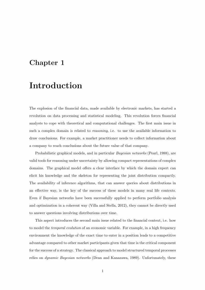
Chapter 1
Introduction
The explosion of the financial data, made available by electronic markets, has started a
revolution on data processing and statistical modeling. This revolution forces financial
analysts to cope with theoretical and computational challenges. The first main issue in
such a complex domain is related to reasoning, i.e. to use the available information to
draw conclusions. For example, a market practitioner needs to collect information about
a company to reach conclusions about the future value of that company.
Probabilistic graphical models, and in particular Bayesian networks (Pearl, 1988), are
valid tools for reasoning under uncertainty by allowing compact representations of complex
domains. The graphical model offers a clear interface by which the domain expert can
elicit his knowledge and the skeleton for representing the joint distribution compactly.
The availability of inference algorithms, that can answer queries about distributions in
an effective way, is the key of the success of these models in many real life contexts.
Even if Bayesian networks have been successfully applied to perform portfolio analysis
and optimization in a coherent way (Villa and Stella, 2012), they cannot be directly used
to answer questions involving distributions over time.
This aspect introduces the second main issue related to the financial context, i.e. how
to model the temporal evolution of an economic variable. For example, in a high frequency
environment the knowledge of the exact time to enter in a position leads to a competitive
advantage compared to other market participants given that time is the critical component
for the success of a strategy. The classical approach to model structured temporal processes
relies on dynamic Bayesian networks (Dean and Kanazawa, 1989). Unfortunately, these
1
1. Introduction
models suffer from two main drawbacks: the model instability related to the choice of the
discretization step and the computational burden related to inference. Continuous time
Bayesian networks (Nodelman et al., 2002) overcome the previous issues by modeling
time directly. These models are based both on homogeneous Markov processes, as they
model the transition dynamics of a system, and on Bayesian networks, as they provide
a graphical representation over a structured state space. These models can be used in
several financial contexts, such as for scenario generation based on historical data, for
the analysis of timing and probability related to securities, and for inferring the temporal
evolution of an economic variable when its state is not observed.
Two significant extensions of continuous time Bayesian networks have enhanced their
expressive power and usability. Firstly, continuous time Bayesian network classifiers
(Stella and Amer, 2012; Codecasa and Stella, 2014) allow to perform temporal classifi-
cation in continuous time. Specifically, in the case of complete data, they are effective for
performing inference and learning on a huge amount of data (Villa and Rossetti, 2014). In
finance, these classifiers can be used to exploit important features of high frequency data,
such as the unevenly spaced time data, and to perform the prediction of economic vari-
ables, such as the foreign exchange rate (Villa and Stella, 2014). Secondly, non-stationary
continuous time Bayesian networks allow to represent dependencies which change over
time (Stella and Villa, 2014). They can be used to analyze time-series data, such as
change-points detection, and reasoning about when and how these dependencies vary.
The third issue in finance is related to the decision-making modeling, i.e. how to
fruitfully exploit the previous models to make actionable decisions. For example, in the
context of trading, the problem is to choose the best action to perform in each possible
state of the market in order to maximize the portfolio return. Structured continuous time
Markov decision processes (Kan and Shelton, 2008) are a useful framework to represent
large and structured continuous time systems and they can be solved effectively using
approximate linear programming techniques. Unfortunately, this framework requires the
full knowledge of the environment, which is a rather strong assumption in finance. Model-
based reinforcement learning using structured continuous time Markov decision processes
relax this assumption allowing the decision-maker to learn the model from the interactions
with the unknown environment (Villa and Shelton, 2014a).
2
1. Introduction
1.1 Contributions
This thesis concerns probabilistic graphical models, specifically Bayesian networks, con-
tinuous time Bayesian networks and their extensions, for reasoning and decision-making
in finance. The contributions of this work can be summarized as follows:
• the interplay between modern portfolio theory and Bayesian networks has been ex-
ploited to propose a novel framework for portfolio analysis and optimization (Villa
and Stella, 2012). It allows the investor to easily incorporate his market’s views and
to select the optimal portfolio allocation based on that information;
• an algorithm for learning continuous time Bayesian network classifiers using the
MapReduce framework has been designed and developed (Villa and Rossetti, 2014).
It scales well in distributed environments and it is able to manage Big Data;
• the prediction of foreign exchange rates has been addressed as a classification problem
in which a continuous time Bayesian network classifier has been developed and used
to solve it (Villa and Stella, 2014). Empirical results show that these classifiers are
more effective and more efficient than dynamic Bayesian network classifiers;
• a definition of structurally non-stationary continuous time Bayesian networks has
been provided (Stella and Villa, 2014). The derivation of the Bayesian score, as well
as the learning algorithms, have been presented and developed. These models are
able to represent statistical dependencies that change over time;
• a model-based reinforcement learning algorithm to control structured continuous
time dynamic systems has been described and developed (Villa and Shelton, 2014a).
It efficiently manages the exploration-exploitation trade-off and it achieves a sample
efficiency which is logarithmic in the size of the problem description;
• an R package that leverages on the C++ engine of continuous time Bayesian networks
(Shelton et al., 2010) was designed and developed (Villa and Shelton, 2014b). It
provides a valid tool for rapid prototyping and analysis in the R environment;
• some path-breaking examples and insights about the use of continuous time Bayesian
networks and their extensions to tackle real financial problems are given.
3
1. Introduction
1.2 Overview
This thesis is organized in eight chapters according to the following structure:
• Chapter 2 presents an overview of the background elements about Bayesian net-
works, their representation ability, the learning algorithms and inference methods.
The last part of this chapter presents the interplay between modern portfolio theory
and Bayesian networks and how to exploit them in a new framework for portfolio
analysis and optimization;
• Chapter 3 covers the fundamental notions about continuous time Bayesian networks,
their semantics, the problem of parameter and structural learning from data, and
the issues of inference using such models. The last part of this chapter is devoted to
the discussion about the related models, such as dynamic Bayesian networks, and
the presentation of some financial applications;
• Chapter 4 treats the extension of continuous time Bayesian networks to solve the
problem of classification. It starts by introducing the basic concepts about temporal
classification, then it describes an efficient scalable learning algorithm for Big Data
and finally, it presents an application of continuous time Bayesian network classifiers
to the foreign exchange rate prediction problem in high frequency domain;
• Chapter 5 shows the extension of continuous time Bayesian networks to non-stationary
domains. After a brief discussion about the problem of learning in these domains, it
gives the formal definition of non-stationary continuous time Bayesian networks and
it presents the learning framework with three different structural learning settings
together with their corresponding learning algorithms. Finally, it provides numerical
experiments on synthetic data sets;
• Chapter 6 covers the basic notions about Markov decision processes used to model
sequential decision-making under uncertainty and it provides the main methods to
solve them. Then, it describes their extensions to represent large and structured
domains effectively using dynamic Bayesian networks. Finally, it shows how contin-
uous time Bayesian networks are used as basic models of structured continuous time
Markov decision processes with some examples in a structured trading domain;
4

1. Introduction
• Chapter 7 presents the background material about reinforcement learning with par-
ticular attention to the model-based reinforcement learning algorithms. After the
introduction on the use of factored Markov decision-making processes in the rein-
forcement learning environment, it presents a novel algorithm for control continuous
time dynamic systems based on structured continuous time Markov decision pro-
cesses. Finally, it provides numerical experiments on the trading domain, described
in the previous chapter, that demonstrate its effectiveness;
• Chapter 8 concludes the thesis with a brief summary and a discussion of future work.
5
Chapter 2
Bayesian networks
Bayesian networks are sound graphical models that encode probabilistic relationships
among random variables. We start this chapter by showing their representation abil-
ity, then describe how to perform learning. We move on review the inference methods,
then we finish by presenting the interplay between modern portfolio theory and Bayesian
networks and how to exploit them in a framework for portfolio analysis and optimization.
2.1 Representation
Bayesian networks are well developed frameworks used for many purposes, such as to model
and explain a domain, to update beliefs about states of certain variables when some other
variables are observed, to find most probable configurations of variables and to support
decision-making under uncertainty. We present the necessary background about Bayesian
networks, while we refer to Pearl (1988); Neapolitan (2003); Jensen and Nielsen (2007);
Koller and Friedman (2009) for further reference. One of the key aspects of Bayesian net-
works is the compact description of joint probability distributions. Assume that we would
like to represent a joint distribution over a set of N random variables X = {X1, . . . , XN}.
Even in the case of binary variables, the joint distribution requires the specification of the
probabilities of 2N assignments of the values x1, . . . , xN . Thus, this explicit representa-
tion is unmanageable even for small values of N . Bayesian networks overcome this issue
through the use of a factored representation which leverages on conditional independence.
6
2. Bayesian networks
2.1.1 Independence properties
The key idea of a factored representation is that, in a given domain, most variables do
not directly affect most other variables. Conversely, for each variable only a limited set
of other variables influences it. To illustrate this concept, we begin with the definition of
marginal independence for random variables.
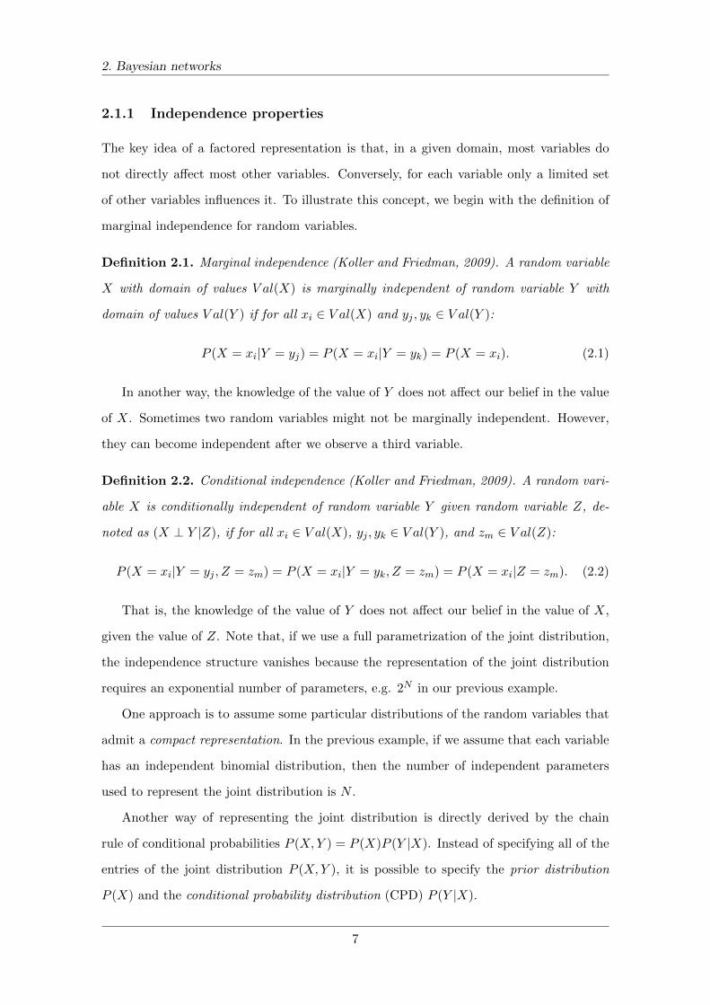
Definition 2.1. Marginal independence (Koller and Friedman, 2009). A random variable
X with domain of values V al(X) is marginally independent of random variable Y with
domain of values V al(Y ) if for all xi ∈ V al(X) and yj , yk ∈ V al(Y ):
P (X = xi|Y = yj) = P (X = xi|Y = yk) = P (X = xi). (2.1)
In another way, the knowledge of the value of Y does not affect our belief in the value
of X. Sometimes two random variables might not be marginally independent. However,
they can become independent after we observe a third variable.
Definition 2.2. Conditional independence (Koller and Friedman, 2009). A random vari-
able X is conditionally independent of random variable Y given random variable Z, de-
noted as (X ⊥ Y |Z), if for all xi ∈ V al(X), yj , yk ∈ V al(Y ), and zm ∈ V al(Z):
P (X = xi|Y = yj , Z = zm) = P (X = xi|Y = yk, Z = zm) = P (X = xi|Z = zm). (2.2)
That is, the knowledge of the value of Y does not affect our belief in the value of X,
given the value of Z. Note that, if we use a full parametrization of the joint distribution,
the independence structure vanishes because the representation of the joint distribution
requires an exponential number of parameters, e.g. 2N in our previous example.
One approach is to assume some particular distributions of the random variables that
admit a compact representation. In the previous example, if we assume that each variable
has an independent binomial distribution, then the number of independent parameters
used to represent the joint distribution is N .
Another way of representing the joint distribution is directly derived by the chain
rule of conditional probabilities P (X,Y ) = P (X)P (Y |X). Instead of specifying all of the
entries of the joint distribution P (X,Y ), it is possible to specify the prior distribution
P (X) and the conditional probability distribution (CPD) P (Y |X).
7
2. Bayesian networks
2.1.2 Definition
Bayesian networks effectively combine both qualitative and quantitative components. The
qualitative part consists in the graphical model that offers a clear interface by which the
domain expert can elicit his knowledge, while the quantitative part consists of potentials,
i.e. functions over sets of nodes of the graph. The graphical component of the Bayesian
network is specified as a directed acyclic graph (DAG) whose nodes are the random vari-
ables in the domain and edges correspond to direct influence of one node on another. This
graph compactly provides both the skeleton for representing the joint distribution and the
set of conditional independence assumptions about the distribution.
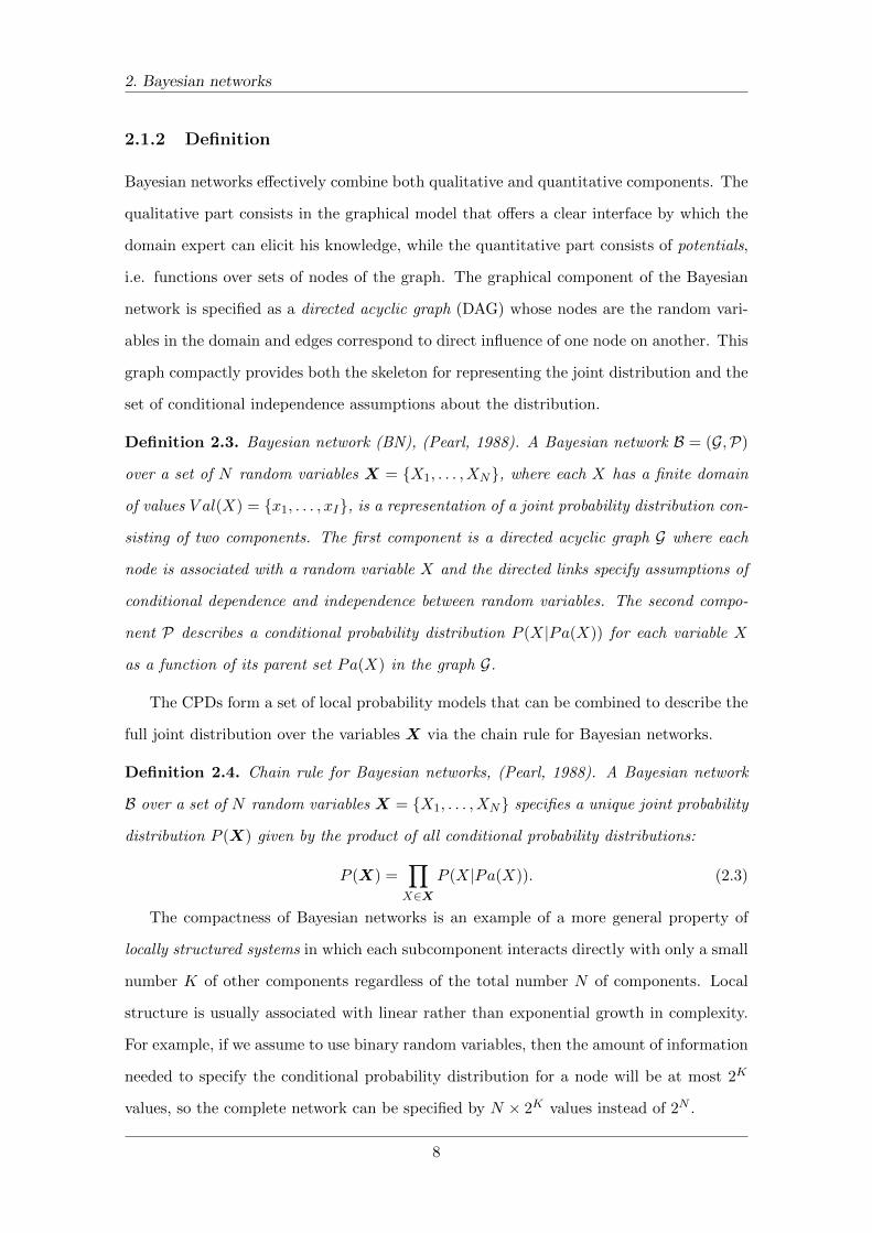
Definition 2.3. Bayesian network (BN), (Pearl, 1988). A Bayesian network B = (G,P)
over a set of N random variables X = {X1, . . . , XN}, where each X has a finite domain
of values V al(X) = {x1, . . . , xI}, is a representation of a joint probability distribution con-
sisting of two components. The first component is a directed acyclic graph G where each
node is associated with a random variable X and the directed links specify assumptions of
conditional dependence and independence between random variables. The second compo-
nent P describes a conditional probability distribution P (X|Pa(X)) for each variable X
as a function of its parent set Pa(X) in the graph G.
The CPDs form a set of local probability models that can be combined to describe the
full joint distribution over the variables X via the chain rule for Bayesian networks.
Definition 2.4. Chain rule for Bayesian networks, (Pearl, 1988). A Bayesian network
B over a set of N random variables X = {X1, . . . , XN} specifies a unique joint probability
distribution P (X) given by the product of all conditional probability distributions:
P (X) =∏X∈X
P (X|Pa(X)). (2.3)
The compactness of Bayesian networks is an example of a more general property of
locally structured systems in which each subcomponent interacts directly with only a small
number K of other components regardless of the total number N of components. Local
structure is usually associated with linear rather than exponential growth in complexity.
For example, if we assume to use binary random variables, then the amount of information
needed to specify the conditional probability distribution for a node will be at most 2K
values, so the complete network can be specified by N × 2K values instead of 2N .
8
2. Bayesian networks
2.1.3 Graph independencies
Dependencies and independencies are important properties of a distribution as they can
be exploited to substantially reduce the computational cost of inference. Indeed, BNs can
be used to assess how the change of certainty in one variable may change the certainty
for other variables. This certainty can be in the form of hard evidence if the variable is
instantiated, i.e. X = xi, or soft evidence otherwise. The graph structure G can be used
to extract independencies that hold for every distribution P that factorizes over G. A
fundamental property is called d-separation as it can be used for determining conditional
independencies: if two nodes X and Y are d-separated given node Z, then (X ⊥ Y |Z).
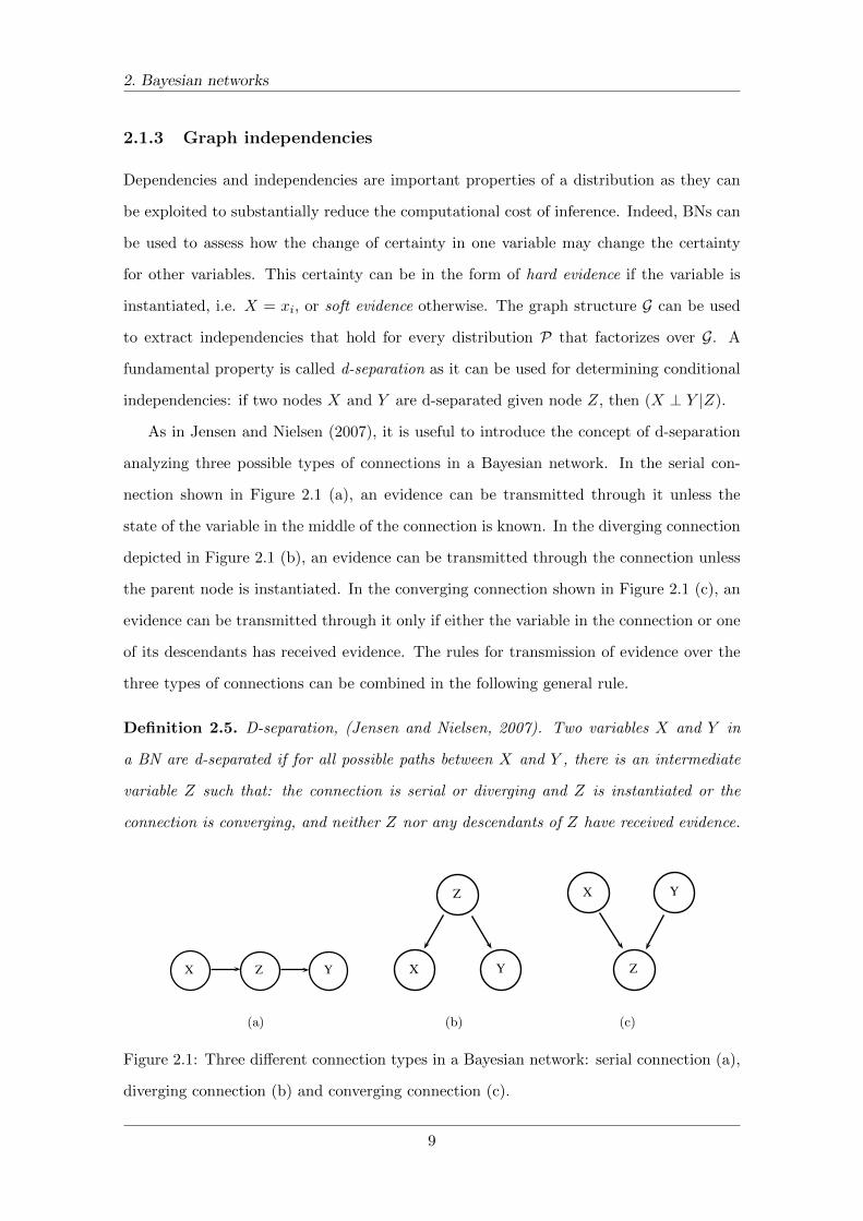
As in Jensen and Nielsen (2007), it is useful to introduce the concept of d-separation
analyzing three possible types of connections in a Bayesian network. In the serial con-
nection shown in Figure 2.1 (a), an evidence can be transmitted through it unless the
state of the variable in the middle of the connection is known. In the diverging connection
depicted in Figure 2.1 (b), an evidence can be transmitted through the connection unless
the parent node is instantiated. In the converging connection shown in Figure 2.1 (c), an
evidence can be transmitted through it only if either the variable in the connection or one
of its descendants has received evidence. The rules for transmission of evidence over the
three types of connections can be combined in the following general rule.
Definition 2.5. D-separation, (Jensen and Nielsen, 2007). Two variables X and Y in
a BN are d-separated if for all possible paths between X and Y , there is an intermediate
variable Z such that: the connection is serial or diverging and Z is instantiated or the
connection is converging, and neither Z nor any descendants of Z have received evidence.
X YZ
(a)
X Y
Z
(b)
X Y
Z
(c)
Figure 2.1: Three different connection types in a Bayesian network: serial connection (a),
diverging connection (b) and converging connection (c).
9

2. Bayesian networks
From the definition of d-separation, we can introduce the concept of Markov blanket of
a node X. This notion is important because when the Markov blanket of X is instantiated,
X becomes d-separated from the rest of the network.
Definition 2.6. Markov blanket, (Pearl, 1988). The Markov blanket of a variable X in
a Bayesian network is the set consisting of the parents of X, the children of X and the
variables sharing a child with X.
Finally, we mention two useful structures to derive independence statements in a
Bayesian network. Firstly, the moral graph of a Bayesian network: it is an undirected
graph obtained by adding an edge between any two nodes that share a common child in
the DAG of the BN and then by dropping the directionality of all edges. The moral graph
can be used to check whether X and Y are d-separated given Z. In fact, if all paths
connecting X and Y intersect Z, then X and Y are d-separated given Z (Jensen and
Nielsen, 2007). Secondly, the jointree of a Bayesian network: it is a tree of clusters where
each cluster is a set of variables in the Bayesian network sharing two properties. The first
one states that every node and its parents must appear in some cluster and the second one
states that if a variable appears in two clusters, then it must also appear in every cluster
on the path between them. The jointree of a BN can be used to check whether two sets
of variables are independent. In fact, any two clusters are independent given any cluster
on the path connecting them (Pearl, 1988).
X Y
Z
W V
(a)
X Y
Z
W V
(b)
X,Y,Z Y,V
X,Y,W
(c)
Figure 2.2: A Bayesian network (a), the corresponding moral graph (b) and a jointree (c).
10
2. Bayesian networks
2.2 Learning
Bayesian networks can be learned directly from data. In particular, if we assume that the
domain is governed by some underlying distribution and we have a data set of samples
from it, then the goal of learning is to construct a BN that captures the original underlying
distribution in the best possible way. There are different reasons to learn a BN, such as to
perform inference, to solve a classification task and to knowledge discovery, i.e. to reveal
some important properties of the domain.
We discuss about the basic notions of parameter and structural learning. Parameter
learning is concerned with the estimation of the elements of the CPDs when the graph
is known, while structural learning is concerned with the selection of the graph and the
estimation of the CPDs. Parametric and structural learning can be developed for complete
data or missing data arising from partial observability of the random variables. We cover
the first case, while we refer to Koller and Friedman (2009) for the second case.
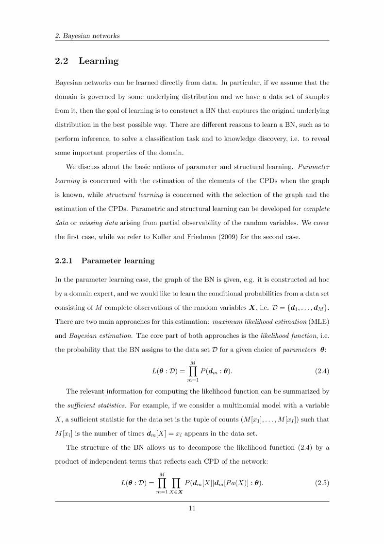
2.2.1 Parameter learning
In the parameter learning case, the graph of the BN is given, e.g. it is constructed ad hoc
by a domain expert, and we would like to learn the conditional probabilities from a data set
consisting of M complete observations of the random variables X, i.e. D = {d1, . . . ,dM}.
There are two main approaches for this estimation: maximum likelihood estimation (MLE)
and Bayesian estimation. The core part of both approaches is the likelihood function, i.e.
the probability that the BN assigns to the data set D for a given choice of parameters θ:
L(θ : D) =M∏m=1
P (dm : θ). (2.4)
The relevant information for computing the likelihood function can be summarized by
the sufficient statistics. For example, if we consider a multinomial model with a variable
X, a sufficient statistic for the data set is the tuple of counts (M [x1], . . . ,M [xI ]) such that
M [xi] is the number of times dm[X] = xi appears in the data set.
The structure of the BN allows us to decompose the likelihood function (2.4) by a
product of independent terms that reflects each CPD of the network:
L(θ : D) =
M∏m=1
∏X∈X
P (dm[X]|dm[Pa(X)] : θ). (2.5)
11
2. Bayesian networks
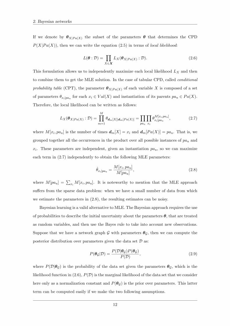
If we denote by θX|Pa(X) the subset of the parameters θ that determines the CPD
P (X|Pa(X)), then we can write the equation (2.5) in terms of local likelihood:
L(θ : D) =∏X∈X
LX(θX|Pa(X) : D). (2.6)
This formulation allows us to independently maximize each local likelihood LX and then
to combine them to get the MLE solution. In the case of tabular CPD, called conditional
probability table (CPT), the parameter θX|Pa(X) of each variable X is composed of a set
of parameters θxi|pau for each xi ∈ V al(X) and instantiation of its parents pau ∈ Pa(X).
Therefore, the local likelihood can be written as follows:
LX(θX|Pa(X) : D) =
M∏m=1
θdm[X]|dm[Pa(X)] =∏pau
∏xi
θM [xi,pau]xi|pau , (2.7)
where M [xi, pau] is the number of times dm[X] = xi and dm[Pa(X)] = pau. That is, we
grouped together all the occurrences in the product over all possible instances of pau and
xi. These parameters are independent, given an instantiation pau, so we can maximize
each term in (2.7) independently to obtain the following MLE parameters:
θxi|pau =M [xi, pau]
M [pau], (2.8)
where M [pau] =∑
xiM [xi, pau]. It is noteworthy to mention that the MLE approach
suffers from the sparse data problem: when we have a small number of data from which
we estimate the parameters in (2.8), the resulting estimates can be noisy.
Bayesian learning is a valid alternative to MLE. The Bayesian approach requires the use
of probabilities to describe the initial uncertainty about the parameters θ, that are treated
as random variables, and then use the Bayes rule to take into account new observations.
Suppose that we have a network graph G with parameters θG , then we can compute the
posterior distribution over parameters given the data set D as:
P (θG |D) =P (D|θG)P (θG)
P (D), (2.9)
where P (D|θG) is the probability of the data set given the parameters θG , which is the
likelihood function in (2.6), P (D) is the marginal likelihood of the data set that we consider
here only as a normalization constant and P (θG) is the prior over parameters. This latter
term can be computed easily if we make the two following assumptions.
12
2. Bayesian networks
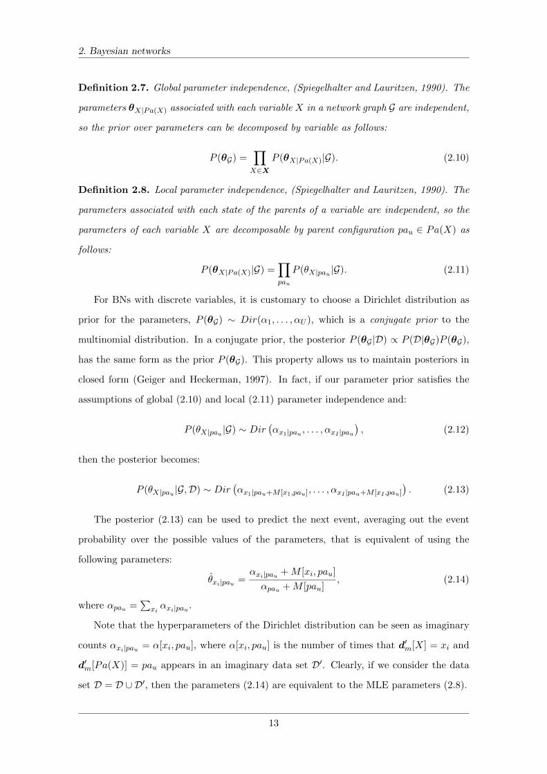
Definition 2.7. Global parameter independence, (Spiegelhalter and Lauritzen, 1990). The
parameters θX|Pa(X) associated with each variable X in a network graph G are independent,
so the prior over parameters can be decomposed by variable as follows:
P (θG) =∏X∈X
P (θX|Pa(X)|G). (2.10)
Definition 2.8. Local parameter independence, (Spiegelhalter and Lauritzen, 1990). The
parameters associated with each state of the parents of a variable are independent, so the
parameters of each variable X are decomposable by parent configuration pau ∈ Pa(X) as
follows:
P (θX|Pa(X)|G) =∏pau
P (θX|pau |G). (2.11)
For BNs with discrete variables, it is customary to choose a Dirichlet distribution as
prior for the parameters, P (θG) ∼ Dir(α1, . . . , αU ), which is a conjugate prior to the
multinomial distribution. In a conjugate prior, the posterior P (θG |D) ∝ P (D|θG)P (θG),
has the same form as the prior P (θG). This property allows us to maintain posteriors in
closed form (Geiger and Heckerman, 1997). In fact, if our parameter prior satisfies the
assumptions of global (2.10) and local (2.11) parameter independence and:
P (θX|pau |G) ∼ Dir(αx1|pau , . . . , αxI |pau
), (2.12)
then the posterior becomes:
P (θX|pau |G,D) ∼ Dir(αx1|pau+M [x1,pau], . . . , αxI |pau+M [xI ,pau]
). (2.13)
The posterior (2.13) can be used to predict the next event, averaging out the event
probability over the possible values of the parameters, that is equivalent of using the
following parameters:
θxi|pau =αxi|pau +M [xi, pau]
αpau +M [pau], (2.14)
where αpau =∑
xiαxi|pau .
Note that the hyperparameters of the Dirichlet distribution can be seen as imaginary
counts αxi|pau = α[xi, pau], where α[xi, pau] is the number of times that d′m[X] = xi and
d′m[Pa(X)] = pau appears in an imaginary data set D′. Clearly, if we consider the data
set D = D ∪D′, then the parameters (2.14) are equivalent to the MLE parameters (2.8).
13
2. Bayesian networks
2.2.2 Structural learning
Eliciting Bayesian networks from experts can be a laborious task in non trivial networks
(Mascherini and Stefanini, 2007). In the case where the network structure in unknown,
our goal is to reconstruct it from data. Unfortunately, since the space of all possible BNs
is combinatorial, finding the optimal one is NP-hard in the general case (Chickering et al.,
1994). However, some methods can be used to solve this task in an approximate way.
One approach is to consider a BN as a representation of independencies and to perform
conditional dependency and independency tests in the data in order to find an equivalence
class of networks that best explains these relationships. This approach, called constraint-
based structural learning, is quite intuitive, but it can be very sensitive to failures in
individual independence tests (Verma and Pearl, 1992; Cheng et al., 2002).
Another approach is to view a BN as a statistical model and then to address learning
as a model selection problem. This approach, called score-based structural learning, defines
a set of potential structures, a scoring function that measures how well the model fits the
data, and a search technique that finds the highest-scoring structure (Spiegelhalter et al.,
1993). We discuss this latter approach where the score is represented from a Bayesian
perspective. This is similar to what we have presented in the Bayesian parameter learning,
but in this context the uncertainty is both over structure and over parameters.
Once we have defined a structure prior P (G), that puts a prior probability on different
graphs, and a parameter prior P (θG |G), that puts a probability on different choice of
parameters given the graph, we can use the Bayes rule to compute P (G|D) as follows:
P (G|D) =P (D|G)P (G)
P (D). (2.15)
Given that the marginal likelihood of the data does not help us to distinguish between
different graphs, we define the Bayesian score BS as the logarithm of the numerator in
equation (2.15) as follows:
BS(G : D) = lnP (G) + lnP (D|G). (2.16)
The first term in (2.16) is the prior over structures that gives us a way of preferring
some structures over others in the first stages. However, as it does not grow with the size
of the data, a simple prior such as a uniform is often chosen. A key property of this prior
is that it must satisfy structure modularity.
14
2. Bayesian networks
Definition 2.9. Structure modularity, (Friedman and Koller, 2000). The prior over
structure P (G) decomposes into a product with a term for each variable in the domain:
P (G) =∏X∈X
P (Pa(X) = PaG(X)). (2.17)
The second term in (2.16) is the marginal likelihood of the data given the structure
and it is computed by marginalizing out the unknown parameters as follows:
P (D|G) =
∫θG
P (D|θG ,G)P (θG |G)dθG , (2.18)
where P (D|θG ,G) is the likelihood of the data given the graph structure G and its param-
eters θG , while P (θG |G) is the prior over parameters. In structural learning, this prior
over parameters is required to satisfy parameter modularity.
Definition 2.10. Parameter modularity, (Geiger and Heckerman, 1997). If a node X has
the same parents in two distinct graphs G and G′, PaG(X) = PaG′(X), then the probability
density functions of the parameters associated with this node must be identical:
P (θX|PaG(X)|G) = P (θX|PaG′ (X)|G′). (2.19)
In the case of complete data, P (D|G) can be computed in closed form by using the
Bayesian-Dirichlet equivalent (BDe) metric (Heckerman et al., 1995). It assumes that
P (θG |G) satisfies global (2.10) and local (2.11) parameter independence, parameter mod-
ularity (2.19) and Dirichlet prior (2.12). So, P (D|G) can be written as follows:
P (D|G) =∏X∈X
∏pau
Γ (αpau)
Γ (αpau +M [pau])×∏xi
Γ(αxi|pau +M [xi, pau]
)Γ(αxi|pau
) . (2.20)
If we set αxi|pau = α|xi|×|pau| , then the parameter priors are all controlled by a single
hyperparameter α. In this case, formula (2.20) becomes a uniform BDe (BDeu) metric.
If the network structure is in the form of tree or we have an ordering over variables,
then the search for the optimal structure can be performed polynomially in number of
variables (given a fixed number of possible parents for a node). In all other cases, we have
to determine how to move through the space of all networks, e.g. with operators of add,
delete or reverse an edge (Giudici and Castelo, 2003), and resort to heuristics or sampling
strategies for search procedures (Madigan et al., 1995; Chickering et al., 1995).
15
2. Bayesian networks
2.3 Inference
Since a BN defines a joint distribution over variables, it can be used to answer any prob-
abilistic query. For example, we can compute P (Y |E = e), where Y ,E ⊆X and e is an
instantiation of E, dividing P (Y , e) by P (e). Specifically, each of the instantiations of
P (Y , e) is a probability P (y, e) which can be computed by summing out all entries in the
joint that correspond to assignments consistent with (y, e), i.e. P (y, e) =∑z P (y, e, z),
where the set Z = X \{Y ,E} and P (e) can be computed directly as P (e) =∑y P (y, e).
However, this approach of compute the joint distribution and exhaustively sum out the
joint is not efficient, as we incur in the exponential blowup of the inference task. Even if
the problem of inference in graphical models is NP-hard (Cooper, 1990), many real-world
applications can be tackled effectively using exact or approximate inference algorithms.
2.3.1 Exact inference
The variable elimination algorithm (Shachter et al., 1990; Dechter, 1999) addresses the
exponential blowup of inference by computing the expressions in the joint distribution that
depend on a small number of variables once and by caching the results. The key concept
of this algorithm will be useful in the next chapters. As in Koller and Friedman (2009),
we use the notion of factor φ with Scope[φ] = Y , which is a function φ : V al(Y )→ R.
The basic operation is the factor marginalization. Let Y ⊆ X, Z ∈ X \ Y and
φ(Y , Z) a factor, the factor marginalization of Z in φ is another factor ψ over Y such that
ψ(Y ) =∑
Z φ(Y , Z). We observe that the operations of factor product and summation
behave precisely as do product and summation over numbers, specifically, ifX /∈ Scope[φ1],
then we can exchange summation and product easily as∑
X(φ1 × φ2) = φ1 ×∑
X φ2.
For example, if we assume to have a simple BN of four variables, specified as a serial
connection, X1 → X2 → X3 → X4, then the marginal distribution over X4 is:
P (X4) =∑X3
∑X2
∑X1
P (X1, X2, X3, X4) (2.21)
=∑X3
∑X2
∑X1
φ(X1)× φ(X2)× φ(X3)× φ(X4) (2.22)
=∑X3
φ(X4)× (∑X2
φ(X3)× (∑X1
φ(X2)φ(X1))). (2.23)
These different transformations are justified by the limited scope of each factor.
16
2. Bayesian networks
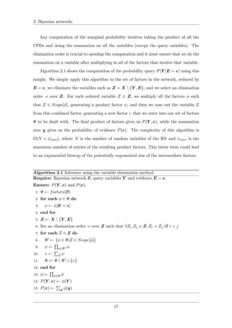
Any computation of the marginal probability involves taking the product of all the
CPDs and doing the summation on all the variables (except the query variables). The
elimination order is crucial to speedup the computation and it must ensure that we do the
summation on a variable after multiplying in all of the factors that involve that variable.
Algorithm 2.1 shows the computation of the probability query P (Y |E = e) using this
insight. We simply apply this algorithm to the set of factors in the network, reduced by
E = e, we eliminate the variables such as Z = X \ {Y ,E}, and we select an elimination
order ≺ over Z. For each ordered variable Z ∈ Z, we multiply all the factors φ such
that Z ∈ Scope[φ], generating a product factor ψ, and then we sum out the variable Z
from this combined factor, generating a new factor υ that we enter into our set of factors
Φ to be dealt with. The final product of factors gives us P (Y , e), while the summation
over y gives us the probability of evidence P (e). The complexity of this algorithm is
O(N × ψmax), where N is the number of random variables of the BN and ψmax is the
maximum number of entries of the resulting product factors. This latter term could lead
to an exponential blowup of the potentially exponential size of the intermediate factors.
Algorithm 2.1 Inference using the variable elimination method
Require: Bayesian network B, query variables Y and evidence E = e.
Ensure: P (Y , e) and P (e).
1: Φ← factors(B)
2: for each φ ∈ Φ do
3: φ← φ[E = e]
4: end for
5: Z ←X \ {Y ,E}6: Set an elimination order ≺ over Z such that ∀Zi, Zj ∈ Z, Zi ≺ Zj iff i < j
7: for each Z ∈ Z do
8: Φ′ ← {φ ∈ Φ|Z ∈ Scope[φ]}9: ψ ←∏
φ∈Φ′ φ
10: υ ←∑Z ψ
11: Φ← Φ \ Φ′ ∪ {υ}12: end for
13: φ←∏φ∈Φ φ
14: P (Y , e)← φ(Y )
15: P (e)←∑y φ(y)
17
2. Bayesian networks
We can think the elimination steps 7 - 12 of Algorithm 2.1 as a sequence of graph
manipulations induced by the set of factors Φ. Specifically, we have an undirected graph
whose nodes correspond to the variables in the Scope[Φ] and edges (X,Y ) iff there exists
a factor φ ∈ Φ : X,Y ∈ Scope[φ]. Step 9 generates edges between all the variables with
which Z appears in factors, while step 10 has the effect of removing Z and all of its incident
edges from the graph. Every factor that appears in one of the elimination steps is reflected
in the graph as a clique. Consider the induced graph as the union of the graphs resulting
in all the elimination steps, given an elimination order; then its width is the number of
nodes in the largest clique minus one, and the tree-width is the minimal induced width.
The tree-width gives us a bound on the performance of Algorithm 2.1 that depends on
the elimination order. Finding the optimal order is NP-hard (Arnborg et al., 1987), but
some heuristics have been proposed (Reed, 1992; Becker and Geiger, 2001).
An alternative approach is tree clustering, which is also known as the jointree algorithm
(Lauritzen and Spiegelhalter, 1988; Jensen et al., 1990). The key idea is to organize the
set of factors into a jointree and then use this structure to control the process of variable
elimination. A third approach of exact inference is based on the concept of conditioning
(Pearl, 1986; Horvitz et al., 1989; Darwiche, 1995). The key idea is that if we know the
value of a variable X, then we can remove edges outgoing from X, modify the CPTs for
children of X and then perform inference on the simplified network.
2.3.2 Approximate inference
Exact inference become infeasible for BNs with large tree-width, indeed the computational
and space complexity of the clique tree is exponential in the tree-width of the network.
We review some approximate inference methods in which the joint distribution is approx-
imated by a set of instantiations to some of the variables in the network, called particles.
The simplest approach to generate particles is forward sampling. Given M random
samples D = {d1, . . . ,dM} from the distribution P (X), forward sampling estimates the
expectation of a target function as empirical mean over samples. If we want to compute
P (y), then its estimate is the fraction of particles where we have seen the event y:
P (y) =1
M
M∑m=1
1{y}(dm[Y ]), (2.24)
18
2. Bayesian networks
where 1 is the indicator function and dm[Y ] is the value of variables Y in the sample dm.
In the case where we are interested in conditional probabilities P (y|e), one approach
is to generate samples directly from the posterior P (X|e) using a method called rejection
sampling. In practice, it generates samples from P (X) as in the previous case, but it
rejects any sample that is not compatible with e. The problem is that the number of
rejected particles can be huge, i.e. proportional to M × P (e).
Another approach is importance sampling, a general procedure for estimating the ex-
pectation of a function relative to a target distribution from a different distribution, called
proposal distribution, which is much more simple to sample. In the context of BNs, a sim-
ple proposal distribution can be described in terms of a Bayesian network. Specifically,
let B be a BN and y an instantiation of Y , then the proposal distribution By is the same
as B except that each node Y ∈ Y has no parents and its CPD gives probability 1 to
Y = y and 0 to all other values. The sampling process is similar to forward sampling, but
we have weighted particles, i.e. for each sample d′ coming from the proposal distribution
we have its weight w(d′). This weight can be derived from the likelihood of the evidence
accumulated throughout the sampling process:
w(d′) =PB(d′)
PBy(d′)=∏X∈Y
LX(θX|Pa(X) : d′m) =∏X∈Y
θd′m[X]|d′m[Pa(X)]. (2.25)
Therefore, the weight w(d′) is the likelihood contribution of all the variables in Y ; this
approach is also know as likelihood weighting (Shachter and Peot, 1989). An estimate of
P (y) can performed using (unnormalized) importance sampling as follows:
P (y) =1
M ′
M ′∑m=1
1{y}(d′m[Y ])w(d′m), (2.26)
while an estimate of P (y|e) for a given event e can be computed in two steps. We generate
M ′′ weighted particles from a proposal distribution defined by By,e and M ′ weighted
particles from a proposal distribution defined by Be, then we compute the following ratio:
P (y|e) =M ′
M ′′
∑M ′′
m=1 1{y,e}(d′′m[Y,E])w(d′′m)∑M ′
m=1 1{e}(d′m[E])w(d′m)
. (2.27)
Note that the quality of importance sampling depends largely on how close the proposal
distribution is to the target distribution. In fact, if the proposal is very different from the
target distribution, then most of the samples will be irrelevant, i.e. with a low weight.
19
2. Bayesian networks
2.4 BNs for portfolio analysis and optimization
Bayesian networks have been widely used in many contexts, such as medicine (Andreassen
et al., 1987; Luciani et al., 2003; Lucas et al., 2004), computer science (de Campos et al.,
2004; Fagiuoli et al., 2008) and finance (Demirer et al., 2006; Pavlenko and Chernyak, 2010;
Rebonato and Denev, 2014). The range of applications is very wide and demonstrates the
extensive applicability of Bayesian networks in real life domains.
In this section we present how to exploit the interplay between modern portfolio theory
and Bayesian networks to describe the framework for portfolio analysis and optimization
introduced by Villa and Stella (2012). This framework leverages on evidential reasoning
to understand the behavior of an investment portfolio in different economic and finan-
cial scenarios. It allows to formulate and solve a portfolio optimization problem, while
coherently taking into account the investor’s market views. Some examples of portfolio
analysis and optimization on the DJ Euro Stoxx 50 Index, exploiting evidential reasoning
on Bayesian networks, are presented and discussed.
2.4.1 Financial context
Portfolio analysis and portfolio optimization are basic problems in computational finance.
They have been intensively studied over the last sixty years and several relevant contribu-
tions are available in the specialized literature (Elton et al., 2010). Portfolio optimization
originates from the seminal paper of Markowitz (1952) who introduced the mean-variance
investment framework, the first quantitative treatment of the risk-return trade-off. This
conventional approach to portfolio optimization consists of two steps. The first one con-
cerns distributional assumptions about the behavior of stock prices, while the second one
is related to the selection of the optimal portfolio, depending on some objective func-
tion and/or utility function, defined according to the investor’s goal. This conceptual
model in the past proved to be useful even if many drawbacks have been pointed out
by finance practitioners, private investors and researchers. The basic formulation intro-
duced by Markowitz has been extended in the specialized literature by taking into account
additional moments of the portfolio’s return distribution and by developing necessary con-
ditions on the utility function of investors (Fabozzi et al., 2007).
20
2. Bayesian networks
It is increasingly understood that the investor’s experience, i.e. his qualitative and
quantitative knowledge on economy, finance and financial markets, is a key factor for
success. Indeed, the knowledge of some factors, such as the likelihood of future events,
the outlook on finance and economy, the coexistence of different asset pricing theories and
the security-driving forces, can be fruitfully exploited to formulate and solve the portfolio
optimization problem. The first contribution that exploits investor’s market views in a
quantitative way is due to Black and Litterman (1991). In their work, they tried to
overcome some typical problems of mean-variance investment framework, such as the lack
of diversification and instabilities of portfolios on the efficient frontier, by using a Bayesian
approach that combines the investor’s market views about the expected returns of some
assets with those of the market equilibrium defined by the capital asset pricing model of
Sharpe (1964). Unfortunately, the building of the required inputs is somewhat complex and
not intuitive for an investor without quantitative background. Different improvements and
extensions of this model have been developed, such as conditional-marginal factorization
used to input views on volatilities, correlations and expectations (Qian and Gorman, 2001),
the use of market views without any preprocessing (Meucci, 2006) and the use of market
views directly on on the risk factors underlying the market instead of the returns of the
securities (Meucci, 2009).
2.4.2 Basics of portfolio modeling and optimization
The goal of the portfolio modeling task consists of forecasting and managing the portfolio’s
profit and loss distribution at the investment horizon. In order to describe this task, we
assume to have N securities, a sequence of N -dimensional vectors of spot prices St indexed
by time t sampled at time interval ∆t, T is the time when the portfolio allocation decision
has to be made and τ is the investment horizon. The portfolio modeling task can be
accomplished in the following steps according to Meucci (2011).
The first step consists of the identification of the risk drivers. A risk driver of a
security is modeled with a random variable X, sharing the following two properties: it
fully specifies the price of the security at time t and it follows a homogeneous stochastic
process. Once the risk drivers have been identified, we have to extract the invariants from
them. An invariant is a shock that steers the stochastic process associated with the risk
21
2. Bayesian networks
driver. The risk driver can be modeled by a set of independent and identically distributed
random variables, and it becomes known at time t + ∆t. To connect the invariant Yt to
the risk driver Xt at time t, we use the following relation:
Yt = h(Xt)− h(Xt−∆t), (2.28)
where h is an invertible deterministic function. For example, the risk driver of a stock is
the natural logarithm of its price, while the relative invariant is the compounded return.
The second step concerns the estimation of the distribution of the invariants which
does not depend on the specific time t because of the invariance property. This task
can be accomplished by fitting an empirical distribution from the invariants time-series
through multivariate statistical techniques, such as simple historical, maximum likelihood
and robust, see Meucci (2005) for an in-depth overview. A dimension reduction technique
is fundamental to reduce the number of invariants, such as a linear factor model that
decomposes the J-dimensional invariants Y t as follows:
Y t = BtF t +U t, (2.29)
where F t is an M -dimensional vector of factors with M � J ,Bt is a J×M matrix of factor
loadings which links the factors F t to the invariants Y t, while U t is a J-dimensional vector
of residuals. These factors can be used to synthesize the entire invariants’ distribution.
The third step consists of the projection of the invariants’ distribution to the investment
horizon τ . This projection can be implemented in different ways. If the risk drivers evolve
according to a random walk, then the first two moments of the projected distribution can
be obtained through recursion (Meucci, 2005), while the projection of the full distribution
can be accomplished by the Fourier transform techniques (Albanese et al., 2004).
The fourth step is the pricing of the securities at investment horizon τ :
Sτ = g(Xτ , tc), (2.30)
where g is the pricing function, the risk drivers Xτ are extracted from the projected
invariants’ distribution and tc are the terms and conditions of the securities.
The last step involves the computation of the profit and loss distribution at investment
horizon Aτ given a portfolio with holdings a = (a1, . . . , aN ) as follows:
Aτ = a′(Sτ − ST ). (2.31)
22
2. Bayesian networks
Once we have estimated the prices at the investment horizon, we can optimize our
portfolio using the standard mean-variance portfolio optimization framework. When the
investor’s objective is the terminal wealth and the initial capital is non-null, the portfolio
optimization problem can be formulated in terms of a vector of linear returns at investment
horizon Lτ and a vector of weights w as follows:
w∗υ = argmaxw∈Λ,
w′Cov[Lτ ]w=υ,
{w′E[Lτ ]
}, (2.32)
where E[Lτ ] and Cov[Lτ ] are, respectively, expected value and covariance matrix of linear
returns at investment horizon, while υ is the desired level of risk and Λ is the set of
constraints. If a budget constraint is introduced (w′1 = 1) and short-selling is not allowed
(w ≥ 0), then the optimization problem is quadratic and thus can be solved analytically.
2.4.3 The integrated perspective
The portfolio modeling and optimization tasks can be seen in an integrated perspective.
The goal is to preserve the joint probability distribution of the factors and the invariants,
as it allows us to perform evidential reasoning on some selected factors; this distribution
should be factored properly to avoid the exponential blowup of the full representation. A
straightforward way to perform this is to construct a Bayesian network that relates factors
to invariants, from the latter it is possible to determine the risk drivers and the prices (or
returns) of securities and then to obtain the portfolio distribution from aggregation.
We can think the implementation of this process as a three-layered model. The first is
a Bayesian network layer that links the key factors with the invariants, while providing a
compact description of the market. This layer can be used to perform efficient evidential
reasoning. In fact, we can introduce evidences concerning the nodes associated with the
factors and then obtain the posterior probability over the nodes associates with invariants.
The second is a transformation layer that deterministically links the invariants to the risk
drivers and prices. This layer is useful because, in general, we are not only interested in
analyzing the posterior distribution of the invariants, but rather the distribution of the
risk drivers, prices and returns. The last one is an aggregation layer that represents the
portfolio’s securities. This layer links the market securities with those that we have in
portfolio, allowing us to perform portfolio analysis and optimization with the given views.
23
2. Bayesian networks
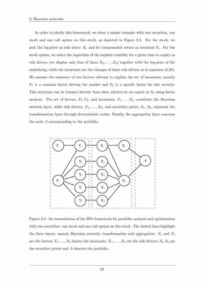
In order to clarify this framework, we show a simple example with two securities, one
stock and one call option on this stock, as depicted in Figure 2.3. For the stock, we
pick the log-price as risk driver X1 and its compounded return as invariant Y1. For the
stock option, we select the logarithm of the implied volatility for a given time to expiry as
risk drivers (we display only four of them X2, . . . , X4) together with the log-price of the
underlying, while the invariants are the changes of these risk drivers as in equation (2.28).
We assume the existence of two factors relevant to explain the set of invariants, namely
F1 is a common factor driving the market and F2 is a specific factor for this security.
This structure can be learned directly from data, elicited by an expert or by using factor
analysis. The set of factors, F1, F2, and invariants, Y1, . . . , Y5, constitute the Bayesian
network layer, while risk drivers, X1, . . . , X5, and securities prices, S1, S2, represent the
transformation layer through deterministic nodes. Finally, the aggregation layer concerns
the node A corresponding to the portfolio.
Y1
Y2
F1
F2
Y3
Y4
Y5
X 1
X 2
X 3
X 4
X 5
S1
S 2
A
Figure 2.3: An instantiation of the BNs framework for portfolio analysis and optimization
with two securities: one stock and one call option on this stock. The dotted lines highlight
the three layers, namely Bayesian network, transformation and aggregation. F1 and F2
are the factors, Y1, . . . , Y5 denote the invariants, X1, . . . , X5 are the risk drivers, S1, S2 are
the securities prices and A denotes the portfolio.
24
2. Bayesian networks
2.4.4 Case study
Villa and Stella (2012) presented a case study about an equity investor interested in
analyzing, stress testing and optimizing the tomorrow’s return distribution of his portfolio.
The eligible universe was the Eurozone Blue-chips forming the DJ Euro Stoxx 50 Index
and the available data set consisted of five years of daily prices, spanning from December
30th, 2005, to December 30th, 2010. Note that the basic steps of portfolio modeling are
more easily compared to the general case because the risk drivers are the log-prices, the
pricing function is the exponential function and it is not needed to project the invariant
distribution because of the estimation interval is equal to the investment horizon. So, it is
possible to focus only on the estimation of the invariants’ distribution and the identification
of the underlying factors. The authors have shown how the standard quantitative approach
to portfolio analysis and optimization can be seen as an instantiation of the proposed
framework and how it can be used to enrich the analysis with investor’s market views.
As first case, a statistical factor model based on random matrix theory and Monte
Carlo simulation with normal copula have been used to generate a panel of 100,000 joint
scenarios from the data set (Meucci, 2010). Factor analysis using random matrix theory
allows to model the invariants with M � J informative factors plus a residual term
represented by J −M noise factors (Plerou et al., 2002). The M = 10 largest eigenvalues
of the empirical covariance matrix have been used. The framework has been instantiated
as follows. The BN layer was constructed by discretizing these estimation factors into
three states (low, medium and high), the invariants into one hundred states and then
using MLE for learning the parameters of a fully connected network. The transformation
layer deterministically linked the invariants to the risk drivers and then to the securities’
returns; finally the portfolio was determined by aggregation of securities’ returns.
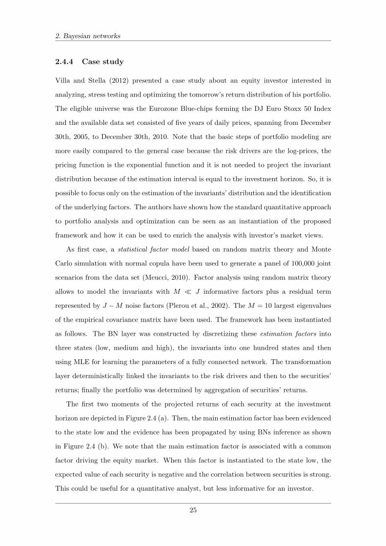
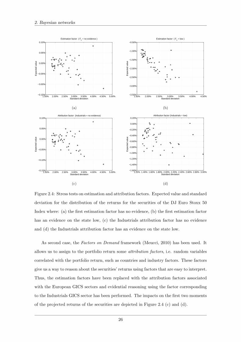
The first two moments of the projected returns of each security at the investment
horizon are depicted in Figure 2.4 (a). Then, the main estimation factor has been evidenced
to the state low and the evidence has been propagated by using BNs inference as shown
in Figure 2.4 (b). We note that the main estimation factor is associated with a common
factor driving the equity market. When this factor is instantiated to the state low, the
expected value of each security is negative and the correlation between securities is strong.
This could be useful for a quantitative analyst, but less informative for an investor.
25
2. Bayesian networks
1.50% 2.00% 2.50% 3.00% 3.50% 4.00% 4.50% 5.00%−0.15%
−3.00%
−0.05%
0.00%
0.05%
0.10%
Estimation factor ( F1 = no evidence )
Standard deviation
Exp
ecte
d va
lue
(a)
1.50% 2.00% 2.50% 3.00% 3.50% 4.00% 4.50%−3.50%
−3.00%
−2.50%
−2.00%
−1.50%
−1.00%
−0.50%
Estimation factor ( F1 = low )
Standard deviation
Exp
ecte
d va
lue
(b)
1.50% 2.00% 2.50% 3.00% 3.50% 4.00% 4.50% 5.00%−0.15%
−0.10%
−0.05%
0.00%
0.05%
0.10%Attribution factor (Industrials = no evidence)
Standard deviation
Exp
ecte
d va
lue
(c)
1.20% 1.40% 1.60% 1.80% 2.00% 2.20% 2.40% 2.60% 2.80% 3.00%−1.60%
−1.40%
−1.20%
−1.00%
−0.80%
−0.60%
−0.40%
−0.20%
0.00%
0.20%Attribution factor (Industrials = low)
Standard deviation
Exp
ecte
d va
lue
(d)
Figure 2.4: Stress tests on estimation and attribution factors. Expected value and standard
deviation for the distribution of the returns for the securities of the DJ Euro Stoxx 50
Index where: (a) the first estimation factor has no evidence, (b) the first estimation factor
has an evidence on the state low, (c) the Industrials attribution factor has no evidence
and (d) the Industrials attribution factor has an evidence on the state low.
As second case, the Factors on Demand framework (Meucci, 2010) has been used. It
allows us to assign to the portfolio return some attribution factors, i.e. random variables
correlated with the portfolio return, such as countries and industry factors. These factors
give us a way to reason about the securities’ returns using factors that are easy to interpret.
Thus, the estimation factors have been replaced with the attribution factors associated
with the European GICS sectors and evidential reasoning using the factor corresponding
to the Industrials GICS sector has been performed. The impacts on the first two moments
of the projected returns of the securities are depicted in Figure 2.4 (c) and (d).
26
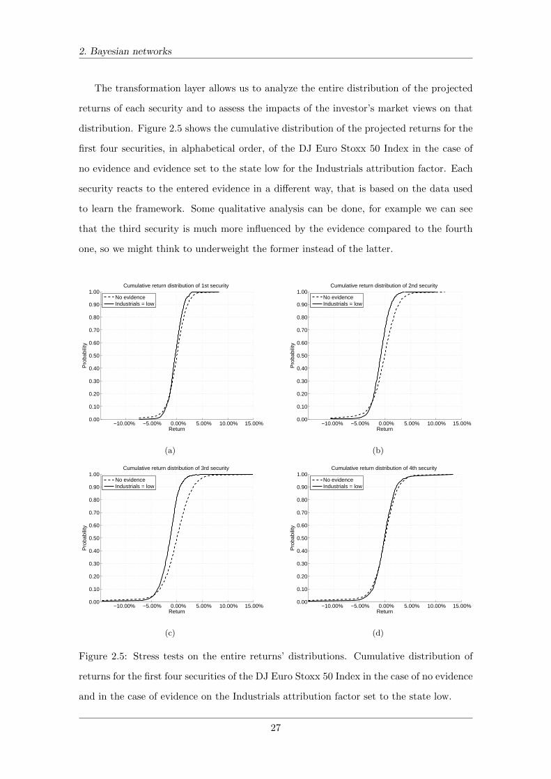
2. Bayesian networks
The transformation layer allows us to analyze the entire distribution of the projected
returns of each security and to assess the impacts of the investor’s market views on that
distribution. Figure 2.5 shows the cumulative distribution of the projected returns for the
first four securities, in alphabetical order, of the DJ Euro Stoxx 50 Index in the case of
no evidence and evidence set to the state low for the Industrials attribution factor. Each
security reacts to the entered evidence in a different way, that is based on the data used
to learn the framework. Some qualitative analysis can be done, for example we can see
that the third security is much more influenced by the evidence compared to the fourth
one, so we might think to underweight the former instead of the latter.
−10.00% −5.00% 0.00% 5.00% 10.00% 15.00%0.00
0.10
0.20
0.30
0.40
0.50
0.60
0.70
0.80
0.90
1.00Cumulative return distribution of 1st security
Return
Pro
babi
lity
No evidenceIndustrials = low
(a)
−10.00% −5.00% 0.00% 5.00% 10.00% 15.00%0.00
0.10
0.20
0.30
0.40
0.50
0.60
0.70
0.80
0.90
1.00Cumulative return distribution of 2nd security
Return
Pro
babi
lity
No evidenceIndustrials = low
(b)
−10.00% −5.00% 0.00% 5.00% 10.00% 15.00%0.00
0.10
0.20
0.30
0.40
0.50
0.60
0.70
0.80
0.90
1.00Cumulative return distribution of 3rd security
Return
Pro
babi
lity
No evidenceIndustrials = low
(c)
−10.00% −5.00% 0.00% 5.00% 10.00% 15.00%0.00
0.10
0.20
0.30
0.40
0.50
0.60
0.70
0.80
0.90
1.00Cumulative return distribution of 4th security
Return
Pro
babi
lity
No evidenceIndustrials = low
(d)
Figure 2.5: Stress tests on the entire returns’ distributions. Cumulative distribution of
returns for the first four securities of the DJ Euro Stoxx 50 Index in the case of no evidence
and in the case of evidence on the Industrials attribution factor set to the state low.
27
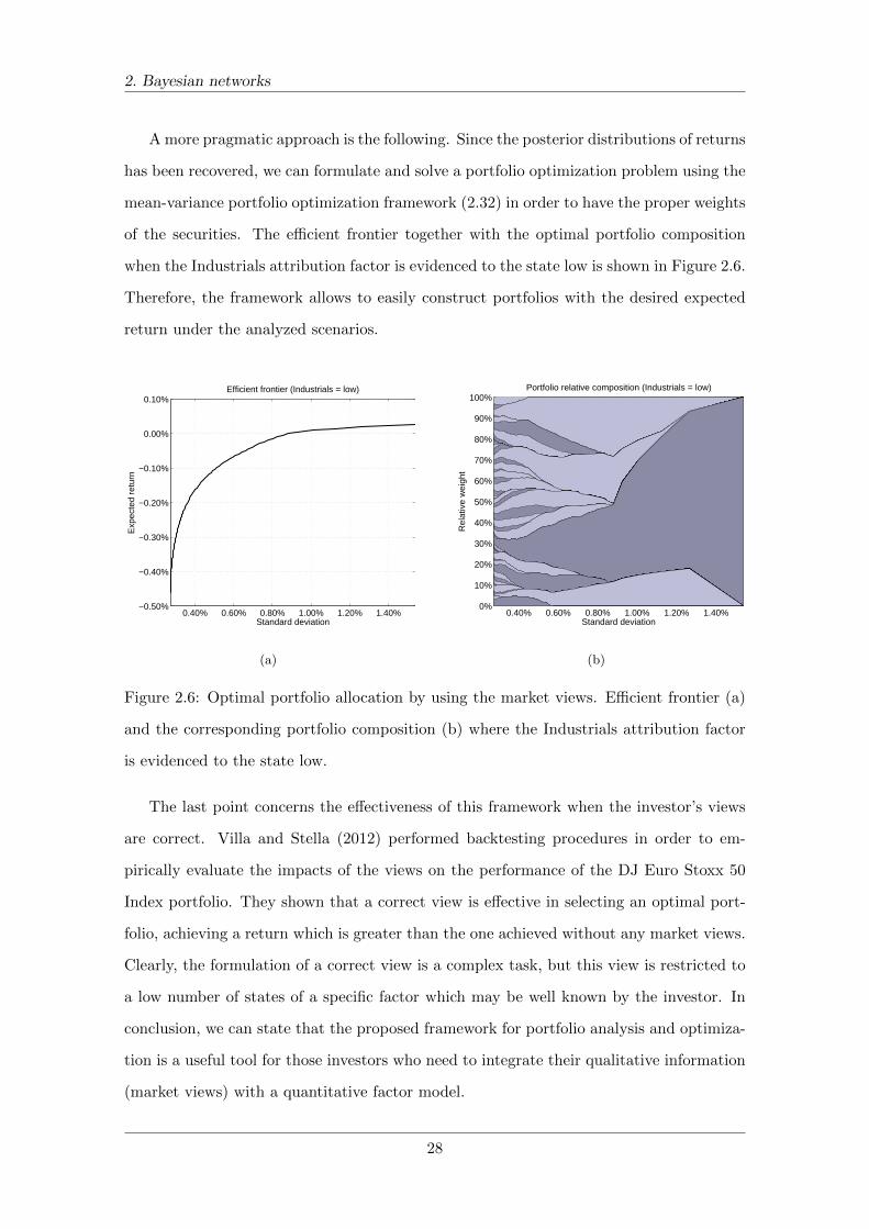
2. Bayesian networks
A more pragmatic approach is the following. Since the posterior distributions of returns
has been recovered, we can formulate and solve a portfolio optimization problem using the
mean-variance portfolio optimization framework (2.32) in order to have the proper weights
of the securities. The efficient frontier together with the optimal portfolio composition
when the Industrials attribution factor is evidenced to the state low is shown in Figure 2.6.
Therefore, the framework allows to easily construct portfolios with the desired expected
return under the analyzed scenarios.
0.40% 0.60% 0.80% 1.00% 1.20% 1.40%−0.50%
−0.40%
−0.30%
−0.20%
−0.10%
0.00%
0.10%Efficient frontier (Industrials = low)
Standard deviation
Exp
ecte
d re
turn
(a)
0.40% 0.60% 0.80% 1.00% 1.20% 1.40% 0%
10%
20%
30%
40%
50%
60%
70%
80%
90%
100%Portfolio relative composition (Industrials = low)
Standard deviation
Rel
ativ
e w
eigh
t
(b)
Figure 2.6: Optimal portfolio allocation by using the market views. Efficient frontier (a)
and the corresponding portfolio composition (b) where the Industrials attribution factor
is evidenced to the state low.
The last point concerns the effectiveness of this framework when the investor’s views
are correct. Villa and Stella (2012) performed backtesting procedures in order to em-
pirically evaluate the impacts of the views on the performance of the DJ Euro Stoxx 50
Index portfolio. They shown that a correct view is effective in selecting an optimal port-
folio, achieving a return which is greater than the one achieved without any market views.
Clearly, the formulation of a correct view is a complex task, but this view is restricted to
a low number of states of a specific factor which may be well known by the investor. In
conclusion, we can state that the proposed framework for portfolio analysis and optimiza-
tion is a useful tool for those investors who need to integrate their qualitative information
(market views) with a quantitative factor model.
28
2. Bayesian networks
2.5 Discussion
In this chapter, we have presented the basic theory about Bayesian networks, a sound
probabilistic graphical tool for modeling and reasoning with uncertain beliefs. We have
discussed the main characteristics of these models, such as their ability to compactly rep-
resent large probability distributions and the availability of inference algorithms that can
effectively answer queries about these distributions. We have explored how it is possible to
learn Bayesian networks from data and how to use them to perform exact and approximate
inference. In the last part of the chapter we have described the interplay between modern
portfolio theory and Bayesian networks and how it is possible to exploit them in a novel
framework for portfolio analysis and optimization. This framework provides an efficient
way to interface models to data and allows efficient evidential reasoning to understand the
behavior of the investment portfolio in different economic scenarios.
29
Chapter 3
Continuous time Bayesian
networks
Continuous time Bayesian networks are probabilistic graphical models which describe
structured stochastic processes that evolve over continuous time. They are based both
on homogeneous Markov processes, as they model the transition dynamics of a system,
and on Bayesian networks, as they provide a graphical representation over a structured
state space. These models are fundamental to the work developed in this thesis. We start
this chapter discussing their representation, we move on to describe how it is possible
to perform learning, we continue by reviewing the inference methods and then we finish
discussing about the related models and applications.
3.1 Representation
The representation power of continuous time Bayesian networks is inherent to the factor-
ization of the system dynamics in local Markov processes that depend on some limited set
of state variables and not on the entire state of the system. We present the necessary
concepts about continuous time Markov processes that are crucial to understanding the
definition and semantics of these models. It should be noted that the first section serves as
background material, if a more detailed description is required, we refer to Norris (1997).
30
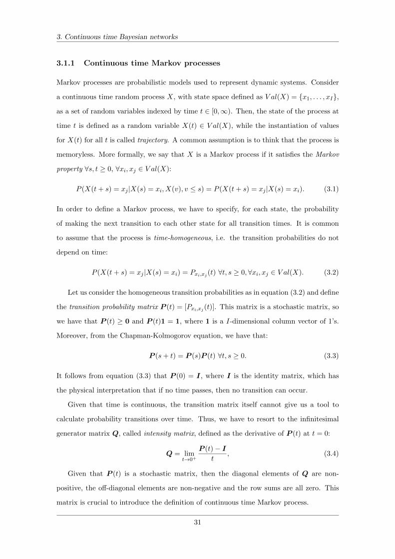
3. Continuous time Bayesian networks
3.1.1 Continuous time Markov processes
Markov processes are probabilistic models used to represent dynamic systems. Consider
a continuous time random process X, with state space defined as V al(X) = {x1, . . . , xI},
as a set of random variables indexed by time t ∈ [0,∞). Then, the state of the process at
time t is defined as a random variable X(t) ∈ V al(X), while the instantiation of values
for X(t) for all t is called trajectory. A common assumption is to think that the process is
memoryless. More formally, we say that X is a Markov process if it satisfies the Markov
property ∀s, t ≥ 0, ∀xi, xj ∈ V al(X):
P (X(t+ s) = xj |X(s) = xi, X(v), v ≤ s) = P (X(t+ s) = xj |X(s) = xi). (3.1)
In order to define a Markov process, we have to specify, for each state, the probability
of making the next transition to each other state for all transition times. It is common
to assume that the process is time-homogeneous, i.e. the transition probabilities do not
depend on time:
P (X(t+ s) = xj |X(s) = xi) = Pxi,xj (t) ∀t, s ≥ 0, ∀xi, xj ∈ V al(X). (3.2)
Let us consider the homogeneous transition probabilities as in equation (3.2) and define
the transition probability matrix P (t) = [Pxi,xj (t)]. This matrix is a stochastic matrix, so
we have that P (t) ≥ 0 and P (t)1 = 1, where 1 is a I-dimensional column vector of 1’s.
Moreover, from the Chapman-Kolmogorov equation, we have that:
P (s+ t) = P (s)P (t) ∀t, s ≥ 0. (3.3)
It follows from equation (3.3) that P (0) = I, where I is the identity matrix, which has
the physical interpretation that if no time passes, then no transition can occur.
Given that time is continuous, the transition matrix itself cannot give us a tool to
calculate probability transitions over time. Thus, we have to resort to the infinitesimal
generator matrix Q, called intensity matrix, defined as the derivative of P (t) at t = 0:
Q = limt→0+
P (t)− It
, (3.4)
Given that P (t) is a stochastic matrix, then the diagonal elements of Q are non-
positive, the off-diagonal elements are non-negative and the row sums are all zero. This
matrix is crucial to introduce the definition of continuous time Markov process.
31
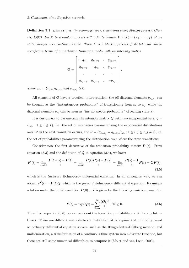
3. Continuous time Bayesian networks
Definition 3.1. (finite states, time-homogeneous, continuous time) Markov process, (Nor-
ris, 1997). Let X be a random process with a finite domain V al(X) = {x1, . . . , xI} whose
state changes over continuous time. Then X is a Markov process iff its behavior can be
specified in terms of a markovian transition model with an intensity matrix
Q =
−qx1 qx1,x2 . qx1,xI
qx2,x1 −qx2 . qx2,xI
. . . .
qxI ,x1 qxI ,x2 . −qxI
,
where qxi =∑
j 6=i qxi,xj and qxi,xj ≥ 0.
All elements of Q have a practical interpretation: the off-diagonal elements qxi,xj can
be thought as the “instantaneous probability” of transitioning from xi to xj , while the
diagonal elements qxi can be seen as “instantaneous probability” of leaving state xi.
It is customary to parametrize the intensity matrix Q with two independent sets: q =
{qxi : 1 ≤ i ≤ I}, i.e. the set of intensities parameterizing the exponential distributions
over when the next transition occurs, and θ = {θxi,xj = qxi,xj/qxi : 1 ≤ i, j ≤ I, j 6= i}, i.e.
the set of probabilities parameterizing the distribution over where the state transitions.
Consider now the first derivative of the transition probability matrix P ′(t). From
equation (3.3) and the definition of Q in equation (3.4), we have:
P ′(t) = lims→0+
P (t+ s)− P (t)
s= lim
s→0+
P (t)P (s)− P (s)
s= lim
s→0+
P (s)− Is
P (t) = QP (t),
(3.5)
which is the backward Kolmogorov differential equation. In an analogous way, we can
obtain P ′(t) = P (t)Q, which is the forward Kolmogorov differential equation. Its unique
solution under the initial condition P (0) = I is given by the following matrix exponential:
P (t) = exp(Qt) =∞∑k=0
(Qt)k
k!, ∀t ≥ 0. (3.6)
Thus, from equation (3.6), we can work out the transition probability matrix for any future
time t. There are different methods to compute the matrix exponential, primarily based
on ordinary differential equation solvers, such as the Runge-Kutta-Fehlberg method, and
uniformization, a transformation of a continuous time system into a discrete time one, but
there are still some numerical difficulties to compute it (Moler and van Loan, 2003).
32
3. Continuous time Bayesian networks
3.1.2 The CTBN model
Continuous time Bayesian networks provide a factored representation of Markov processes
over systems whose state is defined as an assignment to some (possibly large) set of vari-
ables. Using the same idea of Bayesian networks, the dynamics of the entire Markov
process are decomposed in local dynamics according to a graph structure whose nodes are
variables, and the evolution of each variable X depends on the state of its parents Pa(X)
in the graph. These local dynamics are modeled using a special type of Markov process
defined as follows.
Definition 3.2. Conditional Markov process, (Nodelman et al., 2002). Let X be a variable
whose domain is V al(X) = {x1, . . . , xI}. Assume that X evolves as a Markov process X(t)
whose dynamics are conditioned on a set Pa(X) of variables, each of which can also evolve
over time. Then, we have a conditional intensity matrix (CIM) QX|Pa(X) defined as set
of intensity matrices, one for each instantiation pau ∈ Pa(X):
QX|pau =
−qx1|pau qx1,x2|pau . qx1,xI |pau
qx2,x1|pau −qx2|pau . qx2,xI |pau
. . . .
qxI ,x1|pau qxI ,x2|pau . −qxI |pau
.
Clearly, if Pa(X) = ∅, then the CIM is the intensity matrix of a standard Markov
process. Conditional intensity matrices are the building blocks of the dynamic component
of a continuous time Bayesian network, that is defined as follows:
Definition 3.3. Continuous time Bayesian network (CTBN), (Nodelman et al., 2002).
Let X be a set of random variables X1, . . . , XN . Each X has a finite domain of values
V al(X) = {x1, . . . , xI}. A continuous time Bayesian network N = (B,M) over X con-
sists of two components: the first is an initial distribution P 0X , specified as a Bayesian
network B over X, the second is a continuous time transition model M specified as:
• a directed (possibly cyclic) graph G whose nodes are X1, . . . , XN ;
• a conditional intensity matrix, QX|Pa(X), for each variable X ∈X.
33

3. Continuous time Bayesian networks
3.1.3 Semantics
It is possible to define the semantics of the CTBN model as a single Markov process over
the joint state space using a special type of operator called amalgamation (Nodelman
et al., 2002). This operator takes two CIMs and produces as output a single bigger CIM.
Intuitively, given two sets of variables Y = Y 1 ∪ Y 2 ⊆ X and Z = Z1 ∪ Z2 ⊆ X \ Y ,
and two CIMs QY 1|Z1and QY 2|Z2
, the amalgamated CIM QY |Z = QY 1|Z1× QY 2|Z2
contains the intensities for the variables in Y conditioned on those in Z.
Therefore, a CTBN N is a factored representation of an homogeneous Markov process
described by the joint intensity matrix:
QN =∏X∈X
QX|Pa(X), (3.7)
where here the symbol∏
refers to the amalgamation operator. We note that QN is a
square matrix over the entire joint state space with cardinality equals to the product the
cardinality of each variable X ∈X.
The CTBN model can be also seen as a generative model over sequences of events,
where an event is a pair (t,x[xn]) which denotes a transition of the variable Xn to the
value xn ∈ V al(Xn) at time t. The generative procedure takes the initial distribution, the
description of each variable and an end time, and it randomly samples a trajectory for the
system from the initial time to end time (Nodelman et al., 2002).
It is noteworthy to mention two important aspects of this model compared to the stan-
dard Bayesian networks framework. Firstly, like BNs, the graph of CTBNs provides both
a skeleton for representing the joint distribution and a description of the independence
properties of this distribution. Unlike BNs, the graph of a CTBN specifies a notion of
independence over entire trajectories and it can contain cycles because it refers to the
dynamic component of the system. In fact, an arc X → Y implies that the temporal
dynamics of Y depends on the value of X, while a loop X ↔ Y implies that the temporal
dynamics of X simultaneously depend on the value of Y and vice versa. Secondly, a fun-
damental assumption in CTBNs in that, as time is continuous, variables cannot transition
at the same instant. Thus, all intensities corresponding to two simultaneous changes are
zero (Nodelman, 2007). This assumption will be crucial for the algorithms designed in the
next chapters.
34
3. Continuous time Bayesian networks
3.2 Learning
Continuous time Bayesian networks can be learned directly from data, and then they can
be used to perform inference or knowledge discovery. As in the context of the BNs frame-
work, the likelihood of the data is decomposed into local likelihoods and it is summarized
in terms of sufficient statistics aggregated over the data. We discuss the basic notions
of parameter and structural learning of the dynamic component of a CTBN. Parameter
learning is concerned with the estimation of the elements of the CIMs when the graph
is known, while structural learning is concerned with the selection of the graph and the
estimation of the CIMs. Parametric and structural learning can be developed for complete
or missing data arising from partial observability of the trajectory. We cover the first case,
while we refer to Nodelman et al. (2003) for the second case.
3.2.1 Parameter learning
In the parameter learning case, the graph G of the CTBN is given and the goal is to learn
each entry of each intensity matrix QX|pau that governs the dynamics of X. Given that
a CTBN N describes a Markov process over the joint state space, we can parametrize it
using q and θ, while we use qX|pau and θX|pau to parametrize each intensity matrix.
Given a data set D = {σ1, . . . ,σM} of M fully observed trajectories, where each σ is a
complete set of state transitions and the times at which they occurred, then the likelihood
function decomposes by variable and parameter as follows:
LN (q,θ : D) =∏X∈X
LX(qX|Pa(X) : D) LX(θX|Pa(X) : D). (3.8)
The formulation (3.8) allows us to maximize each local likelihood LX independently and
then to combine them to get the MLE parameters. The likelihood of the data set can be
expressed in terms of the following sufficient statistics (Nodelman et al., 2003):
• T [xi|pau]: the amount of time spent in the state X = xi while Pa(X) = pau;
• M [xi, xj |pau]: the number of transitions from X = xi to X = xj while Pa(X) =
pau. From this statistic, we have that M [xi|pau] =∑
xj 6=xiM [xi, xj |pau]: the total
number of transitions leaving the state X = xi while Pa(X) = pau.
35
3. Continuous time Bayesian networks
The component LX(θX|Pa(X) : D) of equation (3.8) gives us the probability of the
sequence of state transitions that depend only on the value of the parents at the instant
of the transition. Thus, as done in the BNs context, we can decompose the parameter
θX|Pa(X) of each variable X ∈X by a set of parameters θxi,xj |pau for each xi, xj ∈ V al(X)
with xj 6= xi and instantiation of its parents pau ∈ Pa(X). Thus, the local likelihood of
the parameter θ can be written as follows:
LX(θX|Pa(X) : D) =∏pau
∏xi
∏xj 6=xi
θM [xi,xj |pau]
xi,xj |pau . (3.9)
The component LX(qX|Pa(X) : D) of equation (3.8) gives us the probability that X
stays in a state xi under a specific parent configuration pau ∈ Pa(X). The duration in
the state xi can be determined by a transition of X or a transition of one of its parents.
Thus, the local likelihood of the parameter q can be written as follows:
LX(qX|Pa(X) : D) =∏pau
∏xi
qM [xi|pau]xi|pau exp
(−qxi|pauT [xi|pau]
). (3.10)
The maximization of the likelihood in equation (3.8) can be performed using the fol-
lowing MLE parameters as a function of the sufficient statistics (Nodelman et al., 2003):
qxi|pau =M [xi|pau]
T [xi|pau], θxi,xj |pau =
M [xi, xj |pau]
M [xi|pau]. (3.11)
An alternative to MLE is the Bayesian parameter estimation. This estimation can be
performed in a similar way to the BNs case, where P (qG ,θG |D) ∝ P (D|qG ,θG)P (qG ,θG).
For the prior over parameters P (qG ,θG), we assume independence between the sets of
parameters characterizing the exponential distributions and the set of parameters charac-
terizing the multinomial distributions:
P (qG ,θG) = P (qG |G)P (θG |G). (3.12)
We assume global parameter independence (2.10), so we have that:
P (qG ,θG) =∏X∈X
P (qX|Pa(X)|G)P (θX|Pa(X)|G), (3.13)
and local parameter independence (2.11), thus we have that:
P (qG ,θG) =∏X∈X
∏pau
∏xi
P (qxi|pau |G)P (θxi|pau |G). (3.14)
36
3. Continuous time Bayesian networks
For a Markov process, it is customary to choose a Dirichlet distribution as prior for
the parameters corresponding to the multinomial distribution, while we choose a gamma
distribution as prior for the parameter corresponding to the exponential distribution:
P (qxi) ∼Gamma (αxi , τxi) , (3.15)
P (θxi) ∼Dir (αxi,x1 , . . . , αxi,xI ) . (3.16)
After conditioning on the data set D, we have:
P (qxi |D) ∼Gamma (αxi +M [xi], τxi + T [xi]) , (3.17)
P (θxi |D) ∼Dir (αxi,x1 +M [xi, x1], . . . , αxi,xI +M [xi, xI ]) . (3.18)
As in the BNs case, these posteriors can be used to predict the next event, averaging out
the event probability over the possible values of the parameters, that is equivalent to use
the following parameters:
qxi|pau =αxi|pau +M [xi|pau]
τxi|pau + T [xi|pau], θxi,xj |pau =
αxi,xj |pau +M [xi, xj |pau]
αxi|pau +M [xi|pau], (3.19)
where α represents the pseudocount of the number of transitions from one state to another
and τ represents the imaginary amount of time spent in each state (Nodelman, 2007).
3.2.2 Structural learning
The problem of learning the structure of a CTBN is simpler then the general BN case
because we do not have to satisfy any acyclic constraint. In this case, we resort to a
score-based approach defining a Bayesian score and then searching (without constraints)
a structure that has the highest score. The Bayesian score is the same as the BNs case
(2.16) that we report here for convenience:
BS(G : D) = lnP (G) + lnP (D|G). (3.20)
As the prior over structure P (G) does not grow with the size of data, the significant term
of the Bayesian score is the marginal likelihood of the data, given the structure P (D|G).
This term is computed by marginalizing out the unknown parameters as follows:
P (D|G) =
∫qG ,θG
P (D|qG ,θG ,G)P (qG ,θG |G)dqGdθG . (3.21)
37
3. Continuous time Bayesian networks
In the case of no missing values, the probability of the data given a CTBN model
P (D|qG ,θG ,G) can be decomposed as a product of likelihoods as shown in equation (3.8):
P (D|qG ,θG ,G) =∏X∈X
LX(qX|Pa(X) : D) LX(θX|Pa(X) : D). (3.22)
Using the global parameter independence assumption (2.10) and the decomposition
(3.22), the marginal likelihood P (D|G) can be written as follows:
P (D|G) =∏X∈X
∫qG
LX(qX|Pa(X) : D)P (qX|Pa(X))dqG (3.23)
×∏X∈X
∫θG
LX(θX|Pa(X) : D)P (θX|Pa(X))dθG (3.24)
=∏X∈X
MLX(qX|Pa(X) : D)×MLX(θX|Pa(X) : D). (3.25)
It is possible to extend the BDe metric of BNs and to compute the marginal likelihood
P (D|G) in closed form, given the sufficient statistics over the data. Therefore, the closed
form solution of the marginal likelihood of q reported in equation (3.23) is:
∏pau
∏xi
Γ(αxi|pau +M [xi|pau] + 1
) (τxi|pau
)(αxi|pau+1)
Γ(αxi|pau + 1
) (τxi|pau + T [xi|pau]
)(αxi|pau+M [xi|pau]+1), (3.26)
and the marginal likelihood of θ reported in equation (3.24) is:
∏pau
∏xi=xj
Γ(αxi|pau
)Γ(αxi|pau +M [xi|pau]
) × ∏xi 6=xj
Γ(αxi,xj |pau +M [xi, xj |pau]
)Γ(αxi,xj |pau
) . (3.27)
Using the closed form solutions (3.26) and (3.27), under the assumption of structure
modularity (2.17), the Bayesian score can be decomposed by variable as follows:
BS(G : D) =∑X∈X
lnP (Pa(X) = PaG(X))
+ lnMLX(qX|Pa(X) : D) + lnMLX(θX|Pa(X) : D). (3.28)
Since there are no acyclic constraints, it is possible to optimize the parent set for each
variable independently and then combining the results. Thus, the search space over the
graph structures can be done in polynomial time, given a maximum number of possible
parents per variable. The search can be easily performed enumerating each possible parent
set or using a greedy hill-climbing search with operators that add and delete edges in the
graph.
38
3. Continuous time Bayesian networks
3.3 Inference
Since a continuous time Bayesian network is a compact representation of a joint intensity
matrix for a Markov process, it can be used to answer any query that we can answer
using a state-space model, such as filtering, prediction and smoothing (Murphy, 2002).
In the CTBN context, there are two types of possible evidence: point evidence, it is an
observation of the value xi of a variable X at a particular instant in time, i.e. X(t) = xi,
and continuous evidence, it is an observation of the value of a variable throughout an
entire interval which we take to be a half-closed interval [t1; t2), i.e. X[t1 : t2) = xi[t1 : t2).
Using a CTBN model we can ask about the marginal distribution of some variables at
a particular time, e.g. the distribution of X1(t) = x1 and X2(t) = x2 at t = 5, or queries
about the timing of a transition, e.g. the distribution over the time that X1 transitions
from x1 to x2 in the time interval [0; 5). Other common types of queries are related to
the expected sufficient statistics, such as the expected amount of time that a variable X1
spends in a state x1, i.e. E[T [x1]], and the expected number of times that a variable X1
transitions from state x1 to state x2, i.e. E[M [x1, x2]].
After a brief discussion about the difficulties associated with exact inference (Nodelman
et al., 2002), we show how it is possible to perform approximate inference using sampling-
based approaches similar to the BNs case (Fan and Shelton, 2008).
3.3.1 Exact inference
Given a series of observations, we can calculate the joint distribution using equation (3.7)
at the time of the first observation, conditioned on that observation, and use this new
distribution as the initial one from which to compute the joint distribution at the time of
the next observation. The limit of this inference procedure is that the generation of the
full joint intensity matrix is exponential in the number of variables.
Unfortunately, the graph structure of the CTBN cannot help us to decompose the
problem. For example, consider the simplest case of connection depicted in Figure 2.1
(a), X → Z → Y , where Z is instantiated. In the BN model, if the state of Z is
known, then X and Y become independent. Conversely, in the CTBN model, even if the
transition intensity of Y depends only on the value of Z at any point in time, as soon as
39
3. Continuous time Bayesian networks
we consider temporal evolution, their states become correlated. This phenomenon, called
entanglement, is an effect present also in other temporal models which causes independent
random variables (considered point in time) to have a dependency (over time) due to
frequent updates (Nodelman et al., 2002). Therefore, the only possible conclusion we can
make is that X is independent of Y given the full trajectory of Z. Unfortunately, also the
reconstruction of the full trajectory cannot be performed compactly. Thus, we have to
resort to approximate methods to perform inference in a general CTBN model.
3.3.2 Approximate inference
Several approximate algorithms have been proposed in the literature. Nodelman et al.
(2005a) introduced the expectation propagation algorithm which allows both point and
continuous evidence. Friedman and Kupferman (2006) demonstrated that a separation of
time scales between variables can lead to a simpler inference problem. Saria et al. (2007)
presented an improved approximate inference method based on expectation propagation.
Alternatives are offered by mean field variational approximation (Cohn et al., 2009) and
continuous time belief propagation (El-Hay et al., 2010) algorithms. Sampling-based algo-
rithms, such as importance sampling (Fan and Shelton, 2008) and Gibbs sampling (El-Hay
et al., 2008; Rao and Teh, 2011) have been introduced. We describe the basic notions of
the importance sampling algorithm that has the advantage of being an anytime algorithm,
i.e. it is possible to stop it at any time during the computation to obtain an answer and,
in the limit, it converges to the true answer.
As in the case of BNs, we can use forward sampling to answer any query that is not
conditioned on evidence. This procedure is based on randomly sampling many particles
and looking at the fraction that matches the query. Note that, in the context of CTBNs, a
particle is a sampled trajectory. Formally, given a set D = {σ1, . . . ,σM} of M trajectories,
we can estimate the expectation of any function f by computing:
ED[f ] =1
M
M∑m=1
f(σm). (3.29)
Thus, if we would like to estimate P (X(5) = x1), then we can use f = 1{X(5)=x1}. The
function f can also count the total number of times that X transitions from x1 to x2 while
Pa(X) = pa3, allowing us to estimate the expected sufficient statistic M [x1, x2|pa3].
40

3. Continuous time Bayesian networks
If we would like to answer any query that is conditioned on evidence, then we have
to resort to other techniques, such as (normalized) importance sampling. Given a set of
samples D′ = {σ′1, . . . ,σ′M} of M trajectories from a proposal distribution P ′, the estimate
of the conditional expectation of a function f given an evidence e is:
ED[f |e] =1
W
M∑m=1
f(σ′m)w(σ′m), (3.30)
where W is the sum of the weights, i.e. the normalization factor.
If the query involves an evidence over some subset of variables Y ⊂ X for the total
length of the trajectory, then we force the behavior of these variables. Specifically, the
proposal distribution is obtained by forward sampling the behavior of variables X ∈X \Y
and inserting the known transitions at known times for variables in Y . As in the BNs
case, given that the weight is the ratio of the likelihood contributions of all variables X
against X \ Y , then the weight can be computed as:
w(σ′) =PN (σ′)
P ′(σ′)=
∏X∈X
∏Jj=0 LX(x[τj : τj+1))∏
X∈X\Y∏Jj=0 LX(x[τj : τj+1))
=∏X∈Y
J∏j=0
LX(x[τj : τj+1)), (3.31)
where τ0 = 0, . . . , τJ+1 = T are the transition times in the interval [0;T ) for a trajectory.
If the query involves evidence where variables are both observed and unobserved, then
we force the trajectory to be consistent with it by looking ahead for each variable we
sample. If the current state does not agree with the upcoming evidence, then we sample
the next transition time ∆t from a truncated exponential distribution. Let tbe be the time
where the evidence begins, σ′be be the set for all variables X ∈ X of intervals x[τj : τj+1)
where the behavior of X is set by the evidence and σ′co be the complement of σ′be containing
the set of intervals of unobserved behavior for all variables. We have that:
w(σ′) =PN (σ′)
P ′(σ′)=
∏x[τj :τj+1)∈σ′co
LX(x[τj : τj+1))
L′X(x[τj : τj+1))×
∏x[τj :τj+1)∈σ′be
LX(x[τj : τj+1)). (3.32)
We can have four cases. For any variable X whose value is given by the evidence during
the interval [t; t+∆t), the contribution to the trajectory weight is the likelihood as before.
For any variable X whose ∆t was sampled from an exponential distribution, the ratio in
equation (3.32) is 1. For any variable X whose ∆t was sampled from a truncated exponen-
tial distribution, if it is involved in the next transition, then the ratio is 1−exp(−q(tbe−t)),
otherwise the ratio is 1−exp(−q(tbe−t))1−exp(−q(tbe−t−∆t)) that is almost 1 when ∆t is small.
41
3. Continuous time Bayesian networks
3.4 Related models and applications
Different models have been developed to handle temporal reasoning using the general
BNs framework, among them the well known dynamic Bayesian networks. Continuous
time Bayesian networks made a significant contribution in this field proving a factored
representation of continuous time Markov processes and making available inference and
learning algorithms. Some assumption underpinning the CTBN model have been relaxed
in order to cover a wider range of systems. The increase of the number of applications
to real life problems reveals the effectiveness of the CTBN model. We provide a brief
survey about dynamic Bayesian networks, temporal Bayesian networks, and the latest
developments and applications of continuous time Bayesian networks.
3.4.1 Dynamic Bayesian networks
Dynamic Bayesian networks (Dean and Kanazawa, 1989) are an extension of BNs to model
probability distributions over a collection of random variables X0,X1,X2, . . . . Under the
Markov assumption and the time-homogeneity of the transition dynamics, it is possible
to compactly represent the probability distribution over infinite trajectories by means of
an initial state distribution and a transition model that specifies a conditional probability
distribution between current time variables X and next time step variables X ′.
Definition 3.4. Dynamic Bayesian network (DBN), (Murphy, 2002). A dynamic Bayesian
network over a set of random variables {X1, . . . , XN , X′1, . . . , X
′N} is a pair B2 = (B0,B2T ),
where B0 is a Bayesian network which defines a prior distribution P (X), and B2T is a
two-slice temporal Bayes network which defines
P (X ′|X) =∏X′∈X
P (X ′|Pa(X ′)) (3.33)
by means of a directed acyclic graph in which edges can connect nodes between two time
slices (inter-time) or nodes in the same time slice (intra-time).
Given a distribution over the initial states, it is possible to unroll the network over
sequences of a given length in order to create a new BN that induces a distribution over
trajectories of that length. DBNs can be learned directly from data and they can be
used to perform filtering, prediction and smoothing tasks. Unfortunately, if there are long
observation sequences, inference becomes impractical in complex DBNs (Murphy, 2002).
42

3. Continuous time Bayesian networks
Even if both DBNs and CTBNs allow us to model dynamic systems, they are naturally
different. A DBN can be seen as a model of a sequence of observations as it learns a series of
snapshots of the system; indeed the learned model can be very sensitive to the granularity
of the time step chosen. Conversely, a CTBN can be interpreted as a model of the system
as it learns a series of state transitions produced by the system itself. In conclusion,
DBNs can be successfully applied in domains where the data is intrinsically time-sliced
and where queries about events occurring between time points are not relevant. For all
other domains, it is convenient to use CTBNs as they do not require to choose a fixed time
step and the number of parameters to estimate is significantly lower compared to DBNs.
3.4.2 Bayesian temporal models
Three main streams of research have attempted to model temporal reasoning in the
Bayesian network framework. The first one consists of instant-based formalisms, in which
time is discretized in fixed-size intervals and an instance of each random variable is created
for each point in time. The models belonging to this group are closely related to DBNs.
The second group are interval-based formalisms, such as temporal Bayesian networks
(Tawfik and Neufeld, 1994), temporal nodes Bayesian networks (Arroyo-Figueroa and Su-
car, 1999) and probabilistic temporal networks (Santos and Young, 1999). In these models,
time is usually discretized into a finite number of intervals that can be of different size and
duration for each node, allowing to handle multiple granularity. Each model is based on
its own graphical semantics. For example, in temporal nodes Bayesian networks, a node
represents an event or a state change of a variable, while an arc between two nodes corre-
sponds to a causal-temporal relation. Conversely, in the probabilistic temporal networks,
nodes are temporal aggregates that represent the process changing over time and arcs are
the causal-temporal relationships between aggregates.
The last group are formalisms based on a representation of time as continuous variables,
such as networks of dates (Berzuini, 1989) and continuous time nets (Kanazawa, 1992).
In these models, the time to occurrence of significant events is generally modeled using
continuous time survival analysis, but the temporal distributions generated are not used
for modeling state durations of local variables. Therefore, they are more related to the
classical event history analysis (Aalen et al., 2008) compared to Bayesian networks.
43
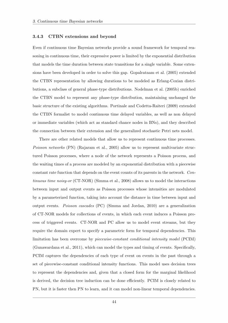
3. Continuous time Bayesian networks
3.4.3 CTBN extensions and beyond
Even if continuous time Bayesian networks provide a sound framework for temporal rea-
soning in continuous time, their expressive power is limited by the exponential distribution
that models the time duration between state transitions for a single variable. Some exten-
sions have been developed in order to solve this gap. Gopalratnam et al. (2005) extended
the CTBN representation by allowing durations to be modeled as Erlang-Coxian distri-
butions, a subclass of general phase-type distributions. Nodelman et al. (2005b) enriched
the CTBN model to represent any phase-type distribution, maintaining unchanged the
basic structure of the existing algorithms. Portinale and Codetta-Raiteri (2009) extended
the CTBN formalist to model continuous time delayed variables, as well as non delayed
or immediate variables (which act as standard chance nodes in BNs), and they described
the connection between their extension and the generalized stochastic Petri nets model.
There are other related models that allow us to represent continuous time processes.
Poisson networks (PN) (Rajaram et al., 2005) allow us to represent multivariate struc-
tured Poisson processes, where a node of the network represents a Poisson process, and
the waiting times of a process are modeled by an exponential distribution with a piecewise
constant rate function that depends on the event counts of its parents in the network. Con-
tinuous time noisy-or (CT-NOR) (Simma et al., 2008) allows us to model the interactions
between input and output events as Poisson processes whose intensities are modulated
by a parameterized function, taking into account the distance in time between input and
output events. Poisson cascades (PC) (Simma and Jordan, 2010) are a generalization
of CT-NOR models for collections of events, in which each event induces a Poisson pro-
cess of triggered events. CT-NOR and PC allow us to model event streams, but they
require the domain expert to specify a parametric form for temporal dependencies. This
limitation has been overcome by piecewise-constant conditional intensity model (PCIM)
(Gunawardana et al., 2011), which can model the types and timing of events. Specifically,
PCIM captures the dependencies of each type of event on events in the past through a
set of piecewise-constant conditional intensity functions. This model uses decision trees
to represent the dependencies and, given that a closed form for the marginal likelihood
is derived, the decision tree induction can be done efficiently. PCIM is closely related to
PN, but it is faster then PN to learn, and it can model non-linear temporal dependencies.
44
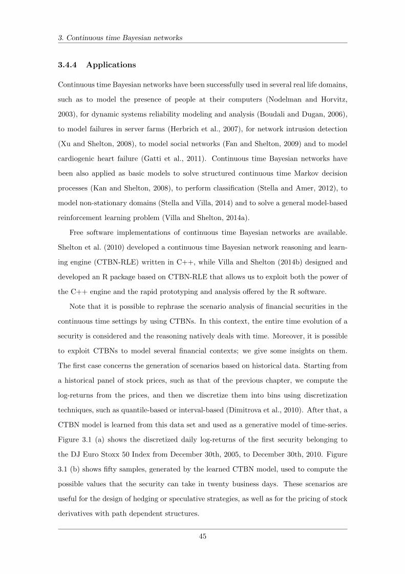
3. Continuous time Bayesian networks
3.4.4 Applications
Continuous time Bayesian networks have been successfully used in several real life domains,
such as to model the presence of people at their computers (Nodelman and Horvitz,
2003), for dynamic systems reliability modeling and analysis (Boudali and Dugan, 2006),
to model failures in server farms (Herbrich et al., 2007), for network intrusion detection
(Xu and Shelton, 2008), to model social networks (Fan and Shelton, 2009) and to model
cardiogenic heart failure (Gatti et al., 2011). Continuous time Bayesian networks have
been also applied as basic models to solve structured continuous time Markov decision
processes (Kan and Shelton, 2008), to perform classification (Stella and Amer, 2012), to
model non-stationary domains (Stella and Villa, 2014) and to solve a general model-based
reinforcement learning problem (Villa and Shelton, 2014a).
Free software implementations of continuous time Bayesian networks are available.
Shelton et al. (2010) developed a continuous time Bayesian network reasoning and learn-
ing engine (CTBN-RLE) written in C++, while Villa and Shelton (2014b) designed and
developed an R package based on CTBN-RLE that allows us to exploit both the power of
the C++ engine and the rapid prototyping and analysis offered by the R software.
Note that it is possible to rephrase the scenario analysis of financial securities in the
continuous time settings by using CTBNs. In this context, the entire time evolution of a
security is considered and the reasoning natively deals with time. Moreover, it is possible
to exploit CTBNs to model several financial contexts; we give some insights on them.
The first case concerns the generation of scenarios based on historical data. Starting from
a historical panel of stock prices, such as that of the previous chapter, we compute the
log-returns from the prices, and then we discretize them into bins using discretization
techniques, such as quantile-based or interval-based (Dimitrova et al., 2010). After that, a
CTBN model is learned from this data set and used as a generative model of time-series.
Figure 3.1 (a) shows the discretized daily log-returns of the first security belonging to
the DJ Euro Stoxx 50 Index from December 30th, 2005, to December 30th, 2010. Figure
3.1 (b) shows fifty samples, generated by the learned CTBN model, used to compute the
possible values that the security can take in twenty business days. These scenarios are
useful for the design of hedging or speculative strategies, as well as for the pricing of stock
derivatives with path dependent structures.
45
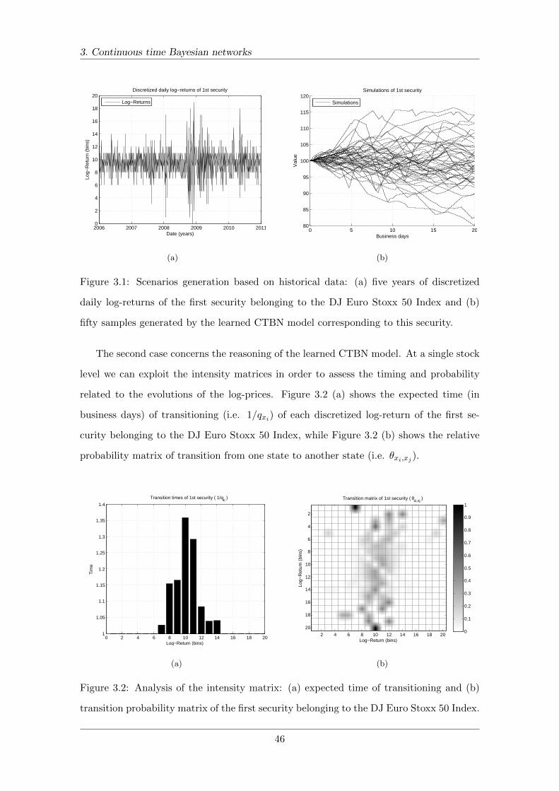
3. Continuous time Bayesian networks
2006 2007 2008 2009 2010 20110
2
4
6
8
10
12
14
16
18
20
Date (years)
Log−
Ret
urn
(bin
s)Discretized daily log−returns of 1st security
Log−Returns
(a)
0 5 10 15 2080
85
90
95
100
105
110
115
120
Business days
Val
ue
Simulations of 1st security
Simulations
(b)
Figure 3.1: Scenarios generation based on historical data: (a) five years of discretized
daily log-returns of the first security belonging to the DJ Euro Stoxx 50 Index and (b)
fifty samples generated by the learned CTBN model corresponding to this security.
The second case concerns the reasoning of the learned CTBN model. At a single stock
level we can exploit the intensity matrices in order to assess the timing and probability
related to the evolutions of the log-prices. Figure 3.2 (a) shows the expected time (in
business days) of transitioning (i.e. 1/qxi) of each discretized log-return of the first se-
curity belonging to the DJ Euro Stoxx 50 Index, while Figure 3.2 (b) shows the relative
probability matrix of transition from one state to another state (i.e. θxi,xj ).
0 2 4 6 8 10 12 14 16 18 201
1.05
1.1
1.15
1.2
1.25
1.3
1.35
1.4
Transition times of 1st security ( 1/qxi )
Log−Return (bins)
Tim
e
(a)
Log−Return (bins)
Log−
Ret
urn
(bin
s)
Transition matrix of 1st security ( θxi,xj )
2 4 6 8 10 12 14 16 18 20
2
4
6
8
10
12
14
16
18
200
0.1
0.2
0.3
0.4
0.5
0.6
0.7
0.8
0.9
1
(b)
Figure 3.2: Analysis of the intensity matrix: (a) expected time of transitioning and (b)
transition probability matrix of the first security belonging to the DJ Euro Stoxx 50 Index.
46
3. Continuous time Bayesian networks
We can also perform analysis that involves multiple stocks. For example, we can
discretize the previous data set into binary values corresponding to positive (denoted as
1) and negative (denoted as 0) returns, we can select the stocks belonging to one sector,
such as the telecommunication sector, and its relative index. A CTBN model is learned
from this data set by imposing a loop structure from a security to its index and vice versa.
In fact, we assume that a security does not influence all other securities in the same sector,
but only the index, which in turn influences the other stocks that compose it. Figure 3.3
(a) shows a possible scenario of the telecommunication stocks belonging to the DJ Euro
Stoxx 50 Index. Note that a scenario consists of the full trajectories of the securities
and not only a single value as in the static case. Figure 3.3 (b) shows the probability of
a positive value of the telecommunication index, given the previous scenario where the
index value in unknown. Therefore, it is possible to infer the temporal evolution of the
index value when the index is not observed, i.e. we can perform filtering. This is useful
in the scenario analysis context where some financial variables are not observed and we
would like to asses their values.
0
1
2Telecommunication stocks scenario
Tel
DE
0
1
2
Tel
FR
0
1
2
Tel
IT
0 2 4 6 8 10 12 14 16 18 20−1
0
1
2
Business days
Tel
ES
(a)
0 2 4 6 8 10 12 14 16 18 20
0.4
0.5
0.6
0.7
0.8
0.9
1
Business days
Pro
babi
lity
Telecommunication Index (probability of a positive value)
(b)
Figure 3.3: Scenario analysis. (a) a possible scenario of the telecommunication stocks
belonging to the DJ Euro Stoxx 50 Index and (b) probability of a positive value of the
telecommunication index given the scenario (a) where the index value in unknown.
47

3. Continuous time Bayesian networks
3.5 Discussion
We have presented the basic theory about continuous time Bayesian networks, a robust
modeling language for structured stochastic processes that evolve over continuous time.
They allow us to model processes without needing to select a temporal granularity and
they make possible the use of cyclic graphs to model mutual influence among random
variables. We have explored how it is possible to learn these models directly from data
and to use them to perform inference. In this case, structural learning with complete data
is simpler then the general Bayesian network case, as there are no acyclic constraints.
Thus, the search space over the graph structures can be done in polynomial time, given a
maximum number of possible parents per variable. On the other hand, exact inference is
limited to the generation of the full joint intensity matrix that is exponential in the number
of variables. Thus, we have to resort to approximate methods to perform inference such as
sampling-based algorithms. Finally, we have discussed the limitations of continuous time
Bayesian networks, their extensions and their applications in several contexts.
48
Chapter 4
Continuous time Bayesian network
classifiers
Continuous time Bayesian networks have been extended to solve the problem of classifi-
cation on multivariate trajectories evolving in continuous time. We start this chapter by
introducing the basic concepts of the classification task and how both Bayesian networks
and dynamic Bayesian networks can be seen as classifiers. We continue reviewing temporal
classification using continuous time Bayesian network classifiers, we move on to describe
an efficient scalable parallel algorithm to learning this latter model from Big Data and
then we finish presenting an application of continuous time Bayesian network classifiers
to the foreign exchange rate prediction problem in high frequency domain.
4.1 Basics
Supervised learning is a basic task of machine learning and it consists of learning an
input-output mapping from a training data set of M observations D = {d1, . . . ,dM}.
Each observation is an input-output pair d = (x, y), where the input x is an instantiation
of X = {X1, . . . , XN} variables called attributes (or features), while the output y is an
instantiation of the class variable Y that can be categorical or scalar. In the first case,
the problem is known as classification, while in the second case the problem is known as
regression. We present the necessary concepts and Bayesian models of classification, while
we refer to Mitchell (1997); Duda et al. (2000); Murphy (2012) for review.
49
4. Continuous time Bayesian network classifiers
4.1.1 Classification
Classification is widely used in machine learning to solve many interesting real life prob-
lems, such as document classification, image classification and handwriting recognition,
and object detection and recognition (Murphy, 2012). We focus on the classification task
of input vectors x of discrete-valued features and output y ∈ V al(Y ) = {y1, . . . , yC},
where C is the number of classes, such that the ultimate goal is to construct a classifier.
A classifier can be defined as function f that assigns a class label to instances described
by a set of attributes, yc = f(x). The learning task concerns the estimation, denoted as
f , of the function f given a training data set. This function must be able to generalize,
i.e. to make accurate predictions on new (unseen) inputs.
In order to handle ambiguous cases, the classifier has to return a probability distribu-
tion over possible classes, given the input vector x, P (Y |x) ∝ P (Y )P (x|Y ). Therefore,
given a trained classifier f , we can compute the most probable class yc using the following
equation:
yc = f(x) = argmaxyc∈V al(Y )
{P (Y = yc)P (x|Y = yc)} . (4.1)
The simplest classifiers is the naıve Bayes classifier that assumes the features are
conditionally independent, given the class value (Duda and Hart, 1973). This assumption
allows us to write the class conditional probability, given a choice of parameters θ as
follows:
P (x|Y = yc,θ) =∏
Xn∈XP (Xn = xi|Y = yc,θnc). (4.2)
In the binary features case, i.e. V al(Xn) = {0, 1}, we can use a Bernoulli distribution such
that P (xi|yc,θnc) ∼ Ber(xi|µnc), where µnc is the probability that the n-th feature occurs
in the c-th class. In the categorical features case where a feature can take on one of a
limited number of possible values, i.e. V al(Xn) = {x1, . . . , xIn}, we can use a categorical
distribution such that P (xi|yc,θnc) ∼ Cat(xi|µnc), where µnc is the probability distribu-
tion over the In possible values for the n-th feature in the c-th class. Even if the naıve
Bayes classifier makes a strong assumption about the independence of the attributes given
the class, some empirical results show that it performs well in many domains containing
clear attribute dependencies (Domingos and Pazzani, 1997). One reason is that the model
has O(C ×N) parameters, so it is relatively immune to overfitting (Murphy, 2012).
50
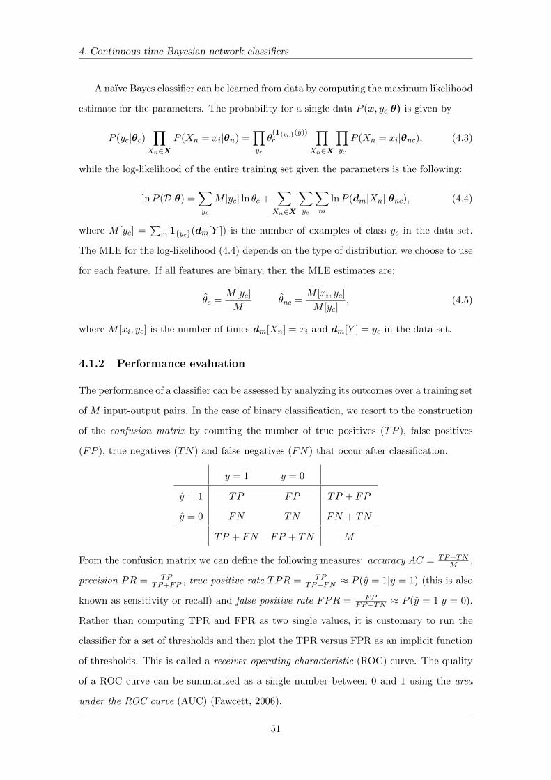
4. Continuous time Bayesian network classifiers
A naıve Bayes classifier can be learned from data by computing the maximum likelihood
estimate for the parameters. The probability for a single data P (x, yc|θ) is given by
P (yc|θc)∏
Xn∈XP (Xn = xi|θn) =
∏yc
θ(1{yc}(y))c
∏Xn∈X
∏yc
P (Xn = xi|θnc), (4.3)
while the log-likelihood of the entire training set given the parameters is the following:
lnP (D|θ) =∑yc
M [yc] ln θc +∑Xn∈X
∑yc
∑m
lnP (dm[Xn]|θnc), (4.4)
where M [yc] =∑
m 1{yc}(dm[Y ]) is the number of examples of class yc in the data set.
The MLE for the log-likelihood (4.4) depends on the type of distribution we choose to use
for each feature. If all features are binary, then the MLE estimates are:
θc =M [yc]
Mθnc =
M [xi, yc]
M [yc], (4.5)
where M [xi, yc] is the number of times dm[Xn] = xi and dm[Y ] = yc in the data set.
4.1.2 Performance evaluation
The performance of a classifier can be assessed by analyzing its outcomes over a training set
of M input-output pairs. In the case of binary classification, we resort to the construction
of the confusion matrix by counting the number of true positives (TP ), false positives
(FP ), true negatives (TN) and false negatives (FN) that occur after classification.
y = 1 y = 0
y = 1 TP FP TP + FP
y = 0 FN TN FN + TN
TP + FN FP + TN M
From the confusion matrix we can define the following measures: accuracy AC = TP+TNM ,
precision PR = TPTP+FP , true positive rate TPR = TP
TP+FN ≈ P (y = 1|y = 1) (this is also
known as sensitivity or recall) and false positive rate FPR = FPFP+TN ≈ P (y = 1|y = 0).
Rather than computing TPR and FPR as two single values, it is customary to run the
classifier for a set of thresholds and then plot the TPR versus FPR as an implicit function
of thresholds. This is called a receiver operating characteristic (ROC) curve. The quality
of a ROC curve can be summarized as a single number between 0 and 1 using the area
under the ROC curve (AUC) (Fawcett, 2006).
51

4. Continuous time Bayesian network classifiers
4.1.3 Bayesian networks as classifiers
Bayesian networks can be used in the context of classification (Friedman et al., 1997).
Specifically, we refer to a Bayesian network classifier as a BN over a set of random variables
X = {X1, . . . , XN} ∪ Y where X1, . . . , XN are the attributes and Y is the class variable.
The graph structure G is such that the class variable has no parents, Pa(Y ) = ∅, and the
attributes can have or not the class variable as parent. Therefore, the problem of learning a
Bayesian network classifier can be rephrased as the problem of learning a general Bayesian
network. In this context we can rewrite equation (4.1) to compute the most probable class
yc as follows:
yc = argmaxyc∈V al(Y )
{P (Y = yc)
∏Xn∈X
P (Xn = xi|Pa(Xn) = pau)
}. (4.6)
The naıve Bayes classifier can be seen as a BN classifier, where each attribute Xn
has the class variable as its unique parent, Pa(Xn) = Y . This classifier has a fixed
structure depicted in Figure 4.1 (a), so no structural learning is required. The graph
structure encodes the assumption that all the attributes are conditionally independent,
given the value of the class. Although this independence assumption is quite restrictive,
this classifier outperformed many sophisticated classifiers (Langley et al., 1992). Different
extensions of this classifier have been introduced to relax this assumption. We mention
the tree augmented naıve Bayes classifier (Friedman et al., 1997), which allows additional
edges between attributes in order to capture some relations among them. Such relations
are restricted to a tree structure as depicted in Figure 4.1 (b).
X X
Y
X1 2 N
(a)
X X
Y
X1 2 N
X 3
(b)
Figure 4.1: The graph structures of common Bayesian network classifiers: (a) naıve Bayes
classifier and (b) tree augmented naıve Bayes classifier.
52
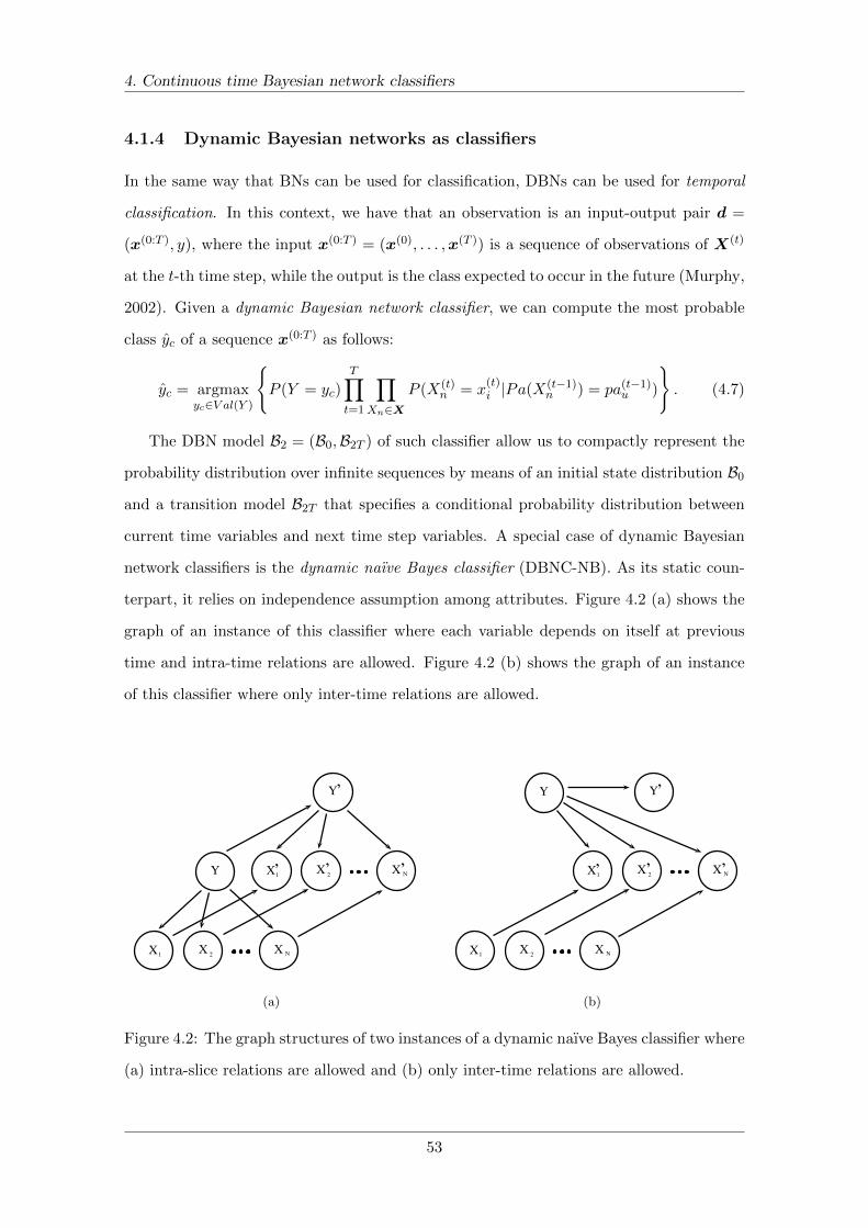
4. Continuous time Bayesian network classifiers
4.1.4 Dynamic Bayesian networks as classifiers
In the same way that BNs can be used for classification, DBNs can be used for temporal
classification. In this context, we have that an observation is an input-output pair d =
(x(0:T ), y), where the input x(0:T ) = (x(0), . . . ,x(T )) is a sequence of observations of X(t)
at the t-th time step, while the output is the class expected to occur in the future (Murphy,
2002). Given a dynamic Bayesian network classifier, we can compute the most probable
class yc of a sequence x(0:T ) as follows:
yc = argmaxyc∈V al(Y )
{P (Y = yc)
T∏t=1
∏Xn∈X
P (X(t)n = x
(t)i |Pa(X(t−1)
n ) = pa(t−1)u )
}. (4.7)
The DBN model B2 = (B0,B2T ) of such classifier allow us to compactly represent the
probability distribution over infinite sequences by means of an initial state distribution B0
and a transition model B2T that specifies a conditional probability distribution between
current time variables and next time step variables. A special case of dynamic Bayesian
network classifiers is the dynamic naıve Bayes classifier (DBNC-NB). As its static coun-
terpart, it relies on independence assumption among attributes. Figure 4.2 (a) shows the
graph of an instance of this classifier where each variable depends on itself at previous
time and intra-time relations are allowed. Figure 4.2 (b) shows the graph of an instance
of this classifier where only inter-time relations are allowed.
X X
Y
X1 2 N
X X
Y
X1 2 N
’
’ ’ ’
(a)
X X
Y
X1 2 N
X X
Y
X1 2 N
’
’ ’ ’
(b)
Figure 4.2: The graph structures of two instances of a dynamic naıve Bayes classifier where
(a) intra-slice relations are allowed and (b) only inter-time relations are allowed.
53

4. Continuous time Bayesian network classifiers
4.2 Continuous time Bayesian network classifiers
The continuous time Bayesian network model has been exploited to perform temporal
classification in which the attributes explicitly evolve in continuous time and not at fixed-
length time step. In this context, we have that an observation is an input-output pair
d = (σ, y), where σ denotes a trajectory that consists of the values of attributes that are
measured in continuous time, while the class y is expected to occur in the future.
4.2.1 Definitions
Continuous time Bayesian networks are translated into a class of supervised classification
models, the class of continuous time Bayesian network classifiers.
Definition 4.1. Continuous time Bayesian network classifier (CTBNC), (Stella and
Amer, 2012). A continuous time Bayesian network classifier is a pair C = (N , P (Y ))
where N is a CTBN model with attribute nodes X = {X1, . . . , XN}, class node Y with
marginal probability P (Y ) on states V al(Y ) = {y1, . . . , yC}, and G is the graph, such that
the following conditions hold: G is connected; Pa(Y ) = ∅, the class variable Y is associated
with a root node; Y is fully specified by P (Y ) and does not depend on time.
From the previous definition it is possible to specify different types of continuous time
Bayesian network classifiers based on the relations among the attribute nodes.
Definition 4.2. Continuous time naıve Bayes (CTBNC-NB), (Stella and Amer, 2012).
A continuous time naıve Bayes is a CTBNC C such that Pa(Xn) = Y, ∀Xn ∈X.
Definition 4.3. Continuous time tree augmented naıve Bayes (CTBNC-TANB), (Stella
and Amer, 2012). A continuous time tree augmented naıve Bayes is a CTBNC C such
that the following conditions hold: Y ∈ Pa(Xn), ∀Xn ∈X and the attribute nodes form a
tree, i.e. ∃ j ∈ {1, . . . , N} : |Pa(Xj)| = 1, while for i 6= j, i = 1, . . . , N : |Pa(Xi)| = 2.
Definition 4.4. Max-k continuous time Bayesian network classifier (CTBNC-Max-k),
(Codecasa and Stella, 2014). A max-k continuous time Bayesian network classifier is a
couple (C, k) where C is a CTBNC such that the number of parents for each attribute node
is bounded by a positive integer k. Formally, the following condition holds: |Pa(Xn)| ≤ k,
∀Xn ∈X and k > 0.
54
4. Continuous time Bayesian network classifiers
4.2.2 Learning
A continuous time Bayesian network classifier C = (N , P (Y )) can be learned on a training
data setD of input-output pair d = (σ, y) using the standard Bayesian learning framework.
For continuous time Bayesian network classifiers we have that the model C consists of three
components. The first is the marginal probability associated with the class node P (Y ).
This marginal probability is independent from the classifier’s structure G and it is not
time-dependent. Given a prior probability on the class node, such as a uniform over
classes, it can be updated by counting the number of examples of a given class in the
available data set. The second is the structure G, as shown in Figure 4.1. The third are
the values of the parameters qG and θG associated with the structure G.
When the graph structure is known, such as for the continuous time naıve Bayes
classifier, the parameter learning of each entry of the intensity matrices is based on log-
likelihood estimation as for the CTBN case shown in (3.19). When the graph structure
is unknown, the dependencies among attributes can be learned using the score-based
approach as for CTBNs presented by Nodelman et al. (2003). For example, the learning
task for a continuous time tree augmented naıve Bayes can be accomplished evaluating the
Bayesian score of different tree structures and searching the structure that has the highest
score. We note that the search space over the tree structures can be done in polynomial
time given a maximum number of possible parents per variable. This search can be easily
performed enumerating each possible tree structure compliant with its definition.
It is noteworthy to mention that the learning goal of a CTBN can be different from that
of a CTBNC. In the CTBN case we would like to describe (or generate) the entire data,
i.e. we are interested in a generative learning. In contrast, in the CTBNC case, we would
like to discriminate between different classes, i.e. we are interested in a discriminative
learning. Generative methods usually maximize the log-likelihood or a score thereof,
whereas discriminative methods focus on maximizing the conditional log-likelihood. In this
regard, Codecasa and Stella (2014) introduced a conditional log-likelihood scoring function
for structural learning of CTBNCs, and they shown that this scoring function combined
with Bayesian parameter estimation outperforms the log-likelihood scoring function, in
particular when the available data is limited.
55
4. Continuous time Bayesian network classifiers
4.2.3 Inference
A continuous time Bayesian network classifier computes the most probable class yc of a
fully observed trajectory σ as follows:
yc = argmaxyc∈V al(Y )
{P (Y = yc)P (σ|Y = yc)} , (4.8)
where P (Y = yc) represents the prior probability of the class yc and P (σ|Y = yc) is the
probability of the fully observed trajectory given the class yc. The latter probability can
be decomposed by temporal intervals of the trajectory as follows:
P (σ|Y = yc) =J∏j=1
P (x[τj−1 : τj)|Y = yc)P (x[x′n][τj : τj+1)|x[τj−1 : τj), Y = yc), (4.9)
where τ0 = 0, . . . , τJ+1 = T are the transition times in the interval [0;T ) for the trajectory.
The term P (x[τj−1 : τj)|Y = yc) represents the probability that X stays in state x during
the time interval [τj−1; τj) given the class yc, while P (x[x′n][τj : τj+1)|x[τj−1 : τj), Y = yc)
represents the probability of a transition of the variable Xn from value xn to the value x′n
(xn 6= x′n) at time τj given the class yc. This latter probability can be written as follows:
P (x[x′n][τj : τj+1)|x[τj−1 : τj), Y = yc) =qxn,x′n|pauqxn|pau
, (4.10)
where qxn,x′n|pau is the parameter associated with the transition of variable Xn from state
xn, in which it was during the interval [τj−1; τj), to state x′n, in which it will be during the
interval [τj ; τj+1), given the state pau of its parents Pa(Xn) during the interval [τj−1; τj),
while qxn|pau is the parameter associated with the variable Xn = xn, in which it was during
the interval [τj−1; τj), given the state pau of its parents Pa(Xn) during the same interval.
The term P (x[τj−1 : τj)|Y = yc) can be further specified for the variable Xn which
transitions at time τj (i.e. xn 6= x′n) and for the variables X \Xn that do not change their
state at time τj (i.e. xn = x′n) as follows:
P (x[τj−1 : τj)|Y = yc) =
exp(−qxn|pau(τj − τj−1)
)if xn = x′n,
qxn|pau exp(−qxn|pau(τj − τj−1)
)if xn 6= x′n.
(4.11)
Equations (4.10) and (4.11), when combined with (4.9), allow us to write:
P (σ|Y = yc) =∏
Xn∈X
∏xn 6=x′n
qxn,x′n|pau∏xn
exp(−qxn|pau(τj − τj−1)
). (4.12)
56
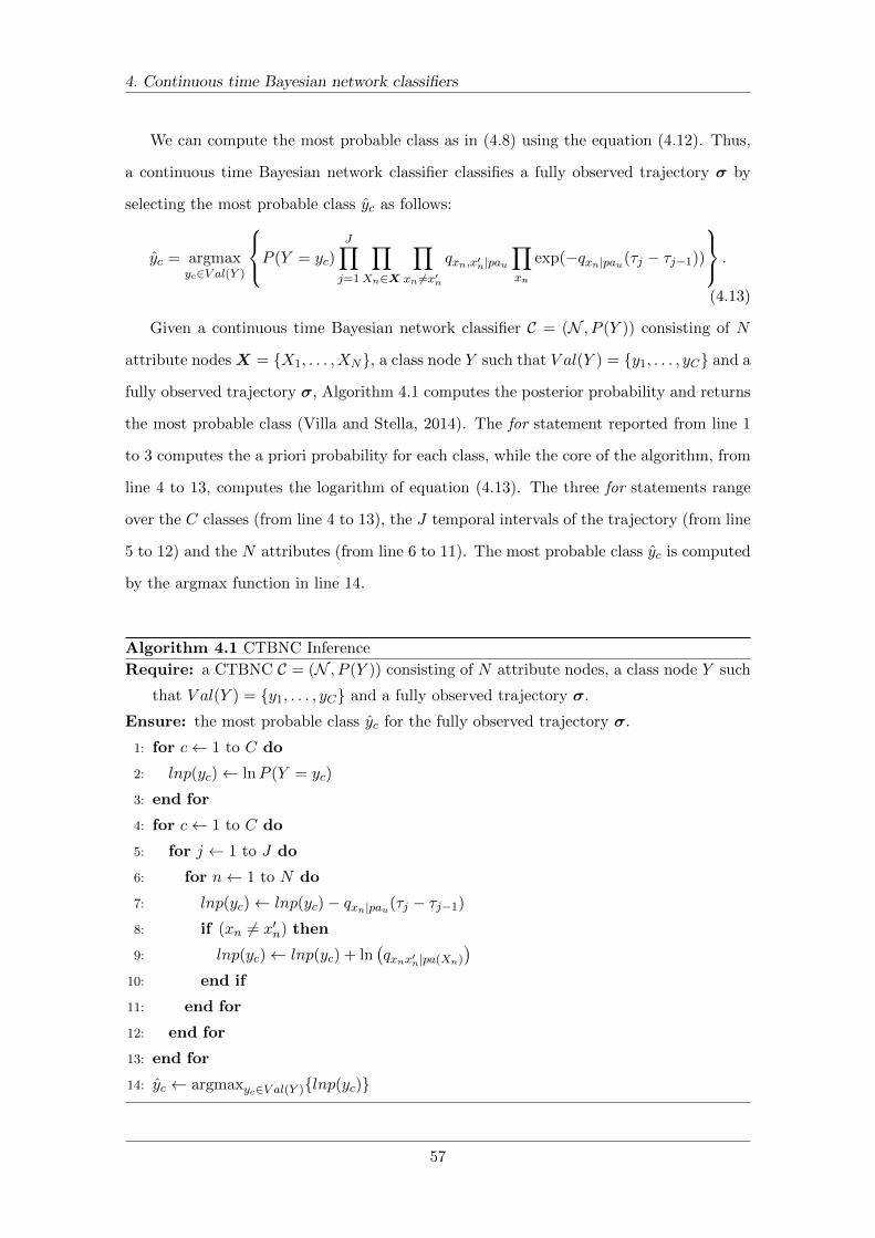
4. Continuous time Bayesian network classifiers
We can compute the most probable class as in (4.8) using the equation (4.12). Thus,
a continuous time Bayesian network classifier classifies a fully observed trajectory σ by
selecting the most probable class yc as follows:
yc = argmaxyc∈V al(Y )
P (Y = yc)J∏j=1
∏Xn∈X
∏xn 6=x′n
qxn,x′n|pau∏xn
exp(−qxn|pau(τj − τj−1))
.
(4.13)
Given a continuous time Bayesian network classifier C = (N , P (Y )) consisting of N
attribute nodesX = {X1, . . . , XN}, a class node Y such that V al(Y ) = {y1, . . . , yC} and a
fully observed trajectory σ, Algorithm 4.1 computes the posterior probability and returns
the most probable class (Villa and Stella, 2014). The for statement reported from line 1
to 3 computes the a priori probability for each class, while the core of the algorithm, from
line 4 to 13, computes the logarithm of equation (4.13). The three for statements range
over the C classes (from line 4 to 13), the J temporal intervals of the trajectory (from line
5 to 12) and the N attributes (from line 6 to 11). The most probable class yc is computed
by the argmax function in line 14.
Algorithm 4.1 CTBNC Inference
Require: a CTBNC C = (N , P (Y )) consisting of N attribute nodes, a class node Y such
that V al(Y ) = {y1, . . . , yC} and a fully observed trajectory σ.
Ensure: the most probable class yc for the fully observed trajectory σ.
1: for c← 1 to C do
2: lnp(yc)← lnP (Y = yc)
3: end for
4: for c← 1 to C do
5: for j ← 1 to J do
6: for n← 1 to N do
7: lnp(yc)← lnp(yc)− qxn|pau(τj − τj−1)
8: if (xn 6= x′n) then
9: lnp(yc)← lnp(yc) + ln(qxnx′n|pa(Xn)
)10: end if
11: end for
12: end for
13: end for
14: yc ← argmaxyc∈V al(Y ){lnp(yc)}
57
4. Continuous time Bayesian network classifiers
4.3 Learning from Big Data
Parameter and structural learning on continuous time Bayesian network classifiers are
challenging tasks when dealing with Big Data. We describe an efficient scalable parallel
algorithm introduced by Villa and Rossetti (2014) for parameter and structural learning
in the case of complete data using the MapReduce framework.
4.3.1 Introduction
The learning algorithms presented so far have a main limitation: when the data size grows
the learning time becomes unacceptable. To overcome this limitation, several paralleliza-
tion alternatives are available. One approach is to use a system with multiple central
processing units (CPUs) and a shared-memory or a distributed-memory cluster made up
of smaller shared-memory systems. This method requires vast resources and specialized
parallel programming expertise. A recent approach consists of using graphics hardware
because the performance increases more rapidly than that of CPUs. Graphics processing
units (GPUs) are designed with a high parallel architecture due to the intrinsic paral-
lel nature of graphics computations. For this reason GPUs are transformed into parallel
computing devices for a wide range of applications (Owens et al., 2007).
A different approach is to use the MapReduce framework (Dean and Ghemawat, 2004).
This framework offers the possibility to implement a parallel application without focusing
on the details of data distribution, load balancing and fault tolerance. MapReduce pro-
grams are expressed as sequences of map and reduce operations performed by the mapper
and the reducer respectively. A mapper takes as input parts of the data set, applies a
function (e.g. a partition of the data) and produces as output key-value pairs, while a
reducer takes as input a list indexed by a key of all corresponding values and applies a
reduction function (e.g. aggregation or sum operations) on the values. Once a reducer
has terminated its work, the next set of mappers can be scheduled. Since a reducer must
wait for all mapper outputs, the synchronization is implicit in the reducer operation, while
fault tolerance is achieved by rescheduling mappers that time out. A free implementation
of MapReduce is Apache Hadoop, which allows the distributed processing of large data
sets across clusters of computers using simple programming models (White, 2009).
58
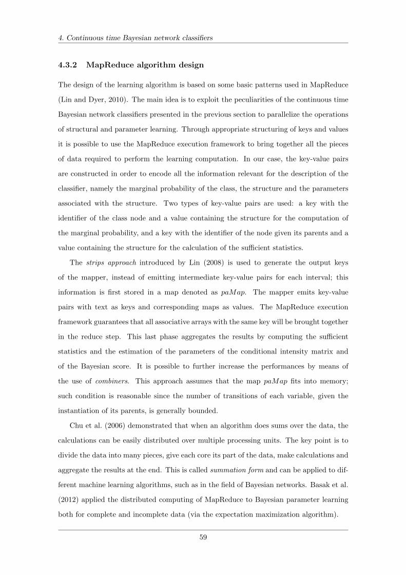
4. Continuous time Bayesian network classifiers
4.3.2 MapReduce algorithm design
The design of the learning algorithm is based on some basic patterns used in MapReduce
(Lin and Dyer, 2010). The main idea is to exploit the peculiarities of the continuous time
Bayesian network classifiers presented in the previous section to parallelize the operations
of structural and parameter learning. Through appropriate structuring of keys and values
it is possible to use the MapReduce execution framework to bring together all the pieces
of data required to perform the learning computation. In our case, the key-value pairs
are constructed in order to encode all the information relevant for the description of the
classifier, namely the marginal probability of the class, the structure and the parameters
associated with the structure. Two types of key-value pairs are used: a key with the
identifier of the class node and a value containing the structure for the computation of
the marginal probability, and a key with the identifier of the node given its parents and a
value containing the structure for the calculation of the sufficient statistics.
The strips approach introduced by Lin (2008) is used to generate the output keys
of the mapper, instead of emitting intermediate key-value pairs for each interval; this
information is first stored in a map denoted as paMap. The mapper emits key-value
pairs with text as keys and corresponding maps as values. The MapReduce execution
framework guarantees that all associative arrays with the same key will be brought together
in the reduce step. This last phase aggregates the results by computing the sufficient
statistics and the estimation of the parameters of the conditional intensity matrix and
of the Bayesian score. It is possible to further increase the performances by means of
the use of combiners. This approach assumes that the map paMap fits into memory;
such condition is reasonable since the number of transitions of each variable, given the
instantiation of its parents, is generally bounded.
Chu et al. (2006) demonstrated that when an algorithm does sums over the data, the
calculations can be easily distributed over multiple processing units. The key point is to
divide the data into many pieces, give each core its part of the data, make calculations and
aggregate the results at the end. This is called summation form and can be applied to dif-
ferent machine learning algorithms, such as in the field of Bayesian networks. Basak et al.
(2012) applied the distributed computing of MapReduce to Bayesian parameter learning
both for complete and incomplete data (via the expectation maximization algorithm).
59

4. Continuous time Bayesian network classifiers
4.3.3 Map, reduce and auxiliary functions
The Map function shown in Algorithm 4.2 counts the transitions and the relative amount
of time in the fully observed trajectory of each variable Xn given the instantiation pau of its
parents Pa(Xn). In the case of structural learning, every possible combination of parents
for each node must be computed subject to the structure constraints, while in the case
of parameter learning the structure G is given as input. The key-value pairs for the class
probability are constructed as textual keys, denoted by CLASS, and values containing
the id of trajectory and the relative class. The key-value pairs for the parameters are
constructed as textual keys encoding the variable name and the names of its parents, i.e.
(Xn|Pa(Xn)), and values containing a two level association of an id corresponding to the
instantiation of parents, another id corresponding to a transition and the count and the
elapsed time of that transition, i.e. < pau, < (xi, xj), (count, time) >>.
Algorithm 4.2 Map
Require: input-output pair (id,σ, y) and structure G (optional).
Ensure: key-value pairs in the forms: if the key is denoted by CLASS, then the value is
< id, y >, while if the key is (Xn|Pa(Xn)), then the value is the map paMap.
1: emit < CLASS, < id, y >>
2: for n← 1 to N do
3: for p← 1 to N do
4: Pa(Xn)← (Y, Xp)
5: if (n = p) then
6: Pa(Xn)← (Y, ∅)7: end if
8: if (AnalyzeParents(Pa(Xn))) then
9: paMap←Map()
10: for j ← 2 to J do
11: paMap← IncrementT(paMap, pa(Xn), (xi, xj), τj − τj−1)
12: paMap← IncrementM(paMap, pa(Xn), (xi, xj), 1)
13: end for
14: emit < (Xn|Pa(Xn)), paMap >
15: end if
16: end for
17: end for
60

4. Continuous time Bayesian network classifiers
The Reduce function shown in Algorithm 4.3 provides the basic elements for the de-
scription of the classifier, namely the class probability and the conditional intensity ma-
trices. This function takes as input key-value pairs where the keys can be CLASS or
(Xn|Pa(Xn)), and the values are collections of data computed by mappers with the same
key, while it produces as output key-value pairs for the model description. The values
are merged into a single map named paMap. If the key is CLASS, then the marginal
probability of the class node is computed, otherwise the Bayesian score and the CIM are
calculated from aggregation of the sufficient statistics.
Algorithm 4.3 Reduce
Require: a key and a list of maps {paMap1, . . . , paMapS}, α and τ hyperparameters.
Ensure: class probability, conditional intensity matrix and Bayesian score.
1: for s← 1 to S do
2: paMap← Merge(paMap, paMaps)
3: end for
4: if (key = CLASS) then
5: marg ← ∅6: for each yc ∈ Values(paMap) do
7: marg(yc)← marg(yc) + 1
8: end for
9: emit < CLASS, marg >
10: else
11: bs← 0
12: for each pau ∈ Keys(paMap) do
13: trMap← paMap [ pau ]
14: T ← ∅,M ← ∅15: for each (xi, xj) ∈ Keys(trMap) do
16: T [xi]← T [xi] + GetT(trMap [ (xi, xj) ])
17: M [xi, xj ]←M [xi, xj ] + GetM(trMap [ (xi, xj) ])
18: end for
19: im← ComputeIM(T, M, α, τ)
20: bs← bs + ComputeBS(T, M, α, τ)
21: emit < CIM,< (key, pau), im >>
22: end for
23: emit < BS, < key, bs >>
24: end if
61

4. Continuous time Bayesian network classifiers
The Map function relies on auxiliary functions in order to compute its output; the
main functions are ComputeIM and ComputeBS. The first function shown in Algorithm 4.4
computes the intensity matrix QXn|pau of the variable Xn given an instantiation pau of its
parents Pa(Xn) by means of counting maps according to the formulas reported in equation
(3.19). The second function shown in Algorithm 4.5 computes the Bayesian score of the
variable Xn given an instantiation pau of its parents Pa(Xn) according to equation (3.28).
Note that the Bayesian score is computed for every parent configuration; the task of the
main function (called driver) is to choose the structure that maximizes the Bayesian score
subject to the model constraints.
Algorithm 4.4 ComputeIM
Require: maps containing the counting values T and M of the node Xn when Pa(Xn) =
pau, α and τ hyperparameters.
Ensure: the intensity matrix QXn|pau for the node Xn when Pa(Xn) = pau.
1: for each (xi, xj) ∈ Transitions(Xn) do
2: if (xi 6= xj) then
3: qxi ←M [xi] + αxiT [xi] + τxi
4: else
5: qxi,xj ←M [xi,xj ] + αxi,xj
T [xi] + τxi
6: end if
7: end for
Algorithm 4.5 ComputeBS
Require: maps containing the counting values T and M of the node Xn when Pa(Xn) =
pau, α and τ hyperparameters.
Ensure: Bayesian score bs of the node Xn when Pa(Xn) = pau.
1: bs← 0
2: for each (xi, xj) ∈ Transitions(Xn) do
3: if (xi 6= xj) then
4: bs← bs+ ln Γ(αxi,xj +M [xi, xj ])− ln Γ(αxi,xj )
5: else
6: bs← bs+ ln Γ(αxi)− ln Γ(αxi +M [xi])
7: bs← bs+ ln Γ(αxi +M [xi] + 1) + (αxi + 1)× ln(τxi)
8: bs← bs− ln Γ(αxi + 1)− (αxi +M [xi] + 1)× ln(τxi + T [xi])
9: end if
10: end for
62

4. Continuous time Bayesian network classifiers
4.3.4 Numerical experiments
The proposed algorithm has been implemented in Java in the Apache Hadoop framework
and its correctness has been tested by comparing the results generated by MapReduce
against a sequential version (Stella and Amer, 2012). Moreover, the software performances
have been tested for the parameter learning of a continuous time naıve Bayes classifier and
for the structural learning of a continuous time tree augmented naıve Bayes. Three types of
experiments have been performed changing the data set size, the number of Hadoop nodes
and the number of attributes. The data set was composed of a text file containing fully
observed trajectories; these trajectories concern transaction data of the foreign exchange
market (Villa and Stella, 2014). The tests were performed using M1 Large instances of
Amazon EMR, while the training and output data were stored in Amazon S3.
In the first experiment, the performance of the MapReduce algorithm has been mea-
sured in the case of parameter learning of a continuous time naıve Bayes classifier. This
algorithm used 1 Master instance and 5 Core instances against the sequential algorithm
using only one instance. The data set consisted of 1 binary class variable and 6 binary
attributes, while the training set size has been varied from 25K to 200K trajectories with
steps of 25K. Figure 4.3 (a) illustrates the learning time compared to the data set size.
This picture shows the time taken by the algorithms and the regression lines which inter-
polate the data points. Intuitively, the increase of the size of the training samples leads to
increased training time because the MapReduce implementation has a computational over-
head, which with few data led to bad performance. Figure 4.3 (b) illustrates the speedup
between the sequential and MapReduce algorithms (real) and the speedup between the
two regression lines (theoretical). As the data size increases, the speedup grows quickly
at the beginning, while it becomes more stable when the data size is already big enough
(e.g. with 200K trajectories we have a speedup of about 3).
In the second experiment, the number of Hadoop nodes has been varied to assess
the parallel performance of the MapReduce algorithm in the case of parameter learning
using the same training set of 200K trajectories. Figure 4.3 (c) shows the changes in the
training time using different numbers of Hadoop nodes from 5 to 25 with steps of 5 nodes.
As expected, increasing the number of Hadoop nodes significantly reduces the learning
time, even if this reduction is not equal to the ratio between the number of nodes.
63
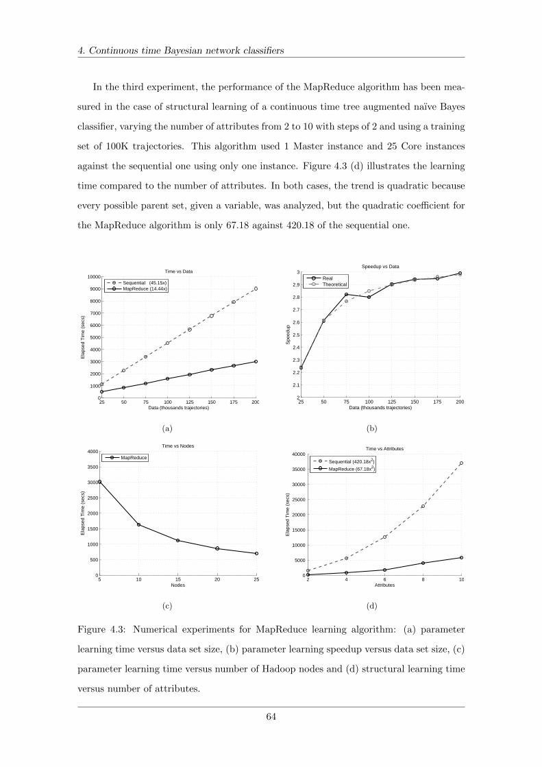
4. Continuous time Bayesian network classifiers
In the third experiment, the performance of the MapReduce algorithm has been mea-
sured in the case of structural learning of a continuous time tree augmented naıve Bayes
classifier, varying the number of attributes from 2 to 10 with steps of 2 and using a training
set of 100K trajectories. This algorithm used 1 Master instance and 25 Core instances
against the sequential one using only one instance. Figure 4.3 (d) illustrates the learning
time compared to the number of attributes. In both cases, the trend is quadratic because
every possible parent set, given a variable, was analyzed, but the quadratic coefficient for
the MapReduce algorithm is only 67.18 against 420.18 of the sequential one.
25 50 75 100 125 150 175 2000
1000
2000
3000
4000
5000
6000
7000
8000
9000
10000
Ela
psed
Tim
e (s
ecs)
Data (thousands trajectories)
Time vs Data
Sequential (45.15x)MapReduce (14.44x)
(a)
25 50 75 100 125 150 175 2002
2.1
2.2
2.3
2.4
2.5
2.6
2.7
2.8
2.9
3
Spe
edup
Data (thousands trajectories)
Speedup vs Data
RealTheoretical
(b)
5 10 15 20 250
500
1000
1500
2000
2500
3000
3500
4000
Ela
psed
Tim
e (s
ecs)
Nodes
Time vs Nodes
MapReduce
(c)
2 4 6 8 10 0
5000
10000
15000
20000
25000
30000
35000
40000
Ela
psed
Tim
e (s
ecs)
Attributes
Time vs Attributes
Sequential (420.18x2)
MapReduce (67.18x2)
(d)
Figure 4.3: Numerical experiments for MapReduce learning algorithm: (a) parameter
learning time versus data set size, (b) parameter learning speedup versus data set size, (c)
parameter learning time versus number of Hadoop nodes and (d) structural learning time
versus number of attributes.
64
4. Continuous time Bayesian network classifiers
4.4 The FX forecasting problem
We present how it is possible to exploit continuous time Bayesian network classifiers for
the prediction of foreign exchange (FX) spot rates introduced by Villa and Stella (2014).
The performance of an instance of these classifiers is analyzed and compared to that of
the dynamic Bayesian network by using real tick by tick FX rates. The achieved results
based on different metrics show clearly a predictive power of these models for FX rates at
high frequencies. These results also show that the proposed classifier is more effective and
more efficient than dynamic Bayesian network classifier.
4.4.1 Financial context
High frequency financial data, made available by electronic order driven markets, has
started a revolution on data processing and statistical modeling. This revolution forces
quantitative analysts to cope with challenging theoretical and computational problems.
Indeed, high frequency financial data has to take into account micro structure effects
which cannot be appreciated when using longer time intervals (Treleaven et al., 2013).
We focus on high frequency transaction data from the FX market that is the largest and
most liquid financial market. Its rapid growth over the last few years has been facilitated by
the wider use of electronic trading at both levels, i.e. broker-dealer markets and customer
markets deployed through on line trading platforms. The FX market is affected by many
correlated economical, political and even psychological factors that make its forecasting
a hard task. Researchers and practitioners have been striving for an explanation of the
movement of exchange rates. It has long been known that structural models fail to predict
exchange rates at short term horizons (Chinn and Meese, 1995; Kilian and Taylor, 2003).
The basic question to be answered is whether it is possible or not to forecast the
behavior of an economic variable over a short time interval. The efficient market hypothesis
(EMH), a fundamental pillar of modern economics (Fama, 1965), states that forecasting
is not possible. The weak form of this hypothesis asserts that the asset price reflects all
of the information that can be obtained from its history. Accordingly to the EMH, the
asset price follows a random walk, and thus the best prediction of the future asset price is
given by its current price. Thus, the movement of the price of an asset is unpredictable.
65
4. Continuous time Bayesian network classifiers
A common myth of traders is that there is a certain predictability of market dynam-
ics. Many efforts have been devoted to proving or disproving the EMH with several works
rejecting it with specific reference to intraday data. Zhang (1999) exploited conditional
entropy to show that even the most competitive markets are not strictly efficient; Baviera
et al. (2000) rejected the random walk hypothesis for high frequency FX returns and pro-
posed a Markovian model which reproduces the available information of the financial series;
Renner et al. (2001) found evidence of Markov properties for high frequency exchange rate
data; Baviera et al. (2002) found anti-persistent Markov behavior of log-price fluctuations
in high frequency FX rates, which in principle allows the possibility of a statistical forecast;
Ohira et al. (2002) found that there is a rather particular conditional probability structure
in high frequency FX data; Tanaka-Yamawaki (2003) observed stability of a Markovian
structure in high frequency FX data; recently, Shmilovici et al. (2009) tested the EMH
using a variable order Markov model for twelve pairs of intraday currency exchange rates
for one year series with different time granularity. The authors found that intraday cur-
rency exchange rates are predictable above the random guess. These empirical evidences
reveal that some predictability of high frequency FX rates exists.
The specialized literature describes FX forecasting techniques based on different as-
sumptions and methods. Traditional parametric forecasting methods, such as auto re-
gressive conditional heteroskedastic models and their extensions, were used to capture the
salient features of the exchange rate volatility (Vilasuso, 2002). Recent developments in
artificial intelligence and machine learning techniques, together with a continuously in-
creasing availability of computational power, have allowed nonparametric models to be
applied to FX forecasting. The techniques used in the FX rates forecasting range from
artificial neural networks (Yao and Tan, 2000; Leung et al., 2000; Yu et al., 2007), support
vector machines (Kamruzzaman et al., 2003), to genetic algorithms (Dempster and Jones,
2001). In the recent literature, hybrid models have also been proposed. Ince and Trafalis
(2006) combined parametric and nonparametric techniques to achieve better performance
for daily exchange rate forecasting. Gradojevic (2007) combined artificial neural networks
and fuzzy logic controllers to obtain the optimal daily currency trading rules. Kablan and
Ng (2011) introduced an adaptive neuro-fuzzy inference system for financial trading which
learns to predict FX price movements of tick by tick data.
66
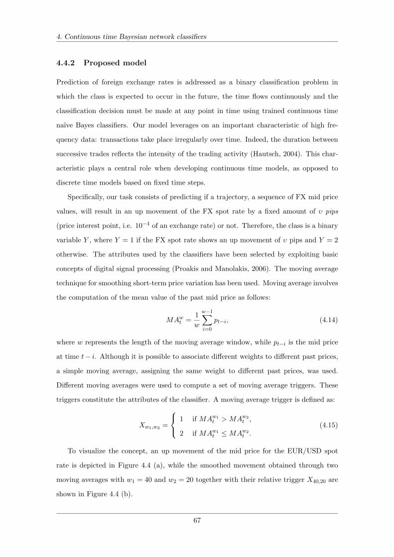
4. Continuous time Bayesian network classifiers
4.4.2 Proposed model
Prediction of foreign exchange rates is addressed as a binary classification problem in
which the class is expected to occur in the future, the time flows continuously and the
classification decision must be made at any point in time using trained continuous time
naıve Bayes classifiers. Our model leverages on an important characteristic of high fre-
quency data: transactions take place irregularly over time. Indeed, the duration between
successive trades reflects the intensity of the trading activity (Hautsch, 2004). This char-
acteristic plays a central role when developing continuous time models, as opposed to
discrete time models based on fixed time steps.
Specifically, our task consists of predicting if a trajectory, a sequence of FX mid price
values, will result in an up movement of the FX spot rate by a fixed amount of υ pips
(price interest point, i.e. 10−4 of an exchange rate) or not. Therefore, the class is a binary
variable Y , where Y = 1 if the FX spot rate shows an up movement of υ pips and Y = 2
otherwise. The attributes used by the classifiers have been selected by exploiting basic
concepts of digital signal processing (Proakis and Manolakis, 2006). The moving average
technique for smoothing short-term price variation has been used. Moving average involves
the computation of the mean value of the past mid price as follows:
MAwt =1
w
w−1∑i=0
pt−i, (4.14)
where w represents the length of the moving average window, while pt−i is the mid price
at time t− i. Although it is possible to associate different weights to different past prices,
a simple moving average, assigning the same weight to different past prices, was used.
Different moving averages were used to compute a set of moving average triggers. These
triggers constitute the attributes of the classifier. A moving average trigger is defined as:
Xw1,w2 =
1 if MAw1t > MAw2
t ,
2 if MAw1t ≤MAw2
t .(4.15)
To visualize the concept, an up movement of the mid price for the EUR/USD spot
rate is depicted in Figure 4.4 (a), while the smoothed movement obtained through two
moving averages with w1 = 40 and w2 = 20 together with their relative trigger X40,20 are
shown in Figure 4.4 (b).
67
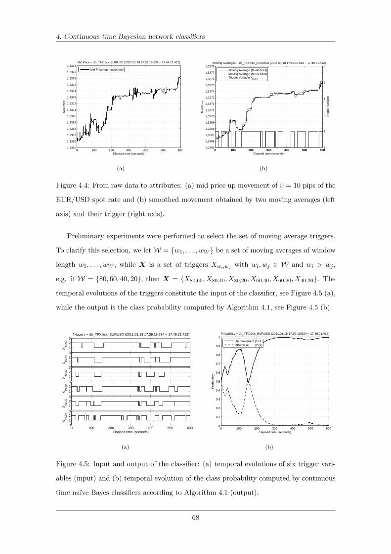
4. Continuous time Bayesian network classifiers
0 100 200 300 400 500 6001,3365
1,3366
1,3367
1,3368
1,3369
1,3370
1,3371
1,3372
1,3373
1,3374
1,3375
1,3376
1,3377
1,3378
Elapsed time (seconds)
Mid
Pric
eMid Price − db_TFX.tick_EURUSD (2011.01.18 17:39:19.534 − 17:49:21.412)
Mid Price (up movement)
(a)
0 100 200 300 400 500 6001,3365
1,3366
1,3367
1,3368
1,3369
1,3370
1,3371
1,3372
1,3373
1,3374
1,3375
1,3376
1,3377
1,3378
Mid
Pric
e
Elapsed time (seconds)
Moving Averages − db_TFX.tick_EURUSD (2011.01.18 17:39:19.534 − 17:49:21.412)
0 100 200 300 400 500 6001
2
3
4
5
6
Trig
ger
Var
iabl
e
Moving Average (M=40 ticks)Moving Average (M=20 ticks)Trigger Variable X
40,20
(b)
Figure 4.4: From raw data to attributes: (a) mid price up movement of υ = 10 pips of the
EUR/USD spot rate and (b) smoothed movement obtained by two moving averages (left
axis) and their trigger (right axis).
Preliminary experiments were performed to select the set of moving average triggers.
To clarify this selection, we let W = {w1, . . . , wW } be a set of moving averages of window
length w1, . . . , wW , while X is a set of triggers Xwi,wj with wi, wj ∈ W and wi > wj ,
e.g. if W = {80, 60, 40, 20}, then X = {X80,60, X80,40, X80,20, X60,40, X60,20, X40,20}. The
temporal evolutions of the triggers constitute the input of the classifier, see Figure 4.5 (a),
while the output is the class probability computed by Algorithm 4.1, see Figure 4.5 (b).
123
Triggers − db_TFX.tick_EURUSD (2011.01.18 17:39:19.534 − 17:49:21.412)
X80
,60
123
X80
,40
123
X80
,20
123
X60
,40
123
X60
,20
0 100 200 300 400 500 6000123
Elapsed time (seconds)
X40
,20
(a)
0 100 200 300 400 500 6000
0.1
0.2
0.3
0.4
0.5
0.6
0.7
0.8
0.9
1
Elapsed time (seconds)
Pro
babi
lity
Probability − db_TFX.tick_EURUSD (2011.01.18 17:39:19.534 − 17:49:21.412)
Up movement (Y=1)Otherwise (Y=2)
(b)
Figure 4.5: Input and output of the classifier: (a) temporal evolutions of six trigger vari-
ables (input) and (b) temporal evolution of the class probability computed by continuous
time naıve Bayes classifiers according to Algorithm 4.1 (output).
68

4. Continuous time Bayesian network classifiers
4.4.3 Benchmarking
The dynamic naıve Bayes classifier was used as benchmark, where the parameter learning
task has been performed with the algorithm described by Murphy (2002), while inference
has been performed by using the BK algorithm introduced by Boyen and Koller (1998).
Figure 4.6 shows the evolution of the posterior probability associated with the class
variable Y (up movement of υ = 10 pips) for the EUR/USD spot rate computed by the
dynamic classifier. Note that the continuous time classifier allows to obtain the posterior
probability of the class variable at each point in time; conversely, the same does not occur
for the dynamic classifier, which provides probability values at discrete time points (∆t)
computed via the approximate inference algorithm. It is important to note that, for large
values of the time slice ∆t, the dynamic classifier simply cannot capture the transition
dynamics accurately enough to converge to competitive performance.
Villa and Stella (2014) compared the computational effort required for learning and
inference with respect to the number of trajectories and they concluded that the continuous
time classifier is very efficient versus the dynamic classifier. In fact, the time required for
learning the continuous time classifier with 1,000 trajectories is 8 times less than that
required for a dynamic classifier with ∆t = 60 secs, while the time required for inference
is 182 times less then that required by its discrete counterpart with ∆t = 10 secs.
0 100 200 300 400 500 6000
0.1
0.2
0.3
0.4
0.5
0.6
0.7
0.8
0.9
1Probability − db_TFX.tick_EURUSD (2011.01.18 17:39:19.534 − 17:49:21.412)
Elapsed Time (seconds)
Pro
babi
lity
Up movement (Y=1)Otherwise (Y=2)
(a)
0 100 200 300 400 500 6000
0.1
0.2
0.3
0.4
0.5
0.6
0.7
0.8
0.9
1
Elapsed time (seconds)
Pro
babi
lity
Probability − db_TFX.tick_EURUSD (2011.01.18 17:39:19.534 − 17:49:21.412)
Up movement (Y=1)Otherwise (Y=2)
(b)
Figure 4.6: Class probability evolutions of a mid price up movement of υ = 10 pips using
trained dynamic naıve Bayes classifiers with (a) ∆t = 10 secs and (b) ∆t = 60 secs.
69
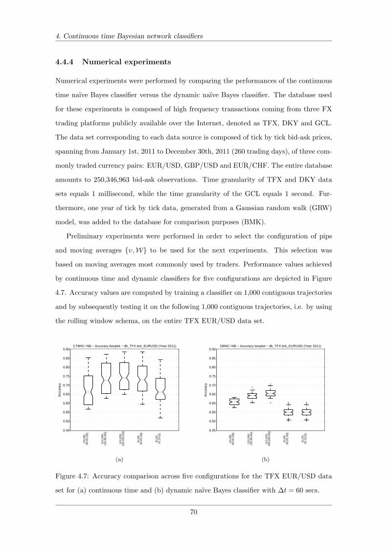
4. Continuous time Bayesian network classifiers
4.4.4 Numerical experiments
Numerical experiments were performed by comparing the performances of the continuous
time naıve Bayes classifier versus the dynamic naıve Bayes classifier. The database used
for these experiments is composed of high frequency transactions coming from three FX
trading platforms publicly available over the Internet, denoted as TFX, DKY and GCL.
The data set corresponding to each data source is composed of tick by tick bid-ask prices,
spanning from January 1st, 2011 to December 30th, 2011 (260 trading days), of three com-
monly traded currency pairs: EUR/USD, GBP/USD and EUR/CHF. The entire database
amounts to 250,346,963 bid-ask observations. Time granularity of TFX and DKY data
sets equals 1 millisecond, while the time granularity of the GCL equals 1 second. Fur-
thermore, one year of tick by tick data, generated from a Gaussian random walk (GRW)
model, was added to the database for comparison purposes (BMK).
Preliminary experiments were performed in order to select the configuration of pips
and moving averages {υ,W} to be used for the next experiments. This selection was
based on moving averages most commonly used by traders. Performance values achieved
by continuous time and dynamic classifiers for five configurations are depicted in Figure
4.7. Accuracy values are computed by training a classifier on 1,000 contiguous trajectories
and by subsequently testing it on the following 1,000 contiguous trajectories, i.e. by using
the rolling window schema, on the entire TFX EUR/USD data set.
0.45
0.50
0.55
0.60
0.65
0.70
0.75
0.80
0.85
0.90
{10,
{80,
60
,40,
20}}
{10,
{160
,
120,
80,4
0}}
{10,
{200
,
150,
100,
50}}
{5,{
40,
30
,20,
10}}
{5,{
20,
15
,10,
5}}
Acc
urac
y
CTBNC−NB − Accuracy boxplot − db_TFX.tick_EURUSD (Year 2011)
(a)
0.45
0.50
0.55
0.60
0.65
0.70
0.75
0.80
0.85
0.90
{10,
{80,
60
,40,
20}}
{10,
{160
,
120,
80,4
0}}
{10,
{200
,
150,
100,
50}}
{5,{
40,
30
,20,
10}}
{5,{
20,
15
,10,
5}}
Acc
urac
y
DBNC−NB − Accuracy boxplot − db_TFX.tick_EURUSD (Year 2011)
(b)
Figure 4.7: Accuracy comparison across five configurations for the TFX EUR/USD data
set for (a) continuous time and (b) dynamic naıve Bayes classifier with ∆t = 60 secs.
70
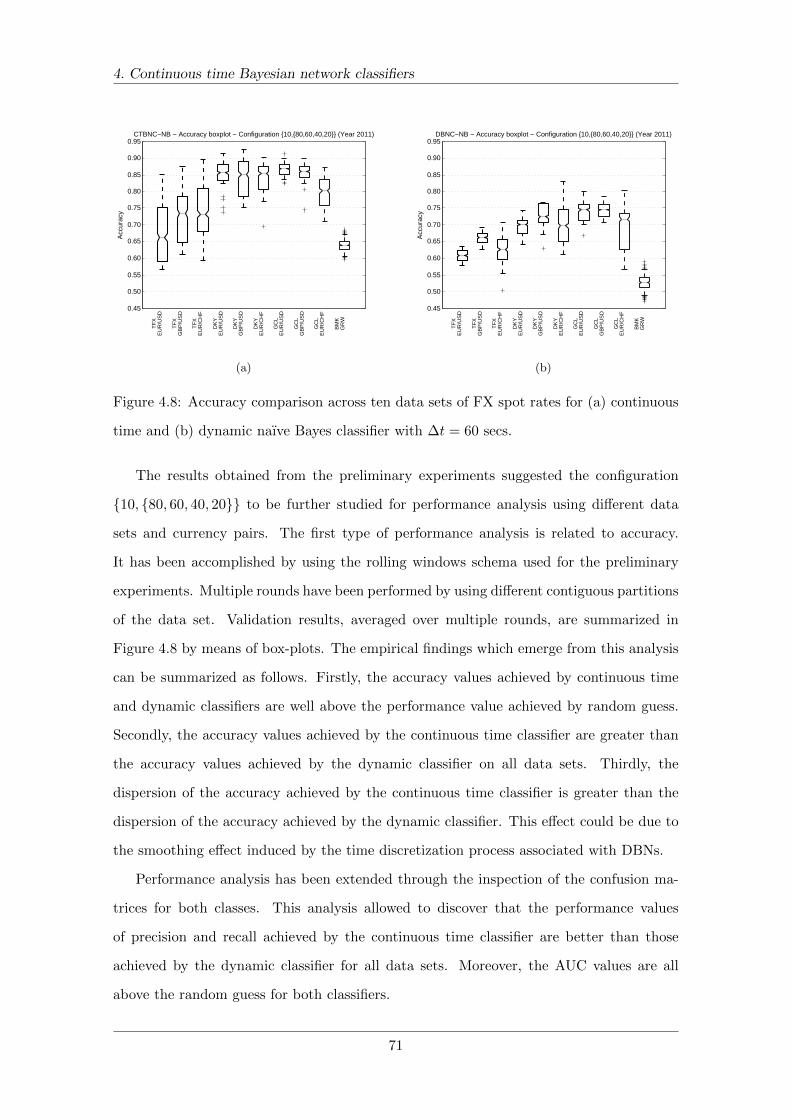
4. Continuous time Bayesian network classifiers
0.45
0.50
0.55
0.60
0.65
0.70
0.75
0.80
0.85
0.90
0.95
TF
X
EU
R/U
SD
TF
X
GB
P/U
SD
TF
X
EU
R/C
HF
DK
Y
EU
R/U
SD
DK
Y
GB
P/U
SD
DK
Y
EU
R/C
HF
GC
L
E
UR
/US
D
GC
L
G
BP
/US
D
GC
L
E
UR
/CH
F
BM
K
GR
W
Acc
urac
y
CTBNC−NB − Accuracy boxplot − Configuration {10,{80,60,40,20}} (Year 2011)
(a)
0.45
0.50
0.55
0.60
0.65
0.70
0.75
0.80
0.85
0.90
0.95
TF
X
EU
R/U
SD
TF
X
GB
P/U
SD
TF
X
EU
R/C
HF
DK
Y
EU
R/U
SD
DK
Y
GB
P/U
SD
DK
Y
EU
R/C
HF
GC
L
E
UR
/US
D
GC
L
G
BP
/US
D
GC
L
E
UR
/CH
F
BM
K
GR
W
Acc
urac
y
DBNC−NB − Accuracy boxplot − Configuration {10,{80,60,40,20}} (Year 2011)
(b)
Figure 4.8: Accuracy comparison across ten data sets of FX spot rates for (a) continuous
time and (b) dynamic naıve Bayes classifier with ∆t = 60 secs.
The results obtained from the preliminary experiments suggested the configuration
{10, {80, 60, 40, 20}} to be further studied for performance analysis using different data
sets and currency pairs. The first type of performance analysis is related to accuracy.
It has been accomplished by using the rolling windows schema used for the preliminary
experiments. Multiple rounds have been performed by using different contiguous partitions
of the data set. Validation results, averaged over multiple rounds, are summarized in
Figure 4.8 by means of box-plots. The empirical findings which emerge from this analysis
can be summarized as follows. Firstly, the accuracy values achieved by continuous time
and dynamic classifiers are well above the performance value achieved by random guess.
Secondly, the accuracy values achieved by the continuous time classifier are greater than
the accuracy values achieved by the dynamic classifier on all data sets. Thirdly, the
dispersion of the accuracy achieved by the continuous time classifier is greater than the
dispersion of the accuracy achieved by the dynamic classifier. This effect could be due to
the smoothing effect induced by the time discretization process associated with DBNs.
Performance analysis has been extended through the inspection of the confusion ma-
trices for both classes. This analysis allowed to discover that the performance values
of precision and recall achieved by the continuous time classifier are better than those
achieved by the dynamic classifier for all data sets. Moreover, the AUC values are all
above the random guess for both classifiers.
71

4. Continuous time Bayesian network classifiers
The ROC curves associated with continuous time and dynamic classifier have been
constructed when predicting the class Y = 1 (up movement of 10 pips) for the EUR/USD
data sets; these curves are depicted in Figure 4.9. This picture shows the fraction of
true up movements out of the total number of up movements (i.e. true positive rate)
against the fraction of false up movements out of the total number of down movements
(i.e. false positive rate) for different probability thresholds. The ROC curves have been
computed by vertical averaging, i.e. by taking vertical samples of the ROC curves for fixed
false positive rates and by averaging the corresponding true positive rates, as suggested by
Fawcett (2006). The ROC curves remark the above random predictions for both classifiers
with some differences within classifiers and data sets.
It is important to note that the high values of accuracy reached do not imply that
trading profitability has been achieved. For this purpose we highlight at least two relevant
aspects. Firstly, the issue of early classification and the study of the trade-off between
earliness and accuracy should be considered, see Xing et al. (2009, 2010). Secondly, a dy-
namic decision strategy which generates trading signals based on the probability evolutions
should be designed, such as in Bertsimas et al. (2003).
0 0.1 0.2 0.3 0.4 0.5 0.6 0.7 0.8 0.9 10
0.1
0.2
0.3
0.4
0.5
0.6
0.7
0.8
0.9
1
Tru
e P
ositi
ve R
ate
False Positive Rate
CTBNC−NB − ROC (Y=1) − Configuration {10,{80,60,40,20}} − (Year 2011)
TFX EUR/USDDKY EUR/USDGCL EUR/USDRandom
(a)
0 0.1 0.2 0.3 0.4 0.5 0.6 0.7 0.8 0.9 10
0.1
0.2
0.3
0.4
0.5
0.6
0.7
0.8
0.9
1
Tru
e P
ositi
ve R
ate
False Positive Rate
DBNC−NB − ROC (Y=1) − Configuration {10,{80,60,40,20}} − (Year 2011)
TFX EUR/USDDKY EUR/USDGCL EUR/USDRandom
(b)
Figure 4.9: ROC curves using the configuration {10, {80, 60, 40, 20}} for EUR/USD data
sets associated with (a) continuous time naıve Bayes classifier and (b) dynamic naıve Bayes
classifier with ∆t = 60 secs.
72
4. Continuous time Bayesian network classifiers
4.5 Discussion
After a brief introduction about the basic concepts of classification, we have presented
the continuous time Bayesian network classifiers and addressed the learning and inference
tasks in the case of complete data. We have discussed a MapReduce algorithm for learning
in the context of Big Data. Different experiments have shown that this algorithm scales
well in the distributed processing environment. The performances can be improved if the
algorithms were executed on a huge amount of data using many computational nodes.
The advantage of MapReduce depends not only on the size of the input data, but also on
the structure of the graph and on the number of states of the variables. In fact, it is not
necessary to maintain the counting map in memory, which can be critical in large networks
with many states. Furthermore, the algorithm we presented provides a base case for the
extension of Big Data learning of continuous time Bayesian networks in both complete
and incomplete data. The Big Data phenomenon is well known in finance. In recent
years, we have seen a rapid growth of high frequency data as a result of the advancements
in computational and mass storage technology. This has led to a high demand of new
approaches to data processing and statistical analysis. In the last part of this chapter,
we have presented a straightforward application of these classifiers to the FX forecasting
problem to natively deal with unevenly spaced time data, i.e. the main characteristic of
high frequency data. Extensive experimental tests have shown a strong predictive power
of these models and a higher efficiency compared to dynamic Bayesian network classifiers.
73
Chapter 5
Non-stationary continuous time
Bayesian networks
Continuous time Bayesian networks have been extended to the structural non-stationary
class of models where the underlying data generating processes are non homogeneous. We
start this chapter by discussing the reasons for non-stationary modeling and the common
approaches developed in the literature. We continue introducing the definition of non-
stationary continuous time Bayesian networks and their structural learning framework.
We move on to describe the structural learning algorithms in three different settings based
on the available knowledge. We finish by presenting numerical experiments performed to
evaluate the correct reconstruction of the graphs sequence provided by these algorithms.
5.1 Stationary versus non-stationary modeling
The identification of relationships and statistical dependencies between components in
multivariate time-series concerns many research domains such as biology, finance, traffic
engineering and neurology, to mention just a few areas. In biology, for example, it is clear
that knowing the gene regulatory network allows to understand complex biological mech-
anisms ruling the cell. In such a context, Bayesian networks (Friedman et al., 2000; Segal
et al., 2005), dynamic Bayesian networks (Zou and Conzen, 2005; Vinh et al., 2012) and
continuous time Bayesian networks (Acerbi and Stella, 2014) have been used to reconstruct
transcriptional regulatory networks from gene expression data.
74
5. Non-stationary continuous time Bayesian networks
While stationarity is a reasonable assumption in many situations, there are cases where
this is no longer acceptable. Indeed, in the last few years, researchers from different disci-
plines have started to be interested in representing relationships and dependencies which
change over time. In particular, they have been interested in analyzing the temporal evo-
lution of genetic networks (Ahmed and Xing, 2009; Lebre et al., 2010), neural information
flow networks (Smith et al., 2006) and dependence structure among financial markets dur-
ing the global financial crisis (Durante and Dunson, 2014). While there have been various
efforts to adapt Bayesian networks (Nielsen and Nielsen, 2008) and undirected graphical
models (Xuan and Murphy, 2007) to non-stationary domains, relaxing the non homo-
geneity assumption in dynamic Bayesian networks has become popular in recent years.
Specifically, structural learning of dynamic Bayesian networks has been proposed as a
principled method for identifying the conditional independence structure in multivariate
time-series data (Robinson and Hartemink, 2010).
5.1.1 Structural and parameter non-stationary models
According to Robinson and Hartemink (2010), there are two possible types of models that
learn non-stationarities: structural non-stationary and parameter non-stationary.
Structural non-stationary approaches explicitly model the presence of statistical de-
pendencies between variables and allow them to appear and disappear over time, e.g. they
construct directed or undirected networks whose edges change over time. Some examples
are temporal exponential random graph model, where a structural evolutionary process is
modeled with a set of features between adjacent network structures (Hanneke and Xing,
2006) and non-stationary dynamic Bayesian network, an extension of the DBN model
where the structure is evolving over time (Robinson and Hartemink, 2009).
Modeling short time-series segments with separate networks could lead to inflated in-
ference uncertainty. Parameter non-stationary approaches try to overcome this issue by
modeling the evolution of parameters over time while keeping the structure fixed. Some
examples are the switching state-space model that represents a piecewise-stationary exten-
sion of a linear dynamic system (Ghahramani and Hinton, 2000) and the non-stationary
continuous dynamic Bayesian network, a non-stationary DBN for continuous data where
only the parameters are allowed to vary over time (Grzegorczyk and Husmeier, 2009).
75
5. Non-stationary continuous time Bayesian networks
5.1.2 Dynamic Bayesian networks in non-stationary domains
Dynamic Bayesian networks have been extended to deal with non-stationary domains as
they allow inter-time relationships to be modeled and, under certain assumptions (such
as parameter independence and conjugate prior), the parameters can be integrated out in
closed form in the likelihood function. The common approaches are the following.
Robinson and Hartemink (2009) introduced the non-stationary dynamic Bayesian net-
work model, a structural non-stationary DBN where a Markov chain Monte Carlo (MCMC)
sampling algorithm is used to learn the structures from time-series data. Their learning
framework is based on the Bayesian-Dirichlet equivalent metric, while the change-points
are common to the whole network, i.e. they cannot vary from node to node.
Grzegorczyk and Husmeier (2009) proposed a parameter non-stationary DBN for con-
tinuous data, called non-stationary continuous dynamic Bayesian network, where the num-
bers and locations of the change-points are sampled from the posterior distribution. Their
learning framework is based on Bayesian Gaussian equivalent (BGe) metric and the pat-
terns of non-stationarity are node-specific, thereby providing extra model flexibility.
Song et al. (2009) introduced the time-varying dynamic Bayesian network model, a
structural non-stationary DBN for continuous data, where they used a kernel reweighted l1-
regularized autoregressive approach for learning the sequence of networks. Their approach
is node-specific, as they estimated the edges for each node separately and then joined these
edges to form the overall network.
Lebre et al. (2010) proposed the auto regressive time varying model where a structural
non-stationary DBN is used to model the interactions between variables, while a reversible
jump MCMC (RJMCMC) is used for inferring simultaneously the times when the network
changes and the resulting network topologies. Their method is based on the Bayesian linear
regression model which avoids the need for data discretization.
Dondelinger et al. (2013) proposed a model for continuous data based on a piecewise
homogeneous dynamic Bayesian network. This model is structural non-stationary, as it
allows the network structure to change over time, and node-specific, as it allows different
penalties for changing edges and non-edges in the network. The values of the parame-
ters are sampled from a posterior distribution computed via an improved version of the
RJMCMC algorithm.
76
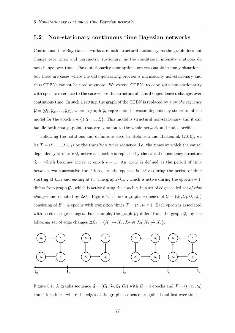
5. Non-stationary continuous time Bayesian networks
5.2 Non-stationary continuous time Bayesian networks
Continuous time Bayesian networks are both structural stationary, as the graph does not
change over time, and parametric stationary, as the conditional intensity matrices do
not change over time. These stationarity assumptions are reasonable in many situations,
but there are cases where the data generating process is intrinsically non-stationary and
thus CTBNs cannot be used anymore. We extend CTBNs to cope with non-stationarity
with specific reference to the case where the structure of causal dependencies changes over
continuous time. In such a setting, the graph of the CTBN is replaced by a graphs sequence
G = (G1,G2, . . . ,GE), where a graph Ge represents the causal dependency structure of the
model for the epoch e ∈ {1, 2, . . . , E}. This model is structural non-stationary and it can
handle both change-points that are common to the whole network and node-specific.
Following the notations and definitions used by Robinson and Hartemink (2010), we
let T = (t1, . . . , tE−1) be the transition times sequence, i.e. the times at which the causal
dependency structure Ge active at epoch e is replaced by the causal dependency structure
Ge+1 which becomes active at epoch e + 1. An epoch is defined as the period of time
between two consecutive transitions, i.e. the epoch e is active during the period of time
starting at te−1 and ending at te. The graph Ge+1, which is active during the epoch e+ 1,
differs from graph Ge, which is active during the epoch e, in a set of edges called set of edge
changes and denoted by ∆Ge. Figure 5.1 shows a graphs sequence of G = (G1,G2,G3,G4)
consisting of E = 4 epochs with transition times T = (t1, t2, t3). Each epoch is associated
with a set of edge changes. For example, the graph G2 differs from the graph G1 by the
following set of edge changes ∆G1 = {X3 → X2, X2 6→ X3, X1 6→ X2}.
X1 X2
X3X4
X1 X2
X3X4
X1 X2
X3X4
X1 X2
X3X4
t0 t1 t 2 t3t 4
Figure 5.1: A graphs sequence G = (G1,G2,G3,G4) with E = 4 epochs and T = (t1, t2, t3)
transition times, where the edges of the graphs sequence are gained and lost over time.
77

5. Non-stationary continuous time Bayesian networks
5.2.1 Definition
Non-stationary continuous time Bayesian networks allow each node to have its own se-
quence of parents sets, each parent set being active at a given epoch. Therefore, we need to
introduce the concept of homogeneous interval H(X) = (h1, . . . , hM ) associated with node
X, which is defined as the union of consecutive epochs during which the same parent set
Pa(X) is active for the node X. It is important to note that in the case where each epoch
is associated with a different parent set, then M is equal to E. We can now introduce the
definition of such a model.
Definition 5.1. (Structural) non-stationary continuous time Bayesian network (nsCTBN),
(Stella and Villa, 2014). Let X be a set of random variables X1, . . . , XN . Each X has a fi-
nite domain of values V al(X) = {x1, . . . , xI}. A non-stationary continuous time Bayesian
network Nns = (B,Mns) over X consists of two components: the first is an initial dis-
tribution P 0X , specified as a Bayesian network B over X, the second is a non-stationary
continuous time transition model Mns specified as:
• a sequence of directed (possibly cyclic) graphs G = (Ge)Ee=1 whose nodes are X1, . . . , XN
and E is the number of epochs;
• a conditional intensity matrix, QX|PaG(X),H(X), ∀X ∈ X, where PaG(X) denotes
the parents sets of X in G and H(X) denotes the intervals associated with X.
In this case, a conditional intensity matrix QX|PaG(X),H(X) consists of a set of intensity
matrices, one intensity matrix for each configuration pau of the parent set Pa(X) which
is active during the interval hm ∈ H(X). Thus, an intensity matrix is defined as follows:
QX|pau,hm =
−qx1|pau,hm qx1,x2|pau,hm . qx1,xI |pau,hm
qx2,x1|pau,hm −qx2|pau,hm . qx2,xI |pau,hm
. . . .
qxI ,x1|pau,hm qxI ,x2|pau,hm . −qxI |pau,hm
,
where qxi|pau,hm =∑
xj 6=xi qxi,xj |pau,hm . The off-diagonal elements of this matrix can be
thought as the “instantaneous probability” of transitioning from xi to xj when Pa(X) =
pau in the interval H(X) = hm, while the diagonal elements can be seen as “instantaneous
probability” of leaving state xi when Pa(X) = pau in the interval H(X) = hm.
78
5. Non-stationary continuous time Bayesian networks
Learning a nsCTBN from a fully observed data set D can be done using the standard
Bayesian learning framework developed for CTBNs. In such a framework, we must specify
a prior probability distribution P (G) over the graphs sequence G and, for each possible
sequence, a density measure over possible values of the parameters qG and θG . Once
the prior P (G) and the likelihood P (qG ,θG |G) are given, we can compute the marginal
likelihood P (D|G) and thus the Bayesian score can be evaluated.
It is important to note that we are focused on recovering the graphs sequence and not
on detecting possible changes of the parameters. In fact, we identify non-stationarity in
the parameters of the model, i.e. the elements of the CIMs, that are significant enough to
result in structural changes of the graph. Thus, we assume that other changes are small
enough not to alter the graph structure.
5.2.2 Prior probability over the graphs sequence
Unlike the standard learning framework for CTBNs which involves a single graph G, the
prior over the nsCTBN’s structure P (G) concerns an entire graphs sequence. If the number
of epochs E is given, then we can write the prior over the nsCTBN’s structure as follows:
P (G|E) = P (G1, . . . ,GE |E)
= P (G1,∆G1, . . . ,∆GE−1|E)
= P (G1)P (∆G1, . . . ,∆GE−1|E). (5.1)
In this case, we have to define a probability distribution for the initial network P (G1)
and a probability distribution for the set of edge changes P (∆G1, . . . ,∆GE−1|E). If some
knowledge about particular edges or overall topology is available for the initial network,
then we can use an informative prior P (G1), otherwise we can resort to a uniform distribu-
tion. As in the BNs case, P (G1) must satisfy the structure modularity assumption (2.17).
The role of the prior on the surviving structures is crucial, since it allows the graphs not
to vary dramatically between adjacent epochs. Therefore, the graphs are selected placing
some assumptions on the ways by which the edges change through graphs. For example,
Robinson and Hartemink (2010) assume that the graph evolves smoothly over time and
they use a truncated geometric prior on the number of changes for each each set ∆Ge.
79

5. Non-stationary continuous time Bayesian networks
5.2.3 Prior probability over parameters
The prior over parameters P (qG ,θG |G, T ) is selected in order to satisfy the following
standard assumptions: independence between the sets of parameters characterizing the
exponential and the multinomial distributions (3.12), parameter modularity (2.19) and
parameter independence. For nsCTBNs, the latter assumption is divided into three com-
ponents: global, interval and local parameter independence.
The global parameter independence asserts that the parameters associated with each
node in a graphs sequence are independent, so the prior over parameters can be decom-
posed by variable X as follows:
P (qG ,θG |G, T ) =∏X∈X
P (qX|PaG(X),H(X),θX|PaG(X),H(X)|G, T ). (5.2)
The interval parameter independence states that the parameters associated with each
interval of the active parents for each node are independent, so the parameters associated
with each X and its parents Pa(X) are decomposable by interval hm ∈ H(X) as follows:
P (qX|PaG(X),H(X),θX|PaG(X),H(X)|G, T ) =∏hm
P (qX|PaG(X),hm ,θX|PaG(X),hm |G, T ).
(5.3)
The local parameter independence states that the parameters associated with each state
of a variable in an interval are independent, thus the parameters associated with each X
in an interval hm ∈ H(X) are decomposable by parent configuration pau as follows:
P (qX|PaG(X),hm ,θX|PaG(X),hm |G, T ) =∏pau
∏xi
P (qxi|pau,hm ,θxi|pau,hm |G, T ). (5.4)
As for CTBNs, we use a Dirichlet distribution as the prior for the parameters of the
multinomial distribution and a gamma distribution as the prior for the parameters of the
exponential distribution, while the sufficient statistics are modified as follows:
• T [xi|pau, hm]: the amount of time spent in state X = xi while Pa(X) = pau in
interval H(X) = hm;
• M [xi, xj |pau, hm]: the number of transitions from X = xi to X = xj while Pa(X) =
pau in interval H(X) = hm.
The number of times the variable X leaves state xi while its parents Pa(X) are in state
pau during interval H(X) = hm is M [xi|pau, hm] =∑
xj 6=xiM [xi, xj |pau, hm].
80

5. Non-stationary continuous time Bayesian networks
5.2.4 Marginal likelihood
Given the graphs sequence G and the transition times T , the marginal likelihood P (D|G, T )
of the data set D, given the graphs sequence and the transition times, can be computed
in closed form using the priors and the sufficient statistics previously defined. To derive
the Bayesian-Dirichlet equivalent metric for nsCTBNs, we make the same assumptions as
those for CTBNs. In this case, the parameter independence assumption is divided into
global (5.2), interval (5.3) and local (5.4). Therefore, the marginal likelihood becomes:
P (D|G, T ) =∏X∈X
MLX(qX|PaG(X),H(X)|D)×MLX(θX|PaG(X),H(X)|D), (5.5)
where the marginal likelihood of q in equation (5.5) is:
∏hm
∏pau
∏xi
Γ(αxi|pau,hm +M [xi|pau, hm] + 1
) (τxi|pau,hm
)(αxi|pau,hm+1)
Γ(αxi|pau,hm + 1
) (τxi|pau,hm + T [xi|pau, hm]
)(αxi|pau,hm+M [xi|pau,hm]+1), (5.6)
while the marginal likelihood of θ in equation (5.5) is:
∏hm
∏pau
∏xi=xj
Γ(αxi|pau,hm
)Γ(αxi|pau,hm +M [xi|pau, hm]
) × ∏xi 6=xj
Γ(αxi,xj |pau,hm +M [xi, xj |pau, hm]
)Γ(αxi,xj |pau,hm
) .
(5.7)
It is important to note that for nsCTBNs, pseudocounts α as well as imaginary amount
of time τ are associated with each interval. This aspect requires a careful choice in order
not to be too biased towards these values in the case when small intervals are analyzed. A
possible correction is to weight the CTBN’s hyperparameters by a quantity proportional
to the time interval width (hm − hm−1). Thus, the nsCTBN’ hyperparameters can be
written as follows:
αxi,xj |pau,hm = αxi,xj |pau ×(hm − hm−1)
hM, τxi|pau,hm = τxi|pau ×
(hm − hm−1)
hM, (5.8)
where hM represents the total time. If we want to control the parameter priors using only
two hyperparameters α and τ , we can use the uniform BDe for nsCTBNs. In this case, the
hyperparameters defined in (5.8) are divided by the number U of possible configurations
of the parents of node X times the cardinality I of the domain of X, as follows:
αxi,xj |pau,hm =α
U × I ×(hm − hm−1)
hM, τxi|pau,hm =
τ
U × I ×(hm − hm−1)
hM. (5.9)
81
5. Non-stationary continuous time Bayesian networks
5.3 Structural learning settings
The structural learning of nsCTBNs is addressed as the problem of selecting the graphs
sequence G and the corresponding parameters values which maximize the Bayesian score.
To efficiently solve this problem, i.e. to search for the optimal graphs sequence G∗, we need
to decompose the Bayesian score by variable as done for CTBNs. However, for nsCTBNs,
the score decomposition depends on the level of knowledge we have on the transition
times. In particular, we take into account the same learning settings as those introduced
and analyzed by Robinson and Hartemink (2010): known transitions times, known number
of epochs and unknown number of epochs.
5.3.1 Known transition times
If the transition times T are known, then the prior probability over the graphs sequence
P (G) decomposes as in equation (5.1). Therefore, from equation (5.5) we obtain that the
marginal likelihood decomposes by variable X, while the Bayesian score is the following:
BS(G : D, T ) = lnP (G1) + lnP (∆G1, . . . ,∆GE−1|T ) (5.10)
+∑X∈X
lnMLX(qX|PaG(X),H(X)|D) + lnMLX(θX|PaG(X),H(X)|D).
In such a setting the structural leaning problem of a non-stationary continuous time
Bayesian network consists of finding the graph G1 active during the first epoch (e = 1), the
E − 1 sets of edge changes ∆G1, . . . ,∆GE−1 together with the corresponding parameters
values which maximize the Bayesian score defined in equation (5.10). If some knowledge
about the structure of the initial graph G1 is available, then we can use an informative prior
for P (G1) which must satisfy the structure modularity property (2.17). On the contrary,
if no prior knowledge is available, then a uniform distribution is used.
The graphs G2, . . . ,GE are selected by making assumptions on the ways by which the
edges change over continuous time. Thus, we have to define prior for P (∆G1, . . . ,∆GE−1|T ).
We make the same assumption as the one made in Robinson and Hartemink (2010). In
particular, we assume that the structural component of the non-stationary continuous
time Bayesian network, i.e. the graphs sequence G = (G1,G2, . . . ,GE), evolves smoothly
over continuous time.
82
5. Non-stationary continuous time Bayesian networks
In such a case, we use a truncated geometric distribution with parameter p = 1 −
exp(−λc) on the number of parents’ changes occurring at transition time e+ 1:
ce =∑X∈X
c(PaGe(X), PaGe+1(X)), (5.11)
where c counts the number of edge changes between two parent sets. If the edge changes
∆Ge are assumed to be mutually independent, then the probability for the edge changes
through subsequent epochs can be written as follows:
P (∆G1, . . . ,∆GE−1|T ) =
E−1∏e=1
(1− exp(−λc))(exp(−λc))ce1− (exp(−λc))cmax+1
∝E−1∏e=1
(exp(−λc))ce , (5.12)
where cmax is the truncation term. Thus, the Bayesian score (5.10) decomposes by variable:
BS(G : D, T ) =∑X∈X
lnP (Pa(X) = PaG1(X))− λcE−1∑e=1
c(PaGe(X), PaGe+1(X))
+ lnMLX(q,θX|PaG(X),H(X)|D), (5.13)
where we grouped together the marginal likelihoods of q and θ. Note that the number
of parents’ changes for each epoch penalizes the Bayesian score, and thus it discourages
sudden variations, while the parameter λc regulates the impacts of these changes.
5.3.2 Known number of epochs
If the transition times T are unknown, then the Bayesian score associated with the
nsCTBN can be written as follows:
BS(G, T : D) = lnP (G, T ) + lnP (D|G, T ). (5.14)
In such a setting, to decompose this Bayesian score, we assume that the joint probability
P (G, T ) of the evolution of the structural component of the nsCTBNs and the transition
times can be decomposed into two independent components: P (G) and P (T ). Therefore,
the Bayesian score (5.14) can be written as follows:
BS(G, T : D) = lnP (G) + lnP (T ) + lnP (D|G, T ). (5.15)
If the number of epochs E is known, then the prior probability P (G) over the graphs
sequence G decomposes as in equation (5.1). Therefore, also in this setting, a truncated
geometric distribution can be used on the number of parents’ changes occurring at each
transition time, as we made in the known transition time setting.
83
5. Non-stationary continuous time Bayesian networks
Any choice for P (T ) can be made to include prior knowledge about the set of transition
times. However, if no information is available, then we use a uniform prior on P (T )
implying that all possible values of transition times are equally likely for a given number
E of epochs. Therefore, in the known number of epochs setting, the Bayesian score can
be decomposed by variable as follows:
BS(G, T : D) = lnP (T )
+∑X∈X
lnP (Pa(X) = PaG1(X))− λcE−1∑e=1
c(PaGe(X), PaGe+1(X))
+ lnMLX(q,θX|PaG(X),H(X)|D). (5.16)
5.3.3 Unknown number of epochs
If both the transition times T and the number of epochs E are unknown, then they must
be estimated through the Bayesian score. To accomplish this task, we exploit what we
introduced for the known transition times and the known number of epochs settings. In
particular, we assume that the structure of the non-stationary continuous time Bayesian
network evolves smoothly over continuous time. Such an assumption is incorporated by
using a truncated geometric distribution with parameter p = 1− exp(−λe) on the number
of epochs. Following what we presented in the known transition times setting, the Bayesian
score can be obtained by subtracting the parameter λe times the number of epochs E.
Therefore, in this setting, the Bayesian score decomposes by variable as follows:
BS(G, T : D) = lnP (T )− λeE
+∑X∈X
lnP (Pa(X) = PaG1(X))− λcE−1∑e=1
c(PaGe(X), PaGe+1(X))
+ lnMLX(q,θX|PaG(X),H(X)|D). (5.17)
Note that this version of the Bayesian score contains two parameters, namely λc and
λe, which encode our prior belief about the structure of the non-stationary continuous
time Bayesian network. Specifically, the parameter λc regulates our prior belief about the
smoothness of the edge changes (e.g. encouraging or discouraging few edge changes per
epoch), while the parameter λe regulates our prior belief about the number of epochs (e.g.
encouraging or discouraging the creation of few epochs).
84
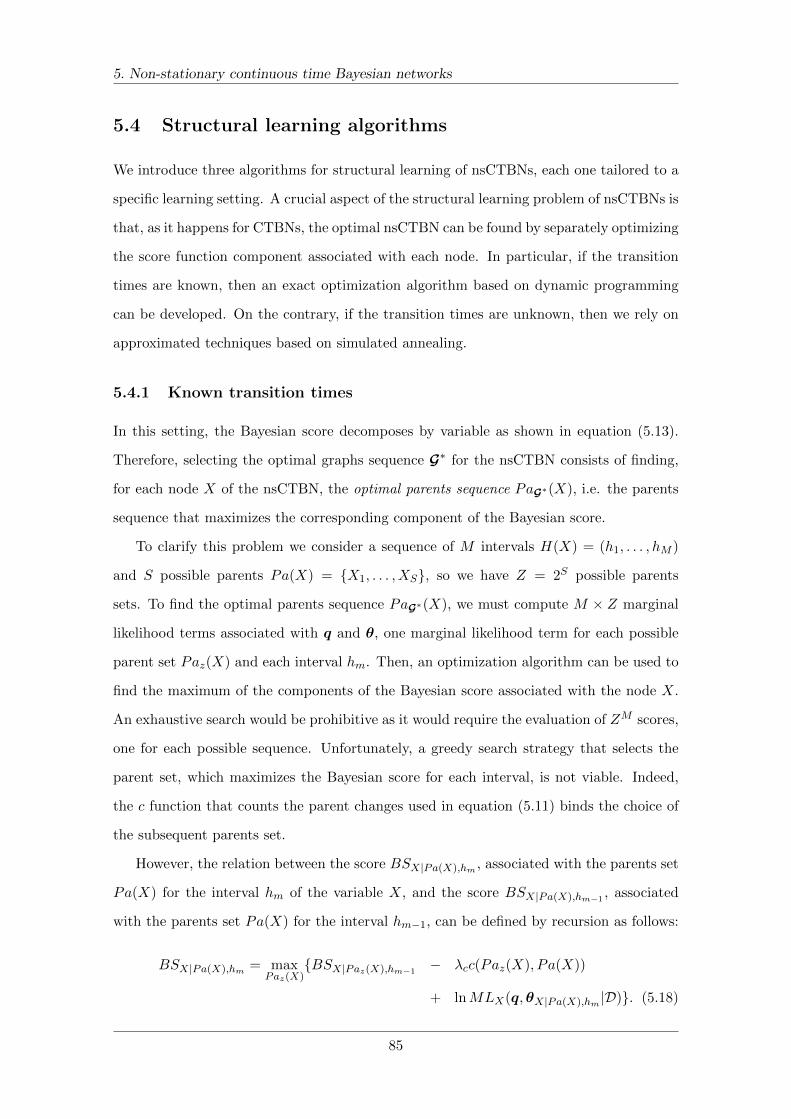
5. Non-stationary continuous time Bayesian networks
5.4 Structural learning algorithms
We introduce three algorithms for structural learning of nsCTBNs, each one tailored to a
specific learning setting. A crucial aspect of the structural learning problem of nsCTBNs is
that, as it happens for CTBNs, the optimal nsCTBN can be found by separately optimizing
the score function component associated with each node. In particular, if the transition
times are known, then an exact optimization algorithm based on dynamic programming
can be developed. On the contrary, if the transition times are unknown, then we rely on
approximated techniques based on simulated annealing.
5.4.1 Known transition times
In this setting, the Bayesian score decomposes by variable as shown in equation (5.13).
Therefore, selecting the optimal graphs sequence G∗ for the nsCTBN consists of finding,
for each node X of the nsCTBN, the optimal parents sequence PaG∗(X), i.e. the parents
sequence that maximizes the corresponding component of the Bayesian score.
To clarify this problem we consider a sequence of M intervals H(X) = (h1, . . . , hM )
and S possible parents Pa(X) = {X1, . . . , XS}, so we have Z = 2S possible parents
sets. To find the optimal parents sequence PaG∗(X), we must compute M × Z marginal
likelihood terms associated with q and θ, one marginal likelihood term for each possible
parent set Paz(X) and each interval hm. Then, an optimization algorithm can be used to
find the maximum of the components of the Bayesian score associated with the node X.
An exhaustive search would be prohibitive as it would require the evaluation of ZM scores,
one for each possible sequence. Unfortunately, a greedy search strategy that selects the
parent set, which maximizes the Bayesian score for each interval, is not viable. Indeed,
the c function that counts the parent changes used in equation (5.11) binds the choice of
the subsequent parents set.
However, the relation between the score BSX|Pa(X),hm , associated with the parents set
Pa(X) for the interval hm of the variable X, and the score BSX|Pa(X),hm−1, associated
with the parents set Pa(X) for the interval hm−1, can be defined by recursion as follows:
BSX|Pa(X),hm = maxPaz(X)
{BSX|Paz(X),hm−1− λcc(Paz(X), Pa(X))
+ lnMLX(q,θX|Pa(X),hm |D)}. (5.18)
85

5. Non-stationary continuous time Bayesian networks
The equation (5.18) is exploited by the dynamic programming technique shown in
Algorithm 5.1. This algorithm takes as input the marginal likelihoods of q and θ for each
interval and parents set, i.e. MLX(q,θX|Pa(X),hm |D), the prior probability about the
initial parent set, i.e. P (Pa(X) = PaGh1 (X)), the number of parents’ changes, i.e. the
c function used in equation (5.11), and the parameter λc. It ensures the optimal parents
sequence PaG∗(X) for the node X and its relative optimal Bayesian score.
The core of Algorithm 5.1 is the computation of the M × Z score matrix, denoted by
SC, through the dynamic programming recursion. In the first interval h1 (m = 1), for
1 ≤ z ≤ Z, this recursion is defined as follows:
SC[1, z] = lnP (Paz(X) = PaGh1 (X)) + lnMLX(q,θX|Paz(X),h1 |D), (5.19)
for the subsequent intervals hm (m = 2, . . . ,M), the recursion is defined as follows:
SC[m, z] = max1≤w≤Z
{SC[m− 1, w]− λcc(Paw(X), Paz(X)) + lnMLX(q,θX|Paz(X),hm |D)
}(5.20)
After filling the SC matrix, the value maxz{SC[M, z]} is the optimal Bayesian score, while
the optimal parents sequence is reconstructed backwards from M to 1 by using the IN
matrix. The cost of computing the dynamic programming recursion is O(M ×Z2), which
is polynomial for a fixed number of parents S.
The problem of selecting the optimal parents sequence PaG∗(X) has an interesting
graph representation. Indeed, it is possible to create a graph whose nodes are associated
with marginal likelihoods of q and θ for interval hm and parents set Paz(X), while each
node associated with interval hm is linked with all the nodes associated with interval
hm+1. Each arc is associated with a weight computed as the difference between the
marginal likelihoods of q and θ in the interval hm for the parents set Paz(X) and the cost
of switching from the parents set of the interval hm−1 to the parents set of the interval hm.
To conclude the graph representation, two special nodes are added to represent the start
and the end of the optimal parents sequence. Such a graph does not have cycles, thus the
selection of the optimal parents sequence for each node can be reduced to a longest path
problem from the start node to the end node over a directed acyclic graph, and thus it
can be solved using either dynamic or linear programming.
86

5. Non-stationary continuous time Bayesian networks
Learning a nsCTBN model can be summarized in four steps: i) compute the suffi-
cient statistics over the data set according to the given transitions times; ii) calculate the
marginal likelihoods and fill the MLX matrix for each variable; iii) run Algorithm 5.1 for
each variable in order to get the optimal parents sequence; iv) collect the optimal parents
sequence of each variable and compute the corresponding CIMs using the sufficient statis-
tics already computed in i). If we allow the intervals to differ from the transition times,
i.e. they can be obtained as one of all the possible unions of transition times, then we have
to repeat the learning procedure for all the possible E × (E − 1)/2 cases. Fortunately, we
can speed up this computation. In fact, the sufficient statistics can be aggregated through
intervals; in such a way we read the data set once, while the precomputed marginal like-
lihoods can be stored and reused for the same intervals. Moreover, the computations can
be performed in parallel for each variable.
Algorithm 5.1 LearnKTTX
Require: matrix containing the marginal likelihoods of q and θ MLX[M,Z], vector
containing the prior probability about the initial parent set PR[Z], matrix containing
the number of parents’ changes C[Z,Z] and the parameter for the parent changes λc.
Ensure: score matrix SC[M,Z] and index matrix IN [M,Z].
1: Initialize SC[m, z]← −∞, IN [m, z]← 0.
2: for m← 1, . . . ,M do
3: for z ← 1, . . . , Z do
4: if (m = 1) then
5: SC[m, z]← lnMLX[m, z] + lnPR[z]
6: else
7: for w ← 1, . . . , Z do
8: score← SC[m− 1, w] + lnMLX[m, z]− λcC[w, z]
9: if (score > SC[m, z]) then
10: SC[m, z]← score
11: IN [m, z]← w
12: end if
13: end for
14: end if
15: end for
16: end for
87

5. Non-stationary continuous time Bayesian networks
5.4.2 Known number of epochs
In this setting, we know the number of epochs, but the transition times are not given, so
we cannot directly apply Algorithm 5.1 to solve the structural learning problem. However,
once a tentative allocation T of the transition times is given, we can apply Algorithm 5.1
to obtain the optimal solution. This optimal solution assumes that T is not too different
from the true and unknown transition times T .
We developed and applied the simulated annealing (SA) algorithm (Kirkpatrick et al.,
1983; Cerny, 1985) to find the allocation T ∗ which is as close as possible to T . We give
a brief description of this technique. SA is a stochastic algorithm that attempts to find
the global optimum of a given function f(x) where x represents the current solution,
also referred to as state. SA is an iterative algorithm that, at each step, samples a new
state x′ according to some proposal distribution P ′(·|x). Once the new state x′ has been
proposed, the following quantity is computed α = exp(−f(x)−f(x′)
CT
), where CT denotes
the computational temperature. SA accepts the proposed state x′ with probability equal
to min{1, α}, thus moving from state x to state x′, otherwise the current state x does not
change. SA always accepts any proposed state x′ where f(x′) > f(x), while it accepts
the proposed state x′ when f(x′) < f(x) with probability α.
The computational temperature CT reduces over iterations according to a cooling
schedule. It has been shown that if one cools sufficiently slowly, then the algorithm will
provably find the global optimum (Kirkpatrick et al., 1983). However, it is not clear how to
implement this in practice. An approach is to use an exponential cooling schedule defined
as follows: CTk = CT0 × ζk, where CT0 represents the initial temperature typically set to
1.0, ζ is the cooling rate usually set to be close to 0.8 and k is the current step (Murphy,
2012). The best cooling schedule is difficult to determine: if it cools too quickly, then it
risks getting stuck in a local optimum, while if cools too slowly, then it wastes time. This
is the main drawback of simulated annealing (Bertsimas and Tsitsiklis, 1993).
In the case of nsCTBNs the state x is the tentative allocation T , while the function
f(x) to be optimized is the Bayesian score (5.16). Algorithm 5.2 solves the structural
learning problem in the known number of epochs setting for a given node by ensuring the
optimal tentative allocation T ∗ and its Bayesian score. It takes as input the sufficient
statistics, the parameters used to run Algorithm 5.1 and the parameters regarding the SA
88
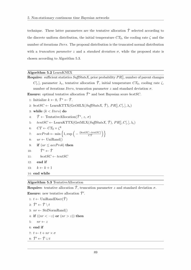
5. Non-stationary continuous time Bayesian networks
technique. These latter parameters are the tentative allocation T selected according to
the discrete uniform distribution, the initial temperature CT0, the cooling rate ζ and the
number of iterations Iters. The proposal distribution is the truncated normal distribution
with a truncation parameter z and a standard deviation σ, while the proposed state is
chosen according to Algorithm 5.3.
Algorithm 5.2 LearnKNEX
Require: sufficient statistics SuffStatsX, prior probability PR[], number of parent changes
C[, ], parameter λc, tentative allocation T , initial temperature CT0, cooling rate ζ,
number of iterations Iters, truncation parameter z and standard deviation σ.
Ensure: optimal tentative allocation T ∗ and best Bayesian score bestSC.
1: Initialize k ← 0, T ∗ ← T .
2: bestSC ← LearnKTTX(GetMLX(SuffStatsX, T ), PR[], C[, ], λc)
3: while (k < Iters) do
4: T ← TentativeAllocation(T ∗, z, σ)
5: tentSC ← LearnKTTX(GetMLX(SuffStatsX, T ), PR[], C[, ], λc)
6: CT ← CT0 × ζk
7: accProb← min{
1, exp(− (bestSC−tentSC)
CT
)}8: ur ← UniRand()
9: if (ur ≤ accProb) then
10: T ∗ ← T11: bestSC ← tentSC
12: end if
13: k ← k + 1
14: end while
Algorithm 5.3 TentativeAllocation
Require: tentative allocation T , truncation parameter z and standard deviation σ.
Ensure: new tentative allocation T ′.1: t← UniRandDiscr(T )
2: T ′ ← T \ t3: nr ← StdNormRand()
4: if ((nr < −z) or (nr > z)) then
5: nr ← z
6: end if
7: t← t+ nr × σ8: T ′ ← T ∪ t
89
5. Non-stationary continuous time Bayesian networks
5.4.3 Unknown number of epochs
In this setting, the number of epochs is unknown, thus the structural learning algorithm
must be able to change the number of epochs, as well as the corresponding transition
times. Also in this case, we used the simulated annealing technique, where the state x
is the tentative allocation T and the function f(x) to be optimized is the Bayesian score
shown in equation (5.17). The cooling schedule is set to be the same as the one used for
the known number of epochs setting.
The proposal distribution differs from the one of the previous case as it uses two
additional operators, namely split and merge. The split operator allows to split a given
interval [tm; tm+1) into two subintervals [tm; t) and [t; tm+1), where tm, tm+1 ∈ T . The
merge operator allows to merge contiguous intervals [tm−1; tm) and [tm; tm+1) to form the
wider interval [tm−1; tm+1), where tm−1, tm, tm+1 ∈ T . The new state x′ is obtained by
sampling the number of epochs changes ec from a multinoulli distribution with parameters
(p1, p2, p3), where p1 represents the probability that the current number of epochs |T | is
decreased by one, p3 represents the probability that the current number of epochs |T | is
increased by one, and p2 represents the probability that the current number of epochs |T |
does not change. If ec is equal to 2, then the Algorithm 5.2 is invoked. If ec is equal to 1,
then the merge operator is applied before running the Algorithm 5.2. If ec is equal to 3,
then the split operator is applied before running the Algorithm 5.2.
Algorithm 5.4 solves the structural learning problem in the unknown number of epochs
setting for a given node X by ensuring the optimal tentative allocation T ∗ and its corre-
sponding Bayesian score. This algorithm is basically the same as the one in the known
number of epochs settings, but it uses Algorithm 5.5 to perform the two additional opera-
tors. Specifically, the split operator is implemented as follows: a time interval [tm; tm+1),
selected according to a discrete uniform distribution, is evenly splitted to obtain two equal
width intervals, i.e. [tm; t) and [t; tm+1) where t is the mid point in [tm; tm+1). The merge
operator is implemented as follows: a transition time tm belonging to T is sampled ac-
cording to a discrete uniform distribution, then the contiguous time intervals [tm−1; tm)
and [tm; tm+1) are merged.
90

5. Non-stationary continuous time Bayesian networks
Algorithm 5.4 LearnUNEX
Require: sufficient statistics SuffStatsX, prior probability PR[], number of parent changes
C[, ], parameter λc, parameter λe, tentative allocation T , initial temperature CT0,
cooling rate ζ, number of iterations Iters, truncation parameter z, standard deviation
σ, split probability sp and merge probability mp.
Ensure: optimal tentative allocation T ∗ and best Bayesian score bestSC.
1: Initialize k ← 0, T ∗ ← T .
2: bestSC ←LearnKTTX(GetMLX(SuffStatsX, T ), PR[], C[, ], λc) −λe |T |3: while (k < Iters) do
4: T ← SplitMerge(T ∗, sp, mp)5: T ← TentativeAllocation(T , z, σ)
6: tentSC ← LearnKTTX(GetMLX(SuffStatsX, T ), PR[], C[, ], λc) −λe |T |7: CT ← CT0 × ζk
8: accProb← min{
1, exp(− (bestSC−tentSC)
CT
)}9: ur ← UniRand()
10: if (ur ≤ accProb) then
11: T ∗ ← T12: bestSC ← tentSC
13: end if
14: k ← k + 1
15: end while
Algorithm 5.5 SplitMerge
Require: tentative allocation T , split probability sp and merge probability mp.
Ensure: new tentative allocation T ′.1: T ′ ← T2: p← UniRand()
3: if (p < mp) then
4: t← UniRandDiscr(T )
5: T ′ ← T \ t6: else
7: if (p < (mp+ sp)) then
8: t← UniRandDiscr(T ∪ T )
9: nt← left(t) + t−left(t)2
10: T ′ ← T ∪ nt11: end if
12: end if
91
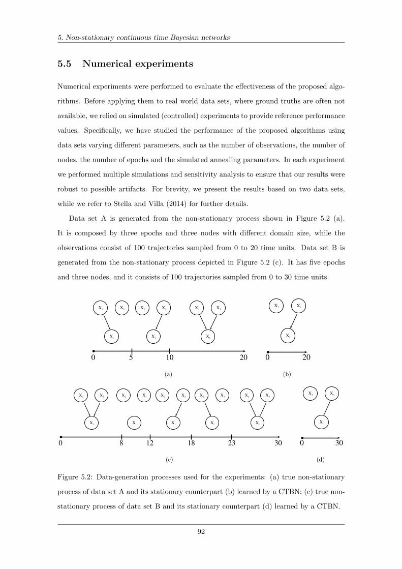
5. Non-stationary continuous time Bayesian networks
5.5 Numerical experiments
Numerical experiments were performed to evaluate the effectiveness of the proposed algo-
rithms. Before applying them to real world data sets, where ground truths are often not
available, we relied on simulated (controlled) experiments to provide reference performance
values. Specifically, we have studied the performance of the proposed algorithms using
data sets varying different parameters, such as the number of observations, the number of
nodes, the number of epochs and the simulated annealing parameters. In each experiment
we performed multiple simulations and sensitivity analysis to ensure that our results were
robust to possible artifacts. For brevity, we present the results based on two data sets,
while we refer to Stella and Villa (2014) for further details.
Data set A is generated from the non-stationary process shown in Figure 5.2 (a).
It is composed by three epochs and three nodes with different domain size, while the
observations consist of 100 trajectories sampled from 0 to 20 time units. Data set B is
generated from the non-stationary process depicted in Figure 5.2 (c). It has five epochs
and three nodes, and it consists of 100 trajectories sampled from 0 to 30 time units.
0 5 10 20
X2
X1
X3X2
X1
X3X2
X1
X3
(a)
0 20
X2
X1
X3
(b)
0 30
X2
X1
X3X2
X1
X3
128 18 23
X2
X1
X3 X2
X1
X3 X2
X1
X3
(c)
0 30
X2
X1
X3
(d)
Figure 5.2: Data-generation processes used for the experiments: (a) true non-stationary
process of data set A and its stationary counterpart (b) learned by a CTBN; (c) true non-
stationary process of data set B and its stationary counterpart (d) learned by a CTBN.
92

5. Non-stationary continuous time Bayesian networks
5.5.1 Known transition times
The first set of experiments was focused on two aspects: the ability of Algorithm 5.1 to
reconstruct the correct graphs sequence and the analysis of the impacts of the parameter
λc that regulates the creation of new edges. In the case where there are no restrictions on
the evolution of the graphs sequence, i.e. λc = 0, the optimal graphs sequence is obtained
acting greedily. Therefore, we partitioned the data sets according to the transitions times
and we applied the standard structural learning algorithm for CTBNs on each partition.
Then, the results were compared against those of Algorithm 5.1 (with λc = 0) and we
ascertained that the reconstructed graphs sequences were identical.
In the case where there are some restrictions on the evolution of the graphs sequence,
i.e. λc > 0, we analyzed the behavior of the optimal graphs sequence over time varying the
value of the parameter λc. Figure 5.3 shows the optimal graphs sequence of four nsCTBNs
reconstructed using data set A with different values of λc. In the first case (λc = 0)
the resulting graphs sequence has 3 edge changes, i.e. ∆G1 = {X2 6→ X1, X3 → X1}
and ∆G2 = {X2 → X1}. In the second case (λc = 20) we have 2 edge changes, i.e.
∆G1 = {X2 6→ X1, X3 → X1} and ∆G2 = ∅. In the third case (λc = 50) we have only one
edge change, i.e. ∆G1 = {X3 → X1} and ∆G2 = ∅. In the last case (λc = 70) the cost of
change an edge is so high that we have no changes.
0 5 10 20
X2
X1
X3X2
X1
X3X2
X1
X3
(a)
0 5 10 20
X2
X1
X3X2
X1
X3X2
X1
X3
(b)
0 5 10 20
X2
X1
X3X2
X1
X3X2
X1
X3
(c)
0 5 10 20
X2
X1
X3X2
X1
X3X2
X1
X3
(d)
Figure 5.3: Optimal graphs sequence over time for data set A varying the parameter λc:
(a) λc = 0, (b) λc = 20, (c) λc = 50 and (d) λc = 70.
93
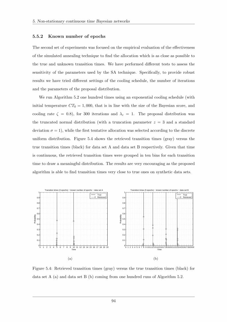
5. Non-stationary continuous time Bayesian networks
5.5.2 Known number of epochs
The second set of experiments was focused on the empirical evaluation of the effectiveness
of the simulated annealing technique to find the allocation which is as close as possible to
the true and unknown transition times. We have performed different tests to assess the
sensitivity of the parameters used by the SA technique. Specifically, to provide robust
results we have tried different settings of the cooling schedule, the number of iterations
and the parameters of the proposal distribution.
We run Algorithm 5.2 one hundred times using an exponential cooling schedule (with
initial temperature CT0 = 1, 000, that is in line with the size of the Bayesian score, and
cooling rate ζ = 0.8), for 300 iterations and λc = 1. The proposal distribution was
the truncated normal distribution (with a truncation parameter z = 3 and a standard
deviation σ = 1), while the first tentative allocation was selected according to the discrete
uniform distribution. Figure 5.4 shows the retrieved transition times (gray) versus the
true transition times (black) for data set A and data set B respectively. Given that time
is continuous, the retrieved transition times were grouped in ten bins for each transition
time to draw a meaningful distribution. The results are very encouraging as the proposed
algorithm is able to find transition times very close to true ones on synthetic data sets.
0 1 2 3 4 5 6 7 8 9 10 11 12 13 14 15 16 17 18 19 200
0.1
0.2
0.3
0.4
0.5
0.6
0.7
0.8
0.9
1
Time
Pro
babi
lity
Transition times (3 epochs) − known number of epochs − data set A
TrueRetrieved
(a)
0 1 2 3 4 5 6 7 8 9 1011121314151617181920212223242526272829300
0.1
0.2
0.3
0.4
0.5
0.6
0.7
0.8
0.9
1
Time
Pro
babi
lity
Transition times (5 epochs) − known number of epochs − data set B
TrueRetrieved
(b)
Figure 5.4: Retrieved transition times (gray) versus the true transition times (black) for
data set A (a) and data set B (b) coming from one hundred runs of Algorithm 5.2.
94
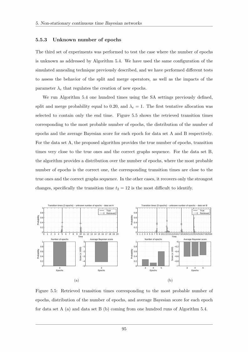
5. Non-stationary continuous time Bayesian networks
5.5.3 Unknown number of epochs
The third set of experiments was performed to test the case where the number of epochs
is unknown as addressed by Algorithm 5.4. We have used the same configuration of the
simulated annealing technique previously described, and we have performed different tests
to assess the behavior of the split and merge operators, as well as the impacts of the
parameter λe that regulates the creation of new epochs.
We run Algorithm 5.4 one hundred times using the SA settings previously defined,
split and merge probability equal to 0.20, and λe = 1. The first tentative allocation was
selected to contain only the end time. Figure 5.5 shows the retrieved transition times
corresponding to the most probable number of epochs, the distribution of the number of
epochs and the average Bayesian score for each epoch for data set A and B respectively.
For the data set A, the proposed algorithm provides the true number of epochs, transition
times very close to the true ones and the correct graphs sequence. For the data set B,
the algorithm provides a distribution over the number of epochs, where the most probable
number of epochs is the correct one, the corresponding transition times are close to the
true ones and the correct graphs sequence. In the other cases, it recovers only the strongest
changes, specifically the transition time t2 = 12 is the most difficult to identify.
0 1 2 3 4 5 6 7 8 9 10 11 12 13 14 15 16 17 18 19 200
0.2
0.4
0.6
0.8
1
Time
Pro
babi
lity
Transition times (3 epochs) − unknown number of epochs − data set A
TrueRetrieved
30
0.2
0.4
0.6
0.8
1Number of epochs
Epochs
Pro
babi
lity
3−5
−4
−3
−2
−1
0Average Bayesian score
Epochs
Sco
re (
x 10
00)
(a)
0 1 2 3 4 5 6 7 8 9 1011121314151617181920212223242526272829300
0.2
0.4
0.6
0.8
1
Time
Pro
babi
lity
Transition times (5 epochs) − unknown number of epochs − data set B
TrueRetrieved
3 4 50
0.2
0.4
0.6
0.8
1Number of epochs
Epochs
Pro
babi
lity
3 4 5−7
−6.8
−6.6
−6.4
−6.2
−6Average Bayesian score
Epochs
Sco
re (
x 10
00)
(b)
Figure 5.5: Retrieved transition times corresponding to the most probable number of
epochs, distribution of the number of epochs, and average Bayesian score for each epoch
for data set A (a) and data set B (b) coming from one hundred runs of Algorithm 5.4.
95
5. Non-stationary continuous time Bayesian networks
5.6 Discussion
After a brief introduction of the motivations of non-stationarity modeling and the state-
of-the-art methods in this context, we have presented the structural non-stationary con-
tinuous time Bayesian networks. These models allow us to represent dependencies which
change over continuous time; this aspect makes them particularly suitable to in-depth
analyze time-series data. We have provided the formal derivation of the Bayesian score
for learning these models, and we have designed and implemented three learning algo-
rithms of increasing complexity based on the available knowledge. Finally, we have tested
the proposed algorithms on synthetic data sets and illustrated their effectiveness in the
reconstruction of the correct graphs sequence.
96

Chapter 6
Markov decision processes
The probabilistic graphical models described in the previous chapters can be used within
the Markov decision process framework, which provides a model for sequential decision-
making under uncertainty. We begin by reviewing the basic concepts and algorithms,
then we move on describing factored Markov decision processes and then we conclude
the chapter discussing structured continuous time Markov decision processes with some
examples in a simplified, but meaningful trading domain.
6.1 Basic concepts
Markov decision processes have been widely used in modeling stochastic sequential decision
problems, such as many economic problems involving choices made over time and under
uncertainty, see for example Derman et al. (1975); Mendelssohn and Sobel (1980); White
(1993); Bauerle and Rieder (2011). We describe the basics of fully observable Markov
decision processes, while we refer to Bertsekas (1987); Puterman (1994); Boutilier et al.
(1999) for further material on these models.
Definition 6.1. Markov decision process (MDP), (Puterman, 1994). A MDP is defined
as a tuple (X,A, R, P ) where: X is a finite set of states; A is a finite set of actions; R
is a (bounded) reward function R : X ×A → [0, Rmax] such that R(x, a) represents the
reward obtained in state x after taking action a; and P is a Markovian transition model
such that P (x′|x, a) represents the probability of going from state x to state x′ after taking
action a.
97
6. Markov decision processes
6.1.1 Policy
A policy describes a course of action to be adopted by the decision-maker to control the
system. We are interested in Markovian, since the action choice at any state does not
depend on the system history, and stationary policies, since action choice does not depend
on the stage of the decision problem. More precisely, we define a policy as follows.
Definition 6.2. (Deterministic, stationary, Markovian) policy, (Puterman, 1994). A
policy π for an MDP is a mapping π : X → A, where π(x) is the action the decision-
maker takes in the state x.
6.1.2 Value function
An optimality criteria is used to measure the value of a policy which evaluates the rewards
accumulated by the decision-maker, as it goes through the state space executing π. The
decision-maker seeks to maximize the expected return, where the return is defined as
some specific function of the reward sequence. We focus on infinite-horizon problems
where the decision-maker is trying to maximize two types of expected returns: discounted
and average. In the discounted return case, the current value of a reward received in the
future is discounted by γ with γ ∈ [0, 1), a discount factor γ close to 0 leads to myopic
evaluation, while close to 1 leads to far-sighted evaluation. In the average return case, the
decision-maker is interested in maximizing the average reward received per time step.
Definition 6.3. Value function, (Puterman, 1994). The value function of a state x under
a policy π, denoted by V π(x), is the expected return when starting in x and following π.
The value function for the infinite-horizon discounted return is:
V π(x) = limT→∞
Eπ
[T∑t=0
γtR(X(t), π(X(t)))|X(0) = x
], (6.1)
while for the infinite-horizon average return ρπ, the value function is:
V π(x) = limT→∞
1
TEπ
[T∑t=0
R(X(t), π(X(t)))
]= ρπ, (6.2)
where X(t) is a random variable representing the state of the system after t steps. In
equation (6.2) we assume that for any policy π, the resulting Markov chain P (x′|x, π(x))
is ergodic, and hence the average return ρπ is unique, independent of the starting state
(Puterman, 1994).
98
6. Markov decision processes
6.1.3 Bellman operators
Value functions allow us to define a partial ordering over policies: a policy π is better than
or equal to another policy π′ if its expected return is greater than or equal to that of π′
for all states, i.e. π ≥ π′ if and only if V π(x) ≥ V π′(x) for all x ∈ X. There is at least
one optimal policy π∗ that is better than or equal to all other policies; its value function
is the optimal value function V ∗ and is defined as:
V ∗(x) = maxπ{V π(x)}, ∀x ∈X. (6.3)
The optimal value function and the optimal policy are related to the Bellman (1957)
operators. The Bellman operators allow us to express relationships between the value of
a state and the values of its successor states: the value of the start state x is equal to the
immediate reward plus the (discounted) value of the successor state x′.
Definition 6.4. Bellman operator, (Bellman, 1957). The Bellman operator, denoted as
Fπ : R|X| → R|X|, for a policy π is defined as follows:
(FπV )(x) = R(x, π(x)) + γ∑x′
P (x′|x, π(x))V (x′). (6.4)
The value function of a policy π is the fixed point of Fπ such that V π = FπV π.
As reported in equation (6.3), the optimal value function is defined by a set of non-
linear equations; thus, the value of a state must be the maximal expected value achievable
by any policy starting at that state.
Definition 6.5. Bellman optimality operator, (Bellman, 1957). The Bellman optimality
operator, denoted as F∗ : R|X| → R|X|, is defined as:
(F∗V )(x) = maxa
{R(x, a) + γ
∑x′
P (x′|x, a)V (x′)
}. (6.5)
The optimal value function V ∗ is the fixed point of F∗ such that V ∗ = F∗V ∗.
We can define the policy obtained by acting greedily relative to V as follows:
greedy(V )(x) = arg maxa
{R(x, a) + γ
∑x′
P (x′|x, a)V (x′)
}. (6.6)
The greedy policy relative to the optimal value function V ∗ is the optimal policy π∗ =
greedy(V ∗).
99
6. Markov decision processes
6.2 Solving Markov decision processes
Solving a Markov decision process consists of constructing an optimal policy π∗. There are
different algorithms to compute optimal policies in MDPs; we present two most popular
dynamic programming methods, namely policy iteration and value iteration, and then we
introduce the linear programming method.
6.2.1 Policy iteration
The policy iteration algorithm iterates over policies, producing an improved policy at
each iteration. This algorithm consists of two components, called policy evaluation and
policy improvement, and it can be shown to converge to the optimal policy (Howard, 1960;
Bertsekas and Tsitsiklis, 1996). This algorithm can be described as follows.
For the policy evaluation part (lines 3 - 10 of Algorithm 6.1), consider a sequence of
value functions V0, V1, . . . , each mapping X to R. The initial value function, V0, is chosen
arbitrarily, and the successive value functions are obtained by using the Bellman operator
(6.4) as an update rule for each state x ∈ X. The sequence (Vj)∞j=0 converges to V π
because of the Bellman operator; thus, V∞ = V π is a fixed point for this update rule. In
practice, it is possible to stop the policy evaluation part when the Bellman error of Vj is less
then a small amount ε > 0, i.e. err(Vj) = ||F∗Vj − Vj ||∞ = maxx{F∗Vj(x)− Vj(x)} < ε.
To produce successive approximation Vj+1 from Vj , the iterative policy evaluation updates
the value of one state based on the values of all possible successor states (rather than on
a sample of the next state), so it performs a so called full backup.
Once we have determined the value function V π for an arbitrary policy π, we can
perform the policy improvement procedure (lines 12 - 18 of Algorithm 6.1) by selecting
the greedy policy for each state x according to equation (6.6).
Each policy evaluation part is started with the value function from the previous policy.
This typically results in a great increase of the speed of convergence of policy evaluation,
so the algorithm converges in a few iterations, but in O(|X|2×|A|+ |X|3) (Littman et al.,
1995). Mansour and Singh (1999) gave an upper bound on the number of iterations equal
to |A||X|/|X|, while Ye (2011) proved that policy iteration is a strongly polynomial-time
algorithm for solving MDPs with a fixed discount factor.
100

6. Markov decision processes
6.2.2 Value iteration
Value iteration (Bellman, 1957) can be seen as a special case of the policy iteration when
the policy evaluation step is stopped after just one sweep (i.e. one backup of each state).
Thus, the value iteration algorithm effectively combines in each of its sweeps one sweep
of policy evaluation and one sweep of policy improvement (lines 4 - 8 of Algorithm 6.2).
Unlike policy iteration, there is no explicit policy, so the intermediate value functions may
not correspond to any policy. Like policy iteration, value iteration requires an infinite
number of iterations to converge to V ∗. In practice, it is possible to stop the algorithm
once the value function changes by only a small amount ε > 0 in a sweep (Sutton and Barto,
1998). Value iteration approximates the optimal value function by successive iterations
that can be performed in O(|X|2 × |A|), but the number of iterations required can grow
exponentially in the discount factor (Condon, 1992).
Algorithm 6.1 Policy iteration
Require: MDP (X,A, R, P ), ε > 0.
Ensure: optimal policy π∗.
1: Initialize V (x), π(x) ∀x ∈X2: repeat
3: repeat
4: ∆← 0
5: for each x ∈X do
6: v ← V (x)
7: V (x)← (FπV )(x)
8: ∆← max{∆, |v − V (x)|}9: end for
10: until (∆ < ε)
11: stableπ ← true
12: for each x ∈X do
13: a← π(x)
14: π(x)← greedy(V )(x)
15: if (a 6= π(x)) then
16: stableπ ← false
17: end if
18: end for
19: until (stableπ)
Algorithm 6.2 Value iteration
Require: MDP (X,A, R, P ), ε > 0.
Ensure: optimal policy π∗.
1: Initialize V (x) ∀x ∈X2: repeat
3: ∆← 0
4: for each x ∈X do
5: v ← V (x)
6: V (x)← (F∗V )(x)
7: ∆← max{∆, |v − V (x)|}8: end for
9: until (∆ < ε)
10: for each x ∈X do
11: π(x)← greedy(V )(x)
12: end for
101
6. Markov decision processes
6.2.3 Linear programming
Linear programming provides an alternative method compared to value iteration and pol-
icy iteration for solving MDPs, where the problem of finding a value function is formulated
as a linear program (LP), see D’Epenoux (1963). Let S be the number of possible states
of system, then the LP variables are V1, . . . , VS , where each Vs represents V (xs), i.e. the
value of starting at the s-th state of the system. The linear program is defined as follows:
vars : V1, . . . , VS (6.7)
min :S∑s=1
α(xs)Vs (6.8)
s.t. : Vs ≥ R(xs, a) + γ∑j
P (xj |xs, a)V (xj), ∀xs ∈X,∀a ∈ A, (6.9)
where α(xs) are positive state relevance weights. Note that the policy is implicitly repre-
sented by the slack variables of the LP. In fact, for each xs there is at least one action a
for which the corresponding state value constraint is tight, i.e. the optimal action for xs.
There are several algorithms for solving LPs (Vanderbei, 2001), among which the well
known simplex algorithm introduced by Dantzig (1963). This algorithm starts at a vertex
of the polyhedron corresponding to the LP and then follows edges of the polyhedron that
lead to vertices of lower value, until an optimal vertex is reached, or an edge along which
the objective function is unbounded from below is found. The choice of which edge to
follow is controlled by a pivoting rule; for example, the Dantzig’s pivoting rule asserts that
the non-basic variable with the most negative reduced cost is chosen to enter the basis.
There is a close connection between policy iteration method, which updates actions
in multiple states simultaneously, and the simplex algorithm, which updates an action in
only one state at a time. In fact, a violated constraint in the LP formulation provides an
opportunity for policy improvement by pivoting on the corresponding variable in a simplex
algorithm for the dual problem (Ye, 2011).
The simplex method is very efficient in practice and, even if its worst-case complexity
is exponential (Klee and Minty, 1972), it has been proved to be strongly polynomial when
used to solve MDPs with any value of the discount factor (Post and Ye, 2013).
102
6. Markov decision processes
6.3 Factored Markov decision processes
One of the main problems with MDPs is that the number of possible states becomes
very large when they are used to model real life domains. In fact, these domains can
have a significant internal structure that MDPs are not able to model. We refer to two
main types of structure: additive, i.e. large scale systems can often be decomposed into
a combination of locally interacting components, and context-specific, i.e. large systems
may be influenced directly by only a small number of parts at any given point in time.
Factored MDPs are one approach to represent large and structured domains effectively
(Boutilier et al., 1995). In this framework, a state is described implicitly as an assignment
of values to some set of state variables and a dynamic Bayesian network is then used as a
compact representation of the transition dynamics.
Definition 6.6. Factored MDP, (Boutilier et al., 1995). A factored MDP is an MDP
(X,A, R, P ) where: the set of states X is described via a set of random variables X =
{X1, . . . , XN}; A is the finite set of actions; R is the reward function and it is factored
additively into a set of L localized functions: R(x, a) =∑L
l=1Rl(Lal , a) ∈ R in which the
Scope[Rl] is restricted to Lal ⊆ X; the transition model P is a set of dynamic Bayesian
networks, one network Ba2 for each action a ∈ A. The transition graph of a DBN is a
two-layer directed acyclic graph GBa2T whose nodes are {X1, . . . , XN , X′1, . . . , X
′N}. Each
node X ′ is associated with a conditional probability distribution PBa2T (X ′|Pa(X ′)). The
transition probability is then defined as P (x′|x, a) =∏X′ PBa2T (X ′ = x′n|Pa(X ′) = pau).
Factorization allows a very large MDP to be represented compactly; however, solving
it exactly may still be intractable: exact solution algorithms require the manipulation of
the value function, whose representation is linear in the number of states, but exponential
in the number of state variables. Moreover, factored dynamics and rewards do not ensure
that the value function has a factored representation (Koller and Parr, 1999). Dynamic
programming methods have been adapted to factored representations, such as structured
policy iteration (Boutilier et al., 1995) and structured value iteration (Boutilier et al.,
2000), that exploit the context-specific structure in the value function using decision trees
manipulations. Approximate linear programming methods have emerged as promising
approaches to solve them efficiently (Guestrin et al., 2003).
103

6. Markov decision processes
6.3.1 Approximate linear programming
A key to performing efficient computations over the exponentially-sized state spaces en-
countered in factored MDPs is the use of an approximate value function. A very popular
choice for this approximation is by using linear regression (Bellman and Dreyfus, 1959;
Tsitsiklis and van Roy, 1996; Koller and Parr, 1999), where the space of allowable value
functions is specified via a set of basis functions.
Definition 6.7. Factored linear value function, (Koller and Parr, 1999). A factored linear
value function over a set of basis functions H = {h1, . . . , hK} is a function V that can be
written as V (x) =∑K
k=1wkhk(x) for some coefficients w = (w1, . . . , wK)′.
Once the set of basis functions H has been selected, the problem becomes one of
finding values for the weights w such that Hw will yield a good approximation to the
true value function. One efficient approach to solving this problem is based on the LP
formulation defined in (6.7)-(6.9). Specifically, Schweitzer and Seidmann (1985) restricted
the space of allowable value functions to the linear space spanned by K basis functions.
The approximate linear program (ALP) formulation for factored MDPs is:
vars : w1, . . . , wK (6.10)
min :∑x
α(x)K∑k=1
wkhk(x) (6.11)
s.t. :
K∑k=1
wkhk(x) ≥ R(x, a) + γ∑x′
P (x′|x, a)
K∑k=1
wkhk(x′), ∀x ∈X, ∀a ∈ A. (6.12)
This ALP is guaranteed to be feasible if a constant function, i.e. a function with
the same constant value for all states, is included in the set of basis function (Guestrin
et al., 2002). We have to point out two aspects of this ALP formulation. Firstly, the
choice of state relevance weights α(x) becomes important because, unlike the exact case,
the solution obtained may differ for different choices of the positive weights. Secondly,
in general, there is no guarantee about the quality of the greedy policy generated from
the approximation Hw. However, de Farias and van Roy (2003) provided an analysis of
the error relative to that of the best possible approximation in the subspace and some
guidance about the selection of α(x) in order to improve the quality of the approximation.
104

6. Markov decision processes
6.3.2 Backprojection function
A key component of the ALP formulation is the computation of the one-step lookahead
function, called backprojection, gak(x) of the basis function hk for the action a:
gak(x) =∑x′
P (x′|x, a)hk(x′). (6.13)
This computation is performed efficiently when the transition model is factored using
a DBN, and each basis functions hk has scope restricted to a small set of variables, i.e.
Scope[hk] = Ck. In fact, the scope of the backprojection gak through a DBN Ba2 is the set of
parents of C ′k in the transition graph GBa2T , i.e. the Scope[gak ] =⋃X′n∈C′k
PaBa2T (X ′n) = Bak
(Guestrin et al., 2003). The advantage is that each backprojection can be computed by
only enumerating settings of variables in Bak, rather than settings of all variables X. The
cost of the computation depends linearly on |V al(Bak)|, which depends on Ck, and on the
complexity of the process dynamics. The backprojection of the basis function hk is then
computed as follows:
gak(x) =∑c′∈C′k
∏X′n∈C′k
PBa2 (c′[X ′n]|bak, a)hk(c′), ∀bak ∈ Ba
k, (6.14)
where c′[X ′n] denotes the value of variable X ′n in the instantiation c′.
6.3.3 Efficient constraints representation
The ALP formulation has the effect of reducing the number of free variables in the linear
program from |X| to K, but the number of constraints remains |X|× |A|. However, given
that the functionals in the constraints (6.12) have restricted scope, i.e. the constraints can
be satisfied in a structured form and without being enumerated exhaustively, it is possible
to use some methods to exploit this peculiarity.
Guestrin et al. (2003) observed that the constraints (6.12) are all in the form:
0 ≥ R(x, a) +K∑k=1
wkFk(x, a), ∀x ∈X, ∀a ∈ A, (6.15)
where Fk(x, a) = γgak(x)−hk(x) has the scope restricted to Ck ∪Bak. Thus, it is possible
to replace the entire set of constraints (6.15) by |A| equivalent non-linear constraints:
0 ≥ maxx
{R(x, a) +
K∑k=1
wkFk(x, a)
}, ∀a ∈ A. (6.16)
105

6. Markov decision processes
The approximate linear program formulation reported in (6.10)-(6.12) becomes:
vars : w1, . . . , wK (6.17)
min :
K∑k=1
αkwk (6.18)
s.t. : 0 ≥ maxx
{R(x, a) +
K∑k=1
wk (γgak(x)− hk(x))
}, ∀a ∈ A. (6.19)
The basis weights αk are defined as αk =∑ck∈Ck α(ck)hk(ck), where α(ck) represents the
marginal of the state relevance weights over V al(Ck) of the basis function hk.
The new set of non-linear constraints (6.19) can be implemented by a set of linear
constraints using a construction that follows the structure of the variable elimination
algorithm in BNs (Guestrin et al., 2003). The main idea is maximizing over variables one
at a time instead of summing all functions and then doing the maximization. Note that
computing the optimal elimination order is an NP-hard problem (Arnborg et al., 1987);
however, good heuristics have been introduced (Reed, 1992; Becker and Geiger, 2001).
Schuurmans and Patrascu (2001) solved the constraints satisfaction problem by the
cutting plane method (Bertsekas and Tsitsiklis, 1996). The approach iteratively searches
for the most violated constraint for each action a:
arg maxx
{R(x, a) +
K∑k=1
w(i)k Fk(x, a)
}, (6.20)
with respect to the solution w(i) of a relaxed ALP in the i-th iteration. The most violated
constraint is added to the ALP, which is then solved for a new vector w(i+1). This
procedure is iterated until no violated constraint is found; the last vector w(i) is then an
optimal solution to the ALP problem.
The space complexity of both methods is exponential in the tree-width of the con-
straints space. However, such problems can be still solved approximately. For example,
de Farias and van Roy (2004) proposed Monte Carlo approximations of the constraints
space. Kveton and Hauskrecht (2005) introduced a Markov chain Monte Carlo sample
for searching the most violated constraints. Kveton and Hauskrecht (2008) described a
different ALP based on the inner approximations to the feasible region; in particular,
they decomposed the constraints space into a set of low dimensional spaces without an
exponential dependence on the tree-width of the original constraints space.
106
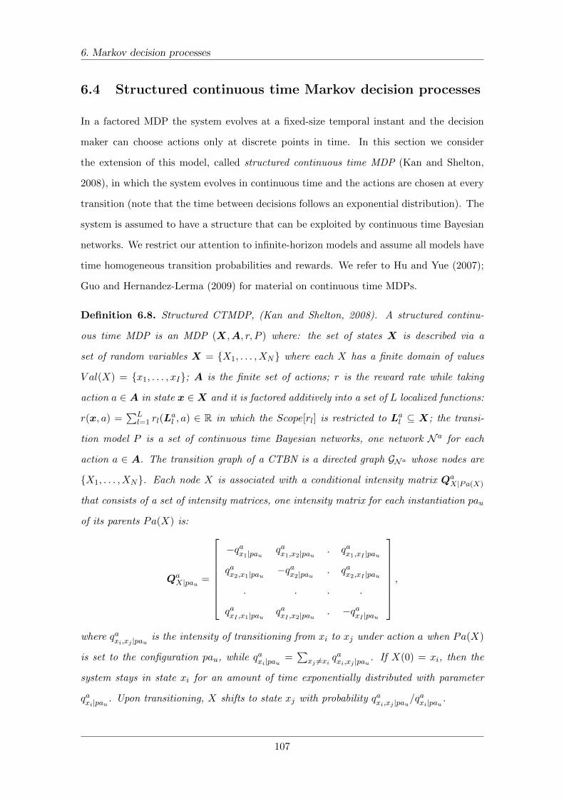
6. Markov decision processes
6.4 Structured continuous time Markov decision processes
In a factored MDP the system evolves at a fixed-size temporal instant and the decision
maker can choose actions only at discrete points in time. In this section we consider
the extension of this model, called structured continuous time MDP (Kan and Shelton,
2008), in which the system evolves in continuous time and the actions are chosen at every
transition (note that the time between decisions follows an exponential distribution). The
system is assumed to have a structure that can be exploited by continuous time Bayesian
networks. We restrict our attention to infinite-horizon models and assume all models have
time homogeneous transition probabilities and rewards. We refer to Hu and Yue (2007);
Guo and Hernandez-Lerma (2009) for material on continuous time MDPs.
Definition 6.8. Structured CTMDP, (Kan and Shelton, 2008). A structured continu-
ous time MDP is an MDP (X,A, r, P ) where: the set of states X is described via a
set of random variables X = {X1, . . . , XN} where each X has a finite domain of values
V al(X) = {x1, . . . , xI}; A is the finite set of actions; r is the reward rate while taking
action a ∈ A in state x ∈X and it is factored additively into a set of L localized functions:
r(x, a) =∑L
l=1 rl(Lal , a) ∈ R in which the Scope[rl] is restricted to Lal ⊆ X; the transi-
tion model P is a set of continuous time Bayesian networks, one network N a for each
action a ∈ A. The transition graph of a CTBN is a directed graph GNa whose nodes are
{X1, . . . , XN}. Each node X is associated with a conditional intensity matrix QaX|Pa(X)
that consists of a set of intensity matrices, one intensity matrix for each instantiation pau
of its parents Pa(X) is:
QaX|pau =
−qax1|pau qax1,x2|pau . qax1,xI |pau
qax2,x1|pau −qax2|pau . qax2,xI |pau
. . . .
qaxI ,x1|pau qaxI ,x2|pau . −qaxI |pau
,
where qaxi,xj |pau is the intensity of transitioning from xi to xj under action a when Pa(X)
is set to the configuration pau, while qaxi|pau =∑
xj 6=xi qaxi,xj |pau. If X(0) = xi, then the
system stays in state xi for an amount of time exponentially distributed with parameter
qaxi|pau. Upon transitioning, X shifts to state xj with probability qaxi,xj |pau/qaxi|pau.
107
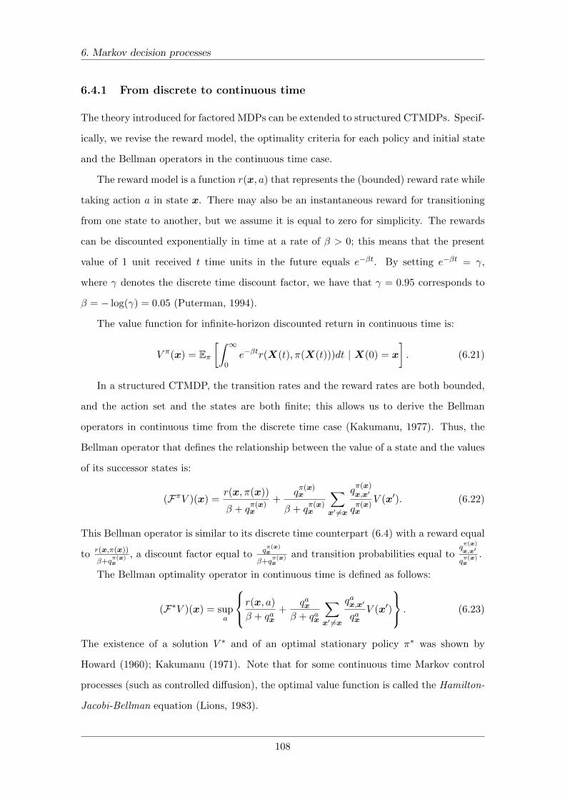
6. Markov decision processes
6.4.1 From discrete to continuous time
The theory introduced for factored MDPs can be extended to structured CTMDPs. Specif-
ically, we revise the reward model, the optimality criteria for each policy and initial state
and the Bellman operators in the continuous time case.
The reward model is a function r(x, a) that represents the (bounded) reward rate while
taking action a in state x. There may also be an instantaneous reward for transitioning
from one state to another, but we assume it is equal to zero for simplicity. The rewards
can be discounted exponentially in time at a rate of β > 0; this means that the present
value of 1 unit received t time units in the future equals e−βt. By setting e−βt = γ,
where γ denotes the discrete time discount factor, we have that γ = 0.95 corresponds to
β = − log(γ) = 0.05 (Puterman, 1994).
The value function for infinite-horizon discounted return in continuous time is:
V π(x) = Eπ[∫ ∞
0e−βtr(X(t), π(X(t)))dt | X(0) = x
]. (6.21)
In a structured CTMDP, the transition rates and the reward rates are both bounded,
and the action set and the states are both finite; this allows us to derive the Bellman
operators in continuous time from the discrete time case (Kakumanu, 1977). Thus, the
Bellman operator that defines the relationship between the value of a state and the values
of its successor states is:
(FπV )(x) =r(x, π(x))
β + qπ(x)x
+qπ(x)x
β + qπ(x)x
∑x′ 6=x
qπ(x)x,x′
qπ(x)x
V (x′). (6.22)
This Bellman operator is similar to its discrete time counterpart (6.4) with a reward equal
to r(x,π(x))
β+qπ(x)x
, a discount factor equal to qπ(x)x
β+qπ(x)x
and transition probabilities equal toqπ(x)
x,x′
qπ(x)x
.
The Bellman optimality operator in continuous time is defined as follows:
(F∗V )(x) = supa
r(x, a)
β + qax+
qaxβ + qax
∑x′ 6=x
qax,x′
qaxV (x′)
. (6.23)
The existence of a solution V ∗ and of an optimal stationary policy π∗ was shown by
Howard (1960); Kakumanu (1971). Note that for some continuous time Markov control
processes (such as controlled diffusion), the optimal value function is called the Hamilton-
Jacobi-Bellman equation (Lions, 1983).
108
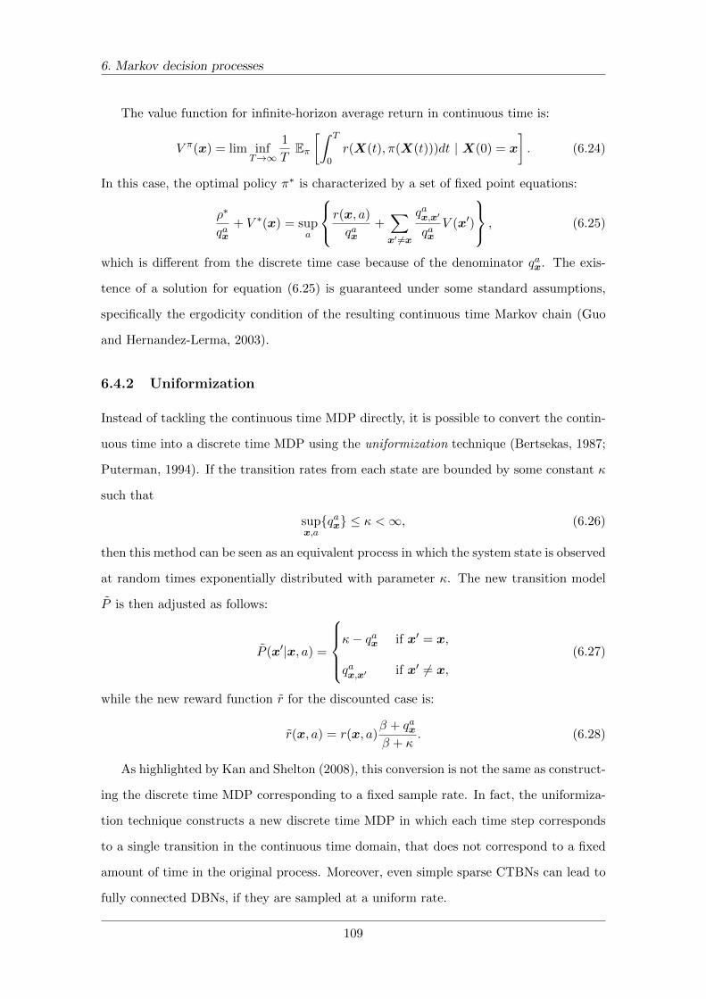
6. Markov decision processes
The value function for infinite-horizon average return in continuous time is:
V π(x) = lim infT→∞
1
TEπ[∫ T
0r(X(t), π(X(t)))dt | X(0) = x
]. (6.24)
In this case, the optimal policy π∗ is characterized by a set of fixed point equations:
ρ∗
qax+ V ∗(x) = sup
a
r(x, a)
qax+∑x′ 6=x
qax,x′
qaxV (x′)
, (6.25)
which is different from the discrete time case because of the denominator qax. The exis-
tence of a solution for equation (6.25) is guaranteed under some standard assumptions,
specifically the ergodicity condition of the resulting continuous time Markov chain (Guo
and Hernandez-Lerma, 2003).
6.4.2 Uniformization
Instead of tackling the continuous time MDP directly, it is possible to convert the contin-
uous time into a discrete time MDP using the uniformization technique (Bertsekas, 1987;
Puterman, 1994). If the transition rates from each state are bounded by some constant κ
such that
supx,a{qax} ≤ κ <∞, (6.26)
then this method can be seen as an equivalent process in which the system state is observed
at random times exponentially distributed with parameter κ. The new transition model
P is then adjusted as follows:
P (x′|x, a) =
κ− qax if x′ = x,
qax,x′ if x′ 6= x,
(6.27)
while the new reward function r for the discounted case is:
r(x, a) = r(x, a)β + qaxβ + κ
. (6.28)
As highlighted by Kan and Shelton (2008), this conversion is not the same as construct-
ing the discrete time MDP corresponding to a fixed sample rate. In fact, the uniformiza-
tion technique constructs a new discrete time MDP in which each time step corresponds
to a single transition in the continuous time domain, that does not correspond to a fixed
amount of time in the original process. Moreover, even simple sparse CTBNs can lead to
fully connected DBNs, if they are sampled at a uniform rate.
109
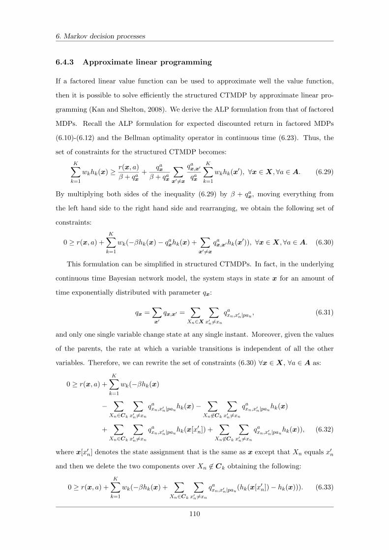
6. Markov decision processes
6.4.3 Approximate linear programming
If a factored linear value function can be used to approximate well the value function,
then it is possible to solve efficiently the structured CTMDP by approximate linear pro-
gramming (Kan and Shelton, 2008). We derive the ALP formulation from that of factored
MDPs. Recall the ALP formulation for expected discounted return in factored MDPs
(6.10)-(6.12) and the Bellman optimality operator in continuous time (6.23). Thus, the
set of constraints for the structured CTMDP becomes:
K∑k=1
wkhk(x) ≥ r(x, a)
β + qax+
qaxβ + qax
∑x′ 6=x
qax,x′
qax
K∑k=1
wkhk(x′), ∀x ∈X, ∀a ∈ A. (6.29)
By multiplying both sides of the inequality (6.29) by β + qax, moving everything from
the left hand side to the right hand side and rearranging, we obtain the following set of
constraints:
0 ≥ r(x, a) +K∑k=1
wk(−βhk(x)− qaxhk(x) +∑x′ 6=x
qax,x′hk(x′)), ∀x ∈X, ∀a ∈ A. (6.30)
This formulation can be simplified in structured CTMDPs. In fact, in the underlying
continuous time Bayesian network model, the system stays in state x for an amount of
time exponentially distributed with parameter qx:
qx =∑x′
qx,x′ =∑Xn∈X
∑x′n 6=xn
qaxn,x′n|pau , (6.31)
and only one single variable change state at any single instant. Moreover, given the values
of the parents, the rate at which a variable transitions is independent of all the other
variables. Therefore, we can rewrite the set of constraints (6.30) ∀x ∈X, ∀a ∈ A as:
0 ≥ r(x, a) +K∑k=1
wk(−βhk(x)
−∑
Xn∈Ck
∑x′n 6=xn
qaxn,x′n|pauhk(x)−∑
Xn 6∈Ck
∑x′n 6=xn
qaxn,x′n|pauhk(x)
+∑
Xn∈Ck
∑x′n 6=xn
qaxn,x′n|pauhk(x[x′n]) +∑
Xn 6∈Ck
∑x′n 6=xn
qaxn,x′n|pauhk(x)), (6.32)
where x[x′n] denotes the state assignment that is the same as x except that Xn equals x′n
and then we delete the two components over Xn 6∈ Ck obtaining the following:
0 ≥ r(x, a) +
K∑k=1
wk(−βhk(x) +∑
Xn∈Ck
∑x′n 6=xn
qaxn,x′n|pau(hk(x[x′n])− hk(x))). (6.33)
110
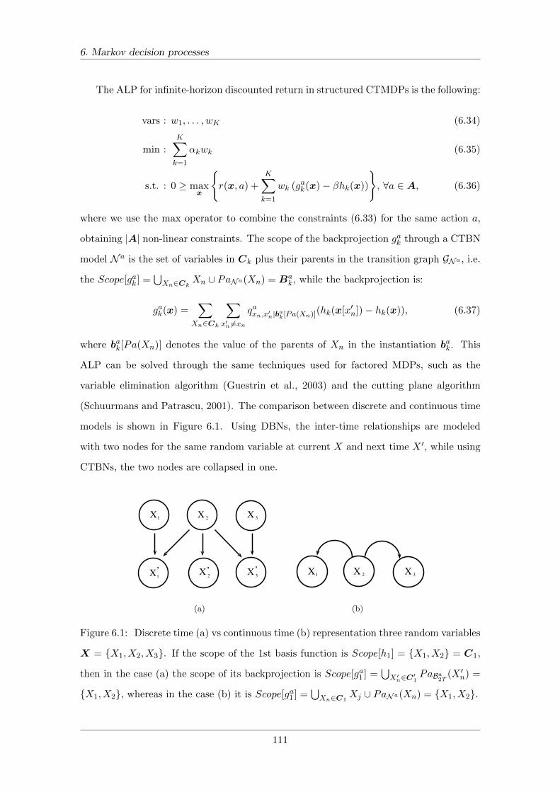
6. Markov decision processes
The ALP for infinite-horizon discounted return in structured CTMDPs is the following:
vars : w1, . . . , wK (6.34)
min :
K∑k=1
αkwk (6.35)
s.t. : 0 ≥ maxx
{r(x, a) +
K∑k=1
wk (gak(x)− βhk(x))
}, ∀a ∈ A, (6.36)
where we use the max operator to combine the constraints (6.33) for the same action a,
obtaining |A| non-linear constraints. The scope of the backprojection gak through a CTBN
model N a is the set of variables in Ck plus their parents in the transition graph GNa , i.e.
the Scope[gak ] =⋃Xn∈Ck Xn ∪ PaNa(Xn) = Ba
k, while the backprojection is:
gak(x) =∑
Xn∈Ck
∑x′n 6=xn
qaxn,x′n|bak[Pa(Xn)](hk(x[x′n])− hk(x)), (6.37)
where bak[Pa(Xn)] denotes the value of the parents of Xn in the instantiation bak. This
ALP can be solved through the same techniques used for factored MDPs, such as the
variable elimination algorithm (Guestrin et al., 2003) and the cutting plane algorithm
(Schuurmans and Patrascu, 2001). The comparison between discrete and continuous time
models is shown in Figure 6.1. Using DBNs, the inter-time relationships are modeled
with two nodes for the same random variable at current X and next time X ′, while using
CTBNs, the two nodes are collapsed in one.
X1 X 2 X 3
X1X 2 X 3
’ ’ ’
(a)
X1 X 2 X 3
(b)
Figure 6.1: Discrete time (a) vs continuous time (b) representation three random variables
X = {X1, X2, X3}. If the scope of the 1st basis function is Scope[h1] = {X1, X2} = C1,
then in the case (a) the scope of its backprojection is Scope[ga1 ] =⋃X′n∈C′1
PaBa2T (X ′n) =
{X1, X2}, whereas in the case (b) it is Scope[ga1 ] =⋃Xn∈C1
Xj ∪ PaNa(Xn) = {X1, X2}.
111
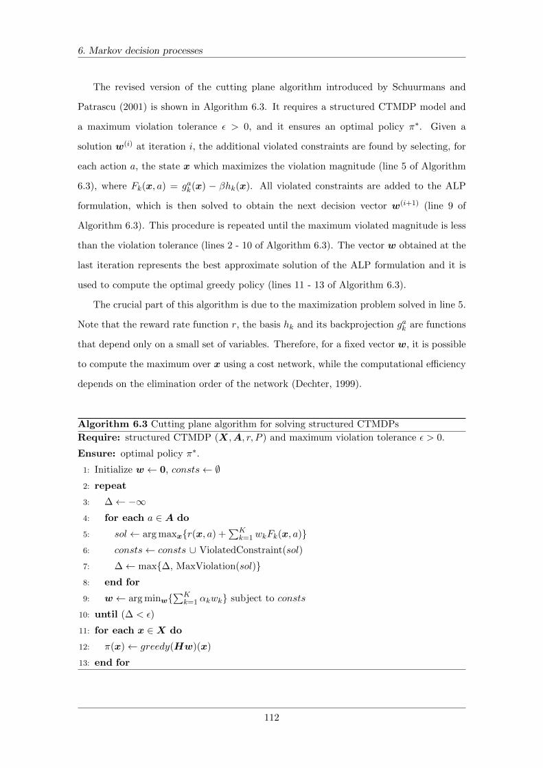
6. Markov decision processes
The revised version of the cutting plane algorithm introduced by Schuurmans and
Patrascu (2001) is shown in Algorithm 6.3. It requires a structured CTMDP model and
a maximum violation tolerance ε > 0, and it ensures an optimal policy π∗. Given a
solution w(i) at iteration i, the additional violated constraints are found by selecting, for
each action a, the state x which maximizes the violation magnitude (line 5 of Algorithm
6.3), where Fk(x, a) = gak(x) − βhk(x). All violated constraints are added to the ALP
formulation, which is then solved to obtain the next decision vector w(i+1) (line 9 of
Algorithm 6.3). This procedure is repeated until the maximum violated magnitude is less
than the violation tolerance (lines 2 - 10 of Algorithm 6.3). The vector w obtained at the
last iteration represents the best approximate solution of the ALP formulation and it is
used to compute the optimal greedy policy (lines 11 - 13 of Algorithm 6.3).
The crucial part of this algorithm is due to the maximization problem solved in line 5.
Note that the reward rate function r, the basis hk and its backprojection gak are functions
that depend only on a small set of variables. Therefore, for a fixed vector w, it is possible
to compute the maximum over x using a cost network, while the computational efficiency
depends on the elimination order of the network (Dechter, 1999).
Algorithm 6.3 Cutting plane algorithm for solving structured CTMDPs
Require: structured CTMDP (X,A, r, P ) and maximum violation tolerance ε > 0.
Ensure: optimal policy π∗.
1: Initialize w ← 0, consts← ∅2: repeat
3: ∆← −∞4: for each a ∈ A do
5: sol← arg maxx{r(x, a) +∑K
k=1wkFk(x, a)}6: consts← consts ∪ ViolatedConstraint(sol)
7: ∆← max{∆, MaxViolation(sol)}8: end for
9: w ← arg minw{∑K
k=1 αkwk} subject to consts
10: until (∆ < ε)
11: for each x ∈X do
12: π(x)← greedy(Hw)(x)
13: end for
112
6. Markov decision processes
6.5 Trading in structured continuous time domains
We consider the continuous time version of a simplified trading domain in which a portfolio
manager has to construct a portfolio choosing among N securities. These securities can
rise or fall randomly, and at any point in time the portfolio manager has to choose to buy,
sell or be neutral about one of them in order to maximize the expected discounted return.
In this context, it is possible to exploit both the additive feature of the domain, as it can
be decomposed into individual securities, and the context-specific feature, as we consider
that each security is influenced directly by only a small number of other securities that
we call neighbors. Note that a similar problem has been presented by Strehl et al. (2007)
where they used a factored MDP to model a simple stock trading domain.
6.5.1 Market dynamics
The continuous time domain is composed of a set of N securities Y and a set of N security-
owner variables Z; so the total state variables are X = Y ∪Z with N × 2 variables. Each
security Yn is modeled as a binary random variable, Yn = 1 means that the security is
rising, while Yn = 0 is falling. The security-owner variable Zn is also binary, if the portfolio
manager holds the n-th security, then Zn = 1, otherwise Zn = 0.
The market dynamics implement the basic idea that a falling security induces its
neighbors to fall more quickly: the amount of time a securities Yn is rising until it falls
follows an exponential distribution with parameter q1 = qid1 + qsys1 × number of falling
neighbors / total neighbors, while the amount of time a securities Yn is falling until it rises
follows an exponential distribution with parameter: q0 = qid0 + qsys0 × number of rising
neighbors / total neighbors. Both q1 and q0 are composed of an idiosyncratic part, qid,
specific of each security plus a systematic part, qsys, that depends on the local market
conditions. Note that the idea of distinguishing between idiosyncratic and systematic
components is widely accepted in finance (Elton et al., 2010).
At any point in time the portfolio manager must choose to buy (Bn) or sell (Sn) a
security Yn, or do nothing (Nothing), so we have A = {B1, S1, . . . BN , SN , Nothing} with
|A| = (N × 2) + 1. The security-owner variables Z are used to control the exposures, i.e.
it is not possible to buy a security already owned, or sell a security not owned.
113

6. Markov decision processes
The portfolio manager receives a global reward rate defined as the sum of N local
reward rate functions, one for each security, such that r(x, a) =∑N
l=1 rl(Yl, Zl, a) ∈ R
with Scope[rl] restricted to {Yl, Zl} ⊆X. The portfolio manager receives a reward based
on the ownership of rising and falling securities according to the following definition:
rl(Yl, Zl) =
2.0 if Yl = 1 and Zl = 1,
1.5 if Yl = 0 and Zl = 0,
0.5 if Yl = 1 and Zl = 0,
0.0 if Yl = 0 and Zl = 1.
(6.38)
6.5.2 Proposed solution
A structured CTMDP can be used to model this dynamic context and it can be solved
by the ALP (6.34)-(6.36) formulation. In order to apply this ALP we have to specify four
elements: a CTBN model for each action, the basis functions, the backprojections of the
basis functions and the basis weights.
For each action, we construct a CTBN model where the securities Y are identified as
nodes. These nodes are connected according to a given structure that models the behavior
of the interactions among securities. The entries of the conditional intensity matrices can
be the same for all securities or be different as specified in the market dynamics section.
We use K = N basis functions with Scope[hk] = {Yk} = Ck to approximate the value
function. Each basis function hk is defined as follows:
hk(Yk) =
1.0 if Yk = 1,
0.0 if Yk = 0.
(6.39)
The scope of the backprojection gak is {Yk} ∪ {Yn|Yn ∈ neighbors(Yk)} = Bak, while
the backprojection of the k-th basis function hk is defined as follows:
gak(x) = qayk,y′k|bak[neighbors(Yk)](hk(x[y′k])− hk(x)). (6.40)
For the basis weight αk =∑ck∈Ck α(ck)hk(ck), we use uniform state relevance weights,
so α(ck) = 1|Ck| = 1
2 . Finally, it is possible to solve the ALP problem using the same
techniques used for factored MDPs, such as the variable elimination algorithm and the
cutting plane algorithm defined in the previous sections.
114

6. Markov decision processes
6.5.3 Examples with different structures
We consider two examples with different structures using the solution previously described.
In the first scenario, we assume to have only two securities, Y1 and Y2, so the set of
states is X = {Y1, Y2, Z1, Z2} and the set of actions is A = {B1, S1, B2, S2, Nothing}. We
use two basis functions: h1 with Scope[h1] = {Y1} and h2 with Scope[h2] = {Y2} both
defined as in (6.39). The CTBN model depicted in Figure 6.2 (a) is used to represent the
interactions among the two securities and this structure is maintained for all actions. For
the security Y1, we assume that qid1 = 1.0, qsys1 = 2.0, and qid0 = 0.5, qsys0 = 2.0, so its
intensity matrices are defined as follows:
QY1|Y2=0 =
−0.5 0.5
3.0 −3.0
, QY1|Y2=1 =
−2.5 2.5
1.0 −1.0
. (6.41)
For security Y2, we assume that qid1 = 1.2, qsys1 = 1.8, and qid0 = 0.7, qsys0 = 1.8, so its
intensity matrices are the following:
QY2|Y1=0 =
−0.7 0.7
3.0 −3.0
, QY2|Y1=1 =
−2.5 2.5
1.2 −1.2
. (6.42)
The backprojections defined in (6.40) are used to set and solve the ALP (6.34)-(6.36).
The optimal policy extracted from its solution is shown in Figure 6.2 (b) in which for each
possible state, grouped by {Y1, Z1} and {Y2, Z2}, we have the optimal action to perform.
Y1 Y2
(a) (b)
Figure 6.2: CTBN model (a) underpinning the structured CTMDP using two securities
and the optimal policy (b) extracted from the ALP solution of the structured CTMDP.
115
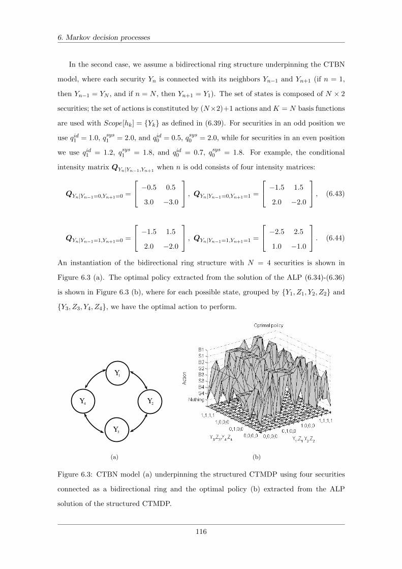
6. Markov decision processes
In the second case, we assume a bidirectional ring structure underpinning the CTBN
model, where each security Yn is connected with its neighbors Yn−1 and Yn+1 (if n = 1,
then Yn−1 = YN , and if n = N , then Yn+1 = Y1). The set of states is composed of N × 2
securities; the set of actions is constituted by (N×2)+1 actions and K = N basis functions
are used with Scope[hk] = {Yk} as defined in (6.39). For securities in an odd position we
use qid1 = 1.0, qsys1 = 2.0, and qid0 = 0.5, qsys0 = 2.0, while for securities in an even position
we use qid1 = 1.2, qsys1 = 1.8, and qid0 = 0.7, qsys0 = 1.8. For example, the conditional
intensity matrix QYn|Yn−1,Yn+1when n is odd consists of four intensity matrices:
QYn|Yn−1=0,Yn+1=0 =
−0.5 0.5
3.0 −3.0
, QYn|Yn−1=0,Yn+1=1 =
−1.5 1.5
2.0 −2.0
, (6.43)
QYn|Yn−1=1,Yn+1=0 =
−1.5 1.5
2.0 −2.0
, QYn|Yn−1=1,Yn+1=1 =
−2.5 2.5
1.0 −1.0
. (6.44)
An instantiation of the bidirectional ring structure with N = 4 securities is shown in
Figure 6.3 (a). The optimal policy extracted from the solution of the ALP (6.34)-(6.36)
is shown in Figure 6.3 (b), where for each possible state, grouped by {Y1, Z1, Y2, Z2} and
{Y3, Z3, Y4, Z4}, we have the optimal action to perform.
Y4 Y2
Y1
Y3
(a) (b)
Figure 6.3: CTBN model (a) underpinning the structured CTMDP using four securities
connected as a bidirectional ring and the optimal policy (b) extracted from the ALP
solution of the structured CTMDP.
116

6. Markov decision processes
6.6 Discussion
After a brief introduction about the basic concepts, we have presented the Markov decision
process framework in factored discrete time and structured continuous time domains and
solved them via approximate linear programming. Both models can scale up to large prob-
lems by exploiting the additive and context-specific structures of complex systems and by
using linear value function approximations. We have discussed differences and similarities
of the two models in a comprehensive vision. A new formulation of a trading problem
in structured continuous time domains has been presented, and different instantiations of
this problem have been implemented and solved.
117
Chapter 7
Model-based reinforcement
learning
Reinforcement learning is a broad area of machine learning that addresses the problem of
how a decision-maker can learn a behavior through trial and error interactions with an
uncertain environment. We focus on the specific area called model-based reinforcement
learning in which the decision-maker uses his experience to construct a model of the
environment. This model can then be used to predict the outcome of the decision-maker’s
actions in order to enhance his learning performance. We start this chapter introducing
the general reinforcement learning framework, we continue describing the model-based
reinforcement learning techniques in factored MDPs and a novel extension to structured
CTMDPs, then we finish analyzing the trading problem discussed in the previous chapter.
7.1 General model
In the standard reinforcement learning model, a decision-maker learns from interactions
with the environment or, in other terms, from repeated simulation. Specifically, at each
interaction, the decision-maker receives the current state of the environment, he chooses
an available action and then he performs it. The action causes the state transition of
the environment and the value of this state transition is revealed to the decision-maker
via a reinforcement signal. The goal of the decision-maker is to find a policy in order to
maximize an expected return over the reinforcement signals (Kaelbling et al., 1996).
118
7. Model-based reinforcement learning
We assume that the current state of the environment is observed (i.e. full observability)
and that the environment is stationary, so that the probabilities of the state transitions,
as well as the corresponding reinforcement signals, do not change over time. We refer to
Bertsekas and Tsitsiklis (1996); Sutton and Barto (1998); Wiering and van Otterlo (2012)
for further material on this framework.
Definition 7.1. Reinforcement learning (RL) model, (Kaelbling et al., 1996). A RL model
consists of a tuple (X,A,S) where: X is a finite set of states; A is a finite set of actions;
S is a set of (bounded) reinforcement signals, where S = {s : s ∈ [0, smax]}.
RL is defined by characterizing a learning problem not a learning method. Thus, any
method that is well suited to solving this problem can be considered a RL method. For
example, when the model of the environment is described as a Markov decision process
and it is known, then dynamic programming methods and linear programming can be
used to solve it. On the contrary, when a model of the environment is not available, then
Monte Carlo methods can be used. These methods require only experiences (samples)
of sequences of states, actions and rewards from on-line or simulated interactions with
the environment. Rather than using a model to compute the value of a given state, they
simply average many returns obtained starting in that state. Unfortunately, the variance
of the returns can be high, which slows convergence (Fishman, 2003).
Reinforcement learning is primarily concerned with how to obtain an optimal policy
when a model of the environment is not known in advance. The decision-maker must
interact with the environment directly to obtain information which can be processed to
produce an optimal policy. At this point he can learn a controller without learning a
model (model-free) or learn a model and use it to derive a controller (model-based).
It is important to note that RL differs from the problem of supervised learning in many
ways. Firstly, there is no presentation of input-output pairs, in fact the RL decision-maker
is not told which actions to take, but he must discover which actions yield the most reward
by trying them. Secondly, it is an interactive problem in which the evaluation of the system
is often concurrent with learning. Thirdly, there is the exploration of the environment,
in fact the RL decision-maker has to exploit what he already knows in order to obtain a
reward, but he also has to explore in order to make better action selections in the future
(Sutton and Barto, 1998; Wiering and Schmidhuber, 1998).
119
7. Model-based reinforcement learning
7.1.1 Exploration versus exploitation
One of the main challenges that arises in reinforcement learning is the trade-off between
exploration and exploitation. The exploration task is performed by an action taken for
the purpose of gathering new information, while the exploitation task is performed by an
action tried in the past and found to be effective in producing rewards. In order to receive
a near-optimal return, a balance between these two types of actions must be achieved.
There are different exploration heuristics used in RL; we present the most used ones
(Thrun, 1992). The simplest action selection strategy is called e-greedy, and it consists
of selecting the greedy action by default, but with probability e to choose an action at
random from a uniform distribution. There are some variants of this strategy that start
with a large value of e to encourage initial exploration and then slowly decrease, such as
the Boltzmann exploration. If the parameter of e-greedy is made a function of time and
the resulting sequence is tuned with care, then it can be made competitive with more
sophisticated strategies. However, the best choice is problem dependent, and there is not
a general way of obtaining good results with e-greedy and its variants (Auer et al., 2002).
Another action selection strategy is optimism in the face of uncertainty in which ac-
tions are selected greedily, but strongly optimistic prior beliefs are put to their payoffs
so that strong negative evidences are used to discard actions (Lai and Robbins, 1985).
Many RL techniques use this idea, such as the exploration bonus in dyna (Sutton, 1990),
curiosity-driven exploration (Schmidhuber, 1991) and the exploration mechanism in prior-
itized sweeping (Moore and Atkeson, 1993). Actions can be also chosen based on interval
estimation (Kaelbling, 1993); in this case, the number of successes and the number of trials
are used to construct confidence intervals on the success probability of each action.
There are algorithms which define unique optimal solutions. Bayesian reinforcement
learning provides an optimal solution in the Bayesian context by taking all possible models
weighted by their posteriors into account at once (Poupart et al., 2006; Kolter and Ng,
2009). An alternative approach is provided by the probabilistically approximately correct
(PAC-MDP) framework for model-based reinforcement learning methods (Kakade, 2003).
The seminal algorithms E3 (Kearns and Singh, 1998) and R-max (Brafman and Tennen-
holtz, 2001) execute near-optimal actions in all but a polynomial number of steps. We
will discuss some advances of these algorithms in the next sections.
120
7. Model-based reinforcement learning
7.1.2 Model-free methods
Temporal-difference methods are suitable for solving the reinforcement learning problem;
they combine the Monte Carlo idea, as they learn from experience without a model of
the environment, and the dynamic programming idea, as they bootstrap, i.e. they update
estimates from previous estimates without waiting for the final outcome. The general idea
of temporal-difference algorithms can be explained as follows. Consider an experience
(x, a, s,x′) summarizing a single transition of the environment, where x is the decision-
maker’s state before the transition, a is his choice of action, s is the reinforcement signal
received and x′ is the resulting state. The update rule of the value function in the case of
discounted return is:
V (x) = (1− η)V (x) + η(s+ γV (x′)), (7.1)
where η is the learning rate. The key idea is that s + γV (x′) is a sample of the value of
V (x) and it is likely to be correct because of the incorporation of the reinforcement signal
s. If the learning rate η is slowly decreased and the policy is held fixed, then the temporal-
difference converges to the optimal value function (Sutton, 1988). A generalization of this
algorithm applies the update rule (7.1) to every state according to its eligibility rather
than just to the immediately previous state. This generalization is computationally more
expensive, but it often converges faster (Dayan, 1992).
Probably one of the best known temporal-difference algorithms is Q-Learning (Watkins,
1989; Watkins and Dayan, 1992). It is an off-policy method because it learns the value
of the optimal policy independently of the decision-maker’s actions. In order to illustrate
Q-Learning, we have to introduce some additional notation. For control purposes, rather
than the value of each state, it is easier to consider the value of each action in each state.
Let Q(x, a) be the expected return starting from state x, taking action a, and then fol-
lowing the actual policy. In this case we have that V ∗(x) = maxaQ∗(x, a). Note that
we are assuming that both states and actions are finite, and they can be stored explic-
itly in a lookup table. Since the Q function makes the action explicit, we can estimate
the Q values online using essentially the same update rule (line 6 of Algorithm 7.1) as
temporal-difference:
Q(x, a) = (1− η)Q(x, a) + η(s+ γmaxa′
Q(x′, a′)). (7.2)
121

7. Model-based reinforcement learning
Under the assumption that every state-action pair is visited infinitely often and ap-
propriate learning rates are used, the Q values converge to Q∗ (Jaakkola et al., 1994b).
Q-Learning can also be adapted in the case of average return (Schwartz, 1993) and conver-
gence properties can be guaranteed (Jaakkola et al., 1994a). When the state and action
spaces become very large, i.e. they cannot be stored in a lookup table anymore, then
some generalizations of Q-Learning have been introduced. For example, function approx-
imation techniques have been used, but few convergence results under rather restrictive
conditions have been proved (Melo et al., 2008). State aggregation techniques have been
also introduced, for example interpolation based Q-Learning has been proved to converge
if the assumption about the interpolation property is satisfied (Szepesvari and Smart,
2004). Another strategy for dealing with large state spaces is to treat them as hierarchical
problems, this strategy introduces slight sub-optimality in performance, but potentially
gain a good efficiency in learning time and space (Barto and Mahadevan, 2003).
Another well known temporal-difference algorithm is SARSA (Rummery and Niranjan,
1994). Unlike Q-Learning, it is an on-policy method because it learns the value of the policy
being carried out by the decision-maker including the exploration steps. The update rule is
given in line 7 of Algorithm 7.2. As Q-Learning, it has been proved to converge to optimal
values (Singh et al., 2000). In some cases, such as in the case of function approximations,
an on-policy algorithm like SARSA can be more effective than Q-Learning (Gosavi, 2009).
Algorithm 7.1 Q-Learning (tabular)
Require: learning rate η > 0.
Ensure: optimal Q function Q∗.
1: Initialize Q(x, a) ∀x ∈X, ∀a ∈ A2: x← startingState()
3: repeat
4: a← chooseAction(x, Q)
5: (s,x′)←takeAction(a)
6: Q(x, a)← (1− η)Q(x, a) +
η(s+ γmaxa′ Q(x′, a′))
7: x← x′
8: until (isTerminal(x))
Algorithm 7.2 SARSA (tabular)
Require: learning rate η > 0.
Ensure: optimal Q function Q∗.
1: Initialize Q(x, a) ∀x ∈X, ∀a ∈ A2: x← startingState()
3: a← defaultAction()
4: repeat
5: (s,x′)← takeAction(a)
6: a′ ← chooseAction(x′, Q)
7: Q(x, a)← (1− η)Q(x, a) +
η(s+ γQ(x′, a′))
8: x← x′
9: a← a′
10: until (isTerminal(x))
122
7. Model-based reinforcement learning
7.1.3 Model-based methods
Model-free methods presented in the previous section do not exploit the knowledge of the
environment gathered during exploration. Although many of these methods are guaran-
teed to find optimal policies and use little computation time per experience, they require
a huge amount of data to achieve good performance (Kaelbling et al., 1996). A different
class of reinforcement learning methods, called model-based, do not assume knowledge of
the model of the environment in advance, but they try to learn it from experience.
The simplest model-based RL method is certainty equivalence (Kumar and Varaija,
1986). In this framework, the decision-maker maintains an estimated model of the envi-
ronment as an MDP with transition model P and reward function R. For each experience
(x, a, s,x′), the decision-maker updates the estimated model and solves it to obtain a pol-
icy that would be optimal if the estimated model was true, and he acts according to that
policy. A common approach is to use the empirical distribution of observed state transi-
tions and rewards for the estimated model. For instance, if action a has been attempted
C(x, a) times in state x and on C(x, a,x′) of these times the state x′ has been reached,
then the estimate of true probability P (x′|x, a) is P (x′|x, a) = C(x, a,x′)/C(x, a). If
C(x, a) = 0, then a prior distribution is used (Dearden et al., 1999). The drawbacks of
this method are the continuous interactions with the environment and the computational
burden of resolving the model for each update of P and R.
A common solution to speed up the learning procedure is provided by the dyna frame-
work (Sutton, 1990). The key idea is to use the acquired experience to construct a model of
the environment and then use it for updating the value function without having to interact
with the environment. This updating is performed in the same spirit of temporal-difference
algorithms, e.g. using the equation (7.2), but for a limited number of iterations.
Several variations of dyna have been developed to improve its performance, such as
prioritized sweeping (Moore and Atkeson, 1993). This approach does not uniformly select
the state-action pairs to update equation (7.2), but it focuses on state-action pairs that
are likely to be useful. As shown in Algorithm 7.3, a priority queue is maintained for every
state-action pair whose estimated value would change substantially if backed up, ordered
by the size of the change. When the top of the queue is backed up, the effect on each of
its predecessor pairs is computed, so the effects of the changes are propagated backward.
123

7. Model-based reinforcement learning
Algorithm 7.3 Prioritized sweeping
Require: learning rate η > 0, error threshold υ and max number of iterations Itermax.
Ensure: optimal Q function Q∗.
1: Initialize Q(x, a) ∀x ∈X, ∀a ∈ A,model, pQueue.2: x← startingState()
3: repeat
4: a← chooseAction(x, Q)
5: (s,x′)← takeAction(a)
6: model← (x, a, s,x′)
7: err ← |s+ γmaxa′ Q(x′, a′)−Q(x, a)|8: if (err > υ) then
9: pQueue← push(pQueue, (x, a), err)
10: end if
11: i← 0
12: while (pQueue 6= ∅ and i < Itermax) do
13: (x, a)← pop(pQueue)
14: (s, x′)← model(x, a)
15: Q(x, a)← (1− η)Q(x, a) + η(s+ γmaxa′ Q(x′, a′))
16: i← i+ 1
17: for each (x, a, s) predicted by model to lead to x do
18: err ← |s+ γmaxaQ(x, a)−Q(x, a)|19: if (err > υ) then
20: pQueue← push(pQueue, (x, a), err)
21: end if
22: end for
23: end while
24: x← x′
25: until (isTerminal(x))
Extensions of prioritized sweeping to large state space using linear function approxima-
tion has been developed. Specifically, Sutton et al. (2008) have established that dyna-style
planning with reinforcement learning update rules converges under weak conditions. Even
if the idea of prioritized sweeping of focusing search on the states believed to have changed
in value can speed up its convergence, the overhead of managing the priority queue can
be prohibitively high (Wingate and Seppi, 2005; Dai and Hansen, 2007).
124
7. Model-based reinforcement learning
7.2 Model-based RL in factored MDPs
Model-based RL methods are important in applications where computation is considered
to be cheap and real world experience costly as they can speed up their convergence with a
better use of experience. However, they must be able to efficiently manage the exploration-
exploitation trade-off and scale up to large state spaces in order to be successfully used
to solve non trivial problems. In order to deal with these two issues, explicit exploration
strategies have been developed and factored MDPs have been used.
7.2.1 Prioritized sweeping-based algorithms
Generalized prioritized sweeping (Andre et al., 1998) is an extension of prioritized sweeping
with two important contributions: they use a parametrized version of the value function
and a compact representation of the environment by using a factored MDP. Like prioritized
sweeping, their method aims to perform only the most beneficial value propagations. In
particular, when performing value propagations, the decision-maker updates the value
function by updating its parameters. In order to estimate the change in the Bellman
error without computing it for each state, they use the gradient of the Q function. For
the environment representation, they assume that the DBNs structures underpinning the
factored MDP model are given, and they learn the conditional probability entries using
Dirichlet priors for each multinomial distribution.
Structured prioritized sweeping (Dearden, 2001) is an extension of generalized priori-
tized sweeping in which the factored MDP is represented by DBNs with tree-structured
conditional probability tables. This algorithm maintains a structured value function and
updates the values of aggregate states. It applies the techniques used in the structured pol-
icy iteration algorithm (Boutilier et al., 1995), such as the regression operator computed
in a structured way where the value function is represented as a tree and the result is
another tree in which each leaf corresponds to a region of the state space. An advantage
of this algorithm is that the DBNs structure can be unknown.
Both generalized prioritized sweeping and structured prioritized sweeping take advan-
tage of the structure of the factored MDP to improve learning, but they do not take into
account the issue of exploration in such domains.
125

7. Model-based reinforcement learning
7.2.2 Factored E3
The E3 algorithm (Kearns and Singh, 1998) is a model-based RL method that provides
an explicit handling of the exploration-exploitation trade-off. As the certainty equivalence
method, E3 keeps an estimated model of the environment as an MDP that is updated
during execution. Upon arriving in a state it has never visited before, it takes an arbitrary
action, otherwise it takes the action it has tried the fewest times from that state.
A key notion of E3 is that of known-state MDP, that is an MDP where all transitions
between known states are preserved, while all other transitions are redirected to an absorb-
ing state that represents all of the unknown and unvisited states. This known-state MDP
is not directly accessible to the algorithm, but it is possible to have a good approximation
of it according to the simulation lemma introduced by Kearns and Singh (1998). The au-
thors also defined the explore or exploit lemma, which formalizes that either the optimal
(T -step) policy achieves its high return by staying, with high probability, in the set of cur-
rently known states (so it can perform exploitation), or the optimal policy has significant
probability of leaving the currently known states within T steps (so it can perform explo-
ration that quickly reaches the absorbing state). Thus, by performing two polynomial-time
computations on the known-state MDP off-line, the algorithm is guaranteed to either find
a way to get near-optimal return or find a way to improve its estimates.
The E3 algorithm makes no assumptions about the structure of the MDP, so the
resulting polynomial dependence on the number of states makes E3 impractical in the
case of large MDPs. Kearns and Koller (1999) derived a generalization of E3, called
factored E3, where the underlying model can be represented as a factored MDP in which
the structure is known, but the parameters are unknown. In their work, the concept of
known-state is extended to the idea of known-transition, that is known if all of its CPT
entries of the underlying DBN are known. The core part of factored E3 is essentially the
same as of that E3. After some number of steps, one or more transitions become known by
the Pigeonhole principle (Fletcher and Patty, 1995). When it reaches a known state (one
where all the transitions are known), it performs approximate off-line policy computations
for two different factored MDPs. The first corresponds to attempted exploitation and the
second to attempted exploration. Factored E3 has a polynomial dependence not on the
number of states, but on the number of CPT parameters in the factored MDP.
126
7. Model-based reinforcement learning
7.2.3 Factored R-max
R-max is a more general algorithm than E3, which can attain near-optimal return in poly-
nomial time (Brafman and Tennenholtz, 2001). It uses the idea of certainty equivalence
as the decision-maker maintains a complete, but possibly inaccurate model of the environ-
ment and acts based on the optimal policy derived from this model. The action selection
strategy follows the optimism in the face of uncertainty principle. In particular, the ac-
tion selection step is always to choose the action that maximizes the current action value,
maxaQ(x, a), while the model update step is to solve the following set of equations:
Q(x, a) =
R(x, a) + γ
∑x′ P (x′|x, a) maxa′ Q(x′, a′) if C(x, a) ≥ c,
Rmax otherwise,
(7.3)
where R(x, a) and P (x′|x, a) are the empirical estimates for the reward and transition dis-
tribution of state-action pair (x, a) using only data from the first c counts of (x, a). Strehl
et al. (2009) demonstrated that c can be defined as a function of the input parameters in
the PAC-MDP framework in order to make theoretical guarantees about its efficiency.
Any implementation of R-max must choose a technique for solving the set of equations
(7.3) such as dynamic programming and linear programming. Following the generalization
of E3 to factored E3, Guestrin et al. (2002) introduced the factored R-max in which the
environment is modeled as a factored MDP and solved (7.3) using the approximate linear
programming approach (6.17)-(6.19). Strehl (2007) proposed a similar algorithm that
takes into account the empirical estimates for the transition components.
Different extensions of the R-max algorithm have been introduced that do not assume
knowledge of the structure of the factored MDP in advance. Strehl et al. (2007) pro-
posed SLF-R-max that learns the structure as part of the reinforcement learning process
requiring as input only an upper bound in-degrees of the underlying DBN. It behaves
near optimally, with high probability, in all but a polynomial number of time steps. The
sample complexity of this algorithm has been improved by Diuk et al. (2009) with their
Met-R-max. Chakraborty and Stone (2011) studied the case when a prior knowledge in-
degrees of the underlying DBN is unavailable for an ergodic factored MDP. Given a big
enough time T , their LSE-R-max algorithm provably achieves a return sufficiently close
to the optimal one with high certainty and polynomial complexity.
127
7. Model-based reinforcement learning
7.2.4 Algorithm-directed factored reinforcement learning
Both factored E3 and factored R-max suffer from some limitations, e.g. the concept of
known state is quite limiting, given that many visits are required before a state becomes
relevant to the plan. Guestrin et al. (2002) proposed an alternative approach, called
algorithm-directed factored reinforcement learning, that uses an ALP as planning algo-
rithm. Their approach only learns the critical parts of the model needed for the ALP and
it achieves a sample efficiency which is logarithmic in the size of the problem description.
They assumed that the decision-maker is interested in maximizing the infinite-horizon av-
erage return ρ and is trying to obtain a linear approximation of the optimal value function
using the average return version of the ALP (6.17)-(6.19) defined as follows:
vars : ρ, w1, . . . , wK (7.4)
min : ρ (7.5)
s.t. : 0 ≥ maxx
{−ρ+R(x, a) +
K∑k=1
wk (gak(x)− hk(x))
}, ∀a ∈ A. (7.6)
They defined an ε-optimal algorithm-directed approximation as a factored MDP which
yields |ρ∗alp− ρ| < ε, for some ε > 0, where ρ∗alp is the exact-model average return obtained
by solving the ALP (7.4)-(7.6) with the true-model, while ρ is the estimated-model average
return obtained by solving the same ALP with the estimates P (x′|x, a) and R(x, a).
The key idea of their approach is the construction of two ALPs (7.4)-(7.6), one uses all
lower bounds on reward functions and backprojections, and it provides a solution ρ, while
the other one uses all upper bounds on the same functions and returns a solution ρ. These
bounds are updated during execution and they are constructed such that ρ ≤ ρ∗alp ≤ ρ with
probability at least (1 − αρ). Both lower ρ and upper ρ solutions are important because
they provide two types of information: a stopping criterion ρ − ρ < ε, in order to obtain
an ε-optimal algorithm-directed approximation, and which states need to be explored to
make the bounds tighter, i.e. the active states of the two ALPs.
As factored R-max, this algorithm assumes that the structure of the factored MDP
is known. During execution, it maintains lower and upper bounds on reward functions
and backprojections. After solving the two ALPs described above, it verifies whether the
stopping criterion has been reached. If not, it collects the active state-action pairs of the
two ALPs and it drives the exploration toward the relevant active states.
128

7. Model-based reinforcement learning
7.3 Model-based RL using structured CTMDPs
Model-based reinforcement learning algorithms using factored MDPs have been used to
scale up to large state spaces and techniques to solve them have been widely developed.
However, when the system does not evolve natively in discrete time, it is necessary to
resort to some forms of discretization, leading to the same problems incurred in DBNs.
We present a novel model-based reinforcement learning approach for control continuous
time dynamic systems based on structured CTMDPs (Villa and Shelton, 2014a). Our
approach extends the algorithm-directed factored RL in the continuous time case allowing
us to manage the exploration-exploitation trade-off via an ad-hoc ALP formulation for
infinite-horizon average return in continuous time. We also maintain a sample efficiency
logarithmic in the size of the problem description.
7.3.1 Approximate linear program
As we are interested in maximizing the infinite-horizon average return, we have to derive
the ALP formulation for structured CTMDPs in this case. This task can be accomplished
in the same way as the infinite-horizon discounted return, where we derived the ALP
formulation from that of factored MDPs.
Recall the set of constraints (6.12) of the ALP formulation for discounted return in
discrete time and the Bellman optimality operator (6.25) in continuous time for average
return. Then, the set of constraints for average return can be written as follows:
ρ
qax+
K∑k=1
wkhk(x) ≥ r(x, a)
qax+∑x′ 6=x
qax,x′
qax
K∑k=1
wkhk(x′), ∀x ∈X,∀a ∈ A. (7.7)
By multiplying both sides of the inequality (7.7) by qax, moving everything from the left
hand side to the right hand side and rearranging, we obtain the following set of constraints:
0 ≥ −ρ+ r(x, a) +K∑k=1
wk(−qaxhk(x) +∑x′ 6=x
qax,x′hk(x′)), ∀x ∈X, ∀a ∈ A. (7.8)
Given that only one single variable changes state at any single instant (6.31) and the rate
at which a variable transitions is independent of all the other variables given the values of
the parents, then the inequality (7.8) can be simplified ∀x ∈X,∀a ∈ A as follows:
0 ≥ −ρ+ r(x, a) +K∑k=1
wk(∑
Xn∈Ck
∑x′n 6=xn
qaxn,x′n|pau(hk(x[x′n])− hk(x))). (7.9)
129
7. Model-based reinforcement learning
Then, the ALP for infinite-horizon average return in structured CTMDPs is defined as:
vars : ρ, w1, . . . , wK (7.10)
min : ρ (7.11)
s.t. : 0 ≥ maxx
{−ρ+
L∑l=1
rl(x, a) +K∑k=1
wkgak(x)
}, ∀a ∈ A, (7.12)
where we use the max operator to combine the constraints (7.9) for the same action a,
while gak is the backprojection of the k-th basis function hk for action a as defined in
equation (6.37) with Scope[gak ] = Bak ⊆X. The reward rate function is composed of a set
of L localized functions, r(x, a) =∑L
l=1 rl(Lal , a) ∈ [0;Rlmax ] with Scope[rl] = Lal ⊆X.
Given a set of basis functions H = {h1, . . . , hK} where 0 ≤ hk(x) ≤ Hmax, ∀k,x, and
a model defined as a structured CTMDP, it is possible to solve the ALP (7.10)-(7.12) and
obtain the continuous time version of the exact-model average return ρ∗alp. In the context
of RL, the conditional intensities as well as the reward rate functions of the structured
CTMDP are unknown. We are interested in estimating them and providing an ε-optimal
algorithm-directed approximation of the exact-model as in Guestrin et al. (2002).
7.3.2 Lower and upper bounds
The main part of the algorithm is to provide lower ρ and upper ρ bounds on the exact-
model average return such that:
P (ρ ≤ ρ∗alp ≤ ρ) ≥ (1− αρ). (7.13)
As first step, we would like to maintain lower and upper bounds on the unknown compo-
nents in (7.12), namely the reward rate functions rl(x, a) and backprojections gak(x).
Given an experience occurred along the path χ = ((t,x), a, s(x, a), (t′,x[x′n])) where
only the variable Xn has changed its state, if Xn ∈ Lal , then it can be used to estimate
the local reward rate function as follows:
rl(x, a) =1
C(χlal )
∑χlal
s(x, a)−√
R2lmax
2C(χlal )ln
(2L|A||Lmax|
αr
), (7.14)
rl(x, a) =1
C(χlal )
∑χlal
s(x, a) +
√R2lmax
2C(χlal )ln
(2L|A||Lmax|
αr
), (7.15)
130
7. Model-based reinforcement learning
where χlal denotes the experience where the state x is consistent with lal and C(χlal ) is
the number of such experiences. If C(χlal ) = 0, then rl(x, a) = 0 and rl(x, a) = Rlmax .
Given that there are L localized functions for |A| actions with at most |Lmax| assignments
each, where |Lmax| is the maximum reward rate function scope size |Lmax| = maxx,l |Lal |,
the entire reward rate function can be bounded with probability at least (1− αr) by the
application of Hoeffding and Union bounds, as shown in equations (7.14) and (7.15).
Consider the other component of the set of constraints (7.12), we would like to maintain
lower and upper bounds on the backprojections such that gak(x) ≤ gak(x) ≤ gak(x) holds.
From equation (6.37), we note that each backprojection is essentially an expectation over
a small set of states bak ∈ Bak ⊆ X that yields a backprojected basis reward over time.
We can estimate these bounds by doing an empirical mean computation of the rewards
obtained divided by the empirical mean time of occurrence. Therefore, we introduce two
elements: the mean value gvak(x) and the mean time gt
ak(x) backprojections.
Given an experience occurred along the path χ = ((t,x), a, s(x, a), (t′,x[x′n])) where
only the variable Xn has changed its state, if Xn ∈ Bak, then it can be used to estimate
the two elements of the backprojection gvak(x) and gt
ak(x) as follows:
gvak(x) =
1
C(χbak)
∑χbak
(hk(x[x′n])− hk(x)), (7.16)
gtak(x) =
1
C(χbak)
∑χbak
(t′ − t), (7.17)
where χbak denotes the experience where the state x is consistent with bak and C(χbak)
is the number of such experiences. The lower and upper bounds for the mean value
backprojection which will hold with high probability are: gvak(x) = gv
ak(x) − εgvak and
gvak(x) = gv
ak(x) + εgvak respectively, where the error parameter εgvak is given by:
εgvak =
√2H2
max
C(χbak)ln
(4K|A||Bmax|
αg
). (7.18)
The lower and upper bounds for the mean time backprojection which will hold with high
probability are: gtak(x) = gt
ak(x)− εgtak and gt
ak(x) = gt
ak(x) + εgtak respectively, where the
error parameter εgtak is given by:
εgtak =
√T 2max
2C(χbak)ln
(4K|A||Bmax|
αg
). (7.19)
131

7. Model-based reinforcement learning
The errors reported in (7.18) and (7.19) are constructed such that all backprojections
are bounded with probability at least (1 − αg) by Hoeffding and Union bounds with the
following two assumptions. Firstly, we assume that all the possible differences of the
backprojections (hk(x′)−hk(x)) belong to the interval [−Hmax;Hmax]. Secondly, we also
assume that all the possible time differences (t′ − t) are in the interval [0;Tmax]. The
Union bound is used since there are 2 elements for K basis functions for |A| actions with
at most |Bmax| assignments each, where |Bmax| is the maximum backprojection scope
size |Bmax| = maxx,k |Bak|. The lower and the upper bounds on the backprojections can
be then computed using the rule of uncertainty propagation (Taylor, 1996) as follows:
gak(x) =
gvak
gtak
1−√(
εgvakgvak
)2
+
(εgtakgtak
)2 , (7.20)
gak(x) =gvak
gtak
1 +
√(εgvakgvak
)2
+
(εgtakgtak
)2 . (7.21)
As second step, we show that the proposed bounds on reward rate functions and
backprojections can be used to ensure that inequality (7.13) holds.
Let ρ be the estimated-model average return obtained by solving the ALP (7.10)-(7.12)
using the lower bounds of the reward rate functions rl(x, a) and backprojections gak(x)
and let ρ be the estimated-model average return by solving the same ALP using the upper
bounds of the reward rate functions rl(x, a) and backprojections gak(x). Then, for any
αρ > 0, we have that ρ ≤ ρ∗alp ≤ ρ holds with probability at least (1− αρ).
We can prove this proposition in two parts following the work of Guestrin et al. (2002).
Firstly, we note that all sources of uncertainty of the ALP are bounded with high prob-
ability by construction of the error parameters. Thus, the lower and upper bounds hold
with probability at least (1−αρ) by setting αr = αρ/2 and αg = αρ/2. Secondly, we note
that if we use the lower bounds rl(x, a) and gak(x) instead of true values rl(x, a) and gak(x),
then the feasible region becomes larger, therefore the return ρ∗alp is still feasible. Thus,
using the same set of basis weights as the ones in the solution provided when the model
is known, we can decrease the objective function obtaining a smaller return ρ compared
to ρ∗alp. Similarly, if we replace the upper bounds rl(x, a) and gak(x) with the true values
rl(x, a) and gak(x), then the feasible region becomes smaller, therefore the return ρ∗alp may
not be longer feasible, so the upper bound return ρ cannot be smaller than ρ∗alp.
132
7. Model-based reinforcement learning
7.3.3 Exploration strategy
The lower and upper bounds in (7.13) obtained by solving two ALPs (7.10)-(7.12) using
the lower and upper bounds of the reward rate functions and backprojections give us two
types of information. Firstly, the stopping criterion, i.e. if ρ−ρ < ε, then we have obtained
the ε-optimal approximation with probability at least (1− αρ). Secondly, the exploration
strategy, i.e. which states need to be explored to make the bounds tighter.
These critical states can be found in the solutions of the ALPs. Specifically, a solution
of an ALP problem provides active constraints that correspond to the critical state-action
pairs (x, a) for which the inequality constraints (7.12) become active. If we denote as Prc
the set of state-action pairs with precise backprojections and reward rate functions, i.e.
Prc = {(x, a) : gak(x) = gak(x), rl(x, a) = rl(x, a), ∀k, l}, and all active state-action pairs
of the ALP are in Prc, then its solution is equal to ρ∗alp with probability at least (1−αρ) as
proved by Guestrin et al. (2002). Therefore, the exploration strategy is guided toward the
active states of the ALPs because precise estimates of these states are sufficient to obtain
an ε-optimal approximation. It is important to note that it is not possible to construct the
Prc set in practice because of the uncertainty of the bounds; thus, we have to rely on LP
sensitivity analysis to determine error bars for which small changes in the backprojections
and reward rate functions do not impact the ALP solution.
7.3.4 Algorithm
The algorithm-directed reinforcement learning approach for structured CTMDPs is shown
in Algorithm 7.4. As in factored R-max, we assume that the structure of the structured
CTMDP is given, but its parameters are unknown; moreover, we require a value ε > 0, a
confidence level of (1 − αρ) and a set of basis functions H. The result is a near-optimal
policy π∗ obtained as an ε-optimal algorithm-directed approximation of the exact-model.
During execution, the algorithm maintains two models, denoted as models, that con-
tain the lower and upper bounds on the reward rate functions and the backprojections.
For each experience occurred along the path, the algorithm updates these models and
solves the relative ALPs defined in (7.10)-(7.12), (lines 6 - 7 of Algorithm 7.4). If the
stopping criterion is not met, then the active states of the two ALPs are collected. These
active states are crucial given that their exploration makes the ALPs bounds tighter.
133
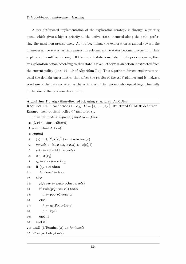
7. Model-based reinforcement learning
A straightforward implementation of the exploration strategy is through a priority
queue which gives a higher priority to the active states incurred along the path, prefer-
ring the most non-precise ones. At the beginning, the exploration is guided toward the
unknown active states; as time passes the relevant active states become precise until their
exploration is sufficient enough. If the current state is included in the priority queue, then
an exploration action according to that state is given, otherwise an action is extracted from
the current policy (lines 14 - 19 of Algorithm 7.4). This algorithm directs exploration to-
ward the domain uncertainties that affect the results of the ALP planner and it makes a
good use of the data collected as the estimates of the two models depend logarithmically
in the size of the problem description.
Algorithm 7.4 Algorithm-directed RL using structured CTMDPs
Require: ε > 0, confidence (1− αρ), H = {h1, . . . , hK}, structured CTMDP definition.
Ensure: near-optimal policy π∗ and error ερ.
1: Initialize models, pQueue, finished← false.
2: (t,x)← startingState()
3: a← defaultAction()
4: repeat
5: (s(x, a), (t′,x[x′n]))← takeAction(a)
6: models← ((t,x), a, s(x, a), (t′,x[x′n]))
7: sols← solveALP(models)
8: x← x[x′n]
9: ερ ← sols.ρ− sols.ρ10: if (ερ < ε) then
11: finished← true
12: else
13: pQueue← push(pQueue, sols)
14: if (isIn(pQueue,x)) then
15: a← pop(pQueue,x)
16: else
17: π ← getPolicy(sols)
18: a← π(x)
19: end if
20: end if
21: until (isTerminal(x) or finished)
22: π∗ ← getPolicy(sols)
134
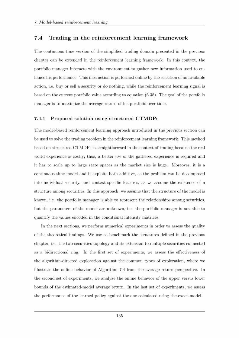
7. Model-based reinforcement learning
7.4 Trading in the reinforcement learning framework
The continuous time version of the simplified trading domain presented in the previous
chapter can be extended in the reinforcement learning framework. In this context, the
portfolio manager interacts with the environment to gather new information used to en-
hance his performance. This interaction is performed online by the selection of an available
action, i.e. buy or sell a security or do nothing, while the reinforcement learning signal is
based on the current portfolio value according to equation (6.38). The goal of the portfolio
manager is to maximize the average return of his portfolio over time.
7.4.1 Proposed solution using structured CTMDPs
The model-based reinforcement learning approach introduced in the previous section can
be used to solve the trading problem in the reinforcement learning framework. This method
based on structured CTMDPs is straightforward in the context of trading because the real
world experience is costly; thus, a better use of the gathered experience is required and
it has to scale up to large state spaces as the market size is huge. Moreover, it is a
continuous time model and it exploits both additive, as the problem can be decomposed
into individual security, and context-specific features, as we assume the existence of a
structure among securities. In this approach, we assume that the structure of the model is
known, i.e. the portfolio manager is able to represent the relationships among securities,
but the parameters of the model are unknown, i.e. the portfolio manager is not able to
quantify the values encoded in the conditional intensity matrices.
In the next sections, we perform numerical experiments in order to assess the quality
of the theoretical findings. We use as benchmark the structures defined in the previous
chapter, i.e. the two-securities topology and its extension to multiple securities connected
as a bidirectional ring. In the first set of experiments, we assess the effectiveness of
the algorithm-directed exploration against the common types of exploration, where we
illustrate the online behavior of Algorithm 7.4 from the average return perspective. In
the second set of experiments, we analyze the online behavior of the upper versus lower
bounds of the estimated-model average return. In the last set of experiments, we assess
the performance of the learned policy against the one calculated using the exact-model.
135
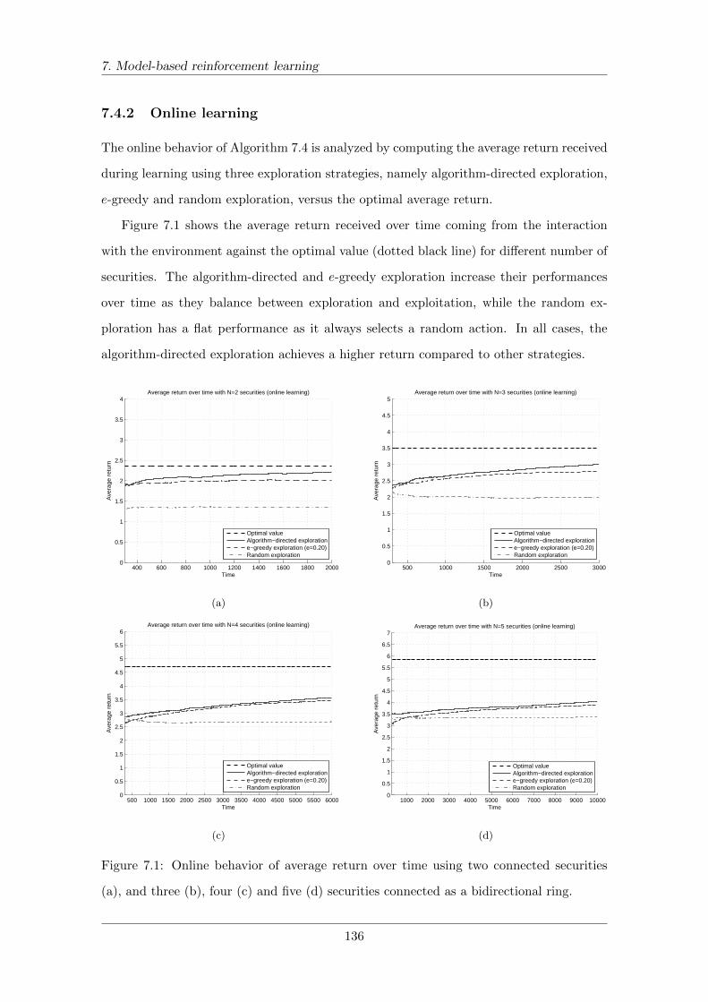
7. Model-based reinforcement learning
7.4.2 Online learning
The online behavior of Algorithm 7.4 is analyzed by computing the average return received
during learning using three exploration strategies, namely algorithm-directed exploration,
e-greedy and random exploration, versus the optimal average return.
Figure 7.1 shows the average return received over time coming from the interaction
with the environment against the optimal value (dotted black line) for different number of
securities. The algorithm-directed and e-greedy exploration increase their performances
over time as they balance between exploration and exploitation, while the random ex-
ploration has a flat performance as it always selects a random action. In all cases, the
algorithm-directed exploration achieves a higher return compared to other strategies.
400 600 800 1000 1200 1400 1600 1800 20000
0.5
1
1.5
2
2.5
3
3.5
4
Time
Ave
rage
ret
urn
Average return over time with N=2 securities (online learning)
Optimal valueAlgorithm−directed exploratione−greedy exploration (e=0.20)Random exploration
(a)
500 1000 1500 2000 2500 30000
0.5
1
1.5
2
2.5
3
3.5
4
4.5
5
Time
Ave
rage
ret
urn
Average return over time with N=3 securities (online learning)
Optimal valueAlgorithm−directed exploratione−greedy exploration (e=0.20)Random exploration
(b)
500 1000 1500 2000 2500 3000 3500 4000 4500 5000 5500 60000
0.5
1
1.5
2
2.5
3
3.5
4
4.5
5
5.5
6
Time
Ave
rage
ret
urn
Average return over time with N=4 securities (online learning)
Optimal valueAlgorithm−directed exploratione−greedy exploration (e=0.20)Random exploration
(c)
1000 2000 3000 4000 5000 6000 7000 8000 9000 100000
0.5
1
1.5
2
2.5
3
3.5
4
4.5
5
5.5
6
6.5
7
Time
Ave
rage
ret
urn
Average return over time with N=5 securities (online learning)
Optimal valueAlgorithm−directed exploratione−greedy exploration (e=0.20)Random exploration
(d)
Figure 7.1: Online behavior of average return over time using two connected securities
(a), and three (b), four (c) and five (d) securities connected as a bidirectional ring.
136
7. Model-based reinforcement learning
7.4.3 Online behavior of lower and upper bounds
The online behavior of the lower ρ and upper ρ bounds of the estimated-model average
return is assessed by computing the relative difference ερ = ρ− ρ over time.
Figure 7.2 shows the temporal evolution of ερ with α = 0.05 for different numbers
of securities using the algorithm-directed exploration strategy. Increasing the number of
securities leads to a higher difference of the two estimated-model average returns in the
first stages and a slower convergence, logarithmically in the size of the problem description.
200 400 600 800 1000 1200 1400 1600 1800 20000
1
2
3
4
5
6
7
8
Time
ε ρ=
ρ−
ρ
Evolution of upper and lower bounds with N=2 securities (online learning)
Algorithm−directed exploration
(a)
500 1000 1500 2000 2500 30000
2
4
6
8
10
12
14
16
Time
ε ρ=
ρ−
ρ
Evolution of upper and lower bounds with N=3 securities (online learning)
Algorithm−directed exploration
(b)
500 1000 1500 2000 2500 3000 3500 4000 4500 5000 5500 60002
4
6
8
10
12
14
16
18
20
Time
ε ρ=
ρ−
ρ
Evolution of upper and lower bounds with N=4 securities (online learning)
Algorithm−directed exploration
(c)
1000 2000 3000 4000 5000 6000 7000 8000 9000 1000012
14
16
18
20
22
24
Time
ε ρ=
ρ−
ρ
Evolution of upper and lower bounds with N=5 securities (online learning)
Algorithm−directed exploration
(d)
Figure 7.2: Online behavior of lower and upper bounds of the estimated-model average
return over time using two connected securities (a), and three (b), four (c) and five (d)
securities connected as a bidirectional ring.
137
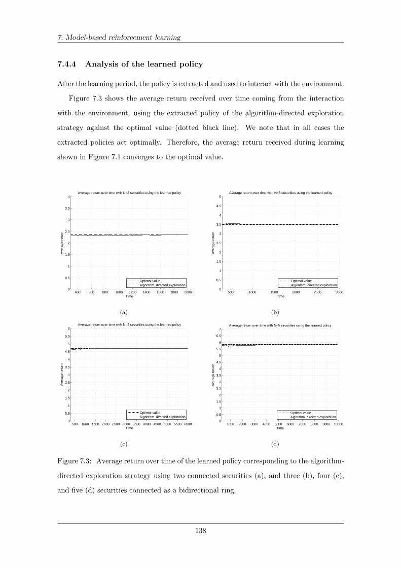
7. Model-based reinforcement learning
7.4.4 Analysis of the learned policy
After the learning period, the policy is extracted and used to interact with the environment.
Figure 7.3 shows the average return received over time coming from the interaction
with the environment, using the extracted policy of the algorithm-directed exploration
strategy against the optimal value (dotted black line). We note that in all cases the
extracted policies act optimally. Therefore, the average return received during learning
shown in Figure 7.1 converges to the optimal value.
400 600 800 1000 1200 1400 1600 1800 20000
0.5
1
1.5
2
2.5
3
3.5
4
Time
Ave
rage
ret
urn
Average return over time with N=2 securities using the learned policy
Optimal valueAlgorithm−directed exploration
(a)
500 1000 1500 2000 2500 30000
0.5
1
1.5
2
2.5
3
3.5
4
4.5
5
Time
Ave
rage
ret
urn
Average return over time with N=3 securities using the learned policy
Optimal valueAlgorithm−directed exploration
(b)
500 1000 1500 2000 2500 3000 3500 4000 4500 5000 5500 60000
0.5
1
1.5
2
2.5
3
3.5
4
4.5
5
5.5
6
Time
Ave
rage
ret
urn
Average return over time with N=4 securities using the learned policy
Optimal valueAlgorithm−directed exploration
(c)
1000 2000 3000 4000 5000 6000 7000 8000 9000 100000
0.5
1
1.5
2
2.5
3
3.5
4
4.5
5
5.5
6
6.5
7
Time
Ave
rage
ret
urn
Average return over time with N=5 securities using the learned policy
Optimal valueAlgorithm−directed exploration
(d)
Figure 7.3: Average return over time of the learned policy corresponding to the algorithm-
directed exploration strategy using two connected securities (a), and three (b), four (c),
and five (d) securities connected as a bidirectional ring.
138

7. Model-based reinforcement learning
7.5 Discussion
We have presented the basic theory about reinforcement learning, a framework that ad-
dresses the problem of how a decision-maker can learn a behavior through interactions
with an uncertain environment. We have discussed the two main methods used to solve
a reinforcement learning problem, namely model-free and model-based, highlighting ad-
vantages and disadvantages. We have described how factored MDPs are exploited to
manage efficiently the exploration-exploitation trade-off and to effectively scale up to
large state spaces in the discrete time settings. We have introduced a novel extension
of model-based methods to control continuous time dynamic systems based on structured
CTMDPs. This approach leverages on an approximate linear program to efficiently man-
age the exploration-exploitation trade-off. It learns the critical parts of the model needed
to solve the approximate linear program and it achieves a sample efficiency which is log-
arithmic in the size of the problem description. The proposed approach has performance
guarantees in the probably approximately correct framework. Finally, the experimental
results on the trading problem have demonstrated the effectiveness of this algorithm.
139
Chapter 8
Conclusions
This thesis has introduced probabilistic graphical models, specifically Bayesian networks,
continuous time Bayesian networks and their extensions, for reasoning and decision-making
in finance. Theoretical findings, applications and path-breaking examples have demon-
strated their effectiveness and they have opened a substantial amount of potential future
work both from theoretical and practical point of views.
8.1 Brief summary
In the first part of this thesis, we have exploited the interplay between modern portfolio
theory and Bayesian networks to propose a novel framework for portfolio analysis and
optimization. It integrates the investor’s market views with a quantitative factor model
and it allows efficient evidential reasoning to understand the behavior of the investment
portfolio in different economic scenarios. We have described continuous time Bayesian
networks, a robust modeling language for structured stochastic processes that evolve over
continuous time. We have highlighted advantages and disadvantages of these models, and
we have given some insights about their use to tackle real financial problems.
In second part of this thesis, we have presented two extensions of continuous time
Bayesian networks to enhance their expressive power and usability: continuous time
Bayesian network classifiers, that allow to perform temporal classification in continuous
time, and non-stationary continuous time Bayesian networks, that allow to represent de-
pendencies which change over time. We have shown how to learn these classifiers from
140
8. Conclusions
Big Data, how to apply them to the foreign exchange rate prediction problem in high
frequency domain and how to use non-stationary continuous time Bayesian networks to
effectively analyze time-series data.
In the last part of this thesis, we have focused on structured continuous time Markov
decision processes that leverage on continuous time Bayesian networks to represent large
and structured continuous time systems. We have provided techniques to solve them
based on linear programming approximation. Finally, we have introduced a model-based
reinforcement learning algorithm to control these systems. It leverages on an approximate
linear program to manage the exploration-exploitation trade-off and it achieves a sample
efficiency, which is logarithmic in the size of the problem description.
8.2 Future directions
Different directions of the future research will focus on both theoretical and practical
challenges. From the theoretical side, we mention the extension of both continuous time
Bayesian network classifiers and non-stationary continuous time Bayesian networks to cope
with hidden nodes, as well as to handle with missing data. Another issue is related to
the design of learning algorithms for continuous time Bayesian networks that can scale
well in distributed processing environment for complete and incomplete data. The solu-
tion of structured continuous time Markov decision processes, as well as the model-based
reinforcement learning algorithm based on them, strongly relies on the efficiency of the ap-
proximate linear program. Therefore, the performance can be increased with the design of
enhanced versions of this algorithm, such as a clever design of the separation oracle used
in the cutting plane algorithm. Moreover, structured continuous time Markov decision
processes can be enriched with the modeling of instantaneous rewards for transitioning
from one state to another.
From the practical side, the analysis of financial data using continuous time Bayesian
networks and their extensions is just at early stages, but there are many possible appli-
cations, ranging from scenario analysis, prediction, time-series analysis, optimization of
distributions over time, to the design of optimal policies in complex trading environments.
This will open the doors to a new way of modeling financial problems.
141
Bibliography
Aalen, O. O., Borgan, O., and Gjessing, H. K. (2008). Survival and Event History Analysis.
Springer.
Acerbi, E. and Stella, F. (2014). Continuous time bayesian networks for gene network
reconstruction: a comparative study on time course data. In The 10th International
Symposium on Bioinformatics Research and Applications (ISBRA 2013), Zhangjiajie,
China.
Ahmed, A. and Xing, E. P. (2009). Recovering time-varying networks of dependencies
in social and biological studies. Proceedings of the National Academy of Sciences,
106(29):11878–11883.
Albanese, C., Jackson, K., and Wiberg, P. (2004). A new fourier transform algorithm for
value at risk. Quantitative Finance, 4(3):328–338.
Andre, D., Friedman, N., and Parr, R. (1998). Generalized prioritized sweeping. Advances
in Neural Information Processing Systems 10, pages 1001–1007.
Andreassen, S., Woldbye, M., Falck, B., and Andersen, S. K. (1987). Munin - a causal
probabilistic network for interpretation of electromyographic findings. In The 10th In-
ternational Joint Conference on Artificial Intelligence (IJCAI-87), Milan, Italy, pages
366–372.
Arnborg, S., Corneil, D. G., and Proskurowski, A. (1987). Complexity of finding embed-
dings in a k-tree. SIAM Journal of Algebraic and Discrete Methods, 8(2):277–284.
Arroyo-Figueroa, G. and Sucar, L. (1999). Temporal bayesian network for diagnosis and
142
Bibliography
prediction. In The 15th Conference on Uncertainty in Artificial Intelligence (UAI 1999),
Stockholm, Sweden, pages 13–20.
Auer, P., Cesa-Bianchi, N., and Fischer, P. (2002). Finite time analysis of the multiarmed
bandit problem. Machine Learning, 47(2-3):235–256.
Barto, A. and Mahadevan, S. (2003). Recent advances in hierarchical reinforcement learn-
ing. Discrete Event Dynamic Systems, 13(1-2):41–77.
Basak, A., Brinster, I., Ma, X., and Mengshoel, O. J. (2012). Accelerating bayesian net-
work parameter learning using hadoop and mapreduce. In The 1st International Work-
shop on Big Data, Streams and Heterogeneous Source Mining (BigMine 12), Beijing,
China, pages 101–108.
Bauerle, N. and Rieder, U. (2011). Markov Decision Processes with Applications to Fi-
nance. Springer-Verlag.
Baviera, R., Pasquini, M., Serva, M., Vergni, D., and Vulpiani, A. (2002). Antipersistent
markov behavior in foreign exchange markets. Physica A, 312(3-4):565–576.
Baviera, R., Vergni, D., and Vulpiani, A. (2000). Markovian approximation in foreign
exchange markets. Physica A, 280(3-4):566–581.
Becker, A. and Geiger, D. (2001). A sufficiently fast algorithm for finding close to optimal
clique trees. Artificial Intelligence, 125(1-2):3–17.
Bellman, R. and Dreyfus, S. (1959). Functional approximation and dynamic programming.
Mathematical Tables and Other Aids to Computation, 13(68):247–251.
Bellman, R. E. (1957). Dynamic Programming. Princeton University Press.
Bertsekas, D. P. (1987). Dynamic Programming: Deterministic and Stochastic Models.
Prentice Hall.
Bertsekas, D. P. and Tsitsiklis, J. N. (1996). Neuro-Dynamic Programming. Athena
Scientific, Belmont, MA.
143

Bibliography
Bertsimas, D., Mersereau, A. J., and Patel, N. R. (2003). Dynamic classification of online
customers. In The 3rd SIAM International Conference on Data Mining (SMD03), San
Francisco, USA.
Bertsimas, D. and Tsitsiklis, J. (1993). Simulated annealing. Statistical Science, 8(1):10–
15.
Berzuini, C. (1989). Representing time in causal probabilistic networks. In The 5th
Conference on Uncertainty in Artificial Intelligence (UAI 1989), Ontario, USA, pages
15–28.
Black, F. and Litterman, R. (1991). Asset allocation: Combining investor views with
market equilibrium. The Journal of Fixed Income, 1(2):7–18.
Boudali, H. and Dugan, J. B. (2006). A continuous-time bayesian network reliability
modeling, and analysis framework. IEEE Transactions on Reliability, 55(1):86–97.
Boutilier, C., Dearden, R., and Goldszmidt, M. (1995). Exploiting structure in policy con-
struction. In The 14th International Joint Conference on Artificial Intelligence (IJCAI-
95), Montreal, Canada.
Boutilier, C., Dearden, R., and Goldszmidt, M. (2000). Stochastic dynamic programming
with factored reppresentations. Artificial Intelligence, 121(1):49–107.
Boutilier, C., T., D., and S., H. (1999). Decision theoretic planning: Structural assump-
tions and computational leverage. Journal of Artificial Intelligence Research, 11:1–94.
Boyen, X. and Koller, D. (1998). Tractable inference for complex stochastic processes.
In The 14th Conference on Uncertainty in Artificial Intelligence (UAI 1998), Madison,
USA.
Brafman, R. I. and Tennenholtz, M. (2001). R-max - a general polynomial time algorithm
for near-optimal reinforcement learning. In The 17th International Joint Conference on
Artificial Intelligence (IJCAI-01), Seattle, USA.
Cerny, V. (1985). Thermodynamical approach to the traveling salesman problem: An effi-
cient simulation algorithm. Journal of Optimization Theory and Applications, 45(1):41–
51.
144
Bibliography
Chakraborty, D. and Stone, P. (2011). Structure learning in ergodic factored mdps without
knowledge of the transition function’s in-degree. In The 28th International Conference
on Machine Learning (ICML 2011), Bellevue, USA.
Cheng, J., Greiner, R., Kelly, J., Bell, D., and Liu, W. (2002). Learning bayesian networks
from data: An information-theory based approach. Artificial Intelligence, 137(1-2):43–
90.
Chickering, D. M., Geiger, D., and Heckerman, D. (1994). Learning bayesian networks is
np-hard. Technical Report MSR-TR-94-17, Microsoft Research.
Chickering, D. M., Geiger, D., and Heckerman, D. (1995). Learning bayesian networks:
Search methods and experimental results. In The 5th International Workshop on Artifi-
cial Intelligence and Statistics (AISTATS 1995), Fort Lauderdale, USA, pages 112–128.
Chinn, M. and Meese, R. (1995). Banking on currency forecasts: How predictable is
change in money? Journal of International Economics, 38:161–178.
Chu, C. T., Kim, S. K., Lin, Y. A., Yu, Y. Y., Bradski, G., Ng, A. Y., and Olukotun,
K. (2006). Map-reduce for machine learning on multicore. In Advances in Neural
Information Processing Systems 19 (NIPS 2006), pages 281–288.
Codecasa, D. and Stella, F. (2014). Learning continuous time bayesian network classifiers.
International Journal of Approximate Reasoning, 55(8):1728–1746.
Cohn, I., El-Hay, T., Kupferman, R., and Friedman, N. (2009). Mean field variational
approximation for continuous-time bayesian networks. In The 25th Conference on Un-
certainty in Artificial Intelligence (UAI 2009), Montreal, Canada.
Condon, A. (1992). The complexity of stochastic games. Information and Computation,
96(2):203–224.
Cooper, G. (1990). Probabilistic inference using belief networks is np-hard. Artificial
Intelligence, 42:393–405.
Dai, P. and Hansen, E. A. (2007). Prioritizing bellman backups without a priority queue.
In The 17th International Conference on Automated Planning and Scheduling (ICAPS-
07), Providence, USA, pages 113–119.
145

Bibliography
Dantzig, G. B. (1963). Linear Programming and Extensions. Princeton University Press.
Darwiche, A. (1995). Conditioning algorithms for exact and approximate inference in
causal networks. In The 11th Conference on Uncertainty in Artificial Intelligence (UAI
1995), Montreal, Canada, pages 99–107.
Dayan, P. (1992). The convergence of td(λ) for general λ. Machine Learning, 8:341–362.
de Campos, L. M., Fernandez-Luna, J. M., and Huete, J. F. (2004). Bayesian networks
and information retrieval: an introduction to the special issue. Information Processing
& Management, 40(5):727–733.
de Farias, D. P. and van Roy, B. (2003). The linear programming approach to approximate
dynamic programming. Operations Research, 51(6):850–865.
de Farias, D. P. and van Roy, B. (2004). On constraint sampling in the linear programming
approach to approximate dynamic programming. Mathematics of Operations Research,
29(3):462–478.
Dean, J. and Ghemawat, S. (2004). Mapreduce: Simplified data processing on large
clusters. In The 6th Conference on Symposium on Opearting Systems Design & Imple-
mentation (OSDI ’04), San Francisco, USA.
Dean, T. and Kanazawa, K. (1989). A model for reasoning about persistence and causation.
Computational Intelligence, 5(2):142–150.
Dearden, R. (2001). Structured prioritised sweeping. In The 18h International Conference
on Machine Learning (ICML 2001), Williamstown, USA, pages 82–89.
Dearden, R., Friedman, N., and Andre, D. (1999). Model-based bayesian exploration. In
The 15th Conference on Uncertainty in Artificial Intelligence (UAI 1999), Stockholm,
Sweden, pages 150–159.
Dechter, R. (1999). Bucket elimination: A unifying framework for reasoning. Artificial
Intelligence, 113(1-2):41–85.
Demirer, R., Mau, R., and Shenoy, C. (2006). Bayesian networks: A decision tool to
improve portfolio risk analysis. Journal of Applied Finance, 16(2):106 – 119.
146
Bibliography
Dempster, M. A. H. and Jones, C. M. (2001). A real-time adaptive trading system using
genetic programming. Quantitative Finance, 1:397–413.
D’Epenoux, F. (1963). A probabilistic production and inventory problem. Management
Science, 10(1):98–108.
Derman, C., Lieberman, G. J., and Ross, S. M. (1975). A stochastic sequential allocation
model. Operations Research, 23(6):1120–1130.
Dimitrova, E. S., Licona, M. P. V., McGee, J., and Laubenbacher, R. (2010). Discretization
of time series data. Journal of Computational Biology, 17(6):853–868.
Diuk, C., Li, L., and Leffler, B. R. (2009). The adaptive k-meteorologists problem and its
application to structure learning and feature selection in reinforcement learning. In The
26th International Conference on Machine Learning (ICML 2009), Montreal, Canada,
pages 249–256.
Domingos, P. and Pazzani, M. (1997). On the optimality of the simple bayesian classifier
under zero-one loss. Machine Learning, 29:103–130.
Dondelinger, F., Lebre, S., and Husmeier, D. (2013). Non-homogeneous dynamic bayesian
networks with bayesian regularization for inferring gene regulatory networks with grad-
ually time-varying structure. Machine Learning, 90(2):191–230.
Duda, R. O. and Hart, P. E. (1973). Pattern Classification and Scene Analysis. John
Wiley & Sons.
Duda, R. O., Hart, P. E., and Stork, D. G. (2000). Pattern Classification. John Wiley &
Sons.
Durante, D. and Dunson, D. B. (2014). Bayesian dynamic financial networks with time-
varying predictors. Statistics & Probability Letters, 93:19–26.
El-Hay, T., Cohn, I., Friedman, N., and Kupferman, R. (2010). Continuous-time belief
propagation. In The 27st International Conference on Machine Learning (ICML 2010),
Haifa, Israel.
147
Bibliography
El-Hay, T., Friedman, N., and Kupferman, R. (2008). Gibbs sampling in factorized
continuous-time markov processes. In The 24th Conference on Uncertainty in Artificial
Intelligence (UAI 2008), Helsinki, Finland, pages 169–178.
Elton, E. J., Gruber, M., Brown, S. J., and Goetzmann, W. N. (2010). Modern Portfolio
Theory and Investment Analysis. John Wiley & Sons, 8th edition.
Fabozzi, F. J., Kolm, P. N., Pachamanova, D., and Focardi, S. M. (2007). Robust Portfolio
Optimization and Management. John Wiley & Sons.
Fagiuoli, E., Omerino, S., and Stella, F. (2008). Mathematical Methods for Knowledge
Discovery and Data Mining, chapter Bayesian Belief Networks for Data Cleaning, pages
204–219. IGI Global.
Fama, E. F. (1965). The behaviour of stock market prices. Journal of Business, 38(1):34–
105.
Fan, Y. and Shelton, C. (2008). Sampling for approximate inference in continuous time
bayesian networks. In The 10th International Symposium on Artificial Intelligence and
Mathematics (ISAIM 2008), Fort Lauderdale, USA.
Fan, Y. and Shelton, C. R. (2009). Learning continuous-time social network dynamics.
In The 25th Conference on Uncertainty in Artificial Intelligence (UAI 2009), Montreal,
Canada.
Fawcett, T. (2006). An introduction to roc analysis. Pattern Recognition Letters,
27(8):861–874.
Fishman, G. (2003). Monte Carlo: Concepts, Algorithms, and Applications. Springer
Series in Operations Research and Financial Engineering. Springer.
Fletcher, P. and Patty, C. W. (1995). Foundations of Higher Mathematics. Cengage
Learning, 3rd edition.
Friedman, N., Geiger, D., and Goldszmidt, M. (1997). Bayesian network classifiers. Ma-
chine Learning, 29(2-3):131–163.
148
Bibliography
Friedman, N. and Koller, D. (2000). Being bayesian about bayesian network structure:
A bayesian approach to structure discovery in bayesian networks. Machine Learning,
50(1-2):95–125.
Friedman, N. and Kupferman, R. (2006). Dimension reduction in singularly perturbed
continuous-time bayesian networks. In The 22nd Conference on Uncertainty in Artificial
Intelligence (UAI 2006), Cambridge, USA.
Friedman, N., Linial, M., Nachman, I., and Pe’er, D. (2000). Using bayesian networks to
analyze expression data. In The 4th Annual International Conference on Computational
Molecular Biology (RECOMB 2000), Tokyo, Japan, pages 127–135.
Gatti, E., Luciani, D., and Stella, F. (2011). A continuous time bayesian network model for
cardiogenic heart failure. Flexible Services and Manufacturing Journal, 24(2):496–515.
Geiger, D. and Heckerman, D. (1997). A characterization of the dirichlet distribution
through global and local parameter independence. Annals of Statistics, 25(3):1344–
1369.
Ghahramani, Z. and Hinton, G. E. (2000). Variational learning for switching state-space
models. Neural Computation, 12(4):963–996.
Giudici, P. and Castelo, R. (2003). Improving markov chain monte carlo model search for
data mining. Machine Learning, 50(1-2):127–158.
Gopalratnam, K., Kautz, K., and Weld, D. S. (2005). Extending continuous time bayesian
networks. In The 20th National Conference on Artificial Intelligence (AAAI-05), Pitts-
burgh, USA.
Gosavi, A. (2009). Reinforcement learning: A tutorial survey and recent advances. Journal
of Computing, 21(2):178–192.
Gradojevic, N. (2007). Non-linear, hybrid exchange rate modeling and trading profitability
in the foreign exchange market. Journal of Economic Dynamics & Control, 31(2):557–
574.
149
Bibliography
Grzegorczyk, M. and Husmeier, D. (2009). Non-stationary continuous dynamic bayesian
networks. In Advances in Neural Information Processing Systems 22 (NIPS 2009), pages
682–690.
Guestrin, C., Koller, D., Parr, R., and Venkataraman, S. (2003). Efficient solution algo-
rithms for factored mdps. Journal of Artificial Intelligence Research, 19:399–468.
Guestrin, C., Patrascu, R., and Schuurmans, D. (2002). Algorithm-directed exploration
for model-based reinforcement learning in factored mdps. In The 19th International
Conference on Machine Learning (ICML 2002), Sydney, Australia.
Gunawardana, A., Meek, C., and Xu, P. (2011). A model for temporal dependencies in
event streams. In Advances in Neural Information Processing Systems 24 (NIPS 2011),
pages 1962–1970.
Guo, X. and Hernandez-Lerma, O. (2003). Drift and monotonicity conditions for
continuous-time controlled markov chains with an average criterion. IEEE Transac-
tions on Automatic Control, 48(2):236–245.
Guo, X. and Hernandez-Lerma, O. (2009). Continuous-Time Markov Decision Processes,
volume 62 of Stochastic Modelling and Applied Probability. Springer-Verlag.
Hanneke, S. and Xing, E. P. (2006). Discrete temporal models of social networks. In Work-
shop on Statistical Network Analysis at the 23rd International Conference on Machine
Learning (ICML 2006), Pittsburgh, USA.
Hautsch, N. (2004). Modelling Irregularly Spaced Financial Data: Theory and Practice
of Dynamic Duration Models. Lecture Notes in Economics and Mathematical Systems.
Springer-Verlag.
Heckerman, D., Geiger, D., and Chickering, D. M. (1995). Learning bayesian networks:
The combination of knowledge and statistical data. Machine Learning, 20:197–243.
Herbrich, R., Graepel, T., and Murphy, B. (2007). Structure from failure. In The 2nd
USENIX workshop on Tackling computer systems problems with machine learning tech-
niques (SYSML 07), Cambridge, USA, pages 1–6.
150

Bibliography
Horvitz, E., Suermondt, H., and Cooper, G. (1989). Bounded conditioning: Flexible
inference for decisions under scarce resources. In The 5th Conference on Uncertainty in
Artificial Intelligence (UAI 1989), Windsor, USA, pages 182–193.
Howard, R. A. (1960). Dynamic Programming and Markov Processes. The MIT Press.
Hu, Q. and Yue, W. (2007). Markov Decision Processes with Their Applications. Advances
In Mechanics And Mathematics. Springer.
Ince, H. and Trafalis, T. B. (2006). A hybrid model for exchange rate prediction. Decision
Support Systems, 42(2):1054–1062.
Jaakkola, T., Jordan, M., and Singh, S. (1994a). Monte-carlo reinforcement learning
in non-markovian decision problems. In Advances in Neural Information Processing
Systems 7 (NIPS 1994).
Jaakkola, T., Jordan, M., and Singh, S. (1994b). On the convergence of stochastic iterative
dynamic programming algorithms. Neural Computation, 6(6):1185–1201.
Jensen, F., Lauritzen, S., and Olesen, K. (1990). Bayesian updating in recursive graphical
models by local computation. Computational Statistics Quarterly, 4:269–282.
Jensen, F. V. and Nielsen, T. D. (2007). Bayesian Networks and Decision Graphs.
Springer-Verlag, 2nd edition.
Kablan, A. and Ng, W. L. (2011). Intraday high-frequency fx trading with adaptive neuro-
fuzzy inference systems. International Journal of Financial Markets and Derivatives,
2(1):68–87.
Kaelbling, L. P. (1993). Learning in Embedded Systems. The MIT Press.
Kaelbling, L. P., Littman, M. L., and Moore, A. W. (1996). Reinforcement learning: A
survey. Journal of Artificial Intelligence Research, 4:237–285.
Kakade, S. M. (2003). On the sample complexity of reinforcement learning. PhD thesis,
University College London, UK.
Kakumanu, P. (1971). Continuously discounted markov decision models with countable
state and action spaces. Annals of Mathematical Statistics, 42:919–926.
151
Bibliography
Kakumanu, P. (1977). Relation between continuous and discrete markovian decision prob-
lems. Naval Research Logistics Quarterly, 24(3):431–439.
Kamruzzaman, J., Sarker, R. A., and Ahmad, I. (2003). Svm based models for predicting
foreign currency exchange rates. In The 3rd IEEE International Conference on Data
Mining (ICDM 2003), Melbourne, USA, pages 557–560.
Kan, K. F. and Shelton, C. R. (2008). Solving structured continuous-time markov deci-
sion processes. In International Symposium on Artificial Intelligence and Mathematics
(ISAIM 2008), Fort Lauderdale, USA.
Kanazawa, K. (1992). Reasoning about Time and Probability. PhD thesis, Brown Univer-
sity, USA.
Kearns, M. and Koller, D. (1999). Efficient reinforcement learning in factored mdps. In The
16th International Joint Conference on Artificial Intelligence (IJCAI-99), Stockholm,
Sweden.
Kearns, M. J. and Singh, S. P. (1998). Near-optimal reinforcement learning in polyno-
mial time. In The 15th International Conference on Machine Learning (ICML 1998),
Madison, USA, pages 260–268.
Kilian, L. and Taylor, M. (2003). Why is it so difficult to beat random walk forecast of
exchange rates? Journal of International Economics, 60(1):85–107.
Kirkpatrick, S., Gelatt, C. D., and Vecchi, M. P. (1983). Optimization by simulated
annealing. Science, 220(4598):671–680.
Klee, V. and Minty, G. J. (1972). Inequalities III, chapter How Good is the Simplex
Algorithm?, pages 159–175. Academic Press Inc.
Koller, D. and Friedman, N. (2009). Probabilistic Graphical Models: Principles and Tech-
niques. The MIT Press.
Koller, D. and Parr, R. (1999). Computing factored value functions for policies in struc-
tured mdps. In The 16th International Joint Conference on Artificial Intelligence
(IJCAI-99), Stockholm, Sweden, pages 1332–1339.
152

Bibliography
Kolter, J. Z. and Ng, A. (2009). Near-bayesian exploration in polynomial time. In The
26th International Conference on Machine Learning (ICML 2009), Montreal, Canada,
pages 513–520.
Kumar, P. R. and Varaija, P. (1986). Stochastic Systems: Estimation, Identification, and
Adaptive Control. Prentice Hall, New Jersey.
Kveton, B. and Hauskrecht, M. (2005). An mcmc approach to solving hybrid factored
mdps. In The 19th International Joint Conference on Artificial Intelligence (IJCA-05),
Edinburgh, UK, pages 1346–1351.
Kveton, B. and Hauskrecht, M. (2008). Partitioned linear programming approximations
for mdps. In The 24th Conference on Uncertainty in Artificial Intelligence (UAI 2008),
Helsinki, Finland.
Lai, T. L. and Robbins, H. (1985). Asymptotically efficient adaptive allocation rules.
Advances in Applied Mathematics, 6(1):4–22.
Langley, P., Iba, W., and Thompson, K. (1992). An analysis of bayesian classifiers. In The
10th National Conference on Artificial Intelligence (AAAI-92), San Jose, USA, pages
223–228.
Lauritzen, S. and Spiegelhalter, D. (1988). Local computations with probabilities on
graphical structures and their application to expert systems. Journal of Royal Statistics
Society, Series B, 50(2):157–224.
Lebre, S., Becq, J., Devaux, F., Stumpf, M. P., and Lelandais, G. (2010). Statistical infer-
ence of the time-varying structure of gene-regulation networks. BMC Systems Biology,
4(1):130.
Leung, M. T., Chen, A.-S., and Daouk, H. (2000). Forecasting exchange rates using general
regression neural networks. Computers & Operations Research, 27(11-12):1093–1110.
Lin, J. (2008). Scalable language processing algorithms for the masses: A case study
in computing word co-occurrence matrices with mapreduce. In The 2008 Conference
on Empirical Methods in Natural Language Processing (EMNLP 2008), Waikiki, USA,
pages 419–428.
153
Bibliography
Lin, J. and Dyer, C. (2010). Data-Intensive Text Processing with MapReduce. Morgan &
Claypool Publishers.
Lions, P. L. (1983). On the hamilton-jacobi-bellman equations. Acta Applicandae Mathe-
maticae, 1(1):17–41.
Littman, M., Dean, T., and Kaelbling, L. (1995). On the complexity of solving markov
decison problems. In The 11th Conference on Uncertainty in Artificial Intelligence (UAI
1995), Montreal, Canada.
Lucas, P. J. F., van der Gaag, L. C., and Abu-Hanna, A. (2004). Bayesian networks in
biomedicine and health-care. Artificial Intelligence in Medicine, 30(3):201–214.
Luciani, D., Marchesi, M., and Bertolini, G. (2003). The role of bayesian networks in the
diagnosis of pulmonary embolism. Journal of Thrombosis and Haemostasis, 1(4):698–
707.
Madigan, D., York, J., and Allard, D. (1995). Bayesian graphical models for discrete data.
International Statistical Review, 63(2):215–232.
Mansour, Y. and Singh, S. (1999). On the complexity of policy iteration. In The 15th
Conference on Uncertainty in Artificial Intelligence (UAI 1999), Stockholm, Sweden,
pages 401–408.
Markowitz, H. (1952). Portfolio selection. The Journal of Finance, 7(1):77–91.
Mascherini, M. and Stefanini, F. M. (2007). Using weak prior information on structures
to learn bayesian networks. In The 11th International Conference on Knowledge-based
Intelligent Information and Engineering Systems (KES 2007), Vietri sul Mare, Italy,
pages 413–420.
Melo, F. S., Meyn, S. P., and Ribeiro, M. I. (2008). An analysis of reinforcement learning
with function approximation. In The 25th International Conference Machine Learning
(ICML 2008), Helsinki, Finland.
Mendelssohn, R. and Sobel, M. J. (1980). Capital accumulation and the optimization of
renewable resource models. Journal of Economic Theory, 23(2):243–260.
154
Bibliography
Meucci, A. (2005). Risk and Asset Allocation. Springer.
Meucci, A. (2006). Beyond black-litterman in practice: A five-step recipe to input views
on non-normal markets. Risk, 19:114–119.
Meucci, A. (2009). Enhancing the black-litterman and related approaches: Views and
stress-test on risk factors. Journal of Asset Management, 10:89–96.
Meucci, A. (2010). Factors on demand. Risk, 23(7):84–89.
Meucci, A. (2011). The prayer: Ten-step checklist for advanced risk and portfolio man-
agement. Risk Professional, (April/June):54–60/55–59.
Mitchell, T. M. (1997). Machine Learning. McGraw Hill.
Moler, C. and van Loan, C. (2003). Nineteen dubious ways to compute the exponential of
a matrix, twenty-five years later. SIAM Review, 45(1):3–49.
Moore, A. W. and Atkeson, C. G. (1993). Prioritized sweeping: Reinforcement learning
with less data and less real time. Machine Learning, 13:103–130.
Murphy, K. P. (2002). Dynamic Bayesian Networks: Representation, Inference and Learn-
ing. PhD thesis, University of California, Berkeley, USA.
Murphy, K. P. (2012). Machine Learning: A Probabilistic Perspective. The MIT Press.
Neapolitan, R. E. (2003). Learning Bayesian Networks. Prentice Hall.
Nielsen, S. H. and Nielsen, T. (2008). Adapting bayes network structures to non-stationary
domains. International Journal of Approximate Reasoning, 49(2):379–397.
Nodelman, U. (2007). Continuous Time Bayesian Networks. PhD thesis, Stanford Uni-
versity.
Nodelman, U. and Horvitz, E. (2003). Continuous time bayesian networks for inferring
users’ presence and activities with extensions for modeling and evaluation. Technical
Report MSR-TR-2003-97, Microsoft Research.
155
Bibliography
Nodelman, U., Koller, D., and Shelton, C. R. (2005a). Expectation propagation for con-
tinuous time bayesian networks. In The 21st Conference on Uncertainty in Artificial
Intelligence (UAI 2005), Edinburgh, UK, pages 431–440.
Nodelman, U., Shelton, C. R., and Koller, D. (2002). Continuous time bayesian networks.
In The 18th Conference on Uncertainty in Artificial Intelligence (UAI 2002), Edmonton,
Canada, pages 378–387.
Nodelman, U., Shelton, C. R., and Koller, D. (2003). Learning continuous time bayesian
networks. In The 19th Conference on Uncertainty in Artificial Intelligence (UAI 2003),
Acapulco, Mexico, pages 451–458.
Nodelman, U., Shelton, C. R., and Koller, D. (2005b). Expectation maximization and
complex duration distributions for continuous time bayesian networks. In The 21st
Conference on Uncertainty in Artificial Intelligence (UAI 2005), Edinburgh, UK, pages
421–430.
Norris, J. R. (1997). Markov chains. Cambridge University Press.
Ohira, T., Sazuka, N., Marumo, K., Shimizu, T., Takayasu, M., and Takayasu, H. (2002).
Predictability of currency market exchange. Physica A, 308(1-4):368–374.
Owens, J. D., Luebke, D., Govindaraju, N., Harris, M., Kruger, J., Lefohn, A. E., and
Purcell, T. (2007). A survey of general-purpose computation on graphics hardware.
Pavlenko, T. and Chernyak, O. (2010). Credit risk modeling using bayesian networks.
International Journal of Intelligent Systems, 25(4):326–344.
Pearl, J. (1986). Fusion, propagation and structuring in belief networks. Artificial Intel-
ligence, 29(3):241–288.
Pearl, J. (1988). Probabilistic Reasoning in Intelligent Systems: Networks of Plausible
Inference. Morgan Kaufmann.
Plerou, V., Gopikrishnan, V., Rosenau, B., Amaral, L., Guhr, T., and Stanley, E. (2002).
Random matrix approach to cross-correlations in financial data. Physical Review E,
65:1–17.
156
Bibliography
Portinale, L. and Codetta-Raiteri, D. (2009). Generalizing continuous time bayesian net-
works with immediate nodes. In The 1st IJCAI Workshop on Graph Structures for
Knowledge Representation and Reasoning, Pasadena, USA.
Post, I. and Ye, Y. (2013). The simplex method is strongly polynomial for deterministic
markov decision processes. In The 24th Annual ACM-SIAM Symposium on Discrete
Algorithms (SODA13), New Orleans, USA, pages 1465–1473.
Poupart, P., Vlassis, N., Hoey, J., and Regan, K. (2006). An analytic solution to discrete
bayesian reinforcement learning. In The 23rd International Conference on Machine
Learning (ICML 2006), Pittsburgh, USA.
Proakis, J. G. and Manolakis, D. K. (2006). Digital Signal Processing: Principles, Algo-
rithms and Applications. Prentice Hall.
Puterman, M. L. (1994). Markov decision processes: Discrete stochastic dynamic program-
ming. Wiley, New York.
Qian, E. and Gorman, S. (2001). Conditional distribution in portfolio theory. Financial
Analyst Journal, 57(2):44–51.
Rajaram, S., Graepel, T., and Herbrich, R. (2005). A model for structured point processes.
In The 10th International Workshop on Artificial Intelligence and Statistics (AISTATS
2005), Barbados.
Rao, V. and Teh, Y. W. (2011). Fast mcmc sampling for markov jump processes and
continuous time bayesian networks. In The 27th Conference on Uncertainty in Artificial
Intelligence (UAI 2011), Barcelona, Spain.
Rebonato, R. and Denev, A. (2014). Portfolio Management under Stress: A Bayesian-Net
Approach to Coherent Asset Allocation. Cambridge University Press.
Reed, B. A. (1992). Finding approximate separators and computing tree width quickly.
In The 24th annual ACM Symposium on Theory of Computing (STOC 1992), Victoria,
Canada, pages 221–228.
Renner, C., Peinke, J., and Friedrich, R. (2001). Evidence of markov properties of high
frequency exchange rate data. Physica A, 298(3-4):499–520.
157

Bibliography
Robinson, J. W. and Hartemink, A. J. (2009). Non-stationary dynamic bayesian networks.
In Advances in Neural Information Processing Systems 21 (NIPS 2008), pages 1369–
1376.
Robinson, J. W. and Hartemink, A. J. (2010). Learning non-stationary dynamic bayesian
networks. Journal of Machine Learning Research, 11:3647–3680.
Rummery, G. A. and Niranjan, M. (1994). On-line q-learning using connectionist systems.
Technical Report CUED/F-INFENG/TR 166, Cambridge University, UK.
Santos, E. and Young, J. D. (1999). Probabilistic temporal networks: A qualitative unified
framework for reasoning with time and uncertainty. International Journal of Approxi-
mate Reasoning, 20(3):263–291.
Saria, S., Nodelman, U., and Koller, D. (2007). Reasoning at the right time granularity. In
The 23rd Conference on Uncertainty in Artificial Intelligence (UAI 2007), Vancouver,
Canada.
Schmidhuber, J. H. (1991). Curious model-building control systems. In International
Joint Conference on Neural Networks (IJCNN 1991), Seattle, USA.
Schuurmans, D. and Patrascu, R. (2001). Direct value-approximation for factored mdps.
In Advances in Neural Information Processing Systems 14 (NIPS 2001), Vancouver,
Canada, pages 1579–1586.
Schwartz, A. (1993). A reinforcement learning method for maximizing undiscounted
rewards. In The 10th International Conference on Machine Learning (ICML 1993),
Amherst, USA.
Schweitzer, P. and Seidmann, A. (1985). Generalized polynomial approximations in marko-
vian decision processes. Journal of Mathematical Analysis and Applications, 110(2):568–
582.
Segal, E., Pe’er, D., Regev, A., Koller, D., and Friedman, N. (2005). Learning module
networks. Journal of Machine Learning Research, 6:557–588.
158
Bibliography
Shachter, R., D’Ambrosio, B., and del Favero, B. (1990). Symbolic probabilistic inference
in belief networks. In The 6th Conference on Uncertainty in Artificial Intelligence (UAI
1990), Cambridge, USA, pages 126–131.
Shachter, R. D. and Peot, M. A. (1989). Simulation approaches to general probabilis-
tic inference on belief networks. In The 5th Conference on Uncertainty in Artificial
Intelligence (UAI 1989), Windsor, USA, pages 221–234.
Sharpe, W. F. (1964). Capital asset prices: a theory of market equilibrium under conditions
of risk. Journal of Finance, 19(3):425–442.
Shelton, C. R., Fan, Y., Lam, W., Lee, J., and Xu, J. (2010). Continuous time bayesian
network reasoning and learning engine. Journal of Machine Learning Research, 11:1137–
1140.
Shmilovici, A., Kahiri, Y., Ben-Gal, I., and Hauser, S. (2009). Measuring the efficiency of
the intraday forex market with a universal data compression algorithm. Computational
Economics, 33(2):131–154.
Simma, A., Goldszmidt, M., MacCormick, J., Barham, P., Black, R., Isaacs, R., and
Mortier, R. (2008). Ct-nor: Representing and reasoning about events in continuous
time. In The 24th Conference on Uncertainty in Artificial Intelligence (UAI 2008),
Helsinki, Finland, pages 484–493.
Simma, A. and Jordan, M. I. (2010). Modeling events with cascades of poisson processes.
In The 26th Conference on Uncertainty in Artificial Intelligence (UAI 2010), Catalina
Island, USA, pages 546–555.
Singh, S., Jaakkola, T., Littman, M., and Szepesvari, C. (2000). Convergence results for
single-step on-policy reinforcement learning algorithms. Machine Learning, 38(3):287–
308.
Smith, A. V., Yu, J., Smulders, T. V., Hartemink, A. J., and Jarvis, E. D. (2006). Com-
putational inference of neural information flow networks. PLoS Computational Biology,
2(11):1436–1449.
159

Bibliography
Song, L., Kolar, M., and Xing, E. P. (2009). Time-varying dynamic bayesian networks. In
Advances in Neural Information Processing Systems 22 (NIPS 2009), pages 1732–1740.
Spiegelhalter, D. J., Dawid, A. P., Lauritzen, S. L., and Cowell, R. G. (1993). Bayesian
analysis in expert systems. Statistical Science, 8(3):219–247.
Spiegelhalter, D. J. and Lauritzen, S. L. (1990). Sequential updating of conditional prob-
abilities on directed graphical structures. Networks, 20(5):579–605.
Stella, F. and Amer, Y. (2012). Continuous time bayesian network classifiers. Journal of
Biomedical Informatics, 45(6):1108–1119.
Stella, F. and Villa, S. (2014). Learning continuous time bayesian networks in non-
stationary domains. Working paper.
Strehl, A. L. (2007). Model-based reinforcement learning in factored-state mdps. In
The 2007 IEEE Symposium on Approximate Dynamic Programming and Reinforcement
Learning (ADPRL 2007), Honolulu, USA.
Strehl, A. L., Li, L., and Littman, M. L. (2009). Reinforcement learning in finite mdps:
Pac analysis. Journal of Machine Learning Research, 10:2413–2444.
Strehl, E. L., Diuk, C., and Littman, M. L. (2007). Efficient structure learning in factored-
state mdps. In The 22nd National Conference on Artificial Intelligence (AAAI-07),
Vancouver, Canada.
Sutton, R. S. (1988). Learning to predict by the method of temporal differences. Machine
Learning, 3(1):9–44.
Sutton, R. S. (1990). Integrated architectures for learning, planning, and reacting based on
approximating dynamic programming. In The 7th International Conference on Machine
Learning (ICML 1990), Austin, USA.
Sutton, R. S. and Barto, A. G. (1998). Reinforcement Learning - An Introduction. The
MIT Press.
160
Bibliography
Sutton, R. S., Szepesvari, C., Geramifard, A., and Bowling, M. P. (2008). Dyna-style
planning with linear function approximation and prioritized sweeping. In The 24th
Conference on Uncertainty in Artificial Intelligence (UAI 2008), Helsinki, Finland.
Szepesvari, C. and Smart, W. D. (2004). Interpolation-based q-learning. In The 21st
International Conference on Machine Learning (ICML 2004), Banff, Canada, pages
791–798.
Tanaka-Yamawaki, M. (2003). Stability of markovian structure observed in high frequency
foreign exchange data. Annals of the Institute of Statistical Mathematics, 55(2):437–446.
Tawfik, A. Y. and Neufeld, E. M. (1994). Temporal bayesian networks. In The Interna-
tional Workshop on Temporal Reasoning (TIME-94), Pensacola, Florida.
Taylor, J. R. (1996). An Introduction to Error Analysis: The Study of Uncertainties in
Physical Measurements. University Science Books, 2nd edition.
Thrun, S. B. (1992). Handbook of Intelligence Control: Neural, Fuzzy, and Adaptive
Approaches, chapter The role of exploration in learning control. Van Nostrand Reinhold,
New York.
Treleaven, P., Galas, M., and Lalchand, V. (2013). Algorithmic trading review. Commu-
nications of the ACM, 56(1):76–85.
Tsitsiklis, J. N. and van Roy, B. (1996). Feature-based methods for large scale dynamic
programming. Machine Learning, 22(1-3):59–94.
Vanderbei, R. (2001). Linear Programming: Foundations and Extensions. Springer-Verlag.
Verma, T. and Pearl, J. (1992). An algorithm for deciding if a set of observed indepen-
dencies has a causal explanation. In The 8th Conference on Uncertainty in Artificial
Intelligence (UAI 1992), Stanford, USA, pages 323–330.
Vilasuso, J. R. (2002). Forecasting exchange rate volatility. Economics Letters, 76(1):59–
64.
Villa, S. and Rossetti, M. (2014). Learning continuous time bayesian network classifiers
using mapreduce. Journal of Statistical Software, 62(3):1–25.
161
Bibliography
Villa, S. and Shelton, C. R. (2014a). Model-based reinforcement learning using structured
ctmdps. Working paper.
Villa, S. and Shelton, C. R. (2014b). Package ‘ctbn’: R Package for Continuous Time
Bayesian Networks. R-LAIR: Riverside Lab for Artificial Intelligence Research, Univer-
sity of California, Riverside, USA.
Villa, S. and Stella, F. (2012). Financial Decision Making Using Computational Intelli-
gence, chapter Bayesian Networks for Portfolio Analysis and Optimization, pages 209–
232. Optimisation and its Applications. Springer-Verlag.
Villa, S. and Stella, F. (2014). A continuous time bayesian network classifier for intraday
fx prediction. Quantitative Finance, 14(12):2079–2092.
Vinh, N. X., Chetty, M., Coppel, R., and Wangikar, P. P. (2012). Gene regulatory net-
work modeling via global optimization of high-order dynamic bayesian network. BMC
Bioinformatics, 13:131.
Watkins, C. J. C. H. (1989). Learning from Delayed Rewards. PhD thesis, Cambridge
University, UK.
Watkins, C. J. C. H. and Dayan, P. (1992). Q-learning. Machine Learning, 8(3-4):279–292.
White, D. (1993). A survey of applications of markov decision processes. Journal of the
Operational Research Society, 44(11):1073–1096.
White, T. (2009). Hadoop: The Definitive Guide. O’Reilly, Sebastopol, California.
Wiering, M. and Schmidhuber, J. (1998). Efficient model-based exploration. In The
5th International Conference on Simulation of Adaptive Behavior (SAB 1998), Zurich,
Switzerland, pages 223–228.
Wiering, M. and van Otterlo, M., editors (2012). Reinforcement Learning: State-of-the-
Art. Springer.
Wingate, D. and Seppi, K. D. (2005). Prioritization methods for accelerating mdp solver.
Journal of Machine Learning Research, 6:851–881.
162
Bibliography
Xing, Z., Pei, J., and Keogh, E. (2010). A brief survey on sequence classification. ACM
SIGKDD Explorations Newsletter, 12(1):40–48.
Xing, Z., Pei, J., and Yu, P. S. (2009). Early prediction on time series: A nearest neighbor
approach. In The 21st International Joint Conference on Artifical intelligence (IJCAI-
09), Pasadena, USA, pages 1297–1302.
Xu, J. and Shelton, C. R. (2008). Continuous time bayesian networks for host level network
intrusion detection. In The European Conference on Machine Learning and Principles
and Practice of Knowledge Discovery in Databases (ECML PKDD 2008), Antwerp,
Belgium, pages 613–627.
Xuan, X. and Murphy, K. (2007). Modeling changing dependency structure in multivariate
time series. In The 24th International Conference on Machine Learning (ICML 2007),
Corvallis, USA, pages 1055–1062.
Yao, J. and Tan, C. L. (2000). A case study on using neural networks to perform technical
forecasting of forex. Neurocomputing, 34(1-4):79–98.
Ye, Y. (2011). The simplex and policy-iteration methods are strongly polynomial for
the markov decision problem with a fixed discount rate. Mathematics of Operations
Research, 36(4):593–603.
Yu, L., Wang, S., and Lai, K. K. (2007). Foreign Exchange Rate Forecasting with Artificial
Neural Networks. International Series in Operations Research & Management Science.
Springer-Verlag.
Zhang, Y. (1999). Toward a theory of marginally efficient markets. Physica A, 269(1):30–
44.
Zou, M. and Conzen, S. D. (2005). A new dynamic bayesian network (dbn) approach for
identifying gene regulatory networks from time course microarray data. Bioinformatics,
21(1):71–79.
163