Continuous-time and discrete-time sliding modecontrol accomplished using a computer

J.P.F. Garcia, J.M.S. Ribeiro, J.J.F. Silva and E.S. Martins

Abstract: A computer-based sliding mode control (SMC) is analysed. The control law isaccomplished using a computer and A=D and D=A converters. Two SMC designs are presented.The first one is a continuous-time conventional SMC design, with a variable structure law, whichdoes not take into consideration the sampling period. The second one is a discrete-time SMCdesign, with a smooth sliding law, which does not have a structure variable and takes intoconsideration the sampling period. Both techniques are applied to control an inverted pendulumsystem. The performance of both the continuous-time and discrete-time controllers are compared.Simulations and experimental results are shown and the effectiveness of the proposed techniques isanalysed.

1 Introduction

Variable structure control (VSC), also called sliding modecontrol (SMC), has been studied since the early 1960s [1].Recently the application of computer-based SMC to thedesign of practical systems has become popular [2–6]. It isknown that the SMC in a continuous-time system isrobust for a class of uncertainties in the plant [1, 7].Its implementation by digital devices, however, requires acertain sampling interval which results not only inchattering along the sliding surface but also possibleinstabilities [8, 9]. When a continuous-time approach isused for a discrete controller, the A=D and D=A convertersand also the sampling period, are not considered. Thus, thecontinuous-time controller will have a good performanceonly for very small sampling periods [10].

We now propose a discrete sliding mode controller thatwill be designed using a smooth sliding law, which will takeinto consideration the converters and the sampling period.

Experiments on an inverted pendulum system will bepresented to illustrate the design procedure. In particular aninverted pendulum system mounted on a motor driven cartwill be investigated.

2 Continuous-time sliding mode control

In this Section, the design of a continuous-time sliding modecontrol (CSMC) is briefly reviewed. More details can befound in [7].

Consider a linear continuous-time system, which has asingle input and can be represented by:

_xxðtÞ ¼ AxðtÞ þ BuðtÞyðtÞ ¼ CxðtÞ ð1Þ

where u(t) is the control, x(t) is the available n-state vector,y(t) is the p-output vector and A 2 <n�n; B 2 <n�1 andC 2 <p�n are constant matrices. The sliding surface isgiven by:

SðtÞ ¼ fxðtÞjGxðtÞ ¼ 0g ð2Þ

where G 2 <1�n is a constant matrix, which is designed suchthat the system is stable as long as the state remains on thesliding surface.

We begin by designing the matrix G of (2). Suppose thatthe plant (1) has the following regular form [7]:

_xx1ðtÞ ¼ A11x1ðtÞ þ A12x2ðtÞ_xx2ðtÞ ¼ A21x1ðtÞ þ A22x2ðtÞ þ buðtÞ ð3Þ

where x1 2 <n�1; x2 2 <1 and b 2 <1: The constantmatrices are A11 2 <ðn�1Þ�ðn�1Þ; A12 2 <ðn�1Þ�1; A21 2<1�ðn�1Þ and A22 2 <1�1:

The sliding surface is:

SðtÞ ¼ G1 G2½ x1ðtÞx2ðtÞ

� �¼ 0 ð4Þ

where G1 2 <1�ðn�1Þ and G2 2 <1 are non-null.Thus, the sliding dynamic, with a reduced order, is:

_xx1ðtÞ ¼ A11 � A12G�12 G1

� �x1ðtÞ ð5Þ

The sliding dynamic (5) has the feedback structure A11 þA12F with F ¼ �G�1

2 G1: Note that one can use poleplacement techniques or the linear optimal control tech-nique [11] to design F.

After sliding surface design, the next step is to guaranteethe existence of a sliding mode. A sliding mode exists, if inthe vicinity of the sliding surface, SðtÞ ¼ fxðtÞjGxðtÞ ¼ 0g;the tangent or velocity vectors of the state trajectory alwayspoint towards the sliding surface [1, 7, 12]. Thus, thestability of the sliding surface requires the selection of ageneralised Lyapunov function V(t, x) which is positivedefinite and has a negative time derivative in the region ofattraction.

In the SMC design, the objective is to obtain a control lawsuch that the trajectory of the system reaches and stays in thesliding surface for every subsequent time period.

q IEE, 2005

IEE Proceedings online no. 20041129

doi: 10.1049/ip-cta:20041129

The authors are with the Department of Electrical Engineering, UNESP -State University of Sao Paulo, Ilha Solteira, Brazil

Paper first received 1st October 2003 and in revised form 2nd July 2004

IEE Proc.-Control Theory Appl., Vol. 152, No. 2, March 2005220

In general, the variable structure control law has theform of:

uðtÞ ¼u�ðt; xÞ 6¼ 0 for SðtÞ< 0

uðt; xÞ ¼ 0 for SðtÞ ¼ 0

uþðt; xÞ 6¼ 0 for SðtÞ>0

8<: ð6Þ

An often used structure for the control (6) is:

uðtÞ ¼ ueqðtÞ þ u�n ðtÞ ð7Þ

where ueqðtÞ is the equivalent control and u�n ðtÞ is the

switching control.For the sliding mode, the equivalent control law must

satisfy the condition

_SSðtÞ ¼ G_xxðtÞ ¼ GAxðtÞ þ GBueqðtÞ ¼ 0 ð8Þ

From (8) it follows that:

ueqðtÞ ¼ FeqxðtÞFeq ¼ �ðGBÞ�1GA ð9Þ

where GB is assumed to be non-null.Now, the control law u�

n ðtÞ is designed. Suppose that:

SðtÞ ¼ GxðtÞ S 2 < and G 2 <1�n ð10Þand a Lyapunov function candidate is

VðtÞ ¼ 1

2S2ðtÞ ð11Þ

Thus, the existence condition for the sliding mode issatisfied if:

_VVðtÞ ¼ SðtÞ _SSðtÞ< 0 ð12ÞFor the system (1), with a controller (7), it follows that:

_SSðtÞ ¼ G AxðtÞ þ BðueqðtÞ þ u�n ðtÞÞ

� �ð13Þ

Substituting (9) into (13) gives:

_SSðtÞ ¼ GBu�n ðtÞ ð14Þ

Let us assume that GB ¼ 1; so _SSðtÞ ¼ u�n : A control law that

satisfies the condition (14) is:

u�n ðtÞ ¼ r

SðtÞjSðtÞj r< 0 ð15Þ

Thus, it follows that:

uðtÞ ¼ ueqðtÞ þ u�n ðtÞ ¼ � ðGBÞ�1GAxðtÞ þ r

SðtÞjSðtÞj

� �

ð16Þ

3 Discrete-time sliding mode control

For the discrete-time sliding mode control (DSMC) case weconsider a single input discrete system represented by:

xkþ1 ¼ Fxk þ Guk

yk ¼ Cxk ð17Þ

where xk 2 <n; yk 2 <p are the sampling signals and uk 2<1 is the discrete-time control. The constants matrices areF 2 <n�n; G 2 <n�1 and C 2 <p�n:

The discrete-time sliding surface Sk is defined as:

Sk ¼ Gxk ð18Þ

The matrix G 2 <1�n is designed so that the states,maintained on Sk for all k, are stable.

The control law (7) is accomplished by a digitalcomputer. The control is given at every sampling instantkD; where D is the sampling period. In digital control, theinput u has a constant value between sampling:

uðtÞ ¼ uk ¼ ueqk þ u�

k kD � t< ðk þ 1ÞD ð19Þ

where ueqk is the discrete-time equivalent control and u�

k isthe discrete-time switching control.

3.1 Discrete sliding surface design

An equivalent control law for the system (17) for all k isgiven by:

ueqk ¼ Feqxk

Feq ¼ �ðGGÞ�1GðF� IÞ ð20Þ

where G is a constant matrix designed such that the systemin the sliding mode:

xkþ1 ¼ ½F� GðGGÞ�1GðF� IÞ xk

Gxk ¼ 0 ð21Þ

is stable.

3.2 Discrete control law design

Now, the control law u�k ðtÞ is designed. Suppose a

Lyapunov function candidate:

Vk ¼1

2S2

k ð22Þ

To guarantee the existence condition for the discrete-timesliding surface, we have:

Vkþ1 <Vk ð23Þ

Substituting (22) into (23), the existence condition for thesliding surface is:

1

2S2

kþ1 <1

2S2

k ð24Þ

Considering that

DSkþ1 ¼ Skþ1 � Sk ¼ Gxkþ1 � Gxk

DSkþ1 ¼ Gðfxk þ GukÞ � Gxk ð25Þ

and substituting (19) and (20) into (25) it follows that:

DSkþ1 ¼ GGu�k ð26Þ

Substituting Skþ1 ¼ Sk þ DSkþ1 into (24) we have:

1

2ðSk þ DSkþ1Þ2 <

1

2S2

k ð27Þ

and

1

2S2

k þ 2DSkþ1Sk þ DS2kþ1

� <

1

2S2

k ð28Þ

Substituting (26) into (28) gives:

Sk GGu�k

� <� 1

2GGu�

k

� 2 ð29Þ

Let us suppose that GG ¼ 1; so the discrete-time existencecondition for the sliding surface is:

IEE Proc.-Control Theory Appl., Vol. 152, No. 2, March 2005 221

Sku�k <� 1

2u�

k

� 2 ð30Þ

A discrete-time law u�k ðtÞ that satisfy the existence

condition (30) is:

u�k ¼ �Sk ð31Þ

Thus, it follows that the discrete control law is:

uk ¼ ueqk þ u�

k ¼ �½ðGGÞ�1Gðf� IÞxk þ Sk ð32Þ

3.3 Analysis of the robustness of the stability

The control law (31) was chosen due to its simplicity and thespeed of computation. Several other discrete-time lawssatisfy the condition of existence of the sliding mode, (24)[8, 3, 9]. However, all these laws have the variable structureform of (6) because they look for the robustness. The use ofprogrammable digital devices to accomplish the robustcontrol can cause considerable delay in the control signaldue to the processing time. In general, the effects of thisdelay-time in dynamic systems are known to degrade thecontrol performance and make the closed-loop stabilisationmore challenging. The variable control law (6) doesnot present robustness in respect of the delay [13–15].The proposed discrete control law (31), is not only easy tocompute but it also presents robustness for an uncertaintyclass as will be shown in the following.

Consider the uncertain discrete system:

xkþ1 ¼ Fxk þ Guk þ Df ðxkÞyk ¼ Cxk ð33Þ

where Df ðxkÞ 2 <n is the discrete function that representsthe uncertainties of the plant.

Theorem 1: If kDf ðxkÞk< kxkk for all k, then the system(33) with discrete control law (32) is stable.

Proof: Now, (26) is:

DSkþ1 ¼ GGu�k þ GDf ðxkÞ ð34Þ

From (28) it follows that:

SkDSkþ1 < � 1

2ðDSkþ1Þ2 ð35Þ

Substituting (34) into (35) and considering GG ¼ 1; itfollows that:

Sk u�k þ GDf ðxkÞ

� < � 1

2u�

k þ GDf ðxkÞ� 2 ð36Þ

Substituting u�k ¼ �Sk into (36) we have:

ðSkÞ2>ðGDfðxkÞÞ2 ð37ÞBut Sk ¼ Gxk; so:

ðGxkÞ2>ðGDf ðxkÞÞ2 ð38Þ

that is equivalent to

kGkkxkk>kGkkDf ðxkÞk ð39Þ

where k�k denotes the Euclidian norm.Equation (39) is satisfied if:

kDf ðxkÞk< kxkk ð40Þ

Note: For linear systems, with parametric uncertainties:

xkþ1 ¼ Fxk þ Guk þ DFxk

yk ¼ Cxk ð41Þ

with Df ðxk ¼ DFxk 2 <n the theorem is satisfied if kDFk< 1; that is, the system (41) with the law (32) is stable justfor small parametric variations.

4 Inverted pendulum model

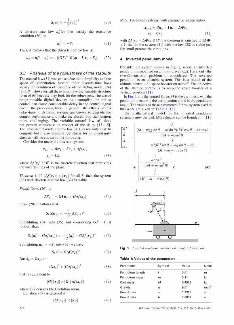
Consider the system shown in Fig. 1, where an invertedpendulum is mounted on a motor driven cart. Here, only thetwo-dimensional problem is considered. The invertedpendulum is an unstable system. This is a model of theattitude control of a space booster on takeoff. The objectiveof the attitude control is to keep the space booster in avertical position [11].

In Fig. 1 u is the control force, M is the cart mass, m is thependulum mass, x is the cart position and y is the pendulumangle. The values of these parameters for the system used inthis work are given in Table 1 [16].

The mathematical model for the inverted pendulumsystem is now derived. More details can be founded in [11].

_yy€yy

_xx

€xx

26664

37775 ¼

_yyðM þ mÞg sin y� mðsin yÞð_yyÞ2 cos yþ b_xx cos y

lðM þ m sin2 yÞ_xx

mlð_yyÞ2 sin y� mg sin y� b_xx

ðM þ m � m cos yÞ

266666664

377777775

þ

0

� a cos ylðM þ m sin2 yÞ

0a

ðM þ m � m cos yÞ

26666664

37777775

Vv ð42Þ

Fig. 1 Inverted pendulum mounted on a motor driven cart

Table 1: Values of the parameters

Parameter Symbol Value Units

Pendulum length l 0.61 m

Pendulum mass m 0.21 kg

Cart mass M 0.4573 kg

Gravity g 9.81 m=s2

Board data a 1.7378 –

Board data b 7.6832 –

IEE Proc.-Control Theory Appl., Vol. 152, No. 2, March 2005222

where the relation between the control force u and thetension Vv; in volts, from the power amplifier is [16]:

u ¼ aVv � b_xx ð43Þand the numeric values of a and b are given in Table 1.

After linearising the system near to ½y _yy x _xx ¼ ½0 0 0 0 ;we get:

_yy€yy

_xx

€xx

26664

37775 ¼

0 1 0 0ðMþmÞ

Mlg 0 0 b

Ml

0 0 0 1�mM

g 0 0 �bM

26664

37775

y_yy

x

_xx

26664

37775þ

0

� aMl

0aM

26664

37775Vv ð44Þ

5 Inverted pendulum system with SMC

This Section presents a design for a sliding mode controllerapplied to the inverted pendulum system.

It is assumed that all states are available for feedback.Equations (2) and (18) are used to compute the switchingsurface for the continuous and discrete controllers,respectively.

Using the plant (44), the values of the parameters fromTable 1 and (5) and (21), the switching surface has beencomputed for the continuous and discrete cases. Thiscomputation uses the pole-placement method for the systemin sliding mode.

The control law has been computed using (16) and (32)for the continuous and discrete cases, respectively.

The numeric values obtained for the continuous pendu-lum system (44), using the values of parameters fromTable 1, are given as follows:

A ¼

0 1:0 0 0

46:9 0 0 55:1

0 0 0 1:0

�4:5 0 0 �16:8

266664

377775 B ¼

0

�12:4

0

3:8

266664

377775

C ¼

1 0 0 0

0 1 0 0

0 0 1 0

0 0 0 1

266664

377775

ð45Þ

the discrete transformed system (17) for each sampletime can be easily obtained using the Matlab programfunction c2d.

The allocation poles technique was used to complete thesliding gains. The choice of the poles takes into account thesaturation of the used interface board A=D� D=A con-verters (5 V). Thus, the poles were chosen to be 210, 25and 23, which establish the reduced-order dynamics for thesystem in sliding mode, (5). The obtained constant values(9) for the continuous controller are:

G ¼ �348:1 �62:1 �466:2 �178:7½ ð46Þand

Feq ¼ 22:2 3:6 0 9:3½ :

The continuous control (15) was modified as follows:

u�n ðtÞ ¼ r

SðtÞkSðtÞk þ D

r< 0 ð47Þ

with r ¼ �1 and D ¼ 0:005: This modification was made toreduce the chattering effect [17].

For the discrete controller, the gains vary according tothe sample time and are obtained from (20) and (21).The corresponding obtained constant gains for a sampletime of 0.01 s are:

Feq ¼ ½ 11:6 1:9 0 5:6

G ¼ ½�180:5 �31:5 �121:8 �77:1 and for a sample time of 0.001 s the constant gains are:

Feq ¼ ½ 11:4 1:8 0 5:6

G ¼ ½�1817:9 �317:1 �1226:5 �776:8 The control used for the discrete case was u�

k ¼ �Sk;i.e. (31).

6 Simulations and experimental results

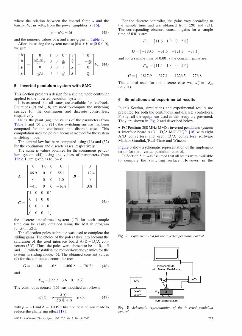
In this Section, simulations and experimental results arepresented for both the continuous and discrete controllers.Firstly, all the equipment used in this study are presented.They are shown in Fig. 2 and described below.

. PC Pentium 200 MHz MMX; inverted pendulum system;

. Interface board A=D� D=A MULTIQe [16] with eightA=D converters and eight D=A converters softwareMatlab=Simulink=Real-Time and Wincon.

Figure 3 show a schematic representation of the implemen-tation for the inverted pendulum control.

In Section 5, it was assumed that all states were availableto compute the switching surface. However, in the

Fig. 2 Equipment used for the inverted pendulum control

Fig. 3 Schematic representation of the inverted pendulumcontrol

IEE Proc.-Control Theory Appl., Vol. 152, No. 2, March 2005 223

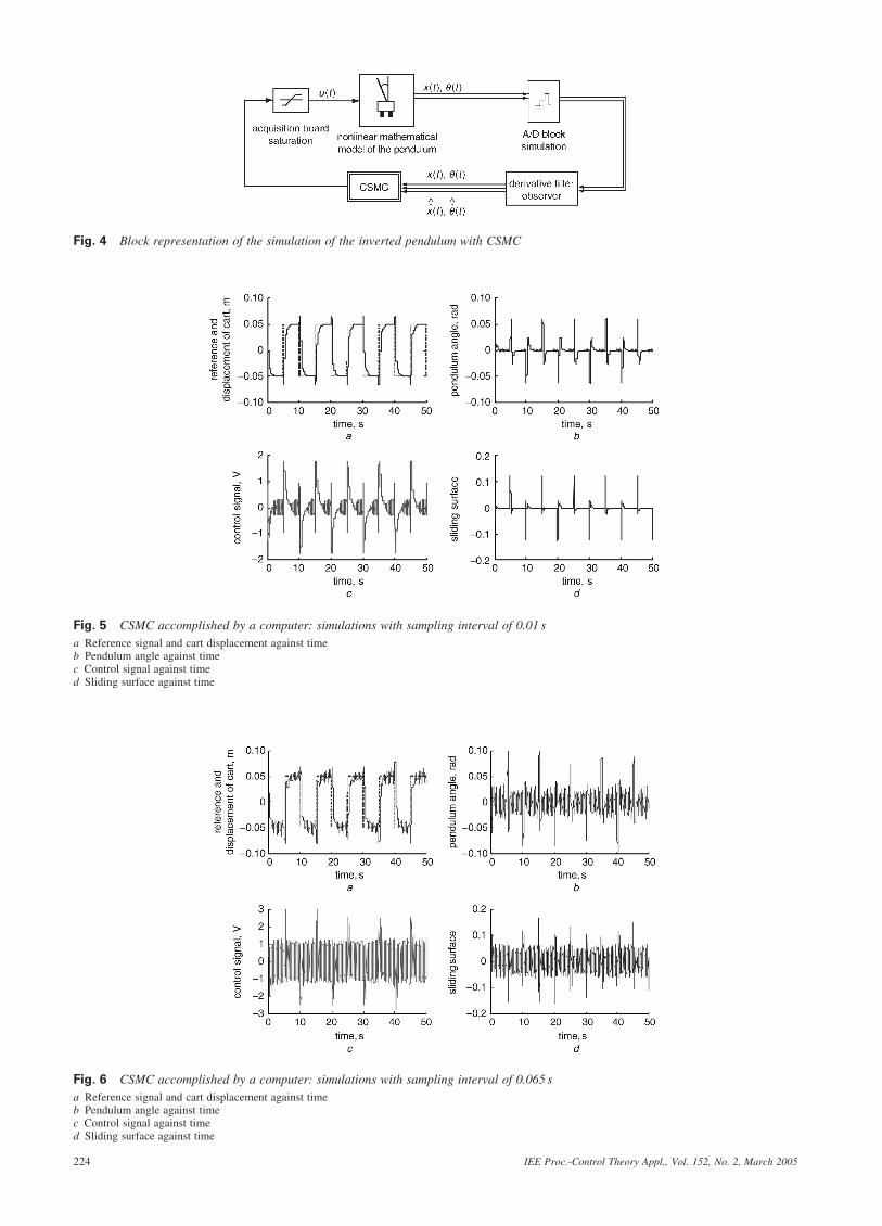
Fig. 4 Block representation of the simulation of the inverted pendulum with CSMC

Fig. 5 CSMC accomplished by a computer: simulations with sampling interval of 0.01 s

a Reference signal and cart displacement against timeb Pendulum angle against timec Control signal against timed Sliding surface against time

Fig. 6 CSMC accomplished by a computer: simulations with sampling interval of 0.065 s

a Reference signal and cart displacement against timeb Pendulum angle against timec Control signal against timed Sliding surface against time

IEE Proc.-Control Theory Appl., Vol. 152, No. 2, March 2005224

investigated inverted pendulum system, only two states,y and x, were available. To calculate the others states,_yy and _xx; we used a derivative filter created using theMatlab=Simulink=Real-Time software [16].

6.1 CSMC

6.1.1 Simulations: In Fig. 4 we show a blockrepresentation for the simulation of the inverted pendulumwith the CSMC (47). The results considering a square waveas reference signal and initial conditions ½y _yy x _xx ¼½0 0 0 0 are given in Figs. 5 and 6. The simulations takeinto account that the control is accomplished using acomputer. The sampling interval was not considered in thecontroller designs, but it was considered in the simulationsby the block ‘zero-order’ of the Simulink program. Thenonlinear model (42) was used for the simulation of thependulum system. Two cases are shown: sampling intervalsof 0.01 and 0.065 s. The results indicate that the systemperformance was deteriorated as the sampling periodincreases.

6.1.2 Experimental implementation: A con-tinuous controller (47) has been created using the softwareSimulink and Wincon as shown in Fig. 7. Some exper-imental results are shown in Fig. 8 and Fig. 9.

By the analysis of the simulation and experimental resultsit is observed that the continuous sliding mode control is

very sensitive to the sampling interval. The results indicatethat the system performance was deteriorated as thesampling period increases (Fig. 6 and Fig. 9).

6.2 DSMC

6.2.1 Simulations: The system with the proposeddiscrete sliding mode control (32) is shown, in Fig. 10. In thesimulations it was considered that the control law isachieved using a computer. The sampling interval wastaken into account in the design of the controller. Tosimulate the sampling interval we used the block ‘zero-order’ of the Simulink program.

Results of the simulation with a square wave as areference signal and initial conditions ½y _yy x _xx ¼ ½0 0 0 0 are shown in Figs. 11 and 12. Two cases are shown: asampling interval of 0.01 s (Fig. 11) and a sampling intervalof 0.1 s (Fig. 12). The results show a good performance ofthe system for both cases.

6.2.2 Experimental implementation: The pro-posed discrete controller (32) has been created using theSimulink and Wincon software as shown in Fig. 13. Twoexperimental results are shown in Figs. 14 and 15a:sampling interval of 0.001 s (Fig. 14) and a samplinginterval of 0.01 s (Fig. 15). The results indicate a goodperformance of the system for both cases.

Fig. 7 Continuous sliding mode controller accomplished using a computer

Fig. 8 CSMC accomplished using a computer: experimental results with a sampling interval of 0.001 s

a Displacement of the cart against timeb Pendulum angle against time

IEE Proc.-Control Theory Appl., Vol. 152, No. 2, March 2005 225

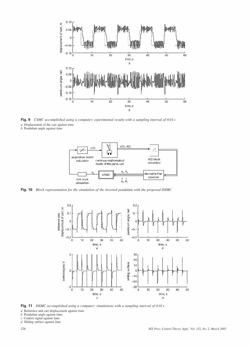
Fig. 9 CSMC accomplished using a computer: experimental results with a sampling interval of 0.01 s

a Displacement of the cart against timeb Pendulum angle against time

Fig. 10 Block representation for the simulation of the inverted pendulum with the proposed DSMC

Fig. 11 DSMC accomplished using a computer: simulations with a sampling interval of 0.01 s

a Reference and cart displacement against timeb Pendulum angle against timec Control signal against timed Sliding surface against time

IEE Proc.-Control Theory Appl., Vol. 152, No. 2, March 2005226

Fig. 12 DSMC accomplished using a computer: simulations with sampling interval of 0.1 s

a Reference signal and cart displacement against timeb Pendulum angle against timec Control signal against timed Sliding surface against time

Fig. 13 Discrete sliding mode controller accomplished using a computer

Fig. 14 DSMC accomplished using a computer: experimental results with sample time of 0.001 s

a Cart displacement as a function of timeb Pendulum angle as a function of time

IEE Proc.-Control Theory Appl., Vol. 152, No. 2, March 2005 227

7 Conclusions

In this work a computer-based SMC was analysed. Bothcontinuous-time and discrete-time SMC design was con-sidered. The continuous-time control design does not takeinto account the sampling period. Thus, just for very smallsampling periods the control system will have a goodperformance.

A new discrete sliding mode controller was proposed.This control design proposes a smooth sliding law, whichtakes in consideration the converters and the samplingperiod. The advantage of the proposed discrete law is thathis computation is very simple, once it doesn’t possessvariable structure. Thus, the computation of the proposedlaw is very fast, so that it avoids delay-time in the controldue to the computation. Also, it was proven that theproposed discrete control is robust for a certain uncertaintyclass.

Experiments on an inverted pendulum system werepresented. Simulations and experimental results for bothcontinuous-time and proposed discrete-time SMC designwas shown. The obtained results proved the effectiveness ofthe discrete-time SMC design, once the proposed discretecontroller has a good performance, even for larger values ofsampling periods and uncertainties.

8 Acknowledgment

The authors gratefully acknowledge the financial support byFAPESP.

9 References

1 Utkin, V.I.: ‘Sliding modes and their applications in variable structuresystems’ (Mir, Moscow, 1978)

2 Guo, J., and Zhang, X.: ‘Advance in discrete-time sliding modevariable structure control theory’. Proc. 4th World Congress onIntelligent Control and Automation, Shanghai, PRC, 2002, Vol. 2,pp. 878–882

3 Su, W.C., and Tsai, C.C.: ‘Discrete-time VSS temperature control fora plastic extrusion process with water cooling systems’, IEEE Trans.Control Syst. Technol., 2001, 9, (4), pp. 618–623

4 Zhou, J., Zhou, R., Wang, Y., and Guo, G.: ‘Improved proximate time-optimal sliding-mode control of hard disk drives’, IEE Proc., ControlTheory Appl., 2001, 148, (6), pp. 516–522

5 Li, Y.F., and Wikander, J.: ‘Discrete-time sliding mode control forlinear system with nonlinear friction’. Proc. 6th IEEE Int. Workshop onVariable structure systems, Gold Coast, Australia, 2000, pp. 35–44

6 Silva, S.G., Garcia, J.P.F., and Teixeira, M.C.M.: ‘Variable structurecontroller and observer applied to induction machine’. Proc. 5th Int.Workshop on Advanced Motion Control (AMC), 1998, Coimbra,Portugal, pp. 123–128

7 Decarlo, R.A., Zak, S.H., and Mathews, G.P.: ‘Variable structurecontrol of multivariable systems: A Tutorial’, Proc. IEEE ElectronicsEngineers, 1988, 76, pp. 212–232

8 Furuta, K.: ‘Sliding mode control of a discrete system’, Syst. ControlLett., 1990, 14, pp. 145–152

9 Chan, C.Y.: ‘Servo-systems with discrete variable structure control’,Syst. Control Lett., 1991, 17, pp. 321–325

10 Bandyopadhyay, B., and Saaj, C.M.: ‘Algorithm on robust sliding modecontrol for discrete-time system using fast output sampling feedback’,IEE Proc., Control Theory Appl., 2002, 149, (6), pp. 497–503

11 Ogata, K.: ‘Modern control engineering’ (Prentice-Hall, 1997, 3rd edn.)12 Fillipov, A.F.: ‘Differential equations with discontinuous righthand

sides’ (Kluwer Academic Publishers, 1988)13 Garcia, L.M.C., and Bennaton, J.F.: ‘Sliding mode control for uncertain

input-delay systems with only plant output acces’. Presented atAdvances in Variable Structure Systems – Theory and Applications,Philadelphia, PA, Sarajero, Bosnia and Herzegovina, July 2002

14 Hsu, K.J., Basker, V.R., and Crisalle, O.D.: ‘Sliding mode control ofuncertain input-delay systems’. Proc. American Control Conf.,Philadelphia, PA, June 1998, pp. 564–568

15 Choi, H.H., and Chung, M.J.: ‘Memoryless stabilization of uncertaindynamic systems with time varying delayed states and controls’,Automatica, 1995, 31, pp. 1349–1351

16 ‘Wincon v3. 0 – user’s guide’ (Quanser Consulting Inc., Ontario,Canada, 1998)

17 Spurgeon, S.K., and Davies, R.: ‘A nonlinear control strategy for robustsliding mode performance in the presence of unmatched uncertainty’,Int. J. Control, 1993, 57, (5), pp. 1107–1123

Fig. 15 DSMC accomplished using a computer: experimental results with sample time of 0.01 s

a Cart displacement as a function of timeb Pendulum angle as a function of time

IEE Proc.-Control Theory Appl., Vol. 152, No. 2, March 2005228