APPENDIX C.6 Normal Distributions A43

Continuous Random Variables

As discussed in Appendix C.5, a random variable associated with an experimentthat has a finite number of possible outcomes is called a discrete random vari-able. For example, if a coin is tossed three times and a random variable isassigned that counts the number of heads that turn up, then there are only fourvalues the random variable can have 0, 1, 2, or 3. (see Figure C.25.)

FIGURE C.25

In this appendix you will study experiments for which there are an infinitenumber of possible outcomes. For example, consider an experiment that measures the actual number of ounces of toothpaste in a tube that is labeled “10 ounces.” The actual weight could be 10.02 ounces, or 10.024 ounces, or10.0247 ounces, and so on. There are infinitely many different possible weights.Suppose that the possible weights vary between 9.5 ounces and 10.5 ounces. Therange of the random variable needed for this experiment would be

Range of random variable

This type of random variable is a continuous random variable because it canhave any value in the interval between 9.5 ounces and 10.5 ounces. (See FigureC.26.)

FIGURE C.26

Because there are an infinite number of values in the interval between 9.5 and10.5, you cannot list each possible value of the random variable and assign prob-abilities to those values (as you did for a discrete random variable). To measureprobabilities for a continuous random variable, you must use a method thatinvolves measuring the area of a region under a graph.

x

10.59.5

10

9.5 ≤ x ≤ 10.5.

x

0 1 2 3

C.6 Normal Distributions■ Find probabilities for continuous random variables.

■ Find probabilities using the normal distribution.

■ Find probabilities using the standard normal distribution.

■ Find probabilities using z-scores for nonstandard normal distributions.

A function that is used to measure probabilities for a continuous randomvariable is called a probability density function. Three common types of probability density functions are uniform, exponential, and normal probabilitydensity functions, as shown in Figure C.27.

FIGURE C.27

For each of the probability density functions shown in Figure C.27, the rangeof the continuous random variable is an interval on the real line. For the uniformprobability density function, the range is the closed interval which impliesthat the random variable can take on any value between and (including or). For the exponential probability density function, the range is the interval

which implies that the random variable can take on any nonnegativevalue. For the normal probability density function, the range is the interval

which implies that the random variable can take on any value.As indicated in Figure C.27, the area of the region that lies between the graph

of a probability density function and the -axis is 1. This corresponds to the factthat, for a discrete random variable, the sum of all probabilities must be 1.

x

���, ��,

�0, ��,b

abax�a, b�,

x

f(x)

Area = 1

1b − a

a b

Uniform ProbabilityDensity Function

Exponential ProbabilityDensity Function

x

f(x)

Area = 1

Normal ProbabilityDensity Function

x

f(x)

Area = 1

A44 APPENDIX C Probability and Probability Distributions

Example 1 Uniform Probability Density Function

The flight time for a trip from Atlanta to Pittsburgh on a certain airline has beenfound to vary between 2.5 hours (150 minutes) and 3.5 hours (210 minutes).Moreover, the probability of the flight time falling in any given one-minute inter-val in this range is the same. That is, the model used to represent the probabilitiesis the uniform probability density function

(See Figure C.28.) Find the probability that the flight time for a flight is between170 minutes and 180 minutes.

SOLUTION From Figure C.28, note that the area of the region under the graph ofthe uniform probability density function is 1. You can verify this by using the formula for the area of a rectangle:

To find the probability that the flight time is between 170 and 180 minutes, findthe area of a smaller rectangle whose width is the interval That is,

✓CHECKPOINT 1

In Example 1, what is the probability that a flight will take more than 3 hours? ■

All uniform probability density functions have the form

Uniform probability density function

As shown in Figure C.29, the width of the rectangular region corresponding to auniform probability density function is and the height is So,the area is

FIGURE C.29

x

f(x)

1 b − a

1 b − a

a b c d

Uniform Probability Density Function

P(c ≤ x ≤ d) = (d − c)( (

P�a ≤ x ≤ b� � �b � a�� 1b � a� � 1.

1��b � a�.�b � a�

a ≤ x ≤ b. f�x� �1

b � a,

P�170 ≤ x ≤ 180� � �width� � �height� � �180 � 170� � � 160� 0.167.

�170, 180�.

P�150 ≤ x ≤ 210� � �width� � �height� � �210 � 150� � � 160� � 1.

150 ≤ x ≤ 210. f�x� �160

,

APPENDIX C.6 Normal Distributions A45

Flight time (in minutes)

Uniform ProbabilityDensity Function

Prob

abili

ty

x150

f(x)

160

160

160 170 180 190 200 210

Height =

Width = 10

FIGURE C.28

So, for a uniform probability density function, the probability that lies in theinterval (where ) is

The expected value (or mean) of a uniform probability density function isthe midpoint of the interval Try showing that

and

From this discussion about uniform probability density functions, you shouldobserve the following important facts, which apply to all probability densityfunctions.

1. With a probability density function, the probability that the random variablewill have an exact value is insignificant. So, the probability that the value ofthe random variable lies in a particular interval is found.

2. The area of the region under the graph of a probability density function is 1.

3. The probability that a continuous random variable will lie in an interval isdefined to be the area of the region between the interval on the -axis and thegraph of the probability density function.

Normal Distribution

In practice, the most widely used probability density function is the normalprobability density function. This function can be applied to many practicalproblems that occur in the life and social sciences. The equation that is used torepresent a normal probability density function is

Normal probability density function

You will see, however, that it is usually not necessary to use this equation to solveproblems involving normal distributions.

The graph of a normal probability density function is called the normalcurve, and the associated probability distribution is called the normal distribu-tion. A normal curve is “bell-shaped,” as shown in Figure C.30. Note that thecurve is symmetric about the mean The percentages shown in this figure arevalid for all normal distributions. For example, for all normal distributions, theprobability that an outcome will fall between and is 0.341.

Also, approximately 95% of the total region under a normal curve lies with-in two standard deviations of the mean.

� � ��

�.

f�x� �1

�2 e��x ���2�2� 2

x

P�a � b2

≤ x ≤ b� �12

.P�a ≤ x ≤a � b

2 � �12

�a, b�.�a � b��2,

P�c ≤ x ≤ d� � �d � c�� 1b � a�.

a ≤ c ≤ d ≤ bc ≤ x ≤ dx

A46 APPENDIX C Probability and Probability Distributions

μ+μ

σ2+μσ−μ

σ+μ

σ3−μσ3 −μ

σ2

x

f(x)

Approximately 68% of data items

Approximately 95% of data items

Nearly all data items (99.74%)

34.1%

13.6%

2.2%

FIGURE C.30

S T U D Y T I PFor a more detailed discussion of expected value and standard deviation of acontinuous random variable, see Section 11.3.

Example 2 Normal Distribution

The lifetimes of tires are normally distributed with a mean of 50,000 miles and a standard deviation of 2500 miles. Use Figure C.30 to answer the followingquestions.

a. What is the probability that a tire will last for 50,000 miles or more?

b. What is the probability that a tire will last for 52,500 miles or less?

c. What is the probability that a tire will last between 47,500 miles and 55,000miles?

SOLUTION Using the probabilities shown in Figure C.30, you can obtain thegraph and probabilities shown in Figure C.31.

a. Because the distribution is normal, half of the area under the curve lies to theright of the mean. So, the probability that a tire will last for 50,000 or moremiles is

b. Because half of the tires will last for 50,000 miles or less, and 34.1% will lastbetween 50,000 miles and 52,500 miles, the probability that a tire will last for52,500 miles or less is approximately

or approximately 84.1%.

c. Using Figure C.31, the probability that a tire will last between 47,500 milesand 55,000 miles is approximately

or approximately 81.8%.

✓CHECKPOINT 2

A medical researcher has determined that for a group of 100 women, thelengths of pregnancies from conception to birth are normally distributed with a mean of 266 days and a standard deviation of 12 days.

a. What is the probability that a pregnancy will last for 266 days or more?

b. What is the probability that a pregnancy will last for 278 days or less?

c. What is the probability that a pregnancy will last between 266 and 278 days? ■

P�47,500 ≤ x ≤ 55,000� � 0.341 � 0.341 � 0.136 � 0.818

P�x ≤ 52,500� � 0.500 � 0.341 � 0.841

P�x ≥ 50,000� �12

� 0.500.

APPENDIX C.6 Normal Distributions A47

x

f(x)

34.1%34.1%

42,500 47,500 52,500 57,500

Prob

abili

ty

Tire lifetime (in miles)

13.6% 13.6%

2.2% 2.2%

Tire Lifetime

FIGURE C.31

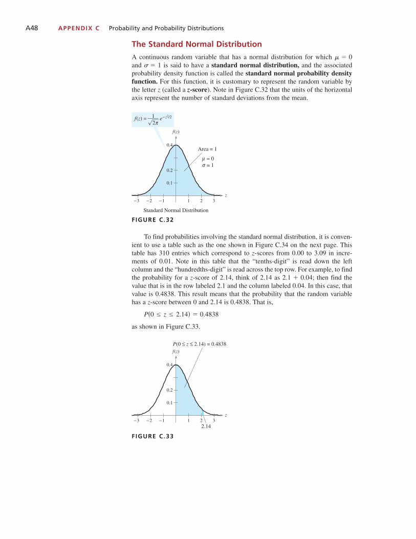
The Standard Normal Distribution

A continuous random variable that has a normal distribution for which and is said to have a standard normal distribution, and the associated probability density function is called the standard normal probability densityfunction. For this function, it is customary to represent the random variable bythe letter (called a z-score). Note in Figure C.32 that the units of the horizontalaxis represent the number of standard deviations from the mean.

FIGURE C.32

To find probabilities involving the standard normal distribution, it is conven-ient to use a table such as the one shown in Figure C.34 on the next page. Thistable has 310 entries which correspond to -scores from 0.00 to 3.09 in incre-ments of 0.01. Note in this table that the “tenths-digit” is read down the left column and the “hundredths-digit” is read across the top row. For example, to findthe probability for a -score of 2.14, think of 2.14 as then find thevalue that is in the row labeled 2.1 and the column labeled 0.04. In this case, thatvalue is 0.4838. This result means that the probability that the random variablehas a -score between 0 and 2.14 is 0.4838. That is,

as shown in Figure C.33.

FIGURE C.33

z

f(z)

−1−2−3 1 22.14

3

0.1

0.2

0.4

P(0 ≤ z ≤ 2.14) = 0.4838

P�0 ≤ z ≤ 2.14� � 0.4838

z

2.1 � 0.04;z

z

z

f(z)

−1 −2 −3 1 2 3

0.1

0.2

0.4

Standard Normal Distribution

f(z) = e−z2/2

2 π 1

Area = 1

= 0= 1

μ σ

z

� � 1� � 0

A48 APPENDIX C Probability and Probability Distributions

FIGURE C.34 Standard Normal Table (z-Scores)

zz-score

f(z)

0.0 .0000 .0040 .0080 .0120 .0160 .0199 .0239 .0279 .0319 .03590.1 .0398 .0438 .0478 .0517 .0557 .0596 .0636 .0675 .0714 .07530.2 .0793 .0832 .0871 .0910 .0948 .0987 .1026 .1064 .1103 .11410.3 .1179 .1217 .1255 .1293 .1331 .1368 .1406 .1443 .1480 .15170.4 .1554 .1591 .1628 .1664 .1700 .1736 .1772 .1808 .1844 .18790.5 .1915 .1950 .1985 .2019 .2054 .2088 .2123 .2157 .2190 .2224

0.6 .2257 .2291 .2324 .2357 .2389 .2422 .2454 .2486 .2517 .25490.7 .2580 .2611 .2642 .2673 .2704 .2734 .2764 .2794 .2823 .28520.8 .2881 .2910 .2939 .2967 .2995 .3023 .3051 .3078 .3106 .31330.9 .3159 .3186 .3212 .3238 .3264 .3289 .3315 .3340 .3365 .33891.0 .3413 .3438 .3461 .3485 .3508 .3531 .3554 .3577 .3599 .3621

1.1 .3643 .3665 .3686 .3708 .3729 .3749 .3770 .3790 .3810 .38301.2 .3849 .3869 .3888 .3907 .3925 .3944 .3962 .3980 .3997 .40151.3 .4032 .4049 .4066 .4082 .4099 .4115 .4131 .4147 .4162 .41771.4 .4192 .4207 .4222 .4236 .4251 .4265 .4279 .4292 .4306 .43191.5 .4332 .4345 .4357 .4370 .4382 .4394 .4406 .4418 .4429 .4441

1.6 .4452 .4463 .4474 .4484 .4495 .4505 .4515 .4525 .4535 .45451.7 .4554 .4564 .4573 .4582 .4591 .4599 .4608 .4616 .4625 .46331.8 .4641 .4649 .4656 .4664 .4671 .4678 .4686 .4693 .4699 .47061.9 .4713 .4719 .4726 .4732 .4738 .4744 .4750 .4756 .4761 .47672.0 .4772 .4778 .4783 .4788 .4793 .4798 .4803 .4808 .4812 .4817

2.1 .4821 .4826 .4830 .4834 .4838 .4842 .4846 .4850 .4854 .48572.2 .4861 .4864 .4868 .4871 .4875 .4878 .4881 .4884 .4887 .48902.3 .4893 .4896 .4898 .4901 .4904 .4906 .4909 .4911 .4913 .49162.4 .4918 .4920 .4922 .4925 .4927 .4929 .4931 .4932 .4934 .49362.5 .4938 .4940 .4941 .4943 .4945 .4946 .4948 .4949 .4951 .4952

2.6 .4953 .4955 .4956 .4957 .4959 .4960 .4961 .4962 .4963 .49642.7 .4965 .4966 .4967 .4968 .4969 .4970 .4971 .4972 .4973 .49742.8 .4974 .4975 .4976 .4977 .4977 .4978 .4979 .4979 .4980 .49812.9 .4981 .4982 .4982 .4983 .4984 .4984 .4985 .4985 .4986 .49863.0 .4987 .4987 .4987 .4988 .4988 .4989 .4989 .4989 .4990 .4990

z .00 .01 .02 .03 .04 .05 .06 .07 .08 .09

Hundredths Digit for z-score

Tent

hs D

igit

for

z-sc

ore

APPENDIX C.6 Normal Distributions A49

Example 3 Using the Standard Normal Tables

Use Figure C.34 to determine the following probabilities.

a. b.

c. d.

SOLUTION

a. To determine find the value that is in the row labeled 1.0 andthe column labeled .02. That value is 0.3461. So,

b. To determine first use the symmetry of the standard normal probability density function to conclude that

Then, using the row labeled 1.4 and the column labeled .03,you can conclude that

c. To determine use the fact that

From Figure C.34, and So,

d. To determine use the fact that

Because and you can con-clude that

The areas corresponding to these four probabilities are shown in Figure C.35.

✓CHECKPOINT 3

Use Figure C.34 to determine the following probabilities.

a. b.

c. d. ■P�z ≥ 0.37�P�0.55 ≤ z ≤ 1.06�

P��2.14 ≤ z ≤ 0�P�0 ≤ z ≤ 0.98�

P�z ≥ 0.76� � 1 � 0.5000 � 0.2764 � 0.2236.

P�0 ≤ z ≤ 0.76� � 0.2764,P�z ≤ 0� � 0.5000

P�z ≤ 0� � P�0 ≤ z ≤ 0.76� � P�z ≥ 0.76� � 1.

P�z ≥ 0.76�,

P�0.14 ≤ z ≤ 1.23� � 0.3907 � 0.0557 � 0.3350.

P�0 ≤ z ≤ 0.14� � 0.0557.P�0 ≤ z ≤ 1.23� � 0.3907

P�0.14 ≤ z ≤ 1.23� � P�0 ≤ z ≤ 1.23� � P�0 ≤ z ≤ 0.14�.

P�0.14 ≤ z ≤ 1.23�,

P��1.43 ≤ z ≤ 0� � P�0 ≤ z ≤ 1.43� � 0.4236.

P�0 ≤ z ≤ 1.43�.P��1.43 ≤ z ≤ 0� �

P��1.43 ≤ z ≤ 0�,

P�0 ≤ z ≤ 1.02� � 0.3461

P�0 ≤ z ≤ 1.02�,

P�z ≥ 0.76�P�0.14 ≤ z ≤ 1.23�

P��1.43 ≤ z ≤ 0�P�0 ≤ z ≤ 1.02�

A50 APPENDIX C Probability and Probability Distributions

z−1−2−3 1 2 3

P(0 ≤ z ≤ 1.02)

(a)

z−1−2−3 1 2 3

P(−1.43 ≤ z ≤ 0)

(b)

z−1−2−3 1 2 3

P(0.14 ≤ z ≤ 1.23)

z−1−2−3 1 2 3

P(z ≥ 0.76)

(c)

(d)

FIGURE C.35

APPENDIX C.6 Normal Distributions A51

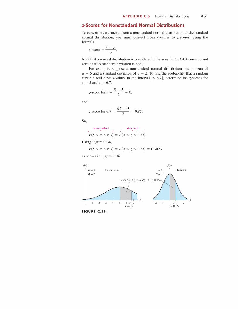
z-Scores for Nonstandard Normal Distributions

To convert measurments from a nonstandard normal distribution to the standardnormal distribution, you must convert from -values to -scores, using the formula

Note that a normal distribution is considered to be nonstandard if its mean is notzero or if its standard deviation is not 1.

For example, suppose a nonstandard normal distribution has a mean ofand a standard deviation of To find the probability that a random

variable will have -values in the interval determine the -scores forand

and

So,

nonstandard standard

Using Figure C.34,

as shown in Figure C.36.

FIGURE C.36

zx

P(5 ≤ x ≤ 6.7) = P(0 ≤ z ≤ 0.85)

Nonstandard Standard

x = 6.71 2 3 4 5 6 7 −1−2 1 2

f(z)f(x)

z = 0.85

= 5= 2

μσ

= 0= 1

μσ

P�5 ≤ x ≤ 6.7� � P�0 ≤ z ≤ 0.85� � 0.3023

P�5 ≤ x ≤ 6.7� � P�0 ≤ z ≤ 0.85�.

z-score for 6.7 �6.7 � 5

2� 0.85.

z-score for 5 �5 � 5

2� 0.

x � 6.7:x � 5z�5, 6.7�,x

� � 2.� � 5

z-score �x � �

�.

zx

Example 4 Finding Probabilities for Nonstandard Distributions

The mean speed of traffic (as checked by radar) on a stretch of interstate highwayis 68 miles per hour with a standard deviation of 4 miles per hour. Assuming thatthe speeds of vehicles on this section of highway are normally distributed, deter-mine what percentage of the vehicles are exceeding the legal speed of 65 milesper hour.

SOLUTION Because the mean is 68 and the standard deviation is 4, the -scorefor 65 miles per hour is

Using Figure C.34, the percentage of vehicles is approximately

✓CHECKPOINT 4

In Example 4, what percentage of vehicles are traveling between 65 and 70 miles per hour? ■

� 77.34%.

� 0.7734

� 0.2734 � 0.5000

� P�0 ≤ z ≤ 0.75� � P�z ≥ 0� P�x > 65� � P�z ≥ �0.75� � P��0.75 ≤ z ≤ 0� � P�z ≥ 0�

z �65 � 68

4� �0.75.

z

A52 APPENDIX C Probability and Probability Distributions

1. A ______ random variable can take on any value in a given interval.

2. What is the total area of the region under the graph of a probability density function?

3. In the normal probability density function

which variable represents the mean? Which variable represents the standard deviation?

4. A continuous random variable that has a normal distribution for whichand is said to have the ______ normal distribution.� � 1� � 0

f �x� �1

�2e��x � ��2�2� 2,

C O N C E P T C H E C K

APPENDIX C.6 Normal Distributions A53

In Exercises 1–4, find the indicated probabilities forthe given uniform probability density function.

1.

(a) (b)

(c) (d)

2.

(a) (b)

(c) (d)

3.

(a) (b)

(c) (d)

4.

(a) (b)

(c) (d)

5. Departure Time Buses arrive and depart from a collegeevery 20 minutes. The probability density function for thewaiting times (in minutes) for people arriving at random is

Find the probability that a person will wait (a) no more thanfive minutes, and (b) at least 12 minutes.

6. Flight Time The flight times for trips from Miami toAtlanta on an airline has been found to vary between 90minutes and 160 minutes. The probability density functionfor the flight times (in minutes) is

Find the probability that a flight will take (a) between 100and 110 minutes, and (b) more than 2 hours.

In Exercises 7–16, use the standard normal table inFigure C.34 to find the indicated probability.

7. 8.

9. 10.

11. 12.

13. 14.

15. 16. P�z ≥ 1.5�P�z ≥ �0.52�P�z ≤ 2.71�P�z ≤ 1.93�P��2.42 ≤ z ≤ �1.12�P��1.5 ≤ z ≤ �0.07�P�0.34 ≤ z ≤ 0.96�P��1.01 ≤ z ≤ 0�P�0 ≤ z ≤ 2.05�P�0 ≤ z ≤ 0.93�

90 ≤ x ≤ 160. f �t� �1

70,

t

0 ≤ t ≤ 20. f �t� �1

20,

t

P�x ≤ 75�P�x ≥ 75�P�x ≥ 100�P�x ≤ 100�

75 ≤ x ≤ 100 f �x� �125,

P�x ≥ 95�P�110 ≤ x ≤ 130�P�110 ≤ x ≤ 125�P�112 ≤ x ≤ 120�

95 ≤ x ≤ 125 f �x� �130,

P�130 ≤ x ≤ 220�P�168 ≤ x ≤ 210�P�x ≥ 220�P�x ≤ 130�

130 ≤ x ≤ 220 f �x� �190,

P�x ≥ 80�P�50 ≤ x ≤ 75�P�50 ≤ x ≤ 60�P�x ≤ 70�

45 ≤ x ≤ 90 f �x� �145,

The following warm-up exercises involve skills that were covered in earlier sections. You will usethese skills in the exercise set for this section. For additional help, review Sections 11.1 and 11.2.

In Exercises 1 and 2, use the discrete probability distribution to determinethe indicated probabilities.

(a) (b)

(a) (b)

In Exercises 3–6, determine whether the function f represents a probabilitydensity function over the given interval. If f is not a probability density function, identify the conditions(s) that is (are) not satisfied.

3. 4.

5. 6. ��5, 5� f �x� � 0.006�25 � x2�,�0, �� f �x� �32e�3x�2,

�0, 10� f �x� �1

11,�1, 10� f �x� �19,

P�x ≥ 0�P��1 ≤ x ≤ 1�

P�x > 2�P�x ≤ 2�

Skills Review C.6

Exercises C.6 See www.CalcChat.com for worked-out solutions to odd-numbered exercises.

x 0 1 2 3 4

P�x� 216

316

616

316

216

x �2 �1 0 1 2

P�x� 0.078 0.234 0.376 0.234 0.078

1.

2.

In Exercises 17–24, find the indicated probability for acontinuous random variable x that is normally distrib-uted with a mean of 30 and standard deviation of 5.

17. 18.

19. 20.

21. 22.

23. 24.

In Exercises 25–32, find the indicated probability for acontinuous random variable x that is normally distrib-uted with a mean of 15 and a standard deviation of 3.

25. 26.

27. 28.

29. 30.

31. 32.

33. Monthly Utility Bill The monthly utility bills in a cityare normally distributed with a mean of $60 and a standarddeviation of $6. What is the probability that the utility billfor a household in the city, chosen at random, is (a)between $56 and $74, (b) less than $54, and (c) between$65 and $70?

34. Subscription Rates The weekly health magazine salesper sales-person for a publishing company are normallydistributed with a mean of 50 subscriptions and a standarddeviation of 4 subscriptions. In any one week, what is theprobability that a salesperson, chosen at random, will sell(a) between 39 and 45 subscriptions, (b) more than 47 sub-scriptions, and (c) more than 56 subscriptions?

35. Quality Control The lengths of hypodermic needlesproduced by a medical supply manufacturer are normallydistributed with a mean length of 1 inch and a standarddeviation of 0.02 inch. What is the probability that a needlewill have a length greater than 1.02 inches?

36. Quality Control One-liter bottles on an assembly lineare filled by a liquid-dispensing machine. The amounts ofliquid in the bottles are normally distributed with a mean of1 liter and a standard deviation of 0.1 liter. What is theprobability that the machine fills a bottle with less than0.95 liter?

37. Income Variation The annual incomes of associateprofessors at a college are normally distributed with a meanof $66,300 and a standard deviation of $5000. What is theprobability that an associate professor at the college has asalary higher than $70,000?

38. SAT Scores SAT math scores for a group of high schoolseniors are normally distributed with a mean of 500 and astandard deviation of 100. What percentage of the studentshave scores (a) below 400, (b) above 700, and (c) between500 and 600?

In Exercises 39–44, find the indicated probabilitiesusing the exponential probability density function.

Remember from Section 11.2 that the probability thatt lies in the interval is

39. If find

40. If find

41. If find

42. If find

43. Waiting Time The waiting times (in minutes) forpatients arriving at a doctor’s office are exponentially dis-tributed with Find the probability of waiting (a)less than 10 minutes, and (b) between 10 and 20 minutes.

44. Shelf Life The shelf lifes (in years) of a drug are exponentially distributed with A pharmacy has aquantity of this drug in stock and plans to replace the supply during regularly scheduled inventory replenishmentperiods. How much time should elapse between inventoryreplenishment periods if at least 95% of the supply is toremain within the shelf life throughout the period?

In Exercises 45–50, use a symbolic integration utility tofind the indicated probability for a random variable zthat has the standard normal distribution. Compareyour results to those given in the standard normaltable (Figure C.34).

45. 46.

47. 48.

49. 50.

51. Quality Control The lengths of flexible plastic cathetersproduced by a medical supply manufacturer are normallydistributed with a mean length of 4 inches and a standarddeviation of 0.07 inch. Use a symbolic integration utility todetermine the probability that a catheter will have a length(a) less than 3.9 inches, (b) greater than 4.1 inches, and (c)between 3.9 and 4.1 inches.

52. SAT Scores Nationally in 2006, the SAT math scoresroughly followed a normal distribution with a mean of 518and a standard deviation of 115. Using a symbolic integra-tion utility, find the percentage of students who had scores(a) below 400, (b) above 700, and (c) between 500 and 600.Compare your results to those of Exercise 38. Would yousay that the students’ scores in Exercise 38 were better orworse than the 2006 national scores? Explain. (Source:College Board)

P�z ≥ 1.0�P�0.3 ≤ z ≤ 2.0�P��1.5 ≤ z ≤ 0.3�P��1.5 ≤ z ≤ 2.0�P�z ≤ 2.0�P�0.0 ≤ z ≤ 2.0�

� 4.5.

� 16.

t

P�0.1 ≤ t ≤ 0.2�. � 0.06,

P�0.5 ≤ t ≤ 2�. �52,

P�0 ≤ t ≤ 1�. �13,

P�1 ≤ t ≤ 3�. � 3,

P�c } t } d � � d

cf �t�dt.

[c, d ]

[0, ��. f �t� �1

e�t�,

P�x ≥ 19�P�x ≥ 9�P�x ≤ 20�P�x ≤ 18�P�19 ≤ x ≤ 22�P�17 ≤ x ≤ 20�P�7 ≤ x ≤ 11�P�8 ≤ x ≤ 13�

P�21 ≤ x ≤ 45�P�19 ≤ x ≤ 36�P�25 ≤ x ≤ 35�P�20 ≤ x ≤ 40�P�18 ≤ x ≤ 30�P�23 ≤ x ≤ 30�P�30 ≤ x ≤ 37�P�30 ≤ x ≤ 35�

A54 APPENDIX C Probability and Probability Distributions