CONTINUOUS MONITORING OF AMBIENT VIBRATION … · 1 continuous monitoring of ambient vibration in...

1

CONTINUOUS MONITORING OF AMBIENT VIBRATION IN BUILDING: TIME AND SPACE STABILITY OF DYNAMIC

PARAMETERS FROM CGS BUILDING (ALGIERS, ALGERIA)

Bertrand GUILLIER1, Jean-Luc CHATELAIN2, Djamel MACHANE3, Mohamed FARSI4, Hugo PERFETTINI5, El Hadi OUBAICHE6, Rabah BENSALEM7 and Mustapha Hellel8

ABSTRACT

During a month, a continuous survey of ambient vibrations has been carried out on the Algerian National Center for Applied Research in Paraseismic Engineering (CGS) building, located in Algiers, Algeria. Providing data over ten synchronous sensors (five at the roof, four on the vertical of the building (more one on the roof) and one outside the building, on soil), it has been continuously monitored three different dynamic parameters of this building: the fundamental frequencies (in both directions of the building), their corresponding damping and their corresponding modal shape. This work underlines that both fundamental frequency and damping fluctuations (day-night variations) are linked one to another and not linked to the energy assessed in the building (or to the small strain generated by ambient vibrations) due to a too long delay between the frequency-damping maxima and the maxima of the energy assessed inside the building. However, it is strongly suspected a relationship between the temperature of the building materials and the frequency-damping temporal oscillations. This relationship is not straightforward as there is a delay between the external temperature maxima (or thermal insulation) and the frequency-damping maxima, temporal delay analyzed as a consequence of material properties of the building (thermal conductivity, specific heat capacity, thermal delay), leading to time-shift of the different maxima. The modal shape is steady over time. Moreover, it is shown that the place and the time of a single measurement can bias the determination of dynamic parameters of a building. Finally, it is compared two different procedures to calculate the building fundamental frequency from ambient vibrations, without significant difference, except that one of them give an evaluation of the frequency error, even for a single measurement.

INTRODUCTION As well as the frequency soil resonance, from an engineering point of view the elastic

fundamental (or modal) frequencies of structures are key-parameters to evaluate simplified seismic behavior of buildings (and so on their responses to earthquake shaking) and perhaps the more studied parameters due to the relative facility to determine it. To identify these fundamental frequencies, a lot of methods can be used as: unbinding, harmonic excitation or percussion, so generally dynamic

1 Dr, ISTerre, Grenoble, France, [email protected] 2 Dr, ISTerre, Grenoble, France, [email protected] 3 Dr, CGS, Algiers, Algeria, [email protected] 4 Dr, CGS, Algiers, Algeria, [email protected] 5 Dr, ISTerre, Grenoble, France, [email protected] 6 Dr, CGS, Algiers, Algeria, [email protected] 7 Dr, CGS, Algiers, Algeria, [email protected] 8 Dr, ISMAL, Algiers, Algeria, [email protected]

2

methods (Trifunac 1972; Luong et al 1992; Boutin et al 2001) that cannot be used for long to middle term surveys. In the same way, studies using earthquake records are very useful (Dunand et al. 2006; Guillier et al. 2007b), but the time of instrumentation waiting for an earthquake (especially in low to moderate seismic hazard regions) in the appropriate frequency range is problematic too. In the case of study on several days, the more used method is based on the use of ambient vibrations recorded in situ as done from a long time now (Crawford and Ward 1964; Trifunac 1972; Trifunac et al. 2001a, 2001b; Michel et al. 2010). The strong advantage of this ambient vibration method, used in this paper, is that the information needed is a priori presents everywhere in the building and at any time, when the main problem of this method is to derive structural behavior of the structure from weak-motion excitation (ambient vibration, 10-5<PGA<10-3 ms-2) to moderate to strong-motion (PGA>1 ms-2) as the building response is probably nonlinear in the higher energy shakes (strong-motion). Another important dynamic parameter is the damping of the previously defined modal frequencies (Jeary 1986; Satake et al. 2003) that can be extracted from ambient vibration using decrement methods (Vandiver et al. 1982; Ibrahim et al. 1998; Andersen et al. 2000; Dunand 2005). The damping is one of the most important dynamic parameters of a building as it deals with the propensity of a building to dissipate its internal energy. Finally, a third parameter, the modal shape, can be computed from ambient vibration (depending of the geometry of the array in the building). This parameter corresponds to evaluate how the energy is distributed vertically in the entire building, as the energy repartition should be normally increasing linearly from the foundations of the building (lower spectral energy) to its top (higher spectral energy). The study of building dynamic parameters has various interests as their evolution at mid to large-scaled time (ageing) or for post-seismic evaluation purposes (Guillier et al. 2007b; Farsi et al. 2009; Todorovska 2009).

As on soil dynamic parameters, a lot of authors have dealt with dynamic parameters of building (Trifunac 1972 to Michel et al. 2010), including the time evolution of these parameters in time (Herak and Herak 2010). In general, for a building, the main parameters presumed to control any changes in the modal frequencies, the damping and the modal shape can be divided in two types (i) permanent and strong changes, mainly due to modification in the structure (masonry [wall suppression…] or earthquake) and (ii) temporary changes that can be du to temporal external parameter mainly the level of energy exciting the building and also climatic conditions (water level, humidity…). The aim of this paper is to evaluate, from ambient vibration survey, the time behaviors of three building dynamic parameters as modal frequencies (in 2 orthogonal-horizontal directions), their corresponding damping coefficients and finally the modal shapes of the structure. These parameters fluctuations will be quantified and then analyzed to find possible explanations for these short-time changes.

1 Building, material-data collecting, and data processing

1.1 Building The studied building is located in the Hussein-Dey city, in the Algiers urban community in Algeria, in a moderate seismic area, at 800 meters South from the sea. This building is the main office of the Algerian National Center for Applied Research in Paraseismic Engineering (CGS). This building is 3.5 stairs high (10 meters high), as is base is overelevated of a half stair. Its size is 40x10 meters with a seismic joint in the middle of the structure, giving 2 (20x10) meters blocks placed side by side. This double-block building is made in reinforced concrete (RC) with masonry filling frame. Following the local way of living, in Algeria the weekend is set from 12-midnight on Wednesday to 12-midnight on Friday. 1.2 Material and data collecting For this experiment, it has been used 5 CitySharkII stations, (Chatelain et al 2000) from which 4 were connected to a 3C seismometer, when the last station was working with 6 3C seismometers giving a total of 10 seismometers, the 5 CitySharks stations had GPS time. The seismometers used were Lennartz LE-3D 5s, material and association of material compatible for microtremor studies (Guillier et al. 2007a). The seismometers have been installed in a common way: the North has been systematically oriented parallel to main length of the building (called longitudinal or long.) always in the same direction, so the East of the seismometer falls always parallel to the shorter length of the building (called transverse or trans.) and in the same direction (Fig. 1). Finally, when the seismometers were put outside (top of the roof or soil) and to keep the sensors away from any direct rain we

Guillier et al. 3

protected them by a plastic crate, enough ballasted to avoid any problem of wind, following the recommendations of Mucciarelli at al. (2005) and Chatelain et al. (2008) given for the use of ambient vibrations for H/V recordings. The array geometry of the seismometers is the following (Fig.1): -1 sensor by storey in a vertical shape: 0.5 st., 1.5 st., 2.5 st., 3.5 st. and roff [4.5 st.]. These seismometers are called respectively E, D, C, B and A; -1 sensor outside, on soil called F; -1 sensor at roof at each extremity of the building, called 001 and 004; -1 sensor at roof on either sides of the seismic join, called 002 and 003. The record started at 14:45 (TU) the 03/02/2008 and ended at 14:15 (TU) the 04/03/2008, giving more or less 1 month of recording on 4 seismometers, when the CitySharkII connected to 6 seismometers worked until the 20/02/2008 at 10:00 (TU). The recording had been done in continuous, saving the data in 15 minutes files, giving a total set of 2880 files of 15 minutes for each of the 4 CitySharkII connected to the single Lennartz sensor when the last CitySharkII (connected to 6 seismometers) gave a set of 1613 files for each sensor. The digitalization has been done at 50 sps.

A 004002001 003

longitudinal(North sensor) tra

nsve

rsal

(East

sens

or) B

C

D

EF

A 004002001003

longitudinal(North sensor)

verti

cal s

enso

r

Figure 1. Top: plan view of the array installed at the roof of the CGS building in Algiers, Algeria. Bottom:

vertical view of the array displaying the location of the sensors.

1.3 Data processing The data processing has been done using only the free geopsy software package mainly devoted to ambient vibrations processing (HVSR, spectral amplitude, FK, CAPON…; www.geopsy.org). As we wanted to check the stability in time of the fundamental frequency (f0), eventually the first mode (f1), the damping (ξ) and the modal shape at f0, in the structure in both longitudinal (main length) and transverse (shorter length) directions in this work, even if vertical data have been processed, there is no interest to display the results for this component. 1.3.1 Fundamental frequency (f0) To reach the fundamental frequency of the building (f0) from ambient vibrations, for each record and in each direction (i.e. longitudinal and transverse), it has been computed a fast Fourier amplitude velocity spectra in a 1-20 Hz frequency range. To do so, it has been used the “normal” processing that it is commonly used for ambient vibration studies: (i) for each file and component, the time series have been divided in 25 seconds stable windows, selected by an anti-trigger algorithm using the following parameters: STA = 2 s, LTA = 30 s, with low and high thresholds of 0.2 and 3 respectively. To avoid any problem in the frequency domain, before the Fourier processing, it has been applied a 5% cosine taper on the time window signal. This step allow the definition of stationary windows; (ii) for each window, the corresponding Fourier spectra has been smoothed using a Konno and Ohmachi (1998) smoothing with a constant bandwidth of 40; (iii) finally for each file and component, it has been calculated an averaged Fourier spectra. A peak-picking process from the averaged spectrum allows identifying the main frequency. So, easily, the main frequency is directly picked from averaged Fourier spectra, giving respectively f0long for the longitudinal direction and f0trans for the transverse direction. However, if this method is practice, precise and useful, it cannot give any idea about the error on the frequency. To fill in this gap, a simple method has been developed during SESAME project (SESAME 2004) initially to define an error on the H/V frequency peak. As it is computed a Fourier amplitude velocity spectra for each stationary time window, the main frequency is calculated for each window, and then from all windows it is possible to define an averaged frequency and a standard deviation. The meaning of the fundamental frequency will not be discussed here as this paper is only focused on the temporal variations of building dynamic parameters. 1.3.2 Damping (ξ)

4

The damping tool, a plug-in in the geopsy software, aims evaluating the viscous damping ratio of a frequency, using the Random Decrement technique [RDT] (Cole 1973; Dunand 2005; Rodrigues and Brincker 2005). This dynamic parameter represents the loss of energy of the system whatever the origin of this loss (material damping or radiated damping) assuming that the energy loss is proportional to the system velocity. The RDT is based on the assumption that at any moment, the signal is the sum of a random signal and the impulse response function of the building. Stacking numerous windows with the same initial condition results in enhancing the impulse response function component with respect to the zero-mean random part. The algorithm implemented in geopsy selects all the windows of the given length starting with a 0 amplitude with a positive derivative and then stacks them. Finally, the impulse response function is fitted by an exponentially decreasing sine function (starting at 0) depending on the amplitude, the resonance frequency and the damping ratio. For more practical use, in geopsy it is possible to filter signals before processing to best focus on the studied frequency. In this study, the processing parameters have been the following (i) a band pass filter is applied in the range f0+/- 10% with a non-outphasing and non-causal Butterworth filter with an order of 2 (ii) the windows length and the fitting length for the sine function. 1.3.3 Modal shape The processing for modal shape has been used the “Pick Picking” method (Bendat and Piersol 1993; Anderson et al. 2000) following the different steps synthesized in Dunand (2005). Once computed the Fourier amplitude velocity spectra for each record on the building and defined the different frequencies of interest, here f0long and f0trans, for each synchronous record the amplitude, at the frequency of interest, is normalized to the maximum of amplitude among all the station on the building vertical. In our case, it has been work only on the fundamental frequencies on both longitudinal and transverse directions, so, at each story and at f0, the amplitude of the Fourier velocity spectra has been normalized to the amplitude found at the roof at the selected frequency. For the modal shape at the fundamental frequency, a “normal” behavior is a line starting at 1 at the top of the building and close to 0 at the base of the building, close because there is always a loss of energy by radiation through the foundation slab disturbing the wavefield near the building.

2 Analysis

Figure 2. A: H/V spectrum close to the CGS building (plain line: the averaged curve; dashed line: the standard deviation). B: Fourier amplitude velocity spectra in the horizontal plane for a 15’ record on station 002, located close to the center of the building at its roof. The amplitude is normalized to the higher energy level (obtained at

f = 5.03Hz at 90°, i.e. the transverse direction).

Free-field measurements of ambient noise, done close to the building, display always the same pattern for the site effect evaluation as the HVSR curves exhibit a very flat curve in the frequency range of interest (1-20 Hz). This flat curve demonstrates that the soil does not amplify any frequency and then the building does not receive an excess of energy due to the soil behavior in the frequency range of interest. This non-site effect allows us to interpret the dynamical properties of the building without fear any interaction with soil. The spectral amplitudes in the horizontal plane (Fig. 2B) display a continuous peak frequency from 5.44 Hz along the longitudinal direction (f0long) when the frequency slightly decreases to 5.03 Hz along the transverse direction (f0trans). Moreover, the stronger energy is located along the transverse direction where there is 40% more energy than along the longitudinal direction. 2.1 Fundamental frequency (f0)

Guillier et al. 5

2.1.1 Daily variations (Fig. 3A) During a day, the longitudinal spectral amplitude at f0long shows a very strong variation in amplitude (from 3 to 12, i.e. a factor of variation of 4) when the curves below 2Hz and over 8 Hz display seems to have a stronger homogeneity even if the factor is the same (i.e. a factor of 4 with amplitude from 0.5 to 2). Globally, the daily variation on the building spectral amplitude presents a temporal changes very similar to the one described for spectral amplitude on soil by Guillier et al. (2008) defining 5 periods characterized by a different behavior. However, the stronger difference is that whatever the moment during the day, the main peak always corresponds to the fundamental frequency (here f0long) as it is always the more energetic frequency on the 1-20 Hz range.

Figure 3. Absolute spectra on CGS building on the longitudinal direction recorded at 004. A: daily set of

absolute spectra curves (top) and daily historical absolute spectra (bottom). B: weekly set of absolute spectra curves (top) and weekly historical absolute spectra (bottom). C: monthly historical absolute spectra.

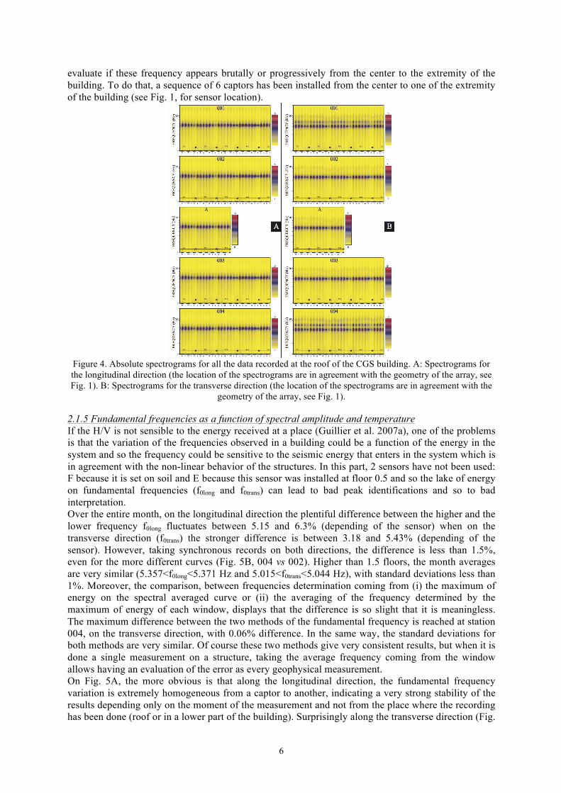
2.1.2 Weekly variations (Fig. 3B) Over a week, the amplitude at 5.44 Hz (f0long) displays a very strong variation in amplitude (from 3 to 15, i.e. a factor of variation of 5) when the curves below 2Hz and over 8 Hz display seems to have a stronger homogeneity even if the factor is the same (i.e. a factor of 4 with amplitude from 0.5 to 2). As written in Guillier et al. (2008) the weekly changes can be divided in two different periods: (i) from Saturday to Wednesday there is a strong day-night variation giving 5 times the daily variation (see above); (ii) from Thursday to Friday (the weekend) there is a weaker variation than during the workdays. As for daily variations, during the whole week, the f0long peak is always a steady peak as it is always the more energetic. 2.1.3 Monthly variations (Fig. 3C) The monthly variations of spectral amplitude display the same pattern as the daily-weekly variations (see above). 2.1.4 Monthly variations in the horizontal plan of the structure (Fig. 4) For the 5 sensors on the roof, the monthly variations observed are similar from a sensor direction to the others sensor on the same direction. On the longitudinal direction (Fig. 4A) the energy observed from a sensor to other sensor are similar, when on the transverse direction (Fig. 4B) the energy at the main frequency (f0trans) is stronger at the center of the building (A, 002 and 003) than on the extremities of the building (001 and 002), the center displaying 40% more energy. Moreover, on the transverse direction, on the extremities of the building, it appears a new stable-in-time frequency at 6.64 Hz, when this frequency is totally missing on the central building sensor (002, A and 003, Fig. 4B) on transverse direction, whatever the moment of the record and the size of observation of the curve. To best check this frequency apparition, it has been done a complementary survey in order to

6

evaluate if these frequency appears brutally or progressively from the center to the extremity of the building. To do that, a sequence of 6 captors has been installed from the center to one of the extremity of the building (see Fig. 1, for sensor location).

Figure 4. Absolute spectrograms for all the data recorded at the roof of the CGS building. A: Spectrograms for the longitudinal direction (the location of the spectrograms are in agreement with the geometry of the array, see Fig. 1). B: Spectrograms for the transverse direction (the location of the spectrograms are in agreement with the

geometry of the array, see Fig. 1).

2.1.5 Fundamental frequencies as a function of spectral amplitude and temperature If the H/V is not sensible to the energy received at a place (Guillier et al. 2007a), one of the problems is that the variation of the frequencies observed in a building could be a function of the energy in the system and so the frequency could be sensitive to the seismic energy that enters in the system which is in agreement with the non-linear behavior of the structures. In this part, 2 sensors have not been used: F because it is set on soil and E because this sensor was installed at floor 0.5 and so the lake of energy on fundamental frequencies (f0long and f0trans) can lead to bad peak identifications and so to bad interpretation. Over the entire month, on the longitudinal direction the plentiful difference between the higher and the lower frequency f0long fluctuates between 5.15 and 6.3% (depending of the sensor) when on the transverse direction (f0trans) the stronger difference is between 3.18 and 5.43% (depending of the sensor). However, taking synchronous records on both directions, the difference is less than 1.5%, even for the more different curves (Fig. 5B, 004 vs 002). Higher than 1.5 floors, the month averages are very similar (5.357<f0long<5.371 Hz and 5.015<f0trans<5.044 Hz), with standard deviations less than 1%. Moreover, the comparison, between frequencies determination coming from (i) the maximum of energy on the spectral averaged curve or (ii) the averaging of the frequency determined by the maximum of energy of each window, displays that the difference is so slight that it is meaningless. The maximum difference between the two methods of the fundamental frequency is reached at station 004, on the transverse direction, with 0.06% difference. In the same way, the standard deviations for both methods are very similar. Of course these two methods give very consistent results, but when it is done a single measurement on a structure, taking the average frequency coming from the window allows having an evaluation of the error as every geophysical measurement. On Fig. 5A, the more obvious is that along the longitudinal direction, the fundamental frequency variation is extremely homogeneous from a captor to another, indicating a very strong stability of the results depending only on the moment of the measurement and not from the place where the recording has been done (roof or in a lower part of the building). Surprisingly along the transverse direction (Fig.

Guillier et al. 7

5B), on 001 and 004, the frequency seems to be very perturbed, compared to the other sensors that are very homogeneous. The only difference between these two sensors and the other is that they are the more external sensors and display a lower energy (Fig. 4B), indicating that the transverse fundamental frequency determination can be fairly perturbed by the place chose for the measurement perhaps du to the presence of a torsion mode at 6.64 Hz. The daily-night variation of the fundamental frequencies appears clearly, especially on the longitudinal direction (Fig. 5A), as for the transverse direction (Fig. 5B), where this rippling exists but much more slightly (even for 001 and 004).

Figure 5. Variations of the fundamental frequencies of the CGS building. A: Longitudinal direction. B:

Transverse direction. On A and B, the first seven graphics display the evolution of the fundamental frequency in the specified direction recorded on 7 different captors. The eighth curve displays the variation of the amplitude (A(f0) assessed on the 004 and normalized. The last curve displays the evolution of the temperature during the entire month of study. A’: enlargement of the colored areas on A (4 days), allowing a better view of the peaks

marked by dashed lines. B’: enlargement of the colored areas on B (4 days), allowing a better view of the peaks marked by dashed lines.

At first glance, there is an agreement of the fundamental frequency daily-night variations with the daily-night oscillation observed for the amplitude of the fundamental frequency peaks observed on both directions. However, a zoom on 4 days (Fig. 5A’ and Fig. 5B’) allows to verify that the occurrence of maxima on the frequencies and on the amplitudes are not synchronous at all, as in general the maximum frequency peak oscillations is reached 5 hours later than the peak of energy. In the same way, it has been plotted the temperature variations for the same period (Fig. 5), variation that has the same global behavior that the frequencies or the amplitude oscillations. Fig 5A’ and 5B’ shows clearly that these thermal oscillations are asynchronous with the peaks of frequency, as in general the maximum frequency peak oscillations is reached 2 to 2.5 hours later than the thermal peak. Here, both thermal and energetic (from seismic noise) shapes have the same pattern that the fundamental frequency oscillation. However, a short time process as the seismic noise is unable to generate consequences five hour after its maximum of energy, as the energy is totally dissipated. On the contrary, the thermal processes that allow warming a structure do not have an immediate impact on the temperature of the structure as the heating process depends on the thermal conductivity and specific heat capacity of the medium (building) as well as the thermal inertia of the structure (Eumorfopoulou and Kontoleon, 2009). In general it is assumed that there is a thermal delay between thermal input of energy in a medium and the maximum of temperature in this medium, which is the thermal inertia, this time delay between maximum external temperature and internal one has

8

been precisely evaluated comparing the internal surface temperature and the external surface temperature (Di Perna et al. 2011) reaching to a time difference from 2 (for a RC building, Zhou et al. 2004) to 3 hours (for a masonry-concrete school, Di Perna et al. 2011). In the same way, the minimum of internal temperature is reached when the increase of the external temperature has started 2 to 3 hours before (Zhou et al. 2004; Di Perna et al. 2011). The time delay between the maximum of temperature inside and outside a building has of course a complex shape, which depends on the material used for the construction. For the CGS building in particular (and probably for all buildings), the thermal inertia gives finally a shift in time between the time of occurrence of the maximum external temperature (so the maximum of heat input in the building) and the maximum of internal temperature. The thermal process evidently cannot give an immediate response but a phase-shifted response as see in the CGS building. 2.2 Damping

Figure 6. Variations of the damping rate (ξ). A: Longitudinal direction. B: Transverse direction. On A and B, the first eight graphics display the evolution of ξ in the specified direction recorded on 8 different captors. The ninth curve displays the variation of ξ assessed on the 004 and normalized. The last curve displays the evolution of the

temperature during the entire month of study. A’: enlargement of the colored areas on A (4 days), allowing a better view of the peaks marked by dashed lines. B’: enlargement of the colored areas on B (4 days), allowing a

better view of the peaks marked by dashed lines. On A, for comparison, on the upper graph, the red curve corresponds to f0long obtained on 004 using the maximum of energy on the Fourier amplitude velocity spectra, when on B, for comparison, on the B second upper graph, the red curve corresponds to f0trans obtained on 002

using the maximum of energy on the Fourier amplitude velocity spectra

As for the fundamental frequencies, 2 sensors have not been used: F because it is set on soil and E because this sensor was installed at floor 0.5 and so, the lake of energy on fundamental frequencies (f0long and f0trans) can lead to bad peak identifications and so to bad damping frequency and rate. From the 17968 records, 35936 damping have been computed (vertical direction is not took into account), following the calculus parameters described before. The results are, for each record on both longitudinal and transverse directions, (i) a frequency where the damping is finally converging (ii) the damping rate (ξ) in itself. Taking into account the whole data processed for damping, the minimum window used is 3397 and the maximum 4711, giving enough data for an optima time staking. Over the survey, for the longitudinal direction, the averaged ξ varies between 2.750% and 3.013% (Fig. 6), depending on the sensor, with a standard deviation of 0.8%. For the transverse direction, the ξ rate varies between 2.579% and 2.629%, depending on the sensor, with a standard deviation of 0.6%,

Guillier et al. 9

except for 001 and 004 that have a higher damping rate, close to 3.0%, with a standard deviation upper than 1%. Along the longitudinal direction, during the complete survey (Fig. 6A), the damping rate stability, from a sensors to another one, is extremely robust, proving that the place of the measurement do not really care for this component. However, it is noticeable that all the ξ curves present very strong changes: collapses followed by strong increases (first Wednesday, second Tuesday, second Friday, second Sunday, third Tuesday) or brutal increase (last Sunday), but these “jumps” occur only in the early morning. Even if these “jumps” are meaningful (present on all the sensors, connected to different recorders) and represent a real temporally change in the dynamic properties of the building, the authors do not have any explanation of what it is occurring at these moments. For the longitudinal damping rate, its stability from a sensor to the other is very impressive, if 001 and 004 are excluded. As see before, for 001 and 004, their instability is probably coming from the presence of another peak close to the fundamental frequency (f0trans). As for the longitudinal damping, it occurs sometime some strong “jumps” on the curves (first Wednesday, second Tuesday, second Friday). These “jumps” are even present, synchronically, on the longitudinal damping curves, but the 3 others changes present later on the longitudinal direction do not appear on the transverse damping curves. As for the longitudinal damping, no physical explanation is actually suspected. Once more, at least on the longitudinal direction (Fig 6A), there is a clear day-night ξ oscillation that is clearly synchronous to the f0long oscillations (Fig. 6A, red curve), while on the transverse damping does not present any strong rippling (Fig. 6B). Yet again, zoom on the longitudinal direction (Fig. 6A’) illustrate that the ξ curves are neither synchronous to the maximum of energy nor to the temperature variations, when on the transverse direction (Fig 6B’) no peak can be defined on the damping curve. Finally, at least for the longitudinal direction it can be assumed that the damping rate is (i) linked to f0long and then (ii) probably linked to a phase-shifted thermal process.

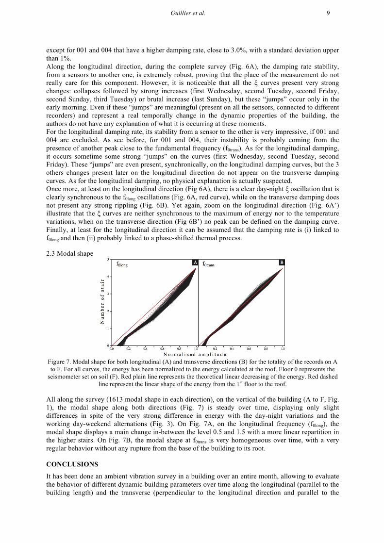
2.3 Modal shape

Figure 7. Modal shape for both longitudinal (A) and transverse directions (B) for the totality of the records on A to F. For all curves, the energy has been normalized to the energy calculated at the roof. Floor 0 represents the

seismometer set on soil (F). Red plain line represents the theoretical linear decreasing of the energy. Red dashed line represent the linear shape of the energy from the 1st floor to the roof.

All along the survey (1613 modal shape in each direction), on the vertical of the building (A to F, Fig. 1), the modal shape along both directions (Fig. 7) is steady over time, displaying only slight differences in spite of the very strong difference in energy with the day-night variations and the working day-weekend alternations (Fig. 3). On Fig. 7A, on the longitudinal frequency (f0long), the modal shape displays a main change in-between the level 0.5 and 1.5 with a more linear repartition in the higher stairs. On Fig. 7B, the modal shape at f0trans is very homogeneous over time, with a very regular behavior without any rupture from the base of the building to its root.

CONCLUSIONS

It has been done an ambient vibration survey in a building over an entire month, allowing to evaluate the behavior of different dynamic building parameters over time along the longitudinal (parallel to the building length) and the transverse (perpendicular to the longitudinal direction and parallel to the

10

building width) directions. These dynamic parameters are the following (i) the fundamental frequencies of the building on both directions (f0long and f0trans), (ii) the damping for both fundamental frequencies (f0long and f0trans) and (iii) the modal shape at f0long and f0trans. The goal of this study is to follow the evolution of these parameters during time and to evaluate if there is any common pattern over time. Moreover, this work deals with the possibility to compute the modal frequencies (f0long and f0trans) in a two different ways and to compare the different results. For the first method, the modal frequency is found by a “pick picking” method through the higher value of the Fourier amplitude velocity spectra leading to a modal frequency determination without any evaluation of the error on the frequency. The second method uses the Fourier amplitude velocity spectra of each stationary signal window where the maximum is found and then an averaged modal frequency is computed with an error evaluation. Both methods give strong coherent results, as the difference in the frequency between both methods does not exceed 0.06%. Moreover, the advantage of the second method is that the modal frequencies are defined with an estimation of the error, leading to not over-interpret any slight frequency variations. For this paper, it has been studied specifically the time length necessary to compute robust damping parameters (frequency and rate), length actually fixed to be over 10 periods of the studied frequency. It has been demonstrated that 10 periods are really too short in time to lead to a good damping parameters definition when length over 40 periods is much more convenient. The same test should be done on soil, as the damping is a critical argument for H/V reliability. The modal frequencies found for the CGS building are f0long=5.36 Hz and f0trans=5.03 Hz. For the fundamental frequencies of the building and whatever the direction, it appears clearly a strong oscillation displaying a clear day-night variation. Commonly, these daily frequency variations are interpreted as linked to the day-night variation of energy (Herak and Herak 2010), due to the different phases of the human life cycle (Guillier et al. 2007a). However and whatever the method used for frequency determination, the day-night oscillations in both directions do not affect the frequencies over 1%, which can be considered as very low impact day-night alternation. In this study, it appears that even if both frequency and energy curves display day-night oscillations, the two curves do not reach their maxima at the same time as the frequency maxima are reached about 5 hours later that the energy maxima. How the ambient vibration is a short-time process (as transient), the ambient vibration cannot be invoked to explain the time-shifted oscillations of 5 hours between frequency and energy. Similarly, the temperature variations have globally the same behavior than the fundamental frequencies (f0long and f0trans) and than the energy inside the building. But also with a shift in time, as the maxima temperature are reached 2 to 2.5 hours before the fundamental frequencies maxima and 2 to 2.5 later than the energy maxima in the building. Thermal processes, like the exposure to the sun and the heating, are strongly linked to thermal conductivity and specific heat capacity of the building as well as the thermal inertia of the structure, allowing a thermal delay of 2 to 4 hours between the external maxima temperature and the internal maxima medium temperature of the building (Kossecka and Kosny 2002). For the studied building and probably for all the buildings, and depending on the material used for the construction, the thermal inertia leads to a phase-shifted response of the internal temperature and then of the fundamental frequencies of the building. The frequencies found using damping processing for the CGS building are f0long-damp=5.38 Hz and f0trans-damp=5.08 Hz when the damping rate are 2.8% on the longitudinal direction and 2.6% on the transverse direction. On both building directions, the damping, whether for damped frequencies or damping rate, displays obvious oscillations synchronously with the f0long and f0trans oscillations, leading to very similar curve shapes coherent in time. So, there is a robust temporal relationship between the damping parameters (frequency and rate) and the frequencies coming from Fourier spectral amplitude analysis, i.e. the damping is probably strongly linked to the thermal processes that control the fundamental frequencies oscillations. However, even if the damping frequency and rate are coherent in time (oscillation), the damping rate is slightly unstable as in this building the damping errors are close to 25%, which is coherent with other in-situ results (Dunand, 2005; Herak and Herak 2010). However, the damping rate on both directions can display very strong “jumps” synchronous on the whole building, these “jumps” remaining enigmatic. Moreover, it is generally admitted that the variations of frequency (Trifunac et al. 2001a; 2001b) or damping (Jeary 1986; 1997) in a building are intimately linked to mobilization of structural imperfections as interfaces (walls, doors windows…), construction joints and cracks within the concrete. As the ambient vibrations stay in the elastic domain of the building, it is difficult to presume

Guillier et al. 11

that these imperfections can be activated by low-energy waves producing regular and asynchronous changes in the building. While the temperature variation of the building material is a good mechanism that explains the frequency oscillation and its observed time-shifted response. Finally, as these observations clearly prove that the level of energy of ambient vibration does not affect the studied dynamic parameters, and then, for low-strain induced by ambient vibration, the nonlinearity can be assumed as negligible. Of course, for higher solicitations (Hans et al 2005), the dynamic parameters of the building can be strongly affected entering in the nonlinearity domain. The modal shapes, critical dynamic parameter for building, calculated on both building directions, are extremely robust and do not present any significant changes over time. It should be noticed there that two sensors (001 and 004) on the transverse direction present very low-resolution curves in the frequency (normal or damping processings) and damping rate domains. This low-resolution is probably due to the presence of a torsion mode that appears only on these two sensors located on the extreme borders of the building. This torsion mode at 6.64 Hz most likely pollutes the transverse modal frequency. On the longitudinal direction of the CGS building, the results, for the dynamic parameters, are totally insensitive to the moment of the measurement and to the place where the measurement has been done. However, the transverse direction is much more complicated as depending on the location of the sensors, the results could be significantly different as for example the apparition of a new frequency can strongly perturb the damping rate determination, which can “jump” of a factor 4. In the same way, it is noticeable that the damping rate can present some “jumps” in time, leading to a bad determination of this parameter. Moreover, this problem of bad resolution, due to the pollution of the modal frequency by a close frequency, may lead to strong misinterpretations even for modal frequency picking. The observations done in this particular building clearly prove that the selection of the moment and the place of a single measurement are critical for any dynamic parameter study. Additionally, the presence of a torsion frequency at 6.64 Hz, totally missing in the center of the building, prove that the seismic joint does not play its role and that the building, which is separated in two blocks, is working as a single block.

REFERENCES

Andersen P, Brincker R, Peeters B, De Roeck G, Hermans L and Kramer C (2000) Comparison of system identification methods using ambient bridge test data. Proceeding of the 17th International Modal Analysis Conference (IMAC), Kissimmee, Florida, USA, 1035-1041.

Bendat JS and Piersol AG (1993) Engineering applications of correlation and spectral analysis. Willey New-York USA

Boutin C, Ibraim E, Hans S and Rousillon P (2001) Etude expériementale sur bâtiments reels. Technical report Association Française de Génie Parasismique (AFPS) and Ministère de l’Aménagement du Territoire et de l’Environnement, Paris, France.

Chatelain JL, Guéguen P, Guillier B, Fréchet J, Bondoux F, Sarrault J, Sulpice P and Neuville JM (2000) CityShark: A user-friendly instrument dedicated to ambient noise (microtremor) recording for site and building response studies. Seismological Research Letters 71(6):698–703.

Chatelain JL, Guillier B, Cara F, Duval A-M, Atakan K, Bard PY and the WP02 SESAME team (2008) Evaluation of the influence of experimental conditions on H/V results from ambient noise recordings. Bulletin of Earthquake Engineering 6 (1):33-74. doi: 10.1007/s10518-007-9040-7

Cole HA (1973) On-line Failure Detection and Damping Measurements of Aerospace Structures by Random Decrement Signature. NASA CR-2205.

Di Perna C, Stazi F, Ursini Casalena A, D’Orazio M (2011) Influence of the internal inertia of the building envelope on summertime comfort in buildings with high internal heat loads. Energy and Buildings 43:200-206. doi:10.1016/j.enbuild.2010.09.007

Dunand F (2005) Pertinence du bruit de fond sismique pour la caractérisation dynamique et l’aide au diagnostic sismique des structures de génie civil. PhD thesis, Université Joseph Fourier, Grenoble, France, 378p (in french).

Dunand F, Guéguen P, Bard P-Y, Rodgers J, Celebi M (2006) Comparison of the dynamic parameters extracted from weak, moderate and strong building motion. Proceeding 1st European Conference of Earthquake Engineering and Seismology, Genova, Switzerland paper 1021

Eumorfopoulou EA, Kontoleon KJ (2009) Experimental approach to the contribution of plant-covered walls to

12

the thermal behaviour of building envelopes. Building and Environment 44:1024-1038. Farsi MN, Guillier B, Chatelain JL, Zermout S (2009) Retrofitting and strengthening evaluation from stiffness

variations of a damaged building from ambient vibration recordings. In Increasing Seismic Safety by Combining Engineering, M. Mucciarelli et al. (eds.), NATO Science for Peace and Security, Series C: Environmental Security, Springer Sciences, 227-238.

Guillier B, Chatelain JL, Bonnefoy-Claudet S and Haghshenas E (2007a) Use of Ambient Noise: From Spectral Amplitude Variability to H/V Stability. Journal of Earthquake Engineering 11:1–18. doi: 10.1080/13632460701457249

Guillier B. Chatelain JL, Machane D, Farsi M (2007b) Évaluation de la rigidité d'un bâtiment en portiques auto-stables affecté par le séisme de Laalam (Bejaia-Algérie) du 20 mars 2006, 7th Colloque AFPS, 4-6 july 2007, Paris, France, Paper D-058.

Guillier B, Atakan K, Chatelain JL, Havskov J, Ohrnberger M, Cara F, Duval AM, Zacharopoulos S, Teves-Costa P, and the SESAME Team (2008) Influence of instruments on the H/V spectral ratios of ambient vibrations. Bulletin of Earthquake Engineering 6 (1):3-31. doi: 10.1007/s10518-007-9039-0

Hans S, Boutin C, Ibraim E, Roussillon P (2005) In Situ experiments and seismic analysis of existing buildings—part I: experimental investigations. Earthquake Engineering and Structural Dynamics 34(12):1513–1529

Ibrahim SR, Asmussen JC and Brincker R (1998) Vector triggering random decrement for high identification accuracy. Journal of Vibration and Acoustics 120:970-975.

Herak M and Herak D (2010) Continuous monitoring of dynamic parameters of the DGFSM building (Zagreb, Croatia). Bull Earthquake Engineering 8:657-669. doi 10.1007/s10518-009-9112-y

Jeary AP (1986) Damping in tall buildings – a mechamism and a predictor. Earthquake Engineering and Structural Dynamics 14:733-750.

Jeary AP (1997) Damping in structures. J Wind Eng Ind Aerodyn 72:345-355. Konno K and Ohmachi T (1998) Ground-motion characteristics estimated from spectral ratio between horizontal

and vertical components of microtremor. Bulletin of the Seismological Society of America 88 (1):228–241.

Kossecka E, Kosny J (2002) Influence of insulation configuration on heating and cooling loads in a continuously used building. Energy and Buildings 34:321-331.

Luong MP, Martin A, Liu H and De Parnay R (1992) Signature vibratoire des pylones électriques. Annales de l’Institut Technique du Bâtiment et des Travaux Publics, 501, Paris, France.

Michel C, Guéguen P, Lestuzzi P, Bard PY (2010) Comparison between seismic vulnerability models and experimental dynamic properties of existing buildings in France. Bull Earthquake Eng 8 :1295-1307. doi 10.1007/s10518-010-9185-7

Mucciarelli M, Gallipoli M, Di Giacomo D, Di Nota F, Nino E (2005) The influence of wind on measurements of seismic noise. Geophys J Int 161(2):303–308. doi:10.1111/j.1365-246X.2004.02561.x

Rodrigues J, Brincker R (2005) Application of Random Decrement Technique in Operational Modal Analysis . Proceedings of the 1st International Operational Modal Analysis Conference (IOMAC), Copenhagen, Denmark.

Satake N, Suda K, Arakawa T and Tamura Y (2003) Damping evaluation using full-scale data of buildings in Japan. Journal of Structural Engineering 129(4):470-477.

SESAME (2004) Guidelines for the implémentation of the H/Vspectral ratio technique on ambient vibrations. Measurements, processing and interpretation. European Commission – Research General Directorate Project No. EVG1-CT-2000-00026SESAME, report D23.12, http://SESAME-FP5.obs.ujf-grenoble.fr.

Todorovska M (2009) Soil-structure system identification of Millikan Library North–South response during four earthquakes (1970–2002): what caused the observed wandering of the system frequencies?. Bull Seismol Soc Am 99(2A):626–635

Trifunac MD (1972) Comparisons between ambient and forced vibration experiments. Earthquake Engineering and Structural Dynamics. 1 133-150.

Trifunac MD, Ivanovíc SS, Todorovska MI (2001a) Apparent periods of building. I: Fourier analysis. J Struct Eng 127:517–526. doi:10.1061/ (ASCE)0733- 9445(2001)127:5(517)

Trifunac MD, Ivanovíc SS, Todorovska MI (2001b) Apparent periods of building. II: time frequency analysis. J Struct Eng 127:527–537. doi:10.1061/ (ASCE)0733- 9445(2001)127:5(527)

Vandiver JK, Dunwoody AB, Campbell RB and Cook MF (1982) A mathematical basis for the random décrément vibration signature analysis technique. Journal of Mechanical Design 104:307-313.

Zhou N, Gao W, Nishida M, Kitayama H, Ojima T (2004) Field study on the thermal environment of passive cooling system in RC building. Energy and Buildings 36:1265-1272.

CONTINUOUS MONITORING OF AMBIENT VIBRATION … · 1 continuous monitoring of ambient vibration in...

Documents

Transcript of CONTINUOUS MONITORING OF AMBIENT VIBRATION … · 1 continuous monitoring of ambient vibration in...