
CONTINUOUS IMPLICIT HYBRID ONE-STEP … · Glory and Praise be unto the Almighty God who kept ......
170
CONTINUOUS IMPLICIT HYBRID ONE-STEP METHODS FOR THE SOLUTION OF INITIAL VALUE PROBLEMS OF GENERAL SECOND-ORDER ORDINARY DIFFERENTIAL EQUATIONS BY ANAKE, TIMOTHY ASHIBEL CUGP060192 September, 2011
-
Upload
nguyentuyen -
Category
Documents
-
view
220 -
download
0
Transcript of CONTINUOUS IMPLICIT HYBRID ONE-STEP … · Glory and Praise be unto the Almighty God who kept ......
CONTINUOUS IMPLICIT HYBRID ONE-STEP METHODS FOR
THE SOLUTION OF INITIAL VALUE PROBLEMS OF GENERAL
SECOND-ORDER ORDINARY DIFFERENTIAL EQUATIONS
BY
ANAKE, TIMOTHY ASHIBEL
CUGP060192
September, 2011

CONTINUOUS IMPLICIT HYBRID ONE-STEP METHODS FOR
THE SOLUTION OF INITIAL VALUE PROBLEMS OF GENERAL
SECOND-ORDER ORDINARY DIFFERENTIAL EQUATIONS
A Ph.D. Thesis
By
ANAKE, Timothy Ashibel
(Matric. Number: CUGP060192)
B.Sc Mathematics, University of Uyo, Nigeria
M.Sc Mathematics, University of Ibadan, Nigeria
Submitted to the School of Postgraduate Studies, Covenant University, Ota.
In Partial fulfilment of the requirements for the award of the degree of
Doctor of Philosophy in Mathematics
September, 2011
Declaration
I, Anake, Timothy Ashibel, (Matric. Number: CUGP060192) declare that this re-
search was carried out by me under the supervision of Prof. David O. Awoyemi of
the Department of Mathematical Sciences, Federal University of Technology, Akure
and Dr. Johnson O. Olaleru of the Department of Mathematics, University of Lagos,
Lagos. I attest that the thesis has not been presented either wholly or partly for the
award of any degree elsewhere. All sources of data and schorlarly information used
in this thesis are duly acknowledged.
Signature...............................
Date...........................
Anake, Timothy Ashibel
i

Certification
This is to certify that this Research was carried out by Anake, Timothy Ashibel,
(CUGP060192), in the Department of Mathematics, School of Natural and Applied
Sciences, College of Science and Technology, Covenant University, Ota, Nigeria.
———————————————– ———————————————–Prof D.O. Awoyemi Dr J.O. Olaleru
Supervisor Co-supervisorDepartment of Mathematical Sciences Department of Mathematics
Federal University of Technology University of LagosAkure, Nigeria Lagos, Nigeria.
———————————————– ———————————————–Dr. R.B. Adeniyi Prof. J.A. Gbadeyan
(External Examiner) Head of DepartmentDepartment of Mathematics Department of Mathematics
University of Ilorin, Covenant UniversityIlorin, Nigeria. Otta, Nigeria.
ii

Dedication
To my lovely wife, Winifred and the memory of my late brother, Chris (a.k.a cobra).
iii

Acknowledgment
Glory and Praise be unto the Almighty God who kept and strengthen me throughout
this research. Indeed, with Him, this work has become a reality.
I deeply appreciate my supervisor, Professor D.O. Awoyemi, who dedicatedly gave
me his shoulder to stand upon for the success of this work. A father and a prayer
partner among supervisors he has been to me. I am grateful also to my co-supervisor,
Dr. J.O. Olaleru, for his concern, encouragements, criticisms and directions. May
God bless both of them in very good measure.
I would like also to thank very profoundly, Prof. J.A. Gbadeyan, who as the head
of my department gave me sufficient attention and attended to my every need. To all
the staff of the department of Mathematics, Covenant University, I thank them for
their support and encouragement. At this point let me thank, immensely, Dr. A.O.
Adesanya for being such an inspiration, for those valuable contributions and for the
reliable friendship that we now share.
I appreciate all my friends and colleagues both in Covenant University and beyond
for their tireless encouragement especially, Prof. J. Katende, Prof. K.O. Okonjo, Dr.
N.U. Benson, Dr. G.O. Ana, Dr. G.U. Adie, and Mr. K.J. Bassey. Special thanks
to Mr. C. Nkiko for all the invaluable pieces of advice and counsel. I particularly
want to appreciate Dr. J. Ushie who inspired the path I have followed. He has been
a pillar of inspiration to me of which I am grateful.
I am grateful to Mrs. D.O. Awoyemi and her entire family for the warmth and
love they shared with me all through my stay in Akure. I thank them for wishing me
iv

well and may God bless them abundantly.
I want to appreciate Engr. Makinde of the Department of Petroleum Engineering,
Covenant University and Mr. Kayode of the Department of Computer Science, FUTA
who taught me FORTRAN programming and Mr. Gbenro for carefully typing this
thesis.
I appreciate every member of the Surveillance Team of CCU in Faith Terbanacle
of the Living Faith Church, Otta; as well as every member of the Full Gospel Busi-
nessmen Fellowship International especially my brethren in Golden Heart Chapter
and Iyana Iyesi Chapter. Their prayers and fellowship sustained me through this
research period and for this I am very grateful.
To my Parents, Mr. & Mrs. E. Anake; my brother, Frank; sisters, Jacinta, Lucia
and Schola; inlaws, Mr. & Mrs. U. Asuquo, and to all my relatives, I am grateful for
all their love and prayers.
I am most grateful to my lovely wife, Mrs. Winifred Anake, who weathered
the storm with love and support throughout this research. I appreciate her for the
understanding, prayers and cooperation. She is indeed my ’good thing’ and I love her
so much.
Finally, I thank the Vice Chancellor and the entire Management of Covenant
University for giving me this rare opportunity. I also thank my Bishop and Chancellor,
Dr. D. O. Oyedepo who created the platform upon which I have prospered. God bless
you sir.
Anake, Timothy A. 2011
v
Abstract
The numerical solutions of initial value problems of general second order ordinary
differential equations have been studied in this work. A new class of continuous
implicit hybrid one step methods capable of solving initial value problems of general
second order ordinary differential equations has been developed using the collocation
and interpolation technique on the power series approximate solution. The one step
method was augmented by the introduction of offstep points in order to circumvent
Dahlquist zero stability barrier and upgrade the order of consistency of the methods.
The new class of continuous implicit hybrid one step methods has the advantage of
easy change of step length and evaluation of functions at offstep points. The Block
method used to implement the main method guarantees that each discrete method
obtained from the simultaneous solution of the block has the same order of accuracy
as the main method. Hence, the new class of one step methods gives high order of
accuracy with very low error constants, gives large intervals of absolute stability, are
zero stable and converge. Sample examples of linear, nonlinear and stiff problems have
been used to test the performance of the methods as well as to compare computed
results and the associated errors with the exact solutions and errors of results obtained
from existing methods, respectively, in terms of step number and order of accuracy,
using written efficient computer codes.
vi
Contents
Declaration i
Certification ii
Dedication iii
Acknowledgment iv
Abstract vi
Contents vii
List of Tables xii
List of Figures xiii
List of Appendices xiv
1 Introduction 1
1.1 Preambles . . . . . . . . . . . . . . . . . . . . . . . . . . . . . . . . . 1
1.2 Existence and Uniqueness of Solutions of Initial Value Problems of
Ordinary Differential Equations . . . . . . . . . . . . . . . . . . . . . 3
1.3 Basic Features of Numerical Methods . . . . . . . . . . . . . . . . . . 4
1.4 Statement of the Problem . . . . . . . . . . . . . . . . . . . . . . . . 8
1.5 Aims and Objectives . . . . . . . . . . . . . . . . . . . . . . . . . . . 9
vii

1.6 Research Methodology . . . . . . . . . . . . . . . . . . . . . . . . . . 9
1.7 Contribution to Knowledge . . . . . . . . . . . . . . . . . . . . . . . . 10
1.8 Limitations of the Study . . . . . . . . . . . . . . . . . . . . . . . . . 10
2 Literature Review 12
2.1 Introduction . . . . . . . . . . . . . . . . . . . . . . . . . . . . . . . . 12
2.2 Review of Existing Methods . . . . . . . . . . . . . . . . . . . . . . . 12
3 Methodology 19
3.1 Introduction . . . . . . . . . . . . . . . . . . . . . . . . . . . . . . . . 19
3.2 Derivation of Methods . . . . . . . . . . . . . . . . . . . . . . . . . . 20
3.3 Specification of the Methods . . . . . . . . . . . . . . . . . . . . . . . 22
4 Analysis of the Methods 59
4.1 Introduction . . . . . . . . . . . . . . . . . . . . . . . . . . . . . . . . 59
4.1.1 Order and Error Constant . . . . . . . . . . . . . . . . . . . . 59
4.1.2 Consistency . . . . . . . . . . . . . . . . . . . . . . . . . . . . 62
4.1.3 Zero Stability . . . . . . . . . . . . . . . . . . . . . . . . . . . 63
4.1.4 Convergence . . . . . . . . . . . . . . . . . . . . . . . . . . . . 64
4.1.5 Region of Absolute Stability . . . . . . . . . . . . . . . . . . . 64
4.2 Analysis of the One Step Method with One Offstep Point . . . . . . . 66
4.2.1 Order and error constant . . . . . . . . . . . . . . . . . . . . . 66
4.2.2 Consistency . . . . . . . . . . . . . . . . . . . . . . . . . . . . 69
4.2.3 Zero Stability of One Step Method with One Offstep Point . . 70
4.2.4 Convergence . . . . . . . . . . . . . . . . . . . . . . . . . . . . 71
4.2.5 Region of Absolute Stability of the one step Method with One
Offstep Point . . . . . . . . . . . . . . . . . . . . . . . . . . . 71
4.3 Analysis of the One Step Method with Two Offstep Points . . . . . . 72
4.3.1 Order and Error Constant . . . . . . . . . . . . . . . . . . . . 72
viii
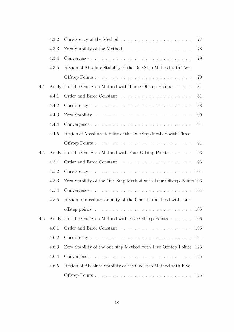
4.3.2 Consistency of the Method . . . . . . . . . . . . . . . . . . . . 77
4.3.3 Zero Stability of the Method . . . . . . . . . . . . . . . . . . . 78
4.3.4 Convergence . . . . . . . . . . . . . . . . . . . . . . . . . . . . 79
4.3.5 Region of Absolute Stability of the One Step Method with Two
Offstep Points . . . . . . . . . . . . . . . . . . . . . . . . . . . 79
4.4 Analysis of the One Step Method with Three Offstep Points . . . . . 81
4.4.1 Order and Error Constant . . . . . . . . . . . . . . . . . . . . 81
4.4.2 Consistency . . . . . . . . . . . . . . . . . . . . . . . . . . . . 88
4.4.3 Zero Stability . . . . . . . . . . . . . . . . . . . . . . . . . . . 90
4.4.4 Convergence . . . . . . . . . . . . . . . . . . . . . . . . . . . . 91
4.4.5 Region of Absolute stability of the One Step Method with Three
Offstep Points . . . . . . . . . . . . . . . . . . . . . . . . . . . 91
4.5 Analysis of the One Step Method with Four Offstep Points . . . . . . 93
4.5.1 Order and Error Constant . . . . . . . . . . . . . . . . . . . . 93
4.5.2 Consistency . . . . . . . . . . . . . . . . . . . . . . . . . . . . 101
4.5.3 Zero Stability of the One Step Method with Four Offstep Points 103
4.5.4 Convergence . . . . . . . . . . . . . . . . . . . . . . . . . . . . 104
4.5.5 Region of absolute stability of the One step method with four
offstep points . . . . . . . . . . . . . . . . . . . . . . . . . . . 105
4.6 Analysis of the One Step Method with Five Offstep Points . . . . . . 106
4.6.1 Order and Error Constant . . . . . . . . . . . . . . . . . . . . 106
4.6.2 Consistency . . . . . . . . . . . . . . . . . . . . . . . . . . . . 121
4.6.3 Zero Stability of the one step Method with Five Offstep Points 123
4.6.4 Convergence . . . . . . . . . . . . . . . . . . . . . . . . . . . . 125
4.6.5 Region of Absolute Stability of the One step Method with Five
Offstep Points . . . . . . . . . . . . . . . . . . . . . . . . . . . 125
ix
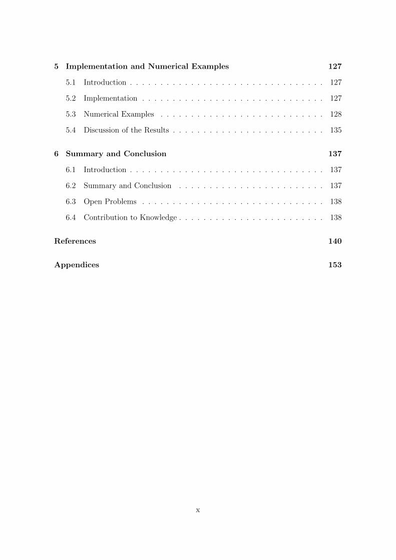
5 Implementation and Numerical Examples 127
5.1 Introduction . . . . . . . . . . . . . . . . . . . . . . . . . . . . . . . . 127
5.2 Implementation . . . . . . . . . . . . . . . . . . . . . . . . . . . . . . 127
5.3 Numerical Examples . . . . . . . . . . . . . . . . . . . . . . . . . . . 128
5.4 Discussion of the Results . . . . . . . . . . . . . . . . . . . . . . . . . 135
6 Summary and Conclusion 137
6.1 Introduction . . . . . . . . . . . . . . . . . . . . . . . . . . . . . . . . 137
6.2 Summary and Conclusion . . . . . . . . . . . . . . . . . . . . . . . . 137
6.3 Open Problems . . . . . . . . . . . . . . . . . . . . . . . . . . . . . . 138
6.4 Contribution to Knowledge . . . . . . . . . . . . . . . . . . . . . . . . 138
References 140
Appendices 153
x

List of Tables
Table 1. The boundaries of the region of absolute stability of the one step
1 offstep point method. . . . . . . . . . . . . . . . . . . . . . . . . . . 71
Table 2. The boundaries of the region of absolute stability of the one step
2 offstep points method. . . . . . . . . . . . . . . . . . . . . . . . . . 80
Table 3. The boundaries of the region of absolute stability of the one step
3 offstep points method. . . . . . . . . . . . . . . . . . . . . . . . . . 92
Table 4. The boundaries of the region of absolute stability of the one step
4 offstep points method. . . . . . . . . . . . . . . . . . . . . . . . . . 105
Table 5. The boundaries of the region of absolute stability the One Step 5
offstep points method. . . . . . . . . . . . . . . . . . . . . . . . . . . 125
Table 6. Summary of the analysis of the methods . . . . . . . . . . . . . . 126
Table 7. Showing the exact solutions and the computed results from the
proposed methods for Problem 1 . . . . . . . . . . . . . . . . . . . . . 130
Table 8. Comparing the absolute errors in the new methods to errors in
Awoyemi(1999) for Problem 1 . . . . . . . . . . . . . . . . . . . . . . 130
Table 9. Showing the exact solutions and the computed results from the
proposed methods for Problem 2 . . . . . . . . . . . . . . . . . . . . . 131
Table 10. Comparing the absolute errors in the new methods to errors in
Awoyemi(2001) for Problem 2 . . . . . . . . . . . . . . . . . . . . . . 131
Table 11. Showing the exact solutions and the computed results from the
proposed methods for Problem 3 . . . . . . . . . . . . . . . . . . . . . 132
xi
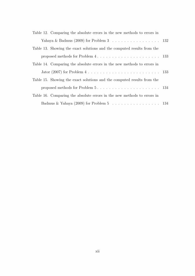
Table 12. Comparing the absolute errors in the new methods to errors in
Yahaya & Badmus (2009) for Problem 3 . . . . . . . . . . . . . . . . 132
Table 13. Showing the exact solutions and the computed results from the
proposed methods for Problem 4 . . . . . . . . . . . . . . . . . . . . . 133
Table 14. Comparing the absolute errors in the new methods to errors in
Jator (2007) for Problem 4 . . . . . . . . . . . . . . . . . . . . . . . . 133
Table 15. Showing the exact solutions and the computed results from the
proposed methods for Problem 5 . . . . . . . . . . . . . . . . . . . . . 134
Table 16. Comparing the absolute errors in the new methods to errors in
Badmus & Yahaya (2009) for Problem 5 . . . . . . . . . . . . . . . . 134
xii
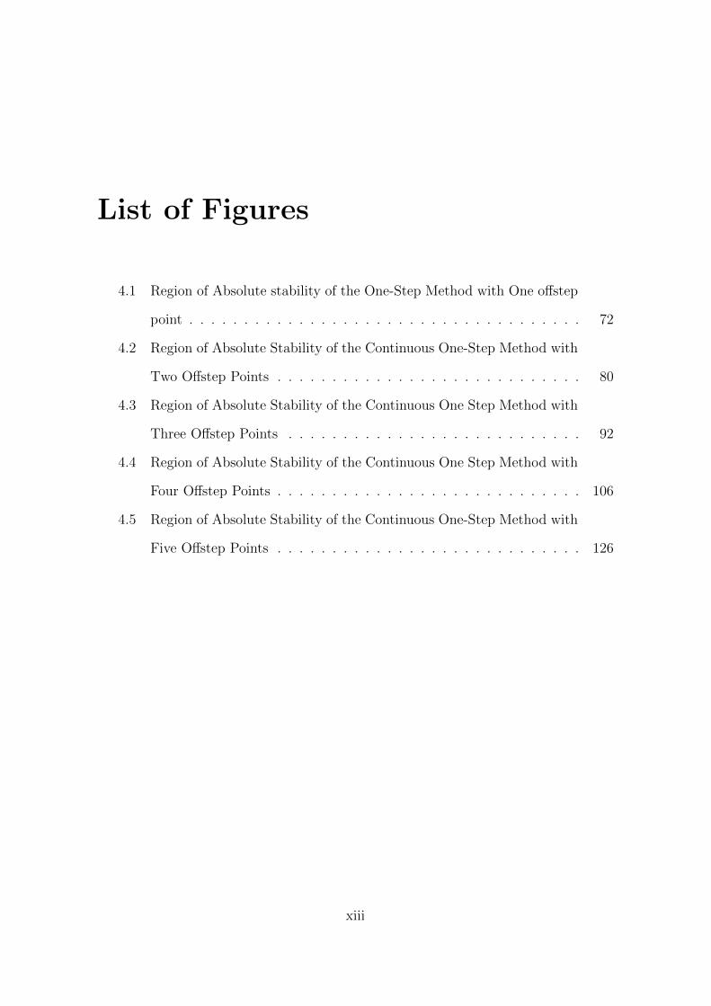
List of Figures
4.1 Region of Absolute stability of the One-Step Method with One offstep
point . . . . . . . . . . . . . . . . . . . . . . . . . . . . . . . . . . . . 72
4.2 Region of Absolute Stability of the Continuous One-Step Method with
Two Offstep Points . . . . . . . . . . . . . . . . . . . . . . . . . . . . 80
4.3 Region of Absolute Stability of the Continuous One Step Method with
Three Offstep Points . . . . . . . . . . . . . . . . . . . . . . . . . . . 92
4.4 Region of Absolute Stability of the Continuous One Step Method with
Four Offstep Points . . . . . . . . . . . . . . . . . . . . . . . . . . . . 106
4.5 Region of Absolute Stability of the Continuous One-Step Method with
Five Offstep Points . . . . . . . . . . . . . . . . . . . . . . . . . . . . 126
xiii

List of Appendices
Appendix I Computer Program of the 1S1HM for problem 1 159
Appendix II Computer Program of the 1S1HM for problem 2 160
Appendix III Computer Program of the 1S1HM for problem 3 161
Appendix IV Computer Program of the 1S1HM for problem 4 162
Appendix V Computer Program of the 1S1HM for problem 5 163
Appendix VI Computer Program of the 1S2HM for problem 1 164
Appendix VII Computer Program of the 1S2HM for problem 2 165
Appendix VIII Computer Program of the 1S2HM for problem 3 166
Appendix IX Computer Program of the 1S2HM for problem 4 167
Appendix X Computer Program of the 1S2HM for problem 5 168
Appendix XI Computer Program of the 1S3HM for problem 1 169
Appendix XII Computer Program of the 1S3HM for problem 2 170
Appendix XIII Computer Program of the 1S3HM for problem 3 171
Appendix XIV Computer Program of the 1S3HM for problem 4 172
Appendix XV Computer Program of the 1S3HM for problem 5 173
xiv

Appendix XVI Computer Program of the 1S4HM for problem 1 174
Appendix XVII Computer Program of the 1S4HM for problem 2 176
Appendix XVIII Computer Program of the 1S4HM for problem 3 178
Appendix XIX Computer Program of the 1S4HM for problem 4 180
Appendix XX Computer Program of the 1S4HM for problem 5 182
Appendix XX1 Computer Program of the 1S5HM for problem 1 184
Appendix XXII Computer Program of the 1S5HM for problem 2 186
Appendix XXIII Computer Program of the 1S5HM for problem 3 188
Appendix XXIV Computer Program of the 1S5HM for problem 4 190
Appendix XXV Computer Program of the 1S5HM for problem 5 192
xv

Chapter 1
Introduction
1.1 Preambles
In science and engineering, usually mathematical models are developed to help in
the understanding of physical phenomena. These models often yield equations that
contain some derivatives of an unknown function of one or several variables. Such
equations are called differential equations. Differential equations do not only arise
in the physical sciences but also in diverse fields as economics, medicine, psychology,
operation research and even in areas such as biology and anthropology.
Interestingly, differential equations arising from the modeling of physical phe-
nomena, often do not have analytic solutions. Hence, the development of numerical
methods to obtain approximate solutions becomes necessary. To that extent, several
numerical methods such as finite difference methods, finite element methods and fi-
nite volume methods, among others, have been developed based on the nature and
type of the differential equation to be solved.
A differential equation in which the unknown function is a function of two or
more independent variable is called partial differential equation. Those in which the
unknown function is a function of only one independent variable are called ordinary
differential equations. This work concerns the study of numerical solutions of the
latter.
In particular, finite difference methods have excelled for the numerical treatment
1

of ordinary differential equations especially since the advent of digital computers.
The development of algorithms has been largely guided by convergence theorems of
Dahlquist (1956, 1959, 1963, 1978) as well as the treatises of Henrici (1962) and
Stetter (1973), (Fatunla, 1988).
The development of numerical methods for the solution of Initial Value Problems
(IVPs) of Ordinary Differential Equations (ODEs) of the form
y(µ) = f(x, y, y(1), . . . , y(µ−1)), y(a) = η0, y(1)(a) = η1, . . . , y
(µ−1)(a) = ηµ−1 (1.1.1)
on the interval [a, b] has given rise to two major discrete variable methods namely; one
step (or single step) methods and multistep methods especially the Linear Multistep
Methods (LMMs).
One step methods include the Euler’s methods, the Runge-Kutta methods, the
theta methods, etc. These methods are only suitable for the solutions of first order
IVPs of ODEs because of their very low order of accuracy. In order to develop
higher order one step methods such as Runge-Kutta methods, the efficiency of Euler
methods, in terms of the number of function evaluations per step, is sacrificed since
more function evaluations is required. Hence, solving (1.1.1) using any one step
method means reducing it to an equivalent system of first order IVPs of ODEs which
increases the dimension of the problem thus increasing its scale. The result is that
one step methods become time-consuming for large scale problems and give results
of low accuracy.
Linear multistep methods on the other hand, include methods such as Adam-
Bashforth method, Adam-Moulton method, and Numerov method. These methods
give high order of accuracy and are suitable for the direct solution of (1.1.1) without
necessarily reducing it to an equivalent system of first order IVPs of ODEs. Linear
multistep methods are not as efficient, in terms of function evaluations, as the one
step method and also require some values to start the integration process.
This research work is concerned with the development of continuous implicit hy-
2

brid one step methods. These methods combine the efficiency of one step methods
and the high order of accuracy of multistep methods to solve the particular case of
(1.1.1) when n = 2.
Basically, the thesis consists of six chapters. Chapter one contains the intro-
duction, basic features of ordinary differential equations, basic concept of numerical
methods, justification of the study, aims and objectives of the study, the methodology
of the study, expected contributions to knowledge and limitations to the study. In
Chapter two, relevant and related literature are reviewed. Chapter three contains
detailed discussions on the methodology and derivation of the methods. Chapter
four contains analysis of basic properties of the methods developed as well as an in-
vestigation of their weak stability properties. In Chapter five, sample problems are
used to test the performance of the one step methods developed and the computed
solutions are compared with the exact solutions of the sample problems and the re-
sults from existing linear multistep methods. The results are also discussed in this
chapter. Finally, Chapter six contains summary, conclusion, recommendations and
contributions to the body of knowledge. Open problems have also been suggested,
followed by references and appendices.
In what follows, the existence and uniqueness of the solutions of higher order
ordinary differential equations is discussed.
1.2 Existence and Uniqueness of Solutions of Ini-
tial Value Problems of Ordinary Differential
Equations
In this section, existence and uniqueness theorem by Wend (1967) is adopted to es-
tablish the existence and uniqueness of solutions of (1.1.1). The proof of the theorem
can be found in Wend (1967 and 1969).
3
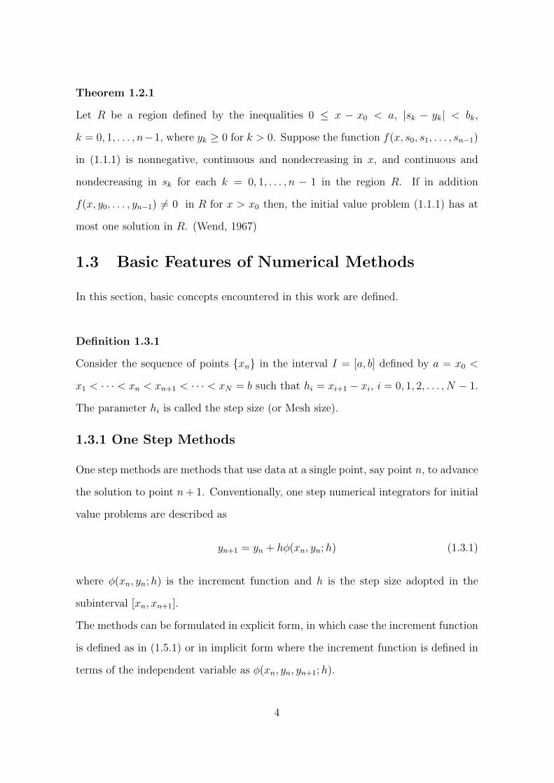
Theorem 1.2.1
Let R be a region defined by the inequalities 0 ≤ x − x0 < a, |sk − yk| < bk,
k = 0, 1, . . . , n−1, where yk ≥ 0 for k > 0. Suppose the function f(x, s0, s1, . . . , sn−1)
in (1.1.1) is nonnegative, continuous and nondecreasing in x, and continuous and
nondecreasing in sk for each k = 0, 1, . . . , n − 1 in the region R. If in addition
f(x, y0, . . . , yn−1) 6= 0 in R for x > x0 then, the initial value problem (1.1.1) has at
most one solution in R. (Wend, 1967)
1.3 Basic Features of Numerical Methods
In this section, basic concepts encountered in this work are defined.
Definition 1.3.1
Consider the sequence of points xn in the interval I = [a, b] defined by a = x0 <
x1 < · · · < xn < xn+1 < · · · < xN = b such that hi = xi+1 − xi, i = 0, 1, 2, . . . , N − 1.
The parameter hi is called the step size (or Mesh size).
1.3.1 One Step Methods
One step methods are methods that use data at a single point, say point n, to advance
the solution to point n+ 1. Conventionally, one step numerical integrators for initial
value problems are described as
yn+1 = yn + hφ(xn, yn;h) (1.3.1)
where φ(xn, yn;h) is the increment function and h is the step size adopted in the
subinterval [xn, xn+1].
The methods can be formulated in explicit form, in which case the increment function
is defined as in (1.5.1) or in implicit form where the increment function is defined in
terms of the independent variable as φ(xn, yn, yn+1;h).
4
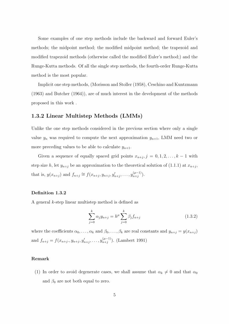
Some examples of one step methods include the backward and forward Euler’s
methods; the midpoint method; the modified midpoint method; the trapezoid and
modified trapezoid methods (otherwise called the modified Euler’s method;) and the
Runge-Kutta methods. Of all the single step methods, the fourth-order Runge-Kutta
method is the most popular.
Implicit one step methods, (Morisson and Stoller (1958), Ceschino and Kuntzmann
(1963) and Butcher (1964)), are of much interest in the development of the methods
proposed in this work .
1.3.2 Linear Multistep Methods (LMMs)
Unlike the one step methods considered in the previous section where only a single
value yn was required to compute the next approximation yn+1, LMM need two or
more preceding values to be able to calculate yn+1.
Given a sequence of equally spaced grid points xn+j, j = 0, 1, 2, . . . , k − 1 with
step size h, let yn+j be an approximation to the theoretical solution of (1.1.1) at xn+j,
that is, y(xn+j) and fn+j ∼= f(xn+j, yn+j, y′n+j, . . . , y
(µ−1)n+j ).
Definition 1.3.2
A general k-step linear multistep method is defined as
k∑j=0
αjyn+j = hµk∑j=0
βjfn+j (1.3.2)
where the coefficients α0, . . . , αk and β0, . . . , βk are real constants and yn+j = y(xn+j)
and fn+j = f(xn+j., yn+j, y′n+j, . . . , y
(µ−1)n+j ). (Lambert 1991)
Remark
(1) In order to avoid degenerate cases, we shall assume that αk 6= 0 and that α0
and β0 are not both equal to zero.
5

(2) If βk = 0 then yn+k is obtained explicitly from previous values of yn+j and fn+j,
and the k-step method is said to be explicit.
On the other hand, if βk 6= 0 then yn+k appears not only on the left-hand side
of (1.3.2) but also on the right within fn+k; due to this implicit dependence on
yn+k, the method is then called implicit.
(3) The k-step LMM (1.3.2) is called linear because it involves only linear combi-
nations of the yn+j and the fn+j.
(4) For the purpose of this work, the coefficients αj’s and βj’s in (1.3.2) are consid-
ered as real and continuous. In this case, (1.3.2) is referred to as Continuous
Linear Multistep Methods,(CLMMs), (Awoyemi, 1992).
1.3.3 Hybrid Methods
Continuous Linear Multistep Methods (CLMMs) when compared to Runge-Kutta
methods have the advantage of being more efficient in terms of accuracy and weak
stability properties for a given number of function evaluations per step, but have
the disadvantage of requiring starting values and special procedures for changing step
sizes. The difficulties could be addressed if the step number of the CLMMs is reduced,
the only obstacle to this is in satisfying the “zero stability barrier” of Dahlquist (1959
and 1963). This barrier implies that a zero stable CLMMs is at best of order p = k+1
for k odd and of order p = k + 2 for even k. Incorporating function evaluation at
offstep points affords the opportunity of circumventing the “zero stability barrier”.
According to Lambert (1973), this technique was used independently by Gragg and
Stetter (1964), Gear (1964) and later by Butcher (1965). The beauty of this method,
which was named “Hybrid methods” by Gear (1964), is that while retaining certain
characteristics of CLMMs, hybrid methods share with Runge-Kutta methods the
property of utilizing data at off step points and the flexibility of changing step length.
6

Definition 1.3.3
A k-step hybrid formula is defined as
k∑j=0
αjyn+j = h
k∑j=0
βjfn+j + h′βνfn+ν (1.3.3)
where αk = +1, α0 and β0 are both not zero, ν /∈ 0, 1, . . . , k, yn+j = y(xn + jh) and
fn+ν = f(xn+ν , yn+ν). (Lambert, 1973)
Remark
For the purpose of this work, the coefficients αj, βj, βν and αν will be real and
continuous functions and fn+j = f(xn+j, yn+j, y′n+j).
1.3.4 Block Methods
A block method is formulated in terms of linear multistep methods. It preserves the
traditional advantage of one step methods, of being self-starting and permitting easy
change of step length (Lambert, 1973). Their advantage over Runge-Kutta methods
lies in the fact that they are less expensive in terms of the number of functions
evaluation for a given order. The method generates simultaneous solutions at all grid
points.
According to Chu and Hamilton (1987) a block method can be defined as follows:
Definition 1.3.4
Let Ym and Fm be defined by Ym = (yn, yn+1, . . . , yn+r−1)T , Fm = (fn, fn+1, . . . , fn+r−1)
T .
Then a general k-block, r-point block method is a matrix of finite difference equation
of the form
Ym =k∑j=1
AiYm−i + hk∑i=0
BiFm−i (1.3.4)
where all the Ai’s and Bi’s are properly chosen r × r matrix coefficients and m =
0, 1, 2, . . . represents the block number, n = mr is the first step number of the mth
7

block and r is the proposed block size.
Remark
In the sequel, (1.3.4) will be redefined to suit the purpose of this research later in
Chapter three.
1.4 Statement of the Problem
Conventional methods of solving higher order IVPs of general ODEs by reduction
order method has been reported to have setbacks such as computational burden,
complication in writing computer programs and resultant wastage of computer time
(Awoyemi, 1992) and the inability of the method to utilize additional information
associated with a specific ODEs such as the oscillatory nature of the solution (Vigo-
Aguiar and Ramos, 2006) occasioned by the increased dimension of the problem and
the low order of accuracy of the methods employed to solve the system of first-order
IVPs of ODEs.
Equivalently, linear multistep methods implemented by the predictor-corrector
mode have been found to be very expensive to implement in terms of the number of
function evaluations per step, the predictors often have lower order of accuracy than
the correctors especially when all the step and offstep points are used for collocation
and interpolation.
The application of hybrid methods in the linear multistep methods, to achieve
reduction in the step number, in the predictor corrector mode is compounded by the
need to develop predictors for the evaluation of the corrector at offstep points making
the approach even more tedious and time consuming (Lambert, 1991).
The introduction of block methods to cushion the challenges associated with linear
multistep methods implemented in the predictor-corrector mode has largely been
concentrated in solving IVPs of special ODEs.
8

In view of the foregoing, this research is motivated by the need to address the set
backs associated with the existing methods, by developing a method that harnesses
the beautiful properties of these existing methods. Such a method would be less
expensive, in terms of the number of functions evaluation per step; highly efficient in
terms of accuracy and error term; flexible in change of step size; possess better rate
of convergence and weak stability properties; and very easy to program resulting in
economy of computer time.
1.5 Aims and Objectives
The aim of this research is to develop continuous implicit hybrid one step meth-
ods for the direct solution of initial value problems of general second order ordinary
differential equations. To achieve this aim, the following objectives were outlined:
(i) to develop continuous implicit one step methods by collocating and interpolating
at both the step and offstep points;
(ii) to implement the methods without the rigor of developing predictors separately;
(iii) to analyse basic properties of the method developed which include order, con-
sistency, zero stability, convergence and region of absolute stability;
(iv) to write computer programs, that are easy to implement; and
(v) to test the performance of the new methods for accuracy and efficiency.
1.6 Research Methodology
Power series polynomial of the form
y(x) =k∑j=0
ajxj (1.7.1)
9
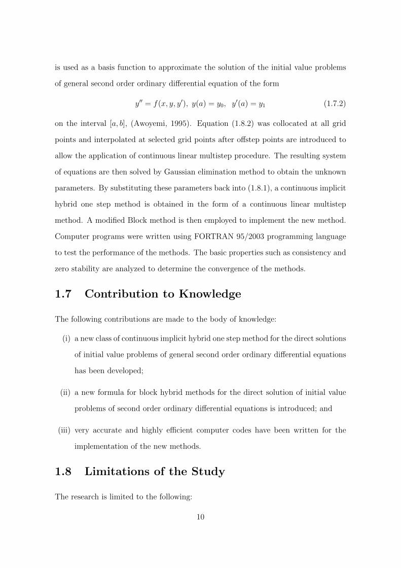
is used as a basis function to approximate the solution of the initial value problems
of general second order ordinary differential equation of the form
y′′ = f(x, y, y′), y(a) = y0, y′(a) = y1 (1.7.2)
on the interval [a, b], (Awoyemi, 1995). Equation (1.8.2) was collocated at all grid
points and interpolated at selected grid points after offstep points are introduced to
allow the application of continuous linear multistep procedure. The resulting system
of equations are then solved by Gaussian elimination method to obtain the unknown
parameters. By substituting these parameters back into (1.8.1), a continuous implicit
hybrid one step method is obtained in the form of a continuous linear multistep
method. A modified Block method is then employed to implement the new method.
Computer programs were written using FORTRAN 95/2003 programming language
to test the performance of the methods. The basic properties such as consistency and
zero stability are analyzed to determine the convergence of the methods.
1.7 Contribution to Knowledge
The following contributions are made to the body of knowledge:
(i) a new class of continuous implicit hybrid one step method for the direct solutions
of initial value problems of general second order ordinary differential equations
has been developed;
(ii) a new formula for block hybrid methods for the direct solution of initial value
problems of second order ordinary differential equations is introduced; and
(iii) very accurate and highly efficient computer codes have been written for the
implementation of the new methods.
1.8 Limitations of the Study
The research is limited to the following:
10

(i) only continuously differentiable functions in the interval of integration were
considered;
(ii) the basis function considered in this work is the power series polynomial in view
of its smoothness;
(iii) the research work adopted only continuous hybrid linear multistep methods
where the step number k = 1;
(iv) only implicit block methods were adopted in this research work.
In the next chapter, some literatures on existing numerical methods for solving
IVPs of higher order ordinary ordinary differential equations were reviewed.
11

Chapter 2
Literature Review
2.1 Introduction
The desire to obtain more accurate approximate solutions to mathematical models,
arising from science, engineering and even social sciences, in the form of ordinary
differential equations which do not have analytical solutions, has led many scholars
to propose several different numerical methods.
In this chapter, some of the many contributions available in the literature are
reviewed. Specifically, those numerical methods for the solution of (1.1.1) and in
particular the special case (1.8.2), when n = 2 is considered.
2.2 Review of Existing Methods
In most applications, (1.1.1) is solved by reduction to an equivalent system of first
order ordinary differential equations of the form
y′ = f(x, y), y(a) = µ; a ≤ x ≤ b;x, y ∈ Rn and f ∈ C1[a, b] (2.2.1)
for any appropriate numerical method to be employed to solve the resultant system.
The approach is extensively discussed by some prominent authors such as Lambert
(1973, 1991), Goult, Hoskins,and Pratt (1973), Lambert and Watson (1976), Do-
des (1978), Jain, Kambo and Rakesh (1984), Ixaru (1984), Kadalbajoo and Raman
(1986), Jacques and Judd (1987), Fatunla (1988), Sarafyan (1990), Bun and Vasil’Yer
12

(1992), Awoyemi (1992), Onumanyi, Awoyemi, Jator, and Sirisena (1994), Brugnano
and Trigiante (1998), Jator (2001), Juan (2001), among others. In spite of the suc-
cess of this approach, there are setbacks. For example, writing computer programs
for these methods is often cumbersome especially when subroutines are incorporated
to supply starting values required for the methods. The consequences are in longer
computer time and more human effort, (Awoyemi,1992). In addition, this method
does not utilize additional information associated with specific ordinary differential
equations, such as the oscillatory nature of the solution, (Vigo-Aguilar and Ramos,
2006). Furthermore, according to Bun and Vasil’Yer (1992), a more serious disad-
vantage of the method is the fact that the given system of equations to be solved
cannot be solved explicitly with respect to the derivatives of the highest order, (Kay-
ode, 2004). For these reasons, this method is inefficient and not suitbale for general
purpose applications.
Rutishauser (1960), examined the direct solution of (1.1.1) and its equivalent first
order initial value problems and concluded that the choice of approach depends on the
particular problem under consideration. Many other Scholars such as Henrici (1962),
Gear (1971), Hairer and Wanner (1976), Jeltsch (1976), Twizel and Khaliq (1984),
Chawla and Sharma (1985), Fatunla (1988), Taiwo and Onumanyi (1991), Awoyemi
(1995, 1998, 1999,2001, 2003, 2005), Simos (2002), Onumanyi Sirisena and Chollom
(2001), Awoyemi and Kayode (2005), Kayode (2004, 2005 and 2009), and Yusuph
and Onumanyi (2005), Vigo-Aguiar and Ramos (2006), Adesanya, Anake and Udoh
(2008), Adesanya, Anake and Oghoyon (2009), etc, suggested in the literature that a
better alternative is to solve (1.1.1) directly without first reducing it to a system of
first order ordinary differential equations.
In particular, this work is concerned only with the direct solutions of (1.1.1) for
n = 2 without reducing it to an equivalent system of first order equations. However,
many Scholars such as Henrici (1962), Jeltsch (1976), Twizel and Khaliq (1984),
13

Awoyemi (1998), Simos (2002), and Yusuph and Onumanyi (2005), have devoted a
lot of attention to the development of various methods for solving directly the special
second order initial value problems of the form
y′′ = f(x, y), y(a) = µ0, y′(a) = µ1, (2.2.2)
which is the mathematical formulation for systems without dissipation. Nystrom
for instance, considered a step-by-step method based on the classical Runge-Kutta
methods, (Fatunla, 1988). Later, Hairer and Wanner (1976) developed Nystrom-type
methods for (2.2.2) in which they listed order conditions for the determination of the
parameters of the method. Gear (1971), Hairer (1979), Chawla and Sharma (1981),
independently developed explicit and implicit Runge-Kutta Nystrom type methods.
Dormand and Prince (1987) also developed two classes of embedded Runge-Kutta-
Nystrom methods for the direct solution of (2.2.2). First step methods were also
discussed by Gonzalez and Thompson (1997) as starting values required to implement
the Numerov method for the direct solution of (2.2.2).
In the literature also, Henrici (1962) and later Lambert (1973) postulated the
derivation of linear multistep methods with constant coefficients for solving (2.2.2).
Fatunla (1984, 1985, 1988) developed P -stable one-leg constant coefficients linear
multistep method in which Pade approximation was used to realize his methods for
the solution of (2.2.2). Vigo-Aguilar and Ramos (2006) in their contribution dis-
cussed variable step size multistep schemes based on the Falkner method and directly
applied it to eqn.(2.2.2) in predictor-corrector mode. More on LMM can be found
in Lie and Norsett (1989), Enright (1974), Dahlquist (1978), Enright and Addison
(1984), Chawla and Rao (1985), Chawla and McKee (1986), to mention a few. The
procedure they adopted for this class of methods is such that the resultant methods
are not continuous, and therefore it is impossible to find the first and higher order
derivatives of y with respect to x; and so the scope of this class of methods is limited
in application, (Awoyemi, 2001).
14
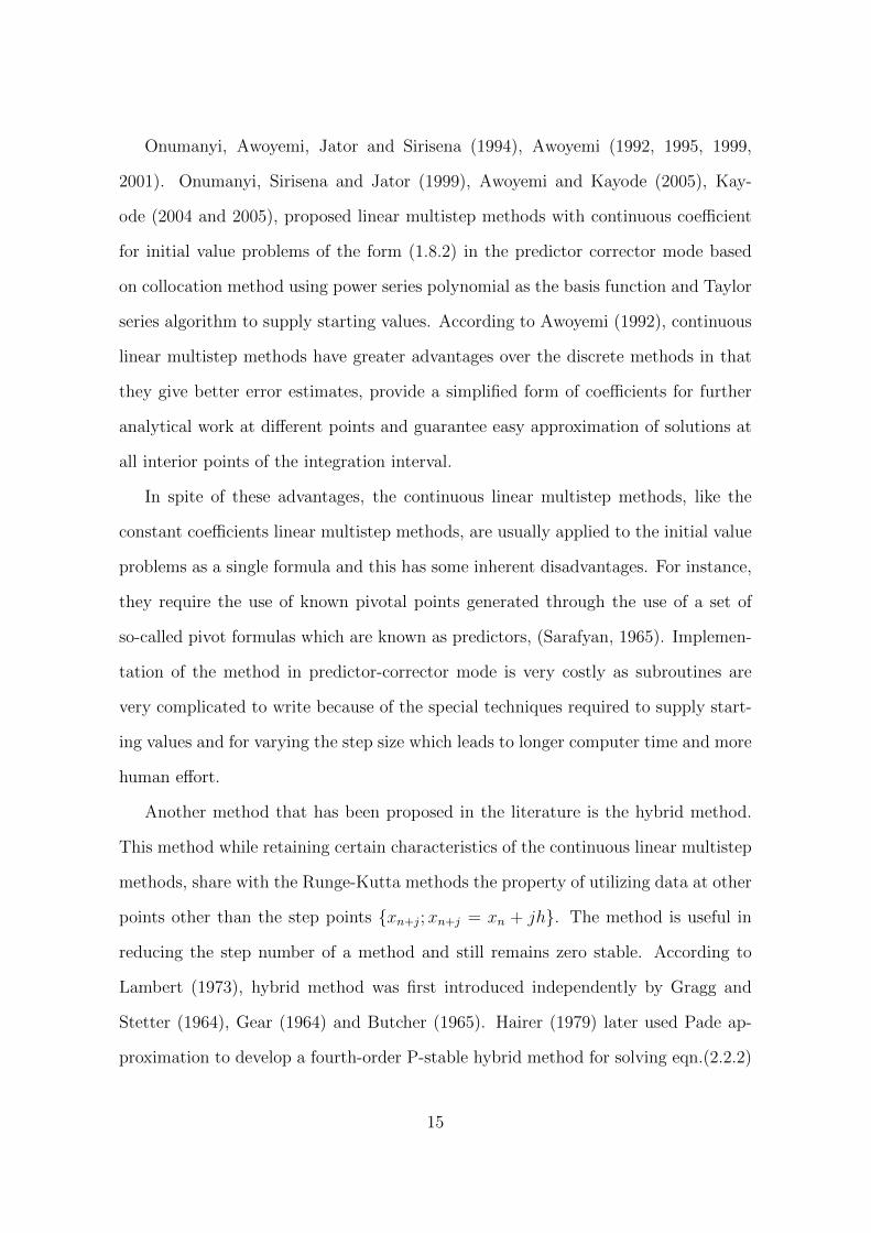
Onumanyi, Awoyemi, Jator and Sirisena (1994), Awoyemi (1992, 1995, 1999,
2001). Onumanyi, Sirisena and Jator (1999), Awoyemi and Kayode (2005), Kay-
ode (2004 and 2005), proposed linear multistep methods with continuous coefficient
for initial value problems of the form (1.8.2) in the predictor corrector mode based
on collocation method using power series polynomial as the basis function and Taylor
series algorithm to supply starting values. According to Awoyemi (1992), continuous
linear multistep methods have greater advantages over the discrete methods in that
they give better error estimates, provide a simplified form of coefficients for further
analytical work at different points and guarantee easy approximation of solutions at
all interior points of the integration interval.
In spite of these advantages, the continuous linear multistep methods, like the
constant coefficients linear multistep methods, are usually applied to the initial value
problems as a single formula and this has some inherent disadvantages. For instance,
they require the use of known pivotal points generated through the use of a set of
so-called pivot formulas which are known as predictors, (Sarafyan, 1965). Implemen-
tation of the method in predictor-corrector mode is very costly as subroutines are
very complicated to write because of the special techniques required to supply start-
ing values and for varying the step size which leads to longer computer time and more
human effort.
Another method that has been proposed in the literature is the hybrid method.
This method while retaining certain characteristics of the continuous linear multistep
methods, share with the Runge-Kutta methods the property of utilizing data at other
points other than the step points xn+j;xn+j = xn + jh. The method is useful in
reducing the step number of a method and still remains zero stable. According to
Lambert (1973), hybrid method was first introduced independently by Gragg and
Stetter (1964), Gear (1964) and Butcher (1965). Hairer (1979) later used Pade ap-
proximation to develop a fourth-order P-stable hybrid method for solving eqn.(2.2.2)
15

using one offpoint. In the same spirit as Hairer, Chawla (1981) and Cash (1981)
independently showed that the zero stability barrier imposed by Lambert (1973) and
Dahlquist (1978) could indeed be circumvented by considering two step hybrid meth-
ods. The result of their exposition was the development of fourth and sixth order
P-stable methods. Fatunla (1984) also used Pade approximation to develop one-leg
hybrid multistep method. However, Jain et al. (1984) in developing their sixth-order
symmetric multistep method for period IVP of type (2.2.2), observed that the cost of
implementing the method by Cash (1981) was high due to many function evaluations
per iteration. Awoyemi (1995) adopted the method and proposed a two-step hybrid
multistep method with continuous coefficients for the solution of (2.2.2) based on
collocation at selected grid points and using off-grid points to upgrade the order of
the method and to provide one additional interpolation point and implemented on
the hybrid predictor-corrector mode. Later, Adee, Onumanyi, Sirisena and Yahaya
(2005) in solving (2.2.2) used hybrid formula of order four to generate starting values
for Numerov method. D’Ambrosio, Ferro and Paternoster (2009) on the other hand
proposed a two step hybrid collocation method based on Butcher’s general linear
methods (GLM) to solve (2.2.2). Other Scholars who have studied hybrid methods
include; Onumanyi et al. (2001), Yahaya and Badmus (2009), etc. According to Lam-
bert (1973), hybrid method is not a method in its own right since special predictors
were required to estimate the solution at the offstep point and the derivative function
as well.
In view of all the disadvantages mentioned above, many researchers concentrated
efforts on advancing the numerical solution of initial value problems of ordinary dif-
ferential equations. One of the outcomes is the development of a class of methods
called Block method. The method simultaneously generates approximations at dif-
ferent grid points in the interval of integration and is less expensive in terms of the
number of function evaluations compared to the linear multistep methods or Runge-
16

Kutta methods. This method was first proposed by Milne (1953), who advocated
their use only as a means of obtaining starting values for predictor-corrector algo-
rithm. This was considered in the same light by Sarafyan (1965) however, Rosser
(1967) later developed Milne’s proposal to algorithms suitable for general use. Using
Rosser’s approach, Lambert (1973), developed a two-step fourth-order explicit block
method. Earlier on, implicit block methods had been proposed. For instance, an ex-
ample due to Clippinger and Dimsdale in Grabbe, Ramo and Woolridge (1958) was
analyzed by Shampine and Watts (1969) as implicit one step block method. Since
then, many contributions on block methods with different approaches have been pro-
posed in the literatures in recent years. For instance, Chu and Hamilton (1987)
suggested a generalization of the linear multistep method to a class of multi-block
methods where step values are all obtained together in a single block advance ac-
complished by allocating the parallel tasks on separate processors. Fatunla (1991
and 1994) proposed block method for the solutions of special second order ordinary
differential equations which was later developed by Omar and Suleiman (1999, 2003
and 2005) to obtain explicit and implicit parallel block methods for solving higher
order ordinary differential equations where the derivative function is approximated
by a suitable interpolating polynomial within a specified interval of integration. This
method was adopted by Ismail, Ken and Othman (2009) to develop explicit-implicit
three-point block method for the direct solution of special second order ordinary dif-
ferential equations. Many other scholars such as Majid, Suleiman and Omar (2006),
Majid and Suleiman (2007), Majid, Azimi and Suleiman (2009), Ibrahim, Suleiman
and Othman (2009), etc. have adopted block methods where the derivative func-
tion was interpolated using Lagrange interpolation. In another approach adopted to
implement implicit block methods however, the need to generate predictors is still
required. For example Yahaya (2007), Awoyemi, Adesanya and Ogunyebi (2009) and
Adesanya, et al. (2008) and Adesanya at al. (2009) used the forward difference
17

method, the Newton’s forward difference method and Newton’s polynomials, respec-
tively, to generate predictors for Fatunla’s block method in order to solve (1.8.2).
These methods have largely focused on solving only special type ordinary differential
equations with very few attempts in favour of (1.8.2).
Recently, Jator (2007) and Jator and Li (2009) have proposed five-step and four-
step self-starting methods which adopt continuous linear multistep method to obtain
finite difference methods applied respectively as a block for the direct solution of
(1.8.2).
These different methods have their very desirable qualities. Thus, the method
proposed in this research is one that combines these desirable qualities for the direct
solution of (1.8.2).
In the next chapter, the methodology of our work is presented and the derived
methods are specified.
18

Chapter 3
Methodology
3.1 Introduction
This chapter describes the development of continuous implicit hybrid one step meth-
ods for the solutions of IVPs of higher order ODE. The idea is to approximate the
exact solution y(x) of (1.8.2) in the partition π[a,b] = [a = x0 < x1 < · · · < xn = b] of
the integration interval [a, b] by a power series polynomial of the form;
p(x) =∞∑j=0
ajxj (3.1.1)
where aj ∈ R, y ∈ C∞(a, b).
The method is derived by the introduction of offstep points in the conventional
one step scheme following the method of Gragg and Stetter (1964), Gear (1964),
Butcher (1965), Kohfield (1967), Brush, Kohfield and Thompson (1967) and recently
Awoyemi and Idowu (2005). Then, (3.1.1) is interpolated at selected grid points
chosen according to the Stormer-Cowell method. The second derivative of (3.1.1) is
substituted into (1.8.2) to obtain a differential system which is evaluated, respectively,
at the step and offstep points. Using this technique, in the form of linear multistep
methods, accurate continuous implicit hybrid one step methods are obtained. Finally,
methods obtained are implemented by the application of a modification of the implicit
one step block method proposed by Shampine and Watts (1969). This modification
caters for the offstep points and y′.
19
In the sections that follow, the derivation of five different continuous implicit one
step methods with varying number of ‘offstep’ points are outlined.
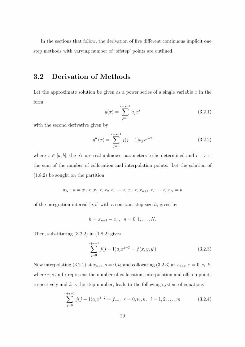
3.2 Derivation of Methods
Let the approximate solution be given as a power series of a single variable x in the
form
y(x) =r+s−1∑j=0
ajxj (3.2.1)
with the second derivative given by
y′′ (x) =r+s−1∑j=0
j(j − 1)ajxj−2 (3.2.2)
where x ∈ [a, b], the a’s are real unknown parameters to be determined and r + s is
the sum of the number of collocation and interpolation points. Let the solution of
(1.8.2) be sought on the partition
πN : a = x0 < x1 < x2 < · · · < xn < xn+1 < · · · < xN = b
of the integration interval [a, b] with a constant step size h, given by
h = xn+1 − xn, n = 0, 1, . . . , N.
Then, substituting (3.2.2) in (1.8.2) gives
r+s−1∑j=0
j(j − 1)ajxj−2 = f(x, y, y′) (3.2.3)
Now interpolating (3.2.1) at xn+s, s = 0, νi and collocating (3.2.3) at xn+r, r = 0, νi, k,
where r, s and i represent the number of collocation, interpolation and offstep points
respectively and k is the step number, leads to the following system of equations
r+s−1∑j=0
j(j − 1)ajxj−2 = fn+r, r = 0, νi, k, i = 1, 2, . . . ,m (3.2.4)
20

r+s−1∑j=0
ajxjn+s = yn+s, s = 0, νi, i = 1, . . . ,m (3.2.5)
(3.2.4) and (3.2.5) can be combined to form a matrix as follows
x0n x1n x2n x3n · · · xN
x0n+ν1 x1n+ν1 x2n+ν1 x3n+ν1 · · · xNn+ν1
......
......
......
x0n+νm x1n+νm x2n+νm x3n+νm · · · xNn+νm
0 0 2x0n 6x1n · · · N(N − 1)xN−2N
0 0 2x0n+ν1 6x1n+ν1 · · · N(N − 1)xN−2n+ν1
......
......
......
0 0 2x0n+νm 6x1n+νm · · · N(N − 1)xN−2n+νm
0 0 2x0n+1 6x1n+1 · · · N(N − 1)xN−2n+1
a0
a1..................
ar+s−1
=
yn
yn+ν1...
yn+νm
fn
fn+ν1...
fn+νm
fn+1
(3.2.6)
where νi ∈ (x0, xn+1), i = 1, · · · ,m.
Using Gaussian elimination method, (3.2.6) is solved for the aj’s. The values of the
aj’s obtained are then substituted into (3.2.1) to give, after some manipulations, a
continuous hybrid one step method in the form of the continuous linear multistep
method
y(x) =k∑j=0
αj(x)yn+j +∑νi
ανi(x)yn+νi + h2
[k∑j=0
βj(x)fn+j +∑νi
βνi(x)fn+νi
],
(3.2.7)
where yn+j = y(xn+j) and fn+j = f(xn+j, yn+j, y′n+j) and µ, is the order of the
problem.
In what follows, let us express αj(x) and βj(x) as continuous functions of t by
letting
t =x− xn+νi
h(3.2.8)
21
and noting that
dt
dx=
1
h.
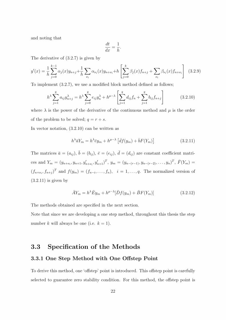
The derivative of (3.2.7) is given by
y′(x) =1
h
k−1∑j=0
αj(x)yn+j+1
h
∑νi
ανi(x)yn+νi+h
[k∑j=0
βj(x)fn+j +∑νi
βνi(x)fn+νi
](3.2.9)
To implement (3.2.7), we use a modified block method defined as follows;
hλq∑j=1
aijyλn+j = hλ
q∑j=0
eijyλn + hµ−λ
[q∑j=1
dijfn +
q∑j=1
bijfn+j
](3.2.10)
where λ is the power of the derivative of the continuous method and µ is the order
of the problem to be solved; q = r + s.
In vector notation, (3.2.10) can be written as
hλaYm = hλeym + hµ−λ[df(ym) + bF (Ym)
](3.2.11)
The matrices a = (aij), b = (bij), e = (eij), d = (dij) are constant coefficient matri-
ces and Ym = (yn+νi , yn+1, y′n+νi
, y′n+1)T , ym = (yn−(r−1), yn−(r−2), . . . , yn)T , F (Ym) =
(fn+νi , fn+j)T and f(ym) = (fn−i, . . . , fn), i = 1, . . . , q. The normalized version of
(3.2.11) is given by
AYm = hλEym + hµ−λ[Df(ym) + BF (Ym)] (3.2.12)
The methods obtained are specified in the next section.
Note that since we are developing a one step method, throughout this thesis the step
number k will always be one (i.e. k = 1).
3.3 Specification of the Methods
3.3.1 One Step Method with One Offstep Point
To derive this method, one ‘offstep’ point is introduced. This offstep point is carefully
selected to guarantee zero stability condition. For this method, the offstep point is
22

ν1 = 12. Using (3.2.1) with r = 3 and s = 2, we have a polynomial of degree r+ s− 1
as follows:
y(x) =4∑j=0
ajxj (3.3.1)
with second derivative given by
y′′(x) =4∑j=0
j(j − 1)ajxj−2 (3.3.2)
Substituting (3.3.2) into (1.8.2) gives
4∑j=0
j(j − 1)ajxj−2 = f(x, y, y′) (3.3.3)
Now collocating (3.3.3) at xn+r, r = 0, 12
and 1, and interpolating (3.3.1) at xn+s, s =
0, 12
leads to a system of equations written in the matrix form AX = B as
1 xn x2n x3n x4n
1 xn+ 12
x2n+ 1
2
x3n+ 1
2
x4n+ 1
2
0 0 2 6xn 12x2n
0 0 2 6xn+ 12
12x2n+ 1
2
0 0 2 6xn+1 12x2n+1
a0
a1
a2
a3
a4
=
yn
yn+ 12
fn
fn+ 12
fn+1
(3.3.4)
Equation (3.3.4) is solved by Gaussian elimination method to obtain the value of the
unknown parameters aj, (j = 0, 1, · · · , 4) as follows:
a0 = yn − a1xn − a2x2n − a3x3n − a4x4
a1 =yn+ 1
2− yn
12h
− a2(xn+ 12− xn)− a3(x2n+ 1
2+ xn+ 1
2xn + x2n)
a2 =1
2fn − 3a3xn − 6a4x
2n
a3 =fn+ 1
2
3h− 2a4(xn+ 1
2+ xn)
a4 =
12fn1 − fn+ 1
2+ 1
2fn
3h2
(3.3.5)
23

Substituting (3.3.5) into (3.3.1) yields a continuous implicit hybrid one step method
in the form of a continuous linear multistep method described by the formula
y(x) =k∑j=0
αj(x)yn+j+∑νi
ανi(x)yn+νi +h2
[k∑j=0
βj(x)fn+j +∑νi
βνi(x)yn+νi
](3.3.6)
where, for k = 1, i = 1 and ν1 = 12, yields the parameters αj and βj, j = 0, ν1, 1 as
the following continuous functions of t
α0(t) = −2t
α 12(t) = 2t+ 1
β0(t) =h2
48(8t4 − 8t3 + 3t)
β 12(t) =
h2
24(−8t4 + 12t2 + 5t)
β1(t) =h2
48(8t4 + 8t3 − t)
(3.3.7)
Using (3.3.7) for x = xn+1 and i = 1 so that t = 12, (3.3.6) reduces to
yn+1 − 2yn+ 12
+ yn =h2
48
[fn+1 + 10fn+ 1
2+ fn
](3.3.8)
Differentiating (3.3.7) yields
α′0(t) =−2
h
α′12(t) =
2
h
β′0(t) =h
48(32t3 − 24t2 + 3)
β′12(t) =
h
48(−32t3 + 24t+ 5)
β′1(t) =h
48(32t3 + 24t2 − 1)
(3.3.9)
24

On evaluating (3.3.9) at x = xn,xn+ 12
and xn+1 respectively, using (3.2.8) so that
t = −12, 0, 1
2, the following discrete methods are obtained
48hy′n − 96yn+ 12
+ 96yn = h2[fn+1 − 6fn+ 1
2− 7fn
]48hy′
n+ 12− 96yn+ 1
2+ 96yn = h2
[−fn+1 + 10fn+ 1
2+ 3fn
]48hy′n+1 − 96yn+ 1
2+ 96yn = h2
[9fn+1 + 26fn+ 1
2+ fn
](3.3.10)
The modified block formulae (3.2.11) and (3.2.12) are employed to simultaneously
obtain values for yn+ 12, yn+1, y
′n+ 1
2
and y′n+1 needed to implement (3.3.8). Now,
combining (3.3.8) and (3.3.10) in the form of (3.2.11) and (3.2.12) yield the block
method
−96 48 0 0
−96 0 0 0
−96 0 48h 0
−96 0 0 48h
yn+ 12
yn+1
y′n+ 1
2
y′n+1
=
−48 0
−96 48h
−96 0
−96 0
[yny′n
]+
h2
−7h2
3h2
h2
[fn]
+
10h2 h2
−6h2 h2
10h2 −h2
26h2 9h2
[fn+ 1
2
fn+1
](3.3.11)
Using (3.2.12), we obtain the block solution
1 0 0 0
0 1 0 0
0 0 1 0
0 0 0 1
yn+ 12
yn+1
y′n+ 1
2
y′n+1
=
10 12h
1 h
0 1
0 1
[yny′n
]+
796h2
16h2
524h
16h
[fn]
25
+
116h2 − 1
96h2
13h2 0
13h − 1
24h
23h 1
6h
[fn+ 1
2
fn+1
](3.3.12)
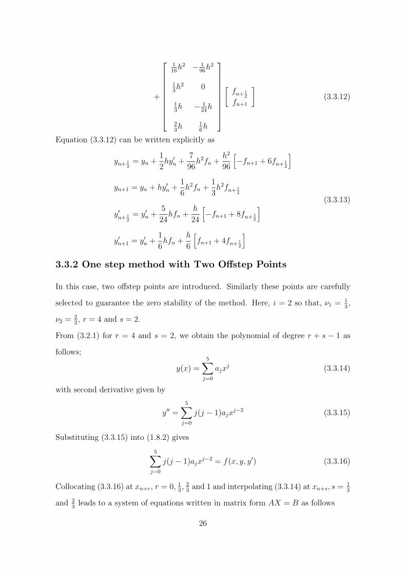
Equation (3.3.12) can be written explicitly as
yn+ 12
= yn +1
2hy′n +
7
96h2fn +
h2
96
[−fn+1 + 6fn+ 1
2
]yn+1 = yn + hy′n +
1
6h2fn +
1
3h2fn+ 1
2
y′n+ 1
2= y′n +
5
24hfn +
h
24
[−fn+1 + 8fn+ 1
2
]y′n+1 = y′n +
1
6hfn +
h
6
[fn+1 + 4fn+ 1
2
](3.3.13)
3.3.2 One step method with Two Offstep Points
In this case, two offstep points are introduced. Similarly these points are carefully
selected to guarantee the zero stability of the method. Here, i = 2 so that, ν1 = 13,
ν2 = 23, r = 4 and s = 2.
From (3.2.1) for r = 4 and s = 2, we obtain the polynomial of degree r + s − 1 as
follows;
y(x) =5∑j=0
ajxj (3.3.14)
with second derivative given by
y′′ =5∑j=0
j(j − 1)ajxj−2 (3.3.15)
Substituting (3.3.15) into (1.8.2) gives
5∑j=0
j(j − 1)ajxj−2 = f(x, y, y′) (3.3.16)
Collocating (3.3.16) at xn+r, r = 0, 13, 23
and 1 and interpolating (3.3.14) at xn+s, s = 13
and 23
leads to a system of equations written in matrix form AX = B as follows
26

1 xn+ 13
x2n+ 1
3
x3n+ 1
3
x4n+ 1
3
x5n+ 1
3
1 xn+ 23
x2n+ 2
3
x3n+ 2
3
x4n+ 2
3
x5n+ 2
3
0 0 2 6xn 12x2n 20x3n
0 0 2 6xn+ 13
12x2n+ 1
3
20x3n+ 1
3
0 0 2 6xn+ 23
12x2n+ 2
3
20x3n+ 2
3
0 0 2 6xn+1 12x2n+1 20x3n+1
a0
a1
a2
a3
a4
a5
=
yn+ 13
yn+ 23
fn
fn+ 13
fn+ 23
fn+1
(3.3.17)
Solving (3.3.17) by Gaussian elimination method yields the aj’s as follows
a0 = yn+ 13− a1xn+ 1
3− a2x2n+ 1
3− a3x3n+ 1
3− a4x4n+ 1
3− a5x5n+ 1
3
a1 =yn+ 2
3− yn+ 1
3
13h
− a2(xn+ 23
+ xn+ 13)− a3(x2n+ 2
3+ xn+ 2
3xn+ 1
3+ x2
n+ 13)
−a4(x3n+ 2
3+ x2
n+ 23xn+ 1
3+ xn+ 2
3x2n+ 1
3+ x3
n+ 13
)−a5
(x4n+ 2
3+ x3
n+ 23xn+ 1
3+ x2
n+ 23x2n+ 1
3+ xn+ 2
3x3n+ 2
3+ x4
n+ 13
)(3.3.18)
a2 =1
2fn − 3a3xn − 6a4x
2n − 10a5x
3n
a3 =fn+ 1
3− fn
2h− 2a4(xn+ 1
3+ xn)− 10
3a5
(x2n+ 1
3+ xn+ 1
3xn + x2n
)a4 =
13fn+ 2
3− 2
3fn+ 1
3+ 1
3fn
89h2
− 5
3a5
(xn+1 + xn+ 1
3+ xn
)a5 =
227fn+1 − 2
9fn+ 2
3+ 2
9fn+ 1
3− 2
27fn
80243h3
Substituting the ajs, j = 0(1)5 into (3.3.14) yields the continuous implicit hybrid one
step method in the form of a continuous linear multistep method described by the
formula
y(x) =k∑j=0
αj(x)yn+j+∑νi
ανiyn+νi+h2
[k∑j=0
βj(x)fn+j +∑νi
βνi(x)fn+νi
], i = 1, 2, (3.3.19)
27

For k = 1, ν1 = 13
and ν2 = 23
and writing the αj’s and βj’s as continuous functions
of t, where t =x−x
n+13
h, we obtain the parameters
α 13(t) = −3t
α 23(t) = 3t+ 1
β0(t) = − h2
1080(243t5 − 90t3 + 7t)
β 13(t) =
h2
360(243t5 + 135t4 − 180t3 + 22t)
β 23(t) = − h2
360(243t5 + 270t4 − 90t3 − 180t2 − 43t)
β1(t) =h2
1080(243t5 + 405t4 + 180t3 − 8t)
(3.3.20)
Evaluating (3.3.19) at x = xn and xn+1 using (3.2.8) gives values of t to be −23
and
13. Thus, we obtain the discrete methods from (3.3.20) as follows
yn+1 − 2yn+ 23
+ yn+ 13
=h2
108
[fn+1 + 10fn+ 2
3+ fn+ 1
3
](3.3.21a)
yn+ 23− 2yn+ 1
3+ yn =
h2
108
[fn+ 2
3+ 10fn+ 1
3+ fn
](3.3.21b)
Differentiating (3.3.20) gives
α′13
(t) = −3
h
α′23
(t) =3
h
β′0(t) = − h
1080(1215t4 − 270t2 + 7)
β′13
(t) =h
360(1215t5 + 540t3 − 540t2 + 22)
β′23
(t) = − h
360(1215t4 + 1080t3 − 270t2 − 360t− 43)
β′1(t) =h
1080(1215t4 + 1620t3 + 540t2 − 8)
(3.3.22)
28

Evaluating (3.3.22) at x = xn, xn+ 13, xn+ 2
3using (3.2.8) implies t = −2
3, −1
3, 0 and 1
3
Hence, the following discrete derivative methods are obtained.
1080hy′n − 3240yn+ 23
+ 3240yn+ 13
= h2[−8fn+1 + 9fn+ 2
3− 414fn+ 1
3− 127fn
]1080hy′
n+ 13− 3240yn+ 2
3+ 3240yn+ 1
3= h2
[7fn+1 − 66fn+ 2
3− 129fn+ 1
3+ 8fn
](3.3.23)
1080hy′n+ 2
3− 3240yn+ 2
3+ 3240yn+ 1
3= h2
[−8fn+1 + 129fn+ 2
3+ 66fn+ 1
3− 7fn
]1080hy′n+1 − 3240yn+ 2
3+ 3240yn+ 1
3= h2
[127fn+1 + 414fn+ 2
3− 9fn+ 2
3+ 8fn
]Combining (3.3.21) and (3.3.23) using the block formulae (3.2.11) and (3.2.12) we
have, respectively,
−216 108 0 0 0 0
108 −216 108 0 0 0
3240 −3240 0 0 0 0
3240 −3240 0 1080h 0 0
3240 −3240 0 0 1080h 0
3240 −3240 0 0 0 1080h
yn+ 13
yn+ 23
yn+1
y′n+ 1
3
y′n+ 2
3
y′n+1
=
108 0
0 0
0 1080h
0 0
0 0
0 0
yn
y′n
+
0
h2
−127h2
8h2
−7h2
8h2
[fn] +
h2 10h2 h2
10h2 h2 0
414h2 9h2 −8h2
−129h2 −66h2 7h2
66h2 129h2 −8h2
−9h2 414h2 127h2
fn+ 1
3
fn+ 23
fn+1
(3.3.24)
29
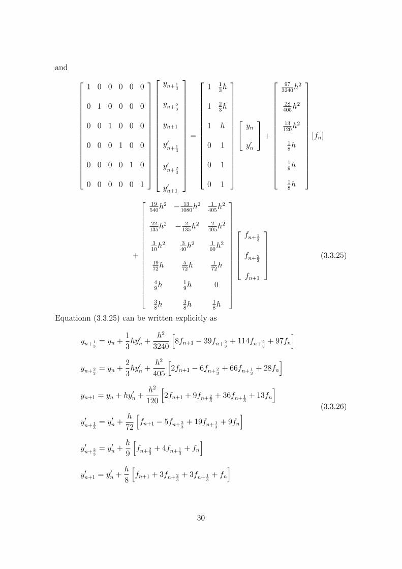
and
1 0 0 0 0 0
0 1 0 0 0 0
0 0 1 0 0 0
0 0 0 1 0 0
0 0 0 0 1 0
0 0 0 0 0 1
yn+ 13
yn+ 23
yn+1
y′n+ 1
3
y′n+ 2
3
y′n+1
=
1 13h
1 23h
1 h
0 1
0 1
0 1
yn
y′n
+
973240
h2
28405h2
13120h2
18h
19h
18h
[fn]
+
19540h2 − 13
1080h2 1
405h2
22135h2 − 2
135h2 2
405h2
310h2 3
40h2 1
60h2
1972h 5
72h 1
72h
49h 1
9h 0
38h 3
8h 1
8h
fn+ 1
3
fn+ 23
fn+1
(3.3.25)
Equationn (3.3.25) can be written explicitly as
yn+ 13
= yn +1
3hy′n +
h2
3240
[8fn+1 − 39fn+ 2
3+ 114fn+ 2
3+ 97fn
]yn+ 2
3= yn +
2
3hy′n +
h2
405
[2fn+1 − 6fn+ 2
3+ 66fn+ 1
3+ 28fn
]yn+1 = yn + hy′n +
h2
120
[2fn+1 + 9fn+ 2
3+ 36fn+ 1
3+ 13fn
]y′n+ 1
3= y′n +
h
72
[fn+1 − 5fn+ 2
3+ 19fn+ 1
3+ 9fn
]y′n+ 2
3= y′n +
h
9
[fn+ 2
3+ 4fn+ 1
3+ fn
]y′n+1 = y′n +
h
8
[fn+1 + 3fn+ 2
3+ 3fn+ 1
3+ fn
]
(3.3.26)
30
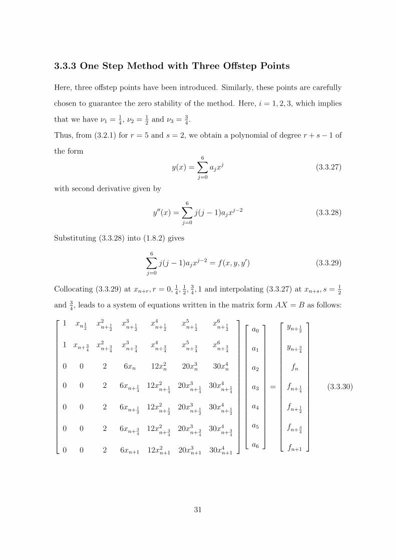
3.3.3 One Step Method with Three Offstep Points
Here, three offstep points have been introduced. Similarly, these points are carefully
chosen to guarantee the zero stability of the method. Here, i = 1, 2, 3, which implies
that we have ν1 = 14, ν2 = 1
2and ν3 = 3
4.
Thus, from (3.2.1) for r = 5 and s = 2, we obtain a polynomial of degree r+ s− 1 of
the form
y(x) =6∑j=0
ajxj (3.3.27)
with second derivative given by
y′′(x) =6∑j=0
j(j − 1)ajxj−2 (3.3.28)
Substituting (3.3.28) into (1.8.2) gives
6∑j=0
j(j − 1)ajxj−2 = f(x, y, y′) (3.3.29)
Collocating (3.3.29) at xn+r, r = 0, 14, 12, 34, 1 and interpolating (3.3.27) at xn+s, s = 1
2
and 34, leads to a system of equations written in the matrix form AX = B as follows:
1 xn 12
x2n+ 1
2
x3n+ 1
2
x4n+ 1
2
x5n+ 1
2
x6n+ 1
2
1 xn+ 34
x2n+ 3
4
x3n+ 3
4
x4n+ 3
4
x5n+ 3
4
x6n+ 3
4
0 0 2 6xn 12x2n 20x3n 30x4n
0 0 2 6xn+ 14
12x2n+ 1
4
20x3n+ 1
4
30x4n+ 1
4
0 0 2 6xn+ 12
12x2n+ 1
2
20x3n+ 1
2
30x4n+ 1
2
0 0 2 6xn+ 34
12x2n+ 3
4
20x3n+ 3
4
30x4n+ 3
4
0 0 2 6xn+1 12x2n+1 20x3n+1 30x4n+1
a0
a1
a2
a3
a4
a5
a6
=
yn+ 12
yn+ 34
fn
fn+ 14
fn+ 12
fn+ 34
fn+1
(3.3.30)
31

Solving (3.3.30) by Gaussian elimination yield the aj’s as follows:
a0 = yn+ 12− a1xn+ 1
2− a2x2n+ 1
2− a3x3n+ 1
2− a4x4n+ 1
2− a5x5n+ 1
2− a6x6n+ 1
2
a1 =yn+ 3
4− yn+ 1
2
14h
− a2(xn+ 3
4+ xn+ 1
2
)− a3
(x2n+ 3
4+ xn+ 3
4xn+ 1
2+ x2
n+ 11
)−a4
(x3n+ 3
4+ x2
n+ 34xn+ 1
2+ xn+ 3
4x2n+ 1
2+ x3
n+ 12
)− a5
(x4n+ 3
4+ x3
n+ 34xn+ 1
2
+x2n+ 3
4x2n+ 1
2+ xn+ 3
4x3n+ 1
2+ x4
n+ 12
)− a6
(x5n+ 3
4+ x4
n+ 34xn+ 1
2+ x3
n+ 34x2n+ 1
2
+x2n+ 3
4x3n+ 1
2+ xn+ 3
4x4n+ 1
2+ x5
n+ 12
)a2 =
1
2fn − 3a3xn − 6a4x
2n − 10x3n − 15x4n
a3 =fn+ 1
4− fn
32h
− 2a4
(xn+ 1
4+ xn
)+
10
3a5
(x2n+ 1
4+ xn+ 1
4xn + x2n
)−5a6
(x3n+ 1
4+ x2
n+ 14xn + xn+ 1
4x2n + x3n
)(3.3.31)
a4 =
14fn+ 1
2− 1
2fn+ 1
4+ 1
4fn
38h2
− 5
3a5
(xn+ 1
2+ xn+ 1
4+ xn
)−5
2a6
(x2n+ 1
2+ xn+ 1
2xn+ 1
4+ x2
n+ 14
+ xn+ 12xn + xn+ 1
4xn + x2n
)a5 =
132fn+ 3
4− 3
32fn+ 1
2+ 3
32fn+ 1
4− 1
32fn
15256h3
− 3
2a6
(xn+ 3
4+ xn+ 1
2+ xn+ 1
4+ xn
)a6 =
31024
fn+1 − 3256fn+ 3
4+ 9
512fn+ 1
2− 3
256fn+ 1
4+ 3
1024fn
13516384
h4
Substituting (3.3.31) into (3.3.27) yields the continuous implicit hybrid one step
method in the form of a continuous linear multistep method described by the for-
mula
y(x) =k∑j=0
αj(x)yn+j+∑νi
ανi(x)yn+νi+h2
[k∑j=0
βj(x)fn+j +∑νi
βνi(x)fn+νi
], i = 1, 2, 3 (3.3.32)
32
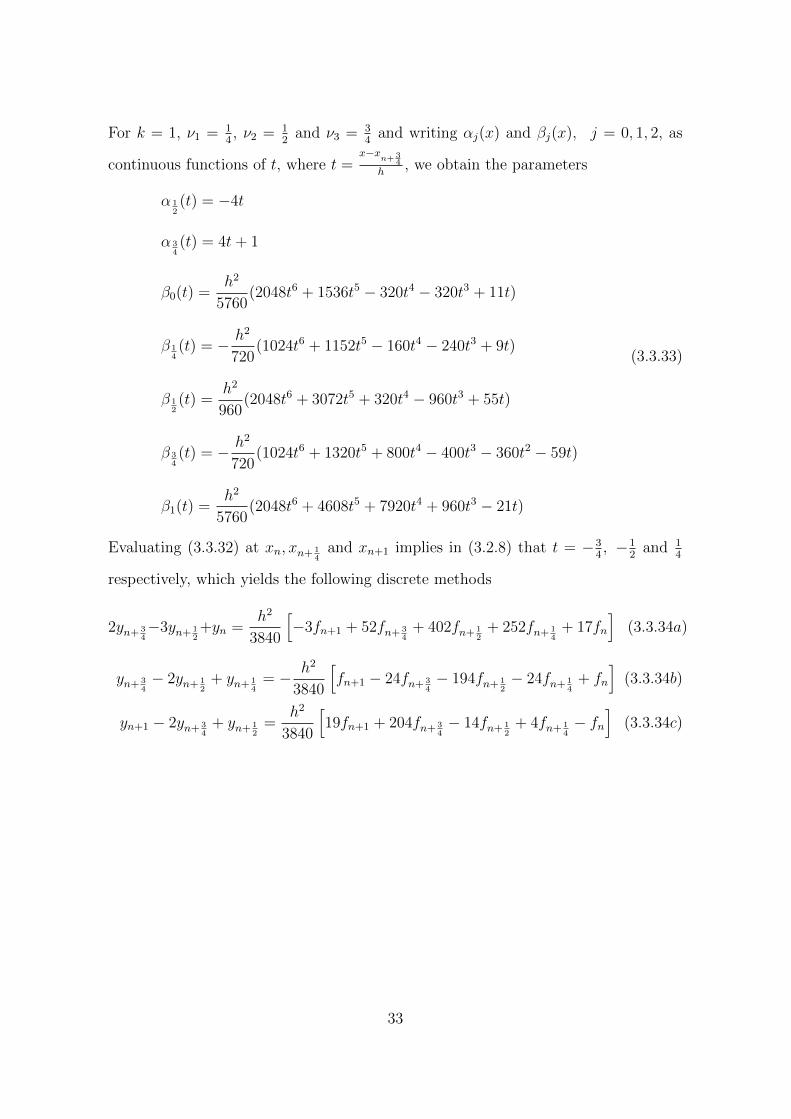
For k = 1, ν1 = 14, ν2 = 1
2and ν3 = 3
4and writing αj(x) and βj(x), j = 0, 1, 2, as
continuous functions of t, where t =x−x
n+34
h, we obtain the parameters
α 12(t) = −4t
α 34(t) = 4t+ 1
β0(t) =h2
5760(2048t6 + 1536t5 − 320t4 − 320t3 + 11t)
β 14(t) = − h2
720(1024t6 + 1152t5 − 160t4 − 240t3 + 9t)
β 12(t) =
h2
960(2048t6 + 3072t5 + 320t4 − 960t3 + 55t)
β 34(t) = − h2
720(1024t6 + 1320t5 + 800t4 − 400t3 − 360t2 − 59t)
β1(t) =h2
5760(2048t6 + 4608t5 + 7920t4 + 960t3 − 21t)
(3.3.33)
Evaluating (3.3.32) at xn, xn+ 14
and xn+1 implies in (3.2.8) that t = −34, −1
2and 1
4
respectively, which yields the following discrete methods
2yn+ 34−3yn+ 1
2+yn =
h2
3840
[−3fn+1 + 52fn+ 3
4+ 402fn+ 1
2+ 252fn+ 1
4+ 17fn
](3.3.34a)
yn+ 34− 2yn+ 1
2+ yn+ 1
4= − h2
3840
[fn+1 − 24fn+ 3
4− 194fn+ 1
2− 24fn+ 1
4+ fn
](3.3.34b)
yn+1 − 2yn+ 34
+ yn+ 12
=h2
3840
[19fn+1 + 204fn+ 3
4− 14fn+ 1
2+ 4fn+ 1
4− fn
](3.3.34c)
33

Differentiating (3.3.33) gives
α′12(t) =
−4
h
α′34(t) =
4
h
β′0(t) =h
5760(12288t5 + 7680t4 − 1280t3 − 960t2 + 11)
β′14(t) = − h
720(6144t5 − 5760t4 − 640t3 − 720t2 + 9)
β′12(t) =
h
960(12288t5 + 15360t4 + 1280t3 − 2880t2 + 55)
β′34(t) = − h
720(6144t5 + 11520t4 + 3200t3 − 1200t2 − 720t− 59)
β′1(t) =h
5760(12288t5 + 23040t4 + 14080t3 + 2880t2 − 21)
(3.3.35)
Evaluating (3.3.35) for t = −34,−1
2,−1
4, 0, 1
4, respectively, yields the following discrete
derivative methods
hy′n − 4yn+ 34
+ 4yn+ 12
=h2
5760
[33fn+1 − 284fn+ 3
4− 966fn+ 1
2− 1908fn+ 1
4− 475fn
]hy′
n+ 14− 4yn+ 3
4+ 4yn+ 1
2=
h2
5760
[−5fn+1 − 72fn+ 3
4− 1494fn+ 1
2− 616fn+ 1
4+ 27fn
]hy′
n+ 12− 4yn+ 3
4+ 4yn+ 1
2=
h2
5760
[17fn+1 − 220fn+ 3
4− 582fn+ 1
2+ 76fn+ 1
4− 11fn
](3.3.36)
hy′n+ 3
4− 4yn+ 3
4+ 4yn+ 1
2=
h2
5760
[−21fn+1 + 472fn+ 3
4+ 330fn+ 1
2− 72fn+ 1
4+ 11fn
]hy′n+1 − 4yn+ 3
4+ 4yn+ 1
2=
h2
5760
[481fn+1 + 1764fn+ 3
4− 198fn+ 1
2+ 140fn+ 1
4− 27fn
]
34

Combining (3.3.34) and (3.3.36), and using the modified block formulae (3.2.11) and
(3.2.12) respectively, we have
0 −11520 7680 0 0 0 0 0
3840 −7680 3840 0 0 0 0 0
0 3840 −7680 3840 0 0 0 0
0 23040 −23040 0 0 0 0 0
0 23040 −23040 0 5760h0 0 0 0
0 23040 −23040 0 0 5760h 0 0
0 23040 −23040 0 0 0 5760h 0
0 23040 −23040 0 0 0 0 5760h
yn+ 14
yn+ 12
yn+ 34
yn+1
y′n+ 1
4
y′n+ 1
2
y′n+ 3
4
y′n+1
=
−3840 0
0 0
0 0
0 −5760h
0 0
0 0
0 0
0 0
yn
y′n
+
17h2
−h2
−h2
−475h2
27h2
−11h2
11h2
−27h2
[fn]
35

+
252h2 402h2 52h2 −3h2
24h2 194h2 24h2 −h2
4h2 204h2 204h2 19h2
1908h2 −966h2 −284h2 33h2
−616h2 −1494h2 −72h2 −5h2
76h2 −582h2 −220h2 17h2
−72h2 330h2 472h2 −21h2
140h2 −198h2 1764h2 481h2
fn+ 14
fn+ 12
fn+ 34
yn+1
(3.3.37)
and
1 0 0 0 0 0 0 0
0 1 0 0 0 0 0 0
0 0 1 0 0 0 0 0
0 0 0 1 0 0 0 0
0 0 0 0 1 0 0 0
0 0 0 0 0 1 0 0
0 0 0 0 0 0 1 0
0 0 0 0 0 0 0 1
yn+ 14
yn+ 12
yn+ 34
yn+1
y′n+ 1
4
y′n+ 1
2
y′n+ 3
4
y′n+1
=
1 14h
1 12h
1 34h
1 h
0 1
0 1
0 1
0 1
yn
y′n
+
36723040
h2
531440
h2
1472560
h2
790h2
2512880
h
29360h
27320h
790h
[fn]
36

+
3128h2 − 47
3840h2 29
5760h2 − 7
7880h2
110h2 − 1
48h2 1
90h2 − 1
480h2
117640h2 27
1280h2 3
128h2 − 9
2560h2
415h2 1
15h2 4
45h2 0
3251440
h − 11120h 53
1440h − 19
2880h
3190h 1
5h 1
90h − 1
360h
51160h 9
40h 21
160h − 3
320h
1645h 2
15h 16
45h 7
90h
fn+ 14
fn+ 12
fn+ 34
fn+1
(3.3.38)
Equation (3.3.38) is written explicitly as
yn+ 14
= yn +1
4hy′n +
h2
23040
[−21fn+1 + 116fn+ 3
4− 282fn+ 1
2+ 540fn+ 1
4+ 367fn
]yn+ 1
2= yn +
1
2hy′n +
h2
1440
[−3fn+1 + 16fn+ 3
4− 30fn+ 1
2+ 144fn+ 1
4+ 53fn
]yn+ 3
4= yn +
3
4hy′n +
h2
2560
[−3fn+1 + 20fn+ 3
4+ 18fn+ 1
2+ 156fn+ 1
4+ 49fn
]yn+1 = yn + hy′n +
h2
90
[8fn+ 3
4+ 6fn+ 1
2+ 24fn+ 1
4+ 7fn
](3.3.39)
y′n+ 1
4= y′n +
h
2880
[−19fn+1 + 106fn+ 3
4− 264fn+ 1
2+ 646fn+ 1
4+ 251fn
]y′n+ 1
2= y′n +
h
360
[−fn+1 + 4fn+ 3
4+ 24fn+ 1
2+ 124fn+ 1
4+ 29fn
]y′n+ 3
4= y′n +
h
320
[−3fn+1 + 42fn+ 3
4+ 72fn+ 1
2+ 102fn+ 1
4+ 27fn
]y′n+1 = y′n +
h
90
[7fn+1 + 32fn+ 3
4+ 12fn+ 1
2+ 32fn+ 1
4+ 7fn
]
37

3.3.4 One Step Method with Four Offstep Points
Four offstep points have been introduced to derive this method. Like the previous
cases, the points are carefully chosen to guarantee the zero stability of the method.
Here, i = 1, 2, 3, 4, thus we have ν1 = 15, ν2 = 2
5, and ν3 = 3
5and ν4 = 4
5.
Thus, from (3.2.1) for r = 6 and s = 2 we obtain the basis polynomial of degree
r + s− 1 of the form
y(x) =7∑j=0
ajxj (3.3.40)
with second derivative given by
y′′ =7∑j=0
j(j − 1)ajxj−2 (3.3.41)
Substituting (3.3.41) into (1.8.2) gives the differential system
7∑j=0
j(j − 1)ajxj−2 = f(x, y, y′) (3.3.42)
Collocating (3.3.42) at xn+r, r = 0, 15, 25, 35, 45, 1 and interpolating (3.3.40) at xn+s, s =
35
and 45
leads to a system of equations written in the matrix form AX = B as follows
1 xn+ 35
x2n+ 3
5
x3n+ 3
5
x4n+ 3
5
x5n+ 3
5
x6n+ 3
5
x7n+ 3
5
1 xn+ 45
x2n+ 4
5
x3n+ 4
5
x4n+ 4
5
x5n+ 4
5
x6n+ 4
5
x7n+ 4
5
0 0 2 6xn 12x2n 20x3n 30x4n 42x5n
0 0 2 6xn+ 15
12x2n+ 1
5
20x3n+ 1
5
30x4n+ 1
5
42x5n+ 1
5
0 0 2 6xn+ 25
12x2n+ 2
5
20x3n+ 2
5
30x4n+ 2
5
42x5n+ 2
5
0 0 2 6xn+ 35
12x2n+ 3
5
20x3n+ 3
5
30x4n+ 3
5
42x5n+ 3
5
0 0 2 6xn+ 45
12x2n+ 4
5
20x3n+ 4
5
30x4n+ 4
5
42x5n+ 4
5
0 0 2 6xn+1 12x2n+1 20x3n+1 30x4n+1 42x4n+1
a0
a1
a2
a3
a4
a5
a6
a7
=
yn+ 35
yn+ 45
fn
fn+ 15
fn+ 25
fn+ 35
fn+ 45
fn+1
(3.3.43)
38

Solving (3.3.43) by Gaussian elimination method, the aj’s are obtained as follows
a0 = yn+ 35− a1xn+ 3
5− a2x2n+ 3
5− a3x3n+ 3
5− a4x4n+ 3
5− a5x5n+ 3
5− a6x6n+ 3
5− a7x7n+ 3
5
a1 =yn+ 4
5− yn+ 3
5
15h
− a2(xn+ 4
5+ xn+ 3
5
)− a3
(x2n+ 4
5+ xn+ 4
5xn+ 3
5+ x2
n+ 35
)−a4
(x3n+ 4
5+ x2
n+ 45xn+ 3
5+ xn+ 4
5x2n+ 3
5+ x3
n+ 35
)− a5
(x4n+ 4
5+ x3
n+ 45xn+ 4
5+ x2
n+ 45x2n+ 3
5
.+ xn+ 45x3n+ 3
5+ x4
n+ 35− a6
(x5n+ 4
5+ x4
n+ 45xn+ 3
5+ x3
n+ 45x2n+ 3
5+ x2
n+ 45x3n+ 3
5
+xn+ 45x4n+ 3
5+ x5
n+ 35
)− a7
(x6n+ 4
5+ x5
n+ 45xn+ 3
5+ x4
n+ 45x2n+ 3
5
+x3n+ 4
5x3n+ 3
5+ x2
n+ 45x4n+ 3
5+ xn+ 4
5x5n+ 3
5+ x6
n+ 35
)a2 =
1
2fn − 3a3xn − 6a4x
2n − 10a5x
3n − 15a6x
4n − 21a7x
5n
a3 =fn+ 1
5− fn
65h
− 2a4
(xn+ 1
5+ xn
)− 10
3a5
(x2n+ 1
5+ xn+ 1
5xn + x2n
)−5a6
(x3n+ 1
5+ x2
n+ 15xn + xn+ 1
5x2n + x3n
)− 7a7
(x4n+ 1
5+ x3
n+ 15xn + x2
n+ 15
+ xn+ 15x3n + x4n
)a4 =
15fn+ 2
5− 2
5fn+ 1
5+ 1
5fn
24125h2
− 5
3a5
(xn+ 2
5+ xn+ 1
5+ xn
)−5
2a6
(x2n+ 2
5+ xn+ 2
5xn+ 1
5+ x2
n+ 15
+ xn+ 25xn + xn+ 1
5xn + x2n
)−7
2a7
(x3n+ 2
5+ x2
n+ 25xn+ 1
5+ xn+ 2
5x2n+ 1
5+ x3
n+ 15
+ x2n+ 2
5xn + xn+ 2
5xn+ 1
5xn
+x2n+ 1
5xn + xn+ 2
5x2n + xn+ 1
5x2n + x3n
)(3.3.44)
a5 =
2125fn+ 3
5− 6
125fn+ 2
5+ 6
125fn+ 1
5− 2
125fn
483125
h3− 3
2a6
(xn+ 3
5+ xn+ 2
5+ xn+ 1
5+ xn
)−21
10a7
(x2n+ 3
5+ xn+ 3
5xn+ 2
5+ x2
n+ 25
+ xn+ 35xn+ 1
5+ xn+ 2
5xn+ 1
5+ x2
n+ 15
+ xn+ 35xn
+xn+ 25xn + xn+ 1
5xn + x2n
)a6 =
1215625
fn+ 45− 48
15625fn+ 3
5+ 72
15625fn+ 2
5− 48
15625fn+ 1
5+ 12
15625fn
17281943125
h4
−7
5a7
(xn+ 4
5+ xn+ 3
5+ xn+ 2
5+ xn+ 1
5+ xn
)a7 =
2889765625
fn+1 − 2881953125
fn+ 45
+ 5761953125
fn+ 35− 576
1953125fn+ 2
5+ 288
1953125fn+ 1
5− 288
9765625fn
2903046103515625
h5
39

Substituting (3.3.44) into (3.3.40) with some manipulation leads to the continuous
implicit hybrid one step method in the form of a CLMMs described by the formula
y(x) =k∑j=0
αj(x)yn+j+∑νi
ανi(x)yn+νi+h2
[k∑j=0
βj(x)fn+j +∑νi
βνi(x)fn+νi
], i = 1, 2, 3, 4 (3.3.45)
For k = 1, ν1 = 15,ν2 = 2
5,ν3 = 3
5,ν4 = 4
5and writing αj(x) and βj(x), j =
0, 15, 25, 35, 45, 1, as continuous functions of t, where t =
x−xn+4
5
h, we obtain the following
parameters
α 35(t) = −5t
α 45(t) = 5t+ 1
β0(t) =−h2
10080(6250t7 + 875t6 + 2625t5 − 875t4 − 420t3 + 8t)
β 15(t) =
h2
50400(156250t7 + 262500t6 + 91875t5 − 26250t4 − 14000t3 + 277t)
(3.3.46)
β 25(t) =
−h2
25200(156250t7 + 306250t6 + 144375t5 − 30625t4 − 21000t3 + 452t)
β 35(t) =
h2
5040(31250t7 + 70000t6 + 44625t5 − 1750t4 − 8400t3 + 271t)
β 45(t) =
−h2
50400(156250t7 + 393750t6 + 328125t5 + 65625t4 − 45500t3 − 25200t2 − 3104t)
β1(t) =h2
50400(31250t7 + 87500t6 + 91875t5 + 43750t4 + 8400t3 − 107t)
Evaluating (3.3.45) at xn, xn+ 15, xn+ 2
5and xn+1 and using (3.2.8) gives t = −4
5, −3
5,
−25, 15. Thus, from (3.3.46), the following discrete methods are obtained;
3yn+ 45−4yn+ 3
5+yn =
h2
3000
[−fn+1 + 32fn+ 4
5+ 322fn+ 3
5+ 232fn+ 2
5+ 127fn+ 1
5+ 8fn
](3.3.47a)
2yn+ 45−3yn+ 3
5+yn+ 1
5=−h2
6000
[2fn+1 − 47fn+ 4
5− 412fn+ 3
5− 242fn+ 2
5− 22fn+ 1
5+ fn
](3.3.47b)
yn+ 45−2yn+ 3
5+yn+ 2
5=−h2
6000
[fn+1 − 24fn+ 4
5− 194fn+ 3
5− 24fn+ 2
5+ fn+ 1
5
](3.3.47c)
yn+1−2yn+ 45+yn+ 3
5=
h2
6000
[18fn+1 + 209fn+ 4
5+ 4fn+ 3
5+ 14fn+ 2
5− 6fn+ 1
5+ fn
](3.3.47d)
40
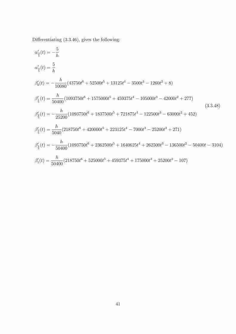
Differentiating (3.3.46), gives the following:
α′35(t) = −5
h
α′45(t) =
5
h
β′0(t) = − h
10080(43750t6 + 52500t5 + 13125t4 − 3500t3 − 1260t2 + 8)
β′15(t) =
h
50400(1093750t6 + 1575000t5 + 459375t4 − 105000t3 − 42000t2 + 277)
(3.3.48)
β′25(t) = − h
25200(1093750t6 + 1837500t5 + 721875t4 − 122500t3 − 63000t2 + 452)
β′35(t) =
h
5040(218750t6 + 420000t5 + 223125t4 − 7000t3 − 25200t2 + 271)
β′45(t) = − h
50400(1093750t6 + 2362500t5 + 1640625t4 + 262500t3 − 136500t2 − 50400t− 3104)
β′1(t) =h
50400(218750t6 + 525000t5 + 459375t4 + 175000t3 + 25200t2 − 107)
41
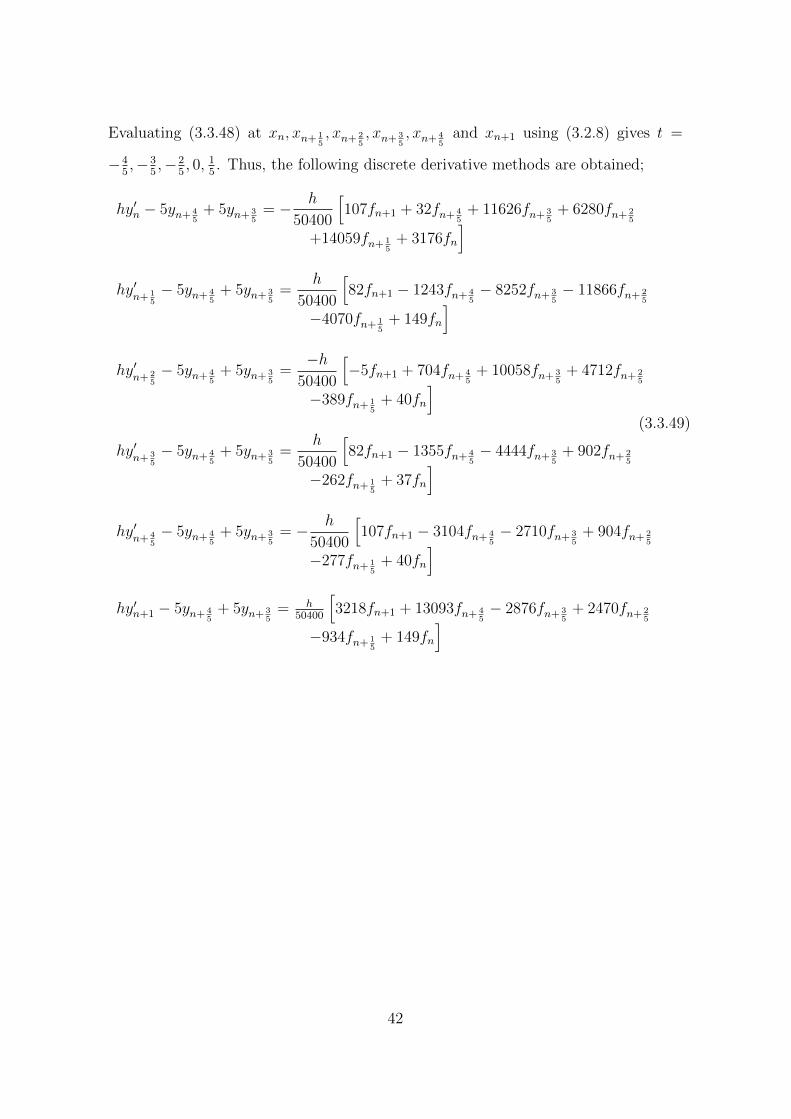
Evaluating (3.3.48) at xn, xn+ 15, xn+ 2
5, xn+ 3
5, xn+ 4
5and xn+1 using (3.2.8) gives t =
−45,−3
5,−2
5, 0, 1
5. Thus, the following discrete derivative methods are obtained;
hy′n − 5yn+ 45
+ 5yn+ 35
= − h
50400
[107fn+1 + 32fn+ 4
5+ 11626fn+ 3
5+ 6280fn+ 2
5
+14059fn+ 15
+ 3176fn
]hy′
n+ 15− 5yn+ 4
5+ 5yn+ 3
5=
h
50400
[82fn+1 − 1243fn+ 4
5− 8252fn+ 3
5− 11866fn+ 2
5
−4070fn+ 15
+ 149fn
]hy′
n+ 25− 5yn+ 4
5+ 5yn+ 3
5=−h
50400
[−5fn+1 + 704fn+ 4
5+ 10058fn+ 3
5+ 4712fn+ 2
5
−389fn+ 15
+ 40fn
](3.3.49)
hy′n+ 3
5− 5yn+ 4
5+ 5yn+ 3
5=
h
50400
[82fn+1 − 1355fn+ 4
5− 4444fn+ 3
5+ 902fn+ 2
5
−262fn+ 15
+ 37fn
]hy′
n+ 45− 5yn+ 4
5+ 5yn+ 3
5= − h
50400
[107fn+1 − 3104fn+ 4
5− 2710fn+ 3
5+ 904fn+ 2
5
−277fn+ 15
+ 40fn
]hy′n+1 − 5yn+ 4
5+ 5yn+ 3
5= h
50400
[3218fn+1 + 13093fn+ 4
5− 2876fn+ 3
5+ 2470fn+ 2
5
−934fn+ 15
+ 149fn
]
42

Combining (3.3.47) and (3.3.49) using (3.2.11) and (3.2.12) respectively gives
0 0 −12000 9000 0 0 0 0 0 0
6000 0 −18000 12000 0 0 0 0 0 0
0 6000 −12000 6000 0 0 0 0 0 0
0 0 6000 −12000 6000 0 0 0 0 0
0 0 252000 −252000 0 0 0 0 0 0
0 0 252000 −252000 0 50400h 0 0 0 0
0 0 252000 −252000 0 0 50400h 0 0 0
0 0 252000 −25200 0 0 0 50400h 0 0
0 0 25200 −252000 0 0 0 0 50400h 0
0 0 252000 −252000 0 0 0 0 0 50400h
yn+ 15
yn+ 25
yn+ 35
yn+ 45
yn+1
y′n+ 1
5
y′n+ 2
5
y′n+ 3
5
y′n+ 4
5
y′n+1
=
−3000 0
0 0
0 0
0 0
0 −50400h
0 0
0 0
0 0
0 0
0 0
yn
y′n
+
8h2
−h2
0
h2
−3176h2
149h2
−40h2
37h2
−40h2
149h2
[fn]
43

+
127h2 232h2 322h2 32h2 −h2
22h2 242h2 412h2 47h2 −2h2
24h2 24h2 194h2 24h2 −h2
−6h2 14h2 4h2 209h2 18h2
−14059h2 −6280h2 −11626h2 −32h2 −107h2
−4070h2 −11866h2 −8252h2 −1243h2 82h2
389h2 −4712h2 −10058h2 −704h2 5h2
−262h2 902h2 −4444h2 −1355h2 82h2
277h2 −904h2 2710h2 3104h2 −107h2
−934h2 2470h2 −2876h2 13093h2 3218h2
fn+ 15
fn+ 25
fn+ 35
fn+ 45
fn+1
(3.3.50)
and simplify to obtain
1 0 0 0 0 0 0 0 0 0
0 1 0 0 0 0 0 0 0 0
0 0 1 0 0 0 0 0 0 0
0 0 0 1 0 0 0 0 0 0
0 0 0 0 1 0 0 0 0 0
0 0 0 0 0 1 0 0 0 0
0 0 0 0 0 0 1 0 0 0
0 0 0 0 0 0 0 1 0 0
0 0 0 0 0 0 0 0 1 0
0 0 0 0 0 0 0 0 0 1
yn+ 15
yn+ 25
yn+ 35
yn+ 45
yn+1
y′n+ 1
5
y′n+ 2
5
y′n+ 3
5
y′n+ 4
5
y′n+1
=
1 15h
1 25h
1 35h
1 45h
1 h
0 1
0 1
0 1
0 1
0 1
yn
y′n
+
123112600
713150
1233500
3767875
611008
19288
14225
51800
14225
19288
[fn]
44
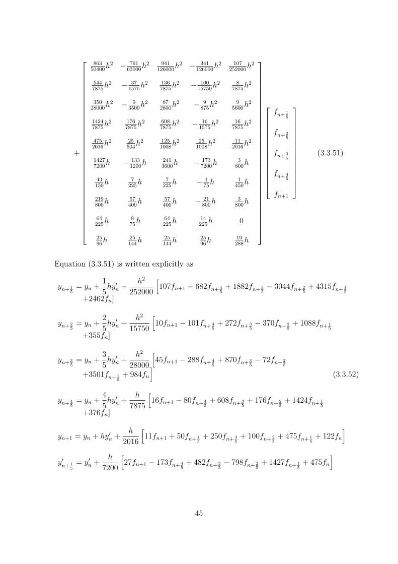
+
86350400
h2 − 76163000
h2 941126000
h2 − 341126000
h2 107252000
h2
5447875
h2 − 371575
h2 1367875
h2 − 10015750
h2 87875
h2
35028000
h2 − 93500
h2 872800
h2 − 9875h2 9
5600h2
14247875
h2 1767875
h2 6087875
h2 − 161575
h2 167875
h2
4752016
h2 25504h2 125
1008h2 25
1008h2 11
2016h2
14277200
h − 1331200
h 2413600
h − 1737200
h 3800h
43150h 7
225h 7
225h − 1
75h 1
450h
219800h 57
400h 57
400h − 21
800h 3
800h
64225h 8
75h 64
225h 14
225h 0
2596h 25
144h 25
144h 25
96h 19
288h
fn+ 15
fn+ 25
fn+ 35
fn+ 45
fn+1
(3.3.51)
Equation (3.3.51) is written explicitly as
yn+ 15
= yn +1
5hy′n +
h2
252000
[107fn+1 − 682fn+ 4
5+ 1882fn+ 3
5− 3044fn+ 2
5+ 4315fn+ 1
5
+2462fn]
yn+ 25
= yn +2
5hy′n +
h2
15750
[10fn+1 − 101fn+ 4
5+ 272fn+ 3
5− 370fn+ 2
5+ 1088fn+ 1
5
+355fn]
yn+ 35
= yn +3
5hy′n +
h2
28000
[45fn+1 − 288fn+ 4
5+ 870fn+ 3
5− 72fn+ 2
5
+3501fn+ 15
+ 984fn
](3.3.52)
yn+ 45
= yn +4
5hy′n +
h
7875
[16fn+1 − 80fn+ 4
5+ 608fn+ 3
5+ 176fn+ 2
5+ 1424fn+ 1
5
+376fn]
yn+1 = yn + hy′n +h
2016
[11fn+1 + 50fn+ 4
5+ 250fn+ 3
5+ 100fn+ 2
5+ 475fn+ 1
5+ 122fn
]y′n+ 1
5= y′n +
h
7200
[27fn+1 − 173fn+ 4
5+ 482fn+ 3
5− 798fn+ 2
5+ 1427fn+ 1
5+ 475fn
]
45

y′n+ 2
5= y′n +
h
450
[fn+1 − 6fn+ 4
5+ 14fn+ 3
5+ 14fn+ 2
5+ 129fn+ 1
5+ 28fn
]y′n+ 3
5= y′n +
h
800
[3fn+1 − 21fn+ 4
5+ 114fn+ 3
5+ 114fn+ 2
5+ 219fn+ 1
5+ 51fn
]y′n+ 4
5= y′n +
h
225
[14fn+ 4
5+ 64fn+ 3
5+ 24fn+ 2
5+ 64fn+ 1
5+ 14fn
]y′n+1 = y′n +
h
288
[19fn+1 + 75fn+ 4
5+ 50fn+ 3
5+ 50fn+ 2
5+ 75fn+ 1
5+ 19fn
]3.3.5 One Step Method with Five Offstep Points
This method is derived by the addition of five offstep points between xn and xn+1.
The offstep points are chosen carefully to guarantee zero stability of the method. In
particular, i = 1, 2, 3, 4, 5 which implies that ν1 = 16, ν2 = 1
3, ν3 = 1
2, ν4 = 2
3and
ν5 = 56.
Thus, (3.2.1) for r = 7 and s = 2 becomes a polynomial of degree r + s − 1 of the
form
y(x) =8∑j=0
ajxj (3.3.53)
with second derivative given by
y′′ =8∑j=0
j(j − 1)ajxj−2 (3.3.54)
Substituting (3.3.54) into (1.8.2) gives the differential system
8∑j=0
j(j − 1)ajxj−2 = f(x, y, y′) (3.3.55)
46

Collocating (3.3.55) at xn+r, r = 0, 16, 13, 12, 23, 56, 1 and interpolating (3.3.53) at xn+s, s =
23, 56
leads to a system of equations written in the matrix form AX = B as follows:
1 xn+ 23
x2n+ 2
3
x3n+ 2
3
x4n+ 2
3
x5n+ 2
3
x6n+ 2
3
x7n+ 2
3
x8n+ 2
3
1 xn+ 56
x2n+ 5
6
x3n+ 5
6
x4n+ 5
6
x5n+ 5
6
x6n+ 5
6
x7n+ 5
6
x8n+ 5
6
0 0 2 6xn 12x2n 20x3n 30x4n 42x5n 56x6n
0 0 2 6xn+ 16
12x2n+ 1
6
20x3n+ 1
6
30x4n+ 1
6
42x5n+ 1
6
56x6n+ 1
6
0 0 2 6xn+ 13
12x2n+ 1
3
20x3n+ 1
3
30x4n+ 1
3
42x5n+ 1
3
56x6n+ 1
3
0 0 2 6xn+ 12
12x2n+ 1
2
20x3n+ 1
2
30x4n+ 1
2
42x5n+ 1
2
56x6n+ 1
2
0 0 2 6xn+ 23
12x2n+ 2
3
20x3n+ 2
3
30x4n+ 2
3
42x5n+ 2
3
56x6n+ 2
3
0 0 2 6xn+ 56
12x2n+ 5
6
20x3n+ 5
6
30x4n+ 5
6
42x5n+ 5
6
56x6n+ 5
6
0 0 2 6xn+1 12x2n+1 20x3n+1 30x4n+1 42x5n+1 56x6n+1
a0
a1
a2
a3
a4
a5
a6
a7
a8
=
yn+ 23
yn+ 56
fn
fn+ 16
fn+ 13
fn+ 12
fn+ 23
fn+ 56
fn+1
(3.3.56)
47

Solving (3.3.56) by Gaussian elimination method, the following parameters were ob-
tained:
a0 = yn+ 23− a1xn+ 2
3− a2x2n+ 2
3− a3x3n+ 2
3− a4x4n+ 2
3− a5x5n+ 2
3− a6x6n+ 2
3− a7x7n+ 2
3− a8x8n+ 2
3
a1 =yn+ 5
6− yn+ 2
3
16h
− a2(xn+ 5
6+ xn+ 2
3
)− a3
(x2n+ 5
6+ xn+ 5
6xn+ 2
3+ x2
n+ 23
)−a4
(x3n+ 5
6+ x2
n+ 56xn+ 2
3+ xn+ 5
6x2n+ 2
3+ x3
n+ 23
)−a5
(x4n+ 5
6+ x3
n+ 56xn+ 2
3+ x2
n+ 56x2n+ 2
3+ xn+ 5
6x3n+ 2
3+ x4
n+ 23
)−a6
(x5n+ 5
6+ x4
n+ 56xn+ 2
3+ x3
n+ 56x2n+ 2
3+ x2
n+ 56x3n+ 2
3+xn+ 5
6x4n+ 2
3+ x5
n+ 23
)−a7
(x6n+ 5
6+ x5
n+ 56xn+ 2
3+ x4
n+ 56x2n+ 2
3+ x3
n+ 56x3n+ 2
3+ x2
n+ 56x4n+ 2
3+ xn+ 5
6x5n+ 2
3+ x6
n+ 23
)−a8
(x7n+ 5
6+ x6
n+ 56xn+ 2
3+ x5
n+ 56x2n+ 2
3+ x4
n+ 56x3n+ 2
3+ x3
n+ 56x4n+ 2
3
+x2n+ 5
6x5n+ 2
3+ xn+ 5
6x6n+ 2
3+ x7
n+ 23
)a2 =
1
2fn − 3a3xn − 6a4x
2n − 10a5x
3n − 15a6x
4n + 21a7x
5n + 28a8x
6n
a3 =fn+ 1
6− fnh
− 2a4
(xn+ 1
6+ xn
)− 10
3a5
(x2n+ 1
6+ xn+ 1
6xn + x2n
)−5a6
(x3n+ 1
6+ x2
n+ 16xn + xn+ 1
6x2n + x3n
)− 7a7
(x4n+ 1
6+ x3
n+ 16xn + x2
n+ 16x2n + xn+ 1
6x3n + x4n
)−28
3a8
(x5n+ 1
6+ x4
n+ 16xn + x3
n+ 16x2n + x2
n+ 16x3n + xn+ 1
6x4n + x5n
)a4 =
16fn+ 1
3− 1
3fn+ 1
6+ 1
6fn
19h2
− 5
3a5
(xn+ 1
3+ xn+ 1
6+ xn
)(3.3.57)
−5
2a6
(x2n+ 1
3+ xn+ 1
3xn+ 1
6+ x2
n+ 16
+ xn+ 13xn + xn+ 1
6xn + x2n
)−7
2a7
(x3n+ 1
3+ x2
n+ 13xn+ 1
6+ xn+ 1
3x2n+ 1
6+ x3
n+ 16
+ x2n+ 1
3xn + xn+ 1
3xn+ 1
6xn
+x2n+ 1
6xn + xn+ 1
3x2n + xn+ 1
6x2n + x3n
)−14
3a8
(x4n+ 1
3+ x3
n+ 13xn+ 1
6+ x2
n+ 13x2n+ 1
6+ xn+ 1
3x3n+ 1
3+ x4
n+ 13
+ x3n+ 1
3xn + x2
n+ 13xn+ 1
6xn
+xn+ 13x2n+ 1
6xn + x3
n+ 16xn + x2
n+ 13x2n + xn+ 1
3xn+ 1
6x2n + x2
n+ 16x2n + xn+ 1
3x3n + xn+ 1
6x3n + x4n
)a5 =
1108fn+ 1
2− 1
36fn+ 1
3+ 1
36fn+ 1
6− 1
108fn
5972h3
− 3
2a6
(xn+ 1
2+ xn+ 1
3+ xn+ 1
6+ xn
)−21
10a7
(x2n+ 1
2+ xn+ 1
2xn+ 1
3+ x2
n+ 13
+ xn+ 12xn+ 1
6+ xn+ 1
3xn+ 1
6+ x2
n+ 16
+ xn+ 12xn + xn+ 1
3xn
+xn+ 16xn + x2n
)48
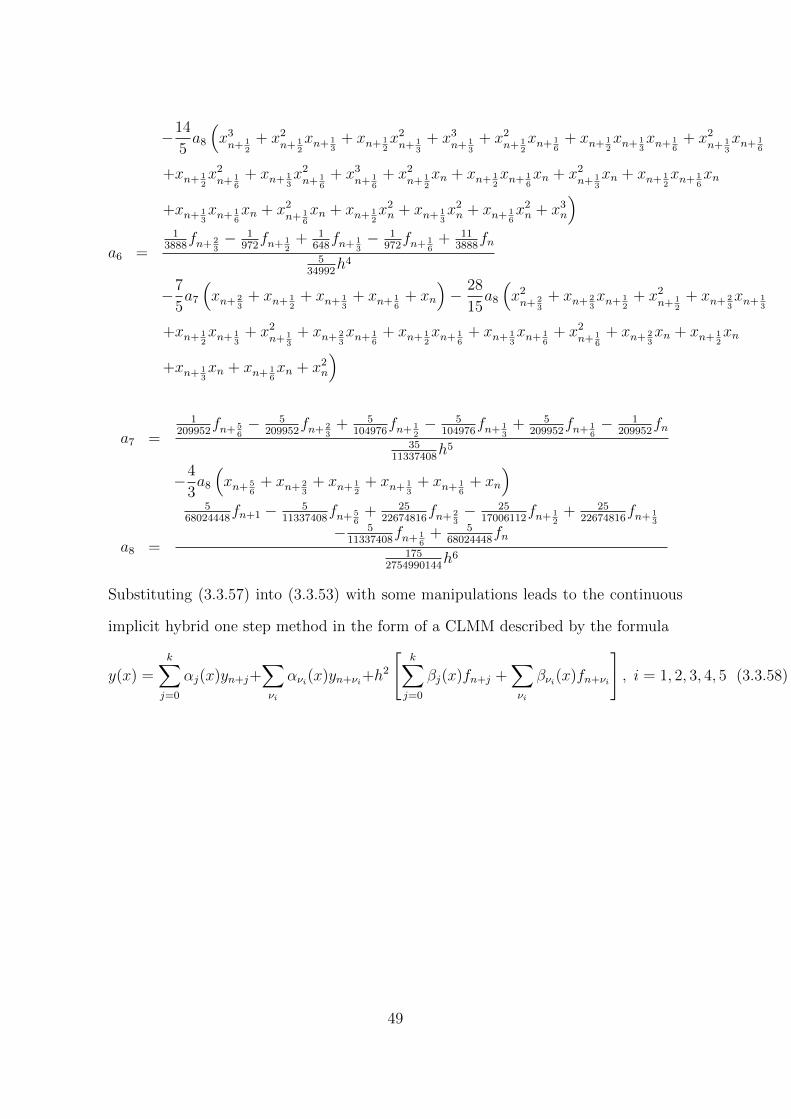
−14
5a8
(x3n+ 1
2+ x2
n+ 12xn+ 1
3+ xn+ 1
2x2n+ 1
3+ x3
n+ 13
+ x2n+ 1
2xn+ 1
6+ xn+ 1
2xn+ 1
3xn+ 1
6+ x2
n+ 13xn+ 1
6
+xn+ 12x2n+ 1
6+ xn+ 1
3x2n+ 1
6+ x3
n+ 16
+ x2n+ 1
2xn + xn+ 1
2xn+ 1
6xn + x2
n+ 13xn + xn+ 1
2xn+ 1
6xn
+xn+ 13xn+ 1
6xn + x2
n+ 16xn + xn+ 1
2x2n + xn+ 1
3x2n + xn+ 1
6x2n + x3n
)a6 =
13888
fn+ 23− 1
972fn+ 1
2+ 1
648fn+ 1
3− 1
972fn+ 1
6+ 11
3888fn
534992
h4
−7
5a7
(xn+ 2
3+ xn+ 1
2+ xn+ 1
3+ xn+ 1
6+ xn
)− 28
15a8
(x2n+ 2
3+ xn+ 2
3xn+ 1
2+ x2
n+ 12
+ xn+ 23xn+ 1
3
+xn+ 12xn+ 1
3+ x2
n+ 13
+ xn+ 23xn+ 1
6+ xn+ 1
2xn+ 1
6+ xn+ 1
3xn+ 1
6+ x2
n+ 16
+ xn+ 23xn + xn+ 1
2xn
+xn+ 13xn + xn+ 1
6xn + x2n
)
a7 =
1209952
fn+ 56− 5
209952fn+ 2
3+ 5
104976fn+ 1
2− 5
104976fn+ 1
3+ 5
209952fn+ 1
6− 1
209952fn
3511337408
h5
−4
3a8
(xn+ 5
6+ xn+ 2
3+ xn+ 1
2+ xn+ 1
3+ xn+ 1
6+ xn
)
a8 =
568024448
fn+1 − 511337408
fn+ 56
+ 2522674816
fn+ 23− 25
17006112fn+ 1
2+ 25
22674816fn+ 1
3
− 511337408
fn+ 16
+ 568024448
fn175
2754990144h6
Substituting (3.3.57) into (3.3.53) with some manipulations leads to the continuous
implicit hybrid one step method in the form of a CLMM described by the formula
y(x) =k∑j=0
αj(x)yn+j+∑νi
ανi(x)yn+νi+h2
[k∑j=0
βj(x)fn+j +∑νi
βνi(x)fn+νi
], i = 1, 2, 3, 4, 5 (3.3.58)
49

Now, for k = 1,ν1 = 16,ν2 = 1
3,ν3 = 1
2, ν4 = 2
3and ν5 = 5
6, let α(x) and β(x) be written
as continuous functions of t then, we obtain the following coefficients of (3.3.58) as:
α 35(t) = −6t
α 56(t) = 6t+ 1
β0(t) =h2
725760(839808t3 + 1679616t7 + 1088640t6 + 163296t5 − 78624t4 − 24192t3 + 289t)
β 16(t) =
−h2
13440(93312t8 + 207360t7 + 145152t6 + 24192t5 − 10416t4 − 3360t3 + 41t)
β 13(t) =
h2
80640(1399680t8 + 3421440t7 + 2685312t6 + 526176t5 − 191520t4 − 67200t3 + 851t)
β 12(t) = − h2
181440(4199040t8 + 11197440t7 + 10015488t6 + 2612736t5 − 710640t4
−302400t3 + 4157t) (3.3.59)
β 23(t) =
h2
8960(155520t8 + 449280t7 + 459648t6 + 167328t5 − 19040t4 − 22400t3 + 455t)
β 56(t) =
−h2
40320(279936t8 + 870912t7 + 1016064t6 + 508032t5 + 49392t4 − 51744t3
−20160t2 − 1973t)
β1(t) =h2
725760(839808t7 + 2799360t7 + 3701376t6 + 2449440t5 + 828576t4 + 120960t3 − 995t)
Evaluating (3.3.58) at xn, xn+ 16, xn+ 1
3, xn+ 1
2, xn+1 using (3.2.8) gives t = −5
6, −2
3,−1
2,−1
3, 16
and yields the following discrete methods from (3.3.59);
4yn+ 56−5yn+ 2
3+yn =
h2
217728
[−95fn+1 + 2334fn+ 5
6+ 21255fn+ 2
3+ 18532fn+ 1
2+ 11679fn+ 1
3
+6366n+ 16
+ 409fn
](3.3.60a)
3yn+ 56−4yn+ 5
6+yn+ 1
6= − h2
362880
[95fn+1 − 2754fn+ 5
6− 26883fn+ 2
3− 19708fn+ 1
2− 10503fn+ 1
3
−738fn+ 16
+ 11fn
](3.3.60b)
2yn+ 56− 3yn+ 2
3+ yn+ 1
3=
h2
725760
[−137fn+1 + 3762n+ 5
6+ 35073fn+ 2
3+ 19708fn+ 1
2+ 2313fn+ 1
3
50

−270fn+ 16
+ 31fn
](3.3.60c)
yn+ 56− 2yn+ 2
3+ yn+ 1
2=
h2
2177280
[−221fn+1 + 5862fn+ 5
6+ 49353fn+ 2
3+ 5428fn+ 1
2
+213fn+ 13− 186fn+ 1
6+ 31fn
](3.3.60d)
yn+1 − 2yn+ 56
+ yn+ 23
= − h2
2177280
[−4315fn+1 − 53994fn+ 5
6+ 2307fn+ 2
3− 7948fn+ 1
2
+4827fn+ 13− 1578fn+ 1
6+ 221fn
](3.3.60e)
Differentiating (3.3.59) yields the following:
α′23(t) = −6
h
α′56(t) =
6
h
β′0(t) =h
725760(6718464t7 + 11757312t6 + 6531840t5 + 816480t4 − 314496t3 − 7257t2 + 289)
β′16(t) = − h
13440(746469t7 + 1451520t6 + 870912t5 + 120960t4 − 41664t3 − 10080t2 + 41)
β′13(t) =
h
80640(11197440t7 + 23950080t6 + 16111872t5 + 2630880t4 − 766080t3
−201600t2 + 851)(3.3.61)
β′12(t) = − h
181440(33592320t7 + 78382080t6 + 60092928t5 + 13063680t4 − 2842560t3
−907200t2 + 4157)
β′23(t) =
h
40320(2239488t7 + 6096384t6 + 6096384t5 + 2540160t4 + 197568t3 − 155232t2
−40320t− 1973)
β′1(t) =h
725760(6718464t7 + 19595520t6 + 22208256t5 + 12247200t4 + 3314304t3
+362880t2 − 995)
51

Evaluating (3.3.61) for t = −56,−2
3,−1
2,−1
3,−1
6, 0 and 1
6the following derivative meth-
ods were obtained:
hy′n − 6yn+ 56
+ 6yn+ 23
= − h2
241920
[−585fn+1 + 6962fn+ 5
6+ 26465fn+ 2
3+ 58876fn+ 1
2
+18697fn+ 13
+ 58738fn+ 16
+ 12287fn
]hy′
n+ 16− 6yn+ 5
6+ 6yn+ 2
3=
h2
725760
[29fn+1 − 8262fn+ 5
6− 119817fn+ 2
3− 101620fn+ 1
2
−149013fn+ 13− 45990fn+ 1
6+ 1313fn
]hy′
n+ 13− 6yn+ 5
6+ 6yn+ 2
3=−h2
725760
[−571fn+1 + 12438fn+ 5
6+ 105219fn+ 2
3+ 134132fn+ 1
2
+55035fn+ 13− 4266fn+ 1
6+ 413fn
]hy′
n+ 12− 6yn+ 5
6+ 6yn+ 2
6=
h2
241920
[63fn+1 − 3074fn+ 5
6− 39587fn+ 2
3− 19708fn+ 1
2
+2201fn+ 13− 418fn+ 1
6+ 43fn
](3.3.62)
hy′n+ 2
3− 6yn+ 5
6+ 6yn+ 2
3= − h2
725760
[−731fn+1 + 14742fn+ 5
6+ 57123fn+ 2
3− 15884fn+ 1
2
+6939fn+ 13− 1962fn+ 1
6+ 253fn
]hy′
n+ 56− 6yn+ 5
6+ 6yn+ 2
3=
h2
725760
[−995fn+1 + 35514fn+ 5
6+ 36855fn+ 2
3− 16628fn+ 1
2
+7659fn+ 13− 2214fn+ 1
6+ 289fn
]hy′n+1 − 6yn+ 5
6+ 6yn+ 2
3= − h2
241920
[−12393fn+1 − 55246fn+ 5
6+ 18689fn+ 2
3− 19460fn+ 1
2
+10921fn+ 13− 3470fn+ 1
6+ 479fn
]Combining (3.3.60) and (3.3.62) using (3.1.11) and (3.2.12) respectively gives
52
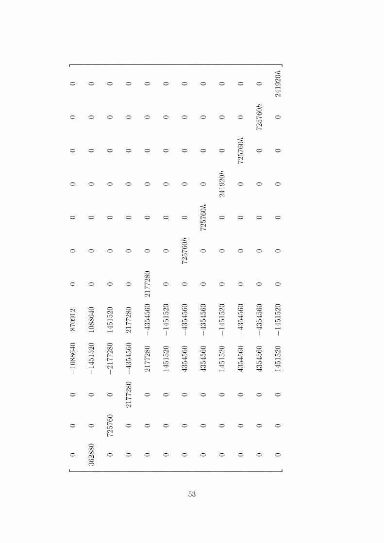
00
0−
1088
640
8709
120
00
00
00
3628
800
0−
1451
520
1088
640
00
00
00
0
072
5760
0−
2177
280
1451
520
00
00
00
0
00
2177
280−
4354
560
2177
280
00
00
00
0
00
021
7728
0−
4354
560
2177
280
00
00
00
00
014
5152
0−
1451
520
00
00
00
0
00
043
5456
0−
4354
560
072
5760h
00
00
0
00
043
5456
0−
4354
560
00
7257
60h
00
00
00
014
5152
0−
1451
520
00
024
1920h
00
0
00
043
5456
0−
4354
560
00
00
7257
60h
00
00
043
5456
0−
4354
560
00
00
072
5760h
0
00
014
5152
0−
1451
520
00
00
00
2419
20h
53
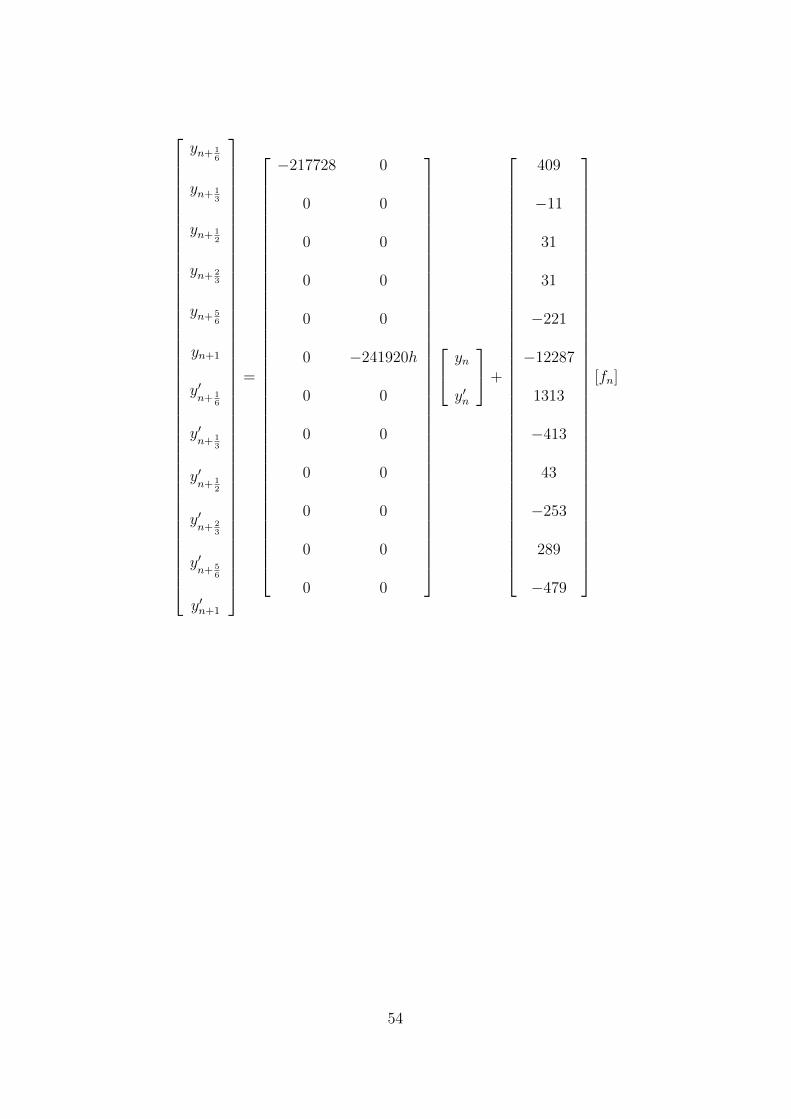
yn+ 16
yn+ 13
yn+ 12
yn+ 23
yn+ 56
yn+1
y′n+ 1
6
y′n+ 1
3
y′n+ 1
2
y′n+ 2
3
y′n+ 5
6
y′n+1
=
−217728 0
0 0
0 0
0 0
0 0
0 −241920h
0 0
0 0
0 0
0 0
0 0
0 0
yn
y′n
+
409
−11
31
31
−221
−12287
1313
−413
43
−253
289
−479
[fn]
54

+
6366h2 11679h2 18532h2 21255h2 2334h2 −95h2
738h2 10503h2 19708h2 26883h2 2754h2 95h2
−270h2 2313h2 19708h2 35073h2 3762h2 −137h2
−186h2 213h2 5428h2 49353h2 5862h2 −221h2
−1578h2 −4827h2 7948h2 −2307h2 53994h2 4315h2
−58738h2 −18697h2 −58876h2 −26465h2 −6962h2 585h2
−45990h2 −149013h2 −101620h2 −119817h2 −8262h2 29h2
4266h2 −55035h2 −134132h2 −105219h2 −12438h2 571h2
−418h2 2201h2 −19708h2 −39587h2 −3074h2 63h2
1962h2 −6939h2 15884h2 −57123h2 −14742h2 731h2
−2214h2 7659h2 −16628h2 36855h2 35514h2 −995h2
3470h2 −10921h2 19460h2 −18689h2 55246h2 12393h2
fn+ 16
fn+ 13
fn+ 12
fn+ 23
fn+ 56
fn+1
(3.3.63)
55
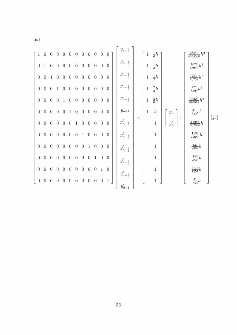
and
1 0 0 0 0 0 0 0 0 0 0 0
0 1 0 0 0 0 0 0 0 0 0 0
0 0 1 0 0 0 0 0 0 0 0 0
0 0 0 1 0 0 0 0 0 0 0 0
0 0 0 0 1 0 0 0 0 0 0 0
0 0 0 0 0 1 0 0 0 0 0 0
0 0 0 0 0 0 1 0 0 0 0 0
0 0 0 0 0 0 0 1 0 0 0 0
0 0 0 0 0 0 0 0 1 0 0 0
0 0 0 0 0 0 0 0 0 1 0 0
0 0 0 0 0 0 0 0 0 0 1 0
0 0 0 0 0 0 0 0 0 0 0 1
yn+ 16
yn+ 13
yn+ 12
yn+ 23
yn+ 56
yn+1
y′n+ 1
6
y′n+ 1
3
y′n+ 1
2
y′n+ 2
3
y′n+ 5
6
y′n+1
=
1 16h
1 13h
1 12h
1 23h
1 56h
1 h
1
1
1
1
1
1
yn
y′n
+
285494354560
h2
102768040
h2
25310752
h2
2728505
h2
35225870912
h2
41840h2
19087362880
h
113922680
h
1372688
h
1432835
h
37157257
h
41840h
[fn]
56

+
27520736
h2 − 5717483840
h2 106211088640
h2 − 77031451520
h2 403241920
h2 −199870912
h2
971890
h2 − 281h2 197
8505h2 97
7560h2 23
5670h2 − 19
34120h2
1651792
h2 − 26717920
h2 5128h2 − 363
17920h2 57
8960h2 − 47
53760h2
3762835
h2 − 2945h2 656
8505h2 − 2
81h2 8
945h2 − 2
1701h2
837548384
h2 3125290304
h2 25625217728
h2 − 62596768
h2 27520736
h2 − 1375870912
h2
314h2 3
140h2 17
105h2 3
280h2 3
70h2 0
270315120
h − 15487120960
h 2932835
h − 6737120960
h 26315120
h − 863362880
h
47189h 11
7560h 166
2835h − 269
7560h 11
945h − 37
22680h
27112h 387
4480h 17
105h − 243
4480h 9
560h − 29
13440h
232945h 64
945h 752
2835h 29
945h 8
945h − 4
2835h
7253024
h 212524192
h 125567h 3875
24192h 235
3024h − 275
72576h
925h 9
280h 34
105h 9
280h 9
35h 41
840h
fn+ 16
fn+ 13
fn+ 12
fn+ 23
fn+ 56
fn+1
(3.3.64)
57

Equation (3.3.64) can be written explicitly as
yn+ 16
= yn +1
6hy′n +
h2
4354560
[−995fn+1 + 7254fn+ 5
6− 23109fn+ 2
3+ 42484fn+ 1
2
−51453fn+ 13
+ 57750fn+ 16
+ 28549fn
]yn+ 1
3= yn +
1
3hy′n +
h2
68040
[−38fn+1 + 276fn+ 5
6− 873fn+ 2
3+ 1576fn+ 1
2
−1680fn+ 13
+ 3492fn+ 16
+ 1027fn
]yn+ 1
2= yn +
1
2hy′n +
h2
53760
[−47fn+1 + 342fn+ 5
6− 1089fn+ 2
3+ 2100fn+ 1
2
−801fn+ 13
+ 4950fn+ 16
+ 1265fn
]yn+ 2
3= yn +
2
3hy′n +
h2
8505
[−10fn+1 + 72fn+ 5
6− 210fn+ 2
3+ 656fn+ 1
2− 18fn+ 1
3
+1128fn+ 16
+ 272fn
]yn+ 5
6= yn +
5
6hy′n +
h2
870912
[−1375fn+1 + 11550fn+ 5
6− 5625fn+ 2
3+ 102500fn+ 1
2
+9375fn+ 13
+ 150750fn+ 16
+ 35225fn
]yn+1 = yn + hy′n +
h2
840
[36fn+ 5
6+ 9fn+ 2
3+ 136fn+ 1
2+ 18fn+ 1
2+ 180fn+ 1
6+ 41fn
](3.3.65)
y′n+ 1
6= y′n +
h
362880
[−863fn+1 + 6312fn+ 5
6− 20211fn+ 2
3+ 37504fn+ 1
2
−46461fn+ 13
+ 65112fn+ 16
+ 19087fn
]y′n+ 1
3= y′n +
h
22680
[−37fn+1 + 264fn+ 5
6− 807fn+ 2
3+ 1328fn+ 1
2+ 33fn+ 1
3
+5640fn+ 16
+ 1139fn
]y′n+ 1
2= y′n +
h
13440
[−29fn+1 + 216fn+ 5
6− 729fn+ 2
3+ 2176fn+ 1
2+ 1161fn+ 1
3
+3240fn+ 16
+ 685fn
]y′n+ 2
3= y′n +
h
2835
[−4fn+1 + 24fn+ 5
6+ 87fn+ 2
3+ 752fn+ 1
2
+192fn+ 13
+ 696fn+ 16
+ 143fn
]y′n+ 5
6= y′n +
h
72576
[−275fn+1 + 5640fn+ 5
6+ 11625fn+ 2
3+ 16000fn+ 1
2
+6375fn+ 13
+ 17400fn+ 16
+ 3715fn
]y′n+1 = y′n +
h
840
[41fn+1 + 216fn+ 5
6+ 27fn+ 2
3+ 272fn+ 1
2+ 27fn+ 1
3
+216fn+ 16
+ 41fn
]58
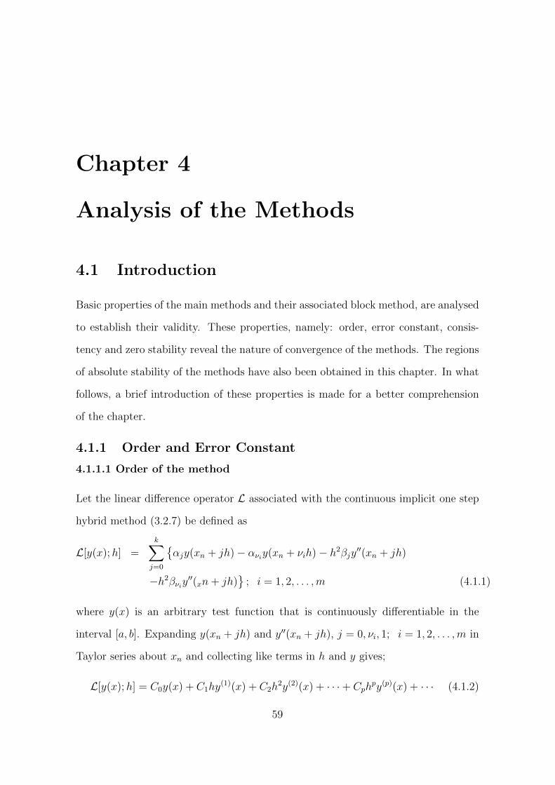
Chapter 4
Analysis of the Methods
4.1 Introduction
Basic properties of the main methods and their associated block method, are analysed
to establish their validity. These properties, namely: order, error constant, consis-
tency and zero stability reveal the nature of convergence of the methods. The regions
of absolute stability of the methods have also been obtained in this chapter. In what
follows, a brief introduction of these properties is made for a better comprehension
of the chapter.
4.1.1 Order and Error Constant
4.1.1.1 Order of the method
Let the linear difference operator L associated with the continuous implicit one step
hybrid method (3.2.7) be defined as
L[y(x);h] =k∑j=0
αjy(xn + jh)− ανiy(xn + νih)− h2βjy′′(xn + jh)
−h2βνiy′′(xn+ jh)
; i = 1, 2, . . . ,m (4.1.1)
where y(x) is an arbitrary test function that is continuously differentiable in the
interval [a, b]. Expanding y(xn + jh) and y′′(xn + jh), j = 0, νi, 1; i = 1, 2, . . . ,m in
Taylor series about xn and collecting like terms in h and y gives;
L[y(x);h] = C0y(x) + C1hy(1)(x) + C2h
2y(2)(x) + · · ·+ Cphpy(p)(x) + · · · (4.1.2)
59

Definition 4.1.1
The difference operator L and the associated continuous implicit hybrid one step
method (3.2.7) are said to be of order p if in (4.1.2) C0 = C1 = C2 = · · · = Cp =
Cp+1 = 0,Cp+2 6= 0.
Definition 4.1.2
The term Cp+2 is called the error constant and it implies that the local truncation
error is given by
tn+k = Cp+2hp+2y(p+2)(xn) +O(hp+3)
4.1.1.2 Order of the Block
The order of the block will be defined following the method of Chollom et .al . (2007)
however, with some modification to accommodate general higher order ordinary dif-
ferential equations and offstep points.
Let the implicit block hybrid one step method be defined by
∑j
α(µ)ij (t)yn+j = h2
∑j
β(µ)ij (t)fn+j, i, j = 0, ν1, . . . , νm, k (4.1.3)
where µ is the degree of the derivative of the continuous coefficients αij(t) and βij(t)
and m is the number of offstep points used.
60

In matrix form,(4.1.3) is equivalent to
α00 α01 · · · α0νm α0k
αν10 αν11 · · · αν1νm αν1k...
......
...ανm0 ανm1 · · · ανmνm ανmk
αk0 αk1 · · · αkνm αkk
α′00 α′01 · · · α′0νm α′0k
α′ν10 α′ν11 · · · α′ν1νm α′ν1k...
......
...α′νm0 α′νm1 · · · α′νmνm α′νmk
α′k0 α′k1 · · · α′kνm α′kk
yn
yn+ν1...
yn+νm
yn+1
y′n
y′n+ν1...
y′n+νm
y′n+k
=
β00 β01 · · · β0νm β0k
βν10 βν11 · · · βν1νm βν1k...
......
...βνm0 βνm1 · · · βνmνm βνmk
βk0 βk1 · · · βkνm βkk
β′00 β′01 · · · β′0νm β′0k
β′ν10 β′ν11 · · · β′ν1νm β′ν1k...
......
...β′νm0 β′νm1 · · · β′νmνm β′νmk
β′k0 β′k1 · · · β′kνm β′kk
fn
fn+ν1...
fn+νm
fn+k
.
Let
α0 = [α00, αν10, . . . , ανm0, αk0, α′00, α
′ν10, . . . , α′νm0, α
′k0]
T
αν1 = [α01, αν11, . . . , ανm1, αk1, α′01, α
′ν11, . . . , α′νm1, α
′k1]
T
...
ανm = [α01, αν11, . . . , ανm1, αk1, α′01, α
′ν11, . . . , α′νm1, α
′k1]
T
αk = [α0k, α1k, . . . , ανmk, αkk, α′0k, α
′ν1k, . . . , α′νmk, α
′kk]
T .
Similarly,
β0 = [β00, βν10, . . . , βνm0, βk0, β′00, β
′ν10, . . . , β′νm0, β
′k0]
T
β1 = [β01, βν11, . . . , βνm1, βk1, β′01, β
′ν11, . . . , β′νm1, β
′k1]
T
...
βνm = [β01, βν11, . . . , βνm1, βk1, β′01, β
′ν11, . . . , β′νm1, β
′k1]
T
βk = [β0k, β1k, . . . , βνmk, βkk, β′0k, β
′ν1k, . . . , β′νmk, β
′kk]
T .
Then, the linear difference operator, L, associated with the implicit block hybrid one
61

step method (4.1.3) is described by the formula
L[y(x);h] =∑j
[αjy(xn + jh)− h2βjy′′(xn + jh)
], j = 0, ν1, . . . , νm, k, (4.1.4)
where y(x) is an arbitrary test function continuously differentiable on [a, b]. Expand-
ing y(xn + jh) and y′′(xn + jh), j = 0, ν1, . . . , νm, k in Taylor series and collecting
terms in (4.1.4) gives
L[y(x);h] = c0y(x) + c1hy(1)(x) + c2h
2y(2)(x) + · · ·+ cphpy(p)(x) (4.1.5)
where the ci, i = 0, 1, . . . , p are vectors.
Definition 4.1.3
The one-step implicit hybrid block linear method (4.1.3) and the associated linear
difference operator (4.1.4) are said to have order q if c0 = c1 = · · · = cp = cp+1 = 0
and cp+2 6= 0.
Definition 4.1.4
The term cp+2 is called the error constant and implies that the local truncation error
for the implicit block hybrid formula is given by
tn+k = cp+2hp+2y(p+2)(xn) +O(hp+3) (4.1.6)
4.1.2 Consistency
Definition 4.1.5
Given a continuous implicit one step hybrid method (3.2.7), the first and second
characteristic polynomials are defined as
ρ(z) =k∑j=0
αjzj (4.1.7)
σ(z) =k∑j=0
βjzj (4.1.8)
62

where z is the principal root, αk 6= 0 and α20 + β2
0 6= 0.
Definition 4.1.6
The continuous implicit one step hybrid method (3.2.7) is said to be consistent if it
satisfies the following conditions:
(i) the order p ≥ 1
(ii)k∑j=0
αj = 0
(iii) ρ(1) = ρ′(1) = 0 and
(iv) ρ′′(1) = 2!σ(1)
Remark
Condition (i) is a sufficient condition for the associated block method to be consistent
i.e., p ≥ 1 (Jator, 2007).
4.1.3 Zero Stability
Definition 4.1.7
The continuous implicit one step hybrid method (3.2.7) is said to be zero-stable if no
root of the first characteristic polynomial ρ(z) has modulus greater than one, and if
every root of modulus one has multiplicity not greater than one.
Definition 4.1.8
The implicit hybrid block method (3.2.12) is said to be zero stable if the roots zs, s =
1, . . . , n of the first characteristic polynomial ρ(z), defined by
ρ(z) = det[zA− E] (4.1.9)
satisfies |zs| ≤ 1 and every root with |zs| = 1 has multiplicity not exceeding two in
the limit as h→ 0.
63

4.1.4 Convergence
The convergence of the continuous implicit hybrid one step method (3.2.7) is con-
sidered in the light of the basic properties discussed earlier in conjunction with the
fundamental theorem of Dahlquist (Henrici,1962) for linear multistep methods. In
what follows, we state Dahlquist’s theorem without proof.
Theorem 4.1.1
The necessary and sufficient condition for a linear multistep method to be convergent
is for it to be consistent and zero stable.
Remark
The numerical methods derived here are considered to be convergent in the limit as
h→ 0 by Theorem 4.1.1.
4.1.5 Region of Absolute Stability
4.1.5.1 Region of absolute stability of the main methods
Consider the stability polynomial
Π(z, h) = ρ(z)− hσ(z) = 0 (4.1.10)
where h = h2λ2 and λ =df
dyare assumed constant.
The polynomial equation (4.1.10) is obtained by applying the continuous implicit
hybrid one step method (3.2.7) to the scalar test problem;
y′′ = −λ2y (4.1.11)
Definition 4.1.9
The method (3.2.7) is said to be absolutely stable if for a given h all the roots zs of
(4.1.10) satisfy |zs| < 1, s = 1, 2, . . . , n, where h = λh.
64
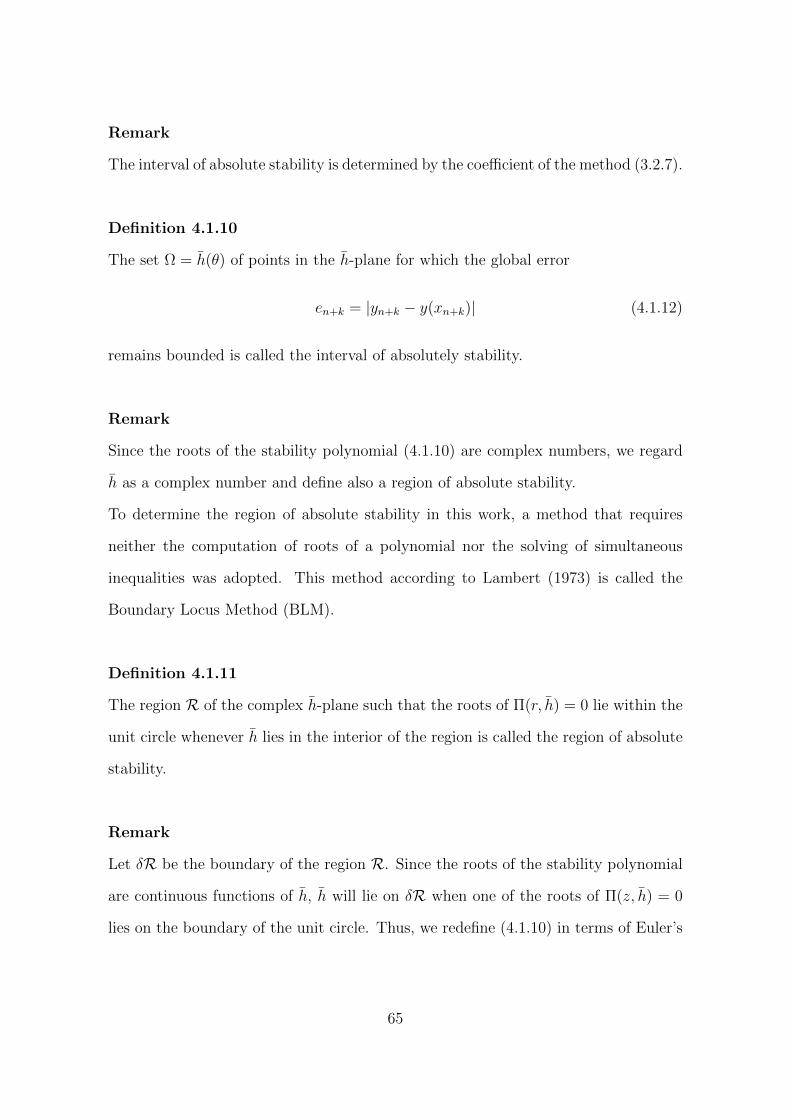
Remark
The interval of absolute stability is determined by the coefficient of the method (3.2.7).
Definition 4.1.10
The set Ω = h(θ) of points in the h-plane for which the global error
en+k = |yn+k − y(xn+k)| (4.1.12)
remains bounded is called the interval of absolutely stability.
Remark
Since the roots of the stability polynomial (4.1.10) are complex numbers, we regard
h as a complex number and define also a region of absolute stability.
To determine the region of absolute stability in this work, a method that requires
neither the computation of roots of a polynomial nor the solving of simultaneous
inequalities was adopted. This method according to Lambert (1973) is called the
Boundary Locus Method (BLM).
Definition 4.1.11
The region R of the complex h-plane such that the roots of Π(r, h) = 0 lie within the
unit circle whenever h lies in the interior of the region is called the region of absolute
stability.
Remark
Let δR be the boundary of the region R. Since the roots of the stability polynomial
are continuous functions of h, h will lie on δR when one of the roots of Π(z, h) = 0
lies on the boundary of the unit circle. Thus, we redefine (4.1.10) in terms of Euler’s
65
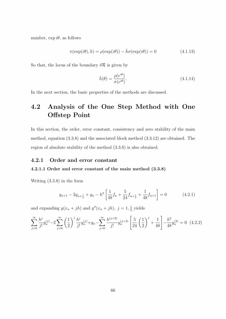
number, exp iθ, as follows
π(exp(iθ), h) = ρ(exp(iθ))− hσ(exp(iθ)) = 0 (4.1.13)
So that, the locus of the boundary δR is given by
h(θ) =ρ(eiθ)
σ(eiθ). (4.1.14)
In the next section, the basic properties of the methods are discussed.
4.2 Analysis of the One Step Method with One
Offstep Point
In this section, the order, error constant, consistency and zero stability of the main
method, equation (3.3.8) and the associated block method (3.3.12) are obtained. The
region of absolute stability of the method (3.3.8) is also obtained.
4.2.1 Order and error constant
4.2.1.1 Order and error constant of the main method (3.3.8)
Writing (3.3.8) in the form
yn+1 − 2yn+ 12
+ yn − h2[
1
48fn +
5
24fn+ 1
2+
1
48fn+1
]= 0 (4.2.1)
and expanding y(xn + jh) and y′′(xn + jh), j = 1, 12
yields
∞∑j=0
hj
j!y(j)n −2
∞∑j=0
(1
2
)jhj
j!y(j)n +yn−
∞∑j=0
h(j+2)
j!y(j+2)n
[5
24
(1
2
)j+
1
48
]−h
2
48y(2)n = 0 (4.2.2)
66

Collecting terms in powers of h and y gives the following constants
c0 = 1− 2 + 1 = 0
c1 = 1− 1 = 0
c2 =1
2− 1
4− 10
48− 1
48− 1
48= 0
c3 =1
6− 1
24− 1
48− 5
48= 0
c4 =1
24− 1
192− 1
96− 5
192= 0
c5 =1
120− 1
1920− 1
288− 5
1152= 0
c6 =1
720− 23040
−1
1152− 1
221184=
401609
849231360= −4.7291× 10⁻⁴
Hence, the main method is of order p = 4 with error constant cp+2 = −4.7291×10⁻⁴.
4.2.1.2 Order of the block method (3.3.12)
Let (3.3.12) be expressed in the form
1 0 0 0
0 1 0 0
0 0 1 0
0 0 0 1
yn+ 12
yn+1
y′n+ 1
2
y′n+1
−
1 h2
1 h
0 1
0 1
yn
y′n
−
7h2
96
h2
6
5h24
h6
[fn]−
h2
16−h2
96
h2
30
h3− h
24
2h3
h6
fn+ 1
2
fn+1
= 0 (4.2.3)
Expand (4.2.3) in Taylor series about xn in the form
∑∞j=0
( 12)jhj
j!y(j)n − yn − h
2y(1)n − 7h2
96y(2)n −
∑∞j=0
hj+2
j!y(j+2)n
[116
(12
)j − 196
]∑∞
j=0hj
j!y(j)n − yn − hy(1)n − h2
6y(2)n −
∑∞j=0
hj+2
j!y(j+2)n
[13
(12
)j − 0]
∑∞j=0
( 12h)
j
j!y(j+1)n − y(1)n − 5h
24y(2)n −
∑∞j=0
hj+1
j!y(j+2)n
[13
(12
)j − 124
]∑∞
j=0hj
j!y(j+1)n − y(1)n − h
6y(2)n −
∑∞j=0
hj+1
j!y(j+2)n
[23
(12
)j − 16
]
=
0
0
0
0
(4.2.4)
67
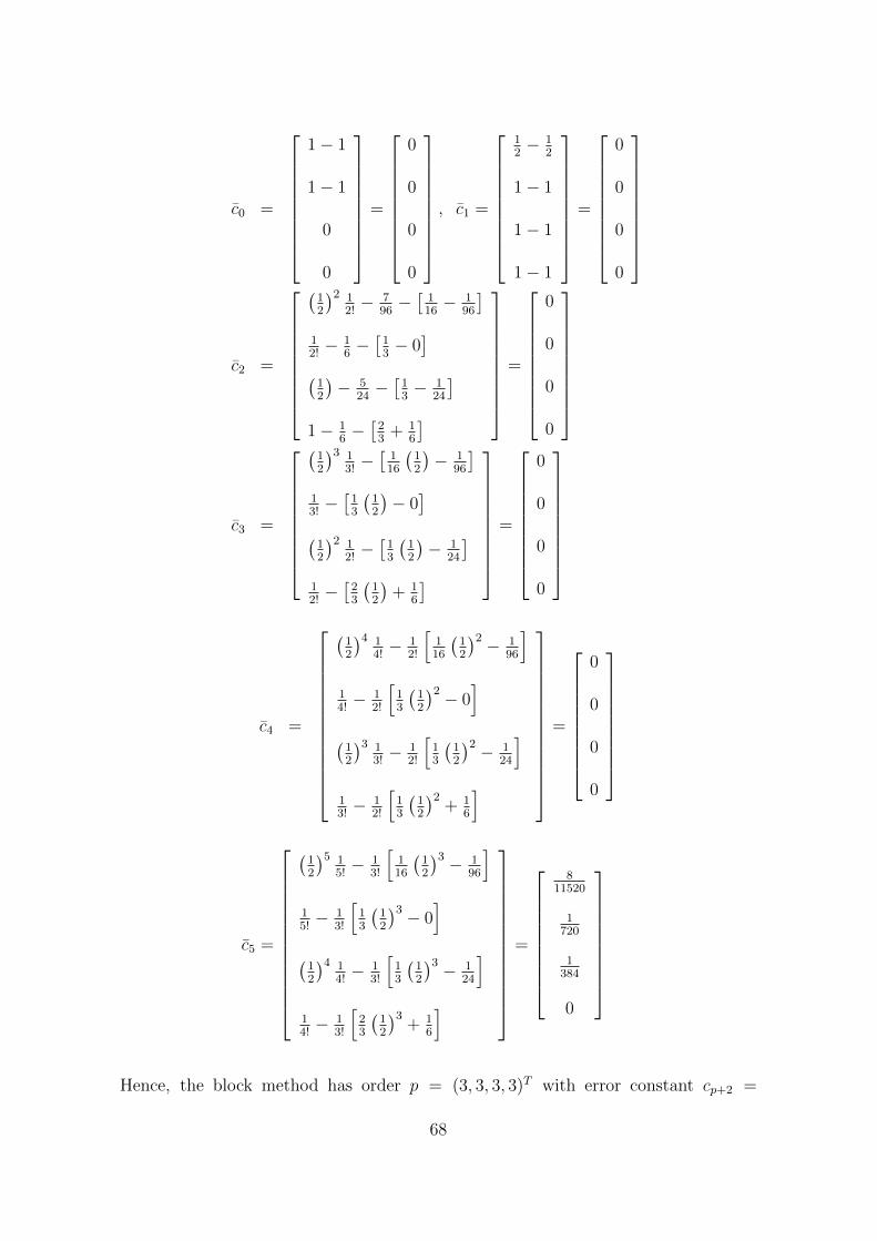
c0 =
1− 1
1− 1
0
0
=
0
0
0
0
, c1 =
12− 1
2
1− 1
1− 1
1− 1
=
0
0
0
0
c2 =
(12
)2 12!− 7
96−[
116− 1
96
]12!− 1
6−[13− 0]
(12
)− 5
24−[13− 1
24
]1− 1
6−[23
+ 16
]
=
0
0
0
0
c3 =
(12
)3 13!−[
116
(12
)− 1
96
]13!−[13
(12
)− 0]
(12
)2 12!−[13
(12
)− 1
24
]12!−[23
(12
)+ 1
6
]
=
0
0
0
0
c4 =
(12
)4 14!− 1
2!
[116
(12
)2 − 196
]14!− 1
2!
[13
(12
)2 − 0]
(12
)3 13!− 1
2!
[13
(12
)2 − 124
]13!− 1
2!
[13
(12
)2+ 1
6
]
=
0
0
0
0
c5 =
(12
)5 15!− 1
3!
[116
(12
)3 − 196
]15!− 1
3!
[13
(12
)3 − 0]
(12
)4 14!− 1
3!
[13
(12
)3 − 124
]14!− 1
3!
[23
(12
)3+ 1
6
]
=
811520
1720
1384
0
Hence, the block method has order p = (3, 3, 3, 3)T with error constant cp+2 =
68

( 811520
, 1720, 1384, 0)T .
4.2.2 Consistency
4.2.2.1 Consistency of the main method (3.3.8)
The first and second characteristic polynomials of method (3.3.8) are given by
ρ(z) = z − 2z1/2 + 1
and
σ(z) =z + 10r1/2 + 1
48
By definition (4.1.6), the method (3.3.8) is consistent since it satisfies the following:
(i) the order of the method is p = 4 ≥ 1.
(ii) α0 = 1, α 12
= −2 and α1 = 1. Thus,∑j
αj = 1− 2 + 1 = 0, j = 0,1
2, 1
(iii) ρ(1) = 1− 2− 1 = 0
ρ′(z) = 1− r−12
For r = 1
ρ′(1) = 1− 1 = 0
... ρ(1) = ρ′(1) = 0
(iv) ρ′′(z) = 12z−3/2
ρ′′(1) = 12
σ(1) = 1+10+148 = 1
4
2!σ(1) = 2(14
)= 1
2
... ρ′′(1) = 2!σ(1)
Similarly, the block method (3.3.12) is consistent by condition (i) of definition (4.1.6).
69
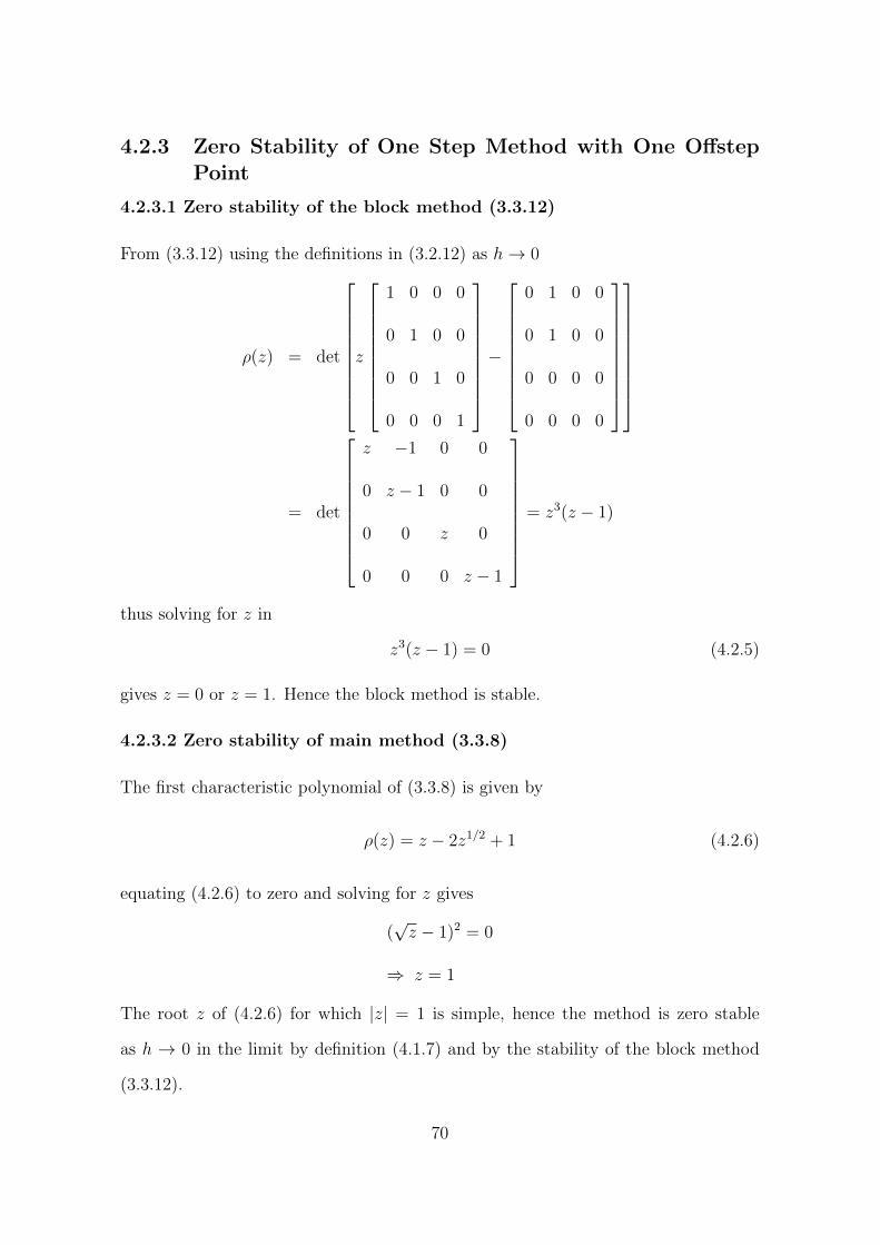
4.2.3 Zero Stability of One Step Method with One OffstepPoint
4.2.3.1 Zero stability of the block method (3.3.12)
From (3.3.12) using the definitions in (3.2.12) as h→ 0
ρ(z) = det
z
1 0 0 0
0 1 0 0
0 0 1 0
0 0 0 1
−
0 1 0 0
0 1 0 0
0 0 0 0
0 0 0 0
= det
z −1 0 0
0 z − 1 0 0
0 0 z 0
0 0 0 z − 1
= z3(z − 1)
thus solving for z in
z3(z − 1) = 0 (4.2.5)
gives z = 0 or z = 1. Hence the block method is stable.
4.2.3.2 Zero stability of main method (3.3.8)
The first characteristic polynomial of (3.3.8) is given by
ρ(z) = z − 2z1/2 + 1 (4.2.6)
equating (4.2.6) to zero and solving for z gives
(√z − 1)2 = 0
⇒ z = 1
The root z of (4.2.6) for which |z| = 1 is simple, hence the method is zero stable
as h → 0 in the limit by definition (4.1.7) and by the stability of the block method
(3.3.12).
70

4.2.4 Convergence
Following Theorem 4.1.1, the method (3.3.8) is convergent since it satisfies the nec-
essary and sufficient conditions of consistency and zero stability.
4.2.5 Region of Absolute Stability of the one step Methodwith One Offstep Point
From (3.3.8), the first and second characteristic polynomial are as follows
ρ(z) = z − 2z1/2 + 1. (4.2.7)
σ(z) =1
48z +
10
48z1/2 +
1
48(4.2.8)
so that the boundary of the region of absolute stability is
h(z) =ρ(z)
σ(z)=
48(z − 2z1/2 + 1)
z + 10z1/2 + 1(4.2.9)
Let z = eiθ, therefore (4.2.9) becomes
h(θ) =48(eiθ − 2ei
12θ + 1)
eiθ + 10ei12θ + 1
(4.2.10)
for eiθ = cos θ + i sin θ, (4.2.10)reduces after some manipulation to
h(θ) =768 cos 1
2θ + 96 cos θ − 864
40 cos 12θ + 2 cos θ + 102
(4.2.11)
Evaluating (4.2.11) at intervals of 300 gives the following results;
Table 1. The boundaries of the region of absolute stability of the one step 1 offstep point
method.
θ 0 300 600 900 1200 1500 1800
h(θ) 0 -0.27 -1.10 -2.46 -4.36 -6.77 -9.60
Thus, the interval of absolute stability from table 1 is (-9.6,0). The region of
absolute stability is shown in figure 4.1
Remark
The locus is symmetric about the x-axis that is, x(−θ) = x(θ).
71

Figure 4.1: Region of Absolute stability of the One-Step Method with One offsteppoint
4.3 Analysis of the One Step Method with Two
Offstep Points
In this section, the order, error constant, consistency and zero stability of the method
(3.3.21a) and its associated block method (3.3.25) are obtained. The region of abso-
lute stability of the method (3.3.21a) is also obtained.
4.3.1 Order and Error Constant
4.3.1.1 Order and error constant of the main method (3.3.21a)
Let (3.3.21a) be written in the form
yn+1 − 2yn+ 23
+ yn+ 13− h2
[1
108fn+ 1
3+
5
54fn+ 2
3+
1
108fn+1
]= 0 (4.3.1)
Expanding (4.3.1) in Taylor series in the form
∞∑j=0
hj
j!y(j)n − 2
∞∑j=0
(23
)jhj
j!y(j)n +
∞∑j=0
(13
)jhj
j!y(j)n −
∞∑j=0
h(j+2)
j!y(j+2)n
[1
108
(1
3
)j
+5
54
(2
3
)j+
1
108
](4.3.2)
72
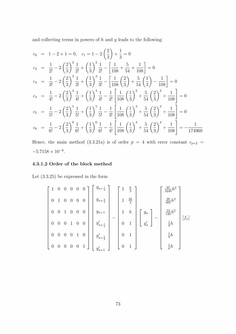
and collecting terms in powers of h and y leads to the following:
c0 = 1− 2 + 1 = 0, c1 = 1− 2
(2
3
)+
1
3= 0
c2 =1
2!− 2
(2
3
)21
2!+
(1
3
)21
2!−[
1
108+
5
54+
1
108
]= 0
c3 =1
3!− 2
(2
3
)31
3!+
(1
3
)31
3!−[
1
108
(2
3
)+
5
54
(1
3
)− 1
108
]= 0
c4 =1
4!− 2
(2
3
)41
4!+
(1
3
)41
4!− 1
2!
[1
108
(1
3
)2
+5
54
(2
3
)2
+1
108
]= 0
c5 =1
5!− 2
(2
3
)51
5!+
(1
3
)51
5!− 1
3!
[1
108
(1
3
)3
+5
54
(2
3
)3
+1
108
]= 0
c6 =1
6!− 2
(2
3
)61
6!+
(1
3
)61
6!− 1
4!
[1
108
(1
3
)4
+5
54
(2
3
)4
+1
108
]= − 1
174960
Hence, the main method (3.3.21a) is of order p = 4 with error constant cp+2 =
−5.7158× 10⁻⁶.
4.3.1.2 Order of the block method
Let (3.3.25) be expressed in the form
1 0 0 0 0 0
0 1 0 0 0 0
0 0 1 0 0 0
0 0 0 1 0 0
0 0 0 0 1 0
0 0 0 0 0 1
yn+ 13
yn+ 23
yn+1
y′n+ 1
3
y′n+ 2
3
y′n+1
−
1 h3
1 2h3
1 h
0 1
0 1
0 1
yn
y′n
−
973240
h2
28405h2
13120h2
18h
19h
18h
[fn]
73
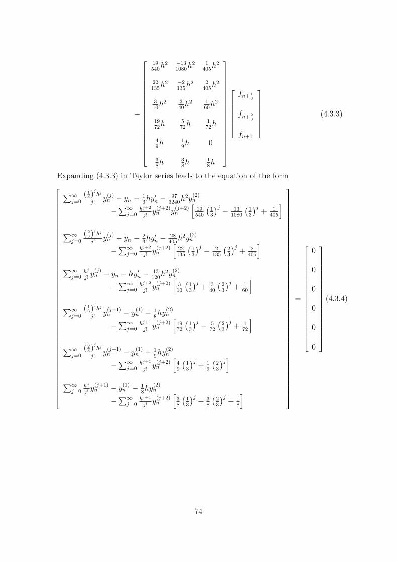
−
19540h2 −13
1080h2 1
405h2
22135h2 −2
135h2 2
405h2
310h2 3
40h2 1
60h2
1972h 5
72h 1
72h
49h 1
9h 0
38h 3
8h 1
8h
fn+ 1
3
fn+ 23
fn+1
(4.3.3)
Expanding (4.3.3) in Taylor series leads to the equation of the form
∑∞j=0
( 13)
jhj
j!y(j)n − yn − 1
3hy′n − 97
3240h2y
(2)n
−∑∞
j=0hj+2
j!y(j+2)n y
(j+2)n
[19540
(13
)j − 131080
(13
)j+ 1
405
]∑∞
j=0
( 23)
jhj
j!y(j)n − yn − 2
3hy′n − 28
405h2y
(2)n
−∑∞
j=0hj+2
j!y(j+2)n
[22135
(13
)j − 2135
(23
)j+ 2
405
]∑∞
j=0hj
j!y(j)n − yn − hy′n − 13
120h2y
(2)n
−∑∞
j=0hj+2
j!y(j+2)n
[310
(13
)j+ 3
40
(23
)j+ 1
60
]∑∞
j=0
( 13)
jhj
j!y(j+1)n − y(1)n − 1
8hy
(2)n
−∑∞
j=0hj+1
j!y(j+2)n
[1972
(13
)j − 572
(23
)j+ 1
72
]∑∞
j=0
( 23)
jhj
j!y(j+1)n − y(1)n − 1
9hy
(2)n
−∑∞
j=0hj+1
j!y(j+2)n
[49
(13
)j+ 1
9
(23
)j]∑∞
j=0hj
j!y(j+1)n − y(1)n − 1
8hy
(2)n
−∑∞
j=0hj+1
j!y(j+2)n
[38
(13
)j+ 3
8
(23
)j+ 1
8
]
=
0
0
0
0
0
0
(4.3.4)
74

and collecting terms in powers of h and y leads to the following:
c0 =
1− 1
1− 1
1− 10
0
0
=
0
0
0
0
0
0
, c1 =
13− 1
3
23− 2
3
1− 1
1− 1
1− 1
1− 1
=
0
0
0
0
0
0
c2 =
(13
)2 12!− 97
3240−[
19540− 13
10801
405
](23
)2 12!− 28
405−[
22135− 2
135+ 2
405
]12!− 13
120−[
310
+ 340
+ 160
]13− 1
8−[1972− 5
72+ 1
72
]23− 1
9−[49
+ 19
]1− 1
8−[38
+ 38
+ 18
]
=
0
0
0
0
0
0
c3 =
(13
)3 13!−[
19540
(13
)− 13
1080
(23
)+ 1
405
](23
)3 13!−[
22135
(13
)− 2
135
(23
)+ 2
405
]13!−[
310
(13
)+ 3
40
(23
)+ 1
60
](13
)2 12!−[1972
(13
)− 5
72
(23
)+ 1
72
](23
)2 12!−[49
(13
)+ 1
9
(23
)]12!−[38
(13
)+ 3
8
(23
)+ 1
8
]
=
0
0
0
0
0
0
75

c4 =
(13
)4 14!− 1
2!
[19540
(13
)2 − 131080
(23
)2+ 1
405
](23
)3 14!− 1
2!
[22135
(13
)2 − 2135
(23
)2+ 2
405
]14!− 1
2!
[310
(13
)2+ 3
40
(23
)2+ 1
60
](13
)3 13!− 1
2!
[1972
(13
)2 − 572
(23
)2+ 1
72
](23
)3 13!− 1
2!
[49
(13
)2+ 1
9
(23
)2]13!− 1
2!
[38
(13
)2+ 3
8
(23
)2+ 1
8
]
=
0
0
0
0
0
0
c5 =
(13
)5 15!− 1
3!
[19540
(13
)3 − 131080
(23
)3+ 1
405
](23
)5 15!− 1
3!
[22135
(13
)2 − 2135
(23
)3+ 2
405
]15!− 1
3!
[310
(13
)3+ 3
40
(23
)3+ 1
60
](13
)4 14!− 1
3!
[1972
(13
)3 − 572
(23
)3+ 1
72
](23
)4 14!− 1
3!
[49
(13
)3 − 19
(23
)3]14!− 1
3!
[38
(13
)3+ 3
8
(23
)3+ 1
8
]
=
0
0
0
0
0
0
c6 =
(13
)6 16!− 1
4!
[19540
(13
)4 − 131080
(23
)4+ 1
405
](23
)6 16!− 1
4!
[22135
(13
)4 − 2135
(23
)4+ 2
405
]16!− 1
4!
[310
(13
)4+ 3
40
(23
)4+ 1
60
](13
)5 15!− 1
4!
[1972
(13
)4 − 572
(23
)4 + 1
72
](23
)5 15!− 1
4!
[49
(13
)4+ 1
9
(23
)4]15!− 1
4!
[38
(13
)4+ 3
8
(23
)4+ 1
8
]
=
− 7349920
− 121870
− 112960
− 19174960
− 121870
− 16480
Thus the block method (3.3.25) has order p = (4, 4, 4, 4)T with the error constant
cp+2 =( −7349920
, − 121870
, − 121960
, − 19174960
, − 121870
, − 16480
)T.
76

4.3.2 Consistency of the Method
The block method (3.3.25) has order p = (4, 4, 4, 4)T ≥ 1, therefore it is consistent by
condition (i) of definition (4.1.6).
Following the consistency of the block method (3.3.25), the consistency of the
main method (3.3.21a) is shown by conditions (i) - (iv) of definition (4.1.6) below.
However, consider the first and second characteristic polynomials of method (3.3.21a)
given by
ρ(z) = z − 2z2/3 + z1/3 (4.3.5)
and
σ(z) =z + 10z2/3 + z1/3
108(4.3.6)
Now by definition (4.1.6),
Condition (i)
The main method (3.3.21a) has been shown to have order
p = 4 ≥ 1
Condition (ii)
α1/3 = 1, α2/3 = −2 and α1 = 1∑αj = 1 − 2 + 1 = 1, j =
1
3,2
3, 1
Condition (iii)
ρ′(z) =1
3z−2/3
(3z2/3 − 4z1/3 + 1
)ρ′(1) =
1
3(3− 4 + 1) = 0
ρ(1) = 1− 2 + 1 = 0
⇒ ρ(1) = ρ′(1) = 0
77

Condition (iv)
ρ′′(z) =2
9z−5/3
(2z1/3 − 1
)⇒ ρ′′(1) =
2
9(2− 1) =
2
9
σ(1) =1 + 10 + 1
108=
12
108=
3
27=
1
9
2!σ(1) = 2
(1
9
)=
2
9
⇒ ρ′′(1) = 2!σ(1)
Therefore the method (3.3.21a) is consistent.
4.3.3 Zero Stability of the Method
4.3.3.1 Zero stability of the Block Method (3.3.25)
From (3.3.25) using definitions in (3.2.12) as h→ 0 we have
ρ(z) = det
z
1 0 0 0 0 0
0 1 0 0 0 0
0 0 1 0 0 0
0 0 0 1 0 0
0 0 0 0 1 0
0 0 0 0 0 1
−
0 0 1 0 0 0
0 0 1 0 0 0
0 0 1 0 0 0
0 0 0 0 0 0
0 0 0 0 0 0
0 0 0 0 0 0
= det
z 0 −1 0 0 0
0 z −1 0 0 0
0 0 z − 1 0 0 0
0 0 0 z 0 0
0 0 0 0 z 0
0 0 0 r 0 z
= z5(z − 1)
78
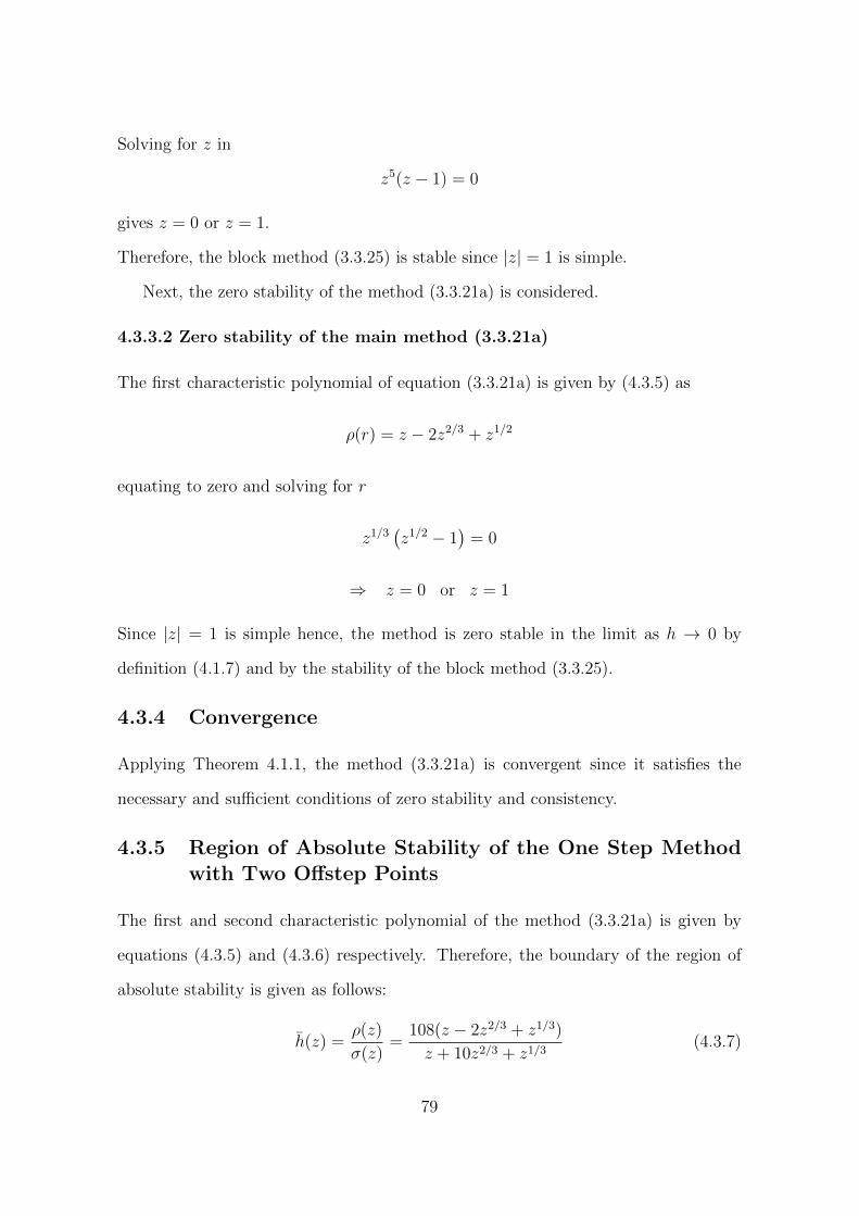
Solving for z in
z5(z − 1) = 0
gives z = 0 or z = 1.
Therefore, the block method (3.3.25) is stable since |z| = 1 is simple.
Next, the zero stability of the method (3.3.21a) is considered.
4.3.3.2 Zero stability of the main method (3.3.21a)
The first characteristic polynomial of equation (3.3.21a) is given by (4.3.5) as
ρ(r) = z − 2z2/3 + z1/2
equating to zero and solving for r
z1/3(z1/2 − 1
)= 0
⇒ z = 0 or z = 1
Since |z| = 1 is simple hence, the method is zero stable in the limit as h → 0 by
definition (4.1.7) and by the stability of the block method (3.3.25).
4.3.4 Convergence
Applying Theorem 4.1.1, the method (3.3.21a) is convergent since it satisfies the
necessary and sufficient conditions of zero stability and consistency.
4.3.5 Region of Absolute Stability of the One Step Methodwith Two Offstep Points
The first and second characteristic polynomial of the method (3.3.21a) is given by
equations (4.3.5) and (4.3.6) respectively. Therefore, the boundary of the region of
absolute stability is given as follows:
h(z) =ρ(z)
σ(z)=
108(z − 2z2/3 + z1/3)
z + 10z2/3 + z1/3(4.3.7)
79

Let z = eiθ, therefore, (4.3.7) becomes
h(θ) =108(eiθ − 2ei
23θ + ei
13θ)
eiθ + 10ei23θ + ei
13θ
(4.3.8)
Since eiθ = cos θ + i sin θ, (4.3.8) reduces after some manipulations to
h(θ) =1728 cos 1
3θ + 216 cos 2
3θ − 1944
40 cos 13θ + 2 cos 2
3θ + 102
(4.3.9)
Evaluating (4.3.9) at intervals of 300 gives the following results;
Table 2. The boundaries of the region of absolute stability of the one step 2 offstep points
method.
θ 0 300 600 900 1200 1500 1800
h(θ) 0 −0.27 −1.10 −2.47 −4.38 −6.84 −9.82
From table 2, the interval of absolute stability is (−9.82, 0). The region of absolute
stability is shown in figure 4.2.
Remark The locus is symmetric about the x-axis as x(−θ) = x(θ)
Figure 4.2: Region of Absolute Stability of the Continuous One-Step Method withTwo Offstep Points
80
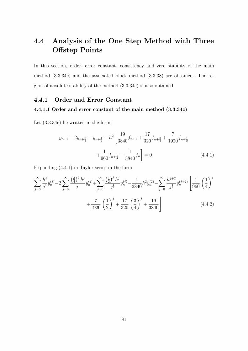
4.4 Analysis of the One Step Method with Three
Offstep Points
In this section, order, error constant, consistency and zero stability of the main
method (3.3.34c) and the associated block method (3.3.38) are obtained. The re-
gion of absolute stability of the method (3.3.34c) is also obtained.
4.4.1 Order and Error Constant
4.4.1.1 Order and error constant of the main method (3.3.34c)
Let (3.3.34c) be written in the form:
yn+1 − 2yn+ 34
+ yn+ 12− h2
[19
3840fn+1 +
17
320fn+ 3
4+
7
1920fn+ 1
2
+1
960fn+ 1
4− 1
3840fn
]= 0 (4.4.1)
Expanding (4.4.1) in Taylor series in the form
∞∑j=0
hj
j!y(j)n −2
∞∑j=0
(34
)jhj
j!y(j)n +
∞∑j=0
(12
)jhj
j!y(j)n −
1
3840h2y(2)n −
∞∑j=0
hj+2
j!y(j+2)n
[1
960
(1
4
)j
+7
1920
(1
2
)j+
17
320
(3
4
)j+
19
3840
](4.4.2)
81

and collecting terms in powers of h and y leads to the following:
c0 = 1− 2− 1 = 0
c1 = 1− 2
(3
4
)+
1
2= 0
c2 =1
2!− 2
(3
4
)21
2!+
(1
2
)21
2!− 1
3840−[
1
960+
7
1920+
17
320+
19
3840
]= 0
c3 =1
3!− 2
(3
4
)31
3!+
(1
2
)31
3!−[
1
960
(1
4
)+
7
1920
(1
2
)+
17
320
(3
4
)+
19
3840
]= 0
c4 =1
4!− 2
(3
4
)41
4!+
(1
2
)41
4!− 1
2!
[1
960
(1
4
)2
+7
1920
(1
2
)2
+17
320
(3
4
)2
+19
3840
]= 0
c5 =1
5!− 2
(3
4
)51
5!+
(1
2
)51
5!− 1
3!
[1
960
(1
4
)3
+7
1920
(1
2
)3
+17
320
(3
4
)3
+19
3840
]= 0
c6 =1
6!− 2
(3
4
)61
6!+
(1
2
)61
6!− 1
4!
[1
960
(1
4
)4
+7
1920
(1
2
)4
+17
320
(3
4
)4
+19
3840
]= 0
c7 =1
7!− 2
(3
4
)71
7!+
(1
2
)71
7!− 1
5!
[1
960
(1
4
)5
+7
1920
(1
2
)5
+17
320
(3
4
)5
+19
3840
]=
1
3932160
Hence, the method (3.3.34c) is of order p = 5 with error constant cp+2 = 2.5431×10⁻⁷.
82
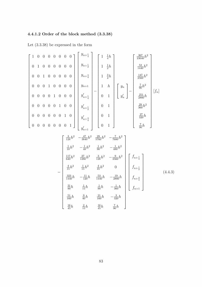
4.4.1.2 Order of the block method (3.3.38)
Let (3.3.38) be expressed in the form
1 0 0 0 0 0 0 0
0 1 0 0 0 0 0 0
0 0 1 0 0 0 0 0
0 0 0 1 0 0 0 0
0 0 0 0 1 0 0 0
0 0 0 0 0 1 0 0
0 0 0 0 0 0 1 0
0 0 0 0 0 0 0 1
yn+ 14
yn+ 12
yn+ 34
yn+1
y′n+ 1
4
y′n+ 1
2
y′n+ 3
4
y′n+1
−
1 14h
1 12h
1 34h
1 h
0 1
0 1
0 1
0 1
yn
y′n
−
36723040
h2
531440
h2
1472560
h2
790h2
2512880
h
29360h2
27320h
790h
[fn]
−
3128h2 − 47
3840h2 29
5760h2 − 7
7680h2
110h2 − 1
48h2 1
90h2 − 1
480h2
117640h2 27
1280h2 3
128h2 − 9
2560h2
415h2 1
15h2 4
45h2 0
3231440
h − 11120h 53
1440h − 19
2880h
3190h 1
15h 1
90h − 1
360h
51160h 9
40h 21
160h − 3
320h
1645h 2
15h 16
45h 7
90h
fn+ 14
fn+ 12
fn+ 34
fn+1
(4.4.3)
83

Expanding (4.4.3) in Taylor series in the form
∞∑j=0
(14
)jhj
j!y(j)n − yn −
1
4hy(1)n −
367
23040h2y(2)n
−∑∞
j=0hj+2
j!y(j+2)n
[3
128
(14
)j − 473840
(12
)j+ 29
5760
(34
)j − 77680
]∞∑j=0
(12
)jhj
j!y(j)n − yn −
1
2hy(1)n −
53
1440h2y(2)n
−∑∞
j=0hj+2
j!y(j+2)n
[110
(14
)j − 148
(12
)j+ 1
90
(34
)j − 1480
]∞∑j=0
(34
)jhj
j!y(j)n − yn −
3
4hy(1)n −
147
2560h2y(2)n
−∑∞
j=0hj+2
j!y(j+2)n
[117640
(14
)j+ 27
1280
(12
)j+ 3
128
(34
)j − 92560
]∞∑j=0
hj
j!y(j)n − yn − hy(1)n −
7
90h2y(2)n
−∑∞
j=0hj+2
j!y(j+2)n
[415
(14
)j+ 1
15
(12
)j+ 4
45
(34
)j]∞∑j=0
(14
)jhj
j!y(j+1)n − y(1)n −
251
2880hy(2)n
−∑∞
j=0hj+1
j!y(j+2)n
[3231440
(14
)j − 11120
(12
)j+ 53
1440
(34
)j − 192880
]∞∑j=0
(12
)jhj
j!y(j+1)n − y(1)n −
29
360hy(2)n
−∑∞
j=0hj+1
j!y(j+2)n
[3190
(14
)j+ 1
15
(12
)j+ 1
90
(34
)j − 1360
]∞∑j=0
(34
)jhj
j!y(j+1)n − y(1)n −
27
320hy(2)n
−∑∞
j=0hj+1
j!y(j+2)n
[51160
(14
)j+ 9
40
(12
)j+ 21
160
(34
)j − 3320
]∞∑j=0
hj
j!y(j+1)n − y(1)n −
7
90hy(2)n
−∑∞
j=0hj+1
j!y(j+2)n
[1645
(14
)j+ 2
15
(12
)j+16
45
(34
)j+ 7
90
]
=
0
0
0
0
0
0
0
0
(4.4.4)
84

and collecting terms in powers of h and y leads to the following results:
c0 =
1− 1
1− 1
1− 1
1− 10
0
0
0
=
0
0
0
0
0
0
0
0
, c1 =
14− 1
4
12− 1
2
34− 3
4
1− 1
1− 1
1− 1
1− 1
1− 1
=
0
0
0
0
0
0
0
0
c2 =
(14
)2 12!− 367
23040−[
3128− 47
3840+ 29
5760− 7
7680
](12
)2 12!− 53
1440−[
110− 1
48+ 1
90− 1
480
](34
)2 12!− 147
2560−[117640
+ 271280
+ 3128− 9
2560
]12!− 7
90−[
415
+ 115
+ 445
]14− 251
2880−[
3231440− 11
120+ 53
1440− 19
2880
]12− 29
360−[3190
+ 115
+ 190− 1
360
]34− 27
320−[
51160
+ 940
+ 21160− 3
320
]1− 7
90−[1695
+ 215
+ 1645
+ 790
]
=
0
0
0
0
0
0
0
0
85

c3 =
(14
)3 13!−[
3128
(14
)− 47
3840
(14
)+ 29
5760
(34
)− 7
7680
](12
)3 13!−[
110
(14
)− 1
48
(12
)+ 1
90
(34
)− 1
480
](34
)3 13!−[117640
(14
)+ 27
1280
(12
)+ 3
128
(34
)− 9
2560
]13!−[
415
(14
)+ 1
15
(12
)+ 4
45
(34
)](14
)2 12!−[
3231440
(14
)− 11
120
(12
)+ 53
1440
(34
)− 19
2880
](12
)2 12!−[3190
(14
)+ 1
15
(12
)+ 1
90
(34
)− 1
360
](34
)2 12!−[
51160
(14
)+ 9
40
(12
)+ 21
160
(34
)− 3
320
]12!−[1645
(14
)+ 2
15
(12
)+ 16
45
(34
)+ 7
90
]
=
0
0
0
0
0
0
0
0
c4 =
(14
)4 14!− 1
2!
[3
125
(14
)2 − 473840
(12
)2+ 29
5760
(34
)2 − 77680
](12
)4 14!− 1
2!
[110
(14
)2 − 148
(12
)2+ 1
90
(34
)2 − 1480
](34
)4 14!− 1
2!
[117640
(14
)2+ 27
1280
(12
)2+ 3
128
(34
)2 − 92560
]14!− 1
2!
[415
(14
)2+ 1
15
(12
)2+ 4
45
(34
)2](14
)3 13!− 1
2!
[3231440
(14
)2 − 11120
(12
)2+ 53
1440
(34
)2 − 192880
](12
)3 13!− 1
2!
[3190
(14
)2+ 1
15
(12
)2+ 1
90
(34
)2 − 1360
](34
)3 13!− 1
2!
[51160
(14
)2+ 9
40
(12
)2+ 21
160
(34
)2 − 3320
]13!− 1
2!
[1645
(14
)2+ 2
15
(12
)2+ 16
45
(34
)2+ 7
90
]
=
0
0
0
0
0
0
0
0
86

c5 =
(14
)5 15!− 1
3!
[3
125
(14
)3 − 473840
(12
)3+ 29
5760
(34
)3 − 77680
](12
)5 15!− 1
3!
[110
(14
)3 − 148
(12
)3+ 1
90
(34
)3 − 1480
](34
)5 15!− 1
3!
[117640
(14
)3+ 27
1280
(12
)3+ 3
128
(34
)3 − 92560
]15!− 1
3!
[415
(14
)3+ 1
15
(12
)3+ 4
45
(34
)3](14
)4 14!− 1
3!
[3231440
(14
)3 − 11120
(12
)3 − 531440
(34
)3 − 192880
](12
)4 14!− 1
3!
[3190
(14
)3+ 1
15
(12
)3+ 1
90
(34
)3 − 1360
](34
)4 14!− 1
3!
[51160
(14
)3+ 9
40
(12
)3+ 21
160
(34
)3 − 3320
]14!− 1
3!
[1645
(14
)3+ 2
15
(12
)3+ 16
45
(34
)3+ 7
90
]
=
0
0
0
0
0
0
0
0
c6 =
(14
)6 16!− 1
4!
[3
125
(14
)4 − 473840
(12
)4+ 29
5760
(34
)4 − 77680
](12
)6 16!− 1
4!
[110
(14
)4 − 148
(12
)4+ 1
90
(34
)4 − 1480
](34
)6 16!− 1
4!
[117640
(14
)4+ 27
1280
(12
)4+ 3
128
(34
)4 − 92560
]16!− 1
4!
[415
(14
)4+ 1
15
(12
)4+ 4
45
(34
)4](14
)5 15!− 1
4!
[3231440
(14
)4 − 11120
(12
)4 − 531440
(34
)4 − 192880
](12
)5 15!− 1
4!
[3190
(14
)4+ 1
15
(12
)4+ 1
90
(34
)4 − 1360
](34
)5 15!− 1
4!
[51160
(14
)4+ 9
40
(12
)4+ 21
160
(34
)4 − 3320
]15!− 1
4!
[1645
(14
)4+ 2
15
(12
)4+ 16
45
(34
)4+ 7
90
]
=
0
0
0
0
0
0
0
0
87

c7 =
(14
)7 17!− 1
5!
[3
125
(14
)5 − 473840
(12
)5+ 29
5760
(34
)5 − 77680
](12
)7 17!− 1
5!
[110
(14
)5 − 148
(12
)5+ 1
90
(34
)5 − 1480
](34
)7 17!− 1
5!
[117640
(14
)5+ 27
1280
(12
)5+ 3
128
(34
)5 − 92560
]17!− 1
5!
[415
(14
)5+ 1
15
(12
)5+ 4
45
(34
)5](14
)6 16!− 1
5!
[3231440
(14
)5 − 11120
(12
)5 − 531440
(34
)5 − 192880
](12
)6 16!− 1
5!
[3190
(14
)5+ 1
15
(12
)5+ 1
90
(34
)5 − 1360
](34
)6 16!− 1
5!
[51160
(14
)5+ 9
40
(12
)5+ 21
160
(34
)5 − 3320
]16!− 1
5!
[1645
(14
)5+ 2
15
(12
)5+ 16
45
(34
)5+ 7
90
]
=
2656141287680000
1645120
93670016
1322560
123819200
1368640
3655360
− 71350
Hence the block method (3.3.38) is of order p = (5, 5, 5, 5, 5, 5, 5, 5)T and error con-
stant cp+2 =(
2656141287680000
, 1645120
, 93670016
, 1322560
, 123819200
, 1368640
, 3655360
,− 71350
)T.
4.4.2 Consistency
The block method (3.3.38) has order p = (5, 5, 5, 5, 5, 5, 5, 5)T > 1 therefore by condi-
tion (i) of definition (4.1.6) it is consistent.
Following the consistency of the block method (3.3.38), the consistency of the
method (3.3.34c) is shown as follows by conditions (i) - (iv) of definition (4.1.6).
Consider the first and second characteristic p olynomials of the method (3.3.34c) are
given by
ρ(z) = z − 2z3/4 + z1/2 (4.4.5)
and
σ(z) =19z + 204z3/4 + 14z1/2 + 4z1/4 − 1
3840(4.4.6)
The conditions in definition (4.1.6) are satisfied as follows;
88
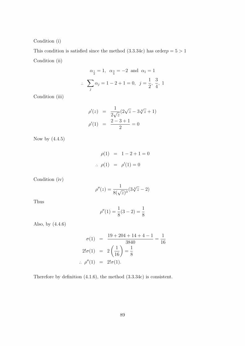
Condition (i)
This condition is satisfied since the method (3.3.34c) has orderp = 5 > 1
Condition (ii)
α 12
= 1, α 34
= −2 and α1 = 1
...∑j
αj = 1− 2 + 1 = 0, j =1
2,
3
4, 1
Condition (iii)
ρ′(z) =1
2√z
(2√z − 3 4
√z + 1)
ρ′(1) =2− 3 + 1
2= 0
Now by (4.4.5)
ρ(1) = 1− 2 + 1 = 0
... ρ(1) = ρ′(1) = 0
Condition (iv)
ρ′′(z) =1
8(√z)3
(3 4√z − 2)
Thus
ρ′′(1) =1
8(3− 2) =
1
8
Also, by (4.4.6)
σ(1) =19 + 204 + 14 + 4− 1
3840=
1
16
2!σ(1) = 2
(1
16
)=
1
8
... ρ′′(1) = 2!σ(1).
Therefore by definition (4.1.6), the method (3.3.34c) is consistent.
89
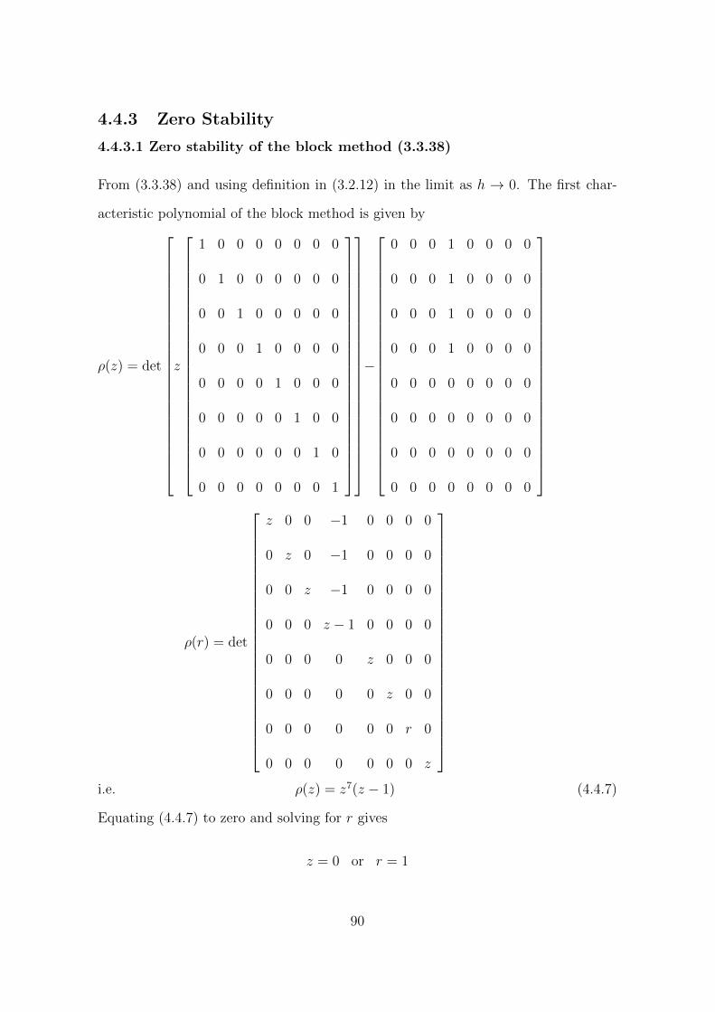
4.4.3 Zero Stability
4.4.3.1 Zero stability of the block method (3.3.38)
From (3.3.38) and using definition in (3.2.12) in the limit as h → 0. The first char-
acteristic polynomial of the block method is given by
ρ(z) = det
z
1 0 0 0 0 0 0 0
0 1 0 0 0 0 0 0
0 0 1 0 0 0 0 0
0 0 0 1 0 0 0 0
0 0 0 0 1 0 0 0
0 0 0 0 0 1 0 0
0 0 0 0 0 0 1 0
0 0 0 0 0 0 0 1
−
0 0 0 1 0 0 0 0
0 0 0 1 0 0 0 0
0 0 0 1 0 0 0 0
0 0 0 1 0 0 0 0
0 0 0 0 0 0 0 0
0 0 0 0 0 0 0 0
0 0 0 0 0 0 0 0
0 0 0 0 0 0 0 0
ρ(r) = det
z 0 0 −1 0 0 0 0
0 z 0 −1 0 0 0 0
0 0 z −1 0 0 0 0
0 0 0 z − 1 0 0 0 0
0 0 0 0 z 0 0 0
0 0 0 0 0 z 0 0
0 0 0 0 0 0 r 0
0 0 0 0 0 0 0 z
i.e. ρ(z) = z7(z − 1) (4.4.7)
Equating (4.4.7) to zero and solving for r gives
z = 0 or r = 1
90
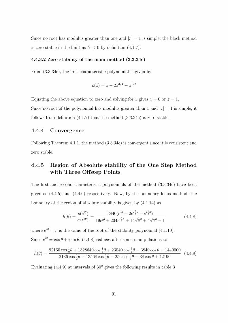
Since no root has modulus greater than one and |r| = 1 is simple, the block method
is zero stable in the limit as h→ 0 by definition (4.1.7).
4.4.3.2 Zero stability of the main method (3.3.34c)
From (3.3.34c), the first characteristic polynomial is given by
ρ(z) = z − 2z3/4 + z1/2
Equating the above equation to zero and solving for z gives z = 0 or z = 1.
Since no root of the polynomial has modulus greater than 1 and |z| = 1 is simple, it
follows from definition (4.1.7) that the method (3.3.34c) is zero stable.
4.4.4 Convergence
Following Theorem 4.1.1, the method (3.3.34c) is convergent since it is consistent and
zero stable.
4.4.5 Region of Absolute stability of the One Step Methodwith Three Offstep Points
The first and second characteristic polynomials of the method (3.3.34c) have been
given as (4.4.5) and (4.4.6) respectively. Now, by the boundary locus method, the
boundary of the region of absolute stability is given by (4.1.14) as
h(θ) =ρ(eiθ)
σ(eiθ)=
3840(eiθ − 2ei34θ + ei
12θ)
19eiθ + 204ei34θ + 14ei
12θ + 4ei
14θ − 1
(4.4.8)
where eiθ = r is the value of the root of the stability polynomial (4.1.10).
Since eiθ = cos θ + i sin θ, (4.4.8) reduces after some manipulations to
h(θ) =92160 cos 1
2θ + 1328640 cos 1
4θ + 23040 cos 3
4θ − 3840 cos θ − 1440000
2136 cos 12θ + 13568 cos 1
4θ − 256 cos 3
4θ − 38 cos θ + 42190
(4.4.9)
Evaluating (4.4.9) at intervals of 300 gives the following results in table 3
91
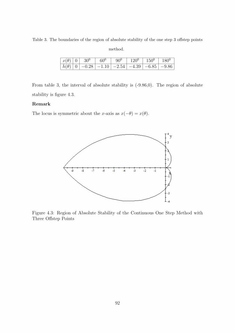
Table 3. The boundaries of the region of absolute stability of the one step 3 offstep points
method.
x(θ) 0 300 600 900 1200 1500 1800
h(θ) 0 −0.28 −1.10 −2.54 −4.39 −6.85 −9.86
From table 3, the interval of absolute stability is (-9.86,0). The region of absolute
stability is figure 4.3.
Remark
The locus is symmetric about the x-axis as x(−θ) = x(θ).
Figure 4.3: Region of Absolute Stability of the Continuous One Step Method withThree Offstep Points
92
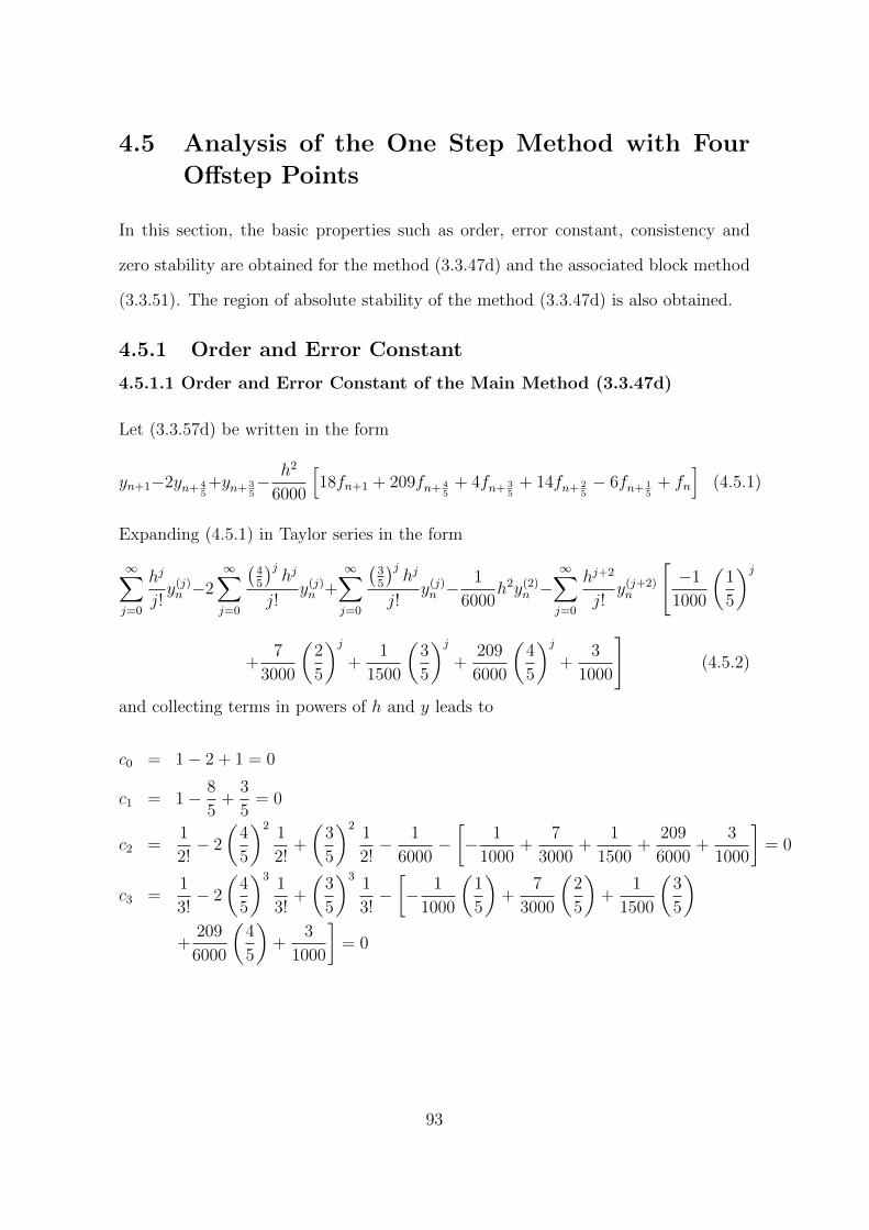
4.5 Analysis of the One Step Method with Four
Offstep Points
In this section, the basic properties such as order, error constant, consistency and
zero stability are obtained for the method (3.3.47d) and the associated block method
(3.3.51). The region of absolute stability of the method (3.3.47d) is also obtained.
4.5.1 Order and Error Constant
4.5.1.1 Order and Error Constant of the Main Method (3.3.47d)
Let (3.3.57d) be written in the form
yn+1−2yn+ 45+yn+ 3
5− h2
6000
[18fn+1 + 209fn+ 4
5+ 4fn+ 3
5+ 14fn+ 2
5− 6fn+ 1
5+ fn
](4.5.1)
Expanding (4.5.1) in Taylor series in the form
∞∑j=0
hj
j!y(j)n −2
∞∑j=0
(45
)jhj
j!y(j)n +
∞∑j=0
(35
)jhj
j!y(j)n −
1
6000h2y(2)n −
∞∑j=0
hj+2
j!y(j+2)n
[−1
1000
(1
5
)j
+7
3000
(2
5
)j+
1
1500
(3
5
)j+
209
6000
(4
5
)j+
3
1000
](4.5.2)
and collecting terms in powers of h and y leads to
c0 = 1− 2 + 1 = 0
c1 = 1− 8
5+
3
5= 0
c2 =1
2!− 2
(4
5
)21
2!+
(3
5
)21
2!− 1
6000−[− 1
1000+
7
3000+
1
1500+
209
6000+
3
1000
]= 0
c3 =1
3!− 2
(4
5
)31
3!+
(3
5
)31
3!−[− 1
1000
(1
5
)+
7
3000
(2
5
)+
1
1500
(3
5
)+
209
6000
(4
5
)+
3
1000
]= 0
93
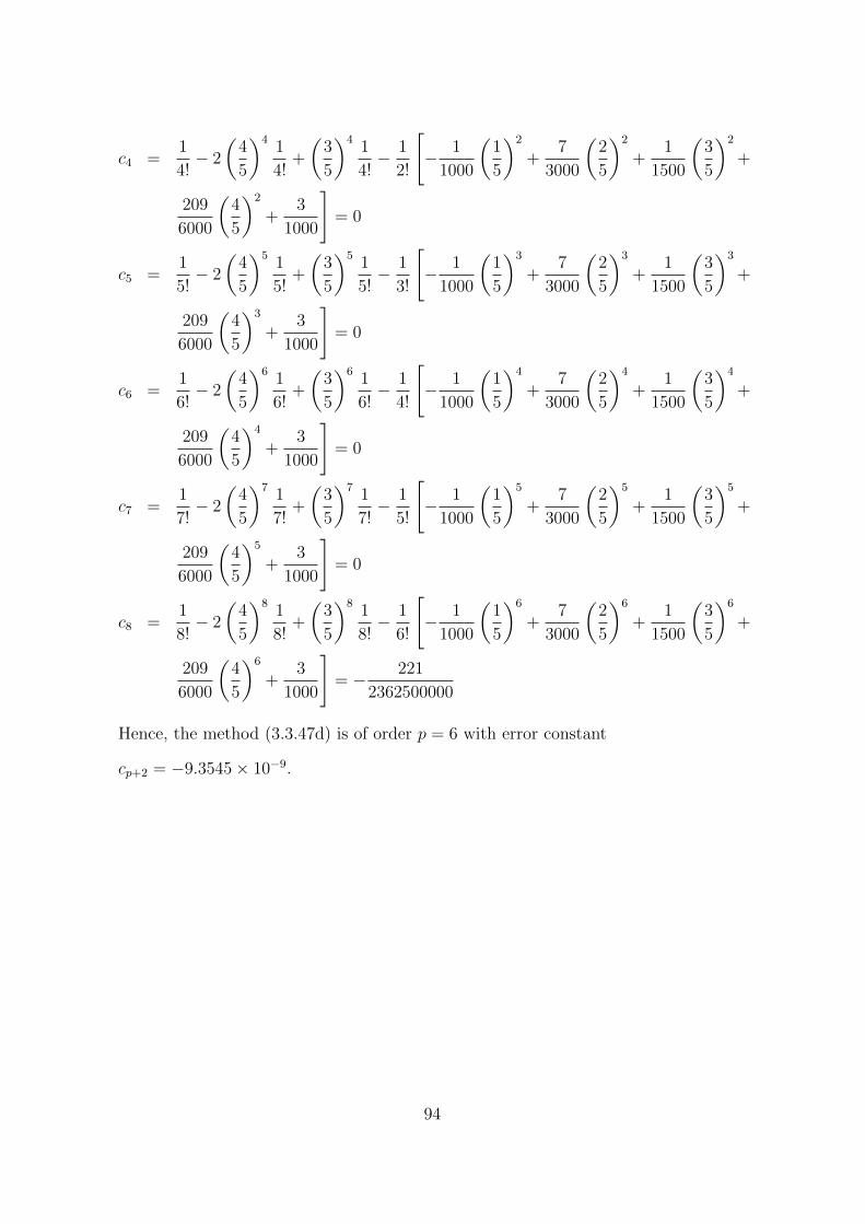
c4 =1
4!− 2
(4
5
)41
4!+
(3
5
)41
4!− 1
2!
[− 1
1000
(1
5
)2
+7
3000
(2
5
)2
+1
1500
(3
5
)2
+
209
6000
(4
5
)2
+3
1000
]= 0
c5 =1
5!− 2
(4
5
)51
5!+
(3
5
)51
5!− 1
3!
[− 1
1000
(1
5
)3
+7
3000
(2
5
)3
+1
1500
(3
5
)3
+
209
6000
(4
5
)3
+3
1000
]= 0
c6 =1
6!− 2
(4
5
)61
6!+
(3
5
)61
6!− 1
4!
[− 1
1000
(1
5
)4
+7
3000
(2
5
)4
+1
1500
(3
5
)4
+
209
6000
(4
5
)4
+3
1000
]= 0
c7 =1
7!− 2
(4
5
)71
7!+
(3
5
)71
7!− 1
5!
[− 1
1000
(1
5
)5
+7
3000
(2
5
)5
+1
1500
(3
5
)5
+
209
6000
(4
5
)5
+3
1000
]= 0
c8 =1
8!− 2
(4
5
)81
8!+
(3
5
)81
8!− 1
6!
[− 1
1000
(1
5
)6
+7
3000
(2
5
)6
+1
1500
(3
5
)6
+
209
6000
(4
5
)6
+3
1000
]= − 221
2362500000
Hence, the method (3.3.47d) is of order p = 6 with error constant
cp+2 = −9.3545× 10⁻⁹.
94

4.5.1.2 Order of the block method (3.3.51)
Let (3.3.51) be expressed in the form
1 0 0 0 0 0 0 0 0 0
0 1 0 0 0 0 0 0 0 0
0 0 1 0 0 0 0 0 0 0
0 0 0 1 0 0 0 0 0 0
0 0 0 0 1 0 0 0 0 0
0 0 0 0 0 1 0 0 0 0
0 0 0 0 0 0 1 0 0 0
0 0 0 0 0 0 0 1 0 0
0 0 0 0 0 0 0 0 1 0
0 0 0 0 0 0 0 0 0 1
yn+ 15
yn+ 25
yn+ 35
yn+ 45
yn+1
y′n+ 1
5
y′n+ 2
5
y′n+ 3
5
y′n+ 4
5
y′n+1
−
1 15h
1 25h
1 35h
1 45h
1 h
0 1
0 1
0 1
0 1
0 1
yn
y′n
−
1231126000
h2
713150
h2
1233500
h2
3767875
h2
611008
h2
19288h
15225h
51800h
14225
19288h
[fn]
−
86350400
h2 − 76163000
h2 941126000
h2 − 341126000
h2 107252000
h2
5447875
h2 − 371575
h2 1367875
h2 − 10115750
h2 87875
h2
350128000
h2 − 93500
h2 872800
h2 − 9875h2 9
5600h2
14247875
h2 1767875
h2 6087875
h2 − 161575
h2 167875
h2
4752016
h2 25504h2 125
1008h 25
1008h2 11
2016h2
14277200
h − 1331200
h 2413600
h − 1737200
h 3800h
43150h 7
225h 7
225h − 1
75h 1
450h
219800h 57
400h 57
400h − 21
800h 3
800h
64225h 8
75h 64
225h 14
225h 0
2596h 25
144h 25
144h 25
96h 19
288h
fn+ 15
fn+ 25
fn+ 35
fn+ 45
fn+1
(4.5.3)
95
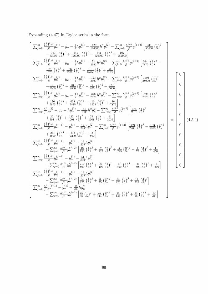
Expanding (4.47) in Taylor series in the form
∑∞j=0
( 15)
jhj
j!y(j)n − yn − 1
5hy
(1)n − 1231
126000h2y
(2)n −
∑∞j=0
hj+2
j!y(j+2)n
[863
50400
(15
)j− 761
63000
(25
)j+ 941
126000
(35
)j − 341126000
(45
)j+ 107
252000
]∑∞
j=0
( 25)
jhj
j!y(j)n − yn − 2
5hy
(1)n − 71
3150h2y
(2)n −
∑∞j=0
hj+2
j!y(j+2)n
[5447875
(15
)j −37
1575
(25
)j+ 136
7875
(35
)j − 10115750
(45)j + 8
7875
]∑∞
j=0
( 35)
jhj
j!y(j)n − yn − 3
5hy
(1)n − 123
3500h2y
(2)n −
∑∞j=0
hj+2
j!y(j+2)n
[350128000
(15
)j− 9
3500
(25
)j+ 87
2800
(35
)j − 9875
(45
)j+ 9
5600
]∑∞
j=0
( 45)
jhj
j!y(j)n − yn − 4
5hy
(1)n − 376
7875h2y
(2)n −
∑∞j=0
hj+2
j!y(j+2)n
[14247875
(15
)j+ 176
7875
(25
)j+ 608
7875
(35
)j − 161575
(45
)j+ 16
7875
]∑∞
j=0hj
j!y(j)n − yn − hy(1)n − 61
1008h2y2n −
∑∞j=0
hj+2
j!y(j+2)n
[4752016
(15
)j+ 25
504
(25
)j+ 125
1008
(35
)j+ 25
1008
(45
)+ 11
2016
]∑∞
j=0
( 15)
jhj
j!y(j+1)n − y(1)n − 19
288hy
(2)n −
∑∞j=0
hj+1
j!y(j+2)n
[14277200
(15
)j − 1331200
(25
)j+ 241
3600
(35
)j − 1737200
(45
)j+ 3
800
]∑∞
j=0
( 25)
jhj
j!y(j+1)n − y(1)n − 14
225hy
(2)n
−∑∞
j=0hj+1
j!y(j+2)n
[43150
(15
)j+ 7
225
(25
)j+ 7
225
(35
)j − 175
(45
)j+ 1
450
]∑∞
j=0
( 35)
jhj
j!y(j+1)n − y(1)n − 51
800hy
(2)n
−∑∞
j=0hj+1
j!y(j+2)n
[219800
(15
)j+ 57
400
(25
)j+ 57
400
(35
)j − 21800
(45
)j+ 3
800
]∑∞
j=0
( 45)
jhj
j!y(j+1)n − y(1)n − 14
225hy
(2)n
−∑∞
j=0hj+1
j!y(j+2)n
[64225
(15
)j+ 8
75
(25
)j+ 64
226
(35
)j+ 14
225
(45
)j]∑∞j=0
hj
j!y(j+1)n − y(1)n − 19
288hy2n
−∑∞
j=0hj+1
j!y(j+2)n
[2596
(15
)j+ 25
144
(25
)j+ 25
144
(35
)j+ 25
96
(45
)j+ 19
288
]
=
0
0
0
0
0
0
0
0
0
0
(4.5.4)
96
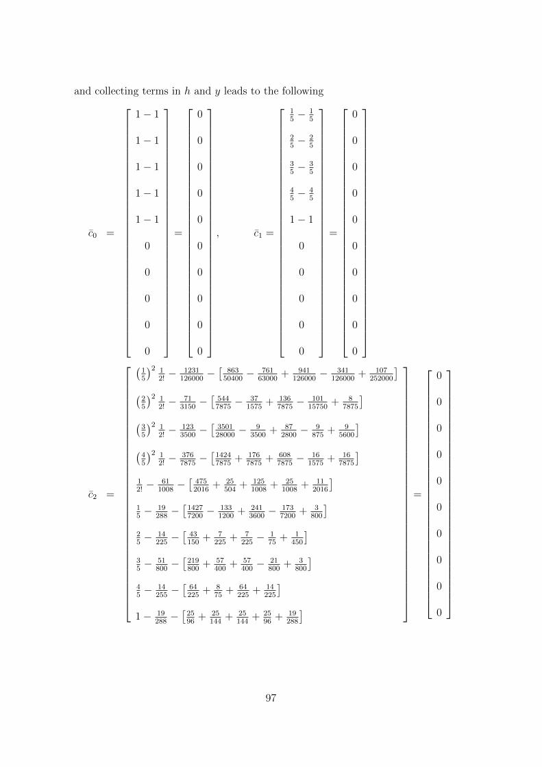
and collecting terms in h and y leads to the following
c0 =
1− 1
1− 1
1− 1
1− 1
1− 1
0
0
0
0
0
=
0
0
0
0
0
0
0
0
0
0
, c1 =
15− 1
5
25− 2
5
35− 3
5
45− 4
5
1− 1
0
0
0
0
0
=
0
0
0
0
0
0
0
0
0
0
c2 =
(15
)2 12!− 1231
126000−[
86350400
− 76163000
+ 941126000
− 341126000
+ 107252000
](25
)2 12!− 71
3150−[
5447875− 37
1575+ 136
7875− 101
15750+ 8
7875
](35
)2 12!− 123
3500−[
350128000
− 93500
+ 872800− 9
875+ 9
5600
](45
)2 12!− 376
7875−[14247875
+ 1767875
+ 6087875− 16
1575+ 16
7875
]12!− 61
1008−[
4752016
+ 25504
+ 1251008
+ 251008
+ 112016
]15− 19
288−[14277200− 133
1200+ 241
3600− 173
7200+ 3
800
]25− 14
225−[
43150
+ 7225
+ 7225− 1
75+ 1
450
]35− 51
800−[219800
+ 57400
+ 57400− 21
800+ 3
800
]45− 14
255−[
64225
+ 875
+ 64225
+ 14225
]1− 19
288−[2596
+ 25144
+ 25144
+ 2596
+ 19288
]
=
0
0
0
0
0
0
0
0
0
0
97
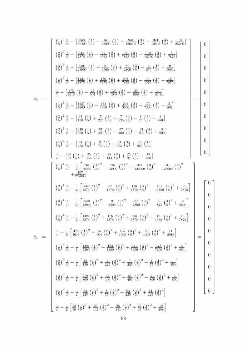
c3 =
(15
)3 13!−[
86350400
(15
)− 761
63000
(25
)+ 941
126000
(35
)− 341
12600
(45
)+ 107
25200
](25
)3 13!−[
5447875
(15
)− 37
1575
(25
)+ 136
7875
(35
)− 101
15750
(45
)+ 8
7875
](35
)3 13!−[
350128000
(15
)− 9
3500
(25
)+ 87
2800
(35
)− 9
875
(45
)+ 9
5600
](45
)3 13!−[14247875
(15
)+ 176
7875
(25
)+ 608
7875
(35
)− 16
1575
(45
)+ 16
7875
]13!−[
4752016
(15
)− 25
504
(25
)+ 125
1008
(35
)− 25
1008
(45
)+ 11
2016
](15
)2 12!−[14277200
(15
)− 133
1200
(25
)+ 241
3600
(35
)− 173
7200
(45
)+ 3
800
](25
)2 12!−[
43150
(15
)+ 7
225
(25
)+ 7
225
(35
)− 1
75
(45
)+ 1
450
](35
)2 12!−[219800
(15
)+ 57
400
(25
)+ 57
400
(35
)− 21
800
(45
)+ 3
800
](45
)2 12!−[
64225
(15
)+ 8
75
(25
)+ 64
225
(35
)+ 14
225
(45
)]12!−[2596
(15
)+ 25
144
(25
)+ 25
144
(35
)+ 25
96
(45
)+ 19
288
]
=
0
0
0
0
0
0
0
0
0
0
c4 =
(15
)4 14!− 1
2!
[761
50400
(15
)2 − 76163000
(25
)2+ 941
126000
(35
)2 − 341126000
(45
)2+ 107
252000
](25
)4 14!− 1
2!
[5447875
(15
)2 − 371575
(25
)2+ 136
7875
(35
)2 − 10115750
(45
)2+ 8
7875
](35
)4 14!− 1
2!
[350128000
(15
)2 − 93500
(25
)2 − 872800
(35
)2 − 9875
(45
)2+ 9
5600
](45
)4 14!− 1
2!
[14247875
(15
)2+ 176
7875
(25
)2+ 608
7875
(35
)2 − 161575
(45
)2+ 16
7875
]14!− 1
2!
[4752016
(15
)2+ 25
504
(25
)2+ 125
1008
(35
)2+ 25
1008
(45
)2+ 11
2016
](15
)3 13!− 1
2!
[14277200
(15
)2 − 1331200
(25
)2+ 241
3600
(35
)2 − 1737200
(45
)2+ 3
800
](25
)3 13!− 1
2!
[43150
(15
)2+ 7
225
(25
)2+ 7
225
(35
)2 − 175
(45
)2+ 1
450
](35
)3 13!− 1
2!
[219800
(15
)2+ 57
400
(25
)2+ 57
400
(35
)2 − 21800
(45
)2+ 3
800
](45
)3 13!− 1
2!
[64225
(15
)2+ 8
75
(25
)2+ 64
225
(35
)2+ 14
225
(45
)2]13!− 1
2!
[2596
(15
)2+ 25
144
(25
)2+ 25
144
(35
)2+ 25
96
(45
)2+ 19
288
]
=
0
0
0
0
0
0
0
0
0
0
98
c5 =
(15
)5 15!− 1
3!
[863
50400
(15
)3 − 76163000
(25
)3+ 941
126000
(35
)3 − 341126000
(45
)3+ 107
252000
](25
)5 15!− 1
3!
[5447875
(15
)3 − 371575
(25
)3+ 136
7875
(35
)3 − 10115750
(45
)3+ 8
7875
](35
)5 15!− 1
3!
[350128000
(15
)3 − 93500
(25
)3+ 87
2800
(35
)3 − 9875
(45
)3+ 9
5600
](45
)5 15!− 1
3!
[14247879
(15
)3+ 176
7875
(25
)3+ 608
7875
(35
)3 − 161575
(45
)3+ 16
7875
]15!− 1
3!
[4752016
(15
)3+ 25
504
(25
)3+ 125
1008
(35
)3+ 25
1008
(45
)3+ 11
2016
](15
)4 14!− 1
3!
[14277200
(15
)3 − 1331200
(25
)3+ 241
3600
(35
)3 − 1737200
(45
)3+ 3
800
](25
)4 14!− 1
3!
[43150
(15
)3+ 7
225
(25
)3+ 7
225
(35
)3 − 175
(45
)3+ 1
450
](35
)4 14!− 1
3!
[219800
(15
)3+ 57
400
(25
)3+ 57
400
(35
)3 − 21800
(45
)3+ 3
800
](45
)4 14!− 1
3!
[64225
(15
)3+ 8
75
(25
)3+ 64
225
(35
)3+ 14
225
(45
)3]14!− 1
3!
[2596
(15
)3+ 25
144
(25
)3+ 25
144
(35
)3+ 25
96
(45
)3+ 19
288
]
=
0
0
0
0
0
0
0
0
0
0
c6 =
(15
)6 16!− 1
4!
[863
50400
(15
)4 − 76163000
(25
)4+ 941
126000
(35
)4 − 341126000
(45
)4+
107252000
](25
)6 16!− 1
4!
[5447875
(15
)4 − 371575
(25
)4+ 136
7875
(35
)4 − 10115750
(45
)4+ 8
7875
](35
)6 16!− 1
4!
[350128000
(15
)4 − 93500
(25
)4+ 87
2800
(35
)4 − 9875
(45
)4+ 9
5600
](45
)6 16!− 1
4!
[14247879
(15
)4+ 176
7875
(25
)4+ 608
7875
(35
)4 − 161575
(45
)4+ 16
7875
]16!− 1
4!
[4752016
(15
)4+ 25
504
(25
)4+ 125
1008
(35
)4+ 25
1008
(45
)4+ 11
2016
](15
)5 15!− 1
4!
[14277200
(15
)4 − 1331200
(25
)4+ 241
3600
(35
)4 − 1737200
(45
)4+ 3
800
](25
)5 15!− 1
4!
[43150
(15
)4+ 7
225
(25
)4+ 7
225
(35
)4 − 175
(45
)4+ 1
450
](35
)5 15!− 1
4!
[219800
(15
)4+ 57
400
(25
)4+ 57
400
(35
)4 − 21800
(45
)4+ 3
800
](45
)5 15!− 1
4!
[64225
(15
)4+ 8
75
(25
)4+ 64
225
(35
)4+ 14
225
(45
)4]15!− 1
4!
[2596
(15
)4+ 25
144
(25
)4+ 25
144
(35
)4+ 25
96
(45
)4+ 19
288
]
=
0
0
0
0
0
0
0
0
0
0
99
c7 =
(15
)7 17!− 1
5!
[863
50400
(15
)5 − 76163000
(25
)5+ 941
126000
(35
)5 − 341126000
(45
)5+ 107
252000
](25
)7 17!− 1
5!
[5447875
(15
)5 − 371575
(25
)5+ 136
7875
(35
)5 − 10115750
(45
)5+ 8
7875
](35
)7 17!− 1
5!
[350128000
(15
)5 − 93500
(25
)5+ 87
2800
(35
)5 − 9875
(45
)5+ 9
5600
](45
)7 17!− 1
5!
[14247879
(15
)5+ 176
7875
(25
)5+ 608
7875
(35
)5 − 161575
(45
)5+ 16
7875
]17!− 1
5!
[4752016
(15
)5+ 25
504
(25
)5+ 125
1008
(35
)5+ 25
1008
(45
)5+ 11
2016
](15
)6 16!− 1
5!
[14277200
(15
)5 − 1331200
(25
)5+ 241
3600
(35
)5 − 1737200
(45
)5+ 3
800
](25
)6 16!− 1
5!
[43150
(15
)5+ 7
225
(25
)5+ 7
225
(35
)5 − 175
(45
)5+ 1
450
](35
)6 16!− 1
5!
[219800
(15
)5+ 57
400
(25
)5+ 57
400
(35
)5 − 21800
(45
)5+ 3
800
](45
)6 16!− 1
5!
[64225
(15
)5+ 8
75
(25
)5+ 64
225
(35
)5+ 14
225
(45
)5]16!− 1
5!
[2596
(15
)5+ 25
144
(25
)5+ 25
144
(35
)5+ 25
96
(45
)5+ 19
288
]
=
0
0
0
0
0
0
0
0
0
0
100

c8 =
(15
)8 18!− 1
6!
[863
50400
(15
)6 − 76163000
(25
)6+ 941
126000
(35
)6 − 341126000
(45
)6+ 107
252000
](25
)8 18!− 1
6!
[5447875
(15
)6 − 371575
(25
)6+ 136
7875
(35
)6 − 10115750
(45
)6+ 8
7875
](35
)8 18!− 1
6!
[350128000
(15
)6 − 93500
(25
)6+ 87
2800
(35
)6 − 9875
(45
)6+ 9
5600
](45
)8 18!− 1
6!
[14247875
(15
)6+ 176
7875
(25
)6+ 608
7875
(35
)6 − 161575
(45
)6+ 16
7875
]18!− 1
6!
[4752016
(15
)6+ 25
504
(25
)6+ 125
1008
(35
)6+ 25
1008
(45
)6+ 11
2016
](15
)7 17!− 1
6!
[14277200
(15
)6 − 1331200
(25
)6+ 241
3600
(35
)6 − 1737200
(45
)6+ 3
800
](25
)7 17!− 1
6!
[43150
(15
)6+ 7
225
(25
)6+ 7
225
(35
)6 − 175
(45
)6+ 1
450
](35
)7 17!− 1
6!
[219800
(15
)6+ 57
400
(25
)6+ 57
400
(35
)6 − 21800
(45
)6+ 3
800
](45
)7 17!− 1
6!
[64225
(15
)6+ 8
75
(25
)6+ 64
225
(35
)6+ 14
225
(45
)6]17!− 1
6!
[2596
(15
)6+ 25
144
(25
)6+ 25
144
(35
)6+ 25
96
(45
)6+ 19
288
]
=
− 1999450000000
− 19369140625
− 1411750000000
− 873828125
− 1175600000
− 8634725000000
− 37295312500
− 29175000000
− 873828125
− 1137800000
Hence the block method (3.3.51) is of order p = (6, 6, 6, 6, 6, 6, 6, 6, 6, 6)T with error
constant cp+2 =(− 199
4950000000, − 19
369140625, − 141
1750000000, − 8
73828125, − 11
75600000, − 863
4725000000,
− 37295312500
, − 29175000000
, − 873828125
, − 1137800000
)T.
4.5.2 Consistency
The block method (3.3.51) has order p = (6, 6, 6, 6, 6, 6, 6, 6, 6, 6)T > 1, therefore, by
condition (i) in definition (4.1.6) it is consistent. Following the consistency of the
block method (3.3.51), the consistency of method (3.3.47d) is shown as follows by
conditions (i) - (iv) in definition (4.1.6).
Condition (i)
The main method (3.3.47d) is of order p = 6 > 1, which satisfies condition (i) of
101

definition (4.1.6).
Condition (ii)
The first and second characteristic polynomials of method (3.3.47d) are given respec-
tively by
ρ(z) = z − 2z4/5 + z3.5 (4.5.5)
and
σ(z) =18z + 209z4/5 + 4z3/5 + 14z2/5 − 6z1/5 + 1
6000(4.5.6)
From (4.5.5), α3/5 = 1, α4/5 = −2 and α1 = 1 therefore∑j
αj = 1− 2 + 1 = 0, j =3
5,
4
5, 1
Condition (iii)
From (4.5.5),
ρ′(z) =1
5z−2/5(5z2/5 − 8z1/5 + 3)
⇒ ρ′(1) = 15(5− 8 + 3) = 0
(4.5.7)
Also by (4.5.5)
ρ(1) = 1− 2 + 1 = 0
ρ(1) = ρ′(1) = 0
Condition (iv)
From (4.5.7),
ρ′′(z) =2
25z−7/5(4z1/5 − 3)
=2
25(4− 3) =
2
25
From (4.5.6),
σ(1) =18 + 209 + 4 + 14− 6 + 1
6000=
1
25
⇒ 2!σ(1) = 2
(1
25
)=
2
25
... ρ′′(1) = 2!σ(1)
102

Thus by definition (4.1.6), the main method (3.3.47d) is consistent.
4.5.3 Zero Stability of the One Step Method with Four Off-step Points
4.5.3.1 Zero stability of the Block Method (3.3.51)
Using (3.3.51) and (3.2.12) in the limit as h → 0 in (4.1.9), the first characteristic
polynomial of the block method is obtained (by equation (4.1.9)) as
ρ(z) = det
z
1 0 0 0 0 0 0 0 0 0
0 1 0 0 0 0 0 0 0 0
0 0 1 0 0 0 0 0 0 0
0 0 0 1 0 0 0 0 0 0
0 0 0 0 1 0 0 0 0 0
0 0 0 0 0 1 0 0 0 0
0 0 0 0 0 0 1 0 0 0
0 0 0 0 0 0 0 1 0 0
0 0 0 0 0 0 0 0 1 0
0 0 0 0 0 0 0 0 0 1
−
0 0 0 0 1 0 0 0 0 0
0 0 0 0 1 0 0 0 0 0
0 0 0 0 1 0 0 0 0 0
0 0 0 0 1 0 0 0 0 0
0 0 0 0 1 0 0 0 0 0
0 0 0 0 0 0 0 0 0 0
0 0 0 0 0 0 0 0 0 0
0 0 0 0 0 0 0 0 0 0
0 0 0 0 0 0 0 0 0 0
0 0 0 0 0 0 0 0 0 0
103

i.e.
ρ(r) = det
z 0 0 0 −1 0 0 0 0 0
0 z 0 0 −1 0 0 0 0 0
0 0 z 0 −1 0 0 0 0 0
0 0 0 z −1 0 0 0 0 0
0 0 0 0 z − 1 0 0 0 0 0
0 0 0 0 0 z 0 0 0 0
0 0 0 0 0 0 z 0 0 0
0 0 0 0 0 0 0 z 0 0
0 0 0 0 0 0 0 0 z 0
0 0 0 0 0 0 0 0 0 z
= z10 − z9 (4.5.8)
Equating (4.5.8) to zero and solving for z gives z = 0 or 1.
Since no root has modulus greater than one and |z| = 1 is simple, the block method
is zero stable in the limit as h→ 0 by definition (4.1.8).
4.5.3.2 Zero Stability of the Main Method (3.3.47d)
Equation (4.5.5) is the first characteristic polynomial of the main method (3.3.47d).
Equating (4.5.5) to zero and solving for z gives z = 0 or z = 1.
We can see that no root has modulus greater than one and |z| = 1 is simple. It
follows from definition (4.1.7) that the method is zero stable.
4.5.4 Convergence
Convergence of the main method (3.3.47d) follows from Theorem 4.1.1.
104

4.5.5 Region of absolute stability of the One step methodwith four offstep points
The first and second characteristics polynomials of the main method (3.3.47d) were
given as (4.5.5) and (4.5.6) respectively. Hence, by the boundary locus method, the
boundary of the region of absolute stability is given by (4.1.14) where z = eiθ as
h(θ) =ρ(eiθ)
σ(eiθ)=
6000(eiθ − 2ei45θ + ei
35θ)
18eiθ + 209ei45θ + 4ei
35θ + 14ei
25θ − 6ei
15θ + 1
(4.5.9)
where eiθ = z is the value of the root of the stability polynomial (4.1.10). Recall that
eiθ = cos θ + i sin θ, thus (4.53) reduces to
h(θ) =2328000 cos 1
5θ − 72000 cos 2
5θ + 162000 cos 3
5θ − 48000 cos 4
5θ + 6000 cos θ − 2376000
9128 cos 15θ + 5976 cos 2
5θ − 1996 cos 3
5θ + 202 cos 4
5θ + 36 cos θ + 44254
(4.5.10)
Evaluating (4.5.10) at intervals of 300 gives the results in table 4.
Table 4. The boundaries of the region of absolute stability of the one step 4 offstep points
method.
θ 0 300 600 900 1200 1500 1800
h(θ) 0 −0.27 −1.10 −2.47 −6.04 −6.85 −9.87
From table 4, the interval of absolute stability is (−9.87, 0). The region of absolute
stability is shown in figure 4.4.
Remark
The locus is symmetric about x-axis that is x(−θ) = x(θ). Similarly, y(−θ) = y(θ).
105

Figure 4.4: Region of Absolute Stability of the Continuous One Step Method withFour Offstep Points
4.6 Analysis of the One Step Method with Five
Offstep Points
The basic properties of the main method (3.3.60e) such as order, error constant,
consistency and zero stability as well as those of the associated block method (3.3.64)
are obtained in this section. The region of absolute stability of the main method
(3.3.60e) is also obtained here.
4.6.1 Order and Error Constant
4.6.1.1 Order and error constant of the main method (3.3.60e)
Let (3.3.60e) be written in the form
yn+1 − 2yn+ 56− yn+ 2
3− h
2177280
[4315fn+1 + 53994fn+ 5
6− 2307fn+ 2
3
+7948fn+ 12− 4827fn+ 1
3+ 1578fn+ 1
6− 221fn
](4.5.11)
106
Expanding in Taylor series in the form
∞∑j=1
hj
j!y(j)n − 2
∞∑j=0
(56
)jhj
j!y(j)n +
∞∑j=0
(23
)jhj
j!y(j)n +
221
2177280h2y(1)n −
∞∑j=0
hj+2
j!yj+2n
(1
6
)j[
263
362880− 1609
725760
(1
3
)j+
1987
544320
(1
2
)j− 769
725760
(2
3
)j+
8999
362880
(5
6
)j+
863
435456
](4.5.12)
and collecting terms in powers of h and y leads to the following:
c0 = 1− 2 + 1 = 0
c1 = 1− 2
(5
6
)+
2
3= 0
c2 =1
2!− 2
(5
6
)21
2!+
(2
3
)21
2!+
221
2177280−[
263
362880− 1609
725760+
1987
544320− 769
725760
+8999
362880+
863
435456
]= 0
c3 =1
3!− 2
(5
6
)31
3!+
(2
3
)31
3!−[
263
362880
(1
6
)− 1609
725760
(1
3
)+
1987
544320
(1
2
)− 769
725760
(2
3
)+
8999
362880
(5
6
)+
863
435456
]= 0
c4 =1
4!− 2
(5
6
)41
4!+
(2
3
)41
4!− 1
2!
[263
362880
(1
6
)2
− 1609
725760
(1
3
)2
+1987
544320
(1
2
)2
− 769
725760
(2
3
)2
+8999
362880
(5
6
)+
863
435456
]= 0
107
c5 =1
5!− 2
(5
6
)51
5!+
(2
5
)51
5!− 1
3
[263
362880
(1
6
)2
− 1609
725760
(1
3
)3
+1987
544320
(1
2
)3
− 769
725760
(2
3
)3
+8999
362880
(5
6
)3
+863
435456
]= 0
c6 =1
6!− 2
(5
6
)61
6!+
(2
3
)61
6!− 1
4!
[263
362880
(1
6
)4
− 1609
725760
(1
3
)4
+1987
544320
(1
2
)4
− 769
725760
(2
3
)4
+8999
362880
4
+863
435456
]= 0
c7 =1
7!− 2
(5
6
)71
7!+
(2
3
)71
7!− 1
5!
[263
362880
(1
6
)5
− 1609
725760
(1
3
)5
+1987
544320
(1
2
)5
− 769
725760
(2
3
)5
+8999
362880
(5
6
)5
+863
435456
]= 0
c8 =1
8!− 2
(5
6
)81
8!+
(2
3
)81
8!− 1
6!
[263
362880
(1
6
)6
− 1609
725760
(1
3
)6
+1987
544320
(1
2
)6
− 769
725760
(2
3
)6
+8999
362880
(5
6
)6
+863
435456
]= 0
c9 =1
9!− 2
(5
6
)91
9!+
(2
3
)91
9!− 1
7!
[263
362880
(1
6
)7
− 1609
725760
(1
3
)7
+1987
544320
(1
2
)7
− 769
725760
(2
3
)7
+8999
362880
(5
6
)7
+863
435456
]=
−19
60949905408
Hence, the main method (3.3.60e) has order p = 7 with error constant cp+2 =
−3.1173× 10⁻¹⁰.
108

4.6.1.2 Order of the Block Method (3.3.64)
Let (3.3.64) be expressed in the form
1 0 0 0 0 0 0 0 0 0 0 0
0 1 0 0 0 0 0 0 0 0 0 0
0 0 1 0 0 0 0 0 0 0 0 0
0 0 0 1 0 0 0 0 0 0 0 0
0 0 0 0 1 0 0 0 0 0 0 0
0 0 0 0 0 1 0 0 0 0 0 0
0 0 0 0 0 0 1 0 0 0 0 0
0 0 0 0 0 0 0 1 0 0 0 0
0 0 0 0 0 0 0 0 1 0 0 0
0 0 0 0 0 0 0 0 0 1 0 0
0 0 0 0 0 0 0 0 0 0 1 0
0 0 0 0 0 0 0 0 0 0 0 1
yn+ 16
yn+ 13
yn+ 12
yn+ 23
yn+ 56
yn+1
y′n+ 1
6
y′n+ 1
3
y′n+ 1
2
y′n+ 2
3
y′n+ 5
6
y′n+1
−
1 16h
1 13h
1 12h
1 23h
1 56h
1 h
0 1
0 1
0 1
0 1
0 1
0 1
yn
y′n
−
285494354560
h2
102768040
h2
25310752
h2
2728505
h2
35225870912
h2
41840h2
19087362880
h
113922680
h
1372688
1432835
h
371572576
h
41840h
[fn]
109

−
27520736
h2 − 5717483840
h2 106211088640
h2 − 77031451520
h2 403241920
h2 − 199870912
h2
971890
h2 − 281h2 197
8505h2 − 97
7560h2 23
5670h2 − 19
34020h2
1651792
h2 − 26717920
h2 5128h2 − 363
17920h2 57
8960h2 − 47
53760h2
3762835
h2 − 2945h2 656
8505h2 − 2
81h2 8
945h2 − 2
1701h2
837548384
h2 3125290304
h2 25625217728
h2 − 62596768
h2 27520736
h2 − 1375870912
h2
314h2 3
140h2 17
105h2 3
280h2 3
70h2 0
271315120
h − 15487120960
h 2932835
h − 6737120960
h 26315120
h − 863362880
h
47189h 11
7560h 166
2835h − 269
7560h 11
945h − 37
22680h
27112h 387
4480h 17
105h − 243
4480h 9
560h − 29
13440h
232945h 64
945h 752
2835h 29
945h 8
945h − 4
2835h
7253024
h 212524192
h 125567h 3875
24192h 235
3024h − 275
72576h
935h 9
280h 34
105h 9
280h 9
35h 41
840h
fn+ 16
fn+ 13
fn+ 12
fn+ 23
fn+ 56
fn+1
(4.5.13)
110

Expanding (4.5.13) in Taylor series in the form
∑∞j=0
( 16)
jhj
j!y(j)n − yn − 1
6hy
(1)n − 28549
4354560h2y
(2)n −
∑∞j=0
hj+2
j!y(j+2)n
[275
20736
(16
)j− 5717
483840
(13
)j+ 10621
1088640
(12
)j − 77031451520
(23
)j+ 403
241920
(56
)− 199
870912
]∑∞
j=0
( 13)
jhj
j!y(j)n − yn − 1
3hy
(1)n − 1027
68040h2y
(2)n −
∑∞j=0
hj+2
j!y(j+2)n
[97
1890
(16
)j− 2
81
(13
)j+ 197
8505
(12
)j − 977560
(23
)j+ 23
5670
(56
)j − 1934020
]∑∞
j=0
( 12)
jhj
j!y(j)n − yn − 1
2hy
(1)n − 253
10752h2y
(2)n −
∑∞j=0
hj+2
j!y(j+2)n
[1651792
(16
)j− 267
17920
(13
)j+ 5
128
(12
)j − 36317920
(23
)j+ 57
8960
(56
)j − 4753760
]∑∞
j=0
( 23)
jhj
j!y(j)n − yn − 2
3hy
(1)n − 272
8505h2y
(2)n −
∑∞j=0
hj+2
j!y(j+2)n
[3762835
(16
)j− 2
945
(13
)j+ 656
8505
(12
)j − 281
(23
)j+ 8
945
(56
)j − 21701
]∑∞
j=0
( 56)
jhj
j!y(j)n − yn − 5
6hy
(1)n − 35225
870912h2y
(2)n −
∑∞j=0
hj+2
j!y(j+2)n
[837548384
(16
)j+ 3125
290304
(13
)j+ 25625
217728
(12
)j − 62596768
(23
)j+ 275
20736
(56
)− 1375
870912
]∑∞
j=0hj
j!y(j)n − yn − hy(1)n − 41
840h2y2n −
∑∞j=0
hj+2
j!y(j+2)n
[314
(16
)j+ 3
140
(13
)j+ 17
105
(12
)j+ 3
280
(23
)+ 3
70
(56
)j]∑∞
j=0
( 16)
jhj
j!y(j+1)n − y(1)n − 19087
362880hy
(2)n −
∑∞j=0
hj+1
j!y(j+2)n
[271315120
(16
)j− 15487
120960
(13
)j+ 293
2835
(12
)j − 6737120960
(23
)+ 263
15120
(56
)j − 863362880
]∑∞
j=0
( 13)
jhj
j!y(j+1)n − y(1)n − 1139
22680hy
(2)n −
∑∞j=0
hj+1
j!y(j+2)n
[47189
(16
)j+ 11
7560
(13
)j+ 166
2835
(12
)j − 2697560
(23
)j+ 11
945
(56
)j − 3722680
]∑∞
j=0
( 12)
jhj
j!y(j+1)n − y(1)n − 137
2688hy
(2)n −
∑∞j=0
hj+1
j!y(j+2)n
[27112
(16
)j− 387
4480
(13
)j+ 17
105
(12
)j − 2434480
(23
)j+ 9
560
(56
)j − 2913440
]∑∞
j=0
( 23)
jhj
j!y(j+1)n − y(1)n − 143
2835hy
(2)n −
∑∞j=0
hj+1
j!y(j+2)n
[232945
(16
)j+
64945
(13
)j+ 752
2835
(12
)j+ 29
945
(23
)+ 8
945
(56
)j − 42835
]∑∞
j=0
( 56)
jhj
j!y(j+1)n − y(1)n − 3715
72576hy2n −
∑∞j=0
hj+1
j!y(j+2)n
[7253024
(16
)j+ 2125
24192
(13
)j+ 125
567
(12
)j+ 3875
24192
(23
)j+ 235
3024
(56
)j − 27572576
]∑∞
j=0hj
j!y(j+1)n − y(1)n − 41
840hy
(2)n −
∑∞j=0
hj+1
j!y(j+2)n
[935
(16
)j+ 9
280
(13
)j+ 34
105
(12
)j+ 9
280
(23
)j+ 9
35
(56
)j+ 41
840
]
=
0
0
0
0
0
0
0
0
0
0
0
0
(4.5.14)
111
and collecting terms in powers of h and y leads to
c0 =
1− 1
1− 1
1− 1
1− 1
1− 1
1− 1
0
0
0
0
0
0
=
0
0
0
0
0
0
0
0
0
0
0
0
, c1 =
16− 1
6
13− 1
3
12− 1
2
23− 2
3
56− 5
6
1− 1
1− 1
1− 1
1− 1
1− 1
1− 1
1− 1
=
0
0
0
0
0
0
0
0
0
0
0
0
112

c2 =
(16
)2 12!− 28549
4354560−[
27520736
− 5717483840
+ 106211088640
− 77031451520
+ 403241920
− 199870912
](13
)2 12!− 1027
6804−[
971890− 2
81+ 197
8505− 97
7560+ 23
5670− 19
34020
](12
)2 12!− 253
10752−[
1651792− 267
17920+ 5
128− 363
17920+ 57
8960− 47
53760
](23
)2 12!− 272
8505−[
3762835− 2
945+ 656
8505− 2
81+ 8
945− 2
1701
](56
)2 12!− 35225
870912−[
837548384
+ 3125290304
+ 25625217728
− 62596768
+ 27520736
− 1375870912
]12!− 41
840−[
314
+ 3140
+ 17105
+ 3280
+ 370
]16− 19087
362880−[
271315120
− 15487120960
+ 2932835− 6737
120960+ 263
15120− 863
362880
]13− 1139
22680−[
47189
+ 117560
+ 1662835− 269
7560+ 11
945− 37
22680
]12− 137
2688−[
27112
+ 3874480
+ 17105− 243
4480+ 9
560− 29
13440
]23− 143
2835−[232945
+ 64945
+ 7522835
+ 29945
+ 8945− 4
2835
]56− 3715
72576−[
7253024
+ 212524192
+ 125567
+ 387524192
+ 2353024− 275
72576
]1− 41
840−[
935
+ 9280
+ 34105
+ 9280
+ 935
+ 41840
]
=
0
0
0
0
0
0
0
0
0
0
0
0
113
c3 =
(16
)3 13!−[
27520796
(16
)− 5717
483840
(13
)+ 10621
1088640
(12
)− 7703
1451520
(23
)+ 403
241920
(56
)− 199
870912
](13
)3 13!−[
971890
(16
)− 2
81
(13
)+ 197
8505
(12
)− 97
7560
(23
)+ 26
5670
(56
)− 19
34020
](12
)3 13!−[
1651792
(16
)− 267
17920
(13
)+ 5
128
(12
)− 363
17920
(23
)+ 57
8960
(56
)− 47
53760
](23
)3 13!−[
3762835
(16
)− 2
945
(13
)+ 656
8505
(12
)− 2
81
(23
)+ 8
945
(56
)− 2
1701
](56
)3 13!−[
837548384
(16
)+ 3125
290304
(13
)+ 25625
217728
(12
)− 625
96768
(23
)+ 275
20736
(56
)− 1375
870912
]13!−[
314
(16
)+ 3
140
(13
)+ 17
105
(12
)+ 3
280
(23
)+ 3
70
(56
)](16
)2 12!−[
271315120
(16
)− 15487
120960
(13
)+ 293
2835
(12
)− 6737
120960
(23
)+ 263
15120
(56
)− 863
362880
](13
)2 12!−[
47189
(16
)+ 11
7560
(13
)+ 166
2835
(12
)− 269
7560
(23
)+ 11
945
(56
)− 37
22680
](12
)2 12!−[
27112
(16
)− 387
4480
(13
)+ 17
105
(12
)− 243
4480
(23
)+ 9
560
(56
)− 29
13440
](23
)2 12!−[232945
(16
)+ 64
945
(13
)+ 752
2835
(12
)−+ 29
945
(23
)+ 98
945
(56
)− 4
2835
](56
)2 13!−[
7253024
(16
)+ 2125
24192
(13
)+ 125
567
(12
)+ 3875
24192
(23
)+ 235
3024
(56
)− 275
72576
]12!−[
935
(16
)+ 9
280
(13
)+ 34
105
(12
)+ 9
280
(23
)+ 9
35
(56
)+ 41
840
]
=
0
0
0
0
0
0
0
0
0
0
114

c4 =
(16
)4 14!− 1
2!
[275
20736
(16
)2 − 5717483840
(13
)2+ 10621
1088640
(12
)2 − 77031451520
(23
)2+ 403
241920
(56
)2 − 199870912
](13
)4 14!− 1
2!
[97
1890
(16
)2 − 281
(13
)2+ 197
8505
(12
)2 − 977560
(23
)2+ 26
5670
(56
)2 − 1934020
](12
)4 14!− 1
2!
[1651792
(16
)2 − 26717920
(13
)2+ 5
128
(12
)2 − 36317920
(23
)2+ 57
8960
(56
)2 − 4753760
](23
)4 14!− 1
2!
[3762835
(16
)2 − 2945
(13
)2+ 656
8505
(12
)2 − 281
(23
)2+ 8
945
(56
)2 − 21701
](56
)4 14!− 1
2!
[837548384
(16
)2+ 3125
290304
(13
)2+ 25625
217728
(12
)2 − 62596768
(23
)2+ 275
20736
(56
)2 − 1375870912
]14!− 1
2!
[314
(16
)2+ 3
140
(13
)2+ 17
105
(12
)2+ 3
280
(23
)2+ 3
70
(56
)2](16
)3 13!− 1
2!
[271315120
(16
)2 − 15487120960
(13
)2+ 293
2835
(12
)2 − 6737120960
(23
)2+263
150
(56
)2 − 863362880
](13
)3 13!− 1
2!
[47189
(16
)2+ 11
7560
(13
)2+ 166
2835
(12
)2 − 2697560
(23
)2+ 11
945
(56
)2 − 3722680
](12
)3 13!− 1
2!
[27112
(16
)2+ 387
4480
(13
)2+ 17
105
(12
)2 − 2434480
(23
)2+ 9
560
(56
)2 − 2913440
](23
)3 13!− 1
2!
[232945
(16
)2+ 64
945
(13
)2+ 752
2835
(12
)2+ 29
945
(23
)2+ 8
945
(56
)2 − 42835
](56
)3 13!− 1
2!
[7253024
(16
)2+ 2125
24192
(13
)2+ 125
567
(12
)2+ 3875
24192
(23
)2+ 235
3024
(56
)2 − 27572576
]13!− 1
2!
[935
(16
)2+ 9
280
(13
)2+ 34
105
(12
)2+ 9
280
(23
)2+ 9
35
(56
)2 − 41840
]
=
0
0
0
0
0
0
0
0
0
0
0
0
115

c5 =
(16
)5 15!− 1
3!
[275
20736
(16
)3 − 5717483840
(13
)3+ 10621
1088640
(12
)3 − 77031451520
(23
)3+ 403
241920
(56
)3 − 199870912
](13
)5 15!− 1
3!
[97
1890
(16
)3 − 281
(13
)3+ 197
8505
(12
)3 − 977560
(23
)3+ 23
5670
(56
)3 − 1934020
](12
)5 15!− 1
3!
[1651792
(16
)3 − 26717920
(13
)3+ 5
128
(12
)3 − 36317920
(23
)3+ 57
8960
(56
)3 − 4753760
](23
)5 15!− 1
3!
[3762835
(16
)3 − 2945
(13
)3+ 656
8505
(12
)2 − 281
(23
)3+ 8
945
(56
)3 − 21701
](56
)5 15!− 1
3!
[837548384
(16
)3+ 3125
290304
(13
)3+ 25625
217728
(12
)3 − 62596768
(23
)3+ 275
20736
(56
)2 − 1375870912
]15!− 1
3!
[314
(16
)3+ 3
140
(13
)3+ 17
105
(12
)3+ 3
280
(23
)3+ 3
70
(56
)3](16
)4 14!− 1
3!
[271315120
(16
)3 − 15487120960
(13
)3+ 293
2835
(12
)3 − 6737120960
(23
)3+ 265
15120
(56
)3 − 863362880
](13
)4 14!− 1
3!
[47189
(16
)3+ 11
7560
(13
)3+ 166
2835
(12
)3 − 2697560
(23
)3+ 11
945
(56
)3 − 3722680
](12
)4 14!− 1
3!
[27112
(16
)3+ 387
4480
(13
)3+ 17
105
(12
)3 − 2434480
(23
)3+ 9
560
(56
)3 − 2913440
](23
)4 14!− 1
3!
[232945
(16
)3+ 64
945
(13
)3+ 752
2835
(12
)3 − 29945
(23
)3+ 8
945
(56
)3 − 42835
](56
)4 14!− 1
3!
[7253024
(16
)3+ 2125
24192
(13
)3+ 125
567
(12
)3+ 3875
24192
(23
)3+ 235
3024
(56
)3 − 27572576
]14!− 1
3!
[935
(16
)3+ 9
280
(13
)3+ 34
105
(12
)3+ 9
280
(23
)3+ 9
354
(56
)3 − 41840
]
=
0
0
0
0
0
0
0
0
0
0
0
0
116
c6 =
(16
)6 16!− 1
4!
[275
20736
(16
)4 − 5717483840
(13
)3+ 10621
1088640
(12
)3 − 77031451520
(23
)3+ 403
241920
(56
)3 − 199870912
](13
)6 16!− 1
4!
[97
1890
(16
)4 − 281
(13
)4+ 197
8505
(12
)4 − 977560
(23
)4+ 23
5670
(56
)4 − 1934020
](12
)6 16!− 1
4!
[1651792
(16
)4 − 26717920
(13
)4+ 5
128
(12
)4 − 36317920
(23
)4+ 57
8960
(56
)4 − 4753760
](23
)6 16!− 1
4!
[3762835
(16
)4 − 2945
(13
)4+ 656
8505
(12
)4 − 281
(23
)4+ 8
945
(56
)4 − 21701
](56
)6 16!− 1
4!
[837548384
(16
)4+ 3125
290304
(13
)4+ 25625
217728
(12
)4 − 62596768
(23
)4+ 275
20736
(56
)4 − 1375870912
]16!− 1
4!
[314
(16
)4+ 3
140
(13
)4+ 17
105
(12
)4+ 3
280
(23
)4+ 3
70
(56
)4](16
)5 15!− 1
4!
[271315120
(16
)4 − 15487120960
(13
)4+ 293
2835
(12
)4 − 6737120960
(23
)4+ 265
15120
(56
)4 − 863362880
](13
)5 15!− 1
4!
[47189
(16
)4+ 11
7560
(13
)4+ 166
2835
(12
)4 − 2697560
(23
)4+ 11
945
(56
)4 − 3722680
](12
)5 15!− 1
4!
[27112
(16
)4+ 387
4480
(13
)4+ 17
105
(12
)4 − 2434480
(23
)4+ 9
560
(56
)4 − 2913440
](23
)5 15!− 1
4!
[232945
(16
)4+ 64
945
(13
)4+ 752
2835
(12
)4+ 29
945
(23
)4+ 8
945
(56
)4 − 42835
](56
)5 15!− 1
4!
[7253024
(16
)4+ 2125
24192
(13
)4+ 125
567
(12
)4+ 3875
24192
(23
)4+ 235
3024
(56
)4 − 27572576
]15!− 1
4!
[935
(16
)4+ 9
280
(13
)4+ 34
105
(12
)4+ 9
280
(23
)4+ 9
35
(56
)4 − 41840
]
=
0
0
0
0
0
0
0
0
0
0
0
0
117

c7 =
(16
)7 17!− 1
5!
[275
20736
(16
)5 − 5717483840
(13
)5+ 10621
1088640
(12
)5 − 77031451520
(23
)5+
403241920
(56
)5 − 199870912
](13
)7 17!− 1
5!
[97
1890
(16
)5 − 281
(13
)5+ 197
8505
(12
)5 − 977560
(23
)5+ 23
5670
(56
)5− 19
34020
](12
)7 17!− 1
5!
[1651792
(16
)5 − 26717920
(13
)5+ 5
128
(12
)5 − 36317920
(23
)5+ 57
8960
(56
)5− 47
53760
](23
)7 17!− 1
5!
[376
48384
(16
)5 − 2945
(13
)5+ 656
8505
(12
)5 − 281
(23
)5+ 8
945
(56
)5− 2
1701
](56
)7 17!− 1
5!
[837548384
(16
)5+ 3125
290304
(13
)5+ 25625
217728
(12
)5 − 62596768
(23
)5+
27520736
(56
)5 − 1375870912
]17!− 1
5!
[314
(16
)5+ 3
140
(13
)5+ 17
105
(12
)5+ 3
280
(23
)5+ 3
70
(56
)5](16
)6 16!− 1
5!
[271315120
(16
)5 − 15487120960
(13
)5+ 293
2835
(12
)5 − 6737120960
(23
)5+
26515120
(56
)5 − 863362880
](13
)6 16!− 1
5!
[47189
(16
)5+ 11
7560
(13
)5+ 166
2835
(12
)5 − 2697560
(23
)5+ 11
945
(56
)5− 37
22680
](12
)6 16!− 1
5!
[27112
(16
)5+ 387
4480
(13
)5+ 17
105
(12
)5 − 2434480
(23
)5+ 9
560
(56
)5− 29
13440
](23
)6 16!− 1
5!
[232945
(16
)5+ 64
945
(13
)5+ 752
2835
(12
)5+ 29
945
(23
)5+ 8
945
(56
)5− 4
2835
](56
)6 16!− 1
5!
[7253024
(16
)5+ 2125
24192
(13
)5+ 125
567
(12
)5+ 3875
24192
(23
)5+ 235
3024
(56
)5− 275
72576
]16!− 1
5!
[935
(16
)5+ 9
280
(13
)5+ 34
105
(12
)5+ 9
280
(23
)5+ 9
35
(56
)5 − 41840
]
=
0
0
0
0
0
0
0
0
0
0
0
0
118
c8 =
(16
)8 18!− 1
6!
[275
20736
(16
)6 − 5717483840
(13
)6+ 10621
1088640
(12
)6 − 77031451520
(23
)6+ 403
241920
(56
)6 − 199870912
](13
)8 18!− 1
6!
[97
1890
(16
)6 − 281
(13
)6+ 197
8505
(12
)6 − 977560
(23
)6+ 23
5670
(56
)6 − 1934020
](12
)8 18!− 1
6!
[1651792
(16
)6 − 26717920
(13
)6+ 5
128
(12
)6 − 36317920
(23
)6+ 57
8960
(56
)6 − 4753760
](23
)8 18!− 1
6!
[376
48384
(16
)6 − 2945
(13
)6+ 656
8505
(12
)6 − 281
(23
)6+ 8
945
(56
)6 − 21701
](56
)8 18!− 1
6!
[837548384
(16
)6+ 3125
290304
(13
)6+ 25625
217728
(12
)6 − 62596768
(23
)6+
27520736
(56
)6 − 1375870912
]18!− 1
6!
[314
(16
)6+ 3
140
(13
)6+ 17
105
(12
)6+ 3
280
(23
)6+ 3
70
(56
)6](16
)7 17!− 1
6!
[271315120
(16
)6 − 15487120960
(13
)6+ 293
2835
(12
)6 − 6737120960
(23
)6+
26515120
(56
)6 − 863362880
](13
)7 17!− 1
6!
[47189
(16
)6+ 11
7560
(13
)6+ 166
2835
(12
)6 − 2697560
(23
)6+ 11
945
(56
)6 − 3722680
](12
)7 17!− 1
6!
[27112
(16
)6+ 387
4480
(13
)6+ 17
105
(12
)6 − 2434480
(23
)6+ 9
560
(56
)6 − 2913440
](23
)7 17!− 1
6!
[232945
(16
)6+ 64
945
(13
)6+ 752
2835
(12
)6+ 29
945
(23
)6+ 8
945
(56
)6 − 42835
](56
)7 17!− 1
6!
[7253024
(16
)6+ 2125
24192
(13
)6+ 125
567
(12
)6+ 3875
24192
(23
)6+ 235
3024
(56
)6 − 27572576
]17!− 1
6!
[935
(16
)6+ 9
280
(13
)6+ 34
105
(12
)6+ 9
280
(23
)6+ 9
35
(56
)6 − 41840
]
=
0
0
0
0
0
0
0
0
0
0
0
0
119

c9 =
(16
)9 19!− 1
7!
[275
20736
(16
)7 − 5717483840
(13
)7+ 10621
1088640
(12
)7 − 77031451520
(23
)7+ 403
241920
(56
)7 − 199870912
](13
)9 19!− 1
7!
[97
1890
(16
)7 − 281
(13
)7+ 197
8505
(12
)7 − 977560
(23
)7+ 23
5670
(56
)7 − 1934020
](12
)9 19!− 1
7!
[1651792
(16
)7 − 26717920
(13
)7+ 5
128
(12
)7 − 36317920
(23
)7+ 57
8960
(56
)7 − 4753760
](23
)9 19!− 1
7!
[376
48384
(16
)7 − 2945
(13
)7+ 656
8505
(12
)7 − 281
(23
)7+ 8
945
(56
)7 − 21701
](56
)9 19!− 1
7!
[837548384
(16
)7+ 3125
290304
(13
)7+ 25625
217728
(12
)7 − 62596768
(23
)7+ 275
20736
(56
)7 − 1375870912
]19!− 1
7!
[314
(16
)7+ 3
140
(13
)7+ 17
105
(12
)7+ 3
280
(23
)7+ 3
70
(56
)7](16
)8 18!− 1
7!
[271315120
(16
)7 − 15487120960
(13
)7+ 293
2835
(12
)7 − 6737120960
(23
)7+ 265
15120
(56
)7 − 863362880
](13
)8 18!− 1
7!
[47189
(16
)7+ 11
7560
(13
)7+ 166
2835
(12
)7 − 2697560
(23
)7+ 11
945
(56
)7 − 3722680
](12
)8 18!− 1
7!
[27112
(16
)7+ 387
4480
(13
)7+ 17
105
(12
)7 − 2434480
(23
)7+ 9
560
(56
)7 − 2913440
](23
)8 18!− 1
7!
[232945
(16
)7+ 64
945
(13
)7+ 752
2835
(12
)7+ 29
945
(23
)7+ 8
945
(56
)7 − 42835
](56
)8 18!− 1
7!
[7253024
(16
)7+ 2125
24192
(13
)7+ 125
567
(12
)7+ 3875
24192
(23
)7+ 235
3024
(56
)7 − 27572576
]18!− 1
7!
[935
(16
)7+ 9
280
(13
)7+ 34
105
(12
)7+ 9
280
(23
)7+ 9
354
(56
)7+ 41
840
]
120
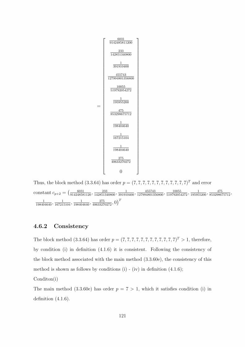
=
60319142485811200
233142851340800
1391910400
455743127994801356800
10055519792054272
1195955200
475853298675712
1198404640
1167215104
1198404640
27540633270272
0
Thus, the block method (3.3.64) has order p = (7, 7, 7, 7, 7, 7, 7, 7, 7, 7, 7, 7)T and error
constant cp+2 =(
6031914248581120
, 233142851340800
, 1391910400
, 455743127994801356800
, 10055519792054272
, 1195955200
, 475853298675712
,
1198404640
, 1167215104
, 1198404640
, 27540633270272
, 0)T
4.6.2 Consistency
The block method (3.3.64) has order p = (7, 7, 7, 7, 7, 7, 7, 7, 7, 7, 7, 7)T > 1, therefore,
by condition (i) in definition (4.1.6) it is consistent. Following the consistency of
the block method associated with the main method (3.3.60e), the consistency of this
method is shown as follows by conditions (i) - (iv) in definition (4.1.6);
Conditon(i)
The main method (3.3.60e) has order p = 7 > 1, which it satisfies condition (i) in
definition (4.1.6).
121

Condition (ii)
The first and second characteristic polynomials of method (3.3.60e) are given respec-
tively by
ρ(z) = z − 2z5/6 + z2/3 (4.5.15)
and
σ(z) = −(−4315z − 53994z5/6 + 2307z2/3 − 7948z1/2 + 4827z1/3 − 1578z1/6 + 221
2177280
)(4.5.16)
From (4.5.15), α2/3 = 1, α5/6 = −2 and α1 = 1 thus∑j
αj = 1− 2 + 1 = 0, j =2
3,
5
6, 1
Condition (iii)
ρ′(r) =1
3r−1/3(3r1/3 − 5r1/6 + 2)
⇒ ρ′(1) = 13(3− 5 + 2) = 0
(4.5.17)
Also by (4.5.15)
ρ(1) = 1− 2 + 1 = 0
... ρ′(1) = ρ(1) = 0
Condition (iv)
From (4.5.17),
ρ′′(z) =1
18r−4/3(5r1/6 − 4)
⇒ ρ′′(1) =1
18(5− 4) =
1
18
Using (4.5.16),
σ(1) =4315 + 53994− 2307 + 7948− 4827 + 1578− 221
2177280=
1
36
2!σ(1) = 2
(1
36
)=
1
18
... ρ′′(1) = 2!σ(1)
122

Thus by definition (4.1.6), the main method (3.3.60e) is consistent.
4.6.3 Zero Stability of the one step Method with Five OffstepPoints
4.5.3.1 Zero stability of the Block Method (3.3.64)
Using (3.3.64) and the definitions in (3.2.12) in the limit as h→ 0 in (4.1.9), the first
characteristic polynomial of the block method is obtained by (4.1.9) as
ρ(z) = det
z
1 0 0 0 0 0 0 0 0 0 0 0
0 1 0 0 0 0 0 0 0 0 0 0
0 0 1 0 0 0 0 0 0 0 0 0
0 0 0 1 0 0 0 0 0 0 0 0
0 0 0 0 1 0 0 0 0 0 0 0
0 0 0 0 0 1 0 0 0 0 0 0
0 0 0 0 0 0 1 0 0 0 0 0
0 0 0 0 0 0 0 1 0 0 0 0
0 0 0 0 0 0 0 0 1 0 0 0
0 0 0 0 0 0 0 0 0 1 0 0
0 0 0 0 0 0 0 0 0 0 1 0
0 0 0 0 0 0 0 0 0 0 0 1
−
0 0 0 0 0 1 0 0 0 0 0 0
0 0 0 0 0 1 0 0 0 0 0 0
0 0 0 0 0 1 0 0 0 0 0 0
0 0 0 0 0 1 0 0 0 0 0 0
0 0 0 0 0 1 0 0 0 0 0 0
0 0 0 0 0 1 0 0 0 0 0 0
0 0 0 0 0 0 0 0 0 0 0 0
0 0 0 0 0 0 0 0 0 0 0 0
0 0 0 0 0 0 0 0 0 0 0 0
0 0 0 0 0 0 0 0 0 0 0 0
0 0 0 0 0 0 0 0 0 0 0 0
0 0 0 0 0 0 0 0 0 0 0 0
123
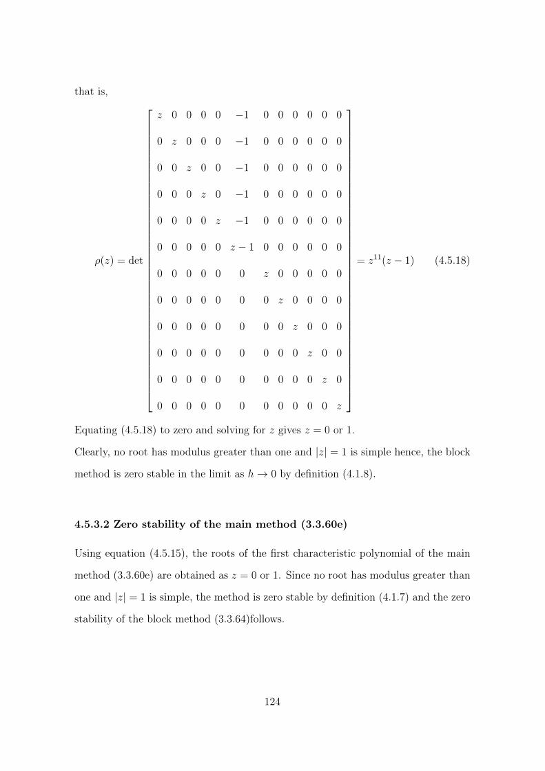
that is,
ρ(z) = det
z 0 0 0 0 −1 0 0 0 0 0 0
0 z 0 0 0 −1 0 0 0 0 0 0
0 0 z 0 0 −1 0 0 0 0 0 0
0 0 0 z 0 −1 0 0 0 0 0 0
0 0 0 0 z −1 0 0 0 0 0 0
0 0 0 0 0 z − 1 0 0 0 0 0 0
0 0 0 0 0 0 z 0 0 0 0 0
0 0 0 0 0 0 0 z 0 0 0 0
0 0 0 0 0 0 0 0 z 0 0 0
0 0 0 0 0 0 0 0 0 z 0 0
0 0 0 0 0 0 0 0 0 0 z 0
0 0 0 0 0 0 0 0 0 0 0 z
= z11(z − 1) (4.5.18)
Equating (4.5.18) to zero and solving for z gives z = 0 or 1.
Clearly, no root has modulus greater than one and |z| = 1 is simple hence, the block
method is zero stable in the limit as h→ 0 by definition (4.1.8).
4.5.3.2 Zero stability of the main method (3.3.60e)
Using equation (4.5.15), the roots of the first characteristic polynomial of the main
method (3.3.60e) are obtained as z = 0 or 1. Since no root has modulus greater than
one and |z| = 1 is simple, the method is zero stable by definition (4.1.7) and the zero
stability of the block method (3.3.64)follows.
124
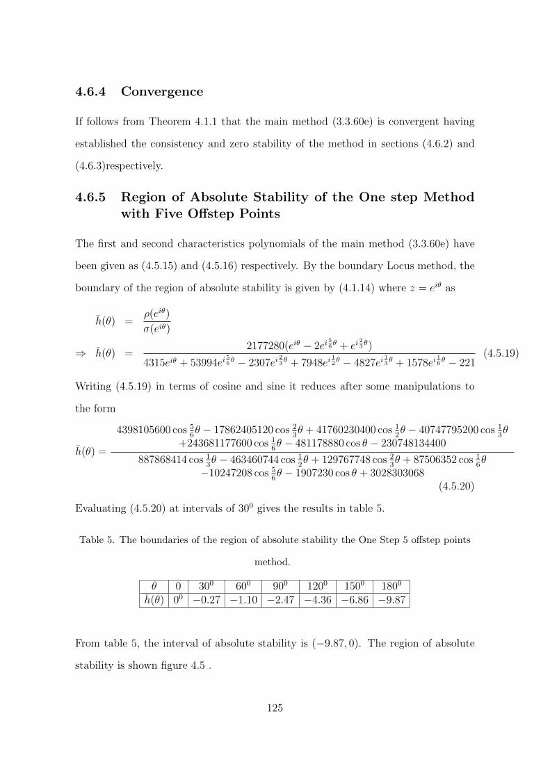
4.6.4 Convergence
If follows from Theorem 4.1.1 that the main method (3.3.60e) is convergent having
established the consistency and zero stability of the method in sections (4.6.2) and
(4.6.3)respectively.
4.6.5 Region of Absolute Stability of the One step Methodwith Five Offstep Points
The first and second characteristics polynomials of the main method (3.3.60e) have
been given as (4.5.15) and (4.5.16) respectively. By the boundary Locus method, the
boundary of the region of absolute stability is given by (4.1.14) where z = eiθ as
h(θ) =ρ(eiθ)
σ(eiθ)
⇒ h(θ) =2177280(eiθ − 2ei
56θ + ei
23θ)
4315eiθ + 53994ei56θ − 2307ei
23θ + 7948ei
12θ − 4827ei
13θ + 1578ei
16θ − 221
(4.5.19)
Writing (4.5.19) in terms of cosine and sine it reduces after some manipulations to
the form
h(θ) =
4398105600 cos 56θ − 17862405120 cos 2
3θ + 41760230400 cos 1
2θ − 40747795200 cos 1
3θ
+243681177600 cos 16θ − 481178880 cos θ − 230748134400
887868414 cos 13θ − 463460744 cos 1
2θ + 129767748 cos 2
3θ + 87506352 cos 1
6θ
−10247208 cos 56θ − 1907230 cos θ + 3028303068
(4.5.20)
Evaluating (4.5.20) at intervals of 300 gives the results in table 5.
Table 5. The boundaries of the region of absolute stability the One Step 5 offstep points
method.
θ 0 300 600 900 1200 1500 1800
h(θ) 00 −0.27 −1.10 −2.47 −4.36 −6.86 −9.87
From table 5, the interval of absolute stability is (−9.87, 0). The region of absolute
stability is shown figure 4.5 .
125
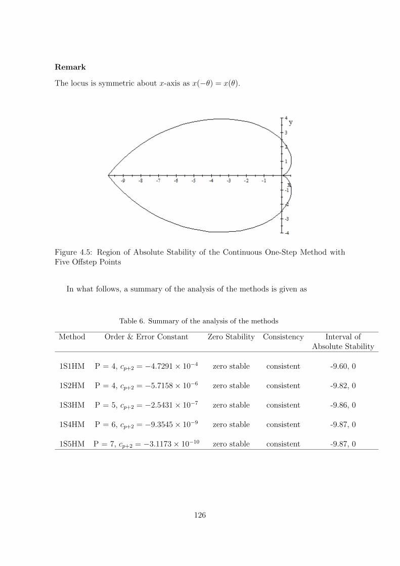
Remark
The locus is symmetric about x-axis as x(−θ) = x(θ).
Figure 4.5: Region of Absolute Stability of the Continuous One-Step Method withFive Offstep Points
In what follows, a summary of the analysis of the methods is given as
Table 6. Summary of the analysis of the methods
Method Order & Error Constant Zero Stability Consistency Interval ofAbsolute Stability
1S1HM P = 4, cp+2 = −4.7291× 10⁻⁴ zero stable consistent -9.60, 0
1S2HM P = 4, cp+2 = −5.7158× 10⁻⁶ zero stable consistent -9.82, 0
1S3HM P = 5, cp+2 = −2.5431× 10⁻⁷ zero stable consistent -9.86, 0
1S4HM P = 6, cp+2 = −9.3545× 10⁻⁹ zero stable consistent -9.87, 0
1S5HM P = 7, cp+2 = −3.1173× 10⁻¹⁰ zero stable consistent -9.87, 0
126
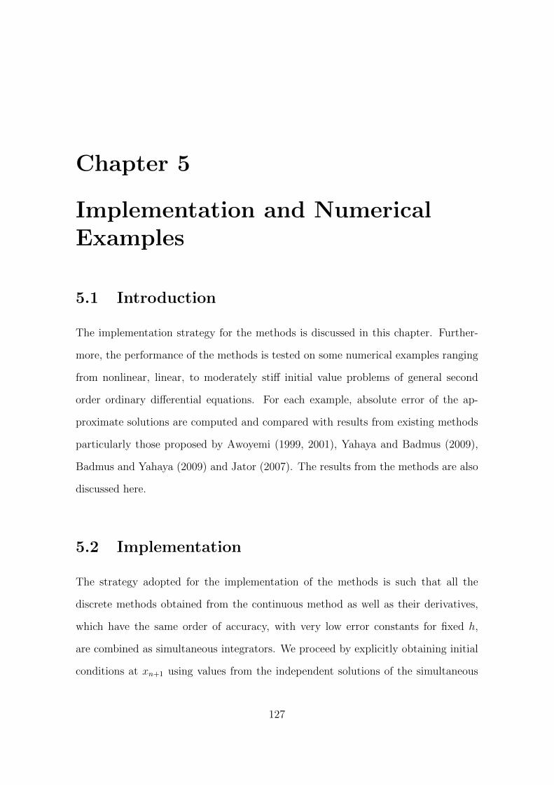
Chapter 5
Implementation and NumericalExamples
5.1 Introduction
The implementation strategy for the methods is discussed in this chapter. Further-
more, the performance of the methods is tested on some numerical examples ranging
from nonlinear, linear, to moderately stiff initial value problems of general second
order ordinary differential equations. For each example, absolute error of the ap-
proximate solutions are computed and compared with results from existing methods
particularly those proposed by Awoyemi (1999, 2001), Yahaya and Badmus (2009),
Badmus and Yahaya (2009) and Jator (2007). The results from the methods are also
discussed here.
5.2 Implementation
The strategy adopted for the implementation of the methods is such that all the
discrete methods obtained from the continuous method as well as their derivatives,
which have the same order of accuracy, with very low error constants for fixed h,
are combined as simultaneous integrators. We proceed by explicitly obtaining initial
conditions at xn+1 using values from the independent solutions of the simultaneous
127

integrators over non-overlapping subintervals; [0, x1], . . . , [xN−1, xN ] (Yusuph & On-
umanyi, 2005); to implement the respective methods proposed. The absolute errors
calculated in the code are defined as
Erc = |yc− yex|
where yex is the exact solution, yc is the computed result and Erc is the absolute
error.
All computations were carried out using FORTRAN codes in FORTRAN 95 lan-
guage and executed on Windows XP operating system. The computer codes are
simply written without the use of subroutines and requires no previous knowledge of
programing before it can be used.
5.3 Numerical Examples
In order to study the efficiency of the developed methods, we present some numer-
ical experiments with the following five problems. The Continuous Implicit Hybrid
One Step Methods (CIHOSM): 1S1HM, 1S2HM, 1S3HM, 1S4HM and 1S5HM, were
applied to solve the following test problems:
1. xy′′ − x+ 3y′ −(
3
x
)y, x0 = 1, y(x0) = 2, y′(x0) = 10
Exact Solution: y = 3x3 − 2x+ x2(1 + x lnx)
h =0.1
32
Source: Awoyemi (1999)
2. y′′ − x(y′)2 = 0, y(0) = 1, y′(0) =1
2
Exact solution: y = 1 +1
2ln
(2 + x
2− x
)h =
0.1
32
Source: Awoyemi (2001)
128

3. y′′ = y′, y(0) = 0, y′(0) = −1
Exact solution: y(x) = 1− exp(x)
h = 0.1
Source: Yahaya & Badmus (2009)
4. y′′ + 1001y′ + 1000y = 0, y(0) = 1, y′(0) = −1
Exact solution: y(x) = exp(−x)
h = 0.05
Source: Jator (2007)
5. y′′ +
(6
x
)y′ +
(4
x2
)y = 0, y(1) = 1, y′(1) = 1
Exact solution:5
3x− 3
3x4
h =0.1
32
Source: Badmus & Yahaya (2009)
The following notations are used in the tablesx Point of Evaluation
Y ex Exact solution
1S1HM one step, One offstep point method
1S2HM one step, Two offstep points method
1S3HM one step, Three offstep points method
1S4HM one step, Four offstep points method
1S5HM one step, Five offstep points method
Erc Absolute error
The computed results for the five problems using the five methods proposed are
presented in tables 7 to 16.
129

Table 7. Showing the exact solutions and the computed results from the proposed methods forProblem 1.
X YEX 1S1HM 1S2HM 1S3HM 1S4HM 1S5HM1.1 0.31298579E+01 0.31298580E+01 0.31298579E+01 0.31298579E+01 0.31298579E+01 0.31298579E+01
1.2 0.45390517E+01 0.45390516E+01 0.45390517E+01 0.45390517E+01 0.45390517E+01 0.45390517E+01
1.3 0.62574144E+01 0.62574142E+01 0.62574143E+01 0.62574143E+01 0.62574144E+01 0.62574144E+01
1.4 0.83152800E+01 0.83152797E+01 0.83152798E+01 0.83152799E+01 0.83152800E+01 0.83152799E+01
1.5 0.10743445E+02 0.10743445E+02 0.10743445E+02 0.10743445E+02 0.10743445E+02 0.10743445E+02
1.6 0.13573135E+02 0.13573135E+02 0.13573135E+02 0.13573135E+02 0.13573135E+02 0.13573135E+02
1.7 0.16835977E+02 0.16835976E+02 0.16835977E+02 0.16835977E+02 0.16835977E+02 0.16835977E+02
1.8 0.20563972E+02 0.20563971E+02 0.20563972E+02 0.20563972E+02 0.20563973E+02 0.20563972E+02
1.9 0.24789476E+02 0.24789475E+02 0.24789476E+02 0.24789476E+02 0.24789477E+02 0.24789476E+02
2.0 0.29545178E+02 0.29545176E+02 0.29545177E+02 0.29545178E+02 0.29545179E+02 0.29545178E+02
Table 8: Comparing the absolute errors in the new methods to errors in Awoyemi(1999) for Problem 1
X Error in 1S1HM Error in 1S2HM Error in 1S3HM Error in 1S4HM Error in 1S5HM Error inp=4, k=1 p=4, k=1 p=5, k=1 p=6, k=1 p=7, k=1 Awoyemi(1999)
p=4, k=2
1.1 0.12888106E-07 0.57475482E-08 0.24871327E-08 0.19055255E-08 0.14318067E-08 0.51125591E-07
1.2 0.54913644E-07 0.24458675E-07 0.10363642E-07 0.80201747E-08 0.60836944E-08 –
1.3 0.13065430E-06 0.58169761E-07 0.24154704E-07 0.18919443E-07 0.14459401E-07 0.52074859E-06
1.4 0.24455343E-06 0.10885790E-06 0.44309187E-07 0.35151302E-07 0.27047847E-07 –
1.5 0.40094191E-06 0.17845020E-06 0.71207941E-07 0.57235781E-07 0.44325446E-07 0.15996662E-05
1.6 0.60406071E-06 0.26883387E-06 0.10517184E-06 0.85669157E-07 0.66758535E-07 –
1.7 0.85807786E-06 0.38186365E-06 0.14646803E-06 0.12092716E-06 0.94805369E-07 0.34250638E-05
1.8 0.11671012E-05 0.51936759E-06 0.19531497E-06 0.16346750E-06 0.12891749E-06 –
1.9 0.15351888E-05 0.68315154E-06 0.25188674E-06 0.21373182E-06 0.16954080E-06 0.61293258E-05
2.0 0.19663562E-05 0.87500259E-06 0.31631626E-06 0.27214757E-06 0.21711659E-06 0.78514782E-05
130

Table 9. Showing the exact solutions and the computed results from the proposed methods forProblem 2
X YEX 1S1HM 1S2HM 1S3HM 1S4HM 1S5HM0.1 0.10500417E+01 0.10500417E+01 0.10500417E+01 0.10500417E+01 0.10500417E+01 0.10500417E+01
0.2 0.11003353E+01 0.11003353E+01 0.11003353E+01 0.11003353E+01 0.11003354E+01 0.11003354E+01
0.3 0.11511404E+01 0.11511404E+01 0.11511404E+01 0.11511404E+01 0.11511404E+01 0.11511404E+01
0.4 0.12027326E+01 0.12027326E+01 0.12027326E+01 0.12027326E+01 0.12027326E+01 0.12027326E+01
0.5 0.12554128E+01 0.12554128E+01 0.12554128E+01 0.12554128E+01 0.12554128E+01 0.12554128E+01
0.6 0.13095196E+01 0.13095196E+01 0.13095196E+01 0.13095196E+01 0.13095196E+01 0.13095196E+01
0.7 0.13654438E+01 0.13654437E+01 0.13654438E+01 0.13654438E+01 0.13654438E+01 0.13654438E+01
0.8 0.14236489E+01 0.14236489E+01 0.14236489E+01 0.14236489E+01 0.14236489E+01 0.14236489E+01
0.9 0.14847003E+01 0.14847002E+01 0.14847003E+01 0.14847003E+01 0.14847003E+01 0.14847003E+01
1.0 0.15493062E+01 0.15493060E+01 0.15493061E+01 0.15493061E+01 0.15493062E+01 0.15493062E+01
Table 10. Comparing the absolute errors in the new methods to errors in Awoyemi(2001) for Problem2.
X Error in 1S1HM Error in 1S2HM Error in 1S3HM Error in 1S4HM Error in 1S5HM Error inp=4, k=1 p=4, k=1 p=5, k=1 p=6, k=1 p=7, k=1 Awoyemi(2001)
p=6, k=4
0.1 0.49827253E-10 0.22413627E-10 0.12381429E-10 0.76769702E-11 0.69253492E-11 0.26075253E-09
0.2 0.41043058E-09 0.18330515E-09 0.10142642E-09 0.62873262E-10 0.56260108E-10 0.19816704E-08
0.3 0.14285815E-08 0.63686190E-09 0.35245495E-09 0.21852276E-09 0.19460211E-09 0.65074122E-08
0.4 0.35242687E-08 0.15698642E-08 0.86895491E-09 0.53898974E-09 0.47769566E-09 0.15592381E-07
0.5 0.72435324E-08 0.32251910E-08 0.17857029E-08 0.11083281E-08 0.97695985E-09 0.31504477E-07
0.6 0.13335597E-07 0.59361429E-08 0.32879226E-08 0.20423685E-08 0.17889177E-08 0.56374577E-07
0.7 0.22872871E-07 0.10179837E-07 0.56411280E-08 0.35075920E-08 0.30497800E-08 0.96164046E-07
0.8 0.37447019E-07 0.16664477E-07 0.92399235E-08 0.57519813E-08 0.49590416E-08 0.15686801E-06
0.9 0.59503708E-07 0.26478362E-07 0.14691385E-07 0.91578443E-08 0.78195337E-08 0.24869769E-06
1.0 0.92940412E-07 0.41356017E-07 0.22964069E-07 0.14336313E-07 0.12108436E-07 0.38798389E-06
131
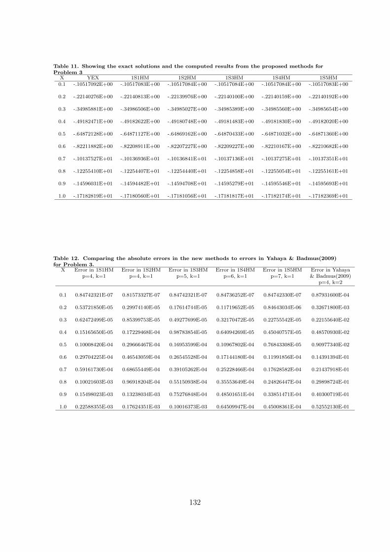
Table 11. Showing the exact solutions and the computed results from the proposed methods forProblem 3
X YEX 1S1HM 1S2HM 1S3HM 1S4HM 1S5HM0.1 -.10517092E+00 -.10517083E+00 -.10517084E+00 -.10517084E+00 -.10517084E+00 -.10517083E+00
0.2 -.22140276E+00 -.22140813E+00 -.22139976E+00 -.22140100E+00 -.22140159E+00 -.22140192E+00
0.3 -.34985881E+00 -.34986506E+00 -.34985027E+00 -.34985389E+00 -.34985560E+00 -.34985654E+00
0.4 -.49182471E+00 -.49182622E+00 -.49180748E+00 -.49181483E+00 -.49181830E+00 -.49182020E+00
0.5 -.64872128E+00 -.64871127E+00 -.64869162E+00 -.64870433E+00 -.64871032E+00 -.64871360E+00
0.6 -.82211882E+00 -.82208911E+00 -.82207227E+00 -.82209227E+00 -.82210167E+00 -.82210682E+00
0.7 -.10137527E+01 -.10136936E+01 -.10136841E+01 -.10137136E+01 -.10137275E+01 -.10137351E+01
0.8 -.12255410E+01 -.12254407E+01 -.12254440E+01 -.12254858E+01 -.12255054E+01 -.12255161E+01
0.9 -.14596031E+01 -.14594482E+01 -.14594708E+01 -.14595279E+01 -.14595546E+01 -.14595693E+01
1.0 -.17182819E+01 -.17180560E+01 -.17181056E+01 -.17181817E+01 -.17182174E+01 -.17182369E+01
Table 12. Comparing the absolute errors in the new methods to errors in Yahaya & Badmus(2009)for Problem 3.
X Error in 1S1HM Error in 1S2HM Error in 1S3HM Error in 1S4HM Error in 1S5HM Error in Yahayap=4, k=1 p=4, k=1 p=5, k=1 p=6, k=1 p=7, k=1 & Badmus(2009)
p=4, k=2
0.1 0.84742321E-07 0.81573327E-07 0.84742321E-07 0.84736252E-07 0.84742330E-07 0.87931600E-04
0.2 0.53721850E-05 0.29974140E-05 0.17614744E-05 0.11719652E-05 0.84643034E-06 0.32671800E-03
0.3 0.62472499E-05 0.85399753E-05 0.49277699E-05 0.32170472E-05 0.22755542E-05 0.22155640E-02
0.4 0.15165650E-05 0.17229468E-04 0.98783854E-05 0.64094269E-05 0.45040757E-05 0.48570930E-02
0.5 0.10008420E-04 0.29666467E-04 0.16953599E-04 0.10967802E-04 0.76843308E-05 0.90977340E-02
0.6 0.29704225E-04 0.46543059E-04 0.26545528E-04 0.17144180E-04 0.11991856E-04 0.14391394E-01
0.7 0.59161730E-04 0.68655449E-04 0.39105262E-04 0.25228466E-04 0.17628582E-04 0.21437918E-01
0.8 0.10021603E-03 0.96918204E-04 0.55150938E-04 0.35553649E-04 0.24826447E-04 0.29898724E-01
0.9 0.15498023E-03 0.13238034E-03 0.75276848E-04 0.48501651E-04 0.33851471E-04 0.40300719E-01
1.0 0.22588355E-03 0.17624351E-03 0.10016373E-03 0.64509947E-04 0.45008361E-04 0.52552130E-01
132
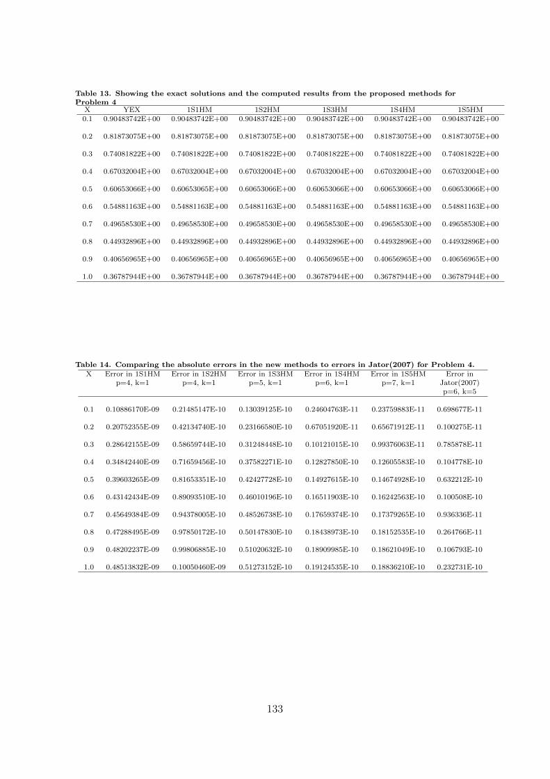
Table 13. Showing the exact solutions and the computed results from the proposed methods forProblem 4
X YEX 1S1HM 1S2HM 1S3HM 1S4HM 1S5HM0.1 0.90483742E+00 0.90483742E+00 0.90483742E+00 0.90483742E+00 0.90483742E+00 0.90483742E+00
0.2 0.81873075E+00 0.81873075E+00 0.81873075E+00 0.81873075E+00 0.81873075E+00 0.81873075E+00
0.3 0.74081822E+00 0.74081822E+00 0.74081822E+00 0.74081822E+00 0.74081822E+00 0.74081822E+00
0.4 0.67032004E+00 0.67032004E+00 0.67032004E+00 0.67032004E+00 0.67032004E+00 0.67032004E+00
0.5 0.60653066E+00 0.60653065E+00 0.60653066E+00 0.60653066E+00 0.60653066E+00 0.60653066E+00
0.6 0.54881163E+00 0.54881163E+00 0.54881163E+00 0.54881163E+00 0.54881163E+00 0.54881163E+00
0.7 0.49658530E+00 0.49658530E+00 0.49658530E+00 0.49658530E+00 0.49658530E+00 0.49658530E+00
0.8 0.44932896E+00 0.44932896E+00 0.44932896E+00 0.44932896E+00 0.44932896E+00 0.44932896E+00
0.9 0.40656965E+00 0.40656965E+00 0.40656965E+00 0.40656965E+00 0.40656965E+00 0.40656965E+00
1.0 0.36787944E+00 0.36787944E+00 0.36787944E+00 0.36787944E+00 0.36787944E+00 0.36787944E+00
Table 14. Comparing the absolute errors in the new methods to errors in Jator(2007) for Problem 4.
X Error in 1S1HM Error in 1S2HM Error in 1S3HM Error in 1S4HM Error in 1S5HM Error inp=4, k=1 p=4, k=1 p=5, k=1 p=6, k=1 p=7, k=1 Jator(2007)
p=6, k=5
0.1 0.10886170E-09 0.21485147E-10 0.13039125E-10 0.24604763E-11 0.23759883E-11 0.698677E-11
0.2 0.20752355E-09 0.42134740E-10 0.23166580E-10 0.67051920E-11 0.65671912E-11 0.100275E-11
0.3 0.28642155E-09 0.58659744E-10 0.31248448E-10 0.10121015E-10 0.99376063E-11 0.785878E-11
0.4 0.34842440E-09 0.71659456E-10 0.37582271E-10 0.12827850E-10 0.12605583E-10 0.104778E-10
0.5 0.39603265E-09 0.81653351E-10 0.42427728E-10 0.14927615E-10 0.14674928E-10 0.632212E-10
0.6 0.43142434E-09 0.89093510E-10 0.46010196E-10 0.16511903E-10 0.16242563E-10 0.100508E-10
0.7 0.45649384E-09 0.94378005E-10 0.48526738E-10 0.17659374E-10 0.17379265E-10 0.936336E-11
0.8 0.47288495E-09 0.97850172E-10 0.50147830E-10 0.18438973E-10 0.18152535E-10 0.264766E-11
0.9 0.48202237E-09 0.99806885E-10 0.51020632E-10 0.18909985E-10 0.18621049E-10 0.106793E-10
1.0 0.48513832E-09 0.10050460E-09 0.51273152E-10 0.19124535E-10 0.18836210E-10 0.232731E-10
133
Table 15. Showing the exact solutions and the computed results from the proposed methods forProblem 5.
X YEX 1S1HM 1S2HM 1S3HM 1S4HM 1S5HM1.0031 0.10030765E+01 0.10030765E+01 0.10030765E+01 0.10030765E+01 0.10030765E+01 0.10030765E+01
1.0063 0.10060575E+01 0.10060575E+01 0.10060575E+01 0.10060575E+01 0.10060575E+01 0.10060575E+01
1.0094 0.10089450E+01 0.10089450E+01 0.10089450E+01 0.10089450E+01 0.10089450E+01 0.10089450E+01
1.0125 0.10117410E+01 0.10117410E+01 0.10117410E+01 0.10117410E+01 0.10117410E+01 0.10117410E+01
1.0156 0.10144475E+01 0.10144476E+01 0.10144476E+01 0.10144475E+01 0.10144475E+01 0.10144475E+01
1.0188 0.10170665E+01 0.10170665E+01 0.10170665E+01 0.10170665E+01 0.10170665E+01 0.10170665E+01
1.0219 0.10195998E+01 0.10195998E+01 0.10195998E+01 0.10195998E+01 0.10195998E+01 0.10195998E+01
1.0250 0.10220492E+01 0.10220492E+01 0.10220492E+01 0.10220492E+01 0.10220492E+01 0.10220492E+01
1.0281 0.10244165E+01 0.10244166E+01 0.10244166E+01 0.10244165E+01 0.10244165E+01 0.10244165E+01
1.0313 0.10267036E+01 0.10267037E+01 0.10267036E+01 0.10267036E+01 0.10267036E+01 0.10267036E+01
Table 16. Comparing the absolute errors in the new methods to errors in Badmus & Yahaya (2009)for Problem 5.
X Error in 1S1HM Error in 1S2HM Error in 1S3HM Error in 1S4HM Error in 1S5HM Error in Badmusp=4, k=1 p=4, k=1 p=5, k=1 p=6, k=1 p=7, k=1 & Yahaya(2009)
p=4, k=2
1.0031 0.81807894E-11 0.77022833E-11 0.77009510E-11 0.77586826E-11 0.76998408E-11 0.38354E-04
1.0063 0.27785485E-08 0.12658126E-08 0.71779915E-09 0.45977178E-09 0.41327297E-09 0.75004E-04
1.0094 0.74754114E-08 0.33850827E-08 0.19176578E-08 0.12299799E-08 0.10432657E-08 0.10592E-03
1.0125 0.13997774E-07 0.63126238E-08 0.35708470E-08 0.22894449E-08 0.18729474E-08 0.13548E-03
1.0156 0.22264084E-07 0.10012317E-07 0.56571030E-08 0.36252337E-08 0.28933289E-08 0.15557E-03
1.0188 0.32195759E-07 0.14449356E-07 0.81569016E-08 0.52248852E-08 0.40957480E-08 0.18637E-03
1.0219 0.43717076E-07 0.19590206E-07 0.11051428E-07 0.70763917E-08 0.54718601E-08 0.19606E-03
1.0250 0.56755078E-07 0.25402552E-07 0.14322554E-07 0.91681831E-08 0.70136241E-08 0.22104E-03
1.0281 0.71239469E-07 0.31855260E-07 0.17952815E-07 0.11489112E-07 0.87132936E-08 0.20563E-03
1.0313 0.87102518E-07 0.38918333E-07 0.21925381E-07 0.14028440E-07 0.99304354E-08 0.27791E-03
134

5.4 Discussion of the Results
Computer programs written for the implementation of the five Continuous Implicit
Hybrid One Step Methods (CIHOSM) developed namely: 1S1HM, 1S2HM, 1S3HM,
1S4HM and 1S5HM; were tested respectively on five numerical examples which are,
respectively, nonlinear, linear and stiff initial value problems of general second order
ordinary differential equations in the last section.
The approximate solutions obtained from these experiments elucidated the effi-
ciency of the computed programs.
It is observed from the tables that the results obtained from the methods con-
verged faster when the number of offstep points were increased. This validates the
consistency and zero stability of the methods and agrees with the fact that, as the
step size h decreases, the methods get more accurate as demonstrated in Table 5.
Even though there are some deviations in what is obtained in Table 12, where the
results obtained at x = 0.3 to 0.7 by 1S1HM are better than those from 1S2HM for
the moderately stiff problem 3.
Generally, the performance of our methods as noticed in tables 7 to 16, are superior
to those from methods implemented on the predictor-corrector codes by Awoyemi
(1999 and 2001) and the block methods proposed by Yahaya and Badmus (2009) and
Badmus and Yahaya (2009) for the same step sizes, even though their method had
higher step numbers.
However, even though the multiple finite difference method of Jator (2007) seemed
to have produced a better result at most of the points of evaluation, it should be
noticed that the method had step number k = 5 against our methods with step
number k = 1. Indeed, our methods compared favourably with Jator (2007) results
given the obvious differences in their designs.
135

It should be noticed that, as the offstep points are decreasing, the step size becomes
smaller and the methods become more accurate for the five problems used to test the
accuracy of the methods just as small steps in the finite elements methods increase
the accuracy of the problems solved.
Also, beyond the reduction in step number which means lesser function evaluations
per iteration, this approach produced higher order discrete methods which give very
low error terms and wider intervals of absolute stability.
136
Chapter 6
Summary and Conclusion
6.1 Introduction
In this chapter, a general conclusion on the research work is made. Recommendations
on the proposed class of methods is made while areas of further research are suggested.
6.2 Summary and Conclusion
A class of hybrid collocation methods for the direct solution of initial value problems
of general second-order ordinary differential equations have been developed in this
research. The collocation technique yielded very consistent and zero stable implicit
hybrid one step methods with continuous coefficients. The methods are implemented
without the need for the development of predictors nor requiring any other method
to generate starting values. Furthermore, the inclusion of offstep points allowed the
adoption of linear multistep procedure, circumvent the ‘zero-stability barrier’, up-
graded the order of accuracy of the methods and to obtain very low error constants.
In particular, the performance of the methods improved as the number of off-
step points increased. Adequate stability intervals are obtained for both non-stiff
and stiff problems. Results from the numerical solutions of non-linear, linear and
moderately stiff IVP show that this class of methods are superior to the predictor-
137

corrector method proposed by Awoyemi (1999, 2001), the multiple finite difference
methods proposed by Jator (2007) and the hybrid block method proposed by Yahaya
and Badmus (2009) and Badmus and Yahaya (2009).
All computations were carried out by computer programs written in FORTRAN
95 language, compiled and executed using PLATO FORTRAN 95 on the Windows
XP operating system. The computer programs do not contain subroutines which
means lesser computing time.
6.3 Open Problems
The class of continuous Implicit one step hybrid methods proposed in this thesis is
recommended for the direct solution of initial value problems of general second order
ordinary differential equations; of the nonlinear, linear and stiff types for small h, as
demonstrated by the results of this research in terms of efficiency and accuracy and
ease of implementation.
However, further research could extend the methods to the direct solution of higher
order general ODEs in view of the advantages of these methods.
The plausibility of using other basis functions in place of the power series polyno-
mial used in this work is also suggested for further research in this direction.
Systems of special and general higher order ODEs can be considered using the
new methods proposed in this work.
6.4 Contribution to Knowledge
This research has led to the following contributions:
(i) a new class of continuous implicit hybrid one step methods for the direct solution
of general second-order IVPs of ODE has been developed;
138

(ii) a new hybrid block formula has been defined; and
(iii) very accurate and highly efficient computer codes have been written for the
implementation of the new methods
139

References
Adee, S.O., Onumanyi, P., Sirisena, U.W. & Yahaya, Y.A. (2005). Note on Starting the
Numerov Method More Accurately by a Hybrid Formula of Order Four for Initial
Value Problems. Journal of Computational and Applied Mathematics, 175, 369-373.
Ademiluyi, R.A. & Kayode, S.J. (2001). Maximum Order Second Derivative Hybrid Mul-
tistep Method for Integration of Initial Value Problems of Ordinary Differential Equa-
tions. Journal of Nigerian Association of Mathematical Physics, 5, 251-262.
Adesanya, A.O., Anake, T.A. & Udoh, M.O. (2008). Improved Continuous Method for
Direct Solution of General Second Order Ordinary Differential Equations. Journal of
Nigerian Association of Mathematical Physics, 13, 59-62.
Adesanya, A.O., Anake, T.A. & Oghoyon, G.J. (2009). Continuous Implicit Method for
the Solution of General Second Order Ordinary Differential Equations. Journal of
Nigerian Association of Mathematical Physics, 15, 71-78.
Awoyemi, D.O.(1992). On some Continuous Linear Multistep Methods for Initial Value
Problems. Unpublished doctoral dissertation, University of Ilorin, Ilorin, Nigeria.
Awoyemi, D.O. (1994a). A Class of Continuous Integration Methods for the First Order
Initial Value Problems in Ordinary Differential Equations. Spectrum Journal, 52-61.
Awoyemi, D.O. (1994b). A 4th-Order Continuous Hybrid Multistep Method for Initial
Value Problems of Second Order Differential Equations. Spectrum Journal, 1 (2),
140

70-73.
Awoyemi, D.O. (1995). A Two Step Hybrid Multistep Method with Continuous Coef-
ficients for Initial Value Problems of General Second Order Differential Equations.
Spectrum Journal, 2 (1 & 2), 56-63.
Awoyemi, D.O. (1998). A Class of Continuous Stormer-Cowell Type Methods for Special
Second Order Ordinary Differential Equations. Spectrum Journal, 5 (1 & 2), 100-108.
Awoyemi, D.O. (1999). A Class of Continuous Methods for General Second Order Initial
Value Problem in Ordinary Differential Equations. International Journal of Com-
puter Mathematics, 72, 29-37.
Awoyemi, D.O. (2001). A New Sixth-Order Algorithm for General Second Order Ordinary
Differential Equations. International Journal of Computer Mathematics, 77, 117-
124.
Awoyemi, D.O. (2003). A P-stable Linear Multistep Method for Solving General Third
Order Ordinary Differential Equations. International Journal of Computer Mathe-
matics, 80 (8), 987-993.
Awoyemi, D.O. (2005). Algorithmic Collocation Approach for Direct Solution of Fourth-
Order Initial-Value Problems of Ordinary Differential Equations. International Jour-
nal of Computer Mathematics, 82 (3), 321-329.
Awoyemi, D.O. & Kayode, S.J. (2005). A Maximal Order Collocation Method for Direct
Solution of Initial Value Problems of General Second Order Ordinary Differential
Equations. In: Proceedings of the Conference Organized by the National Mathemat-
ical Centre, Abuja, Nigeria.
141

Awoyemi, D.O. and Idowu O.M. (2005). A Class of Hybrid Collocation Methods for Third-
Order Ordinary Differential Equations. Internationa Journal of Computer Mathemat-
ics, 82 (10), 1287-1293.
Awoyemi, D.O., Adesanya, A.O. and Ogunyebi, S.N. (2009). Construction of Self-Starting
Numerov Method for the Solutions of Initial Value Problems of General Second Order
Ordinary Differential Equations. Journ. Num. Math., 4 (2), 267-278.
Badmus, A.M. and Yahaya, Y.A. (2009). An Accurate Uniform Order 6 Block Method
for Direct Solution of General Second Order Ordinary Differential Equations. Pacific
Journal of Science and Technology, 10 (2), 248-254.
Brugnano, L. & Trigiante, D. (1998). Solving Differential Problems by Multistep Initial
and Boundary Value Methods. Amsterdam: Gordon and Breach Science Publishers.
Brush, D.G., Kohfield, J.J. & Thompson G.T. (1967). Solution of Ordinary Dif-
ferential Equations Using Two “Off-step” points. Journal of the ACM, 14 (4),
769-784.
Bun, R.A. & Vasil’Yev, Y.D. (1992). A Numerical Method for Solving Differential
Equations of any Orders. Comp. Math. Phys., 32 (3), 317-330.
Butcher, J. (1964). Implicit Runge-Kutta Processes. Math. Comp., 18, 50-64. (MR
28 # 2641).
Butcher, J.C. (1965).A modified Multistep Method for the Numerical Integration of
Ordinary Differential Equations. Journal of the ACM, 12, 124-135.
Butcher, J.C. (2003). Numerical Methods for Ordinary Differential Equations. West
Sussex: John Wiley & Sons Ltd.
142

Cash, J.R. (1981). High Order P-stable Formulae for the Numerical Integration of
Periodic Initial Value Problems. Numerische Mathematik, 37, 355-370.
Ceschino, F. & Kuntzmann, J. (1963). Numerical Solution of Initial Value Problems.
Englewood Cliffs, New Jersey: Prentice-Hall.
Chawla, M.M. (1981). Two-step Fourth Order P -stable Methods for Second Order
Differential Equations. BIT, 21, 190-193.
Chawla, M.M. & McKee, S. (1986). Convergence of Linear Multistep Methods with
Multiple Roots. Journal of Computational and Applied Mathematics, 14, 451-
454.
Chawla, M.M. & Neta, B. (1986). Families of Two-step Fourth Order P-stable
Methods for Second Order Differential Equations. Journal of Computational
and Applied Mathematics, 14, 447-450.
Chawla, M.M. & Rao, P.S. (1985). High Accuracy P-stable Methods for y′′ = f(x, y).
IMA Journal of Numerical Analysis, 5, 215-220.
Chawla, M.M. & Sharma, S.R. (1981). Families of Fifth Order Nystrom Methods
for y′′ = f(x, y) and Intervals of Periodicity. Computing, 26, 247-256.
Chawla, M.M. & Sharma, S.R. (1985). Families of Three-Stage Third Order Runge-
Kutta-Nystrom Methods for y′′ = f(x, y, y′). Journal of the Australian Mathe-
matical Society, 26, 375-386.
Chawla, M.M. & Subramanian, R. (1984). Regions of Absolute Stability of Explicit
Runge-Kutta-Nystrom Methods for y′′ = f(x, y, y′). Journal of Computational
and Applied Mathematics, 11, 259-266.
143
Chollom, J.P., Ndam, J.N. & Kumleng, G.M. (2007). On Some Properties of the
Block Linear Multistep Methods. Science World Journal, 2 (3), 11-17.
Chu, M.T. & Hamilton, H. (1987). Parallel Solution of Ordinary Differential Equa-
tions by Multiblock Methods. SIAM Journal of Scientific and Statistical Com-
putations, 8, 342-553.
Conte, S.D. & de Boor, Carl (1980). Elementary Numerical Analysis: An Algorith-
mic Approach. New York : McGraw-Hill Book Company.
Dahlquist, G. (1956). Convergence and Stability in the Numerical Integration of
ODEs. New York: Academic Press.
Dahlquist, G. (1959). Stability and Error Bounds in the Numerical Integration of
ODEs. Transcript, 130, Royal Institute of Technology, Stockholm.
Dahlquist, G. (1963). A Special Stability Problem for Linear Multistep Methods.
BIT, 3, 27-43.
Dahlquist, G. (1978). On Accuracy and Unconditional Stability of LMM for Second
Order Differential Equations. BIT, 18, 133-136.
D’Ambrosio, R., Ferro, M. and Paternoster, B. (2009). Two-Step Hybrid Collocation
Methods for y′′ = f(x, y). Applied Mathematics Letters, 22, 1076-1080.
Dodes, I.A. (1978). Numerical Analysis for Computer Science. North Holland, New
York: Oxford.
Dormand, J.R. & Prince, P.J., (1987). Runge-Kutta-Nystrom triples. Computers
and Mathematics with Applications, 13, 937-949.
144

Enright, W.H. (1974). Second Derivative Multistep Methods for Stiff ODEs. SIAM
Journal of Numerical Analysis, 11, 321-331.
Enright, W.H. & Addison, C.A. (1984). Properties of Multistep Formula Intended
for a Class of Second Order ODEs. SIAM Journal of Numerical Analysis, 20,
327-339.
Fatunla, S.O. (1984). One leg Multistep Method for Second Order Differential Equa-
tions. Computer and Mathematics with Applications, 10, 1-4.
Fatunla, S.O. (1985). One-leg Hybrid Formula for Second Order IVPs. Computers
and Mathematics with Applications, 10, 329-333.
Fatunla, S.O. (1987). Hybrid Formulas with Non-vanishing Interval of Periodicity.
International Journal of Computer Mathematics, 21, 145-159.
Fatunla, S.O. (1988). Numerical Methods for Initial Values Problems in Ordinary
Differential Equations. New York: Academic Press.
Fatunla, S.O. (1991). Block Methods for Second Order IVPs. International Journal
of Computer Mathematics, 42 (9), 55-63.
Fatunla, S.O. (1994). Block Methods for Second Order Initial Value Problems.
International Journal of Computer Mathematics, 41, 55-63.
Gear, C.W. (1964). Hybrid Methods for Initial Value Problems in Ordinary Differ-
ential Equations. SIAM Journal of Numerical Analysis, 2, 69-86.
Gear, C.W. (1971). Numerical Initial Value Problems in Ordinary Differential Equa-
tions. Englewood Cliffs, New Jersey: Prentice-Hall.
145

Gonzalez, J.L. & Thompson, D. (1997). Gettng started with Numerov’s Method.
Comput. Phys., 11 (5); 514-515.
Goult, R.J., Hoskins, R.F. & Pratt, M.J. (1973). Applicable Mathematics for Engi-
neers and Scientists. London: The Macmillan Press Ltd.
Grabbe, E., Ramo, S. & Woolridge, D. (1958). Handbook of Automation, Computa-
tion and Control. Vol. 1: Control Fundamentals, Chap. 14, 14-60, New York:
Wiley.
Gragg, W.B. & Stetter H.J. (1964). Generalized Multistep Predictor-Corrector
Methods. Journal of the ACM, 11, 188-209.
Hairer, E. (1979). Unconditionally Stable Methods for Second Order Differential
Equations. Numerische Mathematik, 32, 373-379.
Hairer, E. & Wanner, G. (1976). A Theory for Nystrom Methods. Numerische
Mathematik, 25, 383-400.
Henrici, P. (1962). Discrete Variable Methods in ODE. New York: John Wiley &
Sons.
Hoffman, J.O. (2001). Numerical Methods for Engineers and Scientists(2nd Ed.).
New York: Marcel Dekker Inc.
Ibrahim, Z.B., Othman, K.I. & Suleiman, M. (2007). Variable Step Block Backward
Differentiation Formula for Solving First Order Stiff ODEs. Proceedings of the
World Congress on Engineering II, July 2-4, 2007, London.
Ibrahim, Z.B., Suleiman, M. & Othman, K.I. (2009). Direct Block Backward Differ-
entiation Formulas for Solving Second Order Ordinary Differential Equations.
146
World Academy of Science, Engineering and Technology 1: Mathematical and
Computational Sciences, 3 (3), 120-122.
Ismail, F., Ken, Y.L. & Othman, M. (2009). Explicit and Implicit 3-point Block
Methods for Solving Special Second Order Ordinary Differential Equations Di-
rectly. International Journal of Math. Analysis, 3 (5), 239-254.
Ixaru, G.L. (1984). Numerical Methods for Differential Equation and Application.
Bucuresti, Romania: Editura Academiei.
Jacques, I. & Judd, C.J. (1987). Numerical Analysis. New York: Chapman & Hall.
Jain, R.K., Kambo, N.S. & Rakesh, G. (1984). A Sixth Order P-stable Symmetric
Multistep Method for Periodic Initial Value Problems of Second Order Differ-
ential Equations. IMA Journal of Numerical Analysis, 4, 117-125.
Jator, S.N. (2001). Improvements in Adams-Moulton Methods for the First Order
Initial Value Problems. Journal of the Tennessee Academy of Science, 76 (2),
57-60.
Jator, S.N. (2007). A Sixth Order Linear Multistep Method for the Direct Solution
of y′′ = f(x, y, y′). International Journal of Pure and Applied Mathematics,
40 (4), 457-472.
Jator, S.N. & Li, J. (2009). A Self-Starting Linear Multistep Method for a Di-
rect Solution of the General Second-Order Initial Value Problem. International
Journal of Computer Mathematics, 86 (5), 827-836.
Jeltsch, R. (1976). A Note on A-stability of Multistep Multiderivative Method. BIT,
16, 74-78.
147

Juan, A. (2001). Numerical Methods for Partial Differential Equations.[Electronic
version]. Retrieved September 22, 2010 from http://pde.fusion.kth.sc
Kadalbajoo, M.K. & Raman, K.S. (1986). Cubic Spline Solution of Boundary Value
Problems Over Infinite Intervals. Journal of Computational and Applied Math-
ematics, 15, 283-291.
Kayode, S.J. (2004). A Class of Maximal Order Linear Multistep Collocation Meth-
ods for Direct Solution of Ordinary Differential Equations. Unpublished doc-
toral dissertation, Federal University of Technology, Akure, Nigeria.
Kayode S.J. (2005). An Improved Numerov Method for Direct Solution of General
Second Order Initial Value Problems of Ordinary Differential Equations. In:
Proceedings of the Seminar Organised by the National Mathematical Centre,
Abuja, Nigeria.
Kayode, S.J. (2009). An efficient zero stable method for Fourth Order Differential
Equations. Int. J. Math. Sci, 1-10.
Kohfield, J.J. (1967). Multistep Methods with Modified Predictors and Correctors.
Journal of the ACM, 14 (1), 155-166.
Kreyzig, Erwin (2006). Advanced Enginering Mathematics (9th Ed.). New Jersey:
John Wiley & Sons, Inc.
Lambert, J.D. (1973). Computational Methods in ODEs. New York: John Wiley.
Lambert, J.D. (1991). Numerical Methods for Ordinary Differential Systems. New
York: John Wiley.
148

Lambert, J.D. & Watson, I.A. (1976). Symmetric Multistep Methods for Periodic
Initial Value Problems. Journ. of Institute of Mathematics and Its Applications,
18, 189-202.
Lie, I. & Norsett, S.P. (1989). Superconvergence for Multistep Collocation. Math.
Comp., 52, 65-79.
Majid, Z.A., Azimi, N.A. & Suleiman, M. (2009). Solving Second Order Ordi-
nary Differential Equations Using Two Point Four Step Direct Implicit Block
Method. European Journal of Scientific Research, 31 (1), 29-36.
Majid, Z.A. & Suleiman, M.B. (2007). Two Point Block Direct Integration Implicit
Variable Step Method for Solving Higher Order Systems of Ordinary Differential
Equations.In: Proceedings of the World Congress on Engineering II, 812-815
Majid, Z.A., Suleiman, M.B. & Omar, Z. (2006). 3-Point Implicit Block Method for
Solving Ordinary Differential Equations. Bulletin of the Malaysian Mathemat-
ical Sciences Society (2), 29 (1), 23-31.
Milne, W.E., (1953). Numerical Solution of Differential Equations. New York:
Wiley.
Morrison, D. & Stoller, L. (1958). A Method for the Numerical Integration of
Ordinary Differential Equations. Math. Comp., 12, 269-272.
Omar, Z.B. & Suleiman, M.B. (1999). Solving Second Order ODEs Directly Us-
ing Parallel 2-point Explicit Block Method. Prosiding Kolokium Kebangsaan
Pengintegrasian Teknologi Dalam Sains Matematik, Universiti Sains Malaysia,
390-395
149
Omar, Z & Suleiman, M. (2003). Parallel R-Point implicit block method for solving
higher order ordinary differential equation directly. Journal of ICT., 3 (1), 53-
66.
Omar, Z.B. & Suleiman, M.B. (2005). Solving Higher Order ODEs Directly Using
Parallel 2-point Explicit Block Method. Matematika, 21 (1), 15-23.
Omar,Z., Suleiman, M.B., Saman, M.Y. & Evans, D.J. (2002). Parallel r-point
explicit block method for solving second order Ordinary Differential Equations
directly. International Journal of Computer and Mathematics, 79 (3), 289-298.
Onumanyi, P. Sinsena, U.W. & Dauda, Y. (2001). Toward Uniformly Accurate
Continuous Finite Difference Approximation of Ordinary Differential Equations.
Bagale Journal of Pure and Applied Science, 1, 5-8.
Onumanyi, P., Awoyemi, D.O., Jator, S.N. & Sirisena, U.W. (1994). New Linear
Multistep Methods with Continuous Coefficients for First Order IVPs. Journal
of the Nigerian Mathematical Society, 13, 37-51.
Onumanyi, P., Oladele, J.O., Adeniyi, R.B. & Awoyemi, D.O. (1993). Derivation
of Finite Difference Methods by Collocation. Abacus; Journal of Mathematical
Association of Nigeria, 83 (2), 72-83.
Onumanyi, P., Sirisena, W.U. & Jator, S.N. (1999). Continuous finite difference ap-
proximations for solving differential equations. International Journal of Com-
puter and Mathematics, 72, 15-27.
Onumanyi, P., Sirisena, W.U. & Chollom, J.P. (2001). Continuous Hybrid Methods
through Multistep Collocation. Abacus; Journal of Mathematical Association
of Nigeria, 58-64.
150

Rosser, J.B. (1967). A Runge-Kutta for all seasons. SIAM Review, 9, 417-452.
Rutishauser, H. (1960). BemerKungen zur Numerischen Integration Gewohlicher
Differential-gleichungen n-ter Ordnung Numerische. Numerische Mathematik,
2, 263-279.
Sarafyan, D. (1965). Multistep Methods for the Numerical Solution of ODEs Made
Self-starting. Technical Report No.495, Mathematics Research Center, Madi-
son, Wisconsin.
Sarafyan, D. (1990). New Algorithms for the Continuous Approximate Solution of
Ordinary Differential Equations and the Upgrading of the Order of the Pro-
cesses. Computer Math. Appl., 20 (1), 77-100.
Shampine, L.F. & Watts, H.A. (1969). Block Implicit one step Methods. Mathe-
matics of Computation, 23 (108), 731-740.
Simos, T.E. (2002). Dissipative Trigonometrically-fitted Methods for Second Order
IVPs with Oscillating Solutions. Int. J. Mod. Phys, 13 (10), 1333-1345.
Sirisena, U.W., Onumanyi, P. & Awoyemi, D.O. (1996). A New Family of Predictor-
Corrector Methods. Spectrum Journal, 140-147.
Stetter, H.J. (1973). Analysis of Discretization Methods for ODEs. Berlin: Springer-
Verlag.
Taiwo, O.A. & Onumanyi, P. (1991). A Collocation Approximation of Singularly
Perturbed Second Order Differential Equations. Computer Mathematics, 39,
205-211.
151

Twizel, E.H. & Khaliq, A.Q.M. (1984). Mutiderivative Methods for Periodic IVPs.
SIAM Journal of Numericla Analysis, 21, 111-121.
Vigo-Aguilar, J. & Ramos, H. (2006). Variable Stepsize Implementation of Multistep
Methods for y′′ = f(x, y, y′). Journal of Computational & Applied Mathematics,
192, 114-131.
Vigo-Aguilar, J. & Ramos, H. (2003). Dissipative Chebyshev exponential-fitted
Methods for Numerical Solution of Second-Order Differential Equations. Jour-
nal Computational & Applied Mathematics, 158, 187-217.
Wend, D.V.V. (1967). Uniqueness of Solutions of Ordinary Differential Equations.
American Mathematical Monthly, 74, 948-950.
Wend, D.V.V. (1969). Existence & Uniqueness of Solutions of Ordinary Differential
Equations. In: Proceedings of the American Mathematical Society, 23 (1), 27-
33.
Yahaya, Y.A. (2007). A note on the construction of Numerous Method through
quadratic continuous Polynomial for the General Second order Ordinary differ-
ential equations. Journal of Nigerian Association of Mathematical Physics, 11,
261-268.
Yahaya, Y.A. & Badmus, A.M. (2009). A Class of Collocation Methods for General
Second Order Ordinary Differential Equations. African Journal of Mathematics
& Computer Science Research, 2 (04), 069-072.
Yusuph, Y. & Onumanyi, P. (2005). New Multiple FDMs through Multistep Col-
location for y′′ = f(x, y). In: Proceedings of the Conference Organized by the
National Mathematical Center, Abuja, Nigeria.
152

Appendices
153


![[Almighty God] Only he who does God's will can enter into the kingdom of heaven](https://static.fdocuments.in/doc/165x107/55d22904bb61ebab1e8b4613/almighty-god-only-he-who-does-gods-will-can-enter-into-the-kingdom.jpg)
![91 [Almighty God] Almighty God's Utterance "All Those Who Do Not Know God Are the Ones Who Resist God"](https://static.fdocuments.in/doc/165x107/55d3a9bcbb61eb203e8b45a7/91-almighty-god-almighty-gods-utterance-all-those-who-do-not-know.jpg)


![[David o. Oyedepo] Anointing for Exploites](https://static.fdocuments.in/doc/165x107/577cb2b21a28aba7118c26cc/david-o-oyedepo-anointing-for-exploites.jpg)

