Continuous drifting games

Yoav FreundAT&T Labs � Research

Shannon Laboratory180 Park Avenue, Room A205Florham Park, NJ 07932, USA

Manfred OpperDepartment of Applied Sciences and Engineering

Aston UniversityB4 7ET Birmingham UK

September 26, 2001

Abstract

We combine the results of [13] and [8] and derive a continuous variantof a large class of drifting games. Our analysis furthers the understanding ofthe relationship between boosting, drifting games and Brownian motion andyields a differential equation that describes the core of the problem.

1 Introduction

In [7], Freund shows that boosting is closely related to a two party game calledthe “majority vote game”. In the last year this work was extended in two ways.

First, in [13] Schapire generalizes the majority vote game to a much moregeneral set of games, called “drifting games”. He gives a recursive formula forsolving these games and derives several generalizations of the boost-by-majorityalgorithm. Solving the game in this case requires numerical calculation of therecursive formula.

1

Second, in [8], Freund derives an adaptive version of the boost-by-majorityalgorithm. To do that he considers the limit of the majority vote game when thenumber of boosting rounds is increased to infinity while the advantage of each voteover random guessing decreases to zero. Freund derives the differential equationsthat correspond to this limit and shows that they are closely related to the equationsthat describe the time evolution of the density of particles undergoing Brownianmotion with drift.

In this paper we combine the results of [13] and [8] and show, for a large setof drifting games, that the limit of small steps exists and corresponds to a typeof Brownian motion. This limit yields a non-linear differential equation whosesolution gives the min-max strategy for the two sides of the game.

We derive the analytical solution of the differential equations for several one-dimensional problems, one of which was previously solved numerically by Schapirein [13].

Our results show that there is a deep mathematical connection between Brow-nian motion, boosting and drifting games. This connection is interesting in andof itself and might have applications elsewhere. Also, by using this connectionwe might be able to derive adaptive boosting algorithms for other problems ofinterest, such as classification into more than two classes and regression.

The paper is organized as follows. In Section 2 we give a short review ofdrifting games and the use of potential functions in their analysis. In the samesection we motivate the study of continuous drifting games. In Section 3 werestrict our attention to drifting games in which the set of allowed steps is finiteand obeys conditions that we call “normality” and “regularity”. We show thatthe recursive equation for normal drifting games, when the drift parameter

�is

sufficiently small, have a particularly simple form. In Section 5 we show why itmakes sense to scale the different parameters of the drifting game in a particularway when taking the small-step limit. In Section 6 we take this limit and derivethe differential equations that govern the game in this limit. In Section 7 we give aphysical interpretation of these differential equations and the game. We concludewith some explicit solutions in Section 8.

2

2 Background

2.1 The drifting game

This game was first described by Schapire in [13], here we present the game us-ing slightly altered notation and terminology. This notation fits better with theextension of the game to the continuous domain developed in this paper.

The drifting game is a game between two opponents: “shepherd” and an “ad-versary”. The shepherd is trying to get � sheep into a desired area, but has onlylimited control over them. The adversary’s goal is to keep as many of the sheepas possible outside the desired area. The game consists of � rounds, indicated by���������� � .

The definition of a drifting game consists of the following things:�� an inner-product vector space over which the norm ������� is defined.��� a subset of which defines the steps the sheep can take.������ �� � a loss function that associates a loss with each location.� �����

is a real valued parameter which indicates the average drift requiredof the adversary. Larger values of

�indicate a stronger constraint on the

adversary. In this paper we study the game for very small values of�.

The game proceeds as follows. Initially, all the sheep are in the origin, whichis indicated by !" �$# for all % �&�'����(� � . Round � consists of the followingsteps:

1. The shepherd chooses weight vectors )+*" for each sheep % �,�����(� � .

2. The adversary chooses a step vector for each sheep -�*"/. � : such that01"3254 ) *" �6- *"87

�01"9254

::: ) *" ::: � (1)

3. The sheep move: *<; 4" � (*">= -�*" .After the game ends, and the position of the sheep are �? ; 4" , the shepherd

suffers the final average loss:

� � ��

01"9254 �A@ B? ;

4" C.

3

2.2 Why are drifting games interesting?

Drifting games were introduced by Schapire in [13] as an abstraction which gen-eralizes the boost-by-majority algorithm [7] and the binomial weights learningalgorithm [5]. In this subsection we describe these relations and provide the mo-tivation for studying drifting games. In the next subsection we motivate the studyof continuous drifting games.

The boost-by-majority algorithm corresponds to a very simple drifting game,the adversary controls the weak learning algorithm, and the shepherd correspondsto the boosting algorithm, the other elements of the game are defined as follows

�� is the real line and the norm �6��� � is the absolute value.��� is the set

��� ��� = ��� .������ �� � is defined to be

�for �� �

and � otherwise.� � ���

corresponds to the requirement that the error of the generated weakhypotheses be at most @ � � � C�� .

In this game each sheep corresponds to a training example. The location of thesheep on the real line corresponds to the number of hypotheses whose predictionon the example is correct. Each hypothesis corresponds to moving those exampleson which the hypothesis is correct one step down and the rest of the examplesone step up. The loss function � associates a loss of 1 with those examples onwhich the majority vote over the weak hypotheses is incorrect. In this game thevectors chosen by the shepherd correspond to the weights the boosting algorithmplaces on the different examples. For complete details of this correspondence seeFreund [7].

Interestingly, this very same game, with a different interpretation for sheepand locations, corresponds to the problem of online learning with expert adviceas well as to an interesting variant of the twenty-one questions game. The onlinelearning problem was studied by Cesa-Binachi et. al in [5]. In this case the sheepcorrespond to the experts and the location of the sheep corresponds to the numberof mistakes made by the experts. An assumption is made that there is an expertwhich makes no more than � mistakes, the identity of this expert is unknown.The goal is to design an algorithm for combining the advice of the experts whichis guaranteed to make the least number of mistakes under the stated assumption.The analysis of this game yields the binomial weights algorithm.

4

The exact same game was described by Spencer in [16] who called it the “bal-ancing vector” game or the “pusher-chooser” game. Aslam and Dhagat refer tothe same game as a “chip” game and used it to analyze a variety of problems(see [2, 6, 3, 1]).

One application of this game which is closely related to the online learningproblem is the twenty questions game, also called “Ulam’s game”, with a fixednumber of lies. This game was studied by Dhagat et al. [6] and by Spencer [17].In the twenty questions game one party holds a secret represented by an integernumber in some range �������� . The second party tries to identify the secret num-ber by asking questions of the form: “Is the number in the set X?”. Clearly, theoptimal strategy for this game is to perform a binary search. The game becomesmuch more interesting if the party holding the secret is allowed to lie up to � times.Where � is an a-priori fixed parameter of the game. The analysis of this game byDhagat et. al. and by Spencer is based on the same drifting game (here called achip game) as both of the previous problems. In this case each sheep correspondsto a possible secret value and the location of the sheep corresponds to the numberof lies that have been made assuming this was the chosen secret. The solutiongiven to this game is essentially identical to the binomial weights algorithm.

Generalizing the drifting game from this simple one-dimensional case pro-vides a general method for designing algorithms for a large class of problems.Among them boosting algorithms for learning problems in which there are morethan two possible labels.

Consider first the case where the number of possible labels is � � . In [13]Schapire describes a reduction of this problem to a drifting game on a ����� 4 . Thisreduction suggests a boosting algorithm for the non-binary learning setup, how-ever, a closed form solution to this game is not known and the calculation of thesolution is computationally expensive (on the other hand, it can be done prior toreceiving the training data). At the end of this paper we show how the techniqueswe develop here can be used to calculate the optimal strategy for this drifting gamefor the case � ��� .

Next, consider designing a boosting algorithm for learning problems in whichthe label is a real valued number. An insightful way of looking at this problemis to think of boosting as a variational optimization method as was suggested byMason et al. [11, 12]. In this view boosting is seen as a gradient descent method infunction space. Each boosting iteration corresponds to adding a simple function tothe existing solution with the goal of minimizing the average loss over the trainingexamples. Mason et al. choose to use the same loss function as the guide for all

5

the boosting iterations. Intuitively, this choice is not optimal because the effect ofa local improvement in the approximation in the first boosting iteration is signifi-cantly smaller than the effect of a similar improvements at the last iteration. Thisis because early improvements are in danger of being corrupted by subsequentiterations while improvements done on the last iteration are guaranteed to stay asthey are. The drifting game is a natural model for this effect. By using the driftinggame analysis we can design boosting algorithms for arbitrary loss functions. Themeaning of “weak hypotheses” in this case are hypotheses whose value is has aslight negative correlation with the error of the approximation function. In the lastsection of this paper we show how to calculate the optimal time-dependent lossfunction for the target losses @�� � ��� C�� and ��� @ ��� @�� � ��� C�� C .

2.3 Why is the continuous limit interesting?

In this paper we consider limits of drifting games in which the size of the stepsdecreases to zero, the number of steps increases to infinity and

�decreases to

zero. The exact form of the limit will be justified in Section 5. In this section wemotivate exploration of this limit.

Our main interest in this limit stems from the fact that it gives us a generalway of designing boosting algorithms that are adaptive. The Adaboost algo-rithm [9, 14] was the first adaptive boosting algorithm and this adaptivity is oneof the main reasons that Adaboost had a much more significant impact on practi-cal machine learning than its two predecessors. We say that Adaboost is adaptivebecause there is no need to make an a-priori assumption on the maximal errorof the weak hypotheses that will be generated during boosting. Instead, the al-gorithm adapts to the accuracy of the hypothesis that it received from the weaklearner, stronger hypotheses cause larger changes in the weights assigned to theexamples and weaker hypotheses cause smaller changes. In [8] Freund presentedthe Brownboost algorithm which is an adaptive variant of the boost by majorityalgorithm. The transition from boost-by-majority to BrownBoost is done by tak-ing the continuous time limit. Freund also shows that in that paper that Adaboostis a special case of the resulting boosting algorithm.

In this paper we combine Freund’s Brownboost algorithm with Schapire’sdrifting games [13] and in this way show how to make any boosting algorithm(which can be represented as a drifting game) adaptive.

Another benefit of taking the continuous limit is simple and elegant mathe-matical structure of the resulting game. While Schapire’s solution of the drifting

6

games is very general, its calculation requires the solution of a complex recursioninvolving minima and maxima. On the other hand, as we shall show in section 4,when

�is sufficiently small, the recursion becomes simpler and does not involve

minima and maxima. Taking the limit of this simplified recursion yields a stochas-tic differential equation that characterizes the optimal potential function for thegame.

The stochastic differential equation is identical to the equations that charac-terize Brownian motion. These equations have been studied extensively both inphysics, in statistical mechanics, and in mathematical economics, in the study ofoption pricing and the Black-Scholes Equation.

4Using this existing work, we can

use techniques that have been developed for solving stochastic differential equa-tions to calculate the optimal strategies for drifting games. In some cases we cando find closed form analytical representation of the optimal potential function. Inother cases, when finding a closed form solution is too hard, it is often possible touse existing numerical algorithms for solving partial differential equations to finda numerical solution. � In Section 8 we provide analytical and numerical solutionsto some simple drifting games.

Finally, the connection established here between Brownian motion and drift-ing games might provide new insights into the workings of systems in which aweak global force field acts on a large number of small elements. Such systemsseem to be quite common in physics and in economics.

2.4 Analysis of drifting games using a potential function

In [13] Schapire shows that drifting games can be solved by defining a potentialfunction � * @ C . Setting the boundary condition � ? @ C � �A@ C and solving therecursion: � * � 4 @ C � � � � ������

� � * @ =�C = ) � � � � ) � ��� (2)

The minimizing vector ) defined the weight vectors that are the min/max strategyfor the shepherd.

One can show (Theorem 1 in [13]) that the average potential is non increasing For a wonderful review of the mathematical underpinning of the Black Scholes equation and

a new game-theoretic analysis of option pricing, see the recent book by Shafer and Vovk [15].�Most of these algorithms use finite element methods that are very similar to the simplified

recursions described above. However, the advantage of using an existing debugged and optimizedsoftware package rather than writing one by yourself should not be overlooked!

7

1" � * @ *<;

4" C � 1" � * � 4 @ *"�C

Hence, one gets the bound on the average loss��

01"3254 � @ ? ;

4" C � � ! @ � # C (3)

3 Normal and regular lattices

We assume that the sheep positions *" are vectors in � � . We restrict the set ofallowed steps � to be a finite set of size

� = � ! ���� � � which spans the space� � and such that � �"92 ! " � �. If a set � satisfies these conditions, we say it is

normal.If the set � is normal and, in addition, satisfies the following two symmetries

for some positive constants � and � , we say it is regular.

1. For any % . � ����(� � , " � " � �2. For any % ��� . � ���� � � such that %��� , " � �� � � �For example, a regular set in � � is

4 � @ � ��� C � � �� @� � � � � C � �� �

� @� � � � � C (4)

Given an inner-product vector space whose dimension is at least�

it is easy toconstruct a regular set � of size

� = � for this space. For any orthonormal set ofsize

�, � 4 ����(� � � we can derive a regular set by setting ! ���(� � to be

! �� � �

�1� 254 � ���� % �������� � � " ��� � = �� � " � � = � � �� ��� �

�1� 254 � �

8

4 The drifting game for small values of �Given that the set � is normal, we can show that, for sufficiently small values of

�, the solution of the game has a particularly simple form.

Theorem 1 Let � be a normal set of steps. Then there exists some�

!�,�

suchthat for any potential function � * and location and any

�

! 7� 7 �

the solutionto the recursive definition of � * � 4 satisfies

� * � 4 @ C � � �"92 ! � * @ = " C� = � � � � )�� � � (5)

and ) � is the local slope of � * @ C , i.e.

� * @ = " C ��� = )���� " � � � � �� 2 ! � * @ =��(C� = � (6)

If, in addition, the set � is regular, then one can set

�

! ��� ������2 !

� ) � �� ) � �Before we prove this theorem, it is interesting to consider its implications on the(close to) optimal strategies for the two opponents in the drifting game. What wehave is that, for sufficiently small values of

�, the optimal strategy for the shepherd

is to set the weight vector ) *" for sheep % at round � to be the slope of the potentialfunction for round � = � as defined for the

� = � locations reachable at round � = �by sheep % .

Next consider the adversary, we apply the adversarial strategy described bySchapire in the proof of Theorem 2 in [13] to our case. Consider the case wherethe number of sheep � is very large (alternatively, one can consider “infinitelydivisible” sheep.) In this case an almost-optimal strategy for the adversary is toselect the step - *" of sheep % independently at random with a distribution � *" � overthe

� = � possible steps ! ���� � such that for all sheep %�1� 2 ! � *" � ��� @ � =�� C ) *" � ) *" � �� ) *" � ��

For some small � � � .9

It follows that the expected value of the required average drift is

��� 01"9254 ) *" � - *"�� � @ � = � C 01 "9254 ) *" ��) *"

� ) *" � �� ) *" � ��

� @ � =�� C 01"3254::: ) *" ::: � (7)

As � is large and the steps are chosen independently at random the actual value of� 0"9254 - *" �9) *" is likely to be very close to its expected value and thus, with high prob-ability� 0"9254 - *" ��) *" � � � 0"9254 � ) *" � � . As � � � we can let � � �

and so, in the limitof very many sheep, the strategy satisfies the drifting requirement exactly.

Assuming that the adversary uses this strategy with � � �yields an interesting

new interpretation of the potential function. It is not hard to see that � * @ C is theexpected final loss of a sheep conditioned on the fact that it is located at at round� .The recursive relation between the potential in consecutive rounds is simply arelation between these conditional expectations.

We now prove the theorem.Proof:We fix a location and consider the recursive definition of � * � 4 @ C .

Consider first the case� � �

. In this case the min max formula (2) can bewritten as

� * � 4 @ C � ���� � @ ) C (8)� @ ) C � ���"92 ! ������ �� " @ ) C � " @ ) C � � * @ = " C = ) � "Note that for each % , " @ ) C is a simple affine function whose slope is " . Thus� @ ) C is a convex function whose minimum is achieved on a convex set. We shallnow show that this set consists of a single point.

To test whether a point ) is a local minimum we consider the restriction ofthe function � @ ) C to rays emanating from ) . Given a point ) and a directionvector � such that � � � � � � , we define the function � � � ��� � � � C � @ � � � = � Cas � � � @�� C � � @ ) = � � C � � @ ) C .

Let ) � be a point on which the minimum of � @ ) C is achieved and let � be anarbitrary direction. It is easy to verify that � � � @�� C � � ��� " " ��� . Thus � � � isconstant if and only if ��� " " � � � �

. Written in another way, this means that " � � � �for all % � � ���(� � . Consider the two possibilities. If " � � � �

forall % then � is orthogonal to the space spanned by the " ’s, which contradicts theassumption that the set � is normal and thus spans the space. If there is some % for

10

which " � ��� � then � � @ � " " C � � which implies that � " " �� �which again

contradicts our assumption that � is normal. We conclude that � � � is a strictlyincreasing function for all � and thus ) � is the unique minimum.

The fact that the minimum is unique implies also that at the minimum allthe affine functions over which we take the max are equal, " @ ) � C ��� for all% � � ����(� � . Summing over % , and recalling that � " " � �

we find that

@ � = � C �8��1"92 !

" @ )�� C � �1"92 !

@ � * @ = " C = )�� � " C� �1

"92 !@ � * @ = " C�C

and thus the recursion yields

� * � 4 @ C ��� = �

�1"32 !

@ � * @ = " C�C

" @ )�� C � � * � 4 @ C � % � � ����(� �completing the proof of the theorem for the case

� � �.

We next consider the case� � �

. In this case we redefine " @ ) C in Equation (8)to be " @ ) C � � * @ = " C = ) � " � � � ) � � In what follows, we will refer to the definition of � when

� � �as � ! .

We will now show that for sufficiently small values of�

the minimizer vector) � is the same as it was for

� � �. To see that, consider the directional derivative

of � at a point ) and direction � :

� � � @ � C � � � � � @�� C� � ����� � 2 !Clearly, the function � @ ) C is continuous and has a directional derivative every-where, thus a point ) is a local minimum of � @ ) C if and only if � � � @ � C 7 �for all directions � . As the directional derivative is a linear operator, the direc-tional derivative of � @ ) C is the sum of the directional derivative of � ! @ ) C and thedirectional derivative of

� � ) � � .We start with � ! . As shown earlier, the ray functions for � ! are equal to� � � @�� C � � ��� " " ) � . There are two cases depending on the value of ) :

11

� If ) � ) � then � ��� � @ � ! C � ��� " " ��� � �and thus � � � � ��� � @ � C �� � � where � depends only on the set � and is independent of the potential

function � * .� If ) �� ) � then there is a line segment between ) and ) � on whichthe function � is defined by the ray function � ��� � where � � @ ) � �) C� � ) � � ) � � and thus � � � @ � ! C � � � ��� � � @ � ! C � � � � .

Consider now the directional derivative of� � ) ��� . As � ) � � is a norm, � ) = � � � � �

� ) � � = � � �A� � � � ) � � = � . Thus� � � � @ � � ) � � C � � �

.Combining these two observations we find that if

�� � then

� For ) � ) � , � ��� � @ � C � �for all � , i.e. ) � is a local minimum of � .

� For ) �� ) � , � � ��� � � � � , i.e. ) cannot be a local minimum of � .

We conclude that if we set�

! � � then for any��

�

! the minimizer ) � is theslope of � * @ C and the formula for � * � 4 @ C is as stated in the theorem.

Finally, we identify the setting of�

! for a regular set � . If � is regular then wecan explicitly calculate

�

! � � � � ��� " " � � . This can be done in two steps. First,we show that the vectors � which achieve the minimum in the last equation are� � � " for

� � % � �. Second, we find that if � is regular, then " � �� � � " � � �� � � for any % �� � .

5 Exploring different limits

Given that the solution we found for the shepherd has a natural interpretationas a type of a slope or local gradient, it is natural to consider ways in whichwe can generalize the game from its original form in discrete time and space tocontinuous time and space. Also, as was shown by Freund [8], when applying thedrifting game analysis to boosting methods, it turns out that the continuous limitcorresponds to the ability to make the algorithm “adaptive”.

The way in which we design the continuous version of the drifting game isto consider a sequence of games, all of which use the same final loss function, inwhich the size of the steps become smaller and smaller while at the same time thenumber of steps becomes larger and larger.

Fix a loss function � � � � � � and let � be a normal step set. We definethe game � ? to be the game where the number of steps is � and the step set is

12

� ? �� � � ? " � % �

� ����(� � � where � ?���

and � ? ��

as � � � .To completethe definition of the game we need to choose

�

? and � ? . We do this under theassumption that

�

? is always sufficiently small so that the solution described in theprevious section holds and we base our argument on the almost-optimal stochasticstrategy of the adversary described there.

First, consider�

? . If all of the drift vectors point in the same direction thenthe expected average location of the sheep after � steps is distance � �

? fromthe origin. If � �

? � � then the average total drift of the sheep is unboundedand the shepherd can force them all to get arbitrarily far from the origin. On theother hand, if � �

? ��

then the shepherd loses all its influence as � � � andthe sheep can just choose a step uniformly at random and, in the limit, reach auniform distribution over the space. We therefore assume that

�

?� � 4 � � .

Next we consider � ? . In this case the strategy of the adversary corresponds tosimple random walk. Thus after � steps the variance of sheep distribution is � � �? .Similarly to the previous case, if � � �? �

�then the adversary has too much power

while if � � �? � � the adversary is too weak. We therefore set � ? � � � � � .Finally, as we let the number of rounds increase and the step size decrease, it

becomes natural to define a notion of “time” � to be � � � .We can re-parameterize this limit by setting � �,� � � , and absorbing � � into

the definition of " . We thus get a scaling in which �" � � " , � � � � � �and

��� � � .

Letting � � �we get a continuous time and space variant of the drifting game

and its solution. Assuming also that the number of sheep � grows to infinity wehave an optimal strategy for the adversary. This strategy, in the limit, correspondsto Brownian motion of the sheep with a location-dependent drift component.

6 The continuum limit

We will now show that the latter definition of a continuum limit also leads toa natural limit of the recursion defined in Equation (5) by a partial differentialequation.

With the replacement �" � � " and� � � � � �

, assuming that � can be extendedto a smooth function of the continuous variable , we expand the right hand sidein a Taylor series up to second order in � .

��� � 4 @ C � ��� @ C � ��� � � 1 " " � � ��� @ C = (9)

13

� � � � �

1� �1" � �" �

�"� � ��� @ C��� � ��� �

� � � � � ) � � =�� @ � � C

We introduce the continuous time variable � via � � � , and expand the left hand sideof Equation (9) to first order in � � . Finally, replacing � * @ C by � @ � � C and dividingby � � , we get

� � @ � � C��

� � �1� ��� �� � � @ � � C��� � ��� � = � � )�� � � (10)

where�� �� �� = �

�1"92 !� �" � �"

and � �" and� � denotes the � th components ( � � ������ � ) of the vectors " and

respectively. The linear term in � vanishes due to the extra condition on thevectors " . For the regular set described in Example (4), we get the diagonalmatrix � � �

� 4� for � ��� and zero otherwise. Finally, we get an explicit form for

the drift vector ) � in the continuum limit by replacing " with �" and expandingthe local slope in Equation (6) to first order in � . This simply yields the gradient

) � @ � � C � � � � @ � � C (11)

Combining Equations (10) and (11) we find that the recursion for the potential inthe continuum limit is given by the nonlinear partial differential equation

� � @ � � C��

� � �1� ��� �� � � @ ��� C��� � ��� � = � � � � @ � � C � � (12)

7 Physical interpretation: diffusion processes

We will now come back to the probabilistic strategy of the sheep discussed inSection 3 and show that Equation (12) has a natural interpretation in the context ofa diffusion process. Physical diffusion processes model the movement of particlesin viscous media under the combined influence of a thermal random walk and aforce field. The process can be described from two perspectives (see Breiman [4]for a good introduction to the mathematics of diffusion processes).

14

From the perspective of each single particle, the diffusion process can be seenas the continuous time limit of a random walk. From this perspective, the limit ofthe stochastic strategies for the sheep which is described in Section 3 is a diffu-sion process in which the force field is defined through the weight vectors chosenby the shepherd and the diffusion is a location independent quantity defined bythe set � . Formally, a diffusion process defines a Markovian distribution overparticle trajectories @ � C . The trajectories are continuous but have no derivativeanywhere. The distribution over trajectories is defined by the average change inthe position (the drift) during a time interval � IE � @ � = � C � @ � C � @ � C � �� ���� @ � � C = � @ � C and the variance of the change in the position (the diffusion)IE � @ � � @ � = � C � � � @ � C�C @ � � @ � = � C � � � @ � C�C � @ � C � �� � � � � � = � @ � C . Both thedrift and the diffusion behave linearly for small � .

� � is usually called the driftfield and � the diffusion matrix. Taking the limit of small step size in Equation (7)we get

� @ � � C � ) @ � � C � )@ � � C � �

� ) @ � � C � ��(13)

Assuming the 2-norm, the emerging diffusion problem is that of a particle un-der an external force of constant modulus. The optimal strategy of the shepherdamounts in finding the direction of � for each position and time such that theexpected loss at the final time is minimal.

The second perspective for describing a diffusion process is to consider thetemporal development of the particle density. This development is described bythe conditional density � @� � � � � � � C which describes the distribution at time � � of aunit mass of particles located at at time � . The time evolution of this conditionaldistribution is described by the forward or Fokker-Planck equation:

� � @� � � � � � � C�� �

� �1� �� � � � @� � � � � � � C � � � @� � � � C �

��� � ��� � (14)� � � � ��� @� � � � C ��� @� � � � � � � C

One can show that the partial differential Equation (12) for � @ � � C naturally comesout of this diffusion scenario by the interpretation of the potential � @ � � C as the�

Note that on average the displacement (or velocity) is proportional to the force. This behavioris unlike the well known Newtonian law: “acceleration � force” which describes the motion offree particles. In our case, the particles may be understood as moving in a highly viscous mediumfor which the effect of damping is much stronger than the effects of inertia.

15

expected loss at time � � � � when a sheep is at time � at the position i.e..

� @ � � C ��� � � � @� C � @� � � � �,� � � � C (15)

By using the so called Backward Equation (see description in [10]) which de-scribes the evolution � @� � � � � � � C with respect to the initial condition and � onearrives at Equation (12).

8 Explicit solutions for ��� �In general, in order to solve partial differential equations such as Equation (12) onehas to resort to numerical procedures which are based on discretization and leadto recursions similar to the ones defined in Equations (5) and (6). Nevertheless,for dimension

� �$� and specific classes of loss functions analytic solutions arepossible.

Setting � 4 � ��� � and � ��� Equation (12) reads� � @ � � � C��

� � �� � � @ � � � C��� �

= � � � � @ � � � C���

�(16)

Explicit solutions are possible for loss functions where time independent regionscan be found for which� � @ � � � C � ���� �� ����� has a constant sign. Constrained to such regions, Equa-tion (16) is linear. We will discuss 2 cases next:

Monotonic loss: In this case��� �� ��� � �

for all� . � (alternatively

��� �� ��� � �for all

� . � .) The simplest solution is for the exponential loss ���@ � C ��� � . Thepotential function for this case is � @ � � � C ��� � @ � = @ � � = � C � C . The weightfunction is � � @ � � � C � @ � �� = � C � � @ � = @ � �� = � C � C . Note that multiplying� � @ � � � C by a function that depends only on � does not change the game. Thereforan equivalent weight function is simply � � @ � � � C ��� � . This last weight function(with a reversal of the sign in the exponent) is the one used in Adaboost [9]. Theexponential potential function is the one underlying all of the algorithms for onlinelearning using multiplicative weights (see e.g. [18]). As this potential functionremains unchanged (other than a constant scalar, which can usually be ignored)changing the time horizon does not change the otimal strategies. This allows usto remove the time horizon from the definition of the game. Indeed, this might bethe reason that the exponential potential function is so central to the design of somany optimization algorithms.

16

Another known solution is for the step loss function: ������� @ � C � � for���

and ������� @ � C � �otherwise. The solution in this case is

� @ � � C ��

�� � � � � �� � = � @ � � � C� @ � � � C�� (17)

This potential function is the one used in Brownboost[8].Symmetric Loss: �A@ � C � �A@ � � C leading to ) � @ � � � � C � � ) � @ � � � C where�A@ � C monotonic in � � � � C . It is often easier to solve the corresponding Fokker-

Planck equation (14) setting � @ � � � C � sign @ � � @ � � � C�C . We illustrate this for thecase of increasing loss functions � @ � � � C �,� for

� 7 �.

� � @ � � � � � � � � C�� �

� �� � � @ � � � � � � � � C

� � � = �� � @ � � � � � � � � C

��� (18)

for� � � 7 �

, combined with the reflecting boundary condition4� � �� ����� � ����� =

� � @ � � � � � � � � C � �for

� � �and all � � � . This prevents a probability flow from� � �

to���. The initial condition is is � @ � � � � � � � � C � � @ � � � C as � � � � .

The Fokker-Planck equation is that of a diffusing particle under a constant gravita-tional force, where

� � �is the surface of the earth acting as a reflecting boundary.

The solution is found to be

� @ � � � � � � � � C � � ���� �

� ��� � @ � � � = � � � C C���� � C � =� � ���� ���� � C

� ��� � @ � = � = � � � C C���� � C � = (19)

� � � � � � �� � � � � �� � = � � � � � C� !� � C� �

with � ��

�� �

� . This solution can be used to compute � @ � � � C for� 7 �

via(15), ie.

� @ � � � C � �#"!

� � �A@ � C � @ � ��� � � � � Cand � is extended to negative

�by setting � @ � � � � C � � @ � ��� C . As an example we

take the problem of a shepherd who tries to keep the sheep in an interval of size � corresponding to a loss ��$ �&% �(' $ , where % is the indicator function.

17

The following table contains the explicit results for � for three loss functions.The variable � ��� �

� .

Loss � @ � � C sign � � � @ � � � C �� ����� 4�� � � � � � � ; ���� � ����� 1� � �� � � ��� � ;�� � � � � -1� $ 4

�@ � = � � � $ � C � 4

�� � � $ � � ; ����

� � � -sign(s)� 4�� � � $ � � � � $ ; � � ����

� � �

−3.0 −2.0 −1.0 0.0 1.0 2.0 3.0s

0.0

0.2

0.5

0.8

1.0

φ(s,τ)

Figure 1: The potential ����������� for the loss function � $���� � ' $ as a function of � for� ��� �"! and (from left to middle) # �%$ � $�&(' � $�&() � $�&()*) . The step function is a result ofa numerical iteration of Equation (5) with step size + �%$�&,!

The potential � for the loss ��$ is shown as the smooth curves in Fig. 1 for dif-

18

−5.0 −4.0 −3.0 −2.0 −1.0 0.0 1.0 2.0 3.0 4.0 5.0s

0.0

2.0

4.0

6.0

8.0

10.0

12.0

14.0

16.0

φ(s,τ) τ=0.0τ=0.5τ=0.9τ=1.0

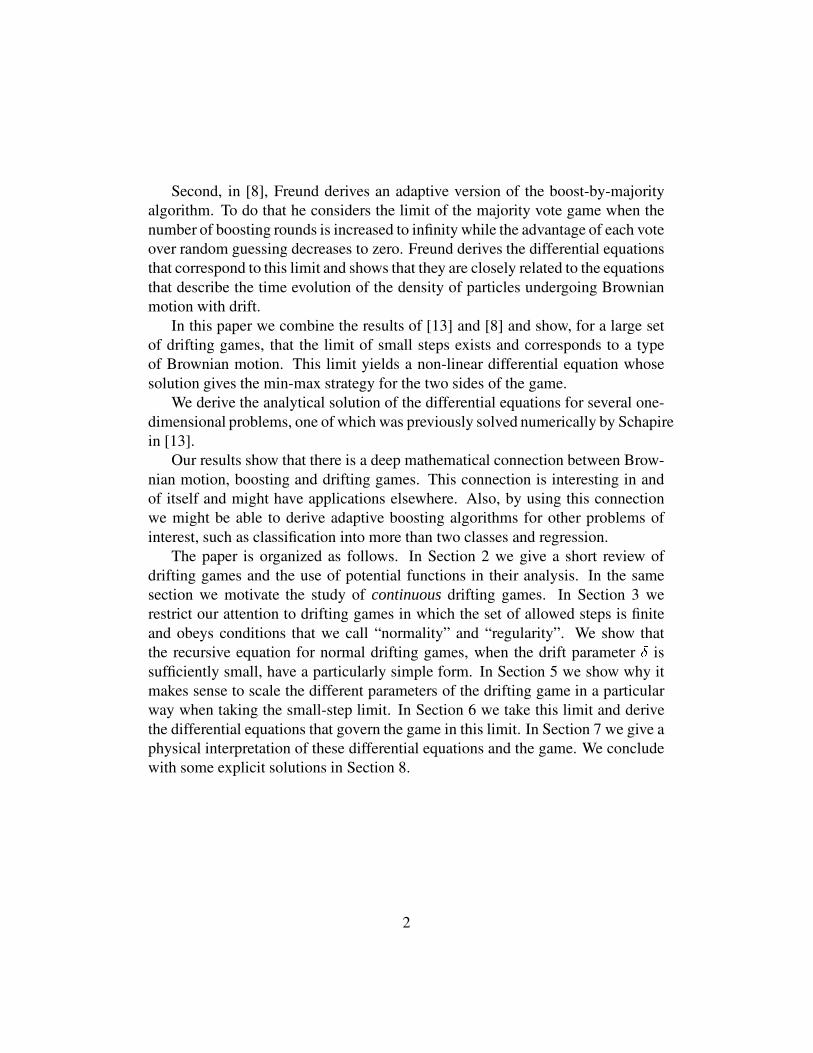
Figure 2: The potential ����������� for the square loss ������ � � � .ferent times. The step functions represent the corresponding solutions for Equa-tion (5) with step size � � � <� . We also computed � for the two loss functions�A@ � C � � � and � @�� C � ��� @ � � ��� C (see Figures 2 and 3) which maybe of interestin a regression framework. In these cases Equation (20) can still be expressedanalytically in terms of error functions but the resulting expressions are long andcomplex. Instead, we have chosen to calculate the potential function by numericalintegration.

9 Numerical solutions for ��� �In higher dimensions as well as for loss functions which do not have the nice sym-metries of the examples in the previous section we will have to resort to numericalsolutions of the partial differential Equation (12).

19

−5.0 −4.0 −3.0 −2.0 −1.0 0.0 1.0 2.0 3.0 4.0 5.0s

0.0

0.2

0.5

0.8

1.0

φ(s,τ) τ=0.0τ=0.5τ=0.9τ=0.99

Figure 3: The potential ����������� for the loss ������ ������� ��� � � ! � .

20

To discuss some of the inherrent problems with such an approach we considerthe regular lattice (4) in � � . For this case, we have � 4 � � � � 4 � �

and � 4 4 ��� �� 4

� . Numerical packages will usually solve PDEs in forward time startingfrom a given initial condition. Hence, we define the function � @ ��� C � � @ ��� � � Cwith the initial condition � @ � � C � �A@ C . Writing the components of positionvectors as � @�� � � C and choosing the � � norm, eq. (12) becomes� � @ � � C� � � �

�� � � @ ��� C� � � = �

�� � � @ ��� C� � �

� �

���� � � � @ ��� C� � � � = � � � @ ��� C� � � � (20)

To be specific, we will specialize to a loss function � @ C which equals 1 if the point is closest to 4 and 0 if it is closer to � or �� than to 4 . The region with �A@ C ���is a wedge of � � degress width, centered at the origin � �

and symmetric to theaxis � � �

. This problem corresponds to boosting for classification problems withthree possible labels as described by Schapire in [13]. The initial condition for thePDE reads

� @ � � C � %�� ' � � � � � � (21)Before attempting a numerical solution, we have to deal with two questions: Howto choose appropriate boundary conditions and how to deal with the nonsmoothinitial conditions given by (21).

Numerical solutions of the PDE must obviously be constrained to some finiteregion �� � � . The choice of this region has to be supplemented by a sensible apriori specification of how the solution should behave at the artificial boundaries� � of the region � . Simply fixing � @ ��� C for . � � for all times � to its initialvalues (corresponding to (21)) seems to create a rather crude approximation tothe real problem defined on the entire � � . We have rather chosen a boundarycondition which models a situation where the diffusing “sheep” are not allowedto leave or enter the region � , i.e. the local probability flow at the boundary isrequired to be zero. Gardiner [10] shows that these reflecting boundary conditionsas specified for the backward equation (12) are mathematically expressed as

@ C � � � @ ��� C � �for . � � (22)

@ C is a vector perpendicular to the boundary at �� .The second problem that prevents us from a straightforward numerical solu-

tion of (20) is the discontinuity of the initial condition (21) at the line � � � � � � � . (22) belongs to the class of “natural boundary conditions”.

21

This creates infinite spatial derivatives at time �8� �. Since it would require infi-

nite precision in discretizing the PDE at this line, any finite spatial discretizationmay create uncontrollable artifacts and errors in the numerical solution. Hence,we have chosen to replace the original problem (21) by the smoothed version

� @ � � C � % �� �� ' � � � � � � � (23)

which is based on a smoothed step function defined by % �� �� � 4�@ � = � � @�� ��� C�C .

The parameter � measures the typical lengthscale over which the step functionsmoothly varies from 0 to 1. The original % � is recovered in the limit � � �

.This approach seems reasonable by the fact that the continuum limit of the PDEis understood as an approximation for a game with finite step size. Hence, asensible choice is to take � small compared to the step size of the original sheepgame. We have solved the PDE (20,23) for

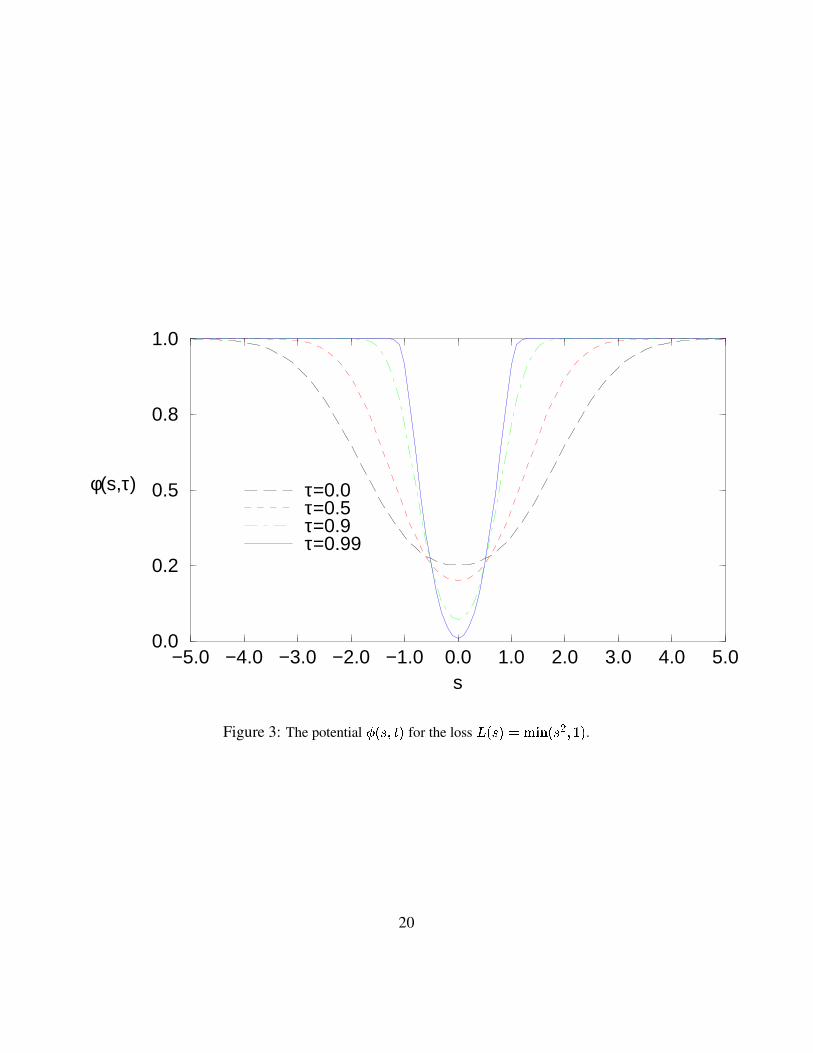
� � � on the square � � � ��� � � � �using the FLEXPDE package � . We used a basic and straightforward definition ofour problem as described in the code given in Appendix A. In order to obtaina reasonable approximation within the limits of the demo software we use therather large smoothing parameter � � � for the initial condition (23). The resultsfor the potential � @ ��� C for times � � � (the initial loss) and � � �

are shown inFigure 4. The two straight lines in the � � � plane show the function � � � � � � � ,where the unsmoothed loss function (21) jumps from � � �

to � � � . Sinceby symmetry, the potential comes out symmetric with respect to the axis � � �(i.e. � @ � � � � ��� C � � @�� � � ��� C ), we have displayed � @�� � � ��� � � C for � � �

and� @�� � � ��� � � C for � � �only. As expected from the relation (15), as the time� decreases, the potential becomes further smoothed. This effect is also visible

in the contour plots (Figs. 5,6) where we have also shown the weight vectors(perpendicular to the lines of constant potential) as arrows. At � � �

, the potentialis less steep than for � � � .

A FLEXPDE code

TITLE ’ brownboost’VARIABLES�

FLEXPDE is a commercial PDE solver distributed by PDE-solutions Inc. It is based ona finite element approach which automatically creates a problem specific mesh over the spatialdomain. Functions are polynomially interpolated over each mesh cell. We used a demo versionof FLEXPDE which can be downloaded from http://www.pdesolutions.com

22

−5

0

5

−5

0

50

0.2

0.4

0.6

0.8

1

x

φ(x,y,t=1)

y

φ(x,y,t=0)

Figure 4: � � � ����� for � � ! (only ��� $ shown) and � � $ (only ��� $ shown) for the

two dimensional problem. The missing parts for both functions follow by symmetry.

23

−5 −4 −3 −2 −1 0 1 2 3 4 5−5

−4

−3

−2

−1

0

1

2

3

4

5

x

y

Figure 5: Contour plot of the potential (initial loss) ��� �*��� � ! � for the two dimensional

problem together with the weightvectors � � � �*��� � ! � ����� � �*��� � ! � .Psi(range=0,1)DEFINITIONSlam=1.0L=5INITIAL VALUESPsi=0.5*ERF((y-ABS(x)/sqrt(3))/lam)+0.5EQUATIONSdt(psi)= 0.25*div(grad(Psi))- Magnitude(grad(psi))BOUNDARIESregion 1 ’box’start(-L,-L)NATURAL(Psi)=0 line to (L,-L)

24

−5 −4 −3 −2 −1 0 1 2 3 4 5−5

−4

−3

−2

−1

0

1

2

3

4

5

x

y

Figure 6: Contour plot of the potential ��� �*��� � $ � for the two dimensional problem

together with the weightvectors � � � �*��� � $ � ����� � �*��� � $ � .

25

NATURAL(Psi)=0 line to (L,L)NATURAL(Psi)=0 line to (-L,L)NATURAL(Psi)=0 line to finishTIME0 to 1 by 0.01PLOTSfor t=0.0 by 0.5 to 1.0CONTOUR(Psi) GrayTABLE(Psi) Points = 51END

References

[1] Javed Aslam. Noise Tolerant Algorithms for Learning and Searching. PhDthesis, Massachusetts Institute of Technology, 1995. MIT technical reportMIT/LCS/TR-657.

[2] Javed A. Aslam and Aditi Dhagat. Searching in the presence of linearlybounded errors. In Proceedings of the Twenty Third Annual ACM Symposiumon Theory of Computing, May 1991.

[3] Javed A. Aslam and Aditi Dhagat. On-line algorithms for -coloring hyper-graphs via chip games. Theoret. Comput. Sci., 112(2):355–369, 1993.

[4] Leo Breiman. Probability. SIAM, classics edition, 1992. Original editionfirst published in 1968.

[5] Nicolo Cesa-Bianchi, Yoav Freund, David P. Helmbold, and Manfred K.Warmuth. On-line prediction and conversion strategies. Machine Learning,25:71–110, 1996.

[6] Aditi Dhagat, Peter Gacs, and Peter Winkler. On playing “twenty questions”with a liar. In Proceedings of the Third Annual ACM-SIAM Symposium onDiscrete Algorithms (Orlando, FL, 1992), pages 16–22, New York, 1992.ACM.

[7] Yoav Freund. Boosting a weak learning algorithm by majority. Informationand Computation, 121(2):256–285, 1995.

26

[8] Yoav Freund. An adaptive version of the boost by majority algorithm. Ma-chine Learning, 43(3):293–318, June 2001.

[9] Yoav Freund and Robert E. Schapire. A decision-theoretic generalization ofon-line learning and an application to boosting. Journal of Computer andSystem Sciences, 55(1):119–139, August 1997.

[10] C.W. Gardiner. Handbook of Stochastic Methods. Springer Verlag, 2ndedition, 1985.

[11] Llew Mason, Jonathan Baxter, Peter Bartlett, and Marcus Frean. Functionalgradient techniques for combining hypotheses. In Alexander J. Smola, Pe-ter J. Bartlett, Bernhard Scholkopf, and Dale Schuurmans, editors, Advancesin Large Margin Classifiers. MIT Press, 1999.

[12] Llew Mason, Jonathan Baxter, Peter Bartlett, and Marcus Frean. Boostingalgorithms as gradient descent. In Advances in Neural Information Process-ing Systems 12, 2000.

[13] Robert E. Schapire. Drifting games. Machine Learning, 43(3):265–291,June 2001.

[14] Robert E. Schapire and Yoram Singer. Improved boosting algorithms usingconfidence-rated predictions. Machine Learning, 37(3):297–336, December1999.

[15] Glenn Shafer and Vladimir Vovk. Probability and Finance, it’s only a game!Wiley, 2001.

[16] Joel Spencer. Ten Lectures on the Probabilistic Method. Society for Indus-trial and Applied Mathematics, Philadelphia, 1987.

[17] Joel Spencer. Ulam’s searching game with a fixed number of lies. Theoret.Comput. Sci., 95(2):307–321, 1992.

[18] V. G. Vovk. A game of prediction with expert advice. Journal of Computerand System Sciences, 56(2):153–173, April 1998.

27