Continuity and Smoothness Properties ofNonlinear Optimization-Based Feedback Controllers

Benjamin J. Morris, Matthew J. Powell, Aaron D. Ames

Abstract— Online optimization-based controllers are becom-ing increasingly prevalent as a means to control complex high-dimensional nonlinear systems, e.g., bipedal and humanoidrobots, due to their ability to balance multiple control objectivessubject to input constraints. Motivated by these applications,the goal of this paper is to explore the continuity and smooth-ness properties of feedback controllers that are formulated asquadratic programs (QPs). We begin by drawing connectionsbetween these optimization-based controllers and a family ofperturbed nonlinear programming problems commonly studiedin operations research. With a view towards robotic systems,some existing results on perturbed nonlinear programmingproblems are extended and specialized to address conditionsthat arise when quadratic programs are used to enforce theconvergence of control Lyapunov functions (CLFs).

The main result of this paper is a novel set of conditions onthe continuity of QPs that can be used when a subset of theconstraints vanishes. A simulation study of position regulationin the compass gait biped demonstrates how the new conditionsof this paper can be applied to more complex robotic systems.

I. INTRODUCTION

With the rise in computation power and the ubiquity ofpowerful and inexpensive mobile processors, there is an everincreasing ability to realize implicitly defined optimization-based controllers in real-time. The benefits of controllers ofthis form have been known for some time [19], especiallyin the context of model predictive control (MPC) of linearsystems [13], [14] (and, in limited scope, nonlinear systems[16]). Yet the increase in mobile computation power pointsto the ability to extend these benefits to the real-time controlof general nonlinear systems where the feedback controlleritself is implemented as the solution to a nonlinear optimiza-tion problem, i.e., a nonlinear programming problem, at eachtime step. The ability to characterize controllers of this formwould have a variety of unique benefits: a large numberof control objectives could be simultaneously considered,physical constraints (e.g., torque bounds and state con-straints) could be dynamically balanced against these controlobjectives, and trajectory planning could be subsumed intothe real-time control process. These advantages are especiallyacute in the context of nonlinear systems, for which roboticsystems provides a quintessential example.

Benjamin J. Morris is a consultant at Matrix Computing and is analumnus of the EECS:Systems department of the University of Michi-gan {benmorris@matrixcomputing.com, morrisbj@umich.edu}, Matthew J.Powell is with the the School of Mechanical Engineering, and Aaron D.Ames is with the School of Mechanical Engineering and the School ofElectrical and Computer Engineering, Georgia Institute of Technology, At-lanta, GA 30332 {mjpowell@gatech.edu,ames@gatech.edu} The researchof Matthew J. Powell and Aaron D. Ames is supported by NSF CPS award1239055.

α

ph2

pv2q1

q2

lcl

COM

V. EXPERIMENTAL RESULTS AND FUTURE WORK

The proposed MPC-based controller for bipedal roboticwalking was implemented in C++ on the Durus robot usingan internal dynamics model integration method to convertthe feedback linearization torques into position and velocitycommands [4]. Data from an experiment in which the robotsuccessfully completed three laps around the room (63 steps)is shown in Figure 7. The average phase portraits fromexperiment agree quite well with the corresponding phaseportraits from simulation, presented earlier in Figure 1. Inthe experiment phase portrait, bi-periodicity is apparent: thisis due to the fact that the boom which supports Durus doesnot entirely enforce planar motion. A video of the experimentis available online http://youtu.be/OG-WIfWMZek.

Formal stability of the hybrid periodic orbit as a resultof the proposed MPC control approach is a prime focusof current research. Existing methods of proving stabilityof the orbit rely on exponential stability of the continuous-time controller, and to the authors’ knowledge, a proof ofstability under nontrivial torque saturation is still an openproblem. To address the hybrid stability problem, it will beimportant to note existing methods of proving stability ofMPC controllers, such as those described in [14], imposeconditions on a terminal cost ηTNPεηN . Zero dynamics playa large part in the current work. Increasing the dimensionalityof the zero dynamics (such as going to 3D) poses significantchallenges that need to be addressed. A note on the method:the proposed MPC problem is (currently) not intended toreplace the nonlinear optimization that produces the nominalgait. Associated with the nominal gait is a feedforwardtorque profile; deviations from these nominal torques willnecessarily change the gait. The standard approach wouldbe to re-solve the constrained nonlinear optimization for adifferent gait with lower torque bounds; however, this comeswith its own challenges and it has to be done offline. Instead,the current MPC formulation intends to be a step towardshandling (reasonable) torque bounds at the online controlimplementation level, and thus, relieve some of the burdenof the offline optimization.

REFERENCES

[1] A. D. Ames. Human-inspired control of bipedal walking robots.Automatic Control, IEEE Transactions on, 2014.

[2] A. D. Ames, K. Galloway, and J. W. Grizzle. Control lyapunovfunctions and hybrid zero dynamics. In Decision and Control (CDC),2012 IEEE 51st Annual Conference on, 2012.

[3] A. D. Ames and M. Powell. Towards the unification of locomotionand manipulation through control lyapunov functions and quadraticprograms. In Control of Cyber-Physical Systems, Lecture Notes inControl and Information Sciences. 2013.

[4] E. Cousineau and A. D. Ames. Realizing underactuated bipedalwalking with torque controllers via the ideal model resolved motionmethod. IEEE International Conference on Robotics and Automation(ICRA), 2015.

[5] J. Deng, V. Becerra, and R. Stobart. Input constraints handling in anmpc/feedback linearization scheme. Int. J. Appl. Math. Comput. Sci.,2009.

[6] R. A. Freeman and P. V. Kokotovic. Robust Nonlinear Control Design.Birkhauser, 1996.

[7] K. S. Galloway, K. Sreenath, A. D. Ames, and J. W. Grizzle.Torque saturation in bipedal robotic walking through control lyapunovfunction based quadratic programs. CoRR, abs/1302.7314, 2013.

−0.4 −0.2 0 0.2 0.4 0.6−3

−2

−1

0

1

2

3

Angle (rad)

Velocity

(rad/s)

θsa θsk θsh θnsh θnsk

0 0.5 1 1.5 2 2.5−0.6

−0.4

−0.2

0

0.2

0.4

0.6

0.8

Time (s)

Angle

(rad)

θa

skθa

shθa

nshθa

nsk

θd

skθd

shθd

nshθd

nsk

Fig. 7. Results from experiment of the proposed MPC-based QP for roboticwalking with Durus (right), showing phase portraits (top left) for 63 steps ofwalking together with a darker averaged phase portrait and position trackingerrors (bottom left) over a select 4 steps in the same experiment.

[8] G. Garofalo, C. Ott, and A. Albu-Schaffer. Walking control of fullyactuated robots based on the bipedal slip model. In Robotics andAutomation (ICRA), 2012 IEEE International Conference on, 2012.

[9] J. W. Grizzle and E. R. Westervelt. Hybrid zero dynamics of planarbipedal walking. In Analysis and Design of Nonlinear Control Systems.2008.

[10] S. Kajita, F. Kanehiro, K. Kaneko, K. Fujiwara, K. Harada, K. Yokoi,and H. Hirukawa. Biped walking pattern generation by using previewcontrol of zero-moment point. In Robotics and Automation, 2003.Proceedings. ICRA ’03. IEEE International Conference on, 2003.

[11] X.-B. Kong, Y. jie Chen, and X. jie Liu. Nonlinear model predictivecontrol with input-output linearization. In Control and DecisionConference (CCDC), 2012 24th Chinese, 2012.

[12] S. Kuindersma, F. Permenter, and R. Tedrake. An efficiently solvablequadratic program for stabilizing dynamic locomotion. CoRR, 2013.

[13] M. J. Kurtz and M. A. Henson. Input-output linearizing control ofconstrained nonlinear processes. Journal of Process Control, 1997.

[14] D. Q. Mayne, J. B. Rawlings, C. V. Rao, and P. O. M. Scokaert.Survey constrained model predictive control: Stability and optimality.Automatica, 2000.

[15] B. Morris and J. Grizzle. A restricted poincar’e; map for determiningexponentially stable periodic orbits in systems with impulse effects:Application to bipedal robots. In Decision and Control, CDC-ECC.44th IEEE Conference on, 2005.

[16] B. Morris, M. Powell, and A. Ames. Sufficient conditions for thelipschitz continuity of qp-based multi-objective control of humanoidrobots. In IEEE Conference on Decision and Control (CDC), 2013.

[17] R. M. Murray, Z. Li, and S. S. Sastry. A Mathematical Introductionto Robotic Manipulation. CRC Press, Boca Raton, 1994.

[18] M. Posa and R. Tedrake. Direct trajectory optimization of rigid bodydynamical systems through contact. In Algorithmic Foundations ofRobotics X, Springer Tracts in Advanced Robotics. 2013.

[19] J. Pratt, J. Carff, and S. Drakunov. Capture point: A step towardhumanoid push recovery. In 6th IEEE-RAS International Conferenceon Humanoid Robots, Genoa, Italy, 2006.

[20] S. S. Sastry. Nonlinear Systems: Analysis, Stability and Control.Springer, New York, 1999.

[21] M. W. Spong and M. Vidyasagar. Robotic Dynamics and Control.John Wiley and Sons, New York, NY, 1989.

[22] B. Stephens and C. Atkeson. Push recovery by stepping for humanoidrobots with force controlled joints. In International Conference onHumanoid Robots, Nashville, Tennessee, 2010.

Fig. 1. (Left) The planar two-link compass-gait walker is a simple robot thatcan be used to illustrate the smoothness properties of feedback controllersimplemented via constrained optimization problems (nonlinear programs).(Right) The bipedal robot DURUS is a complex nonlinear system; workingto implement the control-via-optimization methods on DURUS and similarrobots has motivated the development and understanding of the formalresults presented.

There has been a recent surge in the use of optimization-based feedback controllers, and specifically quadratic pro-gram based (QP) controllers, in the robotics domain due tothe aforementioned benefits. Beginning at the level of centerof mass and foot placement planning, the fact that undercertain stringent conditions the center of mass dynamicsbecome linear allows for the formulation of a QP basedplanner [20]. This observation can be coupled with the factthat the equations of motion are affine in torque to achievewhole-body behaviors on humanoid robots [12], [21], [22],[24]. Coming from the perspective of nonlinear control ofrobotic systems, QP controllers can also be formulated toexploit the fact that control Lyapunov functions (CLF) forthese systems are, again, affine in torque [9]. This frameworkwas utilized, with the addition of torque bounds, to realizebipedal robotic walking [3], [5], [10] (see videos of thebehavior at [1]). Building upon this observation, this method-ology was extended to allow for the balancing of multiplecontrol objectives subject to force and torque constraints [2],was recently realized onboard and in real-time on prosthesis[25], and has been utilized to achieve robotic walking vianonlinear MPC related concepts [17]. Yet in all of the aboveapplications, the authors have found few formal results on thecontinuity and smoothness properties of these optimization-based controllers. Except in special cases, establishing theseproperties is a difficult problem due to the lack of a closedfrom expression for the resulting controllers.

In this paper we investigate the smoothness properties

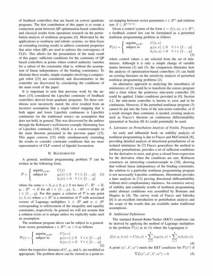
of feedback controllers that are based on convex quadraticprograms. The first contribution of this paper is to create aconnection point between QP optimization-based controllersand classical results from operations research on the pertur-bation analysis of nonlinear programs [4]. Motivated by theapplications to nonlinear and robotic systems, we then focuson extending existing results to address constraint propertiesthat arise when QPs are used to enforce the convergence ofCLFs. This allows for the presentation of the main resultof this paper: sufficient conditions for the continuity of QPbased controllers at points where control authority vanishesfor a subset of the constraints (that is, without the assump-tion of linear independence of the binding constraints). Toillustrate these results, simple examples involving a compass-gait robot [23] are considered, and discontinuities in thecontroller are discovered by considering the conditions ofthe main result of the paper.

It is important to note that previous work by the au-thors [15] considered the Lipschitz continuity of feedbackcontrollers derived from quadratic programs. Yet these con-ditions were incorrectly stated; the error resulted from anincorrect assumption that a single-valued mapping that isboth upper and lower Lipschitz continuous is Lipschitzcontinuous (in the traditional sense)—an assumption thatdoes not hold, in general. This was discovered by the authorsthrough the Robinson’s well-known example illustrating lossof Lipschitz continuity [18] which is a counterexample tothe main theorem presented in the previous paper [15].This paper corrects [15] while simultaneously extendingthe results to consider constraint conditions that are morerepresentative of CLF control of bipedal locomotion.

II. BACKGROUND

A general, nonlinear programming problem P can bewritten in the following form,

P =

argminx∈Rn C(x)subject to gi(x) ≤ 0 ∀ i ∈ {1 . . . p}

hi(x) = 0 ∀ i ∈ {1 . . . q}(1)

where for some n > 0, p ≥ 0, q ≥ 0 we have C : Rn → R,gi : Rn → R for all i ∈ {1 . . . p}, hi : Rn → R for alli ∈ {1 . . . q}. For this paper, a solution of P is any point(x, λ,w) where x ∈ Rn is a minimizer of P with associatedvectors of Lagrange multipliers λ ∈ Rp and w ∈ Rq

corresponding to enforcement of the inequality and equalityconstraints, respectively. In general we will not assume thata solution exists or is unique unless we explicitly make suchan assumption.

The nonlinear program above can be subject to a general-form vector perturbation ε ∈ Rm, m > 0 as follows

P(ε) =

argminx∈Rn C(x, ε)subject to gi(x, ε) ≤ 0 ∀ i ∈ {1 . . . p}

hi(x, ε) = 0 ∀ i ∈ {1 . . . q}(2)

where the respective domains of C, gi, and hi are modified asappropriate. The problem above can be viewed as a point-to-

set mapping between vector parameters ε ∈ Rm and solutionsets X ⊂ Rn+p+q .

Given a control system of the form x = f(x, u), x ∈ Rm,a feedback control law can be formulated as a perturbednonlinear programming problem as follows

P(x) =

argminu∈Rn C(u, x)subject to gi(u, x) ≤ 0 ∀ i ∈ {1 . . . p}

hi(u, x) = 0 ∀ i ∈ {1 . . . q}(3)

where control values u are selected from the set of min-imizers. Although it is only a simple change of variablenames between (2) and (3), the comparison illustrates howthe analysis of optimization-based controllers (3) can buildon existing literature on the sensitivity analysis of perturbednonlinear programming problems (2).

An alternative approach to analyzing the smoothness ofminimizers of (3) would be to transform the convex programinto a form where the pointwise min-norm controller [9]could be applied. Under conditions provided in [9], Section4.2, the min-norm controller is known to exist and to becontinuous. However, if the perturbed nonlinear program (3)cannot be put into the form of the min-norm controller, or ifa result stronger than continuity is needed, existing analysissuch as Fiacco’s theorem on continuous differentiability(presented in Section III-A) could potentially be used.

A. Literature on Perturbation Analysis of Nonlin. Programs

An early and influential book on stability analysis ofnonlinear programming is due to Fiacco and McCormick [8],providing detailed analysis of directional perturbations of anisolated minimizer. In [7] Fiacco generalizes the method toarbitrary perturbations, provides a set of sufficient conditionsfor the derivative to exist, and gives a closed form expressionfor the derivative when the conditions are met. Robinsonconstructs an interesting counterexample in [18], showingthat without linear independence of the binding constraints,the solution to a particular nonlinear programming programis not necessarily Lipschitz continuous. Jittorntrum providesa later analysis in [11] proving directional differentiabilitywithout strict complementary slackness. An extensive surveyof stability and continuity results of nonlinear programmingunder abstract conditions was assembled by Bonnans andShapiro in [4]. The survey work of Fiacco and Ishizuka[6] is an excellent introduction to perturbation analysis andthe scope of the results that are available under traditionalassumptions.

B. Additional Definitions

The standard Karush-Kuhn-Tucker (KKT) conditions canbe derived by applying the method of Lagrange multipliersto the problem P(x) as in (3) where the Lagrangian is

L(x, u, λ, w) = C(u, x) +

p∑i=1

λigi(u, x) +

q∑i=1

wihi(u, x).

(4)A point (u∗, λ∗, w∗) meets the KKT conditions for P(x∗) if

∇L(x∗, u∗, λ∗, w∗) = 0 (5)

andhi(u

∗, x∗) = 0 for i ∈ {1 . . . q}gi(u

∗, x∗) ≤ 0 for i ∈ {1 . . . p}λ∗i gi(u

∗, x∗) = 0 for i ∈ {1 . . . p}λ∗i ≥ 0 for i ∈ {1 . . . p}.

(6)

A point (u∗, λ∗, w∗) satisfies the linear independenceconstraint qualification (LICQ) for P(x∗) (or, in differentterminology, is said to be regular) if the gradients of theactive constraints of P(x∗) are linearly independent. Thatis, the matrix[ ∂

∂uhi(u∗, x∗) ∀ i ∈ {1 . . . q}

∂∂ugi(u

∗, x∗) ∀ i s.t. gi(u∗, x∗) = 0

](7)

has full row rank.A point (u∗, λ∗, w∗) satisfies complementary slackness for

P(x∗) if λ∗i gi(u∗, x∗) = 0 for each i and satisfies strict

complementary slackness if there does not exist any i forwhich both λ∗i = 0 and gi(u∗, x∗) = 0.

A point (u∗, λ∗, w∗) satisfies the second order sufficientconditions for P(x∗) if

i) the functions C(u, x), gi(u, x) for i ∈ {1 . . . p}, andhi(u, x) for i ∈ {1 . . . q} are twice continuously differ-entiable in u, for u in an open neighborhood of u∗ andx = x∗ fixed

ii) the point (u∗, λ∗, w∗) satisfies the KKT conditions forP(x∗)

iii) for any y 6= 0 satisfyingyT ∂

∂ugi(u∗, x∗) ≤ 0 for all i where λ∗i = 0

yT ∂∂ugi(u

∗, x∗) = 0 for all i where λ∗i > 0

yT ∂∂uhi(u

∗, x∗) = 0 for i ∈ {1 . . . p}the following inequality holds:

yT∇2L(x∗, u∗, λ∗, w∗)y > 0,

where the Hessian matrix operator, denoted ∇2, is takenwith respect to the variable u.

A function f : Rm → Rn is Lipschitz continuous atx ∈ Rm if there exists values δ > 0 and L > 0, bothperhaps dependent on the value of x, such that for allx1, x2 ∈ Bδ(x) ⊂ Rm, ‖f(x2)− f(x1)‖ ≤ L‖x2 − x1‖.

III. TWO RESULTS FROM THE LITERATURE ONPERTURBATION ANALYSIS OF CONVEX PROGRAMS

Perturbed convex nonlinear programs such as (2) havebeen analyzed extensively in the literature. This sectionreviews two existing results that are relevant in analyzing(3) as a feedback controller. The first result below providesconditions under which the minimizer is unique and dif-ferentiable. The second provides an example showing thatunder a different set of conditions, a unique minimizer isnot necessary Lipshitz continuous.

A. Sufficient Conditions for Differentiability

The following theorem is from Fiacco [7] Theorem 2.1and has been modified to fit the notation of this paper.

Theorem 1: [Differentiability of the Minimizer]Given a perturbed nonlinear programming problem P(x) asin (3) and a parameter vector x∗ = 0, suppose the followingH1.1) the functions C(u, x), gi(u, x) for i ∈ {1 . . . p}, and

hi(u, x) for i ∈ {1 . . . q} are twice continuouslydifferentiable in (u, x) in an open neighborhood of(u∗, 0)

H1.2) there exists a point (u∗, λ∗, w∗) that satisfies thesecond order sufficient condition of P(x) at x∗ = 0

H1.3) the point (u∗, λ∗, w∗) satisfies the linear indepen-dence constraint qualification of P(x) at x∗ = 0

H1.4) the point (u∗, λ∗, w∗) satisfies strict complementaryslackness for P(x) at x∗ = 0

thena) u∗ is an isolated local minimizer of P(x) at x∗ = 0b) for x in a neighborhood of 0 there exist continuously

differentiable functions u(x), λ(x), and w(x) (withu(0) = u∗, λ(0) = λ∗, and w(0) = w∗) such that u(x)is an isolated local minimizer of P(x), with associatedunique Lagrange multiplier vectors λ(x) and w(x)

c) the point (u(x), λ(x), w(x)) satisfies strict complemen-tary slackness and the linear independence constraintqualification for P(x) for x in a neighborhood of 0

B. Robinson’s Counterexample

The following example, presented by Robinson in [18],shows that even under strict convexity, a perturbed quadraticprogram might result in solutions that are non-Lipschitz withrespect to perturbations.

Consider the following strictly convex quadratic program

P(x) =

{argminu∈R4

12u

Tu

subject to A(x)u ≥ b(x)(8)

where x = (x1, x2) ∈ R2 and

A(x) =

0 −1 1 00 1 1 0−1 0 1 0

1 0 1 x1

b(x) =

111

1 + x2

. (9)

Note that for 0 < x1, 0 ≤ x2 ≤ 12x

21, the unique minimizer

can be computed in closed form

u(x) = (0, 0, 1, 0)T +x2x1

(0, 0, 0, 1)T , (10)

and for x1 = x2 = 0 the solution is

u(x) = (0, 0, 1, 0)T . (11)

Although we have existence and uniqueness of the min-imizer u(x) for any value of x = (x1, x2), the minimizeritself is not Lipschitz continuous in any open set containing(x1, x2) = (0, 0).

IV. APPLICATION TO FEEDBACK VIA CONTROLLYAPUNOV FUNCTIONS

Given an affine nonlinear control system

x = f(x) + g(x)u (12)

with x ∈ Rm, u ∈ Rn, consider a set of control objectives,each encoded as the zeroing of a smooth scalar outputfunction yi : Rm → R.

A. Input-Output Linearization and RES-CLFs

If we have a set of n outputs and the correspondingvector y(x) = (y1(x), . . . , yn(x))T has a well-defined vectorrelative degree, then feedback linearization can be applied.Assume that our vector of outputs has vector relative degree2. The control law

u(x) = LgLfy(x)−1(µ− L2fy(x)) (13)

when applied to the dynamics (12) results in the lineardecoupled input-output system

y = µ (14)

for any µ ∈ Rn. Or, equivalently

η =

[0 I0 0

]︸ ︷︷ ︸

F

η +

[0I

]︸ ︷︷ ︸G

µ. (15)

for η = (yT , yT )T . With this form, we can now construct aRES-CLF following the steps given in [3], [5].

B. Constructing a Rapidly Exponentially Stabilizing ControlLyapunov Function (RES-CLF)

For the system in (15), a continuously differentiable func-tion Vε : X → R is a rapidly exponentially stabilizingcontrol Lyapunov function (RES-CLF) if there exist positiveconstants c1, c2, c3 > 0 such that for all 0 < ε < 1,

c1‖η‖2 ≤ Vε(η) ≤ c2ε2‖η‖2, (16)

infµ∈Rn

[LFVε(η) + LGVε(η)µ+

c3εVε(η)

]≤ 0, (17)

for all η ∈ X . A RES-CLF for the outputs η can beconstructed via:

Vε(η) := ηT IεPIε︸ ︷︷ ︸Pε

η, Iε := diag

(1

εI, I

), (18)

where I is the identity matrix and P = PT > 0 solvesthe the continuous time algebraic Riccati equations (CARE)FTP + PF − PGGTP + Q = 0 for Q = QT > 0. Thetime-derivative of (18) is given by

Vε(η) = LFVε(η) + LGVε(η)µ, (19)

where

LFVε(η) = ηT (FTPε + PεF )η, (20)

LGVε(η) = 2ηTPεG, (21)

are the Lie derivatives of Vε(η) along the vector fields F andG. As noted in [3] a RES-CLF can be realized by includingthe inequality constraint (17) in a feedback controller basedon nonlinear programming.

P(η) =

{argminµ∈Rn

12µ

Tµ

subject to LGVε(η)µ ≤ − c3ε Vε(η)− LFVε(η)(22)

C. Conditions for Continuously Differentiable Minimizers ofthe CLF-QP

The following theorem provides sufficient conditions forthe unique minimizer of (22) to be continuously differen-tiable

Theorem 2: Consider the parameterized nonlinear pro-gram (22) at η = η∗. Suppose that for this vector thefollowing hold:H2.1) LGVε(η), Vε(η), LFVε(η) and are twice continuously

differentiable in an open neighborhood containing η∗

H2.2) there exists a point (µ∗, λ∗, w∗) that satisfies thelinear independent constraint qualification of P(η∗).

H2.3) the point (µ∗, λ∗, w∗) satisfies complementary slack-ness holds for P(η∗)

Then there exists a continuously differentiable function µ(η)defined on an open neighborhood containing η∗ such that forall η in this neighborhood µ(η) is the unique minimizer ofP(η).

Proof: Note that the trivial quadratic cost functionimplies that the second order sufficient condition holds, andapply Theorem 1.

Note that for a CLF-QP as in (22) the theorem aboveshows that the solution µ(η) is continuously differentiablewhenever LGVε(η) has full row rank and strict complemen-tary slackness is satisfied. Most notably, this breaks downat V (η) = ηTPεη = 0, when η = 0 and LGVε(η) = 0. Theconvergence constraint becomes

LGVε(0)µ ≤ −c3εVε(0)− LFVε(0) (23)

or, equivalently0µ = 0. (24)

The vector of zeros means that the linear independent con-straint qualification breaks down. The main theorem of thepaper which is presented in the following section provides analternative set of conditions that does not require the linearindependent constraint qualification, and can thus be used toanalyze constraints such as (23).

V. CONTINUITY UNDER VANISHING CONSTRAINTS

This section contains the main result of the paper, es-tablishing sufficient conditions under which continuity ofthe minimizer (but not necessarily Lipschitz continuity ordifferentiability) can be recovered when the linear indepen-dent constraint qualification does not hold. To demonstratethe application of the main theorem, Section VI provides asimple case study under which the conditions Theorem 1

fail, but the continuity of the minimizer can still be provenusing the main theorem (Theorem 3).

A. Properties of Solutions to Nonlinear Programs

The following propositions provide useful relationshipsbetween nonlinear programs that share the same objectivefunction.

Proposition 1: Given a pair of nonlinear programs

P0 =

{argmin f(u)subject to u ∈ S0

(25)

P1 =

{argmin f(u)subject to u ∈ S1

(26)

with S0 ⊂ S1 ⊂ D ⊂ Rn, n ≥ 1, f : Rn → R, assume thatP0 and P1 have minimizers (that are possibly non-unique),designated u∗0 and u∗1 respectively. Then f(u∗0) ≥ f(u∗1)

Proof: Suppose the alternative, that under the givenassumptions f(u∗0) < f(u∗1). Then, u∗1 could not be aminimizer of P1 because u∗0 ∈ S0 ⊂ S1 is a feasible pointof P1 with a lower value for the objective function thanu∗1 provides. However, it is given that u∗1 is a minimizer.Thus the alternative must be false, thus proving the claim bycontradiction.

Proposition 2: Given three nonlinear programs:

PS =

{argmin f(u)subject to u ∈ ΦS

(27)

P =

{argmin f(u)subject to u ∈ Φ

(28)

PB =

{argmin f(u)subject to u ∈ ΦB

(29)

with ΦS ⊂ Φ ⊂ ΦB ⊂ D ⊂ Rn, n ≥ 1 where f : D → R,suppose that

i) PS, P and PB have unique minimizers, designated u∗S,u∗, and u∗B respectively.

ii) There exists some c > 0 such that for any v1, v2 ∈ D,

c‖v1 − v0‖2 ≤ |f(v1)− f(v0)| (30)

iii) The function f is Lipschitz continuous on D. That is,there exists L ≥ 0 such that for any v0, v1 ∈ D,

|f(v1)− f(v0)| ≤ L‖v1 − v0‖ (31)

Then‖u∗ − u∗S‖2 ≤

L

c‖u∗S − u∗B‖. (32)

Proof: Apply Proposition 1 twice to see

f(u∗S) ≥ f(u∗) ≥ f(u∗B). (33)

By the second order growth bound (ii) we have that

c‖u∗S − u∗‖2 ≤ f(u∗S)− f(u∗) (34)

Note that by (33)

f(u∗S)− f(u∗) = f(u∗S)− f(u∗B) + f(u∗B)− f(u∗)︸ ︷︷ ︸<0

(35)

So that (34) becomes

c‖u∗S − u∗‖2 ≤ f(u∗S)− f(u∗B). (36)

Applying the Lipschitz property (iii) to the above leads to

‖u∗ − u∗S‖2 ≤L

c‖u∗S − u∗B‖. (37)

which completes the proof.

B. Additional definitions

Suppose that a given parameterized nonlinear program

P(x) =

{argmin 1

2uTH(x)u+ c(x)Tu

subject to u ∈ Φ(x)(38)

with

Φ(x) =

{u ∈ Rn

∣∣∣∣AEQ,i(x)u = bEQ,i(x), i ∈ {1 . . . q}Ai(x)u ≤ bi(x), i ∈ {1 . . . p}

}has a unique minimizer u at a point of interest x. Usingthis minimizer, define parameter dependent index sets for thevanishing constraints, the non-vanishing active constraints,and the non-vanishing inactive constraints as follows:

IV(x) = {i ∈ {1 . . . p} | Ai(x) = 0}

IA(x) =

{i ∈ {1 . . . p}

∣∣∣∣ Ai(x) 6= 0,Ai(x)u = bi(x)

}II(x) =

{i ∈ {1 . . . p}

∣∣∣∣ Ai(x) 6= 0,Ai(x)u < bi(x)

} (39)

Let the matrices AA(x, x∗) and AV(x, x∗) be defined as

AA(x, x∗) =

...

Ai(x)...

, bA(x, x∗) =

...

bi(x)...

i ∈ IA(x∗)

(40)

AV(x, x∗) =

...

Ai(x)...

, bV(x, x∗) =

...

bi(x)...

i ∈ IV(x∗),

(41)With these constructions we will define a new program

PB(x, x∗) =

{argminu∈Rn

12u

TH(x)u+ c(x)Tu

subject to AB(x, x∗)u = bB(x, x∗)(42)

where

AB(x, x∗) =

[AEQ(x)AA(x, x∗)

], bB(x, x∗) =

[bEQ(x)bA(x, x∗)

].

(43)Define yet another new program

PS(x, x∗) =

{argminu∈Rn

12u

TH(x)u+ c(x)Tu

subject to AS(x, x∗)u = bS(x, x∗)(44)

where

AS(x, x∗) =

AEQ(x)AA(x, x∗)AV(x, x∗)

, bS(x, x∗) =

bEQ(x)bA(x, x∗)bV(x, x∗)

.

Finally, let

∆(x, x∗) = uS(x, x∗)− uB(x, x∗) (45)

We now state the main theorem of the paper, providing condi-tions under which we can ensure continuity of a QP withoutassuming the linear independent constraint qualification ismet.

Theorem 3: [Main Theorem] A parameterized nonlinearprogram P(x) as in (38) will have a unique minimizer u(x)that is continuous at x∗ if the following hold:H3.1) Φ(x) is non-empty for all x ∈ Br(x∗) for some r > 0H3.2) P(x) is twice continuously differentiable on Br(x∗)H3.3) H(x) is strictly positive definite on Br(x∗)H3.4) AB(x, x∗) has full row rank for x ∈ Br(x∗)H3.5) II(x

∗) ⊂ II(x) and IA(x∗) ⊂ IA(x), ∀x ∈ Br(x∗)H3.6) limx→x∗ ∆(x, x∗) = 0

Proof: The proof proceeds in two parts, thefirst showing that limx→x∗ ‖u(x)− uS(x, x∗)‖ = 0with the second part utilizing this property to showlimx→x∗ ‖u(x)− u(x∗)‖ = 0. For the first part of the proof,define

s(x, x∗) =1

2

(min

i∈II(x∗)(bi(x)−Ai(x)uB(x, x∗))

)(46)

so that

Ai(x)uB(x, x∗) + s(x, x∗) < bi(x), ∀i ∈ II(x∗). (47)

Note that for a fixed x∗ and for x ∈ Br(x∗), uB(x, x∗)

is continuous by H3.1 - H3.5 and Theorem 1. Therefores(x, x∗) is continuous in x in this same region. Going further,define τ(x, x∗) as follows:

τ(x, x∗) = mini∈II(x∗)

(s(x, x∗)

‖Ai(x)‖

). (48)

We know that Ai(x) 6= 0, i ∈ II(x∗), x ∈ Br(x

∗) be-cause of H3.5 and the definition of the set II(x

∗). Thus if‖∆(x, x∗)‖ < τ(x, x∗), then for each i ∈ II(x

∗),

‖Ai(x)‖ ‖∆(x, x∗)‖ < s(x, x∗). (49)

By the Cauchy Schwarz inequality, for each i ∈ II(x∗)

Ai(x)∆(x, x∗) ≤ |Ai(x)∆(x, x∗)| ≤ ‖Ai(x)‖ ‖∆(x, x∗)‖.(50)

Combining the inequalities from (47), (49) and (50) we havethat for each i ∈ II(x

∗), if ‖∆(x, x∗)‖ < τ(x, x∗) then

Ai(x)uS(x, x∗) = Ai(x)(uB(x, x∗) + ∆(x, x∗))≤ Ai(x)uB(x, x∗) + ‖Ai(x)‖ ‖∆(x, x∗)‖≤ Ai(x)uB(x, x∗) + s(x, x∗)< bi(x).

(51)Because of this and the fact that (by definition)

AS(x, x∗)uS(x, x∗) = bS(x, x∗) (52)

we can conclude that if ‖∆(x, x∗)‖ < τ(x, x∗), thenuS(x, x∗) ∈ Φ(x) .

Notice that the mapping τ(x, x∗) is well-defined, strictlypositive, and continuous in x for all x sufficiently close tox∗. Thus for some γ > 0, there exists τmin > 0 (perhapsdependent on x∗) such that

τmin ≤ minx∈Bγ(x∗)

τ(x, x∗). (53)

Thus by H3.6, for any x∗, there must exist some δ > 0(perhaps dependent on the choice of x∗) such that ‖x−x∗‖ ≤δ implies ‖∆(x, x∗)‖ ≤ τmin, and therefore

∀x ∈ Bδ(x∗), uS(x, x∗) ∈ Φ(x). (54)

We know that for x ∈ Br(x∗), Φ(x) ⊂ ΦB(x, x∗) by H3.5and the construction of PB(x, x∗). Apply Proposition 2 with

{uS(x, x∗)} ⊂ Φ(x) ⊂ ΦB(x, x∗) (55)

to conclude that

‖u(x)− uS(x, x∗)‖2 ≤ Lc ‖uS(x, x∗)− uB(x, x∗)‖

≤ Lc ‖∆(x, x∗)‖.

(56)Take the limit as x approaches x∗ and apply H3.6 to completethe first part of the proof.

For the second part of the proof, apply the triangleinequality twice to ‖u(x)− u(x∗)‖,

‖u(x)− u(x∗)‖ ≤ ‖u(x)− uS(x, x∗)‖ . . .+ ‖uS(x, x∗)− uB(x, x∗)‖ . . .

+ ‖uB(x, x∗)− u(x∗)‖(57)

Now since Ai(x∗) = 0,∀i ∈ IV(x∗), it immediately followsthat u(x∗) = uB(x∗, x∗), and therefore

limx→x∗

‖uB(x, x∗)− u(x∗)‖= limx→x∗

‖uB(x, x∗)− uB(x∗, x∗)‖.

By the continuity of uB(x, x∗), the above reduces to

limx→x∗

‖uB(x, x∗)− u(x∗)‖= 0. (58)

Applying (56), (58), and H3.6 to the triangle inequality in(57) we have

limx→x∗

‖u(x)− u(x∗)‖ = 0, (59)

which completes the proof.

VI. CASE STUDY: ANALYTIC EXAMPLE

The following example shows that even relatively simplequadratic programming problems can have minimizers thatare discontinuous with respect to a parameter of the problem.For instance consider the following:

P(x) =

{argminu∈R

12u

2 − kusubject to xu ≤ 0

(60)

Note that for any x and k the nonlinear program P(x) isone-dimensional, strictly convex, analytic, and has a uniquesolution and is thus extremely well-posed. However, if x =0 (regardless of the value of k) the linear independentconstraint qualification does not hold. As a result manytraditional smoothness results (such as Theorem 1) do not

apply. In this case, the new results of Theorem 3 are usefulin analyzing continuity (or the lack thereof). In the notationof Theorem 3, for x∗ = 0,

AV(x, x∗) = xbV(x, x∗) = 0uB(x, x∗) = kuS(x, x∗) = 0 for x 6= x∗

∆(x, x∗) = −k for x 6= x∗

(61)

Note that if k = 0 then conditions of Theorem 3 are allsatisfied and the unique minimizer u(x) is continuous atx∗ = 0. However if k 6= 0 then H3.6 fails, and Theorem3 no longer applies. The solution of P(x) can be found inclosed-form

u(x) =

{k if kx ≤ 00 otherwise (62)

The above is discontiuous at x = 0 if k 6= 0 and is continuousat x = 0 if k = 0 (as predicted by Theorem 3).

VII. CASE STUDY: SETPOINT REGULATION FOR THECOMPASS GAIT WALKER

The main theorem of this paper (Theorem 3) will beillustrated in the design of a feedback controller for positionregulation of a planar biped. The system of interest in thisstudy is the compass gait biped shown in Figure 1. Specificmass and length parameters of the model are given in Table1 of [23]. The equations of motion of this system are

M(q)q +N(q, q) = u, (63)

where M(q) is the inertial matrix, N(q, q) is a vector ofCoriolis and gravity terms, and u is a vector of input torques.The state vector is x = (qT , qT )T . Note that in contrast tothe analysis of [23] we will analyze the compass gait as afully actuated system.

The control for this example regulates each of the jointangles, qi, to a reference configuration, qdi . To this end, definethe following virtual constraint: yi = qi − qdi , i ∈ 1, 2. Asthe reference configuration is static, the time derivatives ofthe outputs are simply the joint velocities yi = qi, i ∈ 1, 2and

yi = L2fyi(x) + LgLfyi(x)u, i ∈ 1, 2, (64)

where for this simple control system L2fy(x) =

−M−1(x)N(x) and LgLfy(x) = M−1(x). Note that be-cause the inertia matrix is positive definite and symmetric,it is invertible for all x.

A. Analyzing the CLF-QP for minimizing torques

The following feedback is given as the minimizerquadratic program over u, with a cost function that penalizesjoint torques. This cost function reflects an intuitive choicein the control of robots as it is generally desirable to performcontrol using the least amount of torque

P(x) =

{argminu∈Rn

12u

Tu

subject to A(x)u ≤ b(x)(65)

−0.1 −0.05 0 0.05 0.1

−0.04

−0.02

0

0.02

α

u

u1 u2

−0.1 −0.05 0 0.05 0.1

−0.04

−0.02

0

0.02

α

u

u1 u2

−0.1 −0.05 0 0.05 0.1

−0.04

−0.02

0

0.02

α

∆

∆1 ∆2

−0.1 −0.05 0 0.05 0.1

−0.04

−0.02

0

0.02

α

∆

∆1 ∆2

Fig. 2. Left Column: The compass gait controller obtained by solving(65) along the set of test points (70) shows a jump discontinuity in thetorques u at α = 0; the corresponding limx→x∗ ∆(x, x∗) 6= 0 and thus,H3.6 of Theorem 3 is violated. Right Column: Setting gravity to zero in thecompass gait simulation and solving (65) along the set of test points (70)results in continuous torques; the corresponding limx→x∗ ∆(x, x∗) = 0.

with

A(x) = LGVε(x)LgLfy(x) (66)

b(x) = −c3εVε(x)− LFVε(x)− LGVε(x)L2

fy(x). (67)

Using the equations developed in Section IV, the aboveexpands to

A(x) = 2η(x)TPεGM−1(x)

b(x) = −η(x)T (FTPε + PεF + c3ε Pε)η(x) . . .

+2η(x)TPεGM−1(x)N(x)

We will now check the conditions of Theorem 3 at a pointx∗ = (qd1 , q

d2 , 0, 0)T . In the notation of the main theorem

AV(x, x∗) = A(x)bV(x, x∗) = b(x)uB(x, x∗) = 0uS(x, x∗) = AT (x)(A(x)AT (x))−1b(x), for x 6= x∗

Due to the relatively simple structure of the feedback (65),all assumptions of Theorem 3 are straightforward to verifywith the exception of the last, H3.6. To test H3.6, choose asequence {xi}∞i=0, for xi = (qd1 , q

d2 , αi, αi)

T . Choose αi =2−i, which leads to the properties that M(xi) = M(x0),η(xi) = αiη(x0), and limi→∞ αi = 0, so that

∆(xi, x∗) = αik0(x0)k1(x0) + k0(x0)k2(x0)N(xi) (68)

where

k0(x) = AT (x)(A(x)AT (x))−1

k1(x) = −η(x)T (FTPε + PεF + c3ε Pε)η(x)

k2(x) = 2η(x)TPεGM−1(x)

(69)

Taking the limit of our sample sequence we have

limi→∞

∆(xi, x∗) = k0(x0)k2(x0)N(x∗), and lim

i→∞xi = x∗

showing that H3.6 is violated if k0(x0)k2(x0)N(x∗) 6= 0.

B. Numeric Example

We are interested in the behavior of the controller (65) neara point of interest x∗ = (qd1 , q

d2 , 0, 0)T . To help illustrate the

singularities that arise, we will examine the torque requestedby the feedback controller along a set of points

x = (qd1 , qd2 , 0, 0)T + α(0, 0, 1, 1)T (70)

where −0.1 ≤ α ≤ 0.1. Note that controller experiences ajump discontinuity at x = (qd1 , q

d2 , 0, 0) if N(qd, qd) 6= 0.

See Figure 2 for a simulation along the sequence de-scribed above. The desired configuration (qd1 = qd2 = 0.1) isnot located at a kinematic singularity, there is no unusualinteraction with the ground plane, and the decoupling matrixis not singular. Note that when H3.6 is violated, continuity isnot expected, which is the case in the left column of Figure2. If the same calculations are repeated, with the exceptionthat g = 0 (that is, if we assume that the model (63)has no gravity term), then assumptions H3.1-H3.5 can beverified analytically, and H3.6 can be verified in simulation.Consistent with Theorem 3, the right column of Figure 2shows that the controller is continuous at x∗.

VIII. CONCLUSION

Feedback controllers based on nonlinear programmingproblems seldom have closed form solutions. If we need toestablish continuity or differentiability of the minimizer, thenthe controller can be analyzed either as a min-norm controlleror more generally as a perturbed nonlinear programmingproblem. Under conditions provided in [9], Section 4.2, themin-norm controller is known to exist and to be continuous.In general however, if the perturbed nonlinear program (3)cannot be put into the form of the min-norm controller, or ifa result stronger than continuity is needed, then alternativeresults such as Fiacco’s theorem (Theorem 1) can be appliedif the correct conditions are met.

This paper presents two novel contributions in Theorems 2and 3. In Theorem 2 we apply Fiacco’s theorem to show thatfor a RES-CLF controller with a single inequality constraint,as in (22), the resulting feedback is continuously differen-tiable at all points where LGVε 6= 0. In Theorem 3 (themain theorem) we extend beyond the min-norm controllerand Fiacco’s theorem to state sufficient conditions for con-tinuity of QP optimization-based control without assuminglinear independence of the constraints. Most notably theseconditions are relevant when η = 0 in a RES-CLF controllerwith one or more CLFs. The resulting continuity conclusionsthat are similar to the min-norm controller, but available to awider variety of QP optimization-based controllers, includingthose with multiple active equality and inequality constraints.

The main theorem is illustrated in two examples. Thefirst is a simple one-dimensional QP that demonstrates acontinuity condition predicted by the main theorem (SectionVI). The second is a simulation study of setpoint regulationin the two link-walker exhibiting continuity properties thatare consistent with the main theorem (Section VII).

REFERENCES

[1] “CLF based QP control on DURUS,” Online: http://youtu.be/hYaUzE2lZN4.

[2] A. D. Ames and M. Powell, “Towards the unification of locomotionand manipulation through control lyapunov functions and quadraticprograms,” in Control of Cyber-Physical Systems. Springer, 2013,pp. 219–240.

[3] A. Ames, K. Galloway, K. Sreenath, and J. Grizzle, “Rapidly ex-ponentially stabilizing control lyapunov functions and hybrid zerodynamics,” Automatic Control, IEEE Transactions on, vol. 59, no. 4,pp. 876–891, April 2014.

[4] J. F. Bonnans and A. Shapiro, Perturbation analysis of optimizationproblems. Springer Science & Business Media, 2000.

[5] E. Cousineau and A. D. Ames, “Realizing underactuated bipedalwalking with torque controllers via the ideal model resolved motionmethod,” in IEEE International Conference on Robotics and Automa-tion, submitted, 2015.

[6] A. V. Fiacco and Y. Ishizuka, “Sensitivity and stability analysis fornonlinear programming,” Annals of Operations Research, vol. 27, pp.215–236, 1990.

[7] A. V. Fiacco, “Sensitivity analysis for nonlinear programming usingpenalty methods,” Mathematical programming, vol. 10, no. 1, pp. 287–311, 1976.

[8] A. V. Fiacco and G. P. McCormick, Nonlinear programming: sequen-tial unconstrained minimization techniques. Siam, 1969, vol. 4.

[9] R. A. Freeman and P. V. Kokotovic, Robust Nonlinear Control Design.Birkhauser, 1996.

[10] K. Galloway, K. Sreenath, A. D. Ames, and J. W. Grizzle, “Torque sat-uration in bipedal robotic walking through control lyapunov functionbased quadratic programs,” to appear in IEEE Access, 2015.

[11] K. Jittorntrum, “Solution point differentiability without strict com-plementarity in nonlinear programming,” in Sensitivity, Stability andParametric Analysis. Springer, 1984, pp. 127–138.

[12] S. Kuindersma, F. Permenter, and R. Tedrake, “An efficiently solvablequadratic program for stabilizing dynamic locomotion,” CoRR, 2013.

[13] M. J. Kurtz and M. A. Henson, “Input-output linearizing control ofconstrained nonlinear processes,” Journal of Process Control, 1997.

[14] D. Q. Mayne, J. B. Rawlings, C. V. Rao, and P. O. M. Scokaert, “Sur-vey constrained model predictive control: Stability and optimality,”Automatica, 2000.

[15] B. Morris, M. J. Powell, and A. D. Ames, “Sufficient conditions for thelipschitz continuity of qp-based multi-objective control of humanoidrobots,” in Decision and Control (CDC), 2013 IEEE 52nd AnnualConference on. IEEE, 2013, pp. 2920–2926.

[16] R. M. Murray, J. Hauser, A. Jadbabaie, M. B. Milam, N. Petit, W. B.Dunbar, and R. Franz, “Online control customization via optimization-based control,” in In Software-Enabled Control: Information Technol-ogy for Dynamical Systems. Wiley-Interscience, 2002.

[17] M. J. Powell, E. Cousineau, and A. D. Ames, “Model predictive con-trol of underactuated bipedal robotic walking,” in IEEE InternationalConference on Robotics and Automation, to appear, 2015.

[18] S. M. Robinson, Generalized equations and their solutions, Part II:Applications to nonlinear programming. Springer, 1982.

[19] M. Spong, J. Thorp, and J. Kleinwaks, “The control of robot manipu-lators with bounded input,” IEEE Transactions on Automatic Control,vol. AC-31, no. 6, pp. 483–490, 1986.

[20] B. Stephens and C. Atkeson, “Push recovery by stepping for humanoidrobots with force controlled joints,” in International Conference onHumanoid Robots, Nashville, Tennessee, 2010.

[21] T. Sugihara and Y. Nakamura, “Whole-body coooperative balancingof humanoid robot using COG jacobian,” Proc. IEEE/RSJ Int. Conf.Intell. Robots and Systems, vol. 3, pp. 2575–2580, 2002.

[22] Y. Tassa, N. Mansard, and E. Todorov, “Control-limited differentialdynamic programming,” in IEEE Conference on Robotics and Au-tomation (ICRA), 2014.

[23] E. Westervelt, B. Morris, and K. Farrell, “Analysis results and toolsfor the control of planar bipedal gaits using hybrid zero dynamics,”Autonomous Robots, vol. 23, no. 2, pp. 131–145, 2007.

[24] P.-B. Wieber, “Trajectory free linear model predictive control for stablewalking in the presence of strong perturbations,” Proc. 6th IEEE-RASIntl. Conf. on Humanoid Robots, pp. 137–142, 2006.

[25] H. Zhao, J. Horn, J. Reher, V. Paredes, and A. D. Ames, “Realizationof nonlinear real-time optimization based controllers on self-containedtrafemoral prosthesis,” in International Conference on Cyber-PhysicalSystems (ICCPS), to appear, 2015.