Ad Hoc Networks 10 (2012) 1557–1569

Contents lists available at SciVerse ScienceDirect

Ad Hoc Networks

journal homepage: www.elsevier .com/locate /adhoc

Context information prediction for social-based routingin opportunistic networks

Hoang Anh Nguyen ⇑, Silvia GiordanoNetLab/ISIN-DTI, University of Applied Science (SUPSI), Galleria 2, 6928 Manno, Switzerland

a r t i c l e i n f o

Article history:Available online 31 May 2011

Keywords:Opportunistic networksRouting algorithmsSocial context-basedContext informationEncounter probability

1570-8705/$ - see front matter � 2011 Elsevier B.Vdoi:10.1016/j.adhoc.2011.05.007

⇑ Corresponding author. Tel.: +41 79 676 52 84.E-mail addresses: hoang.nguyen@supsi.ch (H.A.

dano@supsi.ch (S. Giordano).

a b s t r a c t

Context information can be used to streamline routing decisions in opportunistic networks.We propose a novel social context-based routing scheme that considers both the spatialand the temporal dimensions of the activity of mobile nodes to predict the mobility pat-terns of nodes based on the BackPropagation Neural Networks model.

� 2011 Elsevier B.V. All rights reserved.

1. Introduction

The fast development of new and cheap wirelessnetworking devices has created great opportunities for net-work communication in new situations. With wirelesstechnologies, such as IEEE 802.11, WiMAX, Bluetooth, andother short range radio solutions (sensor devices), devicesequipped with wireless networking capabilities are perva-sively used in daily life. The ubiquity of these networkeddevices can facilitate communication even in the worst sit-uations where there is no networking infrastructure, suchas in earthquake or tsunami areas. Mobile devices can formnetwork clouds, connected by wireless link as in Mobile Adhoc Networks (MANETs). Opportunistic networks (Opp-Nets) further enhance this vision by considering character-istics of mobile networking such as node mobility,disconnections and partitions as features of the network.Nodes in OppNets exploit the communication opportuni-ties derived from mobility, but are likely to have diversemobility patterns which is a major design challenge.

The routing performance improves when knowledgeregarding the expected topology, the behavior of device

. All rights reserved.

Nguyen), silvia.gior-

carriers, and information about such carriers can be effi-ciently exploited: that is, the context information of thenetworks. Context information can be defined as (any)information that can be used to achieve efficient and effec-tive routing algorithms. They can be workplace, home ad-dress, profession, email address, the mobility patterns ofnodes, the encounter history, the communities that thenodes belong to, etc. Any information that helps makingdecisions to forward messages is considered context infor-mation. In literature, context-based forwarding has beendeeply investigated [1,2]. However, in the existing work,the spatial and temporal aspects of context informationare not yet significantly taken into account, as discussedin the next section. Exploiting temporal and spatial contextinformation allows both a better resource usage and highersuccess ratio, as well as avoiding useless transmissionwhen the probability of reaching the destination is verylow. For example, if a student has a message to send toher classmate, she knows that she will have a high proba-bility to meet the receiver during school time and at theschool. Therefore, she keeps the message and waits forthe right time and the right place to send the message. Inother words, the use of temporal and spatial context infor-mation permits the prediction of future context for moreefficient forwarding within OppNets. However, given thecharacteristics of OppNets, this prediction can be complex.

1558 H.A. Nguyen, S. Giordano / Ad Hoc Networks 10 (2012) 1557–1569

In this paper, we propose a social context-based routingscheme, called Context Information Prediction for Routingin OppNets (CiPRO), in which a BackPropagation NeuralNetwork (BNN) model is used to predict the context ofnodes, so that the source device knows when and whereto start the routing process to maximize the transmissiondelay and minimize the network overhead.

The structure of this document is as follows: Section 2presents the recent research on routing in OppNets. Themain contribution comes in Section 3 where we presentour proposal (CiPRO). In Section 4, we evaluate the perfor-mance of our solution and with simulation results, weshow that it outperforms other solutions. Conclusionsand future work are presented in Section 5.

2. Recent research on routing in OppNets

A routing scheme for OppNets has to ensure some reli-ability (ideally with full reliability) even when the networkconnectivity is intermittent or when an end-to-end pathmight be nonexistent. Moreover, in an opportunistic net-work, nodes can arbitrarily have new contacts (neighbors)without prior information, meaning that traditional rout-ing approaches cannot be applied.

In this section, we provide a brief description of the pri-mary routing approaches in OppNets available in the liter-ature, from naïve to intelligent approaches. Specifically, weemphasize the role of context information as well as socialaspects in routing. Based on the context informationexploited, we classify routing in OppNets into three clas-ses: context-oblivious, mobility-based and social context-aware protocols [3,4].

2.1. Context-oblivious routing techniques

The routing techniques in the context-oblivious routinggroup use flooding-based techniques to route data, from‘‘-blind’’ flooding to controlled flooding solutions. In theflooding-based techniques, a sender sends out a requestpacket on all outgoing links. Each node receives a requestpacket and forwards the packet again on all outgoing linksexcept the one corresponding to the incoming link onwhich the packet arrived. Each request packet may reachthe destination along a different route at a different time.The advantage of flooding-based routing is its simplicityin finding a route, in particular, it has the best performancein terms of end-to-end transmission delay. However, flood-ing causes a huge number of request packets in controlchannels, which can result in network congestion. Furtherexamples of context-oblivious routing techniques are Epi-demic routing [5] and network coding based routingschemes [6].

2.2. Mobility-based routing techniques

Routing protocols in the mobility-based category ex-ploit the mobility information of nodes to make forwardingdecisions. Node mobility impacts the effectiveness of rout-ing in opportunistic networks, and Grossglauser and David[7] proved that it increases the performance of ad hoc net-

works, especially in the routing of messages. The Probabi-listic Routing scheme – PRoPHET [8] calculates the deliverypredictability from a node to a particular destination nodebased on the observed contact history. The delivery pre-dictability is the probability of a node encountering a cer-tain destination. It increases when the node frequentlymeets the destination and decreases (according to an agingfunction) on the contrary. The context information in Bub-ble Rap [9] is the social communities that nodes belong to.Communities are automatically defined and labeled basedon the patterns of contacts between nodes. When a nodewants to send a message to an other node, it looks fornodes belonging to the same community as the destina-tion. If such nodes are not found, it forwards the messageto increasingly sociable nodes, which have better chanceof getting in touch with the community of the destination.CAR-Adaptive Routing for Intermittently Connected MobileAd hoc Networks [2,10] uses Kalman filters to combine andevaluate the multiple dimensions of the context in order totake routing decisions. The context is made of measure-ments that nodes perform periodically, which can be re-lated to connectivity, but not necessarily. We can alsocite here some other approaches that fall in this category:Meeting and Visits (MV) [11], MaxProp [12], and Moby-Space [13], etc.

2.3. Social context-based routing protocols

The main difference between social context-based pro-tocols and mobility-based protocols is that the contextinformation in the mobility-based protocols is about themobility patterns of the nodes, the information about thedevices themselves, or the encounter history betweennodes. Whereas social context-aware protocols do not onlyexploit such kinds of context information as in the mobil-ity-based protocols, but also take into account the socialaspect of the nodes as an important parameter to routethe messages. This is motivated from the fact that in mostof the cases, the mobility of nodes is decided by the carriers(e.g. humans, animals, and vehicles). Hence, the social rela-tionship of the carriers plays an important role in how theyencounter each other. The advantage of this approach isthat it is more general than mobility-based approaches. In-deed, these routing protocols can be used with any set ofcontext information, and thus they can be easily custom-ized to best suit the particular environment. To the bestof our knowledge, there are two protocols that fall in thiscategory: Propicman [1] and HiBOp [14].

The main idea of HiBOp forwarding is looking for nodesthat show an increasing match with the known contextattributes of the destination. A high match means a highsimilarity between node’s and destination’s contexts and,therefore, a high probability for the node to bring the mes-sage in the destination’s community (possibly, to the des-tination). One of the main drawbacks of HiBOp is aboutits high overhead to the network. Nodes periodicallybroadcast and exchange their context information. Conse-quently, the overhead will increase depending on the den-sity of the nodes.

Our previous contribution Propicman [1] is one of thefirst Social-context based routing techniques and allows

H.A. Nguyen, S. Giordano / Ad Hoc Networks 10 (2012) 1557–1569 1559

even for routing with zero knowledge. Nodes do not haveto exchange their information for routing purpose. UnlikeEpidemic, the same as the routing techniques mentionedin Section 2.2, in Propicman, the message content is onlyforwarded to the neighbor that has the highest probabilityto deliver the message to the destination. Therefore, iteliminates the drawbacks of flooding-based techniques,such as high resource utilization, and network bandwidtheating. Moreover, in Propicman, the authors also proposeda technique to hide the information about the destinationthat is used to select the best neighbor(s) to forward themessage. The privacy of the destination, so far, is not con-sidered sufficiently in the recent approaches.

Beside the strong points of Propicman, there is stillroom for improvement. In fact, these routing algorithmsonly partially use the spatial and temporal aspects whenrouting messages. For example, nodes still route data eventhere is no or very few neighbors that have a high encoun-ter probability with the destination (for instance, duringthe night). As a result, the senders still execute the routingprocess even if the chance of reaching the destination isvery low.

In the proposed routing scheme – CiPRO, we consideralso the temporal and spatial aspects of context informa-tion and uses BackPropagation Neural Network model topredict the encounter probability between the senderand the destination. Thus, CiPRO provides the sender withknowledge of when and where it can have a high probabil-ity to successfully delivery the message to the destination.

Fig. 1. Routing strategy.

3. Context information prediction for social-basedrouting technique in OppNets – CiPRO

3.1. Motivation

We observe that the activity patterns of devices (nodes)are likely to be repeated. For example, in a normal day,people wake up in the morning, have breakfast, go towork/school/. . . . During a certain period of the day, theymeet some sets of persons. Obviously, the number of con-tacts are different by periods. So that if nodes can foreseein which period of the day they will be very likely to meeta certain destination, or meet nodes that have a high prob-ability to encounter the destination in the future, they willinitiate the routing process. Otherwise, in low probabilityperiods, such as night time, they do not perform the rout-ing process.

The published context-based routing solutions in Opp-Nets do not significantly consider the spatial and temporalaspects, they either exploit the frequency of contacts withthe destination (Prophet), or exploit the frequency of visit-ing some pre-known places during a day such as in [15].Additionally, they do not use social information ofnode’carriers to exploit their possible contacts during aday. The sender – the node holding the message and tryingto choose the best neighbor(s) to forward the message tothe destination - always routes the message in the sameway, regardless of the spatial and temporal context. Forexample, when the sender has a message to send to a des-tination, it sends the control message to its neighbors (as in

Propicman [1]), or sends the control packets (the summaryvectors) to all the neighbors (as in ProPHET [8]) to computethe encounter probability between the neighbors and thedestination, even though at this time there are no nodesaround (for example, during the night). In this situation,if the sender still routes the message, it will have verylow probability (even zero) to successfully deliver the mes-sage to the destination.

We also observe that most people have some frequentcontacts and other occasional contacts in their social rela-tionships. The occasional contact persons are the peoplethat they rarely contact with, whereas they meet the fre-quent contact persons very regularly, can be once perday, every hour, or once per week, etc. depending on theapplication. For their frequent contact people, they mayhave some knowledge of these individuals’ periodic behav-ior. Therefore, if the destination is a frequent contact per-son of the sender, the sender may know in which periodit probably meets the destination or meets the nodes thathave a high probability to encounter the destination inthe future, thus it can have a good routing strategy to en-sure the delivery. In other words, the sender has some ideawhen and where to send out messages in order to maxi-mize the delivery probability to the destination. Thereforewe distinguish, in the social relationships of a node, twoclasses of persons:

� Frequent contact persons: the persons that the nodeoften meets.� Occasional contact persons: the other persons.

So when the sender has a message to send to a destina-tion, if the destination is a frequent contact of the sender,the sender uses CiPRO to route the message, otherwise, ituses Propicman because the sender does not have anyprior knowledge of the periodic behavior of the destination(see Fig. 1).

In the next sections, we will present the assumptions,some main concepts and definitions that will be used inour routing techniques.

3.2. Assumptions

In order to evaluate the meeting probability betweentwo nodes, an important assumption that will be usedthrough the whole work: if two nodes have the similar nodeprofiles, they will have the very high probability to meet each

Table 1Node profile.

Evidence name (e) Value (v) Hashed values

ei vi H(ei,vi)

Table 2An example of a node profile.

Evidence name (e) Value (v) Hashed values

Name Alessandro H(Name,Alessandro)Nationality Italy H(Nationality, Italy)Profession IT researcher H(Profession, IT researcher)Workplace Cambridge H(Workplace,Cambridge)Residence place Luton H(Residence place,Luton)

1560 H.A. Nguyen, S. Giordano / Ad Hoc Networks 10 (2012) 1557–1569

other [16–18]. It is worth to recall that in our work, we con-centrate and exploit the social aspect of the device carriersto route messages. So when we write node profiles, it refersto the profile of the device carriers.

This assumption seems to be intuitive as, for example, iftwo nodes work at the same workplace, speak the samelanguage, having the same habits (practice same kind ofsport), participating in the same projects, etc. will havevery high probability to meet each other during the day.However, proving it is out of the scope of this paper.Rather, it is matter of ongoing experimental work (seeSection 5).

3.3. Concepts and definitions in social context-based routing

As mentioned in Section 2 and 3.1, the published rout-ing algorithms only partially use the spatial and temporalaspects while routing messages. As a result, the sendersstill execute the routing process even while it has very lit-tle chance, or less probability to reach the destination. Ourproposed routing scheme – CiPRO is built on top of Propic-man [1], and takes all the advantages of Propicman, such asrouting with zero knowledge, and no information ex-change among neighbors. Moreover, CiPRO takes into ac-count the spatial and temporal aspects and usesBackPropagation Neural Network model to predict thedelivery success of a message.

As CiPRO is built on top of Propicman, it is worth tobriefly look back to some concepts and definitions usedin Propicman:

3.3.1. Weighting the context informationOne of the most innovative points of our social context-

based routing approaches in comparison with the othercontext-based routing techniques is that we identify theimportance of context information. For example, if an Ital-ian man travels to a city, in the evening, he goes out andwants to meet people. He would prefer to meet people,who speak Italian, love eating pizza, and especially thesepersons must be football lovers. In this case, these criteriamust be in different importance priorities, and thus can bepresented in different ways by using weights.

In our social context-based routing approaches, we callthese criteria evidences and each evidence is assigned aweight. Assigning a weight to an evidence is applicationdependent and we will go in details on how to use it inSection 3.3.3 and 3.3.4.

3.3.2. Node profileIn the network, each node has a node profile that con-

tains the node information, such as the information aboutthe device holder (name, residence address, workplace,nationality, hobbies, etc.), information about the devicestatus, such as battery level, and memory capacity. Thenode profile is composed by the set of evidence/value pairsand the hashed values of these pairs as shown in Table 1.An example of a node profile is shown in Table 2. The pro-file structures are the same for every node. More specifi-cally, the node profiles are composed by the same set ofevidences and these evidences are in the same order. Theonly difference can be the values of the evidences. Every

hashed value of evidence/value pairs in a node profilehas the same length of 32 bytes. The reason for havingthe hashed values is presented in the next section(Section 3.3.3).

3.3.3. Encounter probability between a node (N) and adestination (D) � p[N, D]

Each node has a node profile that is composed by evi-dence/value pairs. The encounter probability p[N, D] be-tween node N and destination D is computed bymatching the profile of node N with the profile of destina-tion D. The matching between the two profiles is done bycomparing the hashed value of each evidence/value pairin the profile of N as shown in Table 1 with the hashed val-ues of the evidence/value pairs in the destination profile. Itis worth recalling that the outputs of the hash function al-ways have a fixed size length and that the hashed valuesare compared in order.

To classify which evidence is important to successfullydeliver the message to the destination, assume that eachevidence has a weight, let N ðE;VÞ be the set of the evi-dence/value pairs in the profile of node N, DðE;VÞ is the setof the evidence/value pairs in the profile of destination D.The set of the matched evidence/value pairs between nodeN and destination D is denoted by MðE;VÞ:

MðE;VÞ ¼ N ðE;VÞ \ DðE;VÞ:

If W is the set of the weights wm of the evidences inMðE;VÞ;WD is the set of the weights wd of the evidences inDðE;VÞ. The encounter probability p[N, D] between node Nand destination D is computed as follows:

p½N;D� ¼P

m2WwmPd2WD

wd: ð1Þ

3.3.4. Encounter probability between a node and a destinationwithin period i � Pi

The encounter probability between node S and destina-tion D within period i is the probability that S will encoun-ter D within this period. Suppose that the set N i containsthe nodes that have the encounter probability to D higherthan the encounter probability of S to D (p[S, D]) and thatthese nodes are encountered by S within period i. jN ij rep-

H.A. Nguyen, S. Giordano / Ad Hoc Networks 10 (2012) 1557–1569 1561

resents the cardinality of N i, the encounter probability be-tween S and D within period i is computed as follows:

Pi ¼P

A2Nip½A;D�jNij

; ð2Þ

with Pi is the encounter probability within period i, p[A, D] isthe encounter probability between node A and the destina-tion, computed as in Eq. (1).

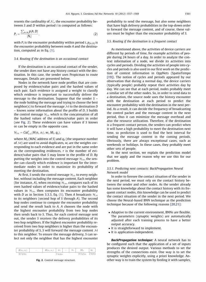
3.4. Routing if the destination is an occasional contact

If the destination is an occasional contact of the sender,the sender does not have any history contact with the des-tination. In this case, the sender uses Propicman to routemessages. Details are presented below.

Nodes in the network have node profiles that are com-posed by evidence/value pairs and the hashed values ofeach pair. Each evidence is assigned a weight to classifywhich evidence is important to successfully deliver themessage to the destination. Suppose that the sender S –the node holding the message and trying to choose the bestneighbor(s) to forward the messageM to the destination D– knows some information about the profile of D. S buildsthe control message HM which is the concatenation of allthe hashed values of the evidence/value pairs in order(see Fig. 2). These evidences can have values if S knowsor can be empty in the opposite case.

HM ¼ Catri¼1ðHðei;v iÞ;wi;MS; qSÞ;

where MS (MAC address of S) and qS (the sequence numberofM) are used to avoid duplicates, wi are the weights cor-responding to each evidence and are put in the same orderas the corresponding evidences, r is the number of evi-dence/value pairs that S may know in the profile of D. Byputting the weights into the control message HM, the sen-der can classify which evidence is important for the inter-mediate nodes in order to maximize its probability ofmeeting the destination.

At first, S sends the control message HM to every neigh-bor, without including the message content. Each neighbor(for instance, A), when receiving HM, compares each of itsown hashed values of evidence/value pairs to the hashedvalues in HM, then computes its encounter probabilitywith D as in Section 3.3.3, Eq. (1). Then A broadcasts HMto its neighbors (second hop of S through A). The secondhop nodes continue to compute the encounter probabilityand send the result back to A. A chooses the node withthe highest encounter probability from two hop nodesthen sends back to S. Thus, for each control message sentout, the sender S receives the delivery probabilities of itstwo hop neighbors. If the highest encounter probability re-ceived from two hop neighbors is higher than the encoun-ter probability of S, S will forward the message contentMto this neighbor. To ensure the message delivery, S can se-lect not only the neighbor that has the highest encounter

Fig. 2. Control message structure.

probability to send the message, but also some neighborsthat have high delivery probabilities in the top-down orderto forward the message content, and of course, these val-ues must be higher than the encounter probability of S.

3.5. Routing if the destination is a frequent contact

As mentioned above, the activities of device carriers aredifferent by periods of time, for example activities of peo-ple during 24 hours of a day. In order to analyze the con-text information of a node, we divide its activities intocycles and periods. Dividing the activities of people into cy-cles and periods is also used in our first work on the predic-tion of context information in OppNets (SpatioTempo[19]). The notion of cycles and periods appeared by ourobservation that during a normal day, the device carriers(typically people) probably repeat their activities day byday. We can see that at each period, nodes probably meeta similar set of the other nodes. So, in order to send data toa destination, the source node uses the history encounterwith the destination at each period to predict theencounter probability with the destination in the next per-iod. As a result, it can decide the frequency of broadcastingthe control packet and the message content in the nextperiod, thus it can minimize the message overhead andalso the resource utilization. Therefore, if the destinationis a frequent contact person, the senders can predict whenit will have a high probability to meet the destination nexttime, so prediction is used to find the best interval forsending the message content in the coming periods.Obviously, there are always exceptional cases, such asweekends or holidays. In these cases, they probably meetother sets of people.

In the next section, we explain the prediction modelthat we apply and the reason why we use this for ourproblem.

3.5.1. Predicting next contacts: BackPropagation NeuralNetwork model

In order to foresee the contact situation of the sender inthe next period, we must rely on the contact history be-tween the sender and other nodes. As the sender alreadyhas some knowledge about the contact history with its fre-quent contact nodes, this knowledge can be used to predictthe contact situation of the sender in the next period. Wechoose the Neural-based BNN technique as the predictiontechnique because of the following reasons [20,21]:

� Adaptive to the current environment, BNNs are flexible.The parameters (synaptic weights) are automaticallyadjusted after each training process to have a betteroutput accuracy.� It is straightforward to implement.� It is application-independent.

BackPropagation technique: A neural network has tobe configured such that the application of a set of inputsproduces the desired output. Various methods to set thestrengths of the connections exist. One way is to set thesynaptic weights explicitly, using a priori knowledge. An-other way is to train the system by feeding it with samples,

Fig. 3. A simple neural structure.

1562 H.A. Nguyen, S. Giordano / Ad Hoc Networks 10 (2012) 1557–1569

consisting of input and output values (training samples)and letting it change its synaptic weights according tosome learning rule. The first way is not suitable in our sit-uation because of lacking a priori knowledge. The Back-Propagation algorithm looks for the minimum of theerror function in the synaptic weight space using themethod of gradient descent.

The application of the training rule involves two phases:during the first phase, the input is presented and propa-gated forward through the network to compute the outputvalue for each unit. This output is then compared with thetargets, resulting in an error signal for each output unit.The second phase involves a backward pass through thenetwork during which the error signal is passed to eachunit in the network and the appropriate synaptic weightchanges are made. This second, backward pass allows forrecursive computation of output value as indicated above.The first step is to compute the error signal for each of theoutput units. This is the difference between the predictedand desired output.

When creating a functional model in CiPRO, there aresome basic components of importance. First, the inputs ofthe neuron are modeled as synaptic weights. The strengthof the connection between an input and a neuron is notedby the value of the synaptic weight. The next two compo-nents model the actual activity within the neuron. An addersums up all the inputs modified by their respective synapticweights. Finally, an activation function controls the ampli-tude of the output (usually between 0 and 1).

3.5.2. Using BackPropagation model to predict the encounterprobability with the destination within the next period

In order to predict the contact situation of a device car-rier in the next period, we rely on two input parameters:the history encounter of the device carrier in the currentperiod (the horizontal input) and the history encounterof the carrier in the same periods as the next period ofthe previous cycles (the vertical input). Whenever the nodehas a message to send to a frequent contact, it will com-pute the encounter probability with the destination at eachperiod. These values are stored at the node for the predic-tion in the next cycles. The history encounter (encounterprobability) between the node and the frequent contactsis computed cumulatively at the same period as the previ-ous cycles in the past as in Eq. (3).

The prediction happens at each period, the output valueis then compared with the actual value and changes maybe applied to have better prediction function in the nextperiod, such that the predicted result must be as close tothe actual result as possible.

3.5.2.1. Predict the output value. Let us look at Fig. 4 wherePi

j (j 2 [1, . . . ,K]), (i 2 [1, . . . ,C]) is the encounter probabilitywith the destination within the period i in cycle j, definedin Section 3.3.3. K is the number of previous cycles in thepast that we take into account to create the vertical input,C is the number of periods in each cycle. Suppose that weare in period (i � 1) of the current cycle (cycle 0); the con-text situation in this period is denoted by P0

i�1. We want topredict the context situation ðP0

i Þ in the next period (periodi, cycle 0).

For the sake of simplicity, which is important for re-source-constrained devices, in the implementation wecumulate the encounter probabilities Pj

i (j 2 [1, . . ., ,K]) tocompute the vertical input at the period i as in Eq. (3). Asa result, after each cycle, the node contains only the latestcontext value of each period.

Pc1i ¼

P1i þ Pc2

i

2; ð3Þ

where Pc2i is the cumulative value at period i of cycle 2, Pc1

i

is the cumulative value at period i of cycle 1.In order to predict the encounter probability with the

destination in the next period i, we build a simple formof a neural network with BackPropagation algorithm asFig. 5. In the figure, the horizontal input, denoted by Ih isthe current encounter probability, thus Ih ¼ P0

i�1; the verti-cal input, denoted by Iv, is the cumulative values ofPj

iðj 2 ½1; . . . ; ;K�Þ, thus Iv ¼ Pc1i and is computed as in Eq.

(3). The corresponding synaptic weights of the verticaland horizontal inputs (the synaptic weights in Fig. 3) arewv, wh respectively.

� The summing junction function:

m ¼ Ivwv þ Ihwh; ð4Þ

� The normalization function: As mentioned previously,the activation function acts as a normalization function,such that the output of the neuron is between certainvalues (0 and 1, in our case).

U ¼ mwv þwh

¼ Ivwv þ Ihwh

wv þwh: ð5Þ

The output of the activation function is the predictedencounter probability with the destination within the nextperiod. Therefore, the predicted encounter probability Ppred

of the next period is as follows:

Ppred ¼Ivwv þ Ihwh

wv þwh: ð6Þ

3.5.2.2. Error function. In Neural Network, this function isalso called Mean Squared Error (MSE) between the actualoutput and the desired output (in our case, it is predicted

Fig. 4. Vertical and horizontal parameters.

Fig. 5. Prediction process with BackPropagation Neural Network model.

H.A. Nguyen, S. Giordano / Ad Hoc Networks 10 (2012) 1557–1569 1563

output) for a given input in the training example (one per-iod). This is simply the average of the squares of the differ-ence between what we predict and what we got. Thus, ourerror function can be formally written as:

E ¼ ðPpred � PactualÞ2

2; ð7Þ

where Ppred is the predicted value and Pactual is the actualvalue of the period.

3.5.3. Routing processBased on the predicted information, senders will have a

suitable decision on the number of broadcasts of the mes-sage in this period. They can increase the number of broad-casts in the period that has high encounter probabilitywith the destination or they will not initiate the routingprocess in the period that has very low rate. The definitionof the encounter probability within a period is presented inEq. (2) and how to predict it in Section 3.5.2, Eq. (6).

CiPRO concentrates on the spatial and temporal aspectsof the devices. The sender uses the predicted encounterprobability within the next period to decide how manytimes to resend the message header in order to have thehighest encounter probability with the destination withoutflooding the network.

Assume that we are currently in the period (i � 1), we

already knew the encounter probability P0i�1

� �within this

period, we want to predict P0i of the next period i.

The sender S uses two input parameters to predict P0i :

the horizontal input P0i�1, denoted by Ih and the vertical in-

put, denoted by Iv, which is the cumulative encounterprobability of the same periods as i of the previous cycles

Pji; j 2 ½1::K�

� �. To avoid containing too much data at the

sender, we use the vertical input as the cumulativeencounter probability as shown in Eq. (3).

At the beginning, S can be in one of the two states asfollows:

1. S has not yet passed any previous cycles yet (initialstate), there is not a vertical input for the neural net-work. We set this value equal to 0; the initial horizontalsynaptic weight is 0.5. Thus the predicted value is com-puted as follows:

Ppred ¼Ivwv þ Ihwh

wv þwh¼ Ih:

The synaptic weight adjustment as computed in Eq.(A.3) for the next prediction is:

Dwh ¼ cbiIh ¼ cðPpred � PactualÞ1

wv þwhIh

¼ cðPpred � PactualÞ1

whIh ¼ 2cIhðIh � PactualÞ; ð8Þ

2. S has passed some previous cycles (in most of thecases), we apply the computation for the prediction asin Eq. (5):

Ppred ¼m

wv þwh¼ Ivwv þ Ihwh

wv þwh:

After each period, the vertical and horizontal synapticweights are adjusted as follows:

wv ¼ wv�old þ Dwv with Dwv ¼ cbiIv ;

wh ¼ wh�old þ Dwh with Dwh ¼ cbiIh;

where bi ¼ ðPpred � PactualÞ 1wvþwh

.

Finally, after each prediction, changes can be made tothe synaptic weights of the vertical and horizontal inputsof the next prediction. Once the sender has the expected

0.2

0.4

0.6

0.8

1

Nor

mal

ized

Erro

r

"percentError.data"

1564 H.A. Nguyen, S. Giordano / Ad Hoc Networks 10 (2012) 1557–1569

encounter probability within the next period, it will decideon the number of broadcasts of the message header in thenext period.

Given u the maximum broadcast capacity of S in theperiod i, the number of broadcasts of the message headerin the period i will be a rounded value as follows:

y ¼ b/Ppredc; 0 < / 6 u: ð9Þ

In Eq. (9), the parameter / is flexible, depends on the con-straints of nodes to the system. In other words, if the mes-sage is important, and the network overhead is not aproblem, in this case, the communication delay is animportant parameter, the parameter / is set to maximum(equal to u). Thus, after the prediction process, if the pre-dicted encounter probability within the next period is high,the sender must increase the number of broadcasts of themessage header to maximize the capacity of sending themessage to the intermediate nodes that have the highencounter probability with the destination in the future.

Assuming U is the number of units of time in a period,for the next period, the sender will broadcast the messageheader in every bUyc ¼ b U

/Ppredc units. By predicting the con-

text information in the next period, the sender can adap-tively have a suitable routing strategy by deciding thefrequency of broadcasting the message headers in the nextperiod.

4. Simulation results and performance evaluation

4.1. Mobility model and simulation description

The simulation scenario is a rectangle of 1870 �1520 m, divided in a 2 � 6 grid. We simulate 50 nodes,with the transmission range of 30 m. The mobility modelused in the simulation is the Community-based MobilityModel [22]. Its main idea is to model nodal mobility basedon human social relationships and thus identify communi-ties. The communities are then placed into the celled net-work area, and each community occupies a cell. A nodemoves randomly in its cell. When it is outside of its cell,its moving decisions depend on the social attractiveness(importance in terms of the social relationships). Wedeveloped the simulator in Java based on the traces gener-ated from CMM model.1

The simulation is executed based on some assumptions:The nodes have unlimited power, no constraint about thestorage space, neither the memory space, if a node trans-mits a message to another node, the message will be re-ceived correctly (no data loss).

In our simulation, nodes move according to the tracesgenerated by this model, where we map the social commu-nity notion with the grid in the simulation scenario and thesocial attractiveness of a community (grid) to a node is thetime during a day the node stays in this grid. The simulatedduration is 14 cycles, one cycle corresponds to one day, andperiods to hours. The routing algorithm is evaluated untilthe first copy of the message reached the destination. The

1 The simulation source code is available on http://www.people.usi.ch/nguyenh/, the movement traces generator is available on http://www.cs.st-andrews.ac.uk/mirco/software.html

weekend days are considered exceptions (behavior is dif-ferent from the other days of the week).

At the beginning, each node randomly has 8 frequentdestinations. For the training process, both the verticaland horizontal synaptic weights are 0.5, as well as thelearning rate. During the simulation, the messages weresent out from arbitrary senders, 75% of them were sentto the frequent destinations of the sources. The simulationresults are the average results from 16 simulation runswith the 95% confidence level.

At period i, if node S has messageM to send to destina-tion D, there are two cases:

1. D is one of the frequent contacts of S, S will predict theencounter probability within the next period (i + 1).

2. D is not a frequent contact of S. In this case, S uses Pro-picman to route the message.

Note that when there is a message to send to a destina-tion, this message can go through some intermediatenodes. Then each node uses its relationship with the desti-nation to decide which routing technique will be em-ployed: CiPRO in the case that the destination is one ofits frequent destinations, or Propicman in the oppositecase.

4.2. Evaluation of the contact prediction

Fig. 6 shows the percent error of the prediction. Asshown in the figure, the precision increases by cycles andperiods. During the first cycles (cycles 1–4), the node doesnot have enough context information to predict theencounter probability within the next period, and as a re-sult, the predicted value and the desired value are very dif-ferent. Thanks to the learning process with synaptic weightadjustments and the impact of the learning rate after eachperiod, in time, period by period, cycle by cycle, these twovalues come closer. This tendency is represented by thedecrement of the percent error shown in Fig. 6. Of course,there are still some points that have quite big relative per-centage value (cycle 9, for instance), this happens for theexceptional cases. From cycle 4 onward, the percent errorindex goes down, from around 20% down to around 7%. It

01 2 3 4 5 6 7 8 9 10 11 12 13

Cycles

Fig. 6. Percent Error of the prediction. Each cycle is one day.

H.A. Nguyen, S. Giordano / Ad Hoc Networks 10 (2012) 1557–1569 1565

is the result of the learning process, through periods toperiods, with the experience achieved after each learningprocess, the synaptic weights are adjusted to have the pre-dicted outputs as close as possible to the desired values.Thus, after some cycles (cycle 5), the predicted result be-comes more stable. The percent error goes down around7%. This is an acceptable level if we consider the typicalcharacteristics of OppNets.

4.3. Impact factors and performance evaluation

In the performance evaluation, we compared CiPROwith three representative routing protocols (context-obliv-ious, mobility-based and social context-based routing pro-tocols as mentioned in Section 2): Epidemic, ProPHET andPropicman respectively. We ran all these routing solutionsin the same testbed with the same scenario to evaluatetheir performance. We have focused on comparing theirperformance with regard to the following metrics. First ofall, we are interested in the network overhead: how manyadditional bytes are sent for successfully delivering a mes-sage to a destination. Applications using OppNets shouldbe relatively delay tolerant, but it is still of interest to con-sider the message delivery delay to know how long it takesa message to be delivered.

Moreover, we vary the number of nodes and their selec-tion for routing to see the impact on the performance ofthe node density and of the number of selected candidatesat each neighbor selection. As in the simulation scenario,the speed of nodes and the sending rate are randomly gen-erated, we do not consider their impact on the perfor-mance. During the evaluation, sometime we use the term‘‘routing process’’. A routing process is started when a nodebroadcast the control packet and is ended by finding thenext hop forwarder.

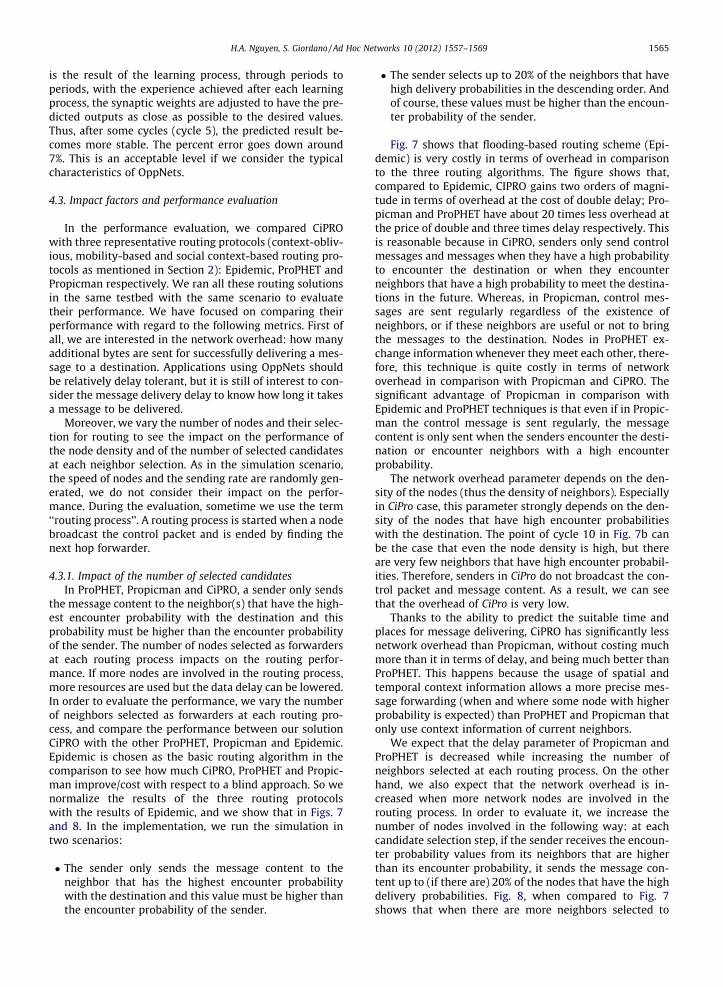
4.3.1. Impact of the number of selected candidatesIn ProPHET, Propicman and CiPRO, a sender only sends

the message content to the neighbor(s) that have the high-est encounter probability with the destination and thisprobability must be higher than the encounter probabilityof the sender. The number of nodes selected as forwardersat each routing process impacts on the routing perfor-mance. If more nodes are involved in the routing process,more resources are used but the data delay can be lowered.In order to evaluate the performance, we vary the numberof neighbors selected as forwarders at each routing pro-cess, and compare the performance between our solutionCiPRO with the other ProPHET, Propicman and Epidemic.Epidemic is chosen as the basic routing algorithm in thecomparison to see how much CiPRO, ProPHET and Propic-man improve/cost with respect to a blind approach. So wenormalize the results of the three routing protocolswith the results of Epidemic, and we show that in Figs. 7and 8. In the implementation, we run the simulation intwo scenarios:

� The sender only sends the message content to theneighbor that has the highest encounter probabilitywith the destination and this value must be higher thanthe encounter probability of the sender.

� The sender selects up to 20% of the neighbors that havehigh delivery probabilities in the descending order. Andof course, these values must be higher than the encoun-ter probability of the sender.

Fig. 7 shows that flooding-based routing scheme (Epi-demic) is very costly in terms of overhead in comparisonto the three routing algorithms. The figure shows that,compared to Epidemic, CIPRO gains two orders of magni-tude in terms of overhead at the cost of double delay; Pro-picman and ProPHET have about 20 times less overhead atthe price of double and three times delay respectively. Thisis reasonable because in CiPRO, senders only send controlmessages and messages when they have a high probabilityto encounter the destination or when they encounterneighbors that have a high probability to meet the destina-tions in the future. Whereas, in Propicman, control mes-sages are sent regularly regardless of the existence ofneighbors, or if these neighbors are useful or not to bringthe messages to the destination. Nodes in ProPHET ex-change information whenever they meet each other, there-fore, this technique is quite costly in terms of networkoverhead in comparison with Propicman and CiPRO. Thesignificant advantage of Propicman in comparison withEpidemic and ProPHET techniques is that even if in Propic-man the control message is sent regularly, the messagecontent is only sent when the senders encounter the desti-nation or encounter neighbors with a high encounterprobability.

The network overhead parameter depends on the den-sity of the nodes (thus the density of neighbors). Especiallyin CiPro case, this parameter strongly depends on the den-sity of the nodes that have high encounter probabilitieswith the destination. The point of cycle 10 in Fig. 7b canbe the case that even the node density is high, but thereare very few neighbors that have high encounter probabil-ities. Therefore, senders in CiPro do not broadcast the con-trol packet and message content. As a result, we can seethat the overhead of CiPro is very low.

Thanks to the ability to predict the suitable time andplaces for message delivering, CiPRO has significantly lessnetwork overhead than Propicman, without costing muchmore than it in terms of delay, and being much better thanProPHET. This happens because the usage of spatial andtemporal context information allows a more precise mes-sage forwarding (when and where some node with higherprobability is expected) than ProPHET and Propicman thatonly use context information of current neighbors.

We expect that the delay parameter of Propicman andProPHET is decreased while increasing the number ofneighbors selected at each routing process. On the otherhand, we also expect that the network overhead is in-creased when more network nodes are involved in therouting process. In order to evaluate it, we increase thenumber of nodes involved in the following way: at eachcandidate selection step, if the sender receives the encoun-ter probability values from its neighbors that are higherthan its encounter probability, it sends the message con-tent up to (if there are) 20% of the nodes that have the highdelivery probabilities. Fig. 8, when compared to Fig. 7shows that when there are more neighbors selected to

Messages0 5 10 15 20 25

seco

nds

0

500

1000

1500

2000

2500Transmission delay

PropicmanProPhetEpidemicCiPro

Messages0 5 10 15 20 25

Nor

mal

ized

net

wor

k ov

erhe

ad

2.0

3.0

4.0

5.0

6.0Normalized network overhead (Logarithmic scale)

PropicmanProPhetEpidemicCiPro

Fig. 7. (a and b) show the delay and the overhead of CiPRO, Propicman, Prophet compared to Epidemic when only the neighbor with the highest encounterprobability is selected. Figure (b) shows the semi-logarithmic plot of overhead comparison. In (b), the overhead caused by CiPRO is around two orders ofmagnitude less than Epidemic at the cost of double delay (a), whereas (a) shows that CiPRO has around 2 times. Propicman and ProPHET have about 20times less overhead at the price of double and three times delay respectively. CiPRO has the best performance in term of network overhead (confidencelevel=95%).

Messages0 5 10 15 20 25

seco

nds

0

200

400

600

800

1000

1200Transmission delay

PropicmanProPhetEpidemicCiPro

Messages0 5 10 15 20 25

Nor

mal

ized

net

wor

k ov

erhe

ad

3.0

4.0

5.0

6.0Normalized network overhead (Logarithmic scale)

PropicmanProPhetEpidemicCiPro

Fig. 8. (a and b) show the delay and the overhead of CiPRO, Propicman, Prophet compared to Epidemic when only the neighbor with the highest encounterprobability is selected. Fig. 7b shows the semi-logarithmic plot of overhead comparison. In (b), the overhead caused by CiPRO is around two orders ofmagnitude less than Epidemic at the cost of double delay (a), whereas (a) shows that CiPRO has around 2 times. Propicman and ProPHET have about 20times less overhead at the price of double and three times delay respectively. CiPRO has the best performance in term of network overhead (confidencelevel=95%).

1566 H.A. Nguyen, S. Giordano / Ad Hoc Networks 10 (2012) 1557–1569

send the message content at each routing process, delay isreduced at the price of higher overhead. However, as thegain in terms of delay is not high, we can conclude thatthere is no evident advantage in selecting more than oneneighbor (assuming no losses). Clearly, if we release theassumption that no message is lost, the problem changes,and this is matter of ongoing work.

4.3.2. Impact of the node densityWe investigate the scalability of the routing algorithms

by increasing the number of nodes from 50 up to 250nodes in steps of 50.

In Propicman, senders regularly broadcast the controlmessage to find the best forwarder(s). Only the neighborthat has the highest encounter probability will be selected

by the sender to forward the message content. Thus, thereis no significant change in terms of overhead as each time,only the neighbor with the highest encounter probability isselected (in other words, the maximum number of neigh-bors that will receive the message is fixed by the protocol).We can only appreciate some improvement in terms of de-lay as we increase the probability of finding a better for-warder as we increase the population. Similar reasoningapplies to CIPRO, where the overhead also remains quitestable, and we observe some improvements in terms of de-lay (Fig. 9).

On the contrary, if we increase the node density, thereare more nodes involved, messages in the flooding-basedrouting scheme will quickly invade the entire network.As a result, the message will reach the destination more

0

1

2

3

4

5

6

7

8

50 100 150 200 250

Nor

mal

ized

del

ay

Number of Nodes

Delay with different node densities

EpidemicProPHET

PropicmanCiPRO

0

0.05

0.1

1

50 100 150 200 250

Nor

mal

ized

net

wor

k ov

erhe

ad

Number of Nodes

Overhead with different numbers of nodes

EpidemicProPHET

PropicmanCiPRO

Fig. 9. (a and b) show the delay and the overhead of CiPRO, Propicman, Prophet and Epidemic in the case of varying the number of nodes. The delay andoverhead of Epidemic are normalized to 1 and the other algorithms are normalized by the Epidemic curves. With more nodes involved, the delay caused byEpidemic is dramatically decreased, whereas the delays caused by ProPHET, Propicman and CiPRO are slightly decreased. The network overhead caused byEpidemic is much increased, the overhead caused by ProPHET is slightly increased. The overhead caused by CiPRO and ProPHET shows to be less dependenton the number of nodes (confidence level=88%).

H.A. Nguyen, S. Giordano / Ad Hoc Networks 10 (2012) 1557–1569 1567

quickly (Fig. 9a), thus the message delay is decreased.However, because of the flooding of messages on the net-work, this routing technique is very costly in terms of net-work overhead in comparison with the other techniques asshown in Fig. 9b. Increasing the number of nodes is alsoimportant in ProPHET, if we increase the number of nodes,the number of contacts that a node may have will increase.As a consequence, there are more control packets ex-changed, thus more overhead uploaded to the network.

To conclude, if we increase the node density, the mes-sage delay is much improved in the case of Epidemic,slightly improved in the case of ProPHET, Propicman andCiPRO as there may be more nodes with high deliveryprobabilities. However, Epidemic is very costly in termsof network overhead, this parameter is slightly increasedin the case of ProPHET as there are more control packetsexchanged between nodes. In the case of Propicman andCiPRO, increasing the node density does not significantlyimpact the performance of the algorithms.

5. Conclusion and future work

We applied the BackPropagation Neural Network modelto predict the behavior of device carriers. The evaluationanalysis and the simulation results indicate that for thecontext-based routing algorithms in OppNets, CiPRO –the BNN-based solution – outperforms other routing solu-tions thanks to its ability to maximize the delivery ratioand to minimize the network overhead.

This work is the first contribution to date that employsthe BNN model to predict the mobility pattern in OppNets.In our future work, we will continue to evaluate the perfor-mance of CiPRO by evaluating the impact of the number offrequent contacts to the CiPRO performance. Especially, inorder to better evaluate our social context-based routingtechniques, currently we are doing a real experiment tocapture the real social contact with the participants wear-ing sensor nodes (Telosb). The collected traces will be thefirst case of contact traces with context information.

The other interesting work is to investigate the possibil-ity of leveraging long term repetitive patterns in thebehavior of nodes to minimize the overhead of the learningprocess and therefore the computational cost.

Acknowledgments

We would like to thank Prof. Luca Maria Gambardella(IDSIA-Istituto Dalle Molle di Studi sull’Intelligenza Artifi-ciale) for his valuable suggestions in prediction with Neu-ral Networks. We also would like to thank the reviewersfor their insightful comments on the paper.

Appendix A. Training data with BNN model: synapticweights, learning rate adjustments

For any given training sequence, this value is a functionof the synaptic weights of the network. So, to reduce theerror, it is necessary to control the gradient of the errorfunction with respect to each synaptic weight. One maythen move each synaptic weight slightly in the oppositedirection to the gradient. The gradient is defined as thevector of partial derivatives of the multivariate functionwith respect to each variable. Because the error functionis a function of the network output, we first need tocalculate the partial derivative of the network outputwith respect to each associated connection weight.Since all other variables but the one of interest are heldconstant when we calculate the partial derivative, onlyone linear term is left in the calculation of the partial deriv-ative of the output, and leaving the coefficient - which isjust the corresponding input. So we compute the synapticweight adjustment of the vertical and horizontal inputsas follows:

The synaptic weight of the vertical input – wv:

dEdwv

¼ dEdPpred

dPpred

dmdm

dwv: ðA:1Þ

From Eqs. 4, 5, 7, we have:

1568 H.A. Nguyen, S. Giordano / Ad Hoc Networks 10 (2012) 1557–1569

dEdPpred

¼ Ppred � Pactual;dPpred

dm¼ 1

wv þwh;

dmdwv

¼ dðIvwv þ IhwhÞdwv

¼ Iv :

Eq. (A.1) becomes:

dEdwv

¼ ðPpred � PactualÞ1

wv þwhIv :

Let bi ¼ ðPpred � PactualÞ 1wvþwh

- this is the proportionalamount of the product of the error signal. We have the syn-aptic weight adjustment of the vertical input:

Dwv ¼ gvbiIv : ðA:2Þ

We do the same for the horizontal input and have the syn-aptic weight adjustment:

Dwh ¼ ghbiIh; ðA:3Þ

where g is the learning rate. The learning procedure re-quires that the change of synaptic weights is proportionalto dE

dw. The constant of proportional is the learning rate.When the learning rate is low, small steps are taken inthe gradient direction; when the learning rate is high, largesteps are taken. For practical purposes, we choose a learn-ing rate that is as large as possible without leading to oscil-lation. The pseudo-Newton method [23] proposed theadaptive learning rates as follows:

gv ¼1

d2Ed2wv

������þ 1

; gh ¼1

d2Ed2wh

������þ 1

:

In the pseudo-Newton case, the learning rate is low whenthe absolute value of the second order derivative is highand vice versa. That is, if the error surface has high curva-ture – corresponding to large changes in the gradient oversmall intervals – the step size is small to avoid catastrophicsteps in the wrong direction.

References

[1] H. Nguyen, S. Giordano, A.Puiatti, Probabilistic routing protocol forintermittently connected mobile ad hoc networks (PROPICMAN), in:IEEE WoWMoM/AOC 2007, Helsinki, 2007.

[2] M. Musolesi, S. Hailes, C. Mascolo, Adaptive routing forintermittently connected mobile ad hoc networks, in: The 6thInternational Symposium on a World of Wireless, Mobile, andMultimedia Networks (WoWMoM), Taormina, Giardini Naxos,June, 2005.

[3] H. Nguyen, S. Giordano, Routing in opportunistic networks,International Journal of Ambient Computing and Intelligence(IJACI) 1.

[4] M. Conti, J. Crowcroft, S. Giordano, P. Hui, H.A. Nguyen, A. Passarella,MiNEMA: Middleware for Network Eccentric and MobileApplications, Springer, Berlin, Heidelberg, New York, USA, 2009.

[5] A. Vahdat, D. Becker, Epidemic Routing for Partially-Connected AdHoc Networks, Tech. Rep., 2000.

[6] J. Widmer, J.L. Boudec, Network coding for efficient communicationin extreme networks, in: ACM SIGCOMM 2005, Workshop on DelayTolerant Networking (WDTN), Philadelphia, 2005.

[7] M. Grossglauser, N. David, Mobility increases the capacity of ad hocwireless networks, IEEE/ACM Transactions on Networking 10.

[8] A. Lindgren, A. Doria, O. Schelen, Probabilistic routing inintermittently connected networks, ACM SIGMOBILE MobileComputing and Communications Review 7.

[9] P. Hui, J. Crowcroft, E. Yoneki, Bubble rap: social-based forwarding indelay tolerant networks, in: The 9th ACM Int. Symposium on MobileAd Hoc Networking and Computing (MobiHoc), 2008.

[10] C. Mascolo, M. Musolesi, SCAR: context-aware adaptive routing indelay tolerant mobile sensor networks, in: IWCMC ’06: Proceedingsof the 2006 International Conference on Wireless Communicationsand Mobile Computing, ACM, New York, USA, 2006, pp. 533–538.

[11] B. Burns, O. Brock, B.N. Levine, MV routing and capacity building indisruption tolerant networks, in: IEEE INFOCOM 2005, Miami, FL,March, 2005.

[12] J. Burgess, B. Gallagher, D. Jensen, B.N. Levine, Maxprop: routing forvehicle-based disruption-tolerant networking, in: IEEE INFOCOM,Barcelona, April, 2006.

[13] J. Leguay, A. Lindgren, J. Scott, T. Friedman, J. Crowcroft,Opportunistic content distribution in an urban setting, in: 2006SIGCOMM Workshop on Challenged Networks (CHANTS 2006), Pisa,Italy, September, 2006.

[14] C. Boldrini, M. Conti, I. Jacopini, A. Passarella, HiBOp: a history basedrouting protocol for opportunistic networks, in: WoWMoM 2007,Helsinki, June, 2007.

[15] J. Ghosh, S.J. Philip, C. Qiao, Sociological Orbit Aware LocationApproximation and Routing (SOLAR) in MANET, ELSEVIER Ad HocNetworks 5.

[16] E. Nathan, A. Pentland, Reality mining: sensing complex socialsystems, Personal and Ubiquitous Computing 10 (2006) 255–268.ISSN 1617-4909.

[17] D.O. Olguin, P.A. Gloor, A.S. Pentland, Capturing individual and groupbehavior with wearable sensors, in: AAAI Spring Symposium onHuman Behavior Modeling, 2009.

[18] A. Madan, Y. Pentland, Modeling social diffusion phenomena usingreality mining, in: AAAI Spring Symposium on Human BehaviorModeling, 2009.

[19] H. Nguyen, S. Giordano, Spatiotemporal routing algorithm inopportunistic networks, in: IEEE WoWMoM/AOC, California, June,2008.

[20] T.W.S. Chow, S.-Y. Cho, Neural Networks and Computing: LearningAlgorithms and Applications, Imperial College Press, 57 SheltonStreet, Convent Garden, London, 2007.

[21] D.P. Mandic, J.A. Chambers, Recurrent Neural Networks ForPrediction: Learning Algorithms Architectures and Stability, Wiley,Baffins Lane, Chichester, W. Sussex, England, 2001.

[22] M. Musolesi, C. Mascolo, A community based mobility model for adhoc network research, in: ACM/SIGMOBILE REALMAN, Florence,Italy, May, 2006.

[23] L. Ricotti, S. Ragazzini, G. Martinelli, Learning of word stress in a sub-optimal second order back-propagation neural network, NeuralNetworks 1.

Hoang Anh Nguyen is a Ph.D candidate at theNetworking Labs, Information System andNetworking Institute (ISIN), University ofApplied Sciences (SUPSI), Switzerland. Heholds an M.Sc degree in Computer Sciencefrom Institute National Polytechnique deToulouse (INPT), France. Actually, he isworking on context-based routing protocolsin opportunistic networks.

Silvia Giordano holds a Ph.D from EPFL,Switzerland. She is currently the head of theNetworking Lab (NetLab) in the Institute ofSystem for Informatics and Networking (ISIN),and as direction member of ISIN, at the Uni-versity of Applied Science – SUPSI in Ticino,Switzerland. She is teaching several courses inthe areas of: Networking, Wireless and MobileNetworking, Quality of Services and NetworksApplications.She is co-editor of the book ’’Mobile Ad HocNetworking’’ (IEEE-Wiley 2004). She has

published extensively on journals, magazines and conferences in theareas of quality of services, traffic control, wireless and mobile ad hocnetworks. She has participated in several European ACTS/IST projects and

H.A. Nguyen, S. Giordano / Ad Hoc Networks 10 (2012) 1557–1569 1569

European Science Foundation (ESF) activities. Since 1999 she serves asTechnical Editor of IEEE Communications Magazine, and is currentlyeditor of the series co-editor of the new Series on Ad Hoc And SensorNetworks of the IEEE Communication Magazine. She is also editor of Adhoc networks journal by Elsevier, Ad Hoc & Sensor Wireless Networksjournal, Ocpscience, Journal of Ubiquitous Computing and Intelligence(JUCI) and Journal of Autonomic and Trusted Computing (JoATC) both byAmerican Scientific Publishers (ASP), and Mediterranean Journal ofComputer and Networks, SoftMotor. She was already co-editor of severalspecial issues of IEEE Communications Magazine and Baltzer MONET andCluster Computing on mobile ad hoc networking and QoS networking.

She will be general chair of WoWMoM 2009, program co-chair of IEEEPERCOM 2009, was program co-chair of IEEE VTC-Fall 2008, IEEE MASS2007, workshop chair of IEEE WOWMoM 2007, tutorial chair of MobiHoc2006, general chair of IEEE WONS 2005, organizer of IEEE Persens 2005–2009 workshop, IEEE AOC2005–2009 workshop and ACM Mobihoc SANETworkshop 2007–2008 and is/was on the executive committee and TCP ofseveral international conferences, and serves as reviewer on transactionsand journals, as well as for several important conferences. Prof. SilviaGiordano is a member of IEEE Computer Society, ACM and IFIP WG 6.8.Her current research interests include wireless and mobile ad hoc net-works, QoS and traffic control.