Context dependent compression using Adaptive Subsampling of

Scientific Datasets

T A L L A T M A H M O O D S H A F A A T

Master of Science Thesis Stockholm, Sweden 2006

ICT/ECS-2006-12

Abstract

Numerical simulations employed by researchers generate large data sets; data sets that on

one hand consume terabytes of storage and on the other, out-strip the ability to

manipulate, visualize and analyze it. A challenge in large scale computing is to reduce

these enormous data sets without loosing critical information, and finding ways to apply

numerical techniques directly to the compressed data. Based on these data sets, we

present a comparison of two subsampling based algorithms, Fixed Interval Subsampling

and Adaptive Coarsening. Fixed Interval Subsampling divides the data set into blocks of

predefined size, while Adaptive Coarsening produces a multiresolution, hierarchical

representation, dividing the original data into unequal partitions. We achieved

compression of 19 for one dimensional data, and 17 for two dimensional. From the

results of the comparison of the two methods, we choose the better technique and use it to

show that numerical analysis techniques like the finite difference method can be applied

directly to the reduced data set with satisfactory tolerance and note able compression,

thus requiring less compute and storage resources. We also present results that

demonstrate that it is important to know the context in which the data will be used before

compressing it, thus enabling us to provide guaranteed error bounds on the post

manipulations.

Acknowledgements

This thesis work has been carried out at the Department of Microelectronics and

Information Technology, Royal Institute of Technology (KTH) Sweden. First and

foremost, I would like to thank my advisor Prof. Scott B. Baden, University of California

at San Diego (UCSD) for permitting me to carry out this project under his supervision. I

am grateful for his support, encouragement and guidance; this work would not have been

possible without his insight and advice and I enjoyed a lot working with him.

I also wish to thank my examiner Prof. Mihhail Matskin, Royal Institute of Technology

(KTH) for giving valuable feedback, helping arranging for computer access and

reviewing my report.

Special thanks to my friends for their assistance at the various stages of this work and

also for making my stay at KTH, Sweden memorable.

Finally, I dedicate this work to my parents, my sisters and brother. Words alone cannot

express the gratitude I owe to them for their unlimited encouragement, love and support.

To my parents

Table of contents ABSTRACT .................................................................................................................................................. 2 ACKNOWLEDGEMENTS ......................................................................................................................... 3 TABLE OF CONTENTS ............................................................................................................................. 5 LIST OF FIGURES...................................................................................................................................... 6 LIST OF TABLES........................................................................................................................................ 6 1 INTRODUCTION............................................................................................................................... 7 2 BACKGROUND ............................................................................................................................... 10

2.1 SCIENTIFIC DATASETS................................................................................................................ 10 2.2 LOSSY AND LOSSLESS COMPRESSION TECHNIQUES .................................................................... 13 2.3 TEMPORAL VS. SPATIAL COMPRESSION ..................................................................................... 13 2.4 DIGITAL FILTER BANKS AND THE WAVELET TRANSFORM.......................................................... 13 2.5 INTERPOLATION FOR REFINING................................................................................................... 15

2.5.1 Linear interpolation.............................................................................................................. 15 2.5.2 Lagrange Interpolation......................................................................................................... 15 2.5.3 Piecewise cubic hermite interpolating polynomial............................................................... 16

2.6 TAYLOR SERIES.......................................................................................................................... 18 2.7 FINITE DIFFERENCE.................................................................................................................... 18

2.7.1 Finite difference on regular grids using Taylor Series......................................................... 19 2.7.2 Finite difference on irregular grids ...................................................................................... 20

2.8 RELATED WORK ......................................................................................................................... 23 3 METHOD & IMPLEMENTATION............................................................................................... 24

3.1 SUB SAMPLING........................................................................................................................... 24 3.1.1 Fixed Interval algorithm....................................................................................................... 25 3.1.2 Adaptive Coarsening algorithm............................................................................................ 28

3.2 FINITE DIFFERENCE.................................................................................................................... 30 3.2.1 OD ........................................................................................................................................ 31 3.2.2 OCDR ................................................................................................................................... 32 3.2.3 ODCR ................................................................................................................................... 32 3.2.4 OCRD ................................................................................................................................... 33

3.3 SUB SAMPLING ON TWO DIMENSIONAL DATA............................................................................. 34 4 ANALYSIS ........................................................................................................................................ 39

4.1 DIFFERENT INTERVAL SIZES USING FI ........................................................................................ 40 4.2 COMPARISON OF USING PCHIP AND LINEAR INTERPOLATION ...................................................... 41 4.3 FI VS AC .................................................................................................................................... 42 4.4 CONTEXT DEPENDENT COMPRESSION......................................................................................... 43

4.4.1 ODCR ................................................................................................................................... 43 4.4.2 OCDR ................................................................................................................................... 44 4.4.3 OCRD ................................................................................................................................... 45 4.4.4 Comparison .......................................................................................................................... 46

4.5 COMPRESSION IN 2D .................................................................................................................. 47 5 CONCLUSIONS AND FUTURE WORK ...................................................................................... 49 6 APPENDIX........................................................................................................................................ 50

6.1 PSEUDOCODE FOR OCDR........................................................................................................... 50 6.2 READINGS .................................................................................................................................. 52

7 REFERENCES.................................................................................................................................. 53

List of Figures FIGURE 2.1 SNAPSHOTS OF THE 1D DATASET AT T=0,0.6,1.3 AND 2 ................................................................ 11 FIGURE 2.2 SNAPSHOT OF 2D DATA................................................................................................................. 12 FIGURE 2.3 FILTER BANKS AND WAVELETS ..................................................................................................... 14 FIGURE 2.4 COMPARISON OF LINEAR AND CUBIC HERMITE PIECEWISE INTERPOLATION .................................. 18 FIGURE 2.5 UNIFORM AND NON-UNIFORM SAMPLED POINTS ........................................................................... 20 FIGURE 3.1 SUBSAMPLING IN (A) ONE DIMENSION (B) TWO DIMENSION............................................................. 24 FIGURE 3.2 FIXED INTERVAL ALGORITHM ....................................................................................................... 25 FIGURE 3.3 PSEUDO CODE FOR THE FIXED INTERVAL ALGORITHM .................................................................. 27 FIGURE 3.4 ADAPTIVE COARSENING ALGORITHM ............................................................................................ 28 FIGURE 3.5 PSEUDO CODE FOR THE ADAPTIVE COARSENING ALGORITHM ....................................................... 29 FIGURE 3.6 INTERPOLATING FOR TAKING DERIVATIVE ..................................................................................... 34 FIGURE 3.7 BLOCK DISTRIBUTION................................................................................................................... 35 FIGURE 3.8 BUNCOARSENED .......................................................................................................................... 35 FIGURE 3.9 MARKED BUNCOARSENED ............................................................................................................ 36 FIGURE 3.10 2D VIEW OF BLOCKS 103-110 ..................................................................................................... 37 FIGURE 3.11 BLOCKS 103-110 CONCATENATED IN THE X-DIR ......................................................................... 37 FIGURE 3.12 BLOCKS 103-110 CONCATENATED IN THE X-DIR ......................................................................... 38 FIGURE 4.1 COMPRESSION USING DIFFERENT INTERVAL SIZES IN FI ................................................................. 40 FIGURE 4.2 LINEAR VS. PCHIP INTERPOLATION USING AC ............................................................................... 41 FIGURE 4.3 FI VS AC (A)10-3 (B)10-4 (C)10-5 (D)COMPARISON ..................................................................... 42 FIGURE 4.4 ODCR FOR ERROR BOUND (A) 10-3 (B) 10-4 (C) 10-5 .................................................................. 44 FIGURE 4.5 OCDR FOR ERROR BOUND (A) 10-3 (B) 10-4 (C) 10-5 ...................................................................... 45 FIGURE 4.6 COMPARISON OF BEST COMPRESSION TECHNIQUES FOR SECOND DERIVATIVE................................. 47 FIGURE 4.7 COMPRESSION IN 2D .................................................................................................................... 48

List of Tables TABLE 4.1 BEST INTERVAL SIZES IN FI ............................................................................................................. 41 TABLE 4.2 TABLE 4.2 FI VS. AC ...................................................................................................................... 43 TABLE 4.3 ODCR........................................................................................................................................... 43 TABLE 4.4 OCDR........................................................................................................................................... 44 TABLE 4.5 OCRD........................................................................................................................................... 46 TABLE 4.6 COMPARISON OF BEST COMPRESSION TECHNIQUES FOR SECOND DERIVATIVE................................... 46 TABLE 6.1COMPRESSION FOR DIFFERENT INTERVAL SIZES IN FI ....................................................................... 52 TABLE 6.2COMPARISON OF USING PCHIP AND LINEAR INTERPOLATION ............................................................. 52 TABLE 6.3ODCR FULL READINGS .................................................................................................................. 52

1 Introduction Numerical simulations like weather forecasting, climate prediction, study of turbulence,

seismic and earth simulations produce enormous amounts of data. These prodigious

scientific data sets are then used by researchers for visualizing, analysis and manipulation

through application of numerical methods. The problem of visualization and analysis gets

even more prominent in scientific collaborations, spanning large virtual organizations,

working on common shared sets of data distributed in Grid environments [8]. It is

important to note that though these simulations can be run in batch, yet the analysis has to

be done in real time [1].

We aspire to effectively compress these simulation datasets, thus decreasing the query

time on the compressed data as compared to original data. While fulfilling the aspiration

of decreasing the data size, we have to maintain the important physical characteristics of

the dataset that are to be queried. Data compression has been around for quite a long time

now, ranging from lossy image compression (jpeg) to lossless normal file compression

(zip, tar). Though these techniques produce excellent results for desktop use, yet applying

these on scientific data sets does not. Subsampling, clustering and coarsening are

common substitutes for compression in scientific datasets. Subsampling and clustering

techniques create smaller and full dimensional data sets by sampling the original data set

based on a tolerance criterion, or by averaging meshes of points taken from the original

data set [2]. On the same, multi-resolution techniques have been employed in pasts, for

example quadtrees, octrees, progressive meshes and wavelets [5, 3].

Multiresolution representations have been employed for several years in computer

graphics, signal processing and efficient mesh generation. The idea is to subsample data

adaptively, with less compression (fine grained) on detailed portions of the data and more

compression (coarse grained) on less detailed portions. The term ‘detailed region’ can

have different meaning in different context, for example it may mean where the

‘phenomena of interest’ lies, or where ‘data is changing more slowly’. Two ways of

implementing the adaptive subsampling technique are Fixed Interval Subsampling and

Adaptive Coarsening. In Fixed Interval Subsampling, the entire dataset is divided into

intervals (blocks in 2D, cubes in 3D) of predefined fixed size. Adaptive subsampling is

then applied on each of the divided intervals; each interval is subsampled at a level most

suitable for that interval. Adaptive Coarsening compresses data non-uniformly according

to a recursive error analysis procedure; the compressed data forms a hierarchy of meshes

[7]. Thus, Adaptive Coarsening divides the dataset into unequal sized intervals.

We compare these two techniques in terms of compression achieved, for different levels

of error tolerance and interval sizes in case of the Fixed Interval Method. For comparison

in one dimension, the two methods are applied on the solution of a variant of the 1D

Burger’s equation (The data is a solution to a time-dependent partial differential equation

in one dimension which has been computed on a uniform mesh using a finite difference

method). For this dataset, it is interesting to note that for a tolerance level of 10-4, we get

a compression of 19.5 for Adaptive Coarsening while 16.5 for Fixed Interval

Subsampling. Similarly, for a 1020x1020 dataset in 2D, we get a compression of 17.16

using a hybrid of Adaptive Coarsening and Fixed Interval Subsampling.

Compared with compression schemes like wavelets, adaptive subsampling makes the

direct manipulation of compressed datasets possible. On the same, if we know how the

data will be manipulated numerically during post processing, we can perform

compression to a specified error bound. This gives the additional benefit of assurance that

numerical manipulation of the compressed dataset will produce results to a specific

accuracy. Captivating on this idea, we assume the operation of second derivative is to be

applied on the dataset. We compress the data set using the better technique of the two

(concluded from our experiments) with the context of applying the difference operation

in mind. Our results show that it is very important to know how the data will be

manipulated before compression is applied to the original data set.

The compression techniques explored, apart from other situations, can be used in the

following two scenarios:

1. Reduced disk storage: Like any other compression technique, compress the data

and store the reduced sized data. If the usage context is known, the compression

can be done accordingly.

2. Reduced bandwidth: By conserving space, we also conserve bandwidth. Apart

from this, we can develop a wrapper over the MPI messaging library, which can

compress the messages on-the-fly, thus requiring less bandwidth [6].

Thesis outline:

Chapter 2 discusses background concepts that have been used in the thesis work as well

as in this report. It also contains a section on the existing methodologies and related work

that has been done in this field, comparing some of the difference in approaches of

methods employed in our work and others.

Chapter 3 gives a detailed description of the methods and algorithms used. It mainly

covers the Fixed Interval Algorithm, the Adaptive Coarsening Algorithm and

methodologies applied to find finite difference of discrete non-uniform data.

Chapter 4 explains the implementation of the methods described in chapter 3, along with

pseudo code.

Chapter 5 analyzes the work done, with validation and evaluation of the work. It

discusses the outputs and gives a comparison of the techniques employed.

Chapter 6 concludes the thesis and gives directions for future investigation.

2 Background

2.1 Scientific Datasets Large scale scientific simulations, experiments and observations easily produce data that

reaches terabytes. Examples include weather forecasting, climate prediction, high energy

physics experiments, study of turbulence, seismic and earth simulations, supernova

simulations, combustion simulations and human organ modeling. While these simulations

are time-varying in nature, they encompass vast spatial and temporal properties. It is

important to understand the underlying numerical properties and intended utilization

when managing and using large scale simulation data.

For our studies, we experimented with 1D and 2D generated simulation data. For 1D, the

Fixed Interval and Adaptive Coarsening methods were applied to the solution of a variant

of the 1D Burger’s equation. The data was a solution to a time-dependent partial

differential equation in one dimension which had been computed on a uniform mesh

using a finite difference method. The dataset generated at different time intervals is

shown in figure 2.1. As can be seen, some portions of the simulation can be stored at

lower resolution, while others need higher resolution.

0 0.5 1 1.5 2 2.50

0.2

0.4

0.6

0.8

1

1.2

1.4

1.6

1.8

2

x

phi

T = 0.000

0 0.5 1 1.5 2 2.50

10

20

30

40

50

60

x

phi

T = 0.662

0 0.5 1 1.5 2 2.50

0.5

1

1.5

2

2.5

3

3.5

4

4.5

x

phi

T = 1.325

0 0.5 1 1.5 2 2.50

2

4

6

8

10

12

x

phi

T = 2.000

Figure 2.1 Snapshots of the 1D dataset at T=0,0.6,1.3 and 2

For the 2D dataset, we used simulation data which was the solution to the Navier-Stokes

equations in a box. The vorticity behavior in the center of the box was a smoothed out

version of the Euler flow. The dataset for one time instance is shown in figure 2.2.

Figure 2.2 Snapshot of 2d data

2.2 Lossy and Lossless compression techniques A lossy data compression method is one where compressing data and then decompressing

it retrieves data that is different from the original data to a defined extent (known as the

tolerance level), thus some of the original data is lost. Lossy compression technologies

usually attempt to eliminate redundant or unnecessary information. It is most commonly

used in streaming media and telephony. Example compression methods include JPEG

2000 and Wavelet compression.

A lossless data compression method is one where the original data is perfectly

reconstructed after decompressing, thus none of the original data is lost. It is common in

compressing data files and programs. Example compression methods include ZIP, gzip

and RAR.

The advantage of lossy methods over lossless methods is that in general, a lossy method

can produce a much smaller compressed file than any known lossless method, while still

meeting the requirements of the application.

2.3 Temporal vs. Spatial Compression

Spatial compression is used in space i.e. on frames or still images where data is

compressed according to near by data. On the other hand, temporal compression makes

the assumption that frames/data that are next to each other are similar. Thus, while one

frame is stored completely, for the next frame we only need to store information that

changes. Temporal compression refers to time while spatial compression refers to space.

2.4 Digital Filter Banks and the Wavelet transform

Digital Filter Banks and Wavelet transform has been explored a lot in past [1, 13, 28, 29,

30, 41, 42]. In this section, we present a basic overview of wavelets and filter banks.

The following sequence of processes is applied in wavelet decomposition to the input

signal:

1. Analysis filters (split the frequency of the input signal)

2. Decimators (down sampling)

3. (Reconstructing) Expanders (up sampling)

4. Synthesis filters

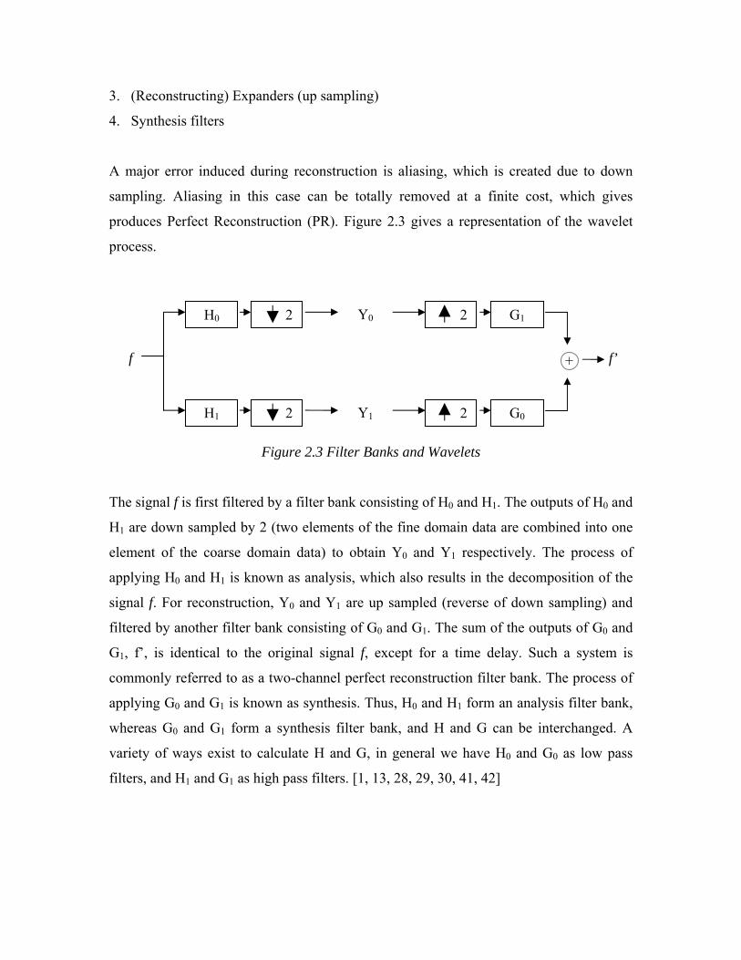
A major error induced during reconstruction is aliasing, which is created due to down

sampling. Aliasing in this case can be totally removed at a finite cost, which gives

produces Perfect Reconstruction (PR). Figure 2.3 gives a representation of the wavelet

process.

Figure 2.3 Filter Banks and Wavelets

The signal f is first filtered by a filter bank consisting of H0 and H1. The outputs of H0 and

H1 are down sampled by 2 (two elements of the fine domain data are combined into one

element of the coarse domain data) to obtain Y0 and Y1 respectively. The process of

applying H0 and H1 is known as analysis, which also results in the decomposition of the

signal f. For reconstruction, Y0 and Y1 are up sampled (reverse of down sampling) and

filtered by another filter bank consisting of G0 and G1. The sum of the outputs of G0 and

G1, f’, is identical to the original signal f, except for a time delay. Such a system is

commonly referred to as a two-channel perfect reconstruction filter bank. The process of

applying G0 and G1 is known as synthesis. Thus, H0 and H1 form an analysis filter bank,

whereas G0 and G1 form a synthesis filter bank, and H and G can be interchanged. A

variety of ways exist to calculate H and G, in general we have H0 and G0 as low pass

filters, and H1 and G1 as high pass filters. [1, 13, 28, 29, 30, 41, 42]

H0

H1 G0

G12

2

2

2

Y0

+

Y1

f f’

2.5 Interpolation for refining

Subsampling is a process of deriving a low resolution data from a high resolution data. It

reduces spatial resolution by taking samples that cover larger areas than the original

samples. For example, a subsampled data may contain one point that represents four

points in the original data. While reconstructing the data from a subsampled data, various

interpolation techniques are used to create the missing points of data thus going from

lower resolution to higher. For our case, we have used three interpolation techniques that

have been discussed below.

2.5.1 Linear interpolation

Linear interpolation is a method of predicting unknown values if we know two

particular values and assume that the rate of change is constant. This prediction is done

by effectively drawing a straight line between two neighboring samples and returning the

appropriate points along that line.

For linearly interpolating a point in the middle of two given points, it will simply

be the average of the given two points. Given f(x) at points x=0,1,2,…, a general formula

for linear interpolation between two points ‘n’ and ‘n+1’ is given as:

( ) (1 ). ( ) . (f n f n f nρ ρ ρ+ = − + +1) - (eq. 2.1)

where:

ρ : 0 1ρ≤ ≤ , represents how far we want to interpolate a signal ‘f’ between time

‘n’ and ‘n+1’.

The interpolation error i.e. ( ) (f n f n )ρ ρ+ − + is nonzero except when ‘f’ is a linear

function between ‘n’ and ‘n+1’. Using eq. 2.1, we can interpolate more than one point

between two given points.

2.5.2 Lagrange Interpolation

Lagrange interpolation is a polynomial interpolation method where an Nth –order

polynomial interpolates N+1 points. The interpolated polynomial passes through the N+1

points. Given a set of N+1 known samples i.e. ( ), 0,1,2,...,kf x k N= , the unique Nth –

order polynomial y(x) which interpolates the specified sample points is given as:

0( ) ( ) ( )N

kky x l x f x

== k∑ - eq. 2.2

where lk(x) is given as:

0

( )( )( )

Ni

ki k ii k

x xl xx x=

≠

−=

−∏

or in the expanded form as:

0 1 1 1

0 1 1 1

( )( )...( )( )...( )( )( )( )...( )( )...( )

k k Nk

k k k k k k k N

x x x x x x x x x xl xx x x x x x x x x x

− +

− +

− − − − −=

− − − − − - eq. 2.3

It is important to note that a first order case of Lagrange Interpolation is the same as

linear interpolation. An advantage of Lagrange Interpolation is that it does not require the

sampled points to be evenly spaced.

2.5.3 Piecewise cubic hermite interpolating polynomial

The Linear and Lagrange interpolation have some drawbacks for which they cannot be

used in every case. Linear interpolation, being very simple, is not suitable for all cases as

it gives less accuracy where data is not changing at a constant rate. On the same, when

we have a large data vector with thousands of data points, the Lagrange formula (eq. 2.3)

gives a high degree polynomial. A better alternative to using a high degree interpolant is

to use several low-degree interpolants, which is the base concept of piecewise polynomial

interpolation.

Let, we have an interval I=[x1,xn], which is divided into n cells, the i-th being Ii=[xi,xi+1]

of length h=xi+1-xi. With f(x) given for all values of x, we seek n polynomials

( ), 1, 2,...,ip x i n= , such that ( )ip x interpolates on the cell [xi,xi+1] and all polynomials

have the same degree. This approach is known as piecewise-polynomial approximation.

Hermite interpolation finds a polynomial p(x) that interpolate f(x) and a polynomial p’(x)

that interpolate f’(x) when f(x) and f’(x) are given at each data point xi, i=1, 2, …, n (‘

represents the first derivative). This can be presented as,

( ) ; '( ) ', 1, 2,...,i i i ip x y p x y i n= = = One method of finding the Hermite interpolation polynomial is using the Lagrange

Interpolation formula, which is given below.

1 1

2

2

0 1 1 1

0 1 1 1

( ) ( ) ' ( )

where( ) (1 2 ' ( )( )) ( )

( ) ( ) ( )( )( )...( )( )...( )( )

( )( )...( )( )...( )

n nn i i ii i i

i i i i i

i i i

i i ni

i i i i i i i n

H x y h x y h x

h x l x x x l x

h x x x l xx x x x x x x x x xl x

x x x x x x x x x x

= =

− +

− +

= +

= − − ×

= − ×

− − − − −=

− − − − −

∑ ∑

A better approximation than the above Lagrange Interpolation method is given by Cubic

Hemite Interpolation and piecewise interpolation, to find a polynomial with a less degree.

Hemite piecewise polynomial interpolation is thus a local interpolation where the

polynomial p(x) on each subinterval [xi-1, xi] is determined by its interpolation data. A

Cubic Hermite Interpolation Polynomial has a degree of four, which using the divided

differences method is given as

1

1

1

11

1

12

12 2

1 1 1 1 1 1

For [ , ], 1, 2,...,( ) ( )

'( )

'( ) 2 '( )( )

( ) ( ) '( ) ( ) ( ) (

i i

i i

i i

ii

i i

i ii

i i

i i i i i i

x x x i nf x f xF

x xF f xF

x xf x F f xF

x x

H f x x x f x x x F x x x x F

−

−

−

−−

−

−

−

− − − − − −

∈ =−

=−

−=

−− +

=−

= + − + − + − − )i i

- (eq. 2.4) Figure 2.4 shows the difference between linear interpolation and cubic hermite piecewise polynomial interpolation.

-3 -2.5 -2 -1.5 -1 -0.5 0 0.5 1 1.5 2-1.5

-1

-0.5

0

0.5

1

1.5

data

linear

hermite

Figure 2.4 Comparison of Linear and Cubic Hermite Piecewise Interpolation

2.6 Taylor Series

Taylor series is a series expansion of an infinitely often differentiable real or complex

function about a point. A Taylor series expansion of a function ( )f x about a point x=a is

given as: ( )

0

( )( ) ( )!

nn

n

f af x xn

∝

== −∑ a - (eq.2.5)

where ( ) ( )nf a represents nth derivative at point a. Expanding eq. 2.5 gives the following:

2 21 ( )( )( ) ( ) ( )( ) ...

2!f a x af x f a f a x a −

= + − + + - (eq. 2.6)

2.7 Finite Difference

Finite difference is the discrete analog of the derivative. The derivative of a function f at a

point x is defined as:

0

( ) (limh

)f x h f xh→

+ − - (eq. 2.7)

As h approaches zero, eq. 2.7 is known as the finite difference, which approaches the

differential quotient. Thus we can use finite differences to approximate derivatives.

2.7.1 Finite difference on regular grids using Taylor Series

In this section, we use the Taylor Series expansion to find the finite difference. We

assume that the sampled points are evenly spaced.

Given evenly sampled data points at discrete points xi, , where points are separated

by a distance of ‘h’ i.e. h=

0i ≥

1i ix x+ − . Thus,

0ix x ih= +

Thus, the discrete representations of the continuous function ‘f’ are:

1 1( ) , ( ) , ( )i h i i i i h if x f f x f f x− − +→ → → f +

Calculating finite difference at xi+1 about point xi, i.e. substituting

1

1

,,

- -

i

i

i i

x xa x

h x x x a

+

+

==

⇒ = =

into eq. 2.6 gives 2 2

11 ...

2!i

i i if hf f f h+ = + + + - (eq. 2.8)

Similarly, calculating finite difference at xi-1 about point xi, i.e. substituting

1

1

,,

- ( )

i

i

i i

x xa x

h x x a x x a

−

−

==

⇒ = = − = − −

into eq. 2.6 gives 2 2

11 ...

2!i

i i if hf f f h− = − + − - (eq. 2.9)

Rearranging eq. 2.8 and eq. 2.9 respectively we have:

1 1 ( )i if ff O hh

+ −= + - (eq. 2.10)

1 1 ( )i if ff O hh

−−= + - (eq. 2.11)

Subtracting eq. 2.9 from eq. 2.8 and rearranging gives:

1 21 1 ( )2

i if ff O hh

+ −−= + - (eq. 2.12)

where 1f represents first derivative, eq. 2.10 represents Forward Difference

Approximation, eq. 2.11 represents Backward Difference Approximation, eq. 2.12

represents Central Difference Approximation and represents higher order

differences. The central difference formula is more accurate with truncation errors of the

order h

( )O h

2.

Taking up the more accurate formula i.e. central difference, adding eq. 2.9 from eq. 2.8

and rearranging gives:

2 21 12

2 ( )i i if f ff O hh

− +− += + - (eq. 2.13)

Eq. 2.13 gives a formula for finding the second derivative of f.

2.7.2 Finite difference on irregular grids

The finite difference method described in the previous section was built on the

assumption that the sampled points are evenly spaced. In our case, as we sample

adaptively, we get cases where sampled points are unevenly spaced i.e. non-uniform.

Data points in a grid can be visualized as follows.

Data pts 0 1 2 i-1 i i+1

h h hh

Uniform sampled points

Data pts 0 1 2 i-1 i i+1

Figure 2.5 Uniform and Non-uniform sampled points

h1 hih0 hi-1

Non-uniform sampled points

2.7.2.1 Using Taylor Series

In this section, we use Taylor Series to find finite difference on irregular meshes. To

calculate expansion of f at xi+1 about the point xi, substituting

1

1

,,

-

i

i

i i

x xa x

h x x h

+

+ i

==

⇒ = =

in eq. 2.6, we have 2 2

11 ...

2!i i

i i i if hf f f h+ = + + + - (eq. 2.14)

Similarly, for f at xi-1 about the point xi, substituting

1

1 1

,,

-

i

i

i i i

x xa x

h x x h

−

− −

==

⇒ = = −

in eq. 2.6, we have 2 2

1 11 1 ...

2!i i

i i i if hf f f h −

− −= − + − - (eq. 2.14)

Subtracting eq. 2.15 from eq. 2.14 and rearranging gives

1 21 1

1

( )i i

i i

f ff O hh h+ −

−

−= +

+ - (eq. 2.15)

Compared to the central difference first derivative formula for uniform grid (eq. 2.12),

eq. 2.15 contains truncation errors as higher order terms do not cancel out due to the non-

uniformity of the unevenly spaced mesh intervals.

To derive the second derivative, we first express first derivatives at mid points of the

mesh intervals, i.e. at 12

i + and 12

i − . Substituting into eq. 2.15, we have

1 211 12 2

( )2

i i

i i

h hf f f O h−

+ −

⎡ ⎤ +⎛ ⎞= − +⎢ ⎥ ⎜ ⎟⎝ ⎠⎣ ⎦

- (eq. 2.16)

As 2 1 1( )f f f= , thus differentiating eq. 2.16, we have

1 1 1 11 12 2

1 1 11 12 2

( )2

( ) ( )2

i i

i i

i ii i

h hf f f f f

h hf f f f

−

+ −

−+ −

⎛ ⎞⎡ ⎤ +⎛ ⎞= −⎜ ⎟⎢ ⎥ ⎜ ⎟⎜ ⎟⎝ ⎠⎣ ⎦⎝ ⎠+⎛ ⎞⎛ ⎞= −⎜ ⎟ ⎜ ⎟⎝ ⎠ ⎝ ⎠

with truncation errors of order h2. Using eq. 2.16 for finding difference, we have

2 21 1 1

1

( )2

i i i i i i

i i

f f f f h hf O hh h

+ − −

−

⎡ ⎤− − +⎛ ⎞= − +⎢ ⎥ ⎜ ⎟⎝ ⎠⎣ ⎦

which is the formula for second order difference for non-uniform meshes. As expected,

substituting hi=hi-1 gives eq. 2.13.

2.7.2.2 Using Lagrange Interpolation An alternative to using the Taylor’s series for finding the second derivative on non-

uniform meshes is through lagrange interpolation. It is interesting to note that this method

does not require interpolating all points, yet it builds on the lagrange interpolation

principle.

Let ti=ih, we use three point interpolation. We have three points

, Thus using lagrange interpolation, we have 1 1 1 1( , ), ( , ) and ( , )i i i i i it f t f t f− − + +

1 1 1 11 1

1 1 1 1 1 1 1 1

( )( ) ( )( ) ( )( )( )( ) ( )( ) ( )(

i i i i i it i i i

i i i i i i i i i i i i

t t t t t t t t t t t tf f f ft t t t t t t t t t t t

+ − + −− +

− − + − + + − +

− − − − − −= + +

− − − − − − ) - (eq. 2.17)

Differentiating eq. 2.17 with respect to ‘t’, we have

1 1 1 1 11 1

1 1 1 1 1 1 1 1

( ) ( ) ( ) ( ) ( ) (( )( ) ( )( ) ( )(

i i i i ii i i

i i i i i i i i i i i i

t t t t t t t t t t t tf f f ft t t t t t t t t t t t

+ − + −− +

− − + − + + − +

− + − − + − − + −= + +

− − − − − −))

i - (eq. 2.18)

Differentiating eq. 2.187 with respect to ‘t’ gives us the second derivative as

21 1

1 1 1 1 1 1 1 1

2 2( )( ) ( )( ) ( )(i i i

i i i i i i i i i i i i

f f f ft t t t t t t t t t t t− +− − + − + + − +

= + +− − − − − −

2)

- (eq. 2.19)

Eq. 2.19 gives the second derivative formula for non-uniform discrete meshes. For

uniform meshes, , substituted in eq. 2.19 gives 1 1i i i it t t t h− +− = − =

21 12 2

2 22 2i i if f f f

h h−= + +− 2

2h+ - (eq. 2.20)

which is the second derivative representation on regular grids using the Lagrange

Interpolation.

2.8 Related work

Compressing the prodigious datasets generated by scientific simulations is an ever

growing problem. Various strategies have been employed to compress this data for

subsequent visualization [10, 11, 13, 14]. Analysis and post processing usually makes use

of taking spatial derivatives, the required tolerances usually exceed that of visualization

itself. One work around is to use lossless compression [12, 9], but compression is

generally limited to a factor of two at best.

Subsampling is a lossy technique used for compression in large regular gridded scientific

datasets. Representing the original data with a hierarchical representation has been

employed [1] using the wavelets [13, 28, 29, 30, 41, 42] in the past. On the same,

Spatially Adaptive Subsampling of Image Sequences has also been studied [4].

Like wavelet compression, adaptive coarsening is a multiresolution technique; however,

it does not represent data progressively. Similarly, Adaptive coarsening is similar to

adaptive sub-sampling employed in High Definition TV signal processing [4], which

splits the index domain into fixed size pieces and subsamples each piece separately. This

simpler but constrained sub-sampling procedure comes at a cost: compression drops. At a

threshold of 10−3 adaptive coarsening provides a much better compression.

3 Method & Implementation For our purposes, we only concentrate on spatial compression.

3.1 Sub Sampling Subsampling is one of the most basic lossy data compression methods. It derives a lower-

resolution data from a higher-resolution data. The original high resolution data, which

may be over sampled, is compressed by discarding a part of the data points. Figure 3.1

explains the process of subsampling.

(a)

Original block of data Subsampled at: lev=1 lev=2

(b) Figure 3.1 Subsampling in (a) one dimension (b) two dimension

One method of applying subsampling is fixed subsampling. In this method, a predefined

level of subsampling or fixed lattice is applied to the original data. By applying the same

level of subsampling, either we achieve less compression (where a higher level of

subsampling could have been applied) or otherwise exceed the tolerance level in some

portions of the data (where high resolution is needed to represent the original data).

Adaptive subsampling, as the name suggests, adaptively subsamples the data, using lower

level of subsampling at detailed regions of the original data and high level of

subsampling at portions that have lesser details. The original mesh is coarsened, and then

the result is re-refined using any suitable interpolation technique. If the re-refined data

approximates the original data to a sufficient accuracy (given as a tolerance level), it

suggest that the data can be further coarsened. This process is carried out recursively,

with coarsening newly coarsened data, until further coarsening is not possible. This

happens when either the tolerance level is exceeded or we are left with a single panel of

data. Adaptive subsampling can be further classified as Fixed Interval and Adaptive

Coarsening.

3.1.1 Fixed Interval algorithm The Fixed Interval (FI) method is based on adaptive subsampling where the original data

is divided into intervals of predefined fixed size. Each interval is then subsampled

adaptively to a maximum amount, as permitted by a pre-decided tolerance value. Given a

dataset D of size ‘n’, an interval size ‘iSize’ and tolerance level ‘tol’, the Fixed Interval

Algorithm is given below.

1 divide D into intervals I of size iSize 2 for each interval Ii, do 3 for lev=2 to maxLev, do 4 coarsen Ii to level lev; define as Ci,lev 5 refine Ci,lev using interpolation; define as Ri,lev 6 if relative error(Ci,lev - Ri,lev) < tol continue with next lev (goto 3) 7 else goto 2 (*maximum coarsening achieved for this interval*) 8 end for 9 end for each

Figure 3.2 Fixed Interval Algorithm

In step 1, we divide D into ‘k’ intervals, where k=n/iSize. The divided intervals are

represented as Ii, i=1,2,…,k. On step 5, we can use any of the interpolation techniques

discussed in the background chapter. If the condition on step 6 is true, it means that the

data in the particular interval can be coarsened till the current level, as is then tried for a

next level of coarsening by going to step 3. It is important to note that we use the relative

error metric (step 6) to compare original data and the re-refined data. We will use this

throughout our experiments.

We use the following standard variable names throughout the listings. This is also

available in Appendix at the end of the report.

nsnaps= Number of snapshots in the dataset to compress n = Number of points in each snapshot tol = Tolerance iSize = Interval size dt = Distance between two consecutive data points nInt = Number of Intervals nlev = Number of levels The pseudo code of applying FI on one dimensional data is given in Figure 3.3.

The algorithm for FI on two dimensional data is almost the same, with using coarsening

in two dimension and re-refining/interpolation in two dimensions. In our case, for better

compression in two dimensional data, we use a hybrid approach of FI and AC, which is

described in a later section.

For FI, we use a predefined interval size. As our results (discussed in the next chapter)

show, we get different overall compression using different interval sizes on the same

original dataset. Thus, choosing an optimal interval size for a particular type of dataset is

important.

1 compress(file,tol,iSize) 2 begin 3 NTot = 0 4 CTot = 0 5 for k = 0 to nspans 6 ds = readstep(file, n) 7 cdata = coarseNcompress(ds,n,tol,iSize) 8 cn = countpoints(cdata) 9 NTot = NTot+n 10 CTot = CTot+cn 11 end for 12 overallCompression = NTot/CTot 13 end ---------------------------------------------------------- 14 coarseNcompress(u,n,tol,iSize) 15 begin 16 nInt = n/iSize 17 nlev = log2(iSize) 18 cCells = cell(1,nInt) 19 for curInt=1 to nInt 20 cCell{curInt} = refin(u,n,tol,intSize,curInt) 21 end for curInt=1 to nInt 22 return cCells 23 end ---------------------------------------------------------- 24 refin(u,n,tol,iSize,curInt) 25 begin 26 offset = (curInt-1)*intSize; 27 original = u(offset+1:offset+intSize) (*original interval*) 28 for lev = nLev to 1 29 cPt = coarsen(original,lev) (*take the coarsened points*)

30 Ureref = refine(cPt, lev) (*Refine the interval*)

31 (*Compare tolerance level*) 32 Mdiff = abs((orignal- Ureref)./original) < tol; 33 if(allones(Mdiff)) 34 return cPt 35 end 36 if lev == 2 (*all iterations done*) 37 return original 38 end 39 (*apply next level of coarsening*) 40 end 41 end

Figure 3.3 Pseudo code for the Fixed Interval Algorithm

3.1.2 Adaptive Coarsening algorithm The Adaptive Coarsening (AC) algorithm compresses data non-uniformly according to a

recursive error analysis procedure. AC breaks down the original data into non-uniform

length intervals, in contrast to FI which divides the data into equal length intervals. The

divided intervals in both cases i.e. FI and AC are compressed to different levels.

Let the dataset D of size ‘n’, defined on data points i, where i=1,2,...,n (‘i’ basically

represents an index space over which D is defined) is to be compressed to a tolerance

level of ‘tol’. The algorithm recursively compresses D for each level of subsampling and

stores the result in an array ‘levels’; ‘levels’ stores the indexes that can be coarsened to

that level. The algorithm follows.

1 let levels[0]= u(h) 2 for lev = 1 to maxLev 3 hlev = coarsening to level lev; 4 for each subdomain uj(hlev-1) in levels[lev-1] do 5 where error(uj(hlev-1)) < tol, generate a new coarse domain uj(hlev) 6 levels[lev] = levels[lev] U uj(hlev) 7 end for each 8 end for

Figure 3.4 Adaptive Coarsening Algorithm

On line 6, U represents the set union operator. Similarly, u(hlev) represents the original

data points coarsened to level represented by hlev. Thus u(h) represents the original data

i.e. coarsened to lev=0 which is infact the original data, while u(h1) will mean coarsened

to level 1. The error is checked on line 5 and the appropriate portions of the mesh are

coarsened; these portions can be disjoint. The portions that can be coarsened are

augmented using the set union operator on line 6.

The pseudo code for the Adaptive Coarsening Algorithm is given in Figure 3.5.

compress(file,tol,iSize,dt,C,IMin) begin NTot = 0 CTot = 0 do k = 0,nspans ds = readstep(file, n) Uc = coarsen(ds,C,n) levels = compression(Uc,C,tol,n,IMin) cn = countpoints(levels) NTot = NTot+n CTot = CTot+cn end do overallCompression = NTot/CTot end

1. compression(Uc,C,tol,n,IMin) 2. begin 3. levels = cell(1,nlev); 4. levels{1} = [1 n]; 5. for lev = 2:nlev 6. FLevel = levels{lev-1}; 7. for each FIntv element of levels{lev-1} 8. if ((FIntv(2) - FIntv(1)) < IMin*C) 9. continue; 10. end 11. [icstart, icend] = calcoarseindexes(FIntv,C,n) 12. [iostart, ioend] = caloriginalindexes(FIntv,C,n) 13. cU = getcoarse(Uc,icstart,icend) 14. oU = getoriginal(Uc,iostart,ioend) 15. Cr = C^(lev-1); 16. Urerefined = Refine(cU, Cr); else 17. Mdiff = abs( (Urerefined - oU )/oU) < tol; 18. [starts,ends] = generatestartnend(Mdiff,Cr,n) 19. [starts,ends] = removeshortintervals(starts,ends,IMin) 20. [starts,ends] = normalizeinterval(FIntv,C,starts,ends) 21. levels{lev} = [levels{lev}; [starts,ends] ]; 22. end 23. end 24. return levels 25. end

Figure 3.5 Pseudo code for the Adaptive Coarsening Algorithm

A brief description of some of the lines in Figure 3.5 are given below.

line 8-10 Ignore empty intervals, or intervals that are smaller than IMin line 16 Refine the coarsened interval line 17 Compare with the corresponding portion of the original interval line 18 Generate indexes of start and end intervals based on the logical vector Mdiff. A sequence of logical ones in Mdiff represents an interval that can be coarsened while logical zeros mean that the portion doesn’t meet the error bound, and thus cannot be coarsened line 19 Delete intervals that are shorter than IMin points line 20 Normalize start and end points to that level line 21 Insert interval descriptors for the newly created coarse intervals and append to current level

3.2 Finite Difference Knowing in advance how the data will be manipulated can be employed in the

compression process to guarantee error bounds on the manipulations. This was one of the

goals of our experiments. For this purpose, we used derived quantities like the second

derivatives to a specified accuracy.

We use the following abbreviations for the documentation to follow:

O = Original data

D = Second derivative

C = Coarsening data

R = Reconstructing/Re-refining data

Combining the above in sequence, we get abbreviations that depict the overall process

which have been summarized in the following table.

Abbreviations Meanings

OD Applying second derivative to the original data

OCRD Coarsening original data, followed by re-refining and then applying

second derivative on the compressed reconstructed data

ODCR Applying second derivative to the original data, then applying

coarsening and re-refining on the result of the second derivative

OCDR Coarsening original data, and then applying second derivative on the

coarsened data, followed be re-refining the differentiated coarsened data

The above three sequence of operations (OCRD, ODCR, OCDR) give all the possible

combinations of the D, C and R operations. Comparing the results of these three gives us

a better idea as to which sequence is best to use to achieve highest level of compression

while guaranteeing an error bound on the results. As our results show, compressing the

differentiated data (ODCR) doesn’t produce the best results which is explained by how

the second derivative affects the properties of the data. All discussion on this is the topic

of the next chapter. While reading the sections to follow, the reader should keep in mind

that the goal of this exercise is to compress differentiated data to a specified tolerance

level.

3.2.1 OD We used the formulas derived in the previous chapter to take the derivative of the discrete

data. For finding the second derivative on uniform data, we used two formulas based on

the Taylor Series expansion. The first formula uses two neighboring points, and is thus

second order accurate.

( ) 21 12i i i if f f f− += − ∗ + h

While the second formula involves four neighboring point and is thus fourth order

accurate.

( ) 22 1 1 216 30 16 (12 )i i i i i if f f f f f− − + += − + ∗ − ∗ + ∗ − ∗h

For non-uniform meshes, we used one formula based on Taylor series and one based on

Lagrange interpolation. The formula for second derivative on unequal spaced data using

Taylor Series is

3212)(3

)(2

,)(1

1

11

1

)/c -c (c derv,hh c

,hff c

hff c

i

ii

jii

jii

=+=

−=

−=

−

−−

+

and Lagrange Interpolation is

321232221

1111

11

1111

cc c derv,) )-t) * (t-t( (tf c

,) )-t) * (t-t( (tf c,) )-t) * (t-t( (tf c

i

iiiii

iiiii

ii-ii-i

++=∗=∗=∗=

+−++

+−

+−

After experimenting, we observed that using these formulas doesn’t yield considerable

compression. Consequently, we used a modified formula of uniform mesh on the non-

uniform mesh. We discuss our modified approach in the section entitled OCDR, as we

get non-uniform meshes only in this case.

3.2.2 OCDR OCDR involves the following steps

1. Coarsening original data, producing OC

2. Taking second derivative of the coarsened data, resulting in OCD

3. Re-refining differentiated data i.e. OCD to produce OCDR. This re-refined data is

compared with OD. If OCDR interpolates OD to the given error bound, go to step

1 and apply next level of coarsening.

Applying the differentiation operation on coarsened data is one of the properties that are

not applicable to all types of compression. Thus, one of the major advantages of using

subsampling is its property to apply numerical techniques directly on the compressed

coarsened data. For practical purposes, we can thus coarsen data to a filtered out level

and store only the coarsened points. When using, we can apply the operations like

differentiation on the coarsened data, and then re-refining gives results to our initial error

bound.

For FI, the original data O is divided into predefined interval sizes, and then the above

steps are executed on each interval individually. The comparison in the third step is thus

between OCDR and OD for that interval.

The original data O is divided into intervals after a first iteration of the afore mentioned

three steps in the case of AC. After applying OCDR for the first iteration, it is compared

with the complete OD. This gives an idea of which parts of the data can be coarsened

further, and which cannot. Thus, the portions of the data that can be coarsened further are

the subject for the next iterations, while the comparison made in the next iterations is

with the corresponding intervals in OD. The pseudo code for OCDR is given in appendix.

3.2.3 ODCR As discussed previously, ODCR means

1. Taking second derivative of the original data, producing OD

2. Coarsening OD, resulting in ODC

3. Re-refining ODC, resulting in ODCR. If ODCR represents OD to the specified

error bound, go to step 2 and apply the next level of coarsening

ODCR is quite similar to the normal compression method, the only difference being that

we give as input the differentiated data instead of the original data. Thus, the algorithm is

same as simple compression for both AS and FI.

3.2.4 OCRD OCRD applies the following steps on the original data:

1. Coarsen original data, producing OC

2. Re-refining the coarsened data, producing OCR

3. Taking second derivative of the re-refined data OCR, producing OCRD. Compare

OCRD with OD, if OCRD represents OD to the specified error bound, go to step

1 and apply next level of coarsening.

For FI, this process (applying all three steps) is carried out on each divided interval

individually. This also means that the comparison on the third step is done with the

respective interval of the already calculated OD.

We have a modification for AC, where initially, step 1 and 2 are applied on all the data.

After the comparison in step 3, only intervals that can be coarsened further, which is

decided based on which points meet the error bound, are worked on in the next recursion

step i.e. applying the three steps again. This time, the comparison is made between

OCRD for the selected interval and OD for the respected interval.

It is important to note that for OCDR and OCRD, we need to re-adjust the data before

applying the second derivative. The reason for this is that taking second order second

derivative of n-data points yields n-2 data points, while taking the fourth order second

derivative yields n-4 data points. For now, we will talk about using the second order

second derivative only. The same concepts have been used for the fourth order formula in

the implementation but have not been explained here.

Once the data is divided into intervals, when we differentiate an interval of size p, we get

p-2 points. For final results, we expect OCDR and OCRD to interpolate OD to the given

error bound, thus for the interval, we have to compare it with p points in OD. For this

purpose, we add a data point on each end known as a ghost cell. The ghost cell is filled

either by interpolation or by subsampling depending on the level of coarsening used on

that side. This will give p+2 points, which when differentiated give p points. This is then

compared to OD. It is important to note here that, depending on the neighboring intervals,

we may either have the data point which we need (incase the neighboring interval is less

coarsened) or we will have to interpolate the data point (incase the neighboring interval is

more coarsened). Figure 3.6 attempts to explain this discussion.

OD on n points gives n-2 points. Similarly for OCDR and OCRD, we don’t interpolate to

the left for the first interval and right for the last interval. This adjusts the data points.

Figure 3.6 Interpolating for taking derivative

OOD

No ghost cell needed on left side of interval

No ghost cell needed on right side of interval

Uneven Coarsened Data If points on the left are coarsened with h, and points on the right with 2h: +-----+-----+-----+-----------+------------+-----------+ (‘+’ represents a data point) Divide into 2 pieces, (‘o’ represent ghost cells) +-----+-----+-----+-----o o------------+-----------+------------+-----------+

ghost cell filled by interpolating in between two endpoints of the neighboring ghost cell.

ghost cell filled by subsampling.

3.3 Sub Sampling on two dimensional data For the two dimensional data, we use a hybrid approach of FI and AS. We use block

distribution to divide the original data into predefined fixed sized blocks. This is

analogous to the FI method. This is shown in Figure 3.7.

Each block is then coarsened as described in the section of subsampling of two

dimensional data. Re-refining the coarsened data in two dimensions also requires two

dimensional interpolation (we used spline method of 2d interpolation). The re-refined

blocks are then compared to the original blocks; blocks that interpolate the original data

to a specified error bound are subject to further coarsening in the next iteration.

1 2 3 4

5 6 7 8

9 10 11 12

13 14 15 16 Block

Block Full Figure 3.7 Block distribution

When we coarsen and re-refine the blocks for the first time i.e. for level=1, we check

against original data. If a block does not interpolate to the specified tolerance level, the

block number is recorded. Thus, after the first iteration, we have an array ‘bUncoarsened’

with block numbers that cannot be coarsened (coarsened) even to the first level.

These blocks, if not compressed, reduce the overall compression a lot thus we aim to

some how compress these blocks. It is important to note also that these blocks also

represent the regions of the data that has data that changes too rapidly, or noise otherwise.

For example, in a situation where we have rapidly changing data in the middle will have

a structure like Figure 3.8.

1 2 3 4 5 6 7 8 9 10 11 12 13 14 15 1617 18 19 20 21 22 23 24 25 26 27 28 29 30 31 3233 34 35 36 37 38 39 40 41 42 43 44 45 46 47 4849 50 51 52 53 54 55 56 57 58 59 60 61 62 63 6465 66 67 68 69 70 71 72 73 74 75 76 77 78 79 8081 82 83 84 85 86 87 88 89 90 91 92 93 94 95 9697 98 99 100 101 102 103 104 105 106 107 108 109 110 111 112

113 114 115 116 117 118 119 120 121 122 123 124 125 126 127 128129 130 131 132 133 134 135 136 137 138 139 140 141 142 143 144145 146 147 148 149 150 151 152 153 154 155 156 157 158 159 160161 162 163 164 165 166 167 168 169 170 171 172 173 174 175 176177 178 179 180 181 182 183 184 185 186 187 188 189 190 191 192193 194 195 196 197 198 199 200 201 202 203 204 205 206 207 208209 210 211 212 213 214 215 216 217 218 219 220 221 222 223 224225 226 227 228 229 230 231 232 233 234 235 236 237 238 239 240241 242 243 244 245 246 247 248 249 250 251 252 253 254 255 256

Figure 3.8 bUncoarsened

Where green blocks represent blocks that are coarsened to a maximum level and yellow

blocks represent blocks that are not coarsened at all. The numbers represent the block

number, a total of 256 blocks.

The overall compression for just the green blocks is very high. We tried the following to

compress the yellow blocks.

1. As in quad trees, I tried to divide the 16x16 yellow blocks into quadrants and then

coarsen but this also didn’t work as the points that could not be coarsened were

distributed in all quadrants.

2. The other solution was to combine the blocks either in the x-direction or y-

direction to get a single one dimensional array of points and then apply the AC

algorithm on it. Combining the above blocks row wise gives

1 2 3 4 5 6 7 8 9 10 11 12 13 14 15 16

17 18 19 20 21 22 23 24 25 26 27 28 29 30 31 3233 34 35 36 37 38 39 40 41 42 43 44 45 46 47 4849 50 51 52 53 54 55 56 57 58 59 60 61 62 63 6465 66 67 68 69 70 71 72 73 74 75 76 77 78 79 8081 82 83 84 85 86 87 88 89 90 91 92 93 94 95 9697 98 99 100 101 102 103 104 105 106 107 108 109 110 111 112

113 114 115 116 117 118 119 120 121 122 123 124 125 126 127 128129 130 131 132 133 134 135 136 137 138 139 140 141 142 143 144145 146 147 148 149 150 151 152 153 154 155 156 157 158 159 160161 162 163 164 165 166 167 168 169 170 171 172 173 174 175 176177 178 179 180 181 182 183 184 185 186 187 188 189 190 191 192193 194 195 196 197 198 199 200 201 202 203 204 205 206 207 208209 210 211 212 213 214 215 216 217 218 219 220 221 222 223 224225 226 227 228 229 230 231 232 233 234 235 236 237 238 239 240241 242 243 244 245 246 247 248 249 250 251 252 253 254 255 256

Figure 3.9 Marked bUncoarsened where each color represents the combined block. We then changed these

combined blocks into 1d by concatenating their rows. Thus row 1 of block 71 is

followed by row 1 of 72, then 73 and then 74. This is followed by row 2 of block

71, then row 2 of 72 and so on. We aimed at using the property of the generated

data that the data changes slowly in the x-direction. To confirm this behavior with

an example, we chose the third block i.e. 103 to 110. The 2D view is for block

103 to 110 is

Figure 3.10 2d view of blocks 103-110

Concatenating rows gives:

Figure 3.11 Blocks 103-110 concatenated in the X-dir

Concatenating columns gives:

Figure 3.12 Blocks 103-110 concatenated in the X-dir

As can be seen, concatenating rows (x-direction) shows slower changing data than

concatenating column (y-direction). Thus, we combined the blocks in the rows by

concatenating their rows. We then applied the normal 1d AC algorithm on the

concatenated one dimensional data. This is why I initially choose to concatenate

rows. In our discussion of results in the next chapter, we give readings that show

the ration of compression that we achieve by using this hybrid approach of using

FI and AC.

The data set used for our two dimension compression is already differentiated,

thus it is a case of ODCR.

4 Analysis In this chapter, we present our results of the experiments mentioned in the previous

chapter, along with motivation for the experiments and a discussion covering our

interpretation of the results. The sections in this chapter only present the graphs based on

the results. For full values, refer to appendix. Based on the design of the experiments, we

divide our results in this chapter into five categories:

1. Comparison of compression for different interval sizes in one dimension using FI.

2. Comparison of compression achieved using Linear interpolation and Hermite

cubic piecewise polynomial interpolation using AC

3. Comparison of compression between FI and AC for one dimensional data

4. Context dependent compression, covering ODCR, OCDR and OCRD on one

dimensional data

5. Compression of two dimensional data, including a compression ratio in 1d and 2d

To generate data for one dimension, we carried out the simulation described in section

2.1 on a uniform 1-dimensional mesh with 16,385 points. The timestep was 1.2207 × 10−5

and the simulation ran for 163,840 timesteps. The state of the simulation was written to

disk every 2048 timesteps. Thus, the simulation dataset comprises 81 snapshots, spaced

at equal positions in time, including the initial condition. The total amount of data written

was thus 81*16385*8 (=10,617,480) bytes per double precision floating point number.

Since the metadata (data describing the data) is very less in size compared to the data

itself, thus we don’t include its size in our discussions. We applied the compression

techniques on all 81 snapshots and counted the total number of words written in each

snapshot, which gave us an overall compression value. We also used varied values of the

error threshold, 10-3, 10-4 and 10-5, which are sufficient for engineering precision. We

generated a 1020x1020 points data set for the two dimensional experiments.

4.1 Different interval sizes using FI The FI algorithm depends on the dataset (rate of change of values, range of values etc),

the tolerance level used and the interval size chosen for compression. We used interval

sizes of 32, 64, 128, 256, 512 and 1024. The results have been plotted in Figure 4.1.

0 200 400 600 800 1000 12000

5

10

15

20

25

30

35

40

45Interval size vs. Compression

Interval size

Ove

rall

com

pres

sion

10-5

10-4

10-3

Tolerance:

Interval Size vs. Compression

0

5

1015

2025

3035

40

45

10 -̂3 10 -̂4 10 -̂5

Tolerance

Com

pres

sion

32

64

128

256512

1024

Figure 4.1 Compression using different interval sizes in FI

By dividing the data set into equal sized intervals in FI, we coarsen each interval meaning

that the coarsened points interpolate the whole interval. Thus, as tolerance level

decreases, we need smaller intervals so that better interpolation can be done. This is why

we see that we need smaller interval size for smaller tolerance level. We have

summarized our readings in Table 4.1.

Error bound Best interval size Compression 10-3 128 41.1632 10-4 64 17.0981 10-5 32 6.9147

Table 4.1 Best interval sizes in FI

4.2 Comparison of using pchip and linear interpolation Linear interpolation works well when rate of change of data is constant. This is usually

not the case in scientific simulations. On the other hand, the Hermite cubic piecewise

polynomial interpolation (pchip) method handles the case of varying rate of change of

data well. The difference in compression achieved using the two mentioned methods of

interpolation is given in Figure 4.2.

Linear vs. Hermite(pchip) Interpolation

0

20

40

60

80

100

120

10 -̂3 10 -̂4 10 -̂5

Tolerance

Com

pres

sion

pchiplinear

Figure 4.2 Linear vs. Pchip interpolation using AC

4.3 FI vs AC Our next set of experiments aimed at comparing the compression achieved through FI

and AC using linear interpolation. For the comparison, we choose the best interval size

for each tolerance level based on the results achieved in the previous experiments.

0 20 40 60 80 10020

40

60

80

100

120

140

160

Time step

Com

pres

sion

FIAC

0 20 40 60 80 10010

20

30

40

50

60

Time step

FIAC

0 20 40 60 80 1004

6

8

10

12

14

16

18

Time step

Com

pres

sion

FIAC

AC vs. FI

0102030

405060

10^-3 10^-4 10^-5

Tolerance

Ove

rall

com

pres

sion AC

FI

(a) (b)

(c) (d) Figure 4.3 FI vs AC (a)10-3 (b)10-4 (c)10-5 (d)Comparison

As expected, AC gives more compression than FI, though it is quite less as the tolerance

level decreases. The comparison is summarized in Table 4.2.

Error bound Interval size for FI Compression, FI Compression, AC 10-3 128 41.1632 53.84 10-4 64 17.0981 19.57 10-5 32 6.9147 7.378

Table 4.2 Table 4.2 FI vs. AC

4.4 Context dependent compression One of the objectives of our work was to show that we need to know how the data will be

manipulated numerically, so that we can provide guaranteed error bounds on those

manipulations. Thus, we don't just compress the data, and then operate it at will; rather

we need to be sure that we can obtain derived quantities like second derivatives to a

specified accuracy. To achieve this, we evaluated compression for possible combinations

of coarsening(C), re-refining(R) and the second derivative(D), i.e. ODCR, OCRD and

OCDR. We use two forms of the second derivate: second order accurate and fourth order

accurate. For the FI method, we used intervals of size 64, 128 and 256. We give our

results for each of the above, and end this section with a comparison of the three.

4.4.1 ODCR We use both linear interpolation as well as the hemite cubic piecewise polynomial

(pchip) interpolation; and second order and fourth order accurate second derivative

formulas for ODCR. This gives a complete comparison for ODCR. The rounded off

results have been given in Table 4.3; more accurate results can be found in appendix.

OD22CR OD24CR Error

Bound AS AS-p* FI(64) FI(128) FI(256) AS AS-p FI(64) FI(128) FI(256)10^-3 8.660 10.255 7.305 6.615 5.658 7.594 8.747 6.558 6.000 5.18810^-4 2.606 3.045 2.345 2.212 2.068 2.426 2.792 2.208 2.101 1.97610^-5 1.378 1.652 1.275 1.246 1.216 1.335 1.573 1.237 1.210 1.183

Table 4.3 ODCR

* using pchip

The comparison is given in Figure 4.4.

0

2

4

6

8

10

12

OD22CR OD24CR

Ove

rall

com

pres

sion

ASAS-pFI(64)FI(128)FI(256)

0

0.5

1

1.5

2

2.5

3

3.5

OD22CR OD24CR

Ove

rall

com

pres

sion

ASAS-pFI(64)FI(128)FI(256)

00.20.40.60.8

11.21.41.61.8

OD22CR OD24CR

Ove

rall

com

pres

sion

ASAS-pFI(64)FI(128)FI(256)

Figure 4.4 ODCR for error bound (a) 10-3 (b) 10-4 (c) 10-5

4.4.2 OCDR Our results for OCDR, using both second order accurate and fourth order accurate

formulas, represented as OCD22R and OCD24R respectively, are given in Table 4.4.

OCD22R OCD24R Error Bound AS FI(32) FI(64) FI(128) FI(256) AS FI(32) FI(64) FI(128) FI(256)10^-3 9,928817 7,0398 7,1981 6,1426 4,7094 11,42166 7,322 7,5645 6,4021 4,8039 10^-4 3,621795 3,2181 3,085 2,8606 2,5456 3,856392 3,3325 3,1865 2,9257 2,5502 10^-5 1,521811 1,4153 1,3832 1,3469 1,3023 1,579224 1,4578 1,4238 1,3833 1,3298

Table 4.4 OCDR

The comparison of compression for OCD22R and OCD24R is given in (c)

Figure 4.5.

0

2

4

6

8

10

12

OCD22R OCD24R

Ove

rall

com

pres

sion

ACFI(32)FI(64)FI(128)FI(256)

00,5

1

1,52

2,53

3,54

4,5

OCD22R OCD24R

Ove

rall

com

pres

sion

ACFI(32)FI(64)FI(128)FI(256)

00,2

0,40,60,8

11,21,4

1,61,8

OCD22R OCD24R

Ove

rall

com

pres

sion

AC FI(32)FI(64) FI(128)FI(256)

(a) (b)

(c)

Figure 4.5 OCDR for error bound (a) 10-3 (b) 10-4 (c) 10-5

4.4.3 OCRD If we use the linear interpolation method, it is not possible to take the second derivative

of the reconstructed signal i.e. CR. We explain why using the second order accurate

second derivative formula i.e. D22.

Let, the data points are f1, f2, f3, f4, f5, f6,…,fn . The formula for D22 is:

( ) 21 12i i if f f h− +− ∗ + ; for i=2, we 3 have 1 22f f f− ∗ + (Lets not consider the 1/h2 factor

for the moment).

When we coarsen the data to the first level, we have f1, f3, f5,…,fn . Using linear

interpolation, re-refining the coarsened data gives,

f1, f2=(f1+f3)/2, f3, f4=(f3+f5)/2, f5, ....

Now, substituting this in the formula for D22, we have:

f1-2*((f1+f3)/2)+f3

Solving this gives a 'zero'. On the other hand, hermite cubic piecewise polynomial

interpolation (pchip) does not suffer from this problem, thus we use pchip for

interpolation when evaluating OCRD. We use only the AS method for OCRD; the results

are given in Table 4.5.

Error Bound OCRD24 using AS

10^-3 7.517678 10^-4 2.414907 10^-5 1.34772

Table 4.5 OCRD

4.4.4 Comparison A comparison of the above techniques reveals the following:

• ODCR gives best compression using AC and pchip interpolation

• OCDR gives best compression using AC

• OCRD has only been taken using AC and pchip interpolation

The above mentioned best values have been assembled in Table 4.6.

AS Error

Bound OD22CR-p OD24CR-p OCD22R OCD24R OCRD24 10^-3 10.255393 8.746678 9,928817 11,42166 7.517678 10^-4 3.045141 2.791918 3,621795 3,856392 2.414907 10^-5 1.65211 1.573311 1,521811 1,579224 1.34772

Table 4.6 Comparison of best compression techniques for second derivative The comparison has been plotted in Figure 4.6.

ODCR,OCDR and OCRD

0

2

4

6

8

10

12

10^-3 10^-4 10^-5Tolerance

Ove

rall

com

pres

sion

OD22CROD24CROCD22ROCD24ROCRD24

Figure 4.6 Comparison of best compression techniques for second derivative

The results reveal that we can use OCDR to get maximum compression, yet guarantee a

specified error bound for the second derivative.

4.5 Compression in 2D For compression in 2d, we used an error bound of 10-3 only. We got an overall

compression of 16.414328 out which the 2d FI method contributed a compression of

17.5914 while 1d AC contributed 2.3315 (refer to previous chapter for separation of FI

and AC). If we only would have used 2d FI, without employing 1d AC, we would have

achieved a compression of 14.8856. The results have been summarized in Figure 4.7

which shows the compression for each step.

0 10 20 30 40 50 6010

15

20

25

30

35

Step

Com

pres

sion

Figure 4.7 Compression in 2d

5 Conclusions and future work

This work makes the following contributions: 1) it offers an improved adaptive

subsample procedure for scientific data that trades off added irregularity for improved

compression; 2) its shows how compression increases using the adaptive coarsening

compared to fixed sized intervals method; 3) it establishes the need to compress in the

context of how data will be used in subsequent post-processing. As expected,

compression decreases with the amount of loss, but up to an order of magnitude in

compression was obtainable while retaining engineering precision. Accuracy drops

rapidly as the number of digits increases, and to this end we are investigating more

sophisticated sampling and interpolation procedures. We expect higher compression in

three dimensions, which is currently under investigation. Also, Adaptive coarsening

parallelizes readily as coarsening and refinement procedures require nearest neighbor

communication only. Some collective communication is required to ensure that that the

irregular mesh structure makes balanced use of parallel I/O, but the cost is modest, since

the data block sizes are large. The work can also be extended to give a comparison with

the wavelet compression method, and a standard C library can be built for easy usage.

6 Appendix

6.1 Pseudocode for OCDR General variables used in all pseudo codes

nsnaps= Number of snapshots in the dataset to compress n = Number of points in each snapshot tol = Tolerance iSize = Interval size dt = Distance between two consecutive data points nInt = Number of Intervals nlev = Number of levels ---------------------------------------------------------- Pseudo code for OCDR ---------------------------------------------------------- compress(file,tol,iSize,dt) begin NTot = 0 CTot = 0 do k = 0,nspans ds = readstep(file, n) cdata = coarseNcompress(ds,n,tol,iSize,dt) cn = countpoints(cdata) NTot = NTot+n CTot = CTot+cn end do overallCompression = NTot/CTot end ---------------------------------------------------------- coarseNcompress(u,n,tol,iSize,dt) begin nInt = (n-1)/iSize nlev = (log2(iSize)/log2(2)) cCells = cell(1,nInt) int2c = 1:nInt do lev = 2,nlev newint2c = [] for each curInt Є int2c [cCell{curInt},flag] = refin(u,n,tol,iSize,curInt,lev,dt) if (flag) newint2c = [newint2c curInt] end end for each curInt Є int2c int2c = newint2c end do return cCells; end ----------------------------------------------------------

[resArr,flag] = refin(u,n,tol,iSize,curInt,lev,dt) begin nInt = (n-1)/iSize offset = (curInt-1)*iSize endofInt = offset+iSize cfac = 2^(lev-1) ffac = 2^(lev-2) iv = 1 : ffac : intSize Pts = u(offset+1:endofInt) orig = Pts(iv) iv = 1 : 2 : length(orig) ic = orig(iv) id = secondderivative(orig, dt*ffac) icd = secondderivative(ic, dt*cfac) icdr = Refine(icd, 2) nid = length(id) nicdr = length(icdr) Mdiff = abs((id-icdr)./id) < tol if (allones(Mdiff)) resArr = ic flag=1 else resArr = orig flag=0 end end (* End of pseudo code for OCDR *)

6.2 Readings

Interval Size Error Bound 32 64 128 256 512 1024 10^-3 25.8449 36.9638 41.1632 36.2698 27.3934 17.9833 10^-4 15.4543 17.0981 16.7519 14.9454 12.189 9.002 10^-5 6.9147 6.9031 6.6608 6.1763 5.4574 4.5077

Table 6.1Compression for different interval sizes in FI

AC Error Bound Linear Pchip 10^-3 53.84336 109.062810^-4 19.57154 58.6031310^-5 7.378415 31.32074

Table 6.2Comparison of using pchip and linear interpolation

OD22CR OD24CR Error Bound AS AS-p FI(64) FI(128) FI(256) AS AS-p FI(64) FI(128) FI(256) 10^-3 8.65954 10.25539 7.305262 6.614821 5.657516 7.593902 8.746678 6.55815 6.000154 5.18839510^-4 2.606418 3.045141 2.345012 2.212238 2.068113 2.425562 2.791918 2.207686 2.101113 1.97616210^-5 1.378304 1.65211 1.274708 1.246363 1.216338 1.334798 1.573311 1.236672 1.210491 1.183441

Table 6.3ODCR Full Readings

7 References

1. An Efficient Hierarchical Data Representation Scheme for Gridded Data by John Clyne, Scientific Computing Division, National Center for Atmospheric Research

2. Using Desktop Graphics Workstations for Interactive Remote Exploration of Large Data Sets by Lori A. Freitag and Raymond M. Loy, Mathematics and Computer Science Division, Argonne National Laboratory

3. The Multiresolution Toolkit: Progressive Access for Regular Gridded Data, John Clyne Scientific Computing Division, National Center for Atmospheric Research

4. Spatially Adaptive Subsampling of Image Sequences, Ricardo A. F. Belfor, Member, IEEE, Marc P. A. Hesp, Reginald L. Lagendijk, Member, IEEE, and Jan Biemond, Fellow, IEEE

5. Progressive Meshes, Hugues Hoppe Microsoft Research 6. Runtime Compression of MPI Messages to Improve the Performance and

Scalability of Parallel Applications by Jian Ke, Martin Burtscher (Cornell University) and Evan Speight (IBM Austin Research Lab), IEEE 2004

7. Adaptive coarsening: a compression technique for continuum methods, Scott B. Baden, UCSD.

8. Progressive Retrieval and Hierarchical Visualization of Large Remote Data, Scalable Computing: Practice and Experience Volume 6, Number 3 pp. 57-66.

9. E. Engelson, D. Fritzson, and P. Fritzson. Lossless compression of high-volume numerical data from simulations. In Proc. Data Compression Conf., pages 574–586, 2000.

10. L. A. Freitag and R. M. Loy. Adaptive, multiresolution visualization of large data sets using a distributed memory octree. In Proc. SC99, November 1999.

11. T. Gerstner. Multiresolution visualization and compression of global topographic data. GeoInformatica, 2001.

12. P. Ratanaworabhan, J. Ke, and M. Burtscher. Fast lossless compression of scientific floating-point data. In Proc. Data Compression Conf., 2006.

13. J. Roerdink and Michel Westenberg. Wavelet-based volume visualization. Technical Report 98-9-06, Univeristy of Groningen, 1998.

14. JaneWilhelms and Allen Van Gelder. Octrees for faster isosurface generation. ACM Trans. Graph., 11(3):201– 227, 1992.

15. Aliasing: http://cnx.rice.edu/content/m10793/latest/ 16. Lecture notes: 1. Digital Signal Processing 2. Numerical Analysis (KTH) 17. Lecture notes: Digitizing (Cornell)

http://www.cit.cornell.edu/atc/materials/FLEX/avweb/dig.html 18. A tutorial on audio compression:

http://www.cs.ubc.ca/~randeep/docs/pan95_gakhal.pps 19. Derivatives: http://www-ncce.ceg.uiuc.edu/tutorials/pde/html/pde.html 20. Finite-difference interpolation formulas:

http://www.asp.ucar.edu/colloquium/1992/notes/part1/node74.html 21. http://www.math.hmc.edu/calculus/index.html

22. Graphing of functions using first and second derivatives: http://www.math.ucdavis.edu/~kouba/CalcOneDIRECTORY/graphingsoldirectory/GraphingSol.html

23. http://ccrma.stanford.edu/~jos/GlobalJOSIndex.html 24. Mathematical Methods, General Boundary Value Problems (BVPs): The Finite

Difference Method http://gershwin.ens.fr/vdaniel/Doc-Locale/Cours-Mirrored/Methodes-Maths/white/math/s5/s5intro/s5intro.html

25. Comparison of several difference schemes on 1D and 2D test problems for the Euler equations, by Richard Liska and Burton Wendroff. Siam J. Sci. Comput. Vol. 25, No. 3. pp. 995-1017 Society for Industrial and Applied Mathematics

26. Real-Time Integration and Differentiation of Analog Signals by Means of Digital Filtering, by Rik Pintelon and Johan Schoukens. IEEE Transactions on Instrumentation and Measurement. Vol. 39 No. 6 Dec 1990, pp 923-927

27. Tutorials on Calculus: http://tutorial.math.lamar.edu. 28. Digital Filter Banks and the Wavelet Transform,

http://www.phptr.com/articles/article.asp?p=27268&rl=1 29. Digital Filter Banks and the Wavelet Transform, by Shie Qian, Prentice Hall PTR 30. Wavelets and Filter Banks: Theory and Design, by Martin Vetterli and Cormac

Herley, IEEE Transactions on Signal Processing. Vol. 40, No. 9, September 1992 pp 2207-2232

31. Patch-Based Texture Synthesis in 2D and 3D, Presented by Junwen Wu, CSE291-J Feb. 27, 2003

32. Real-Time Texture Synthesis By Patch-Based Sampling by Lin Liang, Ce Liu, Yingqing Xu,

33. Baining Guo, and Heung-Yeung Shum, March 2001, Technical Report MSR-TR-2001-40

34. Hermite interpolation: http://math.fullerton.edu/mathews/n2003/hermitepoly/HermitePolyMod/Links/HermitePolyMod_lnk_1.html

35. Matlab Documentation 36. Piecewise polynomial interpolation:

http://www.di.ens.fr/~brette/calculscientifique/index.htm 37. Piecewise Cubic Hermite Interpolation by Ricardo A. D. Zanardini. February 5,

2003 38. Piecewise polynomial interpolation, particularly with cubic splines, 642:573:01

Fall 2000 39. A Signals Spectrum: http://cnx.rice.edu/content/m0040/latest/ 40. Fourier Series: http://cnx.rice.edu/content/m0039/latest/ 41. Signal analysis : wavelets, filter banks, time-frequency transforms, and

applications by Alfred Mertins , Published Chichester : Wiley, cop. 1999 42. Multirate systems and filter banks by P.P. Vaidyanathan, Published Englewood

Cliffs, N.J. : Prentice Hall, cop. 1993 43. Wolfram research: http://www.wolfram.com/ 44. Eran’s Matlab Timeseries:

http://wise-obs.tau.ac.il/~eran/MATLAB/Timeseries.html