Contents lists available at SciVerse ScienceDirect Journal ...theory, which indirectly support our...

https://ntrs.nasa.gov/search.jsp?R=20130014838 2020-05-22T08:45:27+00:00Z

Contents lists available at SciVerse ScienceDirect

Journal of Quantitative Spectroscopy &Radiative Transfer

Journal of Quantitative Spectroscopy & Radiative Transfer 113 (2012) 2521–2535

0022-40

http://d

n Corr

Mathem

10025,

E-m

journal homepage: www.elsevier.com/locate/jqsrt

Rainbow Fourier transform

Mikhail D. Alexandrov a,b,n, Brian Cairns b, Michael I. Mishchenko b

a Department of Applied Physics and Applied Mathematics, Columbia University, 2880 Broadway, New York, NY 10025, USAb NASA Goddard Institute for Space Studies, 2880 Broadway, New York, NY 10025, USA

a r t i c l e i n f o

Available online 30 March 2012

Keywords:

Electromagnetic scattering

Polarization

Mie theory

Rainbow

Optical particle characterization

Remote sensing

73/$ - see front matter & 2012 Elsevier Ltd. A

x.doi.org/10.1016/j.jqsrt.2012.03.025

esponding author at: Department of Applied P

atics, Columbia University, 2880 Broadwa

USA. Tel.: þ1 212 678 5548; fax: þ1 212 67

ail address: [email protected] (M.D. Alex

a b s t r a c t

We present a novel technique for remote sensing of cloud droplet size distributions.

Polarized reflectances in the scattering angle range between 1351 and 1651 exhibit a

sharply defined rainbow structure, the shape of which is determined mostly by single

scattering properties of cloud particles, and therefore, can be modeled using the Mie

theory. Fitting the observed rainbow with such a model (computed for a parameterized

family of particle size distributions) has been used for cloud droplet size retrievals. We

discovered that the relationship between the rainbow structures and the corresponding

particle size distributions is deeper than it had been commonly understood. In fact, the

Mie theory-derived polarized reflectance as a function of reduced scattering angle (in

the rainbow angular range) and the (monodisperse) particle radius appears to be a

proxy to a kernel of an integral transform (similar to the sine Fourier transform on the

positive semi-axis). This approach, called the rainbow Fourier transform (RFT), allows

us to accurately retrieve the shape of the droplet size distribution by the application of

the corresponding inverse transform to the observed polarized rainbow. While the basis

functions of the proxy-transform are not exactly orthogonal in the finite angular range,

this procedure needs to be complemented by a simple regression technique, which

removes the retrieval artifacts. This non-parametric approach does not require any a

priori knowledge of the droplet size distribution functional shape and is computation-

ally fast (no look-up tables, no fitting, computations are the same as for the forward

modeling).

& 2012 Elsevier Ltd. All rights reserved.

1. Introduction

Cloud droplet size retrievals from measurements inthe solar spectral domain can be performed using bothtotal and polarized reflectances, defined respectively as

R¼pI

msI0and Rp ¼�

pQ

msI0, ð1Þ

where I0 is the extraterrestrial solar irradiance and ms isthe cosine of the solar zenith angle (SZA). The Stokes

ll rights reserved.

hysics and Applied

y, New York, NY

8 5552.

androv).

parameter Q in Eq. (1) is defined with respect to thescattering plane containing both solar and view direc-tions. In the case of water cloud, the parameter U in thisplane is 2–3 orders of magnitude smaller than Q (cf. [1]),and can be neglected. This allows us to use Eq. (1) as thedefinition of polarized reflectance based on the signed

degree of linear polarization (cf. [2]). Retrievals of thecloud droplet size from polarized reflectance measure-ments in the rainbow angular range between 1351 and1651 [3,4,1] are almost free of uncertainties due to the 3Dnature of radiation and to gaseous and aerosol absorp-tions, which affect the remote sensing methods basedsolely on the multispectral measurements (not includingpolarization, cf. [5,6]). This advantage is due to the factthat the rainbow shape (Fig. 1) is dominated by single

www.elsevier.com/locate/jqsrt

www.elsevier.com/locate/jqsrt

dx.doi.org/10.1016/j.jqsrt.2012.03.025

mailto:[email protected]

dx.doi.org/10.1016/j.jqsrt.2012.03.025

dx.doi.org/10.1016/j.jqsrt.2012.03.025

135 140 145 150 155 160 165

SCATTERING ANGLE, deg

-0.15

-0.10

-0.05

-0.00

0.05

PO

LAR

IZE

D R

EFL

EC

TAN

CE

R = 7.5 μm, λ = 865 nm

V = 0.01V = 0.1V = 0.2

135 140 145 150 155 160 165

SCATTERING ANGLE, deg

-0.15

-0.10

-0.05

-0.00

0.05

PO

LAR

IZE

D R

EFL

EC

TAN

CE

R = 17.5 μm, λ = 865 nm

V = 0.01V = 0.1V = 0.2

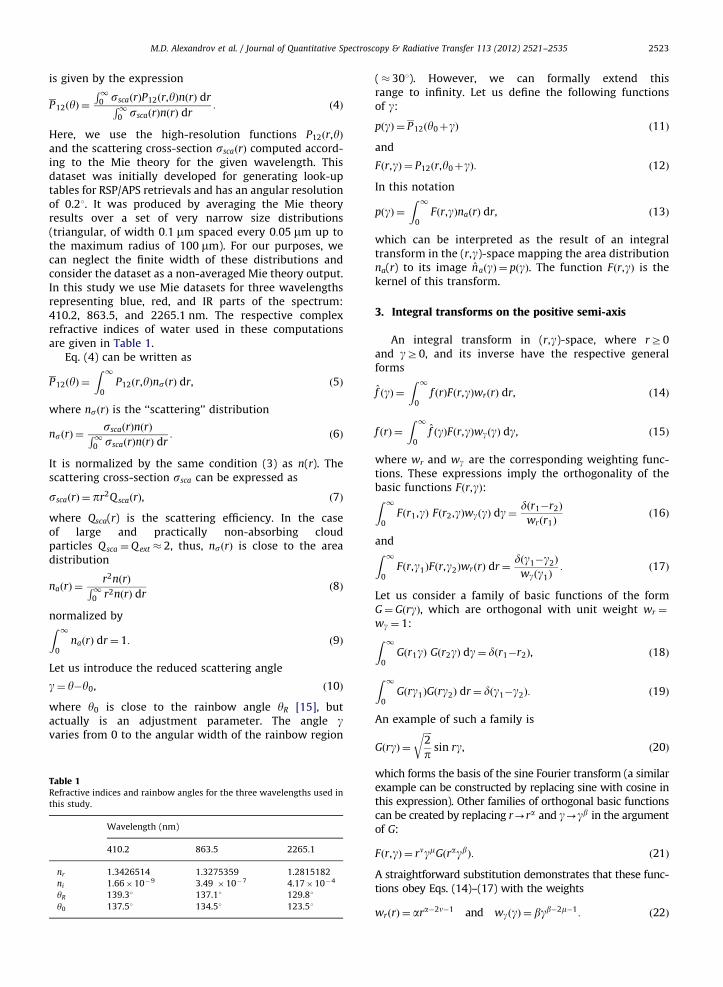
Fig. 1. Examples of polarized reflectances in the rainbow scattering

angle range. These radiative transfer simulations were made for realistic

cloud droplet size distributions with reff ¼ 7:5 mm (top) and 17:5 mm

(bottom). In both cases the gamma distribution model was used

with veff ¼ 0:01, 0.1, and 0.2, and the cloud optical depth was assumed

to be 5.

M.D. Alexandrov et al. / Journal of Quantitative Spectroscopy & Radiative Transfer 113 (2012) 2521–25352522

scattering of light by cloud particles. To account for thesmall contributions from all other factors (multiple scat-tering, Rayleigh scattering, aerosol extinction, groundsurface reflectance for thin clouds, as well as effectscaused by rotation to the scattering plane in Eq. (1)), themeasured polarized reflectance was fit by the expressionof the form

RpðyÞ ¼ A � PðMieÞ12 ½y;nðrÞ�þB � yþC, ð2Þ

where y is the scattering angle, n(r) is the cloud dropletsize distribution parameterized by its effective radius reff

and variance veff (the gamma distribution shape isassumed), while A, B, and C are the empirical fittingparameters (the linear term in y can be replaced with aRayleigh-like term � cos2 y [1]). The phase matrix ele-ments PðMieÞ

12 are computed using the Mie theory for a gridof reff and veff values. Alexandrov et al. [1] demonstratedthat this retrieval approach, while being very accurate,has a disadvantage associated with the necessity ofselecting an a priori functional shape of the droplet sizedistribution. If this shape is assumed to be monomodal,while the retrieval algorithm is applied to the data from a

cloud with a bimodal droplet distribution (e.g., includingdrizzle droplets), the retrieved effective size will be biasedtoward that of the dominant mode (this is a commonfeature of all least square fit retrievals).

In this study we present an alternative retrievalapproach based on our observation that the polarizedreflectances in the rainbow region taken as functions ofthe (reduced) scattering angle, while parameterized byparticle size, form a basis for an approximate integraltransform with certain similarities to the sine Fouriertransform on the positive semi-axis. This transformation,which we called the rainbow Fourier transform (RFT),turned out to have a simple inverse (as the ordinaryFourier transform). While the direct RFT acting from thespace of droplet size distributions (functions of theparticle radius r) into the space of rainbow polarizedreflectances (functions of the scattering angle y) is asimple integration used in direct modeling, its inverse,acting in the opposite direction, is a powerful retrievaltool for remote sensing of cloud microphysical properties.

We will describe the difference between the exact and‘‘approximate’’ transforms and show how to construct theaccurate inverse RFT on examples of droplet size distribu-tions of various shapes (such as rectangular and bimodalgamma distribution). We will also present some analyti-cal expressions derived from approximations to the Mietheory, which indirectly support our method. However,we currently have no theoretical proof of the RFT exis-tence based on the Mie theory, and our method is justifiedby empirical choices and is validated by numericalexperiments.

In practice, the proposed retrieval method is intendedto be used for analyses of measurements made by theResearch Scanning Polarimeter (RSP) [7–13]. This instru-ment is an airborne prototype for the satellite AerosolPolarimetery Sensor (APS), which was built as partof the NASA Glory Mission [14]. The RSP measures the I,Q, and U components of the Stokes vector in nine spectralchannels with center wavelengths of 410, 470, 555, 670,865, 960, 1590, 1880 and 2250 nm. It is a push-broomsensor scanning along the aircraft track within 7601 fromnadir (starting at forward direction) and making samplesat 0.81 intervals. Thus, each scan consists of about 150instantaneous measurements. The data from the actualRSP scans is then aggregated into ‘‘virtual’’ scans, eachconsisting of all reflectances (at a variety of scatteringangles) from a single point on the ground or at thecloud top. In recent years the RSP has been deployedonboard different aircrafts during a number of fieldcampaigns, making measurements for a vast variety ofcloud scenes.

2. Computation of the phase matrix element P12 for apolydisperse cloud

The averaged phase matrix element P12ðyÞ for a dropletsize distribution n(r), normalized by the conditionZ 1

0nðrÞ dr¼ 1 ð3Þ

M.D. Alexandrov et al. / Journal of Quantitative Spectroscopy & Radiative Transfer 113 (2012) 2521–2535 2523

is given by the expression

P12ðyÞ ¼R1

0 sscaðrÞP12ðr,yÞnðrÞ drR10 sscaðrÞnðrÞ dr

: ð4Þ

Here, we use the high-resolution functions P12ðr,yÞand the scattering cross-section sscaðrÞ computed accord-ing to the Mie theory for the given wavelength. Thisdataset was initially developed for generating look-uptables for RSP/APS retrievals and has an angular resolutionof 0.21. It was produced by averaging the Mie theoryresults over a set of very narrow size distributions(triangular, of width 0:1 mm spaced every 0:05 mm up tothe maximum radius of 100 mm). For our purposes, wecan neglect the finite width of these distributions andconsider the dataset as a non-averaged Mie theory output.In this study we use Mie datasets for three wavelengthsrepresenting blue, red, and IR parts of the spectrum:410.2, 863.5, and 2265.1 nm. The respective complexrefractive indices of water used in these computationsare given in Table 1.

Eq. (4) can be written as

P12ðyÞ ¼Z 1

0P12ðr,yÞnsðrÞ dr, ð5Þ

where nsðrÞ is the ‘‘scattering’’ distribution

nsðrÞ ¼sscaðrÞnðrÞR1

0 sscaðrÞnðrÞ dr: ð6Þ

It is normalized by the same condition (3) as n(r). Thescattering cross-section ssca can be expressed as

sscaðrÞ ¼ pr2QscaðrÞ, ð7Þ

where Qsca(r) is the scattering efficiency. In the caseof large and practically non-absorbing cloudparticles Qsca ¼Qext � 2, thus, nsðrÞ is close to the areadistribution

naðrÞ ¼r2nðrÞR1

0 r2nðrÞ drð8Þ

normalized byZ 10

naðrÞ dr¼ 1: ð9Þ

Let us introduce the reduced scattering angle

g¼ y�y0, ð10Þ

where y0 is close to the rainbow angle yR [15], butactually is an adjustment parameter. The angle gvaries from 0 to the angular width of the rainbow region

Table 1Refractive indices and rainbow angles for the three wavelengths used in

this study.

Wavelength (nm)

410.2 863.5 2265.1

nr 1.3426514 1.3275359 1.2815182

ni 1.66�10�9 3.49 �10�7 4.17�10�4

yR 139.31 137.11 129.81

y0 137.51 134.51 123.51

(� 301). However, we can formally extend thisrange to infinity. Let us define the following functionsof g:

pðgÞ ¼ P12ðy0þgÞ ð11Þ

and

Fðr,gÞ ¼ P12ðr,y0þgÞ: ð12Þ

In this notation

pðgÞ ¼Z 1

0Fðr,gÞnaðrÞ dr, ð13Þ

which can be interpreted as the result of an integraltransform in the (r,g)-space mapping the area distributionna(r) to its image naðgÞ ¼ pðgÞ. The function Fðr,gÞ is thekernel of this transform.

3. Integral transforms on the positive semi-axis

An integral transform in (r,g)-space, where rZ0and gZ0, and its inverse have the respective generalforms

f ðgÞ ¼Z 1

0f ðrÞFðr,gÞwrðrÞ dr, ð14Þ

f ðrÞ ¼

Z 10

f ðgÞFðr,gÞwgðgÞ dg, ð15Þ

where wr and wg are the corresponding weighting func-tions. These expressions imply the orthogonality of thebasic functions Fðr,gÞ:Z 1

0Fðr1,gÞ Fðr2,gÞwgðgÞ dg¼

dðr1�r2Þ

wrðr1Þð16Þ

andZ 10

Fðr,g1ÞFðr,g2ÞwrðrÞ dr¼dðg1�g2Þ

wgðg1Þ: ð17Þ

Let us consider a family of basic functions of the formG¼ GðrgÞ, which are orthogonal with unit weight wr ¼

wg ¼ 1:Z 10

Gðr1gÞ Gðr2gÞ dg¼ dðr1�r2Þ, ð18Þ

Z 10

Gðrg1ÞGðrg2Þ dr¼ dðg1�g2Þ: ð19Þ

An example of such a family is

GðrgÞ ¼ffiffiffiffi2

p

rsin rg, ð20Þ

which forms the basis of the sine Fourier transform (a similarexample can be constructed by replacing sine with cosine inthis expression). Other families of orthogonal basic functionscan be created by replacing r-ra and g-gb in the argumentof G:

Fðr,gÞ ¼ rngmGðragbÞ: ð21Þ

A straightforward substitution demonstrates that these func-tions obey Eqs. (14)–(17) with the weights

wrðrÞ ¼ ara�2n�1 and wgðgÞ ¼ bgb�2m�1: ð22Þ


4. Analytical approximations of P12

The amplitude scattering matrix (cf. [16]) relatesthe components of the incident electric field (propagatingin the positive z-direction) to that of the scattered radia-tion:

Esr

Eis

!¼

expð�ikRþ ikzÞ

ikR

S1 S4

S3 S2

!Ei

r

Eil

!: ð23Þ

Here, R is the distance from the particle (in the far-field),k¼ 2p=l is the wave number (l is the light wavelength),the indices r and l represent the components of E in anytwo mutually orthogonal directions. In the case of sphe-rical particles, the amplitude scattering matrix is diag-onal: S3 ¼ S4 ¼ 0. The Stokes vectors I¼ fI,Q ,U,Vg of theincident and scattered radiation are related by

I¼ssca

4pR2PI0, ð24Þ

where P is the 4�4 phase matrix. The element P12

determining polarized reflectance is expressed in termsof the amplitude scattering matrix elements as

P12 ¼2p

k2ssca

ð9S192�9S29

2Þ: ð25Þ

An idea of the functional dependence of P12 on the sizeparameter

b¼ kr¼2pr

lor k¼ 2b ð26Þ

(r is the spherical particle radius) and on the reducedscattering angle in the rainbow region E¼ y�yR (here yR isthe wavelength-dependent rainbow angle, see Table 1)can be obtained from the Airy approximation [15].This analytical approximation is formally valid forvery large size parameters b\5000 and very smallreduced angles Er0:51; however, as we show below, itcan lead to an approximate formula for P12 which isaccurate in a wider parameter range. The expression forthe amplitude scattering matrix elements in the Airyapproximation is

Sj ��2eijffiffiffiffipp

nujffiffiffiffiffiffiffiffiffiffiffisin yp k7=6Aið�0:369k2=3EÞ ð27Þ

j¼1, 2. Here, n is the real part of the refractive index ofwater, u1 ¼ 0:0381, u2 ¼ 0:00786, and eij is a phase factorirrelevant for absolute value computation. SubstitutingEq. (27) into Eq. (25) yields

P12 �0:04psin y

k1=3Ai2½�0:369k2=3E�: ð28Þ

The functions Ai2ðzÞ do not obey orthonormality relations

suitable for our purposes (cf. [17]), so we need to usefurther approximations. We use the fact that the Airyfunction Ai(z) is close to its asymptotic approximation[18] for a large negative argument

Aið�zÞ �z�1=4ffiffiffiffi

pp sin

2

3z3=2þ

p4

� �ð29Þ

even if the argument value is moderate. This leads to

Ai2ð�zÞ �

z�1=2

2p 1þsin4

3z3=2

� �� ð30Þ

and to another approximate formula for P12:

P12 �0:033

sin yE1=2½1þsinð0:3kE3=2Þ�: ð31Þ

As mentioned above, the Airy approximation (28) isformally valid only in the very close vicinity of yR:E5k�1=3

51, that is a few degrees. While Fig. 2 (top)demonstrates precisely this, it also shows that the exactMie function and the Airy approximation exhibit certainsimilarity within the entire rainbow range (1351–1651). Itis also seen in this plot that Ai2(x) in Eq. (28) is veryclosely approximated by its large-argument asymptoticsleading to Eq. (31). The exception is only for its firstquarter-period, while some deviations at substantiallylarger arguments simply indicate the need for a moreprecise asymptotic formula [18]. Based on Eq. (31) thefollowing analytical approximation for P12 can be intro-duced:

P12 ��0:035

E3=4sinð0:358kE1:605Þþ0:1E�0:05: ð32Þ

Its plot is shown in comparison with the exact curve inFig. 2 (bottom). Note that we are not looking for a highprecision approximation here, but only for an adequateanalytical expression to be used for educated guess of theintegral transform weights.

5. Definition of RFT

We can take the functional form of the first term in Eq.(32) as a proxy for the integral transform kernel (12):

Fðr,gÞ � g�3=4 sinðrg3=2Þ: ð33Þ

Here, g replaces E, giving us the freedom to choose y0

different from yR, and the particle radius r replaces thesize parameter k. We omit all constant factors for clarityand use 1:605� 3=2 (which makes a rather small phasechange in Eq. (32)). This expression coincides with Eq.(21), where the function GðxÞpsin x (Eq. (20)), and

a¼ 1, b¼ 32 , n¼ 0, m¼�3

4: ð34Þ

Thus, according to Eq. (22) the corresponding weightingfunctions are

wg ¼ g2 and wr ¼ 1: ð35Þ

This allows us to formally define the rainbow Fouriertransform (RFT) of the area size distribution na(r) as

naðgÞ ¼Z 1

0naðrÞFðr,gÞ dr ð36Þ

and its inverse

n0aðrÞ ¼

Z gmax

0naðgÞFðr,gÞg2 dg, ð37Þ

where the integration is performed within the rainbowregion (gmax � 301), and we use the exact kernels Fðr,gÞderived from the Mie theory (Eq. (12)) rather than theirapproximations. It appears that these functions are not

0 5 10 15 20 25 30-0.8

-0.6

-0.4

-0.2

0.0

0.2

0.4

MA

TRIX

ELE

ME

NT

P

0 5 10 15 20 25 30-0.8

-0.6

-0.4

-0.2

0.0

0.2

0.4

MA

TRIX

ELE

ME

NT

P

Fig. 2. Exact (derived from the Mie theory, red) and approximate dependences of the phase matrix element P12 on the reduced scattering angle E¼ y�yR.

Top: comparison with the Airy approximation Eq. (28) (dark blue) and the asymptotic formula Eq. (31)) (light blue). Bottom: Comparison with the

approximation of Eq. (32) (green). All computations were made for the size parameter b¼ 655, a 863 nm wavelength, and yR ¼ 1371. (For interpretation

of the references to color in this figure legend, the reader is referred to the web version of this article.)


precisely orthogonal, so the loop-transform (direct fol-lowed by inverse) is not an identity operator. This meansthat n0aana, but rather

n0aðrÞ � C1 � naðrÞþC2þnoise, ð38Þ

where C1 and C2 are constants, while ‘‘noise’’ stands forartifacts to be addressed in the next section.

The choice of the wavelength-dependent angle y0 ismade by keeping n0aðrÞ constant, where naðrÞ ¼ 0. If y0 istoo small, the bottom-line of n0aðrÞ tends to be convex(having maximum around 50 mm), while if y0 is too high,the bottom-line is concave. The values of y0 determined inthis way are summarized in Table 1 with the correspond-ing rainbow angles shown for comparison. The values ofy0 appear to be 2–61 lower than the corresponding anglesyR. Fig. 3 presents examples of RFT’s base functions (12)vs. the reduced angle g for 410, 863, and 2265 nmwavelengths. These plots show that at y¼ y0 (g¼ 0) thebase functions are close to 0, while yR is in the middle oftheir first half-period (as it is in the Airy approximation[15]). It is also clear from these plots that the curvescorresponding to the 410 and 863 nm wavelengths have a

more regular structure than that at 2265 nm. This may becaused by stronger absorption of water at the latterwavelength (see Table 1). Unfortunately, this lack ofstructure impairs the retrievals significantly, hence wewill present the results only for 410 and 863 nmwavelengths.

Fig. 4 shows the results of application of the loop-transform to two area size distributions na(r) of differentfunctional shapes: a bimodal gamma distribution [16] anda rectangular distribution (which is constant over aselected interval, and zero otherwise). The value of theconstant C2 in Eq. (38) is determined from the large-droplet range r� 902100 mm, where na(r) is assumed tobe zero. This value is subtracted from the retrieved n0aðrÞ,after which the constant C1 is supposed to be determinedfrom normalization condition Eq. (9). However, for ourtests, when the initial na(r) is known, we simply scale thereturned distribution so it has the same maximum valueas the initial one (in the case of the rectangular distribu-tion the median over the distribution top is taken insteadof the absolute maximum). The initial distributions na(r)are over-plotted (in black) for comparison. We use the

0 5 10 15 20 25 30-1.0

-0.8

-0.6

-0.4

-0.2

0.0

0.2

MA

TRIX

ELE

ME

NT

P

0 10 20 30-0.8

-0.6

-0.4

-0.2

0.0

0.2

MA

TRIX

ELE

ME

NT

P

0 10 20 30 40-0.3

-0.2

-0.1

0.0

0.1

STO

KE

S P

AR

AM

ETE

R P

Fig. 3. Examples of RFT’s basis functions Fðr,gÞ vs. the reduced angle gfor 10 and 100 mm droplet radii and different wavelengths: 410 nm

(top), 863 nm (middle), and 2265 nm (bottom).


metric [19]

D¼ 12

Z rmax

09n00aðrÞ�naðrÞ9 dr ð39Þ

to quantify how close the retrieved distribution is to theinitial one. Here n00aðrÞ denotes the loop-RFT result ofEq. (38) after the correction for the constants C1 and C2

described above. If both distributions n00aðrÞ and na(r) are

normalized to unity according to Eq. (9), this metricrepresents the fraction of the droplet ensemble that is‘‘misplaced’’ in the retrieved n00aðrÞ relative to the initialdistribution na(r). D¼ 0 would indicate that n00aðrÞ � naðrÞ,while D¼ 1 corresponds to the case when n00aðrÞ and na(r)do not have common support. In practice, normalizationof n00aðrÞ can be affected by retrieval errors, causing D toexceed 1. However, we still regard this metric as anadequate measure of the retrieval accuracy, which isconveniently expressed in per cent. We consider theaccuracy to be good if Dt10%.

6. Correction for weak orthogonality artifacts

While the loop-transform results presented in Fig. 4show generally good resemblance to the initial sizedistributions, some significant artifacts still contaminatethe retrievals causing large values of D� 30%. We assumethat these artifacts are caused mainly by the imperfectorthogonality of the RFT basis functions Fðr,gÞ. We mod-eled the effects of the weak orthogonality analytically (seeAppendix A) assuming that our basis functions can berepresented in the form

Fðr,gÞ ¼ cHðr,gÞþgðr,gÞ, ð40Þ

where c is a constant, Hðr,gÞ do satisfy appropriateorthogonality conditions, while gðr,gÞ is an additionalterm depending mainly on g and only weakly on r (notethat we do not know anything more specific about thesecomponents). Computations presented in Appendix Ashow that these assumptions lead to the expression forthe loop-transform result similar to Eq. (38)

n0aðrÞ ¼ c2naðrÞþZðrÞ, ð41Þ

where the correction function Z responsible for ‘‘noise’’can be represented as

ZðrÞ ¼ ZuðrÞþZsðrÞþZgðrÞþCZ: ð42Þ

Here, ZuðrÞ is a universal (independent of the size distributionna(r)) correction function, CZ is a (distribution-dependent)constant, while ZsðrÞ and ZgðrÞ are distribution-dependentcorrections, which, however, are substantially smaller inmagnitude than ZuðrÞ. The function ZsðrÞ has a rapidlyoscillating structure and can be represented in the form

ZsðrÞ ¼ B1s1ðrÞþB0s0ðrÞ, ð43Þ

where B0 and B1 are (distribution-dependent) constants,while

s0ðrÞ ¼

Z gmax

0Fðr,gÞg2 dg ð44Þ

and

s1ðrÞ ¼

Z gmax

0gFðr,gÞg2 dg ð45Þ

are universal functions. The function ZgðrÞ is assumed to beslowly varying, while its specific structure is unknown.

Based on this model consideration and results ofnumerical tests, we can design a correction procedureallowing the separation and removal of the artifactsfrom n0aðrÞ, and the restoration of the original distributionna(r). We should note that, as mentioned above, the total

0 20 40 60 80 100PARTICLE RADIUS, μm

-0.02

0.00

0.02

0.04

0.06

FRE

QU

EN

CY

of O

CC

UR

RE

NC

E


-0.01

0.00

0.01

0.02

0.03

0.04

FRE

QU

EN

CY

of O

CC

UR

RE

NC

E


-0.02

0.00

0.02

0.04

0.06

FRE

QU

EN

CY

of O

CC

UR

RE

NC

E


-0.01

0.00

0.01

0.02

0.03

0.04

FRE

QU

EN

CY

of O

CC

UR

RE

NC

E

Fig. 4. Examples of RFT loop-transforms (green) of two model area size distributions (plotted in black for comparison). Left: bimodal gamma distribution

with equally (50% each) weighted modes having 40 and 70 mm effective radius and the same effective variance of 0.01. Right: rectangular distribution

which is constant between particle radii of 30 and 70 mm, and zero otherwise. The plots correspond to 410 (top) and 863 nm (bottom) wavelengths. (For

interpretation of the references to color in this figure legend, the reader is referred to the web version of this article.)


constant contribution to n0aðrÞ can easily be determinedfrom its value at very large r and subtracted. Thus, it issufficient for us to determine all the r-dependent artifactfunctions up to a constant (even if it is distribution-dependent), so we will use the terms ‘‘distribution-inde-pendent’’ and ‘‘universal’’ neglecting such additive con-stant dependence. Our numerical tests confirm that thecorrection function ZðrÞ is mostly universal, i.e., its shapeonly weakly depends on the particular area distributionna(r). Thus, as the first step of the correction procedure wecompute ZðrÞ using a default size distribution nd(r). It isconvenient for this purpose to use the constant sizedistribution ndðrÞ ¼ 1=rmax, where rmax ¼ 100 mm is theupper limit of particle radius in our Mie theory dataset(ndðr4rmaxÞ ¼ 0 is assumed). Thus, we define

ZdðrÞ ¼ n0dðrÞ ð46Þ

i.e., the result of the loop-RFT applied to nd(r) (subtractionof the first term from Eq. (41) is not necessary, since it isconstant). Plots of the resulting correction functions areshown in Fig. 5 (left) for 410 and 863 nm wavelengths(these functions are (arbitrarily) normalized to satisfy

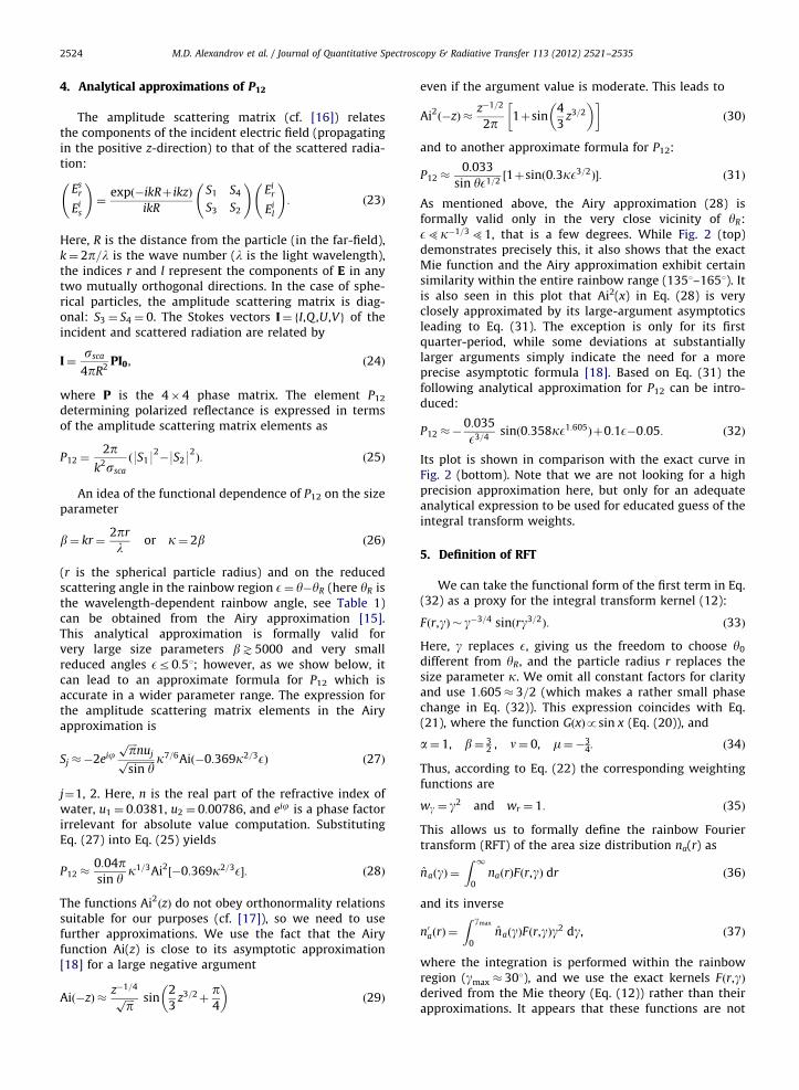
ZdðrmaxÞ ¼ 0). The first step of our correction procedureis simply the subtraction of the pre-computed functionZdðrÞ from the initial loop-transform result n0aðrÞ. Theresults of this operation (complemented by a moving-window smoothing) applied to the distributions fromFig. 4 are shown in Fig. 6 demonstrating improvementin retrieval accuracy from D� 30% to 5–6%. Analyticallythese results can be represented in the form

n00aðrÞ ¼ n0aðrÞ�ZdðrÞ

¼ c2naðrÞþDZsðrÞþDZgðrÞ ð47Þ

(where we omit constant terms), since the universal ZuðrÞ

cancels from the difference. The oscillatory artifacts inFig. 6 are consistent with the shape of DZsðrÞ, which is alinear combination of s0ðrÞ and s1ðrÞ, both exhibiting rapidoscillations with a frequency � gmax, as can be seen inFig. 5 (right). Note that these oscillatory patterns have adifferent shape than the artifacts caused by the truncationof the integration range (ringing effects, Gibbs ripples),whose amplitude decreases with distance from the dis-tribution maximum. In order to remove these artifacts, we


-0.10

0.00

0.10

0.20

CO

RR

EC

TIO

N F

UN

CTI

ON

410 nm


-0.15

-0.10

-0.05

-0.00

0.05

CO

RR

EC

TIO

N F

UN

CTI

ON

S

410 nm


-0.4

-0.2

0.0

0.2

0.4

CO

RR

EC

TIO

N F

UN

CTI

ON

863 nm


-0.3

-0.2

-0.1

-0.0

0.1

CO

RR

EC

TIO

N F

UN

CTI

ON

S

863 nm

Fig. 5. Plots of the universal correction functions for 410 nm (top) and 863 nm (bottom) wavelengths. Left: ZdðrÞ (green), black curves depict moving

averages to better show the oscillating structure. Right: s0ðrÞ (red) and s1ðrÞ, scaled to magnitude of s0 (blue). (For interpretation of the references to color

in this figure legend, the reader is referred to the web version of this article.)


numerically compute the functions s0ðrÞ and s1ðrÞ accord-ing to Eqs. (44) and (45), and then perform a multivariatelinear regression on n00aðrÞ, as the second step of our clean-up procedure. This regression also includes an exponen-tial function exp(�0.07r) that improves the retrieveddistribution shape at small r (probably, compensatingfor the unknown ZgðrÞ), and uses weighting functionr�5=2 (both are empirical guesses). Note that while s0ðrÞ

and s1ðrÞ look almost identical (after rescaling) in Fig. 5(right), they have enough differences in the small particlesize range, so both of them should be used in theregression. The resulting size distribution is the residueof this regression. The examples presented in Fig. 7demonstrate a successful removal of the oscillating arti-facts present in Fig. 6 and further accuracy improvementto D� 324%. The remaining small differences with theinitial size distributions can be attributed to the unknownsmooth component ZgðrÞ, which cannot be objectivelyseparated from the distribution shape.

Note that since ZdðrÞ exhibits some slope, the finaladjustment of the lower integration limit y0 should be madebased on the condition that the retrieved size distribution hasa constant bottom-line after Zd is subtracted.

7. Retrievals in the presence of multiple scattering

While polarized reflectance emerging from a cloud islargely dominated by single scattering by cloud droplets,it also includes a residual contribution from multiplescattering and other factors (Rayleigh scattering, aerosolextinction, etc.). This contribution can be well approxi-mated by a term linear in scattering angle plus a constant[3,4,1], as shown in Eq. (2). The additional term

sðgÞ ¼ BgþC ð48Þ

in naðgÞ generates contamination of n0aðrÞ having the form

sðrÞ ¼ Bs1ðrÞþCs0ðrÞ, ð49Þ

where s0ðrÞ and s1ðrÞ are defined by Eqs. (44) and (45). Theeffect of such contamination generated by sðgÞ ¼ 0:1gþ0:2on the retrievals from Fig. 6 is shown in Fig. 8. Obviously,this contamination has the same shape as ZsðrÞ describedin the previous section (Eq. (43)), and is thereforeremoved during the second step of our correction proce-dure leading to the same final results presented in Fig. 7.Thus, this term alone does not present an additionalchallenge to the retrieval method. However, the retrievals


-0.02

0.00

0.02

0.04

0.06

FRE

QU

EN

CY

of O

CC

UR

RE

NC

E


-0.01

0.00

0.01

0.02

0.03

0.04

FRE

QU

EN

CY

of O

CC

UR

RE

NC

E


-0.02

0.00

0.02

0.04

0.06

FRE

QU

EN

CY

of O

CC

UR

RE

NC

E


-0.01

0.00

0.01

0.02

0.03

0.04

FRE

QU

EN

CY

of O

CC

UR

RE

NC

E

Fig. 6. Same as in Fig. 4, but with the corresponding correction functions ZdðrÞ [Fig. 5 (left)] subtracted. In addition to that a moving (11 points¼0.5 nm)

window smoothing was applied. The plots correspond to 410 (top) and 863 nm (bottom) wavelengths.


from the polarized reflectances having the form of Eq. (2)are complicated by the presence of the unknown coeffi-cient A. Indeed, while naðgÞ is now scaled, the defaultloop-RFT result ZdðrÞ should be scaled accordingly beforethe subtraction. This suggests that we should combine thefirst and second steps of the correction method describedabove into a single multivariate regression in threecomponents: ZdðrÞ, s0ðrÞ, and s1ðrÞ (with a possibleadditional smooth component). Generally speaking, anincrease in the number of regression components couldmake it less stable (due to increasing possibility of trade-offs between these components). However, in our case theresults of the combined regression correction procedureare practically indistinguishable from those of the originalmethod.

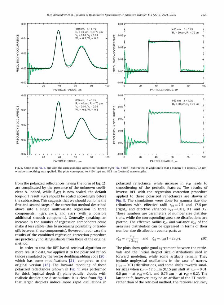
In order to test the RFT-based retrieval algorithm onmore realistic data, we applied it to the polarized reflec-tances simulated by the vector doubling/adding code [20],which has some modifications [21] compared to theoriginal version [16]. The forward modeling of thesepolarized reflectances (shown in Fig. 1) was performedfor thick (optical depth 5) plane-parallel clouds withrealistic droplet size distributions. It is clear from Fig. 1that larger droplets induce more rapid oscillations in

polarized reflectance, while increase in veff leads tosmoothening of the periodic features. The results ofinverse RFT with the regression correction procedureapplied to these polarized reflectances are shown inFig. 9. The simulations were done for gamma size dis-tributions with effective radii reff ¼ 7:5 and 17:5 mm(right), and effective variances veff ¼ 0:01, 0.1, and 0.2.These numbers are parameters of number size distribu-tions, while the corresponding area size distributions areplotted. The effective radius r0eff and variance v0eff of thearea size distribution can be expressed in terms of theirnumber size distribution counterparts as

v0eff ¼veff

1þ2veffand r0eff ¼ reff ð1þ2veff Þ: ð50Þ

The plots show quite good agreement between the retrie-vals and the initial droplet size distributions used inforward modeling, while some artifacts remain. Theyinclude unphysical oscillations in the case of narrow(veff ¼ 0:01) distributions, and some shifts towards smal-ler sizes when reff ¼ 17:5 mm (0:15 mm shift at veff ¼ 0:01,0:5 mm – at veff ¼ 0:1, and 0:75 mm – at veff ¼ 0:2). Thelatter shift, however, may be an artifact of the RT model,rather than of the retrieval method. The retrieval accuracy


-0.02

0.00

0.02

0.04

0.06

FRE

QU

EN

CY

of O

CC

UR

RE

NC

E


-0.01

0.00

0.01

0.02

0.03

0.04

FRE

QU

EN

CY

of O

CC

UR

RE

NC

E


-0.02

0.00

0.02

0.04

0.06

FRE

QU

EN

CY

of O

CC

UR

RE

NC

E


-0.01

0.00

0.01

0.02

0.03

0.04

FRE

QU

EN

CY

of O

CC

UR

RE

NC

E

Fig. 7. Same as in Fig. 6, but after application of multivariate regression in s0ðrÞ and s1ðrÞ from Fig. 5 (right), which removes the oscillating artifacts.


appears to be better for larger values of reff and/or veff ,since the RFT artifacts are stronger in the small-radiusrange. In the worst considered case of reff ¼ 7:5 mm andveff ¼ 0:01, the error is particularly large (D¼ 50%), whilefor veff Z0:1 it is substantially smaller (Dr14%). In thecase of reff ¼ 17:5 mm, the accuracy is even better(D� 6210%).

8. Practical application issues

In this paper we focus on the introduction of a newretrieval algorithm and description of its mathematicalbasis. Thus, we will only briefly address the issues ofapplication of RFT to real data (such as measurements bythe RSP), leaving detailed sensitivity studies to futurepublications. Some of these sensitivities, which are com-mon to all rainbow-based retrieval techniques aredescribed in detail in another article [1]. They includethe effects of rotation to the principal plane, uncertaintiesin aircraft attitude (pitch and crab angles), multiplescattering contribution (including 3D effects), and thepresence of aerosol layer above clouds.

The issues specific to RFT are related to angular range andresolution requirements for the measurements, as well as theinformation content of the retrieved droplet distribution

shape. Our preliminary tests on simulated and real RSP datashowed that availability of measurements in full rainbowscattering angle range is essential for applicability of RFT. Forexample, reduction of the upper limit of this range from 1651to 1551 significantly impairs the retrievals. This is under-standable, since such reduction affects orthogonality of theRFT’s basis functions. Degradation of measurement resolutionis expected to primarily affect high-frequency components ofthe angular spectrum, which correspond, as we can see fromFig. 1, to large particles and/or narrow size distributions (aswell as to sharp features in the size distribution shape). Adetailed quantitative study of these effects is yet to be done.The results of our preliminary tests show that the effect of afactor of four resolution reduction (from the model’s 0.21 tothe RSP’s 0.81) is practically indistinguishable for area sizedistributions having monomodal gamma shape with reff upto 70 mm (it causes only a few per cent increase in D). RFTwith 1.61 resolution (factor of 8 degradation) works fine forrelatively wide distributions (veff ¼ 0:120:2), while in thecase of a narrow distribution (veff ¼ 0:01) its performanceworsens. However, even in the latter case it still canadequately resolve the distribution maximum for reff valuesup to 40 mm (but with increase in D from 7% to 35%). Theseobservations suggest that RFT should not be expected toperform well on datasets with angular resolution worse than


-0.02

0.00

0.02

0.04

0.06

FRE

QU

EN

CY

of O

CC

UR

RE

NC

E


-0.01

0.00

0.01

0.02

0.03

0.04

FRE

QU

EN

CY

of O

CC

UR

RE

NC

E


-0.02

0.00

0.02

0.04

0.06

FRE

QU

EN

CY

of O

CC

UR

RE

NC

E


-0.01

0.00

0.01

0.02

0.03

0.04

FRE

QU

EN

CY

of O

CC

UR

RE

NC

E

Fig. 8. Same as in Fig. 6, but with the effects of contamination of naðgÞ with sðgÞ ¼ 0:1gþ0:2.


21, since the droplet size distributions at the cloud top (whichdominate the airborne polarimetric measurements) are typi-cally narrow.

Unlike fitting techniques, integral transforms (includingthe RFT) cannot be forced to constrain their results to acertain family of functions, such as statistical distributions(i.e., positive normalized functions). This means that whileRFT is expected to adequately determine the functional shapeof a droplet size distribution, presence of noise and negativevalues may impact the integration of this distribution overthe size range, leading to inaccurate computation of its normand moments. In the case of a generic distribution shape, thisproblem needs further study. However, when the sizedistribution is expected to have gamma distribution shape,its effective radius and variance can be derived withoutintegration. Fortunately, this is the case for the droplet sizedistributions at the cloud top, which are important forairborne polarimetric measurements. Their tendency to havegamma distribution shape was confirmed by both theoreticalmodel [22,23], and airborne in situ measurements (cf. [24]).Our own results of application of RFT to real RSP data alsosupport this assertion. While a direct functional fitting can beused in order to derive the distribution parameters in thiscase, we propose another, computationally simpler, approachbased on variation of the distribution in the vicinity of its

maximum (which is usually free from RFT-generated noise).This approach uses three metrics of the retrieved distributionshape n(r): position of the distribution maximum (moderadius)

rmax ¼ reff ð1�3veff Þ ð51Þ

and the two ratios

r¼ r

rmaxand R¼

nðrÞ

nðrmaxÞ: ð52Þ

Note that none of these metrics requires proper normal-ization of the retrieved distribution. Then, we derive veff , first,from the relation

ln R¼1

veff�3

� �½ln rþð1�rÞ� ð53Þ

for some fixed value of r and the corresponding value of R

(we found r¼ 0:8 to be optimal for r4rmax). After that wedetermine reff from Eq. (51). This method produces goodresults, when applied to the distributions from Fig. 9, espe-cially for veff ¼ 0:01, when the errors in reff and veff are lessthan 0:1mm and 0.01, respectively. For veff ¼ 0:1 and 0.2, thecorresponding errors are larger, but they are still less than0:5 mm in reff and 0.1 in veff .


-0.2

0.0

0.2

0.4

0.6

FRE

QU

EN

CY

of O

CC

UR

RE

NC

E


-0.05

0.00

0.05

0.10

0.15

0.20

0.25

0.30

FRE

QU

EN

CY

of O

CC

UR

RE

NC

E


-0.05

0.00

0.05

0.10

0.15

0.20

FRE

QU

EN

CY

of O

CC

UR

RE

NC

E


-0.02

0.00

0.02

0.04

0.06

0.08

0.10

FRE

QU

EN

CY

of O

CC

UR

RE

NC

E


-0.05

0.00

0.05

0.10

0.15

FRE

QU

EN

CY

of O

CC

UR

RE

NC

E


-0.02

0.00

0.02

0.04

0.06

0.08

FRE

QU

EN

CY

of O

CC

UR

RE

NC

E

Fig. 9. Results of the inverse RFT (with regression correction) applied to polarized reflectances simulated using a vector radiative transfer code

(accounting for multiple scattering contribution). The simulations were made for gamma size distributions with reff ¼ 7:5 (left) and 17:5 mm (right), and

veff ¼ 0:01, 0.1, and 0.2 (from top to bottom). Note that these numbers are parameters of the number size distributions, while the corresponding area size

distributions are plotted: the retrieved (green) and the original (black). (For interpretation of the references to color in this figure legend, the reader is

referred to the web version of this article.)


9. Conclusions

We described a new approach (the rainbow Fouriertransform) to the retrieval of cloud droplet size distribu-tions from polarized reflectances in the rainbow scatter-ing angle range (1351–1651), where they are dominated

by single scattering. This method is based on the observa-tion that these polarized reflectances computed usingthe Mie theory for a range of (monodisperse) particleradii as functions of reduced scattering angle g form aproxy basis of an integral transform (similar to the sineFourier transform or the Bessel transform on the positive


semi-axis). The direct transform applied to a given dropletsize distribution coincides with the computation of thecorresponding polarized reflectance. The inverse trans-form applied to this polarized reflectance as a function ofscattering angle yields a proxy of the original size dis-tribution. To obtain the distribution itself, a simpleregression-based correction procedure is applied, whichremoves retrieval artifacts from this proxy function. Ouranalytical modeling suggested that these artifacts arecaused by the lack of orthogonality of the RFT’s basefunctions. We demonstrated good performance of thedescribed technique using various sample droplet sizedistributions (bimodal gamma and rectangular) at 410and 863 nm wavelengths marking the boundaries of thevisible spectral range. We also showed using RT simula-tions that our approach works well in realistic situations,when the measurements are made in the presence ofmultiple scattering.

The main advantage of the RFT-based retrieval algo-rithm compared to the currently used fitting methods[3,4,1] is that this technique is non-parametric, i.e., it doesnot require any a priori knowledge of the droplet sizedistribution functional shape (including the number ofmodes). This also makes our algorithm computationallyfast, since its computations used for inversions are essen-tially the same as those used for the forward modeling.There is no fitting using look-up tables.

We expect that the method described has a potentialto detect drizzle in clouds along with the cloud dropletdistribution. However, successful use of the RFT-basedtechnique imposes certain requirements on the measure-ments, including high angular resolution (better than 21),wide angular range (close to the full rainbow range, whichcan be observed in solar principle plane measurements),and high measurement accuracy (low instrumentalnoise). This method will be applied to the RSP data froma number of field campaigns.

Acknowledgments

This basic research was funded by the NASA RadiationSciences Program managed by Hal Maring and by theNASA Glory Mission project.

Appendix A. Effects of weak orthogonality

Let us assume that the lack of orthogonality of the RFTbasis functions Fðr,gÞ is caused by an additive term gðr,gÞ,i.e., these functions can be represented in the form

Fðr,gÞ ¼ cHðr,gÞþgðr,gÞ, ðA:1Þ

where c is a constant, and Hðr,gÞ satisfy the orthogonalityconditions (16) and (17) with the weights from Eq. (35).Hðr,gÞ can be used as the kernel of another integraltransform

nHðgÞ ¼Z 1

0naðrÞHðr,gÞ dr, ðA:2Þ

which, unlike RFT, is exact, i.e.

naðrÞ ¼

Z gmax

0nHðgÞHðr,gÞg2 dg: ðA:3Þ

Here, we neglect the effect of finiteness of the integrationlimit gmax, which generally may cause artificial oscilla-tions (ringing artifacts, Gibbs ripples), since the latter donot show up in numerical tests. The result of the originalRFT (F-transform, Eq. (36)) can be expressed in terms ofthis H-transform as

nF ðgÞ ¼ cnHðgÞþgðgÞ, ðA:4Þ

where

gðgÞ ¼Z 1

0naðrÞgðr,gÞ dr: ðA:5Þ

Then, the result of the inverse RFT (Eq. (37)) can bewritten as

n0aðrÞ ¼

Z gmax

0½cnHðgÞþgðgÞ�Fðr,gÞg2 dg

¼ c2naðrÞþZðrÞ, ðA:6Þ

where

ZðrÞ ¼ Z0ðrÞþZ1ðrÞ ðA:7Þ

with

Z0ðrÞ ¼ c

Z gmax

0nHðgÞgðr,gÞg2 dg ðA:8Þ

and

Z1ðrÞ ¼

Z gmax

0g ðgÞFðr,gÞg2 dg ðA:9Þ

describe the non-orthogonality artifacts in the loop RFT.Using Eq. (A.2) and changing the integration order (weassume all the convergence properties necessary for this),Eq. (A.8) can be written as

Z0ðrÞ ¼ c

Z gmax

0g2 dg gðr,gÞ

Z 10

dr0naðr0ÞHðr0,gÞ

¼

Z 10

naðr0Þhðr,r0Þ dr0, ðA:10Þ

where

hðr,r0Þ ¼ c

Z gmax

0gðr,gÞHðr0,gÞg2 dg: ðA:11Þ

Similarly, Eq. (A.9) can be written in the following form,using Eq. (A.5):

Z1ðrÞ ¼ c

Z gmax

0g2 dg Fðr,gÞ

Z 10

dr0naðr0Þgðr0,gÞ

¼

Z 10

naðr0Þf ðr0,rÞ dr0, ðA:12Þ

where

f ðr,r0Þ ¼

Z gmax

0gðr,gÞFðr0,gÞg2 dg: ðA:13Þ

The function hðr,r0Þ in Eq. (A.10) can be expressed in termsof f ðr,r0Þ as

hðr,r0Þ ¼ f ðr,r0Þ�yðr,r0Þ, ðA:14Þ


where

yðr,r0Þ ¼

Z gmax

0gðr,gÞgðr0,gÞg2 dg ðA:15Þ

(obviously, y is symmetric: yðr,r0Þ ¼ yðr0,rÞ). In this nota-tion the expression for ZðrÞ has the following form:

ZðrÞ ¼Z 1

0naðr

0Þpðr,r0Þ dr0, ðA:16Þ

where

pðr,r0Þ ¼ f ðr,r0Þþ f ðr0,rÞ�yðr,r0Þ ðA:17Þ

is symmetric function: pðr,r0Þ ¼ pðr0,rÞ.Our numerical tests show that the shape of ZðrÞ is

almost independent of the size distribution na(r) (it may,however, include a distribution-dependent constant,which can always be removed by taking into account thatnaðrÞ ¼ 0 at very large r. As we show below, completedistribution-independence in the above sense is achievedif the additive term gðr,gÞ does not depend on particleradius: g ¼ g0ðgÞ. This allows us to consider the r-depen-dent part of the term g as a small perturbation

gðr,gÞ ¼ g0ðgÞþe g1ðr,gÞ, ðA:18Þ

where e is a small parameter. In this case

f ðr,r0Þ ¼ f 0ðr0Þþef 1ðr,r0Þ, ðA:19Þ

where

f 0ðr0Þ ¼

Z gmax

0g0ðgÞFðr0,gÞg2 dg ðA:20Þ

and

f 1ðr,r0Þ ¼

Z gmax

0g1ðr,gÞFðr0,gÞg2 dg: ðA:21Þ

In computation of yðr,r0Þ, we omit terms quadratic in eyðr,r0Þ ¼ y0þe½y1ðrÞþy1ðr

0Þ�, ðA:22Þ

where

y0 ¼

Z gmax

0g2

0ðgÞg2 dg ðA:23Þ

is a constant, and

y1ðrÞ ¼

Z gmax

0g0ðgÞg1ðr,gÞg2 dg: ðA:24Þ

Thus

pðr,r0Þ ¼ f 0ðrÞþ f 0ðr0Þþe½f 1ðr,r0Þþ f 1ðr

0,rÞ��y0�e½y1ðrÞþy1ðr0Þ�

ðA:25Þ

and

ZðrÞ ¼ ZuðrÞþZsðrÞþZgðrÞþCZ, ðA:26Þ

where

ZuðrÞ ¼ f 0ðrÞ�ey1ðrÞ ðA:27Þ

is a distribution-independent (universal) function

CZ ¼ f 0�y0�ey1 ðA:28Þ

is a constant (here the bar denotes an average with naðr0Þ),while the terms

ZsðrÞ ¼ eZ 1

0naðr

0Þf 1ðr0,rÞ dr0 ðA:29Þ

and

ZgðrÞ ¼ eZ 1

0naðr

0Þf 1ðr,r0Þ dr0 ðA:30Þ

are the functions of particle radius, which depend on thesize distribution shape. Note that these terms disappearwhen e¼ 0 (i.e., when g depends on g only), and ZðrÞbecomes universal (up to a constant). To understand thestructure of ZsðrÞ and ZgðrÞ, let us represent g1ðr,gÞ by itsTaylor’s series expansion in g

g1ðr,gÞ ¼X1

0

g1iðrÞgi, ðA:31Þ

which we assume to be uniformly convergent on thefinite interval ½0,gmax� for all r. Then

f 1ðr,r0Þ ¼X1

0

g1iðrÞsiðr0Þ, ðA:32Þ

where

siðrÞ ¼

Z gmax

0giFðr,gÞg2 dg: ðA:33Þ

Thus

ZsðrÞ ¼ eX1

0

g1isiðrÞ ðA:34Þ

and

ZgðrÞ ¼ eX1

0

g1iðrÞsi : ðA:35Þ

The functions si(r) show rapid oscillations with frequency� gmax. The plots of s0 and s1 are shown in Fig. 5 (right).On the other hand, g1iðrÞ are expected to be smooth slowlyvarying functions of r. This makes it difficult (if evenpossible) to separate them from the size distributionfeatures. Fortunately, they appear to be small in magni-tude. It appears from our numerical simulations that foran adequate fit of n0aðrÞ only first two terms in theexpansion of g1ðr,gÞ are needed for an adequate fit ofn0aðrÞ:

g1ðr,gÞ � g10ðrÞþg11ðrÞg: ðA:36Þ

This simplifies the expression for ZsðrÞ:

ZsðrÞ � e½g10s0ðrÞþg11s1ðrÞ�: ðA:37Þ

References

[1] Alexandrov MD, Cairns B, Emde C, Ackerman AS, van DiedenhovenB. Characterization of cloud droplet size distributions based onpolarized reflectance measurements by the research scanningpolarimeter: sensitivity study. Atmos Chem Phys; to be submitted.

[2] Mishchenko MI, Travis LD, Lacis AA. Multiple scattering of light byparticles: radiative transfer and coherent backscattering. Cam-bridge University Press; 2006.

[3] Breon FM, Goloub P. Cloud droplet effective radius from spacebornepolarization measurements. Geophys Res Lett 1998;25:1879–82.

[4] Breon FM, Doutriaux-Boucher M. A comparison of cloud dropletradii measured from space. IEEE Trans Geosci Remote Sensing2005;43:1796–805.

[5] Platnick S, Valero FPJ. A validation study of a satellite cloudretrieval during ASTEX. J Atmos Sci 1995;52:2985–3001.

[6] Coddington OM, Pilewskie P, Redemann J, Platnick S, Russell PB,Schmidt KS, et al. Examining the impact of overlying aerosols on


the retrieval of cloud optical properties from passive remotesensing. J Geophys Res 2010;115:D10211.

[7] Cairns B, Russell EE, Travis LD. Research scanning polarimeter:calibration and ground-based measurements. In: Proceedings ofSPIE, vol. 3754; 1999. p. 186–97.

[8] Cairns B, Waquet F, Knobelspiesse K, Chowdhary J, Deuze JL.Polarimetric remote sensing of aerosols over land surfaces. In:Kokhanovsky AA, Leeuw GD, editors. Satellite aerosol remotesensing over land. Springer; 2009. p. 295–325.

[9] Waquet F, Cairns B, Knobelspiesse K, Chowdhary J, Travis LD,Schmid B, et al. Polarimetric remote sensing of aerosols over land.J Geophys Res 2009;114:D01206.

[10] Chowdhary J, Cairns B, Mishchenko MI, Hobbs PV, Cota GF,Redemann J, et al. Retrieval of aerosol scattering and absorptionproperties from photopolarimetric observations over the oceanduring the CLAMS experiment. J Atmos Sci 2005;62:1093–117.

[11] Knobelspiesse KD, Cairns B, Schmid B, Roman MO, Schaaf CB.Surface BRDF estimation from an aircraft compared to MODIS andground estimates at the Southern Great Plains site. J Geophys Res2008;113:D20105.

[12] Knobelspiesse KD, Cairns B, Redemann J, Bergstrom RW, Stohl A.Simultaneous retrieval of aerosol and cloud properties during theMILAGRO field campaign. Atmos Chem Phys 2011;11:6245–63.

[13] Knobelspiesse KD, Cairns B, Ottaviani M, Ferrare R, Hair J, Hostetler C,et al. Combined retrievals of boreal forest fire aerosol properties witha polarimeter and lidar. Atmos Chem Phys 2011;11:7045–67.

[14] Mishchenko MI, Cairns B, Kopp G, Schueler CF, Fafaul BA, Hansen JE,et al. Accurate monitoring of terrestrial aerosols and total solar

irradiance: introducing the glory mission. Bull Am Meteorol Soc2007;88:677–91.

[15] Grandy WT. In: Scattering of waves from large spheres.CambridgeUniversity Press; 2000.

[16] Hansen JE, Travis LD. Light scattering in planetary atmospheres.Space Sci Rev 1974;16:527–610.

[17] Vallee O, Soares M. Airy functions and applications to physics.Imperial College Press; 2004.

[18] Abramowitz M, Stegun IA. Handbook of mathematical functions.Washington: National Bureau of Standards; 1964 [Reprinted byDover, New York, 1972].

[19] Alexandrov MD, Ackerman AS, Marshak A. Cellular statisticalmodels of broken cloud fields. Part II: comparison with a dynamicalmodel and statistics of diverse ensembles. J Atmos Sci 2010;67:2152–70.

[20] Cairns B, Carlson BE, Lacis AA, Russell EE. An analysis of ground-based polarimetric sky radiance measurements. In: Proceedings ofSPIE, vol. 3121; 1997. p. 382–93.

[21] de Haan JF, Bosma PB, Hovenier JW. The adding method formultiple scattering calculations of polarized light. Astron Astrophys1987;183:371–2.

[22] Khvorostyanov VI, Curry JA. Toward the theory of stochasticcondensation in clouds. Part II: analytical solutions of thegamma-distribution type. J Atmos Sci 1999;56:3997–4013.

[23] Khvorostyanov VI, Curry JA. Analytical solutions to the stochastickinetic equation for liquid and ice particle size spectra. Part I:small-size fraction. J Atmos Sci 2008;65:2025–43.

[24] Pruppacher HR, Klett JD. Microphysics of clouds and precipitation.Kluwer; 1997.

Contents lists available at SciVerse ScienceDirect Journal ...theory, which indirectly support our...

Documents

Transcript of Contents lists available at SciVerse ScienceDirect Journal ...theory, which indirectly support our...