Journal of International Money and Finance 29 (2010) 1369–1384

Contents lists available at ScienceDirect

Journal of International Moneyand Finance

journal homepage: www.elsevier .com/locate/ j imf

Cagan’s paradox and money demand in hyperinflation:Revisited at daily frequency

Zorica Mladenovi�c, Pavle Petrovi�c*

University of Belgrade, Economics Faculty, Kameni�cka 6, 11 000 Belgrade, Serbia

JELs classification:E 31E 41E 51

Keywords:HyperinflationMoney demandCagan’s paradoxDaily frequency

* Corresponding author. Tel.: þ381 63 434 103;E-mail address: pavlep@eunet.rs (P. Petrovi�c).

0261-5606/$ – see front matter � 2010 Elsevier Ltdoi:10.1016/j.jimonfin.2010.05.005

a b s t r a c t

Using daily data the Cagan money demand is estimated andaccepted for the most severe portion of Serbia’s 1992–1993hyperinflation, i.e. its last 6 months. An implication is that thepublic adjusted daily throughout this extreme period. Moreover,the obtained semi-elasticity estimates are by far lower than thosepreviously found using monthly data sets. Consequently, the dailyestimates reject the longstanding Cagan’s paradox, based onmonthly studies, by showing that the economy has been on thecorrect, increasing side of the Laffer curve almost through the endof hyperinflation. This strongly supports the view that hyperin-flation is triggered and driven all way through its end by thegovernment’s hunt for non-decreasing seigniorage. Daily adjust-ments of public in hyperinflation can account for the differencebetween the results obtained at daily and monthly frequencies,calling into question the latter. Some evidence is offered that thefindings of this paper may hold for other hyperinflations.

� 2010 Elsevier Ltd. All rights reserved.

1. Introduction

There has been a longstanding interest, initiated by Cagan (1956) in exploring money demand inhyperinflation, and most relevant studies have been done using monthly data. However, hyperinfla-tions are extreme events with daily inflation rates comparable to quarterly or annual rates in moderateinflation economies. Thus a conjecture is that in hyperinflation the public adjusts at daily frequencyand hence that monthly observations could offer a misleading picture of the public’s behavior (Taylor,

fax: þ381 11 30 90 800.

d. All rights reserved.

Z. Mladenovi�c, P. Petrovi�c / Journal of International Money and Finance 29 (2010) 1369–13841370

2001). In addition, hyperinflations are short-lived episodes characteristically lasting around 20months.Obviously this is very small sample for sound estimation, and the problem has typically beenmoderated by extending it to include the lower inflation period preceding hyperinflation. The latterpractice leads us to another problem with monthly estimates which is that they encompass a non-homogenous period. The issue is further complicated by some evidence that even hyperinflationsthemselves are non-homogenous events, each with its own distinct severe portion (Michael et al.,1994). Again the latter proposition cannot be demonstrated and taken care of with monthly obser-vations. All of the above suggest that previous monthly studies of money demand could be misleading,and that daily data is required to bring to light agents’ behavior in periods of hyperinflation.

This paper examines the money demand schedule at daily frequency in an advanced stage ofhyperinflation, and contrasts it with monthly studies. In particular we ask whether money demandestimates at daily frequency can resolve the longstanding Cagan’s paradox derived from monthlystudies.

Cagan’s (1956) paradox states that in hyperinflation authorities tend to expand money supply ata rate well beyond that which would maximize their inflation tax revenue. As early as the early 1970sBarro (1972) reported widely different estimates of revenue-maximizing rates: Friedman (1971) cameout with the maximizing inflation rate below 20% per year, Cagan (1956) with around 20% per month,and Barro (1972) with 140% per month.

Mainstream research has followed Cagan’s model, generating estimates that uniformly reinforcethe paradox of non-optimal seigniorage from excessive money creation (Michael et al., 1994). Specif-ically, highly efficient estimates of the Cagan money demand that hold for a wide set of expectationformation processes supported Cagan’s results (Taylor, 1991; Engsted, 1994). The estimated semi-elasticity varies in ranges similar to those found in Cagan (1956), i.e. from 3 to 6, and their inversevalues provide revenue-maximizing inflation rates in the range of 17–33% per month. Statistical testsconfirm that average inflation rates across hyperinflations significantly exceed the seigniorage maxi-mizing ones. This suggests that for a substantial portion of each hyperinflation, economies were placedon the wrong, decreasing side of the inflation tax Laffer curve.

Some alternative research however has suggested that in the extreme portion of hyperinflationsemi-elasticity might decrease, placing an economy on the correct side of the Laffer curve for a largepart of hyperinflation. Thus Michael et al. (1994) focused on the most extreme period of the Germanhyperinflation, including the final months that have been previously considered as outliers, andobtained a seven times smaller semi-elasticity than reported above, which goes a long way to resolvingCagan’s paradox. The result also suggests that the considered extreme period represents a distinctportion of the German hyperinflation. However, a serious shortcoming of the Michael et al. (1994)result is its reliance on a brutally small monthly sample of only 14–16 observations, which severelylimits its robustness.

Another strand of research abandons Cagan’s framework and opts for money demand schedulesthat allow for money substitutes, where semi-elasticity decreases (elasticity increases) as inflationaccelerates. Advancing that line, Barro (1970, 1972) obtained estimates for the five classical hyperin-flations showing that in three cases governments were on the increasing segment of the Laffer curvethrough to the end of hyperinflation. However, in the most extreme episodes of Germany and HungaryII (1945–1946) the economies were on the wrong side of the curve for the last 3 and 4 months ofhyperinflation, respectively.

This paper explores the most severe portion of the Serbian hyperinflation of 1992–1993, at dailyfrequency. As opposed to previous monthly studies, including Michael et al. (1994), we are able to relyon a large sample of daily data covering the last 6–7 months of extreme hyperinflation. The Serbianhyperinflation itself is an extreme event, second only (in the 20th century) to Hungary II in extremityand to 1920s Russian in duration (Petrovi�c et al., 1999). The severe portion that we shall examine ischaracterized by an average monthly currency depreciation rate of 10,700% which is 33 times higherthan the average inflation rate (322%) in the German hyperinflation. Our motivation for choosing thisperiod is a conjecture that the public adjusts daily in these extreme conditions.

The paper proceeds as follows. Section 2 gives a background of the Serbian hyperinflation whiledemonstrating its severe nature in the period to be explored and describes the evolution of the series,particularly inflation tax and real money balances. It also explains the data set that is used. Section 3

-0.5

0.0

0.5

1.0

1.5

2.0

93M07 93M08 93M09 93M10 93M11 93M12 94M01

Depreciation rate

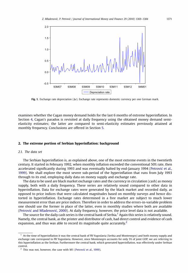
Fig. 1. Exchange rate depreciation (De). Exchange rate represents domestic currency per one German mark.

Z. Mladenovi�c, P. Petrovi�c / Journal of International Money and Finance 29 (2010) 1369–1384 1371

examines whether the Cagan money demand holds for the last 6 months of extreme hyperinflation. InSection 4, Cagan’s paradox is revisited at daily frequency using the obtained money demand semi-elasticity estimates; the latter are compared to semi-elasticity estimates previously attained atmonthly frequency. Conclusions are offered in Section 5.

2. The extreme portion of Serbian hyperinflation: background

2.1. The data set

The Serbian hyperinflation is, as explained above, one of the most extreme events in the twentiethcentury. It started in February 1992, when monthly inflation exceeded the conventional 50% rate, thenaccelerated significantly during 1993 and was eventually halted by end-January 1994 (Petrovi�c et al.,1999). We shall explore the most severe sub-period of the hyperinflation that runs from July 1993through to its end, employing daily data on money supply and exchange rate.

The data to be used are blackmarket exchange rates and the currency in circulation (cash) as moneysupply, both with a daily frequency. These series are relatively sound compared to other data inhyperinflation. Data for exchange rates were generated by the black market and recorded daily, asopposed to price indices that were calculated magnitudes based on monthly surveys and hence dis-torted in hyperinflation. Exchange rates determined in a free market are subject to much lowermeasurement error than are price indices. Therefore in order to address the errors-in-variable problemone should use the former in place of the latter, even in monthly studies where both are available(Petrovi�c and Mladenovi�c, 2000). At daily frequency, however, the price level data is not available.

The source for the daily cash series is the central bank of Serbia.1 Again this series is relatively sound.Namely, the central bank, as the printer and distributor of cash, had direct control and evidence of cashexpansion, and thus was able to record its magnitude quite accurately.2

1 At the time of hyperinflation it was the central bank of FR Yugoslavia (Serbia and Montenegro) and both money supply andexchange rate correspond to FR Yugoslavia. However, since Montenegro accounts for only 5% of joint GDP, we are referring tothis hyperinflation as the Serbian. Furthermore the central bank, which generated hyperinflation, was effectively under Serbiancontrol.

2 This was not, however, the case with M1 (Petrovi�c et al., 1999).

-0.4

0.0

0.4

0.8

1.2

1.6

2.0

2.4

93M07 93M08 93M09 93M10 93M11 93M12 94M01

Money growth Interpolated data

Fig. 2. Money growth (Dm).

Z. Mladenovi�c, P. Petrovi�c / Journal of International Money and Finance 29 (2010) 1369–13841372

An additional reason to opt for cash money is that the average share of cash in the base money wasaround 80%, representing the main source for seigniorage in the period considered. Finally, most ofclassical hyperinflations are also studied employing notes in circulations (Barro, 1970,1972).

The daily data for exchange rates is available for the whole period, i.e. through January 1994.However some observations on the cash money supply are missing in December and January, inparticular for December 13–19, and December 28–January 10 periods. We have interpolated them (seeFig. 2),3 and used this money series when analyzing the whole period as in Fig. 3. However, partly dueto missing data, the sample used for estimation runs through December. Also, it covers five workingdays per week, since the money supply did not change over weekends.

2.2. Money supply and exchange rate dynamics

The daily evolution of exchange rate depreciation (De) and money growth (Dm) are shown inFigs. 1 and 2, and in Table 1. The exchange rate depreciation (De) and the money growth (Dm)doubled in July as compared to June thus attaining a new plateau through October. Subsequently,they accelerated significantly again in November, December and January. The same pattern is fol-lowed by variability of these series as shown in Figs. 1 and 2, and by corresponding standarddeviations in Table 1. Econometric tests confirm the described pattern. Specifically, the daily seriesof Dm and De exhibited a structural break by the end of June increasing both in level and persis-tence, i.e. switching from stationary to non-stationary series.4 The latter even formally points to July1993 as the start of distinctive portion of hyperinflation, and motivates our choice of the period tobe examined. Additionally, variability of the series sharply increases in December and January (cf.

3 The exponential trend is used to interpolate logarithm of money supply (m). In addition, the level of money supply achievedon Friday is kept constant through Sunday, as there was no money creation over weekends.

4 Various tests are employed all suggesting a break in persistence by the end of June, first in money growth and then inexchange rate depreciation. The null hypothesis that the series (Dm and De) are I(1) throughout the sample against thealternative that the number of unit roots changes from 0 to 1 (Leybourne et al., 2003) is rejected in both cases. The test is basedon the Elliot-Rothenberg-Stock type of DF t-ratio (Elliott et al., 1996). A two-step procedure (Busetti and Taylor, 2004) esti-mating the break point in level and then testing change in persistence confirmed that both occurred by the end of June. Theresults are available from the authors upon request.

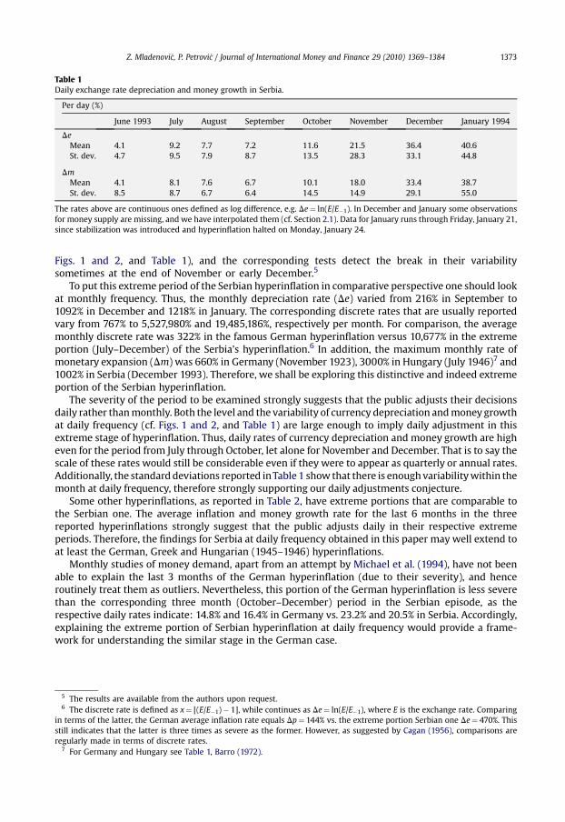
Table 1Daily exchange rate depreciation and money growth in Serbia.

Per day (%)

June 1993 July August September October November December January 1994

DeMean 4.1 9.2 7.7 7.2 11.6 21.5 36.4 40.6St. dev. 4.7 9.5 7.9 8.7 13.5 28.3 33.1 44.8

DmMean 4.1 8.1 7.6 6.7 10.1 18.0 33.4 38.7St. dev. 8.5 8.7 6.7 6.4 14.5 14.9 29.1 55.0

The rates above are continuous ones defined as log difference, e.g. De¼ ln(E/E�1). In December and January some observationsfor money supply are missing, and we have interpolated them (cf. Section 2.1). Data for January runs through Friday, January 21,since stabilization was introduced and hyperinflation halted on Monday, January 24.

Z. Mladenovi�c, P. Petrovi�c / Journal of International Money and Finance 29 (2010) 1369–1384 1373

Figs. 1 and 2, and Table 1), and the corresponding tests detect the break in their variabilitysometimes at the end of November or early December.5

To put this extreme period of the Serbian hyperinflation in comparative perspective one should lookat monthly frequency. Thus, the monthly depreciation rate (De) varied from 216% in September to1092% in December and 1218% in January. The corresponding discrete rates that are usually reportedvary from 767% to 5,527,980% and 19,485,186%, respectively per month. For comparison, the averagemonthly discrete rate was 322% in the famous German hyperinflation versus 10,677% in the extremeportion (July–December) of the Serbia’s hyperinflation.6 In addition, the maximum monthly rate ofmonetary expansion (Dm) was 660% in Germany (November 1923), 3000% in Hungary (July 1946)7 and1002% in Serbia (December 1993). Therefore, we shall be exploring this distinctive and indeed extremeportion of the Serbian hyperinflation.

The severity of the period to be examined strongly suggests that the public adjusts their decisionsdaily rather thanmonthly. Both the level and the variability of currency depreciation andmoneygrowthat daily frequency (cf. Figs. 1 and 2, and Table 1) are large enough to imply daily adjustment in thisextreme stage of hyperinflation. Thus, daily rates of currency depreciation and money growth are higheven for the period from July through October, let alone for November and December. That is to say thescale of these rates would still be considerable even if they were to appear as quarterly or annual rates.Additionally, the standarddeviations reported inTable 1 show that there is enoughvariabilitywithin themonth at daily frequency, therefore strongly supporting our daily adjustments conjecture.

Some other hyperinflations, as reported in Table 2, have extreme portions that are comparable tothe Serbian one. The average inflation and money growth rate for the last 6 months in the threereported hyperinflations strongly suggest that the public adjusts daily in their respective extremeperiods. Therefore, the findings for Serbia at daily frequency obtained in this paper may well extend toat least the German, Greek and Hungarian (1945–1946) hyperinflations.

Monthly studies of money demand, apart from an attempt by Michael et al. (1994), have not beenable to explain the last 3 months of the German hyperinflation (due to their severity), and henceroutinely treat them as outliers. Nevertheless, this portion of the German hyperinflation is less severethan the corresponding three month (October–December) period in the Serbian episode, as therespective daily rates indicate: 14.8% and 16.4% in Germany vs. 23.2% and 20.5% in Serbia. Accordingly,explaining the extreme portion of Serbian hyperinflation at daily frequency would provide a frame-work for understanding the similar stage in the German case.

5 The results are available from the authors upon request.6 The discrete rate is defined as x¼ [(E/E�1)� 1], while continues as De¼ ln(E/E�1), where E is the exchange rate. Comparing

in terms of the latter, the German average inflation rate equals Dp¼ 144% vs. the extreme portion Serbian one De¼ 470%. Thisstill indicates that the latter is three times as severe as the former. However, as suggested by Cagan (1956), comparisons areregularly made in terms of discrete rates.

7 For Germany and Hungary see Table 1, Barro (1972).

Table 2Inflation and money growth in extreme portion of hyperinflation. Average for the last 6 months, expressed per day (%).

Germany Greece Hungary II Serbia

Inflation (Dp) 9.9 (14.8) 8.3 4.9 15.6 (23.2)Money growth (Dm) 9.7 (16.4) 9.7 3.9 14.0 (20.5)

Averagemonthly inflation andmoney growth for the last 6months are expressed per day by dividingmonthly averages by 30. Inthe brackets are average rates for the last 3months. Source: Cagan (1956) for Germany and Greece, and Barro (1972) for HungaryII. For Serbia average money growth and currency depreciation as a measure of inflation are derived from Table 1.

Z. Mladenovi�c, P. Petrovi�c / Journal of International Money and Finance 29 (2010) 1369–13841374

2.3. Seigniorage and inflation tax

Seigniorage is calculated as daily changes in cashmoney over exchange rate, and inflation tax as realcash holdings multiplied by depreciation rate. These twomeasures are equal only in a steady state. Theresults are depicted in Table 3.

The data reported in Table 3 suggests the existence of the Laffer curve property. Namely seigniorageand inflation tax are both relatively stable from August onwards, reaching the maximum in Novemberand then declining in December and January. This development follows those of the exchange ratedepreciation (De) and money growth (Dm) through November (cf. Table 1). July is an outlier withseigniorage and inflation tax almost as high as in November, but withmoney growth and exchange ratedepreciation half of that in November. This result might be due to the sharp rise, i.e. doubling of moneygrowth and exchange rate depreciation in July which perhaps had not been anticipated. Namely, theseseries (De and Dm) exhibit a structural break both in level and persistence by the end of June. Hence theobservation for July could be off the Laffer curve.

With weekly observations, one finds that the maximum seigniorage is achieved in the last week ofNovember (22–28), while the maximum for inflation tax is attained a week later, i.e. the beginning ofDecember. Again, there is one outlier week in July.

Summarizing the trends explored above, we see that money growth and exchange rate depreciationrose abruptly in July 1993, remained relatively stable through October and then started to increaseagain. Accordingly, seigniorage and inflation tax were also initially stable, then increased and reachedthe maximum by the end of November 1993, and subsequently largely declined in December andJanuary. This suggests that the economy was on the efficient, increasing side of the Laffer curve all waythrough November, and on the wrong side in December and January. The latter has been reflected inthe movement of exchange rate depreciation (De) and money growth (Dm). Specifically, the daily dataindicates that, after surpassing themaximum of the Laffer curve by the end of November, exchange ratedepreciation (De) and money growth (Dm) surged and became considerably more volatile (cf. Table 1).

Thus the data suggests the existence of the inflation tax Laffer curve, and that the economy was onthe efficient side of the curve throughout the severe hyperinflation, with the exception of the last 2months (seven weeks). This evidence obtained at daily frequency for Serbia run against previousfindings in monthly studies, while suggesting that governments carry on with money printing as longas non-decreasing seigniorage could be extracted. The latter challenges Cagan’s paradox found atmonthly frequency, and supports the view that seigniorage collection can explain both what triggershyperinflation and how long it will last. However this evidence should and will be formally tested inwhat follows (cf. Section 3).

Table 3Seigniorage and inflation tax in Serbia. Average per day, million German marks.

June 1993 July August September October November December 1–12and 20–27

January 11–21

Seigniorage 2.4 3.4 3.1 2.6 2.9 3.5 2.9 1.5Inflation tax 2.3 3.9 3.2 2.8 3.3 3.9 3.0 1.4

In December and January some observations for money supply are missing, hence we report sub-periods for which data isavailable.

Z. Mladenovi�c, P. Petrovi�c / Journal of International Money and Finance 29 (2010) 1369–1384 1375

2.4. Evolution of real money balances

Real money balances, defined as currency in circulation over exchange rate, or in logs, (m� e),exhibit movement consistent with the Cagan money demand schedule.

As shown in Fig. 3, real money balances are relatively stable in the period from July throughSeptember 1993, when money growth (Dm) and exchange rate depreciation (De) are also stable (cf.Table 1). The sharp decrease in real money holdings during November and December coincides withthe surge in hyperinflation. Thus developments of real money balances from July through Decemberseem consistent with the Cagan money demand schedule. However, demonetization was halted inJanuary 1994 despite extreme rates of money growth and currency depreciation. The latter may be dueto the announcement of stabilization, first for the beginning of January and then postponed until theJanuary 24when it was enacted. Additionally half of themoney data points for January are missing (seeFig. 2), and the interpolated observations used instead might be prone to measurement error. All thismotivates us to skip January from the sample used to estimate money demand.

3. Estimating Cagan money demand

The Cagan money demand model we shall be looking at is:

mt � et ¼ �aEtðetþ1 � etÞ þ ut (1)

The mt and et are the natural logarithms of money and exchange rate, respectively, Et is theconditional expectation operator, coefficient a is the semi-elasticity of money demand, and ut isstationary velocity shock.

Themodel differs from the standard one in replacing the price level with the exchange rate. It can bethought of as the reduced form obtained by substituting out prices in the standard model using thepurchasing power parity hypothesis.

Alternatively, one may argue that in hyperinflation the exchange rate behavior better reflects trueinflation dynamics than do actual price movements. Beside an error-in-variables argument advancedabove, one should invoke almost complete dollarization of an economy in hyperinflation. This meansthat practically all prices are set and most transactions performed in foreign currency, but also that thepublic expresses relevant magnitudes like real money, income, etc. in foreign money as well. Conse-quently economic agents look at the exchange rate movements rather than at those of prices whilemaking their decisions in hyperinflation. This then suggests that exchange rate developments both

0.0

0.5

1.0

1.5

2.0

2.5

3.0

3.5

4.0

93M07 93M08 93M09 93M10 93M11 93M12 94M01

Real money

Fig. 3. Real money (m� e).

Table 4Unit root testing (period: July 1–December 31, 1993).

et mt mt� et

Augmented Dickey-FullerHo: I(3)H1: I(2)

�18.55 �15.89

Ho: I(2)H1: I(1)

�1.23 �1.03 �8.35

Ho: I(1)H1: I(0)

�3.02

Kwiatkowski–Phillips–Schmidt–ShinHo: I(2)H1: I(3)

0.005 0.009

Ho: I(1)H1: I(2)

0.29 0.29 0.018

Ho: I(0)H1: I(1)

1.78

The number of lags in ADF and KPSS tests is chosen as a minimum number of lags that eliminates autocorrelation. The number ofcorrections is equal to 9 for exchange rate and money, and 0 for real money. The unit root tests are based on the model withconstant and trend with the 5% critical value for ADF test –3.45 (MacKinnon, 1991). The corresponding 5% critical value for theKPSS test is 0.15 (Kwiatkowski et al., 1992). The 5% critical value for the right tail of the ADF distribution is –0.90 in the modelwith constant and trend (Fuller, 1976).

Z. Mladenovi�c, P. Petrovi�c / Journal of International Money and Finance 29 (2010) 1369–13841376

influence and reflect the public’s behavior, and hence should be a better proxy for expected inflationthan the actual inflation rate. Moreover, one may also argue that the exchange rate is determineddirectly in the money market and not through relative price levels, and the Cagan model abovecaptures this feature. In fact there is already some empirical evidence on the German (Engsted, 1996)and the Serbian (Petrovi�c and Mladenovi�c, 2000) hyperinflations that support the latter hypothesis.Additionally, some support is found even in a panel of 19 low-inflation developed economies (Markand Sul, 2001).8

In monthly studies of high and hyperinflation (e.g. Taylor, 1991; Phylaktis and Taylor, 1993; Engsted,1994; Petrovi�c and Vujo�sevi�c, 1996) it has beenwell documented that real money balances cointegratewith inflation rate, hence supporting the Cagan money demand. Moreover, the existence of thiscointegration implies a super-consistent estimate of money demand semi-elasticity that holds fora wide array of expectations formation schemes. We shall now explore whether the same patternemerges at daily frequencies in the severe portion of hyperinflation. Interestingly enough, the coin-tegration between real money balances and inflation rate was not found in a rare hyperinflation studyat weekly frequency done for the 1945–1946 Hungarian episode (Engsted, 1998).

Accordingly, we shall test first if money (m) and exchange rate (e) are I(2) processes, and whetherthey cointegrate such that real money balances (m� e) are I(1) process. If so, one can proceed toestimate the Cagan money demand above by testing for cointegration between real balances (m� e)and exchange rate depreciation (De), and obtaining the cointegrating vector. Alternatively, a semi-elasticity of money demand (a) estimate can be obtained from the cointegrating vector between realbalances (m� e) and money growth (Dm). The latter cointegration precludes the presence of bubblesand indicates forward looking behavior (Engsted, 1994).

As explained in Section 2 the sample runs from July 1 to December 31, 1993 and covers fiveworkingdays per week. Table 4 summarizes the results on unit root testing.

Reported results do indeed confirm that both money (m) and exchange rate (e) are I(2) processes,and hence respective first differences Dm and De are I(1) processes. Thus the obtained ADF statisticsshow that the null hypothesis stating thatm and e are I(2) cannot be rejected, while the one stating thatthey are I(3) can. The KPSS test also gives the same results. Namely, the null thatm and e are I(2) against

8 Mark and Sul conclude that an explanation for their results “. may be that the long-run nominal exchange rate isdetermined directly by monetary fundamentals and not by relative price levels” (Mark and Sul, 2001, p. 47).

Table 5Testing for the break in currency depreciation (De) and money growth (Dm): the Zivot–Andrews unit root test (Period: July1–December 31, 1993).

Break in the meanof trend function

Break in the slopeof trend function

Break in the mean andslope of trend function

MinimumADF

Date of minimumvalue

MinimumADF

Date of minimumvalue

MinimumADF

Date of minimumvalue

Det �2.79 December, 6, 1993 �3.12 October 20, 1993 �3.11 November 1, 1993Dmt �3.01 December, 6, 1993 �3.79 November 1, 1993 �3.79 December 6, 1993

The 5% critical values for the Zivot–Andrews ADF tests are�4.80,�4.42 and�5.08, respectively, for themodel that allows for thebreak in the mean, in the slope and in the both. There are nine lags in the model for Det and eight in the model for Dmt.

Z. Mladenovi�c, P. Petrovi�c / Journal of International Money and Finance 29 (2010) 1369–1384 1377

the alternative of being I(3) is not rejected, while the null thatm and e are I(1) is rejected in favor of thealternative that they are I(2). Additionally, both ADF and KPSS tests show that money (m) and exchangerate (e) cointegrate making real money balances (m� e) an I(1) process (cf. Table 4).

Furthermore, these processes are not explosive. Namely, the right tail critical value of the ADF testcan be used to test whether the processes (m� e), Dm and De are I(1) or explosive. Since all calculatedvalues of the ADF test are less than the corresponding 5% right tail critical value, we may conclude thatthe time series considered do not contain an explosive root. Specifically, the ADF test for Dm and De,being�1.03 and�1.23 respectively are lower thanmatching 5% right tail (�0.90); in case of real moneybalances ADF test (�3.02) is also lower than this critical value.

As shown in Section 2 (cf. Figs. 1 and 2, and Table 1) currency depreciation (De) and money growth(Dm) sharply increased by the end of November, suggesting that these series might have experienceda break in their respective means. In order to examine this, the Zivot and Andrews (1992) unit root testis used while testing whether depreciation (De) and money growth (Dm) are respectively unit rootprocesses or stationary variables with a single break. Thus we tested for the break in the mean(intercept) of these series, but also for the break in their slopes and then in both, at the unknown pointin time. The sample covers thewhole period, i.e. July 1–December 31,1993, and the results are reportedin Table 5.

Because in each case explored in Table 5 the minimum value of the ADF test is greater than thecorresponding 5% critical value, one cannot reject the null hypothesis that (De) and (Dm) are unit rootprocesses, implying further that they do not exhibit a break.

The results reported in Tables 4 and 5 clear the way for estimating the Cagan money demand.Namely, one can proceed and explore cointegration of real money balances (m� e) with exchange ratedepreciation (De) and money growth (Dm) respectively. The results are presented in Table 6.9

In both cases, tests employed do confirm the presence of cointegration. Neither process is explosive,i.e. there is no root larger than one, which confirms the results reported above. Alternative semi-elasticity estimates are very close to each other: 5.00 and 5.37. Thus the estimated Cagan moneydemand seems to be stable even through December 31, hence encompassing the period of the greatsurge in money growth and exchange rate depreciation as well as the rise in their volatility.

Nevertheless we formally examined the stability of the Caganmoney demand using diagnostic testsbased on recursive estimation of a cointegrated VARmodel. The model explored is the onewith moneygrowth (Dm)10 and results are depicted in Figs. 4 and 5. Fig. 4 shows the test statistics for the max testfor constancy of cointegration parameters advocated by Hansen and Johansen (1999),11 with simulatedcritical values reported in Dennis (2006).

Values of the test statistics are divided by the 5% critical value, and hence the obtained magnitudesthat are less than one suggest parameter stability. As all of them are below one (see Fig. 4) we cannotreject the null hypothesis that the cointegration parameters are constant for the whole sample.Specifically, although the test statistics spike by the end of November, as could be expected (cf. Figs. 1

9 The VAR model that is used for cointegration testing is reported in the Appendix.10 The same results are obtained for the version with currency depreciation (De).11 It is the LM type test for parameter constancy originally suggested by Nyblom (1989).

Table 6Cointegration test and estimation of cointegrating vectors (period: July 1–December 31, 1993).

Cointegration between (m� e) and De

Rank Eigenvalue Trace test Cointegrating vector

mt� et Det 1

r¼ 0 0.145 22.17 1 5.00 �4.13r� 1 0.028 3.37 (0.38) (0.07)The largest roots of the companion matrix (r¼ 1): 1.00, 0.94, 0.94, 0.94, 0.93, 0.93, 0.91, 0.91, 0.89, 0.89.

Cointegration between (m� e) and Dm

Rank Eigenvalue Trace test Cointegrating vector

mt� et Dmt 1

r¼ 0 0.168 24.09 1 5.37 �4.13r� 1 0.010 1.28 (0.42) (0.09)The largest roots of the companion matrix (r¼ 1): 1.00, 0.89, 0.89, 0.85, 0.85, 0.78, 0.78, 0.77, 0.76, 0.76

A constant term is restricted to entering a cointegration vector only. There are eight lags in the VARmodel of (m� e) andDm, andtwelve lags in the VARmodel of (m� e) and De. Dummy variables are included in the VAR to model outliers that are identified asextreme values of standardized VAR residuals. The VAR model of (m� e) and Dm contains the following dummy variables: D1,D2, D3, D4, D5, D6, D7, D8 and D9. These dummy variables are defined as follows: D1¼ 1 for 1993:07:26 and 0 otherwise,D2¼�1 for 1993:10:1, 1993:10:4 and 0 otherwise, D3¼ 1 for 1993:10:11 and 0 otherwise, D4¼ 1 for 1993:11:1 and 0 other-wise, D5¼ 1 for 1993:09:13 and 0 otherwise, D6¼ 1 for 1993:11:29 and 0 otherwise, D7¼ 1 for 1993:12:6 and 0 otherwise,D8¼ 1 for 1993:12:16 and 0 otherwise and D9¼ 1 for 1993:12:24,�1 for 1993:12:27 and 0 otherwise. The VARmodel of (m� e)and De contains the following dummy variables: D1, D2, D4, D6, D8 and D10. Dummy variable D10 is defined as follows: D10¼ 1for 1993:11:17, 1993:11:18 and 0 otherwise. The 5% critical values for the trace test are simulated with 10000 replications usingCATS in RATS 2.0 (Dennis, 2006). In the VARmodel of (m� e) and Dm, the 5% critical values are: 19.93 for r¼ 0 and 9.19 for r� 1.In the VAR model of (m� e) and De, the 5% critical values are: 20.33 for r¼ 0 and 9.31 for r� 1. Standard errors of estimatedcointegration parameters are given in parentheses.

0.0

0.1

0.2

0.3

0.4

0.5

0.6

0.7

0.8

0.9

1.0

11/15/93 11/22/93 11/29/93 12/6/93 12/13/93 12/20/93 12/27/93

X(t)R(t)5% Critical value (2.18=Index)

Fig. 4. Recursively computed max test of constant cointegration parameters. X stands for the model with the original variables whileR denotes results based on variables corrected for short-term dynamics and interventions (cf. Juselius, 2006).

Z. Mladenovi�c, P. Petrovi�c / Journal of International Money and Finance 29 (2010) 1369–13841378

3.0

3.5

4.0

4.5

5.0

5.5

6.0

6.5

7.0

7.5

11/15/93 11/22/93 11/29/93 12/6/93 12/13/93 12/20/93 12/27/93

+95% confidence bandEstimated money demand semi-elasticity-95% confidence band

Fig. 5. Recursively computed semi-elasticity estimates. Version of the Cagan model with money growth (Dm) is used. Model withoriginal variables is employed (cf. note to Fig. 4).

Z. Mladenovi�c, P. Petrovi�c / Journal of International Money and Finance 29 (2010) 1369–1384 1379

and 2, and Table 1), they are still well below the critical value hence indicating the constancy of theCagan money demand parameters.

In accordancewith the results above, the semi-elasticity of money demand also turns out to be quitestable over the turbulent months of November and December. This is demonstrated by its recursivelycomputed estimates depicted in Fig. 5.

In summary, the Cagan money demand is accepted at daily frequency for the most severe period ofthe Serbian hyperinflation since real money balances (m� e) cointegrate with currency depreciation(De) and money growth (Dm) respectively, and the estimated relations prove to be stable. Theacceptance of this money demand is independent of expectations formation, and may encompass bothadaptive and rational expectations.

4. Cagan’s paradox revisited

We shall now look at how the Cagan model, specifically the estimated money demand semi-elas-ticity, concurs with the observed pattern of inflation tax, i.e. its bell shape with non-decreasinginflation tax through November 1993 and subsequent drop in December and January (cf. Table 3).

Following Drazen (1985), the standard measures of the revenues arising from inflation in our casewould be, respectively, monetary growth Dm and depreciation rate De multiplied by real moneyholdings (m� e).

As to the former (Dm), the corresponding estimate of money demand semi-elasticity is 5.37 (cf.Table 6), implying that the money growth rate of 18.6% per day maximizes revenue from inflation.The actual rate of monetary expansion (cf. Table 1) was below the maximizing one throughOctober, reached it in November (18%), and surpassed the maximizing rate in December andJanuary. The latter suggests that through November the economy was on the increasing side of theLaffer curve and subsequently, in December and January, on the decreasing side. The same result is

Z. Mladenovi�c, P. Petrovi�c / Journal of International Money and Finance 29 (2010) 1369–13841380

obtained for the alternative measure that employs exchange rate depreciation (De). Specifically,the corresponding semi-elasticity estimate is 5.00 (cf. Table 6), leading to a Laffer’s curve maxi-mizing rate of 20% per month. The comparison with the actual average currency depreciation rates(cf. Table 1) in November (21.5%) and December (36.4%) shows again that the economy reachedthe maximum of the Laffer curve in November, and then switched to the wrong, decreasing side ofthe curve.

Looking more closely i.e. at the weekly data, one finds that monetary expansion exceeded themaximizing rate (18.6%) in the week of November 15–21 (23% per day), then dropped below it in thesubsequent week (10.5%), and finally surpassed it in the week of November 29–December 5 (35.5%).The same pattern, only lagging by one week, is observed for the alternative measure, i.e. inflation tax.Thus the actual rate (27.1%) conclusively exceeded the maximizing rate (20%) in the week of December6–12.

Accordingly the estimated Cagan model suggests that the maximum of the Laffer curve is attainedsometime at the end of November or in early December 1993. So the economy was on the increasingside of the Laffer curve through the end of November and on the wrong side only for the subsequent,last 2 months (seven weeks) of hyperinflation. This pattern concurs with the actual evolution ofseigniorage and inflation tax as shown in Section 2. It follows that daily data estimates clearly reject theCagan’s paradox.

The daily results above diverge from those obtained at monthly frequency for the Serbian episode.Thus even the monthly estimates that allow for decreasing semi-elasticity of money demand, althoughpointing in the right direction nevertheless fall short of resolving Cagan’s paradox. Namely, the esti-mated Barro’s (1970, 1972) model for the Serbian episode at monthly frequency suggests thatthe economy was on the wrong side of the Laffer curve for the last 6 months of hyperinflation,12 whilethe corresponding estimate of Easterly et al. (1995) schedule positions the Serbian economy on thedecreasing side of Laffer curve for as long as 14 months.13 These results contradict both the actualinflation tax evolution depicted in Table 3, and daily data estimates. Thus at monthly frequency evendecreasing semi-elasticity of money demand cannot capture the true hyperinflation dynamics,specifically throughout its last extreme portion.

Confronting our daily data results with comparable Cagan money demand estimates at monthlyfrequency for other hyperinflations points to stark differences (see Table 7).

As shown in Table 7 monthly semi-elasticity estimates vary from 3 to 6, even 8, while our dailyestimates (5.00–5.37) expressed at monthly frequency are as small as 0.17–0.18. Moreover, the reportedmonthly studies of hyperinflation do support Cagan’s paradox, positioning economies on thedecreasing segment of the Laffer curve for the significant period of hyperinflation. Namely, as shown inTable 7, the average inflation rate is higher than the one that maximizes the Laffer curve in all but onecase, and statistical tests confirm this (Taylor, 1991). These studies hence imply that in hyperinflationgovernments continue expanding the money supply at an increasing rate even when the resultingseigniorage is declining, thus creating Cagan’s paradox. Namely, the puzzle is why governments opt forhigher rates of money growth and inflation when they can collect the same amount of seigniorage atthe lower rates.

Contrary to these monthly studies, analysis at daily frequency plainly rejects Cagan’s paradox, i.e.the results indicate that the government succeeded in collecting non-decreasing seigniorage almostthrough the end of hyperinflation. This explains why the Serbian government carried on with moneycreation at an accelerating rate throughout the episode. Thus daily data findings clearly demonstratethat hyperinflation is triggered and driven by government’s need for seigniorage. As opposed tomonthly studies, daily results can also explain why hyperinflation lasts as long as it does, by showingthat governments continue expanding the money supply at an increasing rate up to the point whenseigniorage starts collapsing. In broad picture, the results at daily frequency strongly support thefiscal view of hyperinflation, stating that governments revert to money printing to cover

12 The results are available from the authors upon request.13 Cf. Petrovi�c and Mladenovi�c (2000).

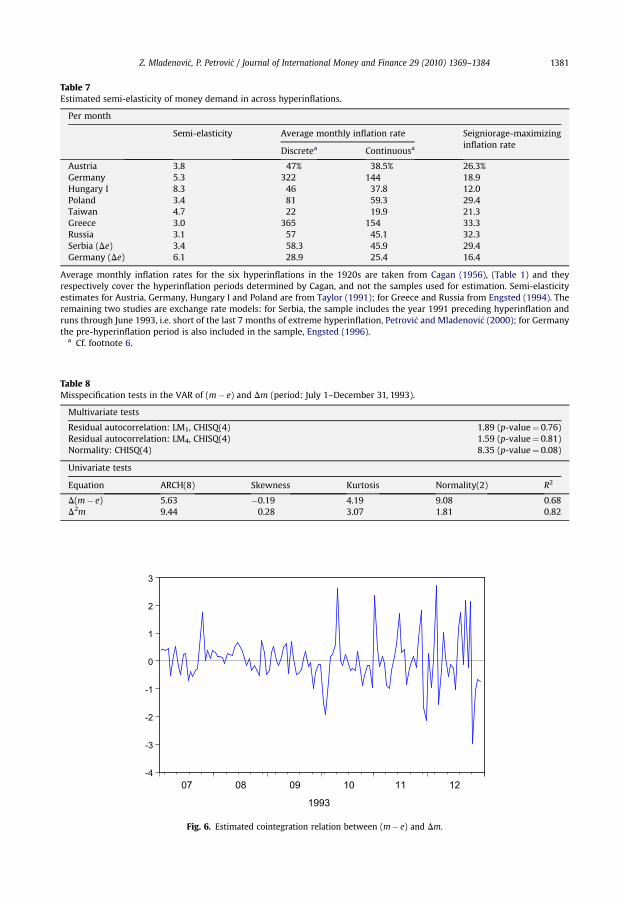
Table 7Estimated semi-elasticity of money demand in across hyperinflations.

Per month

Semi-elasticity Average monthly inflation rate Seigniorage-maximizinginflation rate

Discretea Continuousa

Austria 3.8 47% 38.5% 26.3%Germany 5.3 322 144 18.9Hungary I 8.3 46 37.8 12.0Poland 3.4 81 59.3 29.4Taiwan 4.7 22 19.9 21.3Greece 3.0 365 154 33.3Russia 3.1 57 45.1 32.3Serbia (De) 3.4 58.3 45.9 29.4Germany (De) 6.1 28.9 25.4 16.4

Average monthly inflation rates for the six hyperinflations in the 1920s are taken from Cagan (1956), (Table 1) and theyrespectively cover the hyperinflation periods determined by Cagan, and not the samples used for estimation. Semi-elasticityestimates for Austria, Germany, Hungary I and Poland are from Taylor (1991); for Greece and Russia from Engsted (1994). Theremaining two studies are exchange rate models: for Serbia, the sample includes the year 1991 preceding hyperinflation andruns through June 1993, i.e. short of the last 7 months of extreme hyperinflation, Petrovi�c and Mladenovi�c (2000); for Germanythe pre-hyperinflation period is also included in the sample, Engsted (1996).

a Cf. footnote 6.

Table 8Misspecification tests in the VAR of (m� e) and Dm (period: July 1–December 31, 1993).

Multivariate tests

Residual autocorrelation: LM1, CHISQ(4) 1.89 (p-value¼ 0.76)Residual autocorrelation: LM4, CHISQ(4) 1.59 (p-value¼ 0.81)Normality: CHISQ(4) 8.35 (p-value¼ 0.08)

Univariate tests

Equation ARCH(8) Skewness Kurtosis Normality(2) R2

D(m� e) 5.63 �0.19 4.19 9.08 0.68D2m 9.44 0.28 3.07 1.81 0.82

-4

-3

-2

-1

0

1

2

3

07 08 09 10 11 12

1993

Fig. 6. Estimated cointegration relation between (m� e) and Dm.

Z. Mladenovi�c, P. Petrovi�c / Journal of International Money and Finance 29 (2010) 1369–1384 1381

-.8

-.6

-.4

-.2

.0

.2

.4

.6

07 08 09 10 11 12

1993

Fig. 7. Estimated cointegration relation between (m� e) and Dm corrected for short-run effects and outliers.

Z. Mladenovi�c, P. Petrovi�c / Journal of International Money and Finance 29 (2010) 1369–13841382

unsustainable fiscal deficits, and that this lasts as long as they succeed in extracting sufficientinflation revenues.

5. Conclusions

The paper offers twomain results. First it shows that the Cagan (1956) money demand holds at dailyfrequency in the extreme portion of Serbia’s 1992–1993 hyperinflation, i.e. during its last 6 months.This result strongly supports a conjecture that in advanced hyperinflation the public adjusts theirdecisions daily, hence calling into question the findings of previous hyperinflation studies done asa rule at monthly frequency. Second, the obtained semi-elasticity estimates reject Cagan’s (1956)paradox, by showing that the economy has been on the correct, increasing side of the Laffer curvealmost through the end of hyperinflation. The latter result is in sharp contrast with those previouslyfound in monthly studies.

Namely, we obtained semi-elasticity estimates of money demand at daily frequency that are farlower than the those derived from monthly studies. Thus a representative daily semi-elasticityestimate (5.37) expressed at monthly frequency is just 0.18 (0.015 annually), which is about twentytimes lower than previous monthly estimates for hyperinflation (cf. Table 7). The inverse of semi-elasticity gives the inflation tax maximizing rate, and it is found to be 559% per month. This is farabove the comparable monthly estimates, which imply a maximizing rate in the range of 17–33% permonth.

The low value of money demand semi-elasticity is crucial in addressing Cagan’s paradox. Thus inthe Serbian episode, estimated semi-elasticity implies that money printing and the consequentcurrency depreciation did not result in the decrease of the inflation tax through the severe period ofhyperinflation, except for the last 2 months (seven weeks). The actual inflation tax path concurs withthe pattern predicted by the model, both in terms of the bell shape of the Laffer curve and in thetiming of the maximum. These results point out that the government’s demand for seigniorage forcedthe Serbian economy into hyperinflation and that it lasted almost as long as non-decreasingseigniorage could be extracted. This resolves Cagan’s paradox in the case of the Serbianhyperinflation.

On the other hand, monthly estimates in Serbia (even those allowing for decreasing semi-elasticity)could not capture actual inflation tax evolution, and significantly differ from daily results. Theseestimates do point in the right direction, i.e. that semi-elasticity decreases as inflation accelerates,however not enough to resolve Cagan’s paradox. Thus even varying semi-elasticity money demandschedules (e.g. Barro, 1970; Easterly et al., 1995) at monthly frequency fall short of explaining hyper-inflation dynamics and particularly that of inflation tax in the Serbian episode.

Z. Mladenovi�c, P. Petrovi�c / Journal of International Money and Finance 29 (2010) 1369–1384 1383

The semi-elasticity estimates at daily frequency are robust, i.e. they are obtained from cointegrationvectors using a large sample of around 130 daily observations that cover the most extreme portion ofhyperinflation. This markedly differs from the previous monthly hyperinflation studies that used only20–35 observations including relatively low rates of inflation. Both, the small sample and the inclusionof these low ratesmay have led to inferior monthly estimates and specifically to underestimation of theinflation tax maximizing rate (Barro, 1972).

However, the main reason for the discrepancy between daily and monthly estimates is mostprobably due to temporal aggregation of essentially daily processes into monthly ones, which whenused for modeling may indeed mask true relationships (cf. Taylor, 2001). Namely, we have found thatthe public adjusts daily in hyperinflation, and consequently monthly sampling might not reveal trueprocesses, implying further that monthly estimates could be unreliable.

The results obtained at daily frequency for the Serbian episode, specifically low semi-elasticity ofmoney demand and the consequent rejection of Cagan’s (1956) paradox, may well hold in otherhyperinflations. Thus, as in the Serbian case, some monthly studies for other episodes hint that semi-elasticity decreases as inflation accelerates, however not enough to resolve Cagan’s paradox (Barro,1970, 1972; Michael et al., 1994). But even more importantly, the severe portions of a few otherepisodes, notably those of Germany, Hungary (1945–1946) and Greece, are similar to that of Serbiahence suggesting that the public, in these cases also adjusts at daily frequency. The latter throws doubton the corresponding monthly estimates and hence on the presence of Cagan’s paradox that followsfrom them.

Acknowledgements

We thank the editor James Lothian and two anonymous referees for helpful comments andsuggestions. We also thank Jeffrey Frankel for constructive comments on a very early version of thispaper. Remaining errors, if any, rest with authors.

Appendix

The VAR models that are used for cointegration testing perform well statistically. This isdocumented below where some misspecification multivariate and univariate tests of the VAR for(m� e) and Dm are presented. Thus the multivariate tests for residual normality and first andfourth order residual correlation do not suggest misspecification (Table 8). We also reportedfollowing univariate tests and statistics based on the estimated residuals from each equation: testfor ARCH of order eight, Doornik–Hansen test of normality, estimated coefficients of skewness andkurtosis and R2. These tests are valid irrespective of whether the variables are I(0), I(1) or explo-sive, and hence can be performed as a first step independently of subsequent unit root testing(Nielsen, 2006; Engler and Nielsen, 2009). Estimated cointegration relation is depicted in Figs. 6and 7.

References

Barro, R.J., 1970. Inflation, payments period, and the demand for money. Journal of Political Economy 78, 1228–1263.Barro, R.J., 1972. Inflationary finance and the welfare cost of inflation. Journal of Political Economy 80, 978–1001.Busetti, F., Taylor, A.M.R., 2004. Tests of Stationarity against a change in persistence. Journal of Econometrics 123, 33–66.Cagan, P., 1956. The monetary dynamics of hyperinflation. In: Friedman, M. (Ed.), Studies in the Quantity Theory of Money.

Chicago University Press.Dennis, J.G., 2006. CATS in RATS. Estima, Evanston, IL.Drazen, A., 1985. A general measure of inflation tax revenues. Economic Letters 17, 327–330.Easterly, W., Mauro, P., Schmidt-Hebell, K., 1995. Money demand and seigniorage-maximizing inflation. Journal of Money,

Credit, and Banking 25, 584–603.Elliott, G., Stock, J.H., Rothenberg, T., 1996. Efficient tests for an autoregressive unit root. Econometrica 64, 813–836.Engler, E., Nielsen, B., 2009. The empirical process of autoregressive residuals. Econometrics Journal 12, 367–381.Engsted, T., 1994. The classic European hyperinflations revisited: testing the Cagan model using a cointegrated VAR approach.

Economica 61, 331–343.Engsted, T., 1996. The monetary model of the exchange rate under hyperinflation. Economics Letters 51, 37–44.

Z. Mladenovi�c, P. Petrovi�c / Journal of International Money and Finance 29 (2010) 1369–13841384

Engsted, T., 1998. Money demand during hyperinflation: cointegration, rational expectations, and the importance of moneydemand shocks. Journal of Macroeconomics 20, 533–552.

Friedman, M., 1971. Government revenue from inflation. Journal of Political Economy 79, 846–856.Fuller, W.A., 1976. Introduction to Statistical Time Series. Wiley, New York.Hansen, H., Johansen, S., 1999. Some tests for parameter constancy in cointegrated VAR model. Econometrics Journal 2,

306–333.Juselius, K., 2006. The Cointegrated VAR Model: Methodology and Applications. Oxford University Press, Oxford.Kwiatkowski, D., Phillips, P.C.B., Schmidt, P., Shin, Y., 1992. Testing the null hypothesis of stationarity against the alternative of

a unit root: how sure are we that economic time series have a unit root? Journal of Econometrics 54, 159–178.Leybourne, S., Kim, T.H., Smith, V., Newbold, P., 2003. Tests for a change in persistence against the null of difference-stationarity.

Econometrics Journal 6, 290–310.MacKinnon, J.G., 1991. Critical values for cointegration tests. In: Engle, R.F., Granger, C.W.J. (Eds.), Long-Run Economic Rela-

tionships: Readings in Cointegration. Oxford University Press, Oxford, pp. 267–276.Mark, N.C., Sul, D., 2001. Nominal exchange rates and monetary fundamentals: evidence from a small Post-Bretton Woods

panel. Journal of International Economics 53, 29–52.Michael, P., Nobay, A.R., Peel, D.A., 1994. The German hyperinflation and the demand for money revisited. International

Economic Review 35, 1–22.Nielsen, B., 2006. Order determination in general vector autoregressions. In: Ho, H.C., Ing, C.K., Lai, T.L. (Eds.), Time Series and

Related Topics: In Memory of Ching-Zong Wei. IMS Lecture Notes and Monograph Series 58, pp. 93–112.Nyblom, J., 1989. Testing for the constancy of parameters over time. Journal of the American Statistical Association 84, 223–230.Phylaktis, K., Taylor, M.P., 1993. Money demand, the Cagan model, and inflation tax: some Latin American evidence. Review of

Economics and Statistics 75, 32–37.Petrovi�c, P., Vujo�sevi�c, Z., 1996. The monetary dynamics in the Yugoslav hyperinflation of 1992–1993: the Cagan money

demand. The European Journal of Political Economy 12, 467–483. Erratum, 1997. The European Journal of Political Economy13, 385.

Petrovi�c, P., Bogeti�c, Z., Vujo�sevi�c, Z., 1999. The Yugoslav hyperinflation of 1992–1994: causes, dynamics and money supplyprocess. Journal of Comparative Economics 27, 335–353.

Petrovi�c, P., Mladenovi�c, Z., 2000. Money demand and exchange rate determination under hyperinflation: conceptual issues andevidence from Yugoslavia. Journal of Money, Credit and Banking 32, 785–806.

Taylor, A.M., 2001. Potential pitfalls for the purchasing-power-parity puzzle? Sampling and specification biases in mean-reversion tests of the law of one price. Econometrica 69, 473–498.

Taylor, M.P., 1991. The hyperinflation model of money demand revisited. Journal of Money, Credit and Banking 23, 327–351.Zivot, E., Andrews, D.W.K., 1992. Further evidence on the great crash, the oil price shock and the unit root hypothesis. Journal of

Business and Economic Statistics 10, 251–270.