CONTENTS - Lenders Compliance Group
15
Annales Academiæ Scientiarum Fennicæ Mathematica Volumen 37, 2012, 175–189 RENORMALIZED SOLUTIONS FOR A NON-UNIFORMLY PARABOLIC EQUATION Chao Zhang * and Shulin Zhou Harbin Institute of Technology, Department of Mathematics Harbin 150001, P. R. China; [email protected] Peking University, LMAM, School of Mathematical Sciences Beijing 100871, P. R. China; [email protected] Abstract. In this paper we prove the existence of nonnegative renormalized solutions for the initial-boundary value problem of a non-uniformly parabolic equation. Some well-known parabolic equations are the special cases of this equation. 1. Introduction Suppose that Ω is a bounded domain of R N (N ≥ 2) with Lipschitz boundary ∂ Ω, and T is a positive number. Denote Ω T =Ω × (0,T ], Σ= ∂ Ω × (0,T ]. In this paper we study the following non-uniformly parabolic initial-boundary value problem (1.1) u t - div ( D ξ Φ(∇u) ) = f in Ω T , u(x, t)=0 on Σ, u(x, 0) = u 0 (x) on Ω, where Φ: R N 7→ R + is a C 1 nonnegative, strictly convex function, D ξ Φ: R N → R represents the gradient of Φ(ξ ) with respect to ξ and ∇u represents the gradient with respect to the spatial variables x. Without loss of generality we may assume that Φ(0) = 0. Our main assumptions are that Φ(ξ ) satisfies the super-linear condition (or 1- coercive condition, see [23, Chapter E]) (1.2) lim |ξ|→∞ Φ(ξ ) |ξ | = ∞, and the symmetric condition: there exists a positive number C> 0 such that (1.3) Φ(-ξ ) ≤ C Φ(ξ ), ξ ∈ R N . In this paper we assume (1.4) u 0 ∈ L 1 (Ω) and f ∈ L 1 (Ω T ) with (1.5) u 0 ≥ 0 and f ≥ 0. There are numerous examples of Φ(ξ ) satisfying structure assumptions (1.2) and (1.3). The well-known are listed as follows. doi:10.5186/aasfm.2012.3709 2010 Mathematics Subject Classification: Primary 35D05; Secondary 35D10. Key words: Renormalized solutions, existence, parabolic. * Corresponding author.
Transcript of CONTENTS - Lenders Compliance Group
Annales Academiæ Scientiarum FennicæMathematicaVolumen 37, 2012, 175–189
RENORMALIZED SOLUTIONS FORA NON-UNIFORMLY PARABOLIC EQUATION
Chao Zhang∗ and Shulin Zhou
Harbin Institute of Technology, Department of MathematicsHarbin 150001, P.R. China; [email protected]
Peking University, LMAM, School of Mathematical SciencesBeijing 100871, P.R. China; [email protected]
Abstract. In this paper we prove the existence of nonnegative renormalized solutions for theinitial-boundary value problem of a non-uniformly parabolic equation. Some well-known parabolicequations are the special cases of this equation.
1. Introduction
Suppose that Ω is a bounded domain of RN (N ≥ 2) with Lipschitz boundary∂Ω, and T is a positive number. Denote ΩT = Ω × (0, T ], Σ = ∂Ω × (0, T ]. In thispaper we study the following non-uniformly parabolic initial-boundary value problem
(1.1)
ut − div(DξΦ(∇u)
)= f in ΩT ,
u(x, t) = 0 on Σ,
u(x, 0) = u0(x) on Ω,
where Φ: RN 7→ R+ is a C1 nonnegative, strictly convex function, DξΦ: RN → Rrepresents the gradient of Φ(ξ) with respect to ξ and ∇u represents the gradient withrespect to the spatial variables x. Without loss of generality we may assume thatΦ(0) = 0.
Our main assumptions are that Φ(ξ) satisfies the super-linear condition (or 1-coercive condition, see [23, Chapter E])
(1.2) lim|ξ|→∞
Φ(ξ)
|ξ| = ∞,
and the symmetric condition: there exists a positive number C > 0 such that
(1.3) Φ(−ξ) ≤ CΦ(ξ), ξ ∈ RN .
In this paper we assume
(1.4) u0 ∈ L1(Ω) and f ∈ L1(ΩT )
with
(1.5) u0 ≥ 0 and f ≥ 0.
There are numerous examples of Φ(ξ) satisfying structure assumptions (1.2) and(1.3). The well-known are listed as follows.
doi:10.5186/aasfm.2012.37092010 Mathematics Subject Classification: Primary 35D05; Secondary 35D10.Key words: Renormalized solutions, existence, parabolic.∗Corresponding author.
176 Chao Zhang and Shulin Zhou
Example 1.1.
Φ(ξ) =1
p|ξ|p, p > 1.
In this case, equation (1.1) is the parabolic counterpart of the p-Laplacian.
Example 1.2.
Φ(ξ) =1
p1
|ξ1|p1 +1
p2
|ξ2|p2 + · · ·+ 1
pN
|ξN |pN , pi > 1, i = 1, 2, . . . , N,
where ξ = (ξ1, ξ2, . . . , ξN). In this case, equation (1.1) is the parabolic counterpartof the anisotropic p-Laplacian. (See [25, Chapter 2].)
Example 1.3.Φ(ξ) = |ξ| log(1 + |ξ|).
(See [12, Chapter 4] and [20].)
Example 1.4.Φ(ξ) = |ξ|Lk(|ξ|),
where Li(s) = log(1+Li−1(s)) (i = 1, 2, . . . , k) and L0(s) = log(1+ s) for s ≥ 0. (See[22].)
Example 1.5.
Φ(ξ) = e|ξ|22 − 1.
(See [17], [24] and [28].)
Recently, Cai and Zhou [10] considered problem (1.1) without the right hand sidef under structure assumptions (1.2), (1.3) and integrability condition u0 ∈ L2(Ω) andproved the existence and uniqueness of weak solutions. This paper is a continuationof [10]. We are interested in the study of the well-posedness of problem (1.1) withL1 data. The existence techniques akin to the techniques of this paper were used inthe elliptic case by Boccardo and Gallouët in [7] and [8]. The first paper [7] also con-tained parabolic results, further developed in [6]. However, the counterexamples bySerrin, [32], indicated that with nontrivial right hand side uniqueness might fail whenn ≥ 3 with the usual definition. Thus some extra conditions on the distributionalsolutions were needed in order to ensure both existence and uniqueness. The threedifferent definitions for this purpose were independently introduced by Bénilan etal. [2] (entropy solutions), by Dall’Aglio [16] (SOLA, Solutions Obtained as Limit ofApproximations) and by Lions and Murat [27] (renormalized solutions, see also [20]).In the parabolic case, one should consult [16] (SOLA), [3] (renormalized solutions)and [29] (entropy solutions).
One result on this topic can be found in [34] where via the introduction of thenotion of entropy solutions. We proved that there exists an entropy solution forproblem (1.1) under assumptions (1.2), (1.3) and (1.4). Besides, in [33] we studiedthe following nonlinear parabolic problem
(1.6)
ut − div(|∇u|p(x)−2∇u
)= f in ΩT ,
u = 0 on Σ,
u(x, 0) = u0(x) on Ω,
Renormalized solutions for a non-uniformly parabolic equation 177
where the variable exponent p : Ω → (1, +∞) is a continuous function, f ∈ L1(ΩT )and u0 ∈ L1(Ω). We proved the existence and uniqueness of both renormalized so-lutions and entropy solutions for problem (1.6) and discovered the equivalence ofrenormalized solutions and entropy solutions. This motivates us to study problem(1.1) in the framework of renormalized solutions. The notion of renormalized so-lutions was first introduced by DiPerna and Lions [20] for the study of Boltamannequation. It was then adapted to the study of some nonlinear elliptic and parabolicproblems and evolution problems in fluid mechanics ([3, 4, 5, 9, 15, 26]). We hopethat the renormalized solution is still existent and unique, and it is equivalent tothe entropy solution of problem (1.1). However, so far we can only get the existenceof renormalized solutions for problem (1.1) under (1.2), (1.3), (1.4) and additional(1.5). The uniqueness of renormalized solutions and the equivalence of renormalizedsolutions and entropy solutions remain open. The main difficulty lies on that thereis no growth condition for function Φ(ξ). To our knowledge, growth conditions suchas polynomial growth or exponential growth for function Φ(ξ) played an extremelyimportant role, for example in [1, 11, 24], when parabolic problems or variationalproblems related to (1.1) were studied. If some condition such as ∆2-condition, i.e.,there exists a positive constant K such that for every ξ > 0 such that
Φ(2ξ) ≤ KΦ(ξ),
is further assumed on function Φ(ξ), it is possible to prove the uniqueness result ofthe renormalized solutions, and the equivalence of renormalized solutions and entropysolutions for problem (1.1) without the nonnegativity assumption (1.5).
Let Tk denote the truncation function at height k ≥ 0:
Tk(r) = mink, maxr,−k =
k if r ≥ k,
r if |r| < k,
−k if r ≤ −k,
and its primitive Θk : R → R+ by
(1.7) Θk(r) =
ˆ r
0
Tk(s) ds =
r2
2if |r| ≤ k,
k|r| − k2
2if |r| ≥ k.
It is obvious that Θk(r) ≥ 0 and Θk(r) ≤ k|r|.Next we define the very weak gradient of a measurable function u with Tk(u) ∈
L1(0, T ; W 1,10 (Ω)). As a matter of the fact, working as in Lemma 2.1 of [2] we can
prove the following result:
Proposition 1.6. For every measurable function u on ΩT such that Tk(u) be-longs to L1(0, T ; W 1,1
0 (Ω)) for every k > 0, there exists a unique measurable functionv : ΩT → RN , such that
∇Tk(u) = vχ|u|<k almost everywhere in ΩT and for every k > 0,
where χE denotes the characteristic function of a measurable set E. Moreover, if ubelongs to L1(0, T ; W 1,1
0 (Ω)), then v coincides with the weak gradient of u.
From Proposition 1.6, we denote v = ∇u, which is called the very weak gradientof u. The notion of the very weak gradient allows us to give the following definitionof renormalized solutions for problem (1.1). Denote z = (x, t), dz = dx dt.
178 Chao Zhang and Shulin Zhou
Definition 1.7. A nonnegative function u ∈ C([0, T ]; L1(Ω)) such that Tk(u) ∈L1(0, T ; W 1,1
0 (Ω)) is called a renormalized solution to problem (1.1) if the followingconditions are satisfied:
(i) limn→∞
ˆ
(x,t)∈ΩT : n≤|u(x,t)|≤n+1DξΦ(∇u) · ∇u dz = 0;
(ii) For every nonnegative function ϕ ∈ C1(ΩT ) with ϕ(·, T ) = 0 and S ∈C∞(R+) satisfying that S ′ has a compact support and S ′′ is non-positive,
−ˆ
Ω
S(u0)ϕ(x, 0) dx−ˆ T
0
ˆ
Ω
S(u)∂ϕ
∂tdz
+
ˆ T
0
ˆ
Ω
[S ′(u)DξΦ(∇u) · ∇ϕ + S ′′(u)DξΦ(∇u) · ∇uϕ] dz
≥ˆ T
0
ˆ
Ω
fS ′(u)ϕdz
(1.8)
holds.
Now we state our main result.
Theorem 1.8. Under structure assumptions (1.2), (1.3), integrability condi-tion (1.4) and nonnegativity condition (1.5), there exists a renormalized solution forproblem (1.1).
The rest of this paper is organized as follows. In Section 2, we state some basicresults that will be used later. We will prove the main result in Section 3. In thefollowing sections C will represent a generic constant that may change from line toline even if in the same inequality.
2. Preliminaries
Let Φ(ξ) be a nonnegative convex function. We define the polar function of Φ(ξ)as
(2.1) Ψ(η) = supξ∈RN
η · ξ − Φ(ξ),
which is also known as the Legendre transform of Φ(ξ). It is obvious that Ψ(η) is aconvex function. In the following we will list several lemmas.
Definition 2.1. [23, Definition 4.1.3] Let C ⊂ RN be convex. The mappingF : C → RN is said to be monotone [resp. strictly monotone] on C when, for all xand x′ in C,
〈F (x)− F (x′), x− x′〉 ≥ 0,
[resp. 〈F (x)− F (x′), x− x′〉 > 0 whenever x 6= x′].
Lemma 2.2. [23, Theorem 4.1.4] Let f be a function differentiable on an openset Ω ⊂ RN and let C be a convex subset of Ω. Then, f is convex [resp. strictlyconvex] on C if and only if its gradient ∇f is monotone [resp. strictly monotone] onC.
Renormalized solutions for a non-uniformly parabolic equation 179
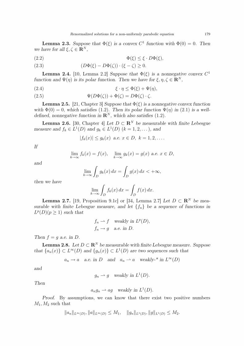
Lemma 2.3. Suppose that Φ(ξ) is a convex C1 function with Φ(0) = 0. Thenwe have for all ξ, ζ ∈ RN ,
Φ(ξ) ≤ ξ ·DΦ(ξ),(2.2)(DΦ(ξ)−DΦ(ζ)) · (ξ − ζ) ≥ 0.(2.3)
Lemma 2.4. [10, Lemma 2.2] Suppose that Φ(ξ) is a nonnegative convex C1
function and Ψ(η) is its polar function. Then we have for ξ, η, ζ ∈ RN ,
ξ · η ≤ Φ(ξ) + Ψ(η),(2.4)Ψ(DΦ(ζ)) + Φ(ζ) = DΦ(ζ) · ζ.(2.5)
Lemma 2.5. [21, Chapter 3] Suppose that Φ(ξ) is a nonnegative convex functionwith Φ(0) = 0, which satisfies (1.2). Then its polar function Ψ(η) in (2.1) is a well-defined, nonnegative function in RN , which also satisfies (1.2).
Lemma 2.6. [30, Chapter 4] Let D ⊂ RN be measurable with finite Lebesguemeasure and fk ∈ L1(D) and gk ∈ L1(D) (k = 1, 2, . . . ), and
|fk(x)| ≤ gk(x) a.e. x ∈ D, k = 1, 2, . . . .
Iflimk→∞
fk(x) = f(x), limk→∞
gk(x) = g(x) a.e. x ∈ D,
and
limk→∞
ˆ
D
gk(x) dx =
ˆ
D
g(x) dx < +∞,
then we have
limk→∞
ˆ
D
fk(x) dx =
ˆ
D
f(x) dx.
Lemma 2.7. [19, Proposition 9.1c] or [34, Lemma 2.7] Let D ⊂ RN be mea-surable with finite Lebesgue measure, and let fn be a sequence of functions inLp(D)(p ≥ 1) such that
fn f weakly in Lp(D),
fn → g a.e. in D.
Then f = g a.e. in D.
Lemma 2.8. Let D ⊂ RN be measurable with finite Lebesgue measure. Supposethat an(x) ⊂ L∞(D) and gn(x) ⊂ L1(D) are two sequences such that
an → a a.e. in D and an a weakly-* in L∞(D)
andgn g weakly in L1(D).
Thenangn ag weakly in L1(D).
Proof. By assumptions, we can know that there exist two positive numbersM1,M2 such that
‖an‖L∞(D), ‖a‖L∞(D) ≤ M1, ‖gn‖L1(D), ‖g‖L1(D) ≤ M2.
180 Chao Zhang and Shulin Zhou
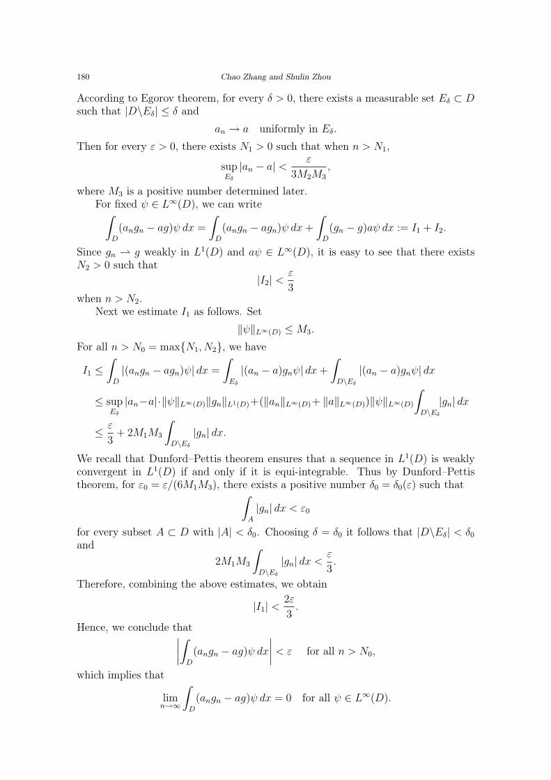
According to Egorov theorem, for every δ > 0, there exists a measurable set Eδ ⊂ Dsuch that |D\Eδ| ≤ δ and
an → a uniformly in Eδ.
Then for every ε > 0, there exists N1 > 0 such that when n > N1,
supEδ
|an − a| < ε
3M2M3
,
where M3 is a positive number determined later.For fixed ψ ∈ L∞(D), we can writeˆ
D
(angn − ag)ψ dx =
ˆ
D
(angn − agn)ψ dx +
ˆ
D
(gn − g)aψ dx := I1 + I2.
Since gn g weakly in L1(D) and aψ ∈ L∞(D), it is easy to see that there existsN2 > 0 such that
|I2| < ε
3when n > N2.
Next we estimate I1 as follows. Set
‖ψ‖L∞(D) ≤ M3.
For all n > N0 = maxN1, N2, we have
I1 ≤ˆ
D
|(angn − agn)ψ| dx =
ˆ
Eδ
|(an − a)gnψ| dx +
ˆ
D\Eδ
|(an − a)gnψ| dx
≤ supEδ
|an−a|·‖ψ‖L∞(D)‖gn‖L1(D)+(‖an‖L∞(D)+ ‖a‖L∞(D))‖ψ‖L∞(D)
ˆ
D\Eδ
|gn| dx
≤ ε
3+ 2M1M3
ˆ
D\Eδ
|gn| dx.
We recall that Dunford–Pettis theorem ensures that a sequence in L1(D) is weaklyconvergent in L1(D) if and only if it is equi-integrable. Thus by Dunford–Pettistheorem, for ε0 = ε/(6M1M3), there exists a positive number δ0 = δ0(ε) such thatˆ
A
|gn| dx < ε0
for every subset A ⊂ D with |A| < δ0. Choosing δ = δ0 it follows that |D\Eδ| < δ0
and2M1M3
ˆ
D\Eδ
|gn| dx <ε
3.
Therefore, combining the above estimates, we obtain
|I1| < 2ε
3.
Hence, we conclude that∣∣∣∣ˆ
D
(angn − ag)ψ dx
∣∣∣∣ < ε for all n > N0,
which implies that
limn→∞
ˆ
D
(angn − ag)ψ dx = 0 for all ψ ∈ L∞(D).
Renormalized solutions for a non-uniformly parabolic equation 181
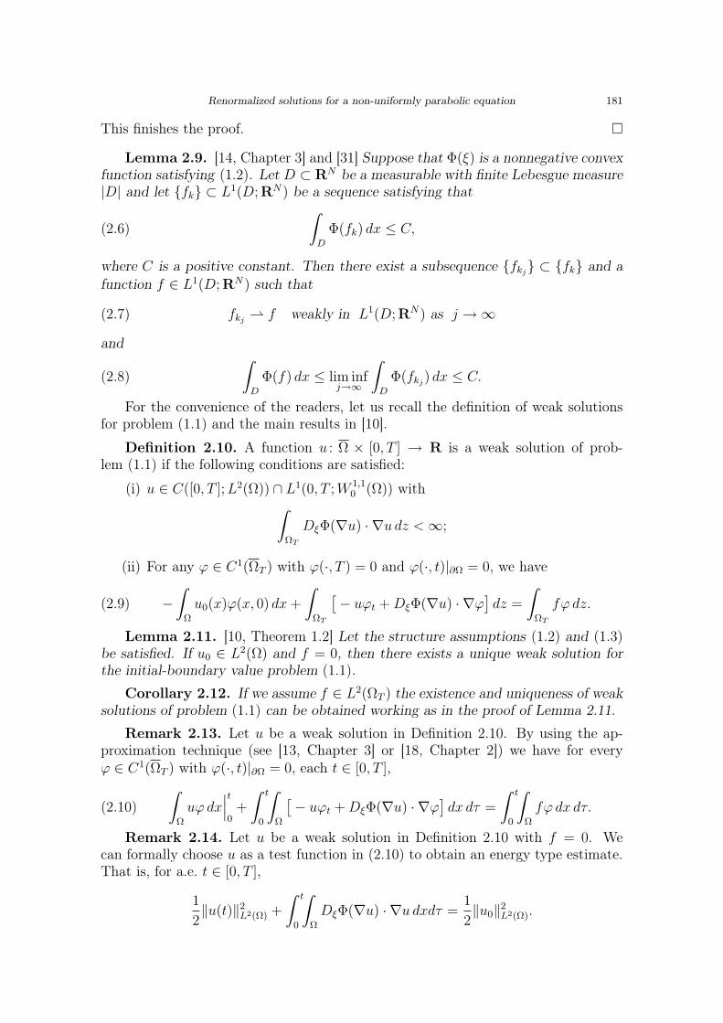
This finishes the proof. ¤
Lemma 2.9. [14, Chapter 3] and [31] Suppose that Φ(ξ) is a nonnegative convexfunction satisfying (1.2). Let D ⊂ RN be a measurable with finite Lebesgue measure|D| and let fk ⊂ L1(D;RN) be a sequence satisfying that
(2.6)ˆ
D
Φ(fk) dx ≤ C,
where C is a positive constant. Then there exist a subsequence fkj ⊂ fk and a
function f ∈ L1(D;RN) such that
(2.7) fkj f weakly in L1(D;RN) as j →∞
and
(2.8)ˆ
D
Φ(f) dx ≤ lim infj→∞
ˆ
D
Φ(fkj) dx ≤ C.
For the convenience of the readers, let us recall the definition of weak solutionsfor problem (1.1) and the main results in [10].
Definition 2.10. A function u : Ω × [0, T ] → R is a weak solution of prob-lem (1.1) if the following conditions are satisfied:
(i) u ∈ C([0, T ]; L2(Ω)) ∩ L1(0, T ; W 1,10 (Ω)) with
ˆ
ΩT
DξΦ(∇u) · ∇u dz < ∞;
(ii) For any ϕ ∈ C1(ΩT ) with ϕ(·, T ) = 0 and ϕ(·, t)|∂Ω = 0, we have
(2.9) −ˆ
Ω
u0(x)ϕ(x, 0) dx +
ˆ
ΩT
[− uϕt + DξΦ(∇u) · ∇ϕ]dz =
ˆ
ΩT
fϕ dz.
Lemma 2.11. [10, Theorem 1.2] Let the structure assumptions (1.2) and (1.3)be satisfied. If u0 ∈ L2(Ω) and f = 0, then there exists a unique weak solution forthe initial-boundary value problem (1.1).
Corollary 2.12. If we assume f ∈ L2(ΩT ) the existence and uniqueness of weaksolutions of problem (1.1) can be obtained working as in the proof of Lemma 2.11.
Remark 2.13. Let u be a weak solution in Definition 2.10. By using the ap-proximation technique (see [13, Chapter 3] or [18, Chapter 2]) we have for everyϕ ∈ C1(ΩT ) with ϕ(·, t)|∂Ω = 0, each t ∈ [0, T ],
(2.10)ˆ
Ω
uϕdx∣∣∣t
0+
ˆ t
0
ˆ
Ω
[− uϕt + DξΦ(∇u) · ∇ϕ]dx dτ =
ˆ t
0
ˆ
Ω
fϕ dx dτ.
Remark 2.14. Let u be a weak solution in Definition 2.10 with f = 0. Wecan formally choose u as a test function in (2.10) to obtain an energy type estimate.That is, for a.e. t ∈ [0, T ],
1
2‖u(t)‖2
L2(Ω) +
ˆ t
0
ˆ
Ω
DξΦ(∇u) · ∇u dxdτ =1
2‖u0‖2
L2(Ω).
182 Chao Zhang and Shulin Zhou
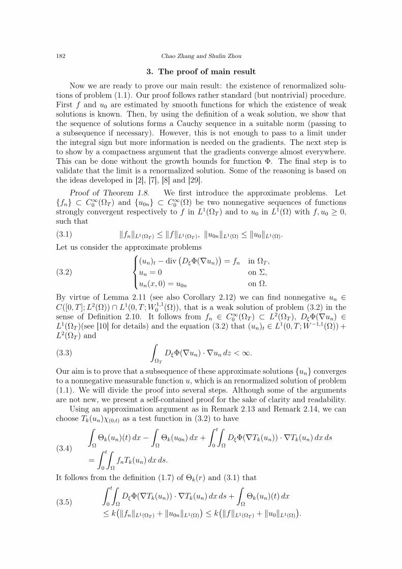
3. The proof of main result
Now we are ready to prove our main result: the existence of renormalized solu-tions of problem (1.1). Our proof follows rather standard (but nontrivial) procedure.First f and u0 are estimated by smooth functions for which the existence of weaksolutions is known. Then, by using the definition of a weak solution, we show thatthe sequence of solutions forms a Cauchy sequence in a suitable norm (passing toa subsequence if necessary). However, this is not enough to pass to a limit underthe integral sign but more information is needed on the gradients. The next step isto show by a compactness argument that the gradients converge almost everywhere.This can be done without the growth bounds for function Φ. The final step is tovalidate that the limit is a renormalized solution. Some of the reasoning is based onthe ideas developed in [2], [7], [8] and [29].
Proof of Theorem 1.8. We first introduce the approximate problems. Letfn ⊂ C∞
0 (ΩT ) and u0n ⊂ C∞0 (Ω) be two nonnegative sequences of functions
strongly convergent respectively to f in L1(ΩT ) and to u0 in L1(Ω) with f, u0 ≥ 0,such that
‖fn‖L1(ΩT ) ≤ ‖f‖L1(ΩT ), ‖u0n‖L1(Ω) ≤ ‖u0‖L1(Ω).(3.1)
Let us consider the approximate problems
(un)t − div(DξΦ(∇un)
)= fn in ΩT ,
un = 0 on Σ,
un(x, 0) = u0n on Ω.
(3.2)
By virtue of Lemma 2.11 (see also Corollary 2.12) we can find nonnegative un ∈C([0, T ]; L2(Ω)) ∩ L1(0, T ; W 1,1
0 (Ω)), that is a weak solution of problem (3.2) in thesense of Definition 2.10. It follows from fn ∈ C∞
0 (ΩT ) ⊂ L2(ΩT ), DξΦ(∇un) ∈L1(ΩT )(see [10] for details) and the equation (3.2) that (un)t ∈ L1(0, T ; W−1,1(Ω)) +L2(ΩT ) and
(3.3)ˆ
ΩT
DξΦ(∇un) · ∇un dz < ∞.
Our aim is to prove that a subsequence of these approximate solutions un convergesto a nonnegative measurable function u, which is an renormalized solution of problem(1.1). We will divide the proof into several steps. Although some of the argumentsare not new, we present a self-contained proof for the sake of clarity and readability.
Using an approximation argument as in Remark 2.13 and Remark 2.14, we canchoose Tk(un)χ(0,t) as a test function in (3.2) to have
ˆ
Ω
Θk(un)(t) dx−ˆ
Ω
Θk(u0n) dx +
ˆ t
0
ˆ
Ω
DξΦ(∇Tk(un)) · ∇Tk(un) dx ds
=
ˆ t
0
ˆ
Ω
fnTk(un) dx ds.
(3.4)
It follows from the definition (1.7) of Θk(r) and (3.1) thatˆ t
0
ˆ
Ω
DξΦ(∇Tk(un)) · ∇Tk(un) dx ds +
ˆ
Ω
Θk(un)(t) dx
≤ k(‖fn‖L1(ΩT ) + ‖u0n‖L1(Ω)
) ≤ k(‖f‖L1(ΩT ) + ‖u0‖L1(Ω)
).
(3.5)
Renormalized solutions for a non-uniformly parabolic equation 183
Recalling (2.2), we have
(3.6)ˆ
ΩT
Φ(∇Tk(un)) dz ≤ˆ
ΩT
DξΦ(Tk(∇un)) · ∇Tk(un) dz ≤ Ck,
which implies from (1.2) that
(3.7)ˆ
ΩT
|∇Tk(un)| dz ≤ C(k + 1),
that is Tk(un) is bounded in L1(0, T ; W 1,1
0 (Ω)).
If we choose k = 1 in the inequality (3.5), then for a.e. t ∈ [0, T ],ˆ
Ω
Θ1(un(t)) dx ≤ ‖f‖L1(ΩT ) + ‖u0‖L1(Ω).
Moreover,ˆ
Ω
|un(t)| dx ≤meas(Ω) + ‖f‖L1(ΩT ) + ‖u0‖L1(Ω).
Thus we obtain
(3.8) ‖un‖L∞(0,T ;L1(Ω)) ≤ C.
Step 1. We shall prove that un converges in C([0, T ]; L1(Ω)) and we shall finda subsequence which is almost everywhere convergent in ΩT .
Let m and n be two integers, then from (3.2) we can write the weak form asˆ T
0
〈(un − um)t, φ〉 dt +
ˆ
ΩT
[DξΦ(∇un)−DξΦ(∇um)] · ∇φ dz
=
ˆ
ΩT
(fn − fm)φ dz,
(3.9)
for all φ ∈ C10(ΩT ). Recalling (2.4), (2.5), (1.3) and (3.3), we observe that
|DξΦ(∇un) · ∇um| ≤ Φ(∇um) + Φ(−∇um) + Ψ(DξΦ(∇un))
≤ (C + 1)Φ(∇um) + DξΦ(∇un) · ∇un
≤ (C + 1)DξΦ(∇um) · ∇um + DξΦ(∇un) · ∇un ∈ L1(ΩT ).
Denote
(3.10) αn,m =
ˆ
ΩT
|fn − fm| dz +
ˆ
Ω
|u0n − u0m| dx.
We know thatlim
n,m→∞αn,m = 0.
Using an approximation argument as above, we conclude that w = T1(un − um)χ(0,t)
with t ≤ T can be a test function in (3.9). From (2.3), discarding the positive termwe get
ˆ
Ω
Θ1(un − um)(t) dx ≤ˆ
Ω
Θ1(u0n − u0m) dx + ‖fn − fm‖L1(ΩT )
≤ ‖u0n − u0m‖L1(Ω) + ‖fn − fm‖L1(ΩT ) = αn,m.
184 Chao Zhang and Shulin Zhou
Therefore, we conclude from the definition (1.7) of Θk(r) thatˆ
|un−um|<1
|un − um|2(t)2
dx +
ˆ
|un−um|≥1
|un − um|(t)2
dx
≤ˆ
Ω
[Θ1(un − um)](t) dx ≤ αn,m.
It follows from Hölder’s inequality thatˆ
Ω
|un − um|(t) dx =
ˆ
|un−um|<1|un − um|(t) dx +
ˆ
|un−um|≥1|un − um|(t) dx
≤(ˆ
|un−um|<1|un − um|2(t) dx
) 12
meas(Ω)12 + 2αn,m
≤ (2meas(Ω))12 α
12n,m + 2αn,m.
Thus we get‖un − um‖C([0,T ];L1(Ω)) → 0 as n,m →∞,
i.e., un is a Cauchy sequence in C([0, T ]; L1(Ω)). Then un converges to u inC([0, T ]; L1(Ω)). We find an a.e. convergent subsequence (still denoted by un)in ΩT such that
(3.11) un → u a.e. in ΩT .
Recalling (3.6) and Lemma 2.9, we may draw a subsequence (we also denote itby the original sequence for simplicity) such that
(3.12) ∇Tk(un) ηk weakly in L1(ΩT )
and ˆ
ΩT
Φ(ηk) dz ≤ Ck.
In view of (3.11), we conclude that ηk = ∇Tk(u) a.e. in ΩT .
Step 2. We shall prove that the sequence ∇un converges almost everywhere inΩT to ∇u (up to a subsequence).
We first claim that ∇un is a Cauchy sequence in measure. Let δ > 0, anddenote
E1 := (x, t) ∈ ΩT : |∇un| > h ∪ (x, t) ∈ ΩT : |∇um| > h,E2 := (x, t) ∈ ΩT : |un − um| > 1
and
E3 := (x, t) ∈ ΩT : |∇un| ≤ h, |∇um| ≤ h, |un − um| ≤ 1, |∇un −∇um| > δ,where h will be chosen later. It is obvious that
(x, t) ∈ ΩT : |∇un −∇um| > δ ⊂ E1 ∪ E2 ∪ E3.
For k ≥ 0, we can write
(x, t) ∈ ΩT : |∇un| ≥ h ⊂ (x, t) ∈ ΩT : |un| ≥ k ∪ (x, t) ∈ ΩT : |∇Tk(un)| ≥ h.Thus, applying (3.8), (1.2) and (3.7), there exist constants C > 0 such that
meas(x, t) ∈ ΩT : |∇un| ≥ h ≤ C
k+
Ck
h,
Renormalized solutions for a non-uniformly parabolic equation 185
when h is large appropriately. By choosing k = Ch12 , we deduce that
meas(x, t) ∈ ΩT : |∇un| ≥ h ≤ Ch−12 .
Let ε > 0. We may let h = h(ε) large enough such that
(3.13) meas(E1) ≤ ε/3 for all n,m ≥ 0.
On the other hand, by Step 1, we know that un is a Cauchy sequence in L1(ΩT ).Then there exists N1(ε) ∈ N such that
(3.14) meas(E2) ≤ ε/3 for all n, m ≥ N1(ε).
Moreover, since Φ is C1 and strictly convex, then from Lemma 2.2 and Defini-tion 2.1, there exists a real valued function m(h, δ) > 0 such that
(3.15) (DΦ(ξ)−DΦ(ζ)) · (ξ − ζ) ≥ m(h, δ) > 0
for all ξ, ζ ∈ RN with |ξ|, |ζ| ≤ h, |ξ − ζ| ≥ δ. By taking T1(un − um) as a testfunction in (3.9), we obtain
m(h, δ)meas(E3) ≤ˆ
E3
[DξΦ(∇un)−DξΦ(∇um)] · (∇un −∇um) dz
≤ˆ
ΩT
[DξΦ(∇un)−DξΦ(∇um)] · ∇T1(un − um) dz
≤ˆ
ΩT
|fn − fm| dz +
ˆ
Ω
|u0n − u0m| dx = αn,m,
which implies that
meas(E3) ≤ αn,m
m(h, δ)≤ ε/3,
for all n,m ≥ N2(ε, δ). It follows from (3.13) and (3.14) that
meas(x, t) ∈ ΩT : |∇un −∇um| > δ ≤ ε for all n,m ≥ maxN1, N2,that is ∇un is a Cauchy sequence in measure. Then we may choose a subsequence(denote it by the original sequence) such that
∇un → v a.e. in ΩT .
Thus, from Proposition 1.6 and ∇Tk(un) ∇Tk(u) weakly in L1(ΩT ), we deducefrom Lemma 2.7 that v coincides with the very weak gradient of u. Therefore, wehave
(3.16) ∇un → ∇u a.e. in ΩT .
Step 3. We shall prove that u is a renormalized solution.For given a, k > 0, define the function Tk,a(s) = Ta(s− Tk(s)) as
Tk,a(s) =
s− k sign(s) if k ≤ |s| < k + a,
a sign(s) if |s| ≥ k + a,
0 if |s| ≤ k.
186 Chao Zhang and Shulin Zhou
Using Tk,a(un) with un ≥ 0 as a test function in (3.2), we findˆ
|un|>kΘa(un − k)(T ) dx−
ˆ
|u0n|>kΘa(u0n − k) dx
+
ˆ
k≤|un|≤k+aDξΦ(∇un) · ∇un dz ≤
ˆ
Ω
fnTk,a(un) dz,
which yields thatˆ
k≤|un|≤k+aDξΦ(∇un) · ∇un dz ≤ a
(ˆ
|un|>k|fn| dz +
ˆ
|u0n|>k|u0n| dx
).
Recalling the fact that u belongs to C([0, T ]; L1(Ω)), we have
(3.17) limk→∞
meas(x, t) ∈ ΩT : |u| > k = 0.
Since DξΦ(∇un) · ∇un ≥ 0, by Fatou’s lemma, (3.11) and (3.16), we getˆ
k≤|u|≤k+aDξΦ(∇u) · ∇u dz =
ˆ
ΩT
DξΦ(∇u) · ∇uχk≤|u|≤k+a dz
=
ˆ
ΩT
lim infn→∞
DξΦ(∇un) · ∇unχk≤|un|≤k+a dz
≤ lim infn→∞
ˆ
k≤|un|≤k+aDξΦ(∇un) · ∇un dz.
Furthermore, sinceˆ
|un|>k|fn| dz =
ˆ
|un|>k|fn − f | dz +
ˆ
|un|>k|f | dz
≤ˆ
ΩT
|fn − f | dz +
ˆ
|un|>k|f | dz,
from (3.17) we have
limk→∞
limn→∞
ˆ
|un|>k|fn| dz = 0.
Similarly, we know
limk→∞
limn→∞
ˆ
|u0n|>k|u0n| dx = 0.
Therefore, passing to the limit first in n then in k, we conclude that
limk→∞
ˆ
(x,t)∈ΩT :k≤|u(x,t)|≤k+aDξΦ(∇u) · ∇u dz = 0.
Choosing a = 1, we obtain the renormalized condition, i.e.,
limk→∞
ˆ
(x,t)∈ΩT :k≤|u(x,t)|≤k+1DξΦ(∇u) · ∇u dz = 0.
Let S ∈ C∞(R+) be such that suppS ′ ⊂ [0,M ] for some M > 0. For everynonnegative function ϕ ∈ C∞(ΩT ) with ϕ(x, T ) = 0, S ′(un)ϕ is a test function in

Renormalized solutions for a non-uniformly parabolic equation 187
(3.2). It yieldsˆ
ΩT
∂S(un)
∂tϕ dz +
ˆ
ΩT
[S ′(un)DξΦ(∇un) · ∇ϕ
+ S ′′(un)DξΦ(∇un) · ∇unϕ] dz =
ˆ
ΩT
fnS′(un)ϕdz.
(3.18)
First we consider the first term on the left-hand side of (3.18). Since S is boundedand continuous, (3.11) implies that S(un) converges to S(u) a.e. in ΩT and weakly-*in L∞(ΩT ) . Then ∂S(un)
∂tconverges to ∂S(u)
∂tin D′(ΩT ) as n →∞, that is
ˆ
ΩT
∂S(un)
∂tϕ dz →
ˆ
ΩT
∂S(u)
∂tϕ dz.
For the other terms on the left-hand side of (3.18), because of suppS ′ ⊂ [0,M ]we know
S ′(un)DξΦ(∇un) = S ′(un)DξΦ(∇TM(un)).
Using (3.11) and S ∈ C∞(R+), we have
(3.19) S ′(un) → S ′(u) a.e. in ΩT .
In view of (3.5) and (2.5), we know thatˆ
ΩT
Ψ(DξΦ(∇TM(un))) dz ≤ C.
Applying Lemma 2.5, Lemma 2.9 and (3.12), we conclude that (up to a subsequence)
(3.20) DξΦ(∇TM(un)) DξΦ(∇TM(u)) weakly in L1(ΩT ).
Then (3.19), (3.20), the boundedness of S ′ and Lemma 2.8 yield that
S ′(un)DξΦ(∇Tm(un)) S ′(u)DξΦ(∇TM(u)) weakly in L1(ΩT ).
Noting thatS ′(u)DξΦ(∇u) = S ′(u)DξΦ(∇TM(u)),
we deduce thatˆ
ΩT
S ′(un)DξΦ(∇un) · ∇ϕdz →ˆ
ΩT
S ′(u)DξΦ(∇u) · ∇ϕdz,
as n →∞.Moreover, since S ′′(un) ≤ 0, ϕ ≥ 0 and
DξΦ(∇un) · ∇un ≥ 0,
then−S ′′(un)DξΦ(∇un) · ∇unϕ ≥ 0.
Thus from Fatou’s lemma, (3.11) and (3.16), we obtain that
−ˆ
ΩT
S ′′(u)DξΦ(∇u) · ∇uϕdz ≤ − lim infn→∞
ˆ
ΩT
S ′′(un)DξΦ(∇un) · ∇unϕdz.
188 Chao Zhang and Shulin Zhou
Using the strong convergence of fn, (3.11) and the Lebesgue dominated conver-gence theorem, we can pass to the limits as n →∞ for the right-hand side of (3.18)to conclude that
−ˆ
Ω
S(u0)ϕ(x, 0) dx−ˆ T
0
ˆ
Ω
S(u)∂ϕ
∂tdz
+
ˆ T
0
ˆ
Ω
[S ′(u)DξΦ(∇u) · ∇ϕ + S ′′(u)DξΦ(∇u) · ∇uϕ] dz
≥ˆ T
0
ˆ
Ω
fS ′(u)ϕdz
for all k > 0 and ϕ ∈ C1(ΩT ) with ϕ ≥ 0 and ϕ|Σ = 0. This finishes the proof. ¤Acknowledgements. The authors wish to thank the anonymous referee for careful
reading of the early version of this manuscript and bringing several reference papersto their attention and providing many valuable suggestions and comments. The firstauthor was supported by Hei Long Jiang Postdoctoral Foundation and the NaturalScientific Research Innovation Foundation in Harbin Institute of Technology. Thesecond author was supported in part by the NSFC under Grant 10990013.
References
[1] Acerbi, E., and N. Fusco: A regularity theorem for minimizers of quasi-convex integrals. -Arch. Ration. Mech. Anal. 99, 1987, 261–281.
[2] Bénilan, P., L. Boccardo, T. Gallouët, R. Gariepy, M. Pierre, and J. L. Vazquez:An L1-theory of existence and uniqueness of solutions of nonlinear elliptic equations. - Ann.Sc. Norm. Super. Pisa Cl. Sci. (4) 22, 1995, 241–273.
[3] Blanchard, D., and F. Murat: Renormalised solutions of nonlinear parabolic problemswith L1 data: Existence and uniqueness. - Proc. Roy. Soc. Edinburgh Sect. A 127:6, 1997,1137–1152.
[4] Blanchard, D., F. Murat, and H. Redwane: Existence and uniqueness of a renormalizedsolution for a fairly general class of nonlinear parabolic problems. - J. Differential Equations177:2, 2001, 331–374.
[5] Blanchard, D., and H. Redwane: Renormalized solutions for a class of nonlinear evolutionproblems. - J. Math. Pures Appl. (9) 77, 1998, 117–151.
[6] Boccardo, L., A. Dall’Aglio, T. Gallouët, and L. Orsina: Nonlinear parabolic equa-tions with measure data. - J. Funct. Anal. 147:1, 1997, 237–258.
[7] Boccardo, L., and T. Gallouët: Nonlinear elliptic and parabolic equations involving mea-sure data. - J. Funct. Anal. 87:1 ,1989, 149–169.
[8] Boccardo. L., andT. Gallouët: Nonlinear elliptic equations with right-hand side measures.- Comm. Partial Differential Equations 17:3-4, 1992, 641–655.
[9] Boccardo, L., D. Giachetti, J. I. Diaz, and F. Murat: Existence and regularity ofrenormalized solutions for some elliptic problems involving derivations of nonlinear terms. - J.Differential Equations 106, 1993, 215–237.
[10] Cai, Y., and S. Zhou: Existence and uniqueness of weak solutions for a non-uniformly para-bolic equation. - J. Funct. Anal. 257, 2009, 3021–3042.
[11] Cellina, A.: On the validity of the Euler–Lagrange equation. - J. Differential Equations 171,2001, 430–442.
[12] Chapman, S., and T.G. Cowling: Mathematical theory of nonuniform gases. - CambridgeUniv. Press, 3rd edition, 1990.
Renormalized solutions for a non-uniformly parabolic equation 189
[13] Chen, Y.: Parabolic partial differential equations of second order. - Peking Univ. Press, Bei-jing, 2003 (in Chinese).
[14] Dacorogna, B.: Direct methods in the caculus of variations. - Springer-Verlg, Berlin-Heidelberg, 1989.
[15] Dal Maso, G., F. Murat, L. Orsina, and A. Prignet: Renormalized solutions of ellipticequations with general measure data. - Ann. Sc. Norm. Super. Pisa Cl. Sci. (4) 28:4, 1999,741–808.
[16] Dall’Aglio, A.: Approximated solutions of equations with L1 data. Application to the H-convergence of quasi-linear parabolic equations. - Ann. Mat. Pura Appl. (4) 170, 1996, 207–240.
[17] Duc, D.M., and J. Eells: Regularity of exponetional harmonic functions. - Internat. J.Math. 2, 1991, 395–408.
[18] DiBenedetto, E.: Degenerate parabolic equations. - Springer-Verlag, Berlin, 1993.
[19] DiBenedetto, E.: Real analysis. - Birkhäuser, Boston, 2002.
[20] DiPerna, R. J., and P.-L. Lions: On the Cauchy problem for Bolzmann equations: globalexistence and weak stability. - Ann. of Math. (2) 130:2, 1989, 321–336.
[21] Evans, L. C.: Partial differential equations. - Amer. Math. Soc., Providence, Rhode Island,1998.
[22] Fuchs, M., and G. Mingione: Full C1,α-regularity for free and contrained local minimizersof elliptic variational integrals with nearly linear growth. - Manuscripta Math. 102:2, 2000,227–250.
[23] Hiriart-Urruty, J.-B., and C. Lemaréchal: Fundamentals of convex analysis. - Springer-Verlag, Berlin-Heidelberg, 2001.
[24] Lieberman, G.M.: On the regularity of the minimizer of a functional with exponetial growth.- Comment. Math. Univ. Carolin. 33:1, 1992, 45–49.
[25] Lions, J.-L.: Quelques méthodes de résolution des problèmes aux limites non linéaire. - Dunodet Gauthier-Villars, Paris, 1969.
[26] Lions, P.-L.: Mathematical topics in fluid mechanics, Vol. 1: Incompressible models. - OxfordUniv. Press, Oxford, 1996.
[27] Lions, P.-L., and F. Murat: Solutions renormalisées d’équations elliptiques non linéaires. -Unpublished.
[28] Naito, H.: On a local Hölder continuity for a minimizer of the exponential energy functinal.- Nagoya Math. J. 129, 1993, 97–113.
[29] Prignet, A.: Existence and uniqueness of “entropy” solutions of parabolic problems with L1
data. - Nonlinear Anal. 28:12, 1997, 1943–1954.
[30] Royden, H. L.: Real analysis. - Macmillan Company, New York, 2nd edition, 1968.
[31] Saadoune, M., and M. Valadier: Extraction of a “good” subsequence from a boundedsequence of integrable functions. - J. Convex Anal. 2, 1995, 345–357.
[32] Serrin, J.: Pathological solutions of elliptic differential equations. - Ann. Sc. Norm. Super.Pisa Cl. Sci. (3) 18, 1964, 385–387.
[33] Zhang, C., and S. Zhou: Renormalized and entropy solutions for nonlinear parabolic equa-tions with variable exponents and L1 data. - J. Differential Equations 248:6, 2010, 1376–1400.
[34] Zhang, C., and S. Zhou: Entropy solutions for a non-uniformly parabolic equation. -Manuscripta Math. 131:3-4, 2010, 335–354.
Received 18 March 2011Revised received 18 July 2011