RESOLUTION OF SINGULARITIESIN POSITIVE CHARACTERISTICS

HEISUKE HIRONAKA

TO WAKA

Abstract. A proof of resolution of singularities in characteristicp > 0 and all dimensions.

Contents

1. Introduction 31.1. Acknowledgments. 42. Preliminaries 42.1. Ideal exponents 42.2. Normal crossing data 52.3. Infinitely near singularities S(E) 53. Three results for basic E-operations: Diff, AR, NE 73.1. Differentiation Theorem 73.2. Ambient reductions 103.3. Numerical exponent theorem connecting geometric S and

algebraic ℘ 124. Characteristic algebra ℘(E) 164.1. Edge data of ℘(E) 184.2. Cotangent module cot(E) 224.3. Edge Decomposition Theorem. 245. The negative degree part of ℘(E). 256. Base-hikes and core-focusing of E 296.1. Maximum base-hike E 296.2. Core focusing E 306.3. Coherent LL-heads module L(E) 337. Permissible transformations and effects on ℘(E) 357.1. Effects on edge data of ℘(E) 357.2. The rule of transformation of ℘nega 367.3. Rule of transformation for ℘nega 397.4. Coordinate translation in p > 0 39

Date: March 23, 2017.1

2 H. HIRONAKA

7.5. Cleaning by edge equation g = yq + ε 408. Standard unit-monomial expression 428.1. Finiteness of unit-monomial sum expression 428.2. Frobenius filtration with unit-monomials 468.3. Standard expressions for ε = g − yq 468.4. Cleaned standard expressions for ε = g − yq 469. Local Leverage-up Exponent-down (LLUED) 469.1. Master keys for the existence of LLUED 479.2. Introductory comments on local vs global IUED conceots 479.3. Frontier symbols of a standard expression 489.4. Frontier symbolics 499.5. Differentiation-product H[-operator 509.6. H[-operators for LLUED 509.7. Local H[ case by case 519.8. LL-heads and LL-tails of LL-chains 549.9. LL-chains headed by L(E, q) 549.10. LLED propagation from a point to a neighborhood 569.11. Linear combinations of LL-chains 5810. LL-chains modifications 5910.1. Enclosure of Sing(E) by LL-tails 6011. Coordinate-free LL-chains and LL-tails 6111.1. Symbolic power and degree change 6111.2. Abstract LL-chains with ℘nega 6211.3. Λ and τ operators 6312. GLUED: the globalization of LLUED 6412.1. Define the step down operator σ on L-levels 6613. The global coherent GLUED-chain diagram 6713.1. Define T(E) and Cot(E) 6714. Local LL-chains vs global GLUED-diagram 6814.1. Rule of transformation of T(E) 7014.2. Cotangent AR-heading 7014.3. How large `� e should be? 7114.4. LLAR-type generators of T 7315. AR-schemes and AR-reductions 7415.1. AR-schemes tied with GLUED-tails 7515.2. Iteration of ambient reduction of AR-scheme 7815.3. Terminal Y and terminal plat 7916. PROOF of RESOLUTION of SINGULARITIES, p > 0 8116.1. Theorem ∆ and Γ-monomials 8116.2. Theorem ∇ I: Domino-falls by ∇ blowups 8416.3. Theorems ∇ II-III: Inductive proof of resolution 8716.4. Θ(E) headed by σL(E) 87

SINGULARITIES 3

17. Comments on the methodology of this paper 89References 90

1. Introduction

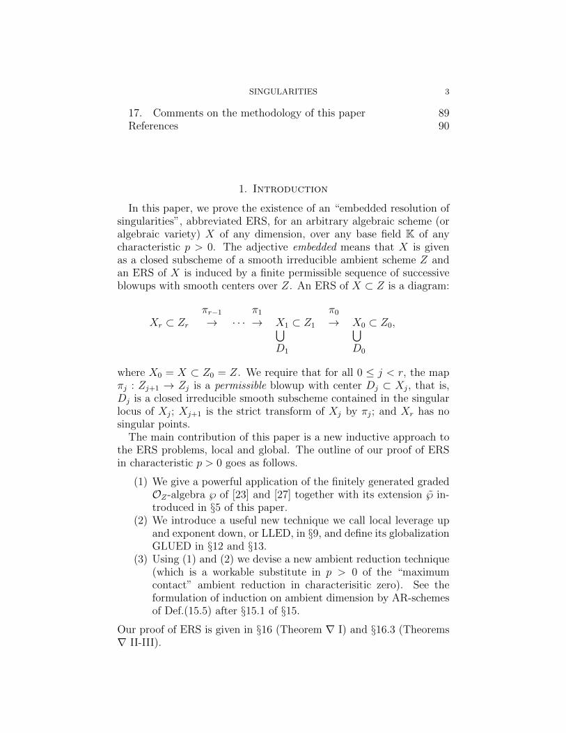
In this paper, we prove the existence of an “embedded resolution ofsingularities”, abbreviated ERS, for an arbitrary algebraic scheme (oralgebraic variety) X of any dimension, over any base field K of anycharacteristic p > 0. The adjective embedded means that X is givenas a closed subscheme of a smooth irreducible ambient scheme Z andan ERS of X is induced by a finite permissible sequence of successiveblowups with smooth centers over Z. An ERS of X ⊂ Z is a diagram:

Xr ⊂ Zr

πr−1

→ · · ·π1

→ X1 ⊂ Z1⋃D1

π0

→ X0 ⊂ Z0,⋃D0

where X0 = X ⊂ Z0 = Z. We require that for all 0 ≤ j < r, the mapπj : Zj+1 → Zj is a permissible blowup with center Dj ⊂ Xj, that is,Dj is a closed irreducible smooth subscheme contained in the singularlocus of Xj; Xj+1 is the strict transform of Xj by πj; and Xr has nosingular points.

The main contribution of this paper is a new inductive approach tothe ERS problems, local and global. The outline of our proof of ERSin characteristic p > 0 goes as follows.

(1) We give a powerful application of the finitely generated gradedOZ-algebra ℘ of [23] and [27] together with its extension ℘ in-troduced in §5 of this paper.

(2) We introduce a useful new technique we call local leverage upand exponent down, or LLED, in §9, and define its globalizationGLUED in §12 and §13.

(3) Using (1) and (2) we devise a new ambient reduction technique(which is a workable substitute in p > 0 of the “maximumcontact” ambient reduction in characterisitic zero). See theformulation of induction on ambient dimension by AR-schemesof Def.(15.5) after §15.1 of §15.

Our proof of ERS is given in §16 (Theorem ∇ I) and §16.3 (Theorems∇ II-III).

4 H. HIRONAKA

1.1. Acknowledgments. I received invaluable mathematical influenceand guidance from numerous excellent mathematical teachers and col-leagues in the course of completing this work. I have been indebted somuch and for so long to many mathematical seniors, first and foremostto my teachers Oscar Zariski, Masayoshi Nagata, Alexander Grothendiekand Shreeram Abhyankar. I must also mention the valuable influenceand stimulation I have received from my colleagues Michael Artin,David Mumford, Bernard Teissier, Le Dung Trang, S-Moh, Jose-ManuelAroca, Mark Spivakowski, U.O. Villamayor, Herwig Hauser, HirakuKawanoue, June-E and many other algebraic geometers with stronginterests in the topics surrounding singularities. Finally, I am gratefulfor the constant continuous encouragement, and multiple proof-readingand misprints-checking by Woo Yang Lee of Seoul National Universityand Tadao Oda of Tohoku University during the past decade of earnestbut slow research toward the proof of resolution of singularities in pos-itive characteristics and for all dimensions.

2. Preliminaries

In this section, we review some of the basic definitions used through-out this paper: the ideal exponent (§2.1), normal crossing data (§2.2),and infinitely near singularities (§2.3).

Throughout this paper an ambient scheme Z always means a smoothirreducible scheme of finite type defined over a perfect base field K ofcharacteristic p > 0. In particular we may choose K = Z/pZ.

Let OZ denote the structure sheaf of Z. We may write O for OZ andOξ for the local ring OZ,ξ at a point ξ ∈ Z. Sometimes the notationRξ or R for OZ,ξ and Mξ or M for the maximal ideal max(Oξ) of Oξare used. We write κξ or κ for the residue field Rξ/Mξ. The symbol ρdenotes the Frobenius endomorphism, sending each element to its p-thpower. It gives the filtration

O ⊃ ρ(O) ⊃ ρ2(O) ⊃ · · ·

where each ρi(O) is a locally free ρj(O)-module for j > i. It is fre-quently used for polynomial approximations and differentiations in O.Denote by Ycl the set of closed points of a scheme Y .

2.1. Ideal exponents. For an ideal exponent E = (J, b) we writeSing(E) for the singular locus of E which is a closed reduced subschemeof Z consisting of those points ξ with ordξJ ≥ b. A blowup π : Z ′ → Zwith center D is said to be permissible for E if D is a closed smoothirreducible subscheme of Sing(E).

SINGULARITIES 5

Definition 2.1. The transform E ′ of E by π is E ′ = (J ′, b) in Z ′ withJOZ′ = I(D)bJ ′OZ′ where I(D) denotes the ideal of D in OZ .

Note that I(D)OZ′ is a locally everywhere nonzero principal idealwhose b-power divides JOZ′ thanks to the permissibility of π for (J, b).

Definition 2.2. The following graded algebras will be used frequentlyin this paper.

(1) Blposi(Z) =⊕

i>0Bl(Z, i) and Blnega(Z) =⊕

j<0Bl(Z, j)

where, Bl(Z, j) = O for all integers j;(2) Bl(Z)◦ = Blposi(Z)

⊕O;

(3) Bl(Z) = Blposi(Z)⊕O⊕

Blnega(Z); and(4) for blξ(Z, j) = (Mξ)

j and ξ ∈ Zcl,

blξ(Z) =⊕j≥0

blξ(Z, j)

⊂⊕j∈Z

Bl(Z, j) = Bl(Z).

It should be noted that Bl(Z) has positive part as well as negativepart in homogeneity, unlike blξ(Z). We have the natural epimorphism

blξ(Z) → grξ(Z) = grmax(Oξ)(Oξ) =⊕

j≥0(Mξ)j/(Mξ)

j+1(1)

whose kernel is Mξblξ(Z) = max(Oξ)blξ(Z).

2.2. Normal crossing data. We will be working with normal cross-ing data, NC-data for short, using the notation Γ = (Γ1, · · · ,Γs) whereeach Γi is a normal crossing smooth irreducible hypersurface in Z.(Some Γi may be empty and even the system may be empty to beginwith.)

Definition 2.3. A blowup π : Z ′ → Z is said to be permissible for Γif its center D has normal crossing with Γ. The transform Γ′ of Γ by πis defined to be Γ′ = (Γ′1, · · · ,Γ′s,Γ′s+1) where Γ′i is the strict transformof Γi by π for every i ≤ s and Γ′s+1 = π−1(D) is the exceptional divisorof π.

Note that the strict transform Y ′ of any Y ⊂ D becomes empty butthe information is kept in Γ′ as the new exceptional divisor Γ′s+1.

2.3. Infinitely near singularities S(E). There are many differentdefinitions for infinitely near singular points, one by pointed arcs andanother by blowups. In this paper we choose the one given in [23],which we review here.

6 H. HIRONAKA

Definition 2.4. An LSB (finite sequence of localized smooth blowups)over Z means any diagram as follows.

Zr

πr−1

→ Ur−1 ⊂ Zr−1⋃Dr−1

πr−2

→ · · ·π1

→ U1 ⊂ Z1⋃D1

π0

→ U0 ⊂ Z0 = Z⋃D0

where Ui ⊂ Zi is open, Di is a smooth (or only regular) irreducibleclosed in Ui and the πi : Zi+1 → Ui is the blow-up with center Di.

Definition 2.5. We define the t-indexed disjoint union with arbitraryfinite systems of indeterminates t, and write it symbolically as follows.

S(E) =⋃t

{the LSBs over Z[t] permissible for E[t] = (J [t], b)

}called the totality of the infinitely near singularities of E in Z.

Remark 2.6. Permissibility of LSB for E implies that the transformEi of E in Zi is well defined and Sing(Ei) is then equal to the unionof the images of the centers of all the permissible sequences of blowupsthat can follows. As a matter of fact we lose nothing by replacingZj ⊃ Sing(Ei) by the germ of Ei in all of the steps. It is important toinclude those ambient extensions Z to Z[t]. By using the extensions thedefinition dramatically advances its significance in an essential manner.

Remark 2.7 (Notational warning (2)). In this paper we make thefollowing change of notation from the original source [23]:

(2) for all i, ℘(E, i) replaces Jmax(E, i).

Consider an ideal exponent E = (J, b), where J is the coherent idealJ 6= (0) in OZ and an integer b, positive to begin with. The ℘(E) =⊕

j≥0 ℘(E, j) is a finitely generated graded algebra where each homoge-

nous part ℘(E, j) is a coherent ideal in OZ for every degree j ≥ 0. Itwas introduced in [23] (with the slight change in notation mentionedabove).

We have been using the notation ℘(E) =⊕

i≥0 Jmax(E, i) in relationto Th.(4.1) of §4, while referring to results in [23]. The symbol ℘ isconvenient, since we will work with an extension of ℘ that includesthe negative parts ℘nega(E, i),∀i < 0 (see §5). As to the characteristicnature of ℘, in particular for the elements of the negative parts ℘nega,we will take special care to explian

(1) the rule of transformation by blowups permissible for E; and(2) the meaning of multiplications and differentiations.

SINGULARITIES 7

3. Three results for basic E-operations: Diff, AR, NE

We review three key technical theorems involving the operations Dif-ferentiation down Diff, Ambient resolution AR and numerical expo-nents NE originally proved in [22] and [24]. These play an importantrole in studying the characteristic algebra and its relations with thetheory of infinitely near singularities (see §4).

In this section we do not assume that the base field K is perfect.However we assume that the ambient scheme Z is smooth over K andthus it remains so under any base field extension.

3.1. Differentiation Theorem. The following theorem was originallyproved in [22] and [24], and is an important tool for the proofs thatfollow in later sections.

Theorem 3.1 (Differentiation theorem). For every OZ-submodule Dof Diff

(i)Z , we have S(DJ, b− i) ⊃ S(J, b).

In what follows we review some known results on differential opera-tors, especially in the case of a perfect base field of characteristic p > 0.There are substantial differences in properties of differentiation fromthe characteristic zero case. For example, in p > 0, anti-differentiationis not well-defined, and hence the Weierstrass preparation theorem cannot be used in inductions on dimensions or on the number of variables.A crucial point for our proof of ERS is that differential operators can,with the help of Frobenius p-th powers, be quite useful in an inductivetreatment of singularities, but for this we need dramatically differenttechniques as we explain.

3.1.1. Definition of differential operators in p > 0. Write O for OZ .

We define the O-module Diff(m)Z of differential operators of orders ≤ m

in O, which is identified with the O-module of differentials D(m).

DK(m) = HomO

(DK

(m),O), ∀m ≥ 0(3)

where DK(m) =

(O ⊗K O

)/∆K

m+1 for the diagonal ideal ∆K, in which

the DK(m) is a coherent O-module by the action of O on the left factor

of the tensor product. Every element ∂ ∈ DK(m) determines the action

on every f ∈ O in the following manner.

(4) f 7→ 1⊗ f 7→ ∂(1⊗ f) 7→ ∂(f) ∈ Owhere ∂(1⊗f) 7→ ∂(f) denotes the identity map which is the definitionof ∂(f). It is then better to say that ∂ is the map f 7→ ∂(f). Withthis K-automorphic action in O induced by ∂ is called a differentialoperator of order ≤ m. The O-module of those differential operators

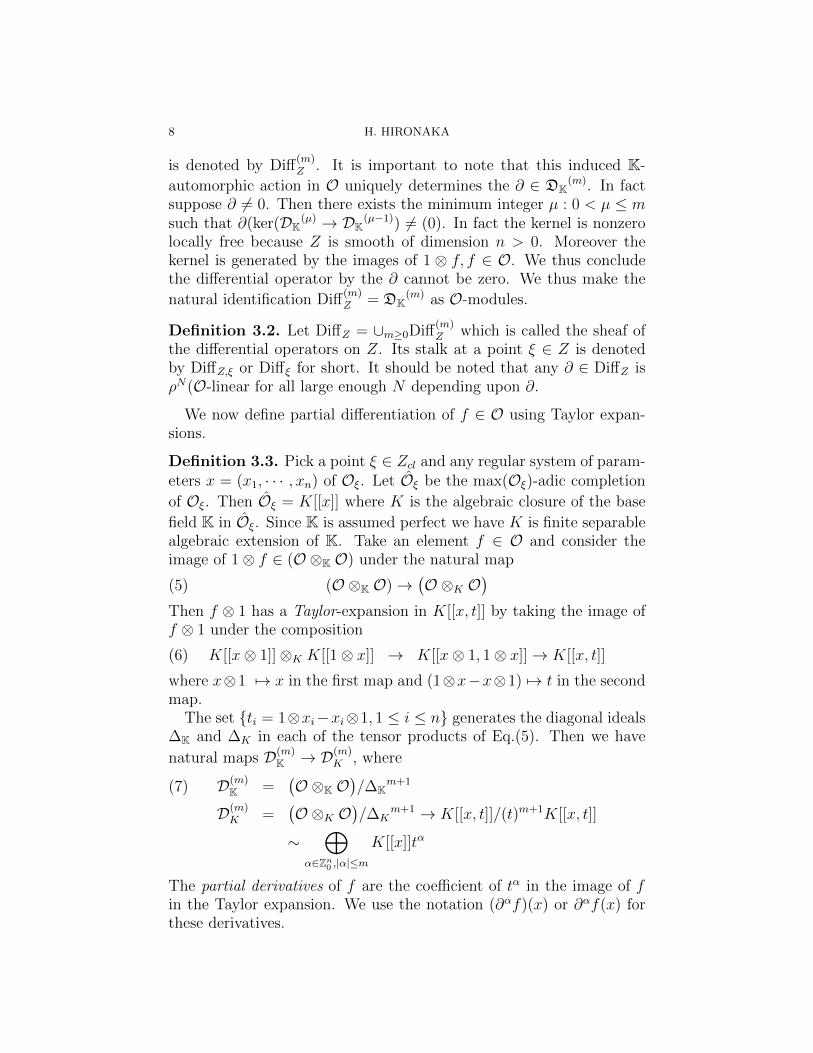
8 H. HIRONAKA

is denoted by Diff(m)Z . It is important to note that this induced K-

automorphic action in O uniquely determines the ∂ ∈ DK(m). In fact

suppose ∂ 6= 0. Then there exists the minimum integer µ : 0 < µ ≤ msuch that ∂(ker(DK

(µ) → DK(µ−1)) 6= (0). In fact the kernel is nonzero

locally free because Z is smooth of dimension n > 0. Moreover thekernel is generated by the images of 1 ⊗ f, f ∈ O. We thus concludethe differential operator by the ∂ cannot be zero. We thus make the

natural identification Diff(m)Z = DK

(m) as O-modules.

Definition 3.2. Let DiffZ = ∪m≥0Diff(m)Z which is called the sheaf of

the differential operators on Z. Its stalk at a point ξ ∈ Z is denotedby DiffZ,ξ or Diffξ for short. It should be noted that any ∂ ∈ DiffZ isρN(O-linear for all large enough N depending upon ∂.

We now define partial differentiation of f ∈ O using Taylor expan-sions.

Definition 3.3. Pick a point ξ ∈ Zcl and any regular system of param-eters x = (x1, · · · , xn) of Oξ. Let Oξ be the max(Oξ)-adic completion

of Oξ. Then Oξ = K[[x]] where K is the algebraic closure of the base

field K in Oξ. Since K is assumed perfect we have K is finite separablealgebraic extension of K. Take an element f ∈ O and consider theimage of 1⊗ f ∈ (O ⊗K O) under the natural map

(O ⊗K O)→(O ⊗K O

)(5)

Then f ⊗ 1 has a Taylor-expansion in K[[x, t]] by taking the image off ⊗ 1 under the composition

K[[x⊗ 1]]⊗K K[[1⊗ x]] → K[[x⊗ 1, 1⊗ x]]→ K[[x, t]](6)

where x⊗1 7→ x in the first map and (1⊗x−x⊗1) 7→ t in the secondmap.

The set {ti = 1⊗xi−xi⊗1, 1 ≤ i ≤ n} generates the diagonal ideals∆K and ∆K in each of the tensor products of Eq.(5). Then we have

natural maps D(m)K → D(m)

K , where

D(m)K =

(O ⊗K O

)/∆K

m+1(7)

D(m)K =

(O ⊗K O

)/∆K

m+1 → K[[x, t]]/(t)m+1K[[x, t]]

∼⊕

α∈Zn0 ,|α|≤m

K[[x]]tα

The partial derivatives of f are the coefficient of tα in the image of fin the Taylor expansion. We use the notation (∂αf)(x) or ∂αf(x) forthese derivatives.

SINGULARITIES 9

Note that we have the following fact.

Lemma 3.4. Every element of the form h⊗ 1−1⊗ h with h ∈ K ⊃ Khas zero class in the tensor product O ⊗K O/∆K

m+1. In other words

we claim that the natural homomorphism D(m)K[x] → D

(m)K[x] of Eq.(7) is in

fact an isomorphism for every m > 0.

Proof. For every integer ` � m we have g ∈ K such that ρ`(g) = h.Hence h⊗ 1 − 1⊗ h is equal to ρ`

(g ⊗ 1 − 1⊗ g

)which is in ∆K

m+1

with the diagonal ideal ∆K of O ⊗K O. Hence h⊗ 1 − 1⊗ h has zero

image in D(m)K[x] mod ∆m+1

K . �

Remark 3.5. Recall Eq.(7) following after Eq.(6) and then note that

1⊗ xβ = (1⊗ x)β 7→((x⊗ 1) + t

)β=∑

β∈γ+Zn0

(βγ

)xβ−γtγ

to which the action of HomOξ(·,Oξ) apples only to the tγ’s individuallyarbitrarily. In particular the differential operator ∂α sends tα 7→ 1 andtγ 7→ 0 for all γ 6= α. Locally at ξ ∈ Zcl there exists a free basis{∂a = ∂ax, a ∈ Zn0} of the Oξ-module DiffZ,ξ. They are well defined bythe following equality.

∂αxβ =

{(βα

)xβ−α if β ∈ α + Zn0

0 if otherwise(8)

Another way to have the same is by using a dummy variable t for x asfollows.

(9) (x+ t)β =∑

β:α∈α+Zn0

(∂αxβ)tα

3.1.2. Cartier operations, extension and contraction.

Lemma 3.6. Pick e ≥ 1 and let q = pe. Then with respect to thegiven x we can extend every σ ∈ Diffρe(Oξ)/K to ∂ ∈ DiffOξ/K suchthat the following condition is satisfied. Namely for all α ∈ Zn0 with0 ≤ αi < q,∀i, and for all hα ∈ ρe(Oξ), we have

∂(∑

α

xαhα

)=

∑α

xασ(hα) for all hα ∈ ρe(Oξ).(10)

In particular we have ∂(xα) = 0 for even α as above.

Proof. With the indeterminate copy t of x we examine the expansionin terms of t of (x + t)α × (hq)(x + t) for each h ∈ Oξ. The onlysummands of its monomial terms divisible by any factor of the kindta, where 0 ≤ ai < q for all i, must have a = (0). Hence ∂(xαhq)must be xασ(hq). Moreover {ta : 0 ≤ ai < q,∀i} are ρe(Oξ)-linearlyindependent. �

10 H. HIRONAKA

Definition 3.7. Following Lem.(3.6) ∂ will be called the x-Cartierextension of σ from Diffρe(Oξ)/K to DiffOξ/K.

Remark 3.8. (Agreement on elementary differential operators.)We agree that if x is chosen and fixed then every extension of elemen-tary differential operators from Diffρ`(Rξ)/K to DiffRξ/K will be alwaysassumed to be x-Cartier in the sense of Def.(3.7).

Definition 3.9. In contrast to the x-Cartier extension Def.(3.7), whichdepends on the choice of the coordinate system x, we have Cartier con-traction from DiffO down into Diffρ`(O) which is defined and denoted by

ρ` as follows.

∂ ∈ DiffO 7→ ρ`(∂) ∈ Diffρ`(O)(11)

where ρ`(∂)(fp`) = ∂(f)p

`for all f ∈ O. This Cartier contraction is

independent of local coordinate systems.

3.2. Ambient reductions. Cutting down the ambient dimension bytaking sections of the given singularity data is a useful technique forproving many theorems using induction on the dimension of the ambi-ent scheme. Hence it is important to investigate AR-techniques espe-cially for resolution of singularities.

Ambient reduction is explicitly performed by taking differentiationsin the normal direction along the smooth subscheme Y ⊂ Z. Theequivalent reduction is also done by taking all differentiations insteadof only normal differentiations because ℘-algebras are invariant by anydifferentiations before and after AR in the manner of the Diff-theoremTh.(3.1). Below is an explicit definition of AR by differentiations ofthe given ideal of E and any choice of local coordinate system.

Theorem 3.10. (Ambient Reduction Theorem) Given an ideal expo-nent E = (J, b) in Z we define

J ] =b−1∑j=0

(Diff

(j)Z J) b]

b−jwith b] = b!.

For every smooth subscheme W ⊂ Z we let F = (J ]OW , b]). ThenF is an ambient reduction of E from Z to W in the following sense:Pick any t and any LSB over Z[t] such that all of its centers are in thestrict transforms of W [t]. Then we have the LSB ∈ S(E) if and onlyif the LSB induces the one to W which belongs to S(F ).

3.2.1. AR in terms of S. For any smooth closed subscheme Y in anopen subset V ⊂ Z and for any ideal exponent F in V we have theambient reduction F (Y ) of F |V from V to Y where F |V dnotes the

SINGULARITIES 11

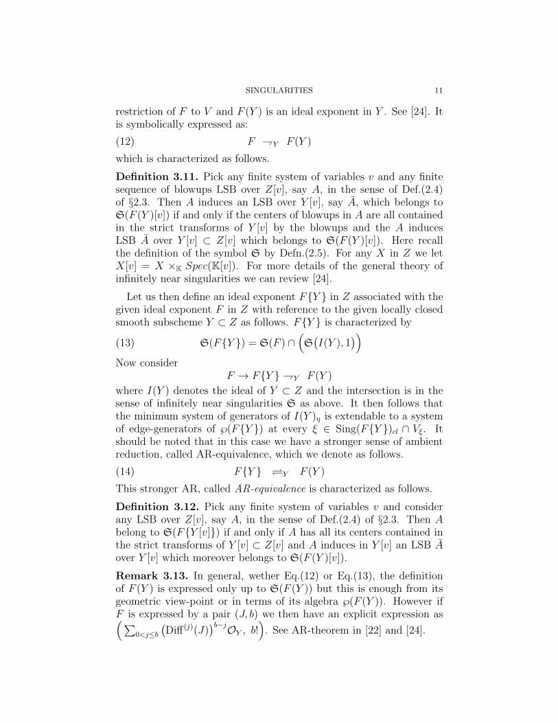
restriction of F to V and F (Y ) is an ideal exponent in Y . See [24]. Itis symbolically expressed as:

(12) F ⇁Y F (Y )

which is characterized as follows.

Definition 3.11. Pick any finite system of variables v and any finitesequence of blowups LSB over Z[v], say A, in the sense of Def.(2.4)of §2.3. Then A induces an LSB over Y [v], say A, which belongs toS(F (Y )[v]) if and only if the centers of blowups in A are all containedin the strict transforms of Y [v] by the blowups and the A inducesLSB A over Y [v] ⊂ Z[v] which belongs to S(F (Y )[v]). Here recallthe definition of the symbol S by Defn.(2.5). For any X in Z we letX[v] = X ×K Spec(K[v]). For more details of the general theory ofinfinitely near singularities we can review [24].

Let us then define an ideal exponent F{Y } in Z associated with thegiven ideal exponent F in Z with reference to the given locally closedsmooth subscheme Y ⊂ Z as follows. F{Y } is characterized by

S(F{Y }) = S(F ) ∩(S(I(Y ), 1

))(13)

Now considerF → F{Y }⇁Y F (Y )

where I(Y ) denotes the ideal of Y ⊂ Z and the intersection is in thesense of infinitely near singularities S as above. It then follows thatthe minimum system of generators of I(Y )η is extendable to a systemof edge-generators of ℘(F{Y }) at every ξ ∈ Sing(F{Y })cl ∩ Vξ. Itshould be noted that in this case we have a stronger sense of ambientreduction, called AR-equivalence, which we denote as follows.

(14) F{Y } Y F (Y )

This stronger AR, called AR-equivalence is characterized as follows.

Definition 3.12. Pick any finite system of variables v and considerany LSB over Z[v], say A, in the sense of Def.(2.4) of §2.3. Then Abelong to S(F{Y [v]}) if and only if A has all its centers contained inthe strict transforms of Y [v] ⊂ Z[v] and A induces in Y [v] an LSB Aover Y [v] which moreover belongs to S(F (Y )[v]).

Remark 3.13. In general, wether Eq.(12) or Eq.(13), the definitionof F (Y ) is expressed only up to S(F (Y )) but this is enough from itsgeometric view-point or in terms of its algebra ℘(F (Y )). However ifF is expressed by a pair (J, b) we then have an explicit expression as(∑

0<j≤b(Diff(j)(J)

)b−jOY , b!). See AR-theorem in [22] and [24].

12 H. HIRONAKA

Lemma 3.14. Consider any open subset V ⊂ Z and any smooth ir-reducible closed subscheme Y ⊂ Z. Then any ideal exponent (I, b) inY has a unique natural extension (J, b) in V such that we have AR-equivalence (J, b)Y (I, b) from V to Y . We will call (J, b) the naturalAR-extention of (I, b) from Y to V .

Proof. We have the natural epimorphism φ : OV → OY . Let J =(φ−1(I), I(Y, V ))b

)OV and then The proof is reduced to the case of an

affine scheme V by choosing finitely many affine open covering of Vand defining the extension in the case of each member of the covering.Hence assume V is a closed subscheme of (J, b) spec(K[v] with a finitenumber of independent variables v. Then has the required property.

�

3.3. Numerical exponent theorem connecting geometric S andalgebraic ℘. The characteristic algebra ℘(E) of an ideal exponent E =(J, b) was defined by geometric means of infinitely near singularities Sand then it was proved its finite generation by showing it is also definedalgebraically by means of differetiations applied to the ideal J , [23].Here by reproving NE-theorem of [23] we prove more directly provethe equivalence of geometric S and algebraic ℘.

Theorem 3.15. (Numerical Exponent Theorem) Let Ei = (Ji, bi), i =1, 2, be two ideal exponents in Z. If S(E1) ⊂ S(E2) then ordξ(E1) ≤ordξ(E2) for every ξ ∈ Z provided any one of the two is ≥ 1, that isunless ξ is outside their singular loci.

(Recall the definition ordξ(E) = ordξ(J)/b for E = (J, b) in general.)The proof of the theorem will be given after some remarks and propo-sitions which are stated and proven blow.

Remark 3.16. First of all if ordξ(E1) < 1 then the claimed inequalityis obvious because the last provision said ordξ(E2) ≥ 1. Secondly ifordξ(E1) = 1 then ξ ∈ Sing(E1) and hence S(E1) contains the blowupwith center C(0) = ξ \ Sing(ξ) where ξ denotes the closure of ξ in Z.To be precise the C(0) is a smooth irreducible subscheme of Z(0) =Z \ Sing(ξ) and ξ is the generic point of C(0). Thus the blowup withcenter C(0) ⊂ Z(0) is a member of S(E1) and hence the same of S(E2)by the assumption of the theorem, that is S(E1) ⊂ S(E2). We thusconclude that it is enough to prove the theorem under the assumptionthat ordξ(E1) ≥ 2 and ordξ(E2) ≥ 1.

Remark 3.17. We then define and compare LSBs belonging to S(Ei), i =1, 2, respectively. The LSBs of our particular interest will be con-structed upon a common ambient scheme W (0) = Z(0)[t] = Z(0) ×K

SINGULARITIES 13

Spec(K[t]) where t is an indeterminate over Z(0) of Rem.(3.16). Ourconstruction will be done by connecting two different types of sequencesof blowups, first one called type (I) followed by the one called type(II). See Rem.(3.18) for (I) and Rem.(3.21) for (II) explained later. Wewill examine the questions of permissibility for the ideal exponentsFi(0) = Ei[t]|W (0) which signify (JiOW (0), bi), i = 1, 2, respectively.This Fi(0) is defined to be (Ji[t], bi)|W (0), too. We have a smooth irre-ducible closed subscheme T (0) = C(0)[t] ⊂ W (0). The T (0) containsa smooth irreducible closed subscheme D(0) defined by t = 0.

Remark 3.18. (The type (I) sequence.)The integer r is chosen to be arbitrary large.

W (r)π(r − 1)→ W (r − 1)⋃

D(r − 1)

π(r − 2)→ · · ·

π(0)→ W (0)⋃

D(0)

where D(j) is the center of blowup π(j) for j = 0, 1, . . . . They arechosen as follows. The D(0) ⊂ T (0) has been chosen in Rem,(3.17).Note that the strict transform T (1) of T (0) is isomorphic to T (0) be-cause the center of blowup D(0) is a smooth hypersurface in in T (0).The next center D(1) is the one in T (1) which is isomorphic to D(0)by π(0). Incidentally D(1) = T (1) ∩ H(1) where H(1) denotes theexceptional divisor in W (1) for π(0). The same is applied to all thesubsequent blowups π(j) with center D(j) = T (j)∩H(j), j = 1, 2, · · · ,with strict transform T (j) of T (j−1) and the exceptional divisor H(j)for π(j − 1). Note that the intersection is transversal and the centerD(j) is disjoint with all the strict transforms of the earlier H(ι), ι < j.

Remark 3.19. We claim the following equalities for j = 0, 1, · · · , r−1,for i = 1, 2:

(15) ordD(j)Fi(j) = ordD(0)Fi(0) + j(

ordD(0)Fi(0) − 1)

where ordD denotes the order at the generic point of D in general. Infact the order of the ideal Ji of Ei is constant at every point in an opendense subset V of ξ and so is in V ×Spec(K[t]). This constant order issame for the points of an open dense subset of the center D(0) of theblowup π(0). It follows that the pull-back of the ideal of Ji of Ei by π(0)is equal to the product of the following two ideals; the strict transformof Ji and the ordξ(Ji)-multiple of the ideal of the exceptional divisorH(1). The order of this pull-back is equal to ordξ(Ji) +

(ordξ(Ji)− bi

),

where the first summand ordξ(Ji) is equal to ordη(Ji) with the genericpoint η of an open dense cylindrical subset of T (0). Hence it remainsunchanged by the blowups in the sequence of type (I) of Rem.(3.18).

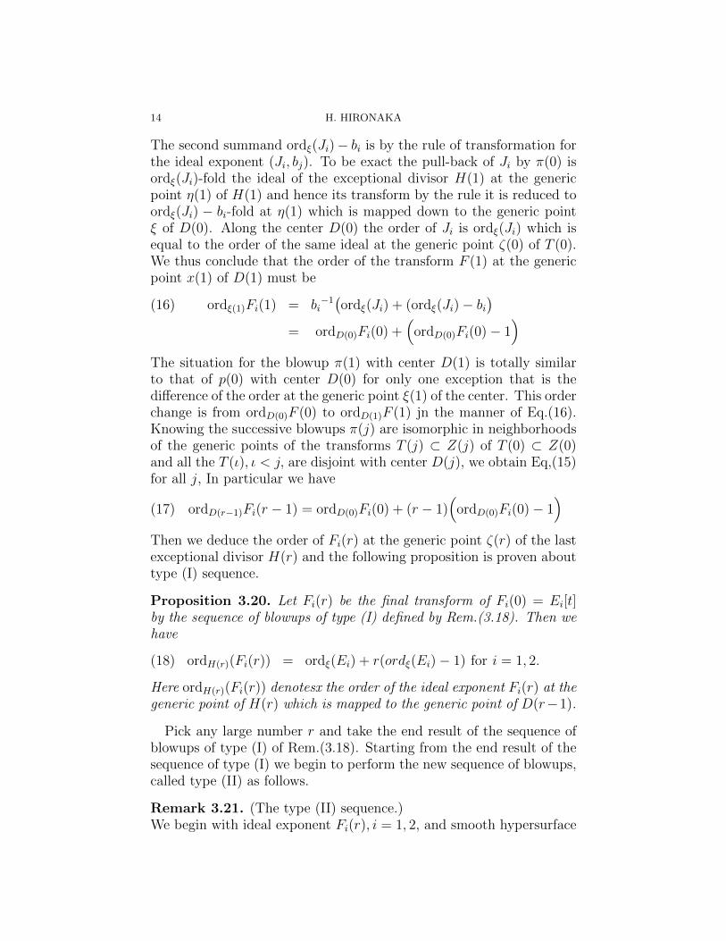
14 H. HIRONAKA

The second summand ordξ(Ji)− bi is by the rule of transformation forthe ideal exponent (Ji, bj). To be exact the pull-back of Ji by π(0) isordξ(Ji)-fold the ideal of the exceptional divisor H(1) at the genericpoint η(1) of H(1) and hence its transform by the rule it is reduced toordξ(Ji) − bi-fold at η(1) which is mapped down to the generic pointξ of D(0). Along the center D(0) the order of Ji is ordξ(Ji) which isequal to the order of the same ideal at the generic point ζ(0) of T (0).We thus conclude that the order of the transform F (1) at the genericpoint x(1) of D(1) must be

ordξ(1)Fi(1) = bi−1(ordξ(Ji) + (ordξ(Ji)− bi

)(16)

= ordD(0)Fi(0) +(

ordD(0)Fi(0)− 1)

The situation for the blowup π(1) with center D(1) is totally similarto that of p(0) with center D(0) for only one exception that is thedifference of the order at the generic point ξ(1) of the center. This orderchange is from ordD(0)F (0) to ordD(1)F (1) jn the manner of Eq.(16).Knowing the successive blowups π(j) are isomorphic in neighborhoodsof the generic points of the transforms T (j) ⊂ Z(j) of T (0) ⊂ Z(0)and all the T (ι), ι < j, are disjoint with center D(j), we obtain Eq,(15)for all j, In particular we have

ordD(r−1)Fi(r − 1) = ordD(0)Fi(0) + (r − 1)(

ordD(0)Fi(0)− 1)

(17)

Then we deduce the order of Fi(r) at the generic point ζ(r) of the lastexceptional divisor H(r) and the following proposition is proven abouttype (I) sequence.

Proposition 3.20. Let Fi(r) be the final transform of Fi(0) = Ei[t]by the sequence of blowups of type (I) defined by Rem.(3.18). Then wehave

ordH(r)(Fi(r)) = ordξ(Ei) + r(ordξ(Ei)− 1) for i = 1, 2.(18)

Here ordH(r)(Fi(r)) denotesx the order of the ideal exponent Fi(r) at thegeneric point of H(r) which is mapped to the generic point of D(r−1).

Pick any large number r and take the end result of the sequence ofblowups of type (I) of Rem.(3.18). Starting from the end result of thesequence of type (I) we begin to perform the new sequence of blowups,called type (II) as follows.

Remark 3.21. (The type (II) sequence.)We begin with ideal exponent Fi(r), i = 1, 2, and smooth hypersurface

SINGULARITIES 15

H(r) in its ambient scheme W (r). Let W (r, 0) = W (r), Fi(r, 0) =Fi(r), i = 1, 2, and H(r, 0) = H(r).

W (r, s)π(r, s− 1)→ W (r, s− 1)⋃

H(r − 1)

π(r, s− 2)→ · · ·

π(r, 0)→ W (r, 0)⋃

H(r, 0)

where all the blowups π(r, j) are isomorphisms because the centersH(r, j) are smooth hypersurfaces, 0 ≤ j ≤ s − 1. The H(r, j) are allisomorphic by themselves. The first center H(r, 0) of blowup of type(II) sequence is the the last exceptional divisor created by the type (I)sequence.

Remark 3.22. Here it is important that the ideal exponents Fi(r, 0) =Fi(r), i = 1, 2, given in the ambient scheme W (r, 0) = W (r) undergonontrivial changes by blowups π(r, k) according to the rule of trans-formation of ideal exponent in spite of no changes for their geometriccarriers by the blowups of type (II) . The rule of transformation dic-tates the ideal exponent Fi(r, k) = (Ji(r, k), bi) in W (r, k) to be trans-formed into Fi(r, k+ 1) = (Ji(r, k+ 1), bi) in W (r, k+ 1) by the rule ofJi(r, k + 1) = h(r, k + 1)−bjJi(r, k)OW (r,k+1)) where h(r, k + 1) denotesthe locally principal ideal defining the exceptional divisor H(r, k+1) inW (r, k + 1). In other words the pull-back of the ideal will loose bi-foldexceptional divisor. Thus we have

(19) ordζ(k+1)(Fi(r, k + 1)) = ordζ(k)(Fi(r, k))− 1

where ζ(j) denotes the generic point of H(r, j), j = k, k + 1..

Remark 3.23. The equality of Eq.(19) is under the condition that theblowup π(r, k) is permissible for Fi(r, k). This condition ls equivalent tosaying that the center H(r, k) ⊂ Sing(Fi(r, k)), i.e, ordζ(k)(Fi(r, k)) ≥ 1because H(r, k) is exactly the closure of its generic point ζ(k). Inview of the equality of Eq.(19) we easily conclude by induction on thenumber e of the type (II) sequence of Rem.(3.21).

(20) ordζ(s)(Fi(r, s)) = ordζ(0)(Fi(r, 0))− s, where Fi(r, 0) = Fi(r)

where the permissibility condition ordζ(s−1)(Fi(r, s−1)) ≥ 1 is assumedfor the blowups π(r, s− 1).

Definition 3.24. After a type(I) sequence of Rem.(3.18) for Fi(0) waschosen, the connecting type(II) sequence of Rem.(3.21) for Fi(r) hasalways the stopping time under the permissibility condition. In otherwords we have the maximum number si(r) such that

ordHi(r,s−1)Fi(r, s− 1) ≥ 1 and ordHi(r,s)Fi(r, s) < 1, for s = si(r).

16 H. HIRONAKA

This number si(r) is the stopping number for Ei for the given numberr � 1. Thanks to Rem.(3.16) we always have si(r) > 0, for i = 1, 2,and in particular s1(r) > 1.

Remark 3.25. In the case of type (I) it should be noted that thepermissibility conditions are valid for all the blowups of the type (I)sequence of Rem.(3.18) thanks to Eq.(17) by which ordD(j)(Fi(j)) ismonotone non-decreasing or increasing with respect j ≥ 0 starting fromordξ(Ei) ≥ 1 for both i = 1, 2 while ordξ(E1) > 1. Remember that the(i)+(II) combined sequence can be an LSB belonging to S(Ei) with anarbitrary r � 1 so long as the number s of R : (II)− 1 is bounded bysi(r).

The following result is the summary of the remarks and propositionsabout the (I) and/(II) type sequences of blowups which are LSB ∈S(Ei) for i = 1, 2, respectively

Proposition 3.26. Under the assumption of Th.(3.15) we have thefollowing consequences.

(1) since S(E1) ⊂ S(E2), we have s1(r) ≤ s2(r) for all choices ofr � 1;

(2) limr 7→∞(s1(r)/r) ≤ limr 7→∞(s2(r)/r);(3) ordξ(Ei) + r

(ordξ(Ei)− 1

)≤ si(r) for i = 1, 2;

(4) si(r) ≤ ordξ(Ei) + r(ordξ(Ei)− 1

)+ 1 for i = 1, 2;

(5) limr 7→∞(si(r)/r) = ordξ(Ei)− 1 for i = 1, 2; and(6) ordξ(E1) ≤ ordξ(E2).

Proof. Item (1) is clear and (2) follows from (1); (3) is already proven byEq.(17); (4) follows from Def.(3.24) together with Eq.(17) and Eq.(18);(5) follows from (3) and (4), dividing the sides of the resulting inequal-ity by r + 1; and (6) follows from (1) and (5). �

Th.(3.15) follows from Prop(3.26).

4. Characteristic algebra ℘(E)

The fundamental tool in our proofs of resolution theorems will bethe characteristic algebra ℘(E) =

⊕d≥0 ℘(E, d). A very important

and useful property of the ℘(E) is that it is not only finitely generated(thus producing useful edge data and edge invariants) but also it has astrong tie with the geometry of infinitely near singularity S(E) of E.To be more explicit we have two different definitions of the same ℘(E),the one geometric and the other algebraic.

SINGULARITIES 17

The geometric definition of ℘(E) is given by letting each ℘(E, a), a >0, be the union of those deals I such that S(I, a) ⊃ S(J, b). It fol-lows that ℘(E) is integrally closed in the graded algebra Bl(Z)∗ =Blposi(Z)

⊕Bl(Z, 0) (defined in Definition 2.2). This is due to the fact

that all the blowups in S have smooth centers and hence the gradedalgebra by the powers of its ideal is integrally closed.

The algebraic definition is as follows: ℘(E) is the integral closure inBl(Z)∗ of the graded O-subalgebra generated by the following idealsof specified homogeneity degrees:

(Diff(j)J)O ⊂ Bl(Z, b− j) for all 0 ≤ j < b

The equivalence of the two definitions has been proven in [23] underthe assumption that the base field K is perfect. The reader should referto the proof of the main theorem of [23], in particular to the Lemmas2.1-2.2 and the claim ([) in page 918 of the [23]. These are containedin the proof of the theorem of the finite presentation of ℘(E) by thetheory of infinitely near singularities in [23]. It should be noted thatthe two definitions are not equivalent in general when the base field Kis not perfect.

Theorem 4.1. The ℘(E) of E = (J, b) is the smallest graded O-subalgebra of Bl(Z)∗ =

⊕a≥0Bl(Z, a) such that

(1) J ⊂ ℘(E, b)

(2) Diff(µ)Z

(℘(E, a)

)⊂ ℘(E, a− µ) for all 0 ≤ µ < a and

(3) ℘(E) is integrally closed in Bl(Z)∗.

In connection with the second property above, we may use Differen-tiation theorem of [24] together with the following lemma.

Lemma 4.2. For a =∑b−1

i=0(b− i)αi with α ∈ Zb0 and for µ < a,

Diff(µ)Z

( b−1∏i=0

(Diff

(i)Z J

)αi) ⊂ ∑β∈Zb0∑b−1

i=0 βi(b−i)=a−µ

( b−1∏i=0

(Diff

(i)Z J

)βi)

Proof. see Remarks (2.1)-(2.2) of the paper [23]. �

Remark 4.3. We add the following supportive comment on the inclu-sion relation of Lem.(4.2) in connection with the second property aboveof Th.(4.1). There the integer µ could be as big as we may want solong as 0 ≤ µ < a with respect to the given a which may be big per se.There the result of differentiation on the left hand side of Lem.(4.2)can have some non-zero factor in summands of the left hand which

18 H. HIRONAKA

may have differentiation of order > b such as i+ µ > b. There we thenreplace the factor by the unit ideal on the right hand side of Lem.(4.2).

With the help of this lemma we can restate the Th.(4.1) as follows.

Theorem 4.4. The ℘(E) is the integral closure of the OZ-subalgebra

OZ[ ⊕

0≤j<b

(Diff(j)Z )J

]⊂ Bl(Z)∗

Theorem 4.5. For every pair of integers a > b ≥ 0 we have the ℘(E, a)viewed as an ideal in OZ is included in the ideal ℘(E, b).

Proof. Let t be an indeterminate over OZ and consider the exten-sion E[t] in Z[t]. Then ℘(E[t], a) = ℘(E, a)OZ[t] which contains theideal t℘(E, a) ⊂ ℘(E, a). Hence by the elementary differentiation∂(a−b) ∈ DiffZ[t]/Z with respect to t we obtain the ideal ℘(E, a) =∂(ta−b℘(E, a)) ⊂ ℘(E[t], a− b) = ℘(E, a− b)OZ[t]. Hence by the ambi-ent reduction modulo tOZ[t] we obtain ℘(E, a) ⊂ ℘(E, a− b). �

4.1. Edge data of ℘(E). Recall blξ(Z) =⊕

d≥0 blξ(Z, d) at each ξ ∈Sing(E)cl. Refer to Definition 2.2 of §2. We have ℘(E, d) ⊂ blξ(Z, d) =max(Oξ)d for every d. Recall ℘(E)ξ =

⊕d≥0 ℘(E, d)ξ of §4.

We define the edge algebra ℘(E)(ξ) of E at ξ as follows.

(21) ℘(E)(ξ) = ℘(E)/(℘(E) ∩max(Oξ)bl(Z)

)where the respective grades and homogeneity of their elements mustbe honored in ℘(E) and in bl(Z). The elements of OZ,ξ as multipliershave all zero degree. Then note the following properties of ℘(E)(ξ).

(1) Pick any regular system of parameters z of Oξ and let z denotethe image of z in bl(Z, 1)/max(Oξ)bl(Z, 1). We then have thesurjection Oξ → K[z] where K[z] is the polynomial ring ofindependent variables z over the residue field K of Oξ.

(2) With respect to the choice of z with z we obtain the inclusions:

℘(E)(ξ) ⊂ K[z] ⊂ bl(Z)ξ/max(Oξ)bl(Z)ξ(22)

and surjection Diff(m)Z,ξ → Diff

(m)K[z]/K ,∀m ≥ 0

which is induced by the surjection OZ,ξ → K[z]. which denotesthe algebra of the differential operators in z over K.

(3) If g = f + h ∈ ℘(E, d) with ordξ(h) > d then f and g have thesame image in ℘(E)(ξ) by the natural epimorphism.

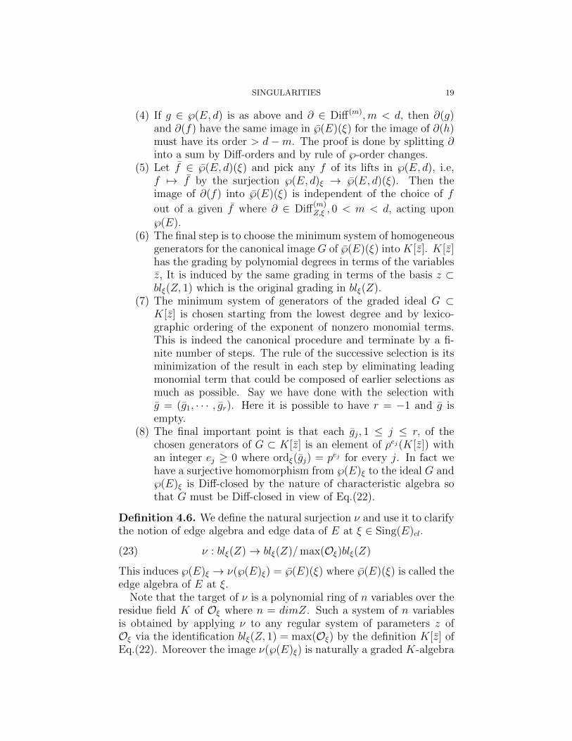
SINGULARITIES 19

(4) If g ∈ ℘(E, d) is as above and ∂ ∈ Diff(m),m < d, then ∂(g)and ∂(f) have the same image in ℘(E)(ξ) for the image of ∂(h)must have its order > d−m. The proof is done by splitting ∂into a sum by Diff-orders and by rule of ℘-order changes.

(5) Let f ∈ ℘(E, d)(ξ) and pick any f of its lifts in ℘(E, d), i.e,f 7→ f by the surjection ℘(E, d)ξ → ℘(E, d)(ξ). Then theimage of ∂(f) into ℘(E)(ξ) is independent of the choice of f

out of a given f where ∂ ∈ Diff(m)Z,ξ , 0 < m < d, acting upon

℘(E).(6) The final step is to choose the minimum system of homogeneous

generators for the canonical image G of ℘(E)(ξ) into K[z]. K[z]has the grading by polynomial degrees in terms of the variablesz, It is induced by the same grading in terms of the basis z ⊂blξ(Z, 1) which is the original grading in blξ(Z).

(7) The minimum system of generators of the graded ideal G ⊂K[z] is chosen starting from the lowest degree and by lexico-graphic ordering of the exponent of nonzero monomial terms.This is indeed the canonical procedure and terminate by a fi-nite number of steps. The rule of the successive selection is itsminimization of the result in each step by eliminating leadingmonomial term that could be composed of earlier selections asmuch as possible. Say we have done with the selection withg = (g1, · · · , gr). Here it is possible to have r = −1 and g isempty.

(8) The final important point is that each gj, 1 ≤ j ≤ r, of thechosen generators of G ⊂ K[z] is an element of ρej(K[z]) withan integer ej ≥ 0 where ordξ(gj) = pej for every j. In fact wehave a surjective homomorphism from ℘(E)ξ to the ideal G and℘(E)ξ is Diff-closed by the nature of characteristic algebra sothat G must be Diff-closed in view of Eq.(22).

Definition 4.6. We define the natural surjection ν and use it to clarifythe notion of edge algebra and edge data of E at ξ ∈ Sing(E)cl.

ν : blξ(Z)→ blξ(Z)/max(Oξ)blξ(Z)(23)

This induces ℘(E)ξ → ν(℘(E)ξ) = ℘(E)(ξ) where ℘(E)(ξ) is called theedge algebra of E at ξ.

Note that the target of ν is a polynomial ring of n variables over theresidue field K of Oξ where n = dimZ. Such a system of n variablesis obtained by applying ν to any regular system of parameters z ofOξ via the identification blξ(Z, 1) = max(Oξ) by the definition K[z] ofEq.(22). Moreover the image ν(℘(E)ξ) is naturally a graded K-algebra

20 H. HIRONAKA

inherited from the grading in ℘(E) ⊂ blξ(Z) but the image is also anideal in the polynomial ring K[z]. We denote ν(℘(E)ξ) by ℘(E)(ξ).

A differential operator ∂ in a graded algebra is said to be homoge-neous if it sends every homogeneous part to some homogeneous part. Inthe cases of our graded algebras, such as Bl(Z), blξ(Z) and ℘(E), everyhomogeneous differential operators has its own degree, say a and sendsall elements of degree k to elements of degree k−a. Our next task is tochoose a minimum system of generators of the ideal ℘(E)(ξ) ⊂ K[z].Keep in mind that K is a perfect field for it is a finite algebraic exten-sion of the perfect field K. It then follows that every element of K isany high power of another member of K.

Remark 4.7. There exists a minimum system of homogeneous gen-erators (g1, · · · , gn) for the edge algebra ν(℘(E)ξ) of the characteristicalgebra ℘(E) of E localized at ξ ∈ Sing(E)cl. The edge algebra is alsoa homogeneous ideal in ν(blξ(Z) which can be identified with the poly-nomial ring of n independent variables over the residue field K of Oξ.These n variables can be obtained as follows.

(1) Choose a regular system of parameters x = (x1, · · · , xn) of Oξ;(2) consider x ⊂ max(Oξ) = blξ(Z, 1) → ν(blξ(Z)) ⊃ x where x is

the image of x by the composition of those maps; and(3) ν(blξ(Z)) = K[x], a polynomial ring of n variables x.

Definition 4.8. Write each element g ∈ ℘(E)(ξ), 6= 0, in the formg =

∑α cαz

α with all cα ∈ K. We then have cβ 6= 0 such that thereis no cα 6= 0 having (|β|, β) ≺ (|α|, α) where | | means the sum ofcomponents and ≺ means that the left side is lexicographically smaller.The monomial term cβ z

β with such β is called the head of g and (|β|, β)is called the signature of g. A system of elements (g1, · · · , gr) is saidto be minimum with respect to z if we have gj ≺ gj+1 for all j.

Definition 4.9. Choose any minimum system of homogeneous gen-erators (g1, · · · , gr) of the ideal ℘(E)(ξ) = ν(℘(E)ξ) in the manner ofRem.(4.7). Then any system of homogenous lift back into ℘(E) of suchgenerators, say (g1, · · · , gr), is called the edge data of E at ξ. Note thatwe then have ordξ(gj) = deg(gj) and

gj = fj + hj fj ∈ ρej(blξ(Z, 1)

)(24)

and

ordξ(hj) > qj = pej = ordξ(gj).

The edge generators of ℘(E)ξ of the form Eq.(24) will be called edgegenerator type. We will then choose the regular system of parameters

SINGULARITIES 21

x of Oξ as follows.

fj = xjqj for all j = 1, · · · , r.(25)

Remark 4.10. Given ξ ∈ Sing(E)cl we let and we can choose a mini-mum system of generators of ℘(E)(ξ) as κ−ξ-algebra which are inducedby a subsystem of generators of the graded algebra℘(E) for a regularsystem of parameters x of Oξ. To be more explicit about role of spe-cial subsystems of x = (y◦(ξ), ω) we have the following technical termswhich will be referred to for later usage. Here we choose {gj, 1 ≤ j ≤ r}of Eq.(24) and x of Eq.(25). However we make renaming as follows:Write gj(ξ) for gj, 1 ≤ j ≤ r, and in particular xk = y◦k(ξ) = gk forthose gk with ordξ(gk) = 1 if any such exist. Indeed it could happen tohave empty set of {gj}, i.e, r = t = 0 if E is not maximum hiked, i.e,

E 6= E in the sense of §6.1.

We define the edge generators and edge parameters as follows.

Definition 4.11. The edge generators are given by

g(ξ) = (y◦(ξ), gt+1(ξ), · · · , gr(ξ)) = (g1(ξ), · · · , gr(ξ))(26)

where, for t = t(ξ) and r = r(ξ), and ordξ(y◦i (ξ)) = 1 for all i,

gk(ξ) = y◦k(ξ), ∀k ≤ t

y◦(ξ) = (y◦1(ξ), · · · , y◦t (ξ))

and

1 < ordξ(g◦t+1(ξ)) ≤ · · · ≤ ordξ(g

◦r(ξ)).

The edge parameters are given by

y(ξ) = (y1(ξ), · · · , yr(ξ)),(27)

which is a part of a regular system of parameters x = (y◦(ξ), ω) of Oξwhere

yi(ξ) = y◦i (ξ) ∈ ℘(E, 1), 1 ≤ i ≤ t

yt+k(ξ) = ωk, 1 ≤ k ≤ r − tgj(ξ) = yj(ξ)

qj(ξ) + εj(ξ) ∈ ℘(E, qj(ξ))

qj(ξ) = pej(ξ), ej(ξ) > 0 t < j ≤ r

ordξ(εj(ξ)) > ordξ(gj(ξ)) = qj(ξ) t < j ≤ r.

The edge exponents are given by

q(ξ) = (1, · · · , 1, qt+1(ξ), · · · , qr(ξ)).(28)

22 H. HIRONAKA

Remark 4.12. When the point ξ is specified we often omit (ξ) fromthose symbols for the sake of notational simplicity. Incidentally thereare included the following special cases: t = 0 and/or r = t. Whenr = t = 0 we say that E is edge-trivial at ξ. Being edge-trivial doesnot mean that ℘(E) is trivial.

Remark 4.13. In positive characteristic cases the study of edge dataof ℘(E) becomes far more important than the case of characteristiczero for the nature of singularity is dramatically different at a non-closed point compared to a closed point. Interesting but sometimeshard questions arise in the cases of points having imperfect residuefields.

4.2. Cotangent module cot(E). Recall

℘(E) =⊕d≥0

℘(E, d)

((2) in §2.7). When we work on the graded algebra ℘(E) for the studyof the singularities of E in terms of local equations we need to choosevarious coordinate systems at each point ξ ∈ Sing(E)cl with respectto the cotangent structure of E at ξ. It is represented by cotangentmodule denoted by cot(E)ξ at ξ.

Definition 4.14. With an integer ` � e where q = pe, e ≥ 0, is themaximum p-power among the edge exponents of Eq.(28) of §4.1 andthe Frobenius p-power is denoted by ρ. We then define the cotangentmodule cot(E, `)ξ and cot(E)ξ as follow.

cot(E)ξ =⋃

all `≥0

cot(E, `)ξ(29)

where

cot(E, `)ξ = p

√ρ`Bl(Z, 1)ξ ∩

(℘(E, p`)ξ + max(Oξ)Bl(Z, p`)ξ

)in which all constituents should honor their homogeneity degrees in℘(E) ⊂ BL(Z) but on occasions of later applications we will needto ignore homogeneity degrees. Since ℘(E) is finitely generated it isclear that some single `� e will define the union of Eq,(29). We thenconsider the constituents and results simply as ideals in OZ .

Definition 4.15. As for the integer ` whose choice is significant inlater applications but it should be noted here that the residue classcot(E)ξ mod max(Oξ)Bl(Z, 1) is independent of ` for all `� q. Thisresidue class, denoted by v(E)ξ, is called the cotangent vector space ofE at ξ, which may be viewed as being dual to the tangent space of E

SINGULARITIES 23

in Z at ξ. A coordinate system x in an open subset V of Z is said tobe allowable for E in V if it contains a system y which induces a basisof c(E)η for every η ∈ Vcl. Symbolically we write xV ⊃ y, or x ⊃ y inshort, for an allowable coordinate system for E in V .

Proposition 4.16. The quantity of Eq.(29) is monotone increasing intrims of ` and hence its local ideal is independent of all `� e.

Proof. Evident by the noetherian property ofOξ. We denote by cot(E)ξfor lim`→∞ cot(E, `)ξ. �

So far has been a strictly local definition of cotangent modules at apoint ξ ∈ Sing(E)cl. However we have a globalized version. Firstly weset a preliminary notion.

Definition 4.17. Let I = I(S) be the ideal of S = Sing(E) ⊂ Z anddefine the global coherent ideal I(m)(S) in OZ such that for every openaffine subset V = Spec(A) ⊂ Z and for f ∈ A we have

(30) ordη(f) ≥ m,∀η ∈ V ∩ Scl ⇔ f ∈ I(m)(S)

This I(m)(S) is uniquely defined as a global coherent ideal in OZ . Wecall it the m-th symbolic power of the ideal of Sing(E).

Definition 4.18. We now define the global coherent cotangent modulecot(E).

cot(E, p`) = p

√ρ`(Bl(Z, 1)) ∩

(℘(E, p`) + I(Sing)Bl(Z, p`)

)(31)

Then cot(E) =⋃`�e cot(E, p`) with q = pe, which is independent of

the choices of `� e and unique for each ξ ∈ Sing(E)cl.

Here the Frobenus ρ maps the quantity under the symbol q√

into

its component-wise p-th power into ℘(E, pq) + I(S)Bl(Z, pq). Hencecot(E, `) is monotone increasing global coherent ideals in OZ .

Hence by the noetherian property we obtain a global coherent ideal

cot(E) =⋃all p`,`�1 cot(E, `)(32)

and hence cot(E, `) = cot(E) for all p`, `� 1.This cot(E) is uniquely defined and called cotangent module of E

which will be effectively used for the study of singularities in particularfor the core-edge focused E of E later discussed later in §6.2.

24 H. HIRONAKA

4.3. Edge Decomposition Theorem.

Theorem 4.19. We obtain the following equivalence which holds withina sufficiently small neighborhood U of ξ ∈ Z.

E ∼( r⋂

i=1

Ei

) ⋂R(E)ξ(33)

or more precisely

S(E) =( r⋂

i=1

S(Ei)) ⋂

S(R(E))

in the sense of the infinitely near singularity S where Ei = (giOU , qi), ∀i,and R(E) = (I, c) with ordξ(I) > c.

(See [22], [23], [24] and [25]). The R(E) is less canonical than the otherEi but there is an explicit way to choose it as follows.

Remark 4.20. Let us define Rξ = ℘(E)ξ ∩ max(Oξ)bl(Z)ξ whichis finitely generated as a graded bl(Z)ξ-module and hence generatedby finitely many ℘(E, j) ∩ max(Oξ)bl(Z)ξ. Hence with the maximumm > 0 of the orders of such a finite system of generators we can choosethe ideal I of R(E)ξ to be ℘(E,m!) ∩ max(Oξ)blξ(Z). It should benoted that Rξ is finitely generated as bl(Z)ξ-module thanks to thefinite generation of ℘(E).

We define the numerical invariants of ℘(E) at ξ as follows.

(34) Invξ(E) = (n, n− r, q1, q2. · · · , qr)with n = dim Z.

4.3.1. Notational warning (1). When we talk about an ideal exponent,such as E = (J, b) as above, we often think of the geometric inter-pretation: the singular locus Sing(E) as a set, or better the set of allinfinitely near singularities S(E), defined in [23].

Readers are cautioned about logical symbols, in particular when ⊂and ∩ are used when dealing with ideal exponents. For instance writing(J1, b1) ⊂ (J2, b2) in short cannot signify anything but S(J1, b1) ⊂S(J2, b2) in the ordinary set-theoretical sense. Also writing (J1, b1) ∩(J2, b2) = (J3, b3) in short cannot mean anything truly but S(J1, b1) ∩S(J2, b2) = S(J3, b3). The intersection is better understood to signify(j1b2 + J2

b1 , b1b2

). We should note that even when b1 = b2 = b the

equality (J1, b) ∩ (J2, b) = (J3, b3) imples

S(J1, b) ∩S(J2, b))

= S(J1 + J2, b)

SINGULARITIES 25

while the converse is not always true. Also J1 ⊂ J2 rigorously impliesthe reversed inclusion S(J1, b) ⊃ S(J2, b) but the converse is not alwaystrue.

It should be kept in mind that geometric implications are often con-venient to deal with, while algebraic ideal-theoretic considerations aremore delicate. This is especially so in the context of the inductionrequired in our proof of resolution of singularities given in this paper.Just for instance the ideal J of E = (J, b) with b > 1 can remain tobe significant by itself even after we gained Sing(E) = ∅ during theprocess of inductive proofs. However it is always true that

(35) S(E1) = S(E2) ⇔ ℘(E1) = ℘(E2)

Refer to [23] and [24]. It will be be seen that our S-geometry is alwaysclosely tied with the ideal exponents up to ℘-equivalence.

Remark 4.21. Unlike ∪ and ⊂ with ideal exponents the rule of trans-forms of ideal exponents by permissible blowups are always explicitand precise as to the pair expression E = (J, b). Refer to Def.(2.1).This fact of matter should be kept in mind. For instance the transformby a permissible blowup can have empty singular locus but the idealof the transformed ideal exponent remains often significant in itself asit is obtained. The significance may become apparent and importantespecially in our inductive proofs of resolution of singularities.

5. The negative degree part of ℘(E).

Recall the graded algebra Bl(Z) of §2.1 of §2 and the characteristicalgebra ℘(E) ⊂ Bl(Z) of Th.(4.1) of §4. Note that Bl(Z) has neg-ative degree part Blnega(Z) unlike ℘(E) = ℘posi(E)

⊕℘(E, 0) where

℘posi(E) =⊕

b>0 ℘(E, b). We write the positive part ℘posi(E, b) of℘(E, b) where 0 < b ∈ Z. We then want to extend ℘(E) by adding℘nega(E) called the negative part of ℘(E, b).

Definition 5.1. Recall BL(Z)◦ =⊕

j≥0BL(Z, j) of Definition 2.2.

We know that the graded OZ-algebra ℘(E) is finitely presented. Thismeans that ℘(E) has a finite system of generators as a BL(Z)◦-module.Fix an integer m > 0 divisible by all the degrees of such a finitelyselected system of generators of ℘(E). For every integer a ∈ Z (positive,zero and negative) we will defineOZ-submodule ℘(E,−a) ⊂ Bl(Z,−a).

℘(E,−a) =∑

d∈Z,dm≥|a|D(m, a, d)(36)

D(m, a, d) = Diff(dm+a)Z ℘posi(E, dm)

When a ≥ 0 we write ℘nega(E,−a) for ℘(E,−a) to emphasize −a ≤ 0.Write ℘nega(E) for

⊕a>0 ℘

nega(E,−a).

26 H. HIRONAKA

In this definition the new notion is only for the case of a ≥ 0. As amatter of fact for a < 0 we have the old parts as follows.

Lemma 5.2. If a < 0 then ℘(E, i) = ℘(E, i) with i = −a

Proof. Pick any d > 0. Then

D(m, a, d) = Diff(dm−i)Z ℘posi(E, dm) ⊂ ℘(E, i)

by the differentiation property inside ℘(E) thanks to Th.(4.2) of §3.Note that for d with md = |a| we have md+ a = 0 so that

D(m, a, d) = OZ,ξ℘(E,−a) = ℘(E, i).

�

Lemma 5.3. Consider the case of a > 0. The sum in the definitionEq.(36) is generated by finitely selected summands. For each integera > 0 the ℘nega(E,−a) is a coherent ρ`(OZ)-module for every suffi-ciently large positive integers `.

Proof. Strait forward by the noetherian O-module of Bl(Z,−a). Thecoherency is thanks to the Noetherean Zariski topology. �

Remark 5.4. It is very important to note that ℘(E, 0) is not alwaysequal to ℘(E, 0) and it could be strictly smaller. The symbol ℘(E, 0)is to show its distinction from ℘(E, 0). We then define ℘(E) to mean⊕

i∈Z ℘(E, i).

Remark 5.5. In view of our main goal of this paper, that is the embed-ded resolution of singularities in p > 0, we often restrict our attentionlocally at a point ξ ∈ Sing(E)cl with the following assumption.

(37) ∃g ∈ ℘(E,m)ξ, ordξ(g) = m > 0

where the m can be replaced by any of its positive multiple togetherwith the corresponding power of g. Therefore we may assume that thesame m can be chosen for both Eq.(37) and Def.(5.1). Incidentary we

will later introduce the notion of maximum base-hiked E of E definedin the section §6. E will have an element g of Eq.(37) locally at every

given point ξ ∈ Sing(E). Incidentally our proof of embedded resolutionof singularities for E will be deduced from the same of all maximumbase-hiked ideal exponents in the same ambient dimension. Refer tothe later comment of Th.(16.4) of §16.1 which will be stated and provenlater.

From now on throughout this section we will be assuming the exis-tence of the element g in Eq.(37) at every ξ ∈ Sing(E)cl. With thisassumption we have

SINGULARITIES 27

Lemma 5.6. The function D(m, a, d) is monotone increasing with re-spect to d for any fixed pair (m, a) with a > 0.

Proof. We prove the statement for the case of a > 0 locally at eachξ ∈ Sing(E)cl. Pick any pair of integers d′ > d and we then have theproof locally as follows.

D(m, a, d′)ξ = Diff(md′+a)℘posi(E,md′)ξ(38)

⊃Diff(md′+a)

(gd′−d℘posi(E,md)ξ

)⊃(

Diff(md′−md)gd′−d)(

Diffmd+a℘posi(E,md)ξ

)= OZ,ξ

(Diffmd+a℘posi(E,md)

)ξ

= D(m, a, d)ξ

where Diff(md′−md)gd′−d = OZ,ξ by the assumption on g. �

Remark 5.7. The D(m, a, d) is monotone increasing with respect tod for a > 0, and fixed (m, a). Hence we can redefine Eq.(36) for a > 0by ∪ instead of

∑as follows.

℘(E,−a) = ℘nega(E,−a) =⋃d:dm>aD(m, a, d)(39)

with D(m, a, d) = Diff(dm+a)Z ℘posi(E, dm)

The D(m, a, d) are all coherent ideals in Bl(Z,−a) ∼ OZ and thenoetherian property of OZ implies that the union Eq.(39) is equal to:

(40) ℘nega(E,−a) = D(m, a, d) = Diff(dm+a)Z ℘posi(E, dm)

for every sufficiently large d with respect to each (a,m). We summarizethe notation for the extended ℘(E) with the tilde-symbols as follows.

℘(E) = ℘posi(E)⊕

℘(E, 0)⊕

℘nega(E)(41)

where

℘nega(E) =⊕a>0

℘nega(E,−a);

℘posi(E) =⊕b>0

℘(E, b); and

℘(E, 0) ∼ OZRecall that ℘(E) = ℘posi(E)

⊕℘(E, 0). We write

℘(E) =⊕i∈Z

℘(E, i).

28 H. HIRONAKA

Note that ℘nega(E,−a), for a > 0, is independent of the choice of mamong those having the property described in Def.(5.1) for D(m, a, d)because we can choose the common multiple for any two different m.Thanks to the monotone increase by this Remark it follows that thedefinition Eq.(36) is not affected at all when we replace m by any ofits positive multiples.

Lemma 5.8. For every pair of integers (i, j) we have

℘(E, i)℘(E, j) ⊂ ℘(E, i+ j)

Proof. Let a = −i and b = −j and the product ℘(E, i)℘(E, j) becomes

D(m, a, d)D(m, b, d)(42)

= Diffdm+a℘posi(E, dm)×Diffdm+b℘posi(E, dm)

⊂

Diff2dm+a+b(℘posi(E, dm)

)2

⊂Diff2dm+a+b

(℘posi(E, 2dm)

)= ℘(E,−a− b)

where 2dm� |a|+ |b|. �

Lemma 5.9. We have the following inclusion relation among ideals:

(1) For integers 0 < a < b the ideal of ℘nega(E,−b) contains theideal of ℘nega(E,−a).

(2) The sum of the two ideals of (1) is contained in the ideal of℘nega(E,−b).

(3) For a < 0 < b the ideal of ℘nega(E,−b) contains the ideal of℘nega(E,−a).

(4) The sum of the two ideals of (1) is contained in the ideal of℘nega(E,−b) contains the ideal of ℘posi(E,−a).

Proof. (1) is proven by Diff(`−a) ⊃ Diff(`−b) for all ` � b and by thedefinition Eq.(39) of Rem.(5.7). (2) follows directly. (3) is proven inthe same way as (1) by means of Diff’s. �

Remark 5.10. It should be noted that, if a+b is negative, the resulting℘(E,−a− b) is nothing but the old ℘(E, a + b) by Lem.(5.2), while ifa + b is positive, then ℘(E,−a − b) is a newly created member of the℘nega(E). In other words, the product operation in the positive part ofthe extended algebra ℘(E) of ℘(E) is identical with the old ℘posi(E).The negative part of ℘(E) is closed by product operation in itself.

SINGULARITIES 29

Theorem 5.11. Assume Eq.(37) at every point of Sing(E)cl. The℘(E) is a OZ-graded algebra whose positive part is identical to ℘posi(E).Moreover its homogeneous parts are all coherent OZ-module.

Proof. By Lem.(5.6), ℘nega(E) is coherent. Lem.(5.2) is about

℘posi(E) ⊂ ℘(E)

and Lem.(5.8) for product inside ℘(E). As for the equality of positiveparts of ℘(E) with ℘(E) is by Lem.(5.2) with Lem.(5.8). �

6. Base-hikes and core-focusing of E

In our inductive strategy for resolution of singularity our initial ques-tion is to ask what would be the best definition of the worst singularpoints of an ideal exponent E. Our ultimate answer will become clearonly after the theory of LLUED (local Leverage-up and Exponent-down) is fully developed in later sections. Here we begin with somepreliminary notions and preparatory work. They are the following twosteps preliminary modifications of the given E = (J, b) with J 6= (0).

6.1. Maximum base-hike E. With E = (J, b), J 6= (0), let d be the

max(ordξ(J)) for ξ ∈ Sing(E)cl and define E = (J, d), called maximum

base-hike of E. The ℘(E) has non-trivial edge data as follows.

Theorem 6.1. For every ξ ∈ Sing(E)cl we have r = r(ξ) > 0 for

E (not necessarily for E) in the expression of edge-data of §26 andedge decompositions by Th.(4.19). Moreover for every d > 0 and every

ξ ∈ Sing(E)cl we have d = ordξ(℘(E, d) provided ℘(E, d) 6= (0).

Proof. Note that E is equivalent to (∏

i ℘(E, i),∑i) where i ranges

through all positive integers i ≤ b such that ℘(E, i) 6= (0). With the

maximum ordξ(J) = d > 0 in E = (J, d) we have a nonzero element in℘(J, d) mod max(Oξ)Blξ(Z),∀ξ. Its differentiations produce nontriv-ial edge generators and edge data at ξ. �

Remark 6.2. Later in §(16.1)) we prove Th.(16.4), renamed Theorem∆, which states that if we have the resolution for every maximumbase-hiked ideal exponent in every ambient scheme having the samedimension as n = dimZ, then we have the resolution of E itself. Atthis point we continue to develop the main concepts and key techniquesneeded to prove our main result: resolution of singularities in p > 0.Theorem ∆ of §(16.1) is a kind of prelude to the main theorems ∇ I-II-III of §(16.2) and §(16.3). Some readers may wish to skip forward toTh.(16.4) and its proof in §(16.1) because it is independent and simpler

30 H. HIRONAKA

to state in comparison with §(16.2) and §(16.3) which will commandmuch heavier preparation.

6.2. Core focusing E. Let Invmax(E) denote the lexicographical max-

imum of Invξ(E) for all ξ ∈ Sing(E)cl. We then have an ideal exponent

E naturally associated with E such that

℘(E) ⊃ ℘(E) and(43)

Sing(E)cl = {ξ ∈ Sing(E)cl | Invξ(E) = Invmax(E)}

where ℘(E) is the maximum under these conditions. We can define thesame E as follows. With the maximum invariant

Invmax(E) = (n, n− r, q1 · · · , qr)we pick any E such that

(44) S(E) = ∩1≤i≤r S((℘(E, qi), qi

))∩ S(E)

holds. The E will be called the core-edge focusing of E (also that ofE). We write and use the following symbol.

(45) E 99K E 99K E

for the composed process of core-edge focusing after maximum base-hike. From now on we will only be working with E until we come tothe last section of Part 1 in which we begin making use of blowups forthe first time in order to prove Main Theorems I,II,III.

6.2.1. Relation between ℘nega and ℘posi.

Theorem 6.3. Assume that we have an element g ∈ ℘(E, q)ξ ofEq.(37) at a point ξ ∈ Sing(E)cl. We then assert that an elementf with 0 6= f ∈ Oξ belongs to ℘nega(E,−a)ξ with a ∈ Z if and only if

(46) gp`

f ∈ ℘(E, qp` − a) for all `� 1.

Here the a could be either positive, zero or negative. Moreover if h ∈℘nega(E,−a)alg then hf ∈ ℘(E, d− a) for all h ∈ ℘(E, d), d ≥ a

Proof. The only-if-part of the claim is immediate from the algebraicproperty (in particular the graded product rule) of E. In order to provethe if-part that is to prove f ∈ ℘(E,−a) for the given f ∈ Bl(Z,−a)it is better to generalise the question a little as follows. Namely pickany h ∈ ℘(E, d), d ≥ 0, we assume the Eq.46 applied hf ∈ Bl(Z, d−a)instead of f and prove hf ∈ ℘(E, d−a) including the case in particularwe have d − a ≥ 0. This way we can assume that the addition off ∈ ℘(E,−a)alg, a > 0, to E does not affect maintaining ℘posi(E) as

SINGULARITIES 31

it is. Now we assume gp`hf ∈ ℘(E, qp` + d − a),∀` � 1, and we

want to prove fh ∈ ℘(E, d − a). We pick and fix a regular system ofparameters x of Oξ and recall the notations of elementary differentialoperators with respect to x in the sense of Def.(3) with Eq.(8). Pickany ξ ∈ Sing(E)cl where we work locally. Let K[[x]] be the localcompletion of Oξ with a regular system of parameters. Let ∂α be anelementary differential operator such that |α| = q and ∂αg is a unit

u ∈ Oξ. Consider the elementary differential operator ∂(`) = ∂p`α.

We then have ∂(`)(ρ`(X)) = ρ`(∂αX) for every X ∈ O. Consider anelementally differential operator ∂α such that |α| = q and ∂αg is a unitin K[[x]]. For sufficiently large `� ordξ(fh) we have

(47) ∂(p`α)(gp

`

fh)≡ up

`

fh mod max(Oξ)p`

In fact we have, for (∂(α))p`(g) = up

`fh,

∂(p`α)(gp`

fh) =∑

β∈Zn0 :α∈β+Zn0

(α

β

)(∂(β)g)p

`

∂(p`(α−β))(fh),

which is contained in max(O)p`. We therefore have

∂(p`α)(gp`fh) = up

`fh+B with B ∈ max(O)p

`

Eq.(47) is now proven. On the other hand we have gp`fh = (gp

`f)h ∈

℘(E, qpp` − a + d) by the assumption on (g, f) and by h ∈ ℘(E, d).

Hence ∂(p`α)(gp`fh) ∈ ℘(E,−a + d) Knowing that u is a unit we thus

conclude that for all `� 1 we have

(48) gh ∈ ℘(E,−a+ d) + max(O)p`

Now by taking the limit ` → ∞ we obtain fh ∈ ℘(d − a)K[[s]] withthe local completion K[[s]] of Oξ. Since K[[s]] is faithfully flat over Oξwe conclude fh ∈ ℘(d− a)ξ. �

Theorem 6.4. Assume that E = E, i.e, E is maximum base-hiked inthe sense of §(6.1). We claim that the extended ℘(E) is differentiation-closed, or diff-closed for short, in the sense that for every degree d,either positive or negative, we have ∂(℘(E, d)) ⊂ ℘(E, d− µ) for every

∂ ∈ Diff(µ)Z with µ ≥ 0.

Proof. By Th.(6.1) of §(6.1) we have some g at any given point ξ ∈Sing(E)cl. Now if f ∈ ℘(E,−a)ξ, a > 0, then gp

`f ∈ ℘(E, qp` − a)ξ

for all ` � 1. Then for any given ∂ ∈ Diff(µ)Z and for any p` � qµ

we have ∂(gp`f) = gp

`∂(f) belongs ℘(E, qp` − a − µ)ξ. We then have

32 H. HIRONAKA

∂(f) ∈ ℘(E,−a−µ)ξ thanks to Th.(6.3). This works for any a, positiveor negative. Refer to the three key theorems of [24]. �

Theorem 6.5. Let g be an element of ℘(E, q)V with ordξ(g) = q ≥a > 0 where V 3 ξ is an open neighborhood to which g extends with thesame property. We then assert that

℘nega(E,−a) ⊂(49)

Ker(σ : OV → ℘(E, q)/(℘(E, q − a) ∩ ℘(E, q)

)where σ is the OV -homomorphism which maps every f ∈ OV to theclass of gf in the target quotient module.

Proof. In fact we have that if f ∈ Ker then gf ∈ ℘(E, q−a)V ∩℘(E, q)Vwhich is equivalent to gf ∈ ℘(E, q − a)V . Hence gp

`f = gp

`−1gf ∈℘(E, q(p` − 1) + q − a) for all `� a. We obtain f ∈ ℘(E,−a). �

Theorem 6.6. Assume that E = E in the sense of §6.2. Then℘nega(E,−a) is coherent O-module for all integers a > 0.

Proof. Immediate by Th.(6.5). �

Theorem 6.7. Consider a pair of ideal exponents E and F such that℘(E) ⊃ ℘(F ) so that ℘(E) ⊃ ℘(F ). Assume that there exists someg ∈ ℘(F, q)ξ of Eq.(37) at every point ξ ∈ Sing(F )cl, We then have

℘nega(E) ⊃ ℘nega(F ). For instance if F = F then the same is true.

Proof. The proof is straight-forward by the definition of ℘nega in Eq.(36)of Def.(5.1). �

Definition 6.8. Notation x ⊃ y will be called an allowable coordinatesystem for E at a point ξ ∈ Sing(E)cl if x is a regular system of param-eters of OZ,ξ such that y is member of x (usually the first component)and is also a generator of cot(E)ξ.

Remark 6.9. The LL-head module is generated by cotangent param-eters y extendable to a regular system of parameters x ⊃ y of Oξ. TheLL-head module a L(E) is marked with an integer ` > 0 called itsdepth.

Definition 6.10. Firstly we define the coherent ideal L(E)

(50) L(E) =∑j>0

{f ∈ ℘(E, j) : Diff(j)Z f ⊂ ℘(E, j)}

and the cotangent algebra of ℘(E)

(51) cot℘(E) = ℘(E)/L(E).

SINGULARITIES 33

It should be noted that the fibre of cot℘(E) at each ξ ∈ Sing(E)cl isthe polynomial algebra κ(ξ)[g(ξ)i, 1 ≤ i ≤ r(ξ)] where g(ξ) denotes thesystem of the residue classes of the edge generators of ℘(E)ξ. Refer tothe module of LL-heads L(E) below.

6.3. Coherent LL-heads module L(E). Recall Eq.(31) of Def.(4.18)after Eq.(29) of §4.2 about cot(E, q) and cot(E).

Theorem 6.11. Pick any element g = yq + ε ∈ ℘(E, q)ξ with q =pe, e > 0, where ξ ∈ Sing(E)cl. Assume that ordξ(y) = 1 and ordξ(ε) >q. Then y ∈ cot(E). Conversely every element y ∈ cot(E) withordξ(y) = 1 we find g and ε satisfying the assumption of Th.(6.11).

Proof. By the equation Eq.(29) the assumption implies y ∈ cot(E).The converse is also true because of the same equation. �

Definition 6.12. Let V be an open subset of Z and consider integers`� 1. Then an LL-head of order q of E along Sing(E) ∩ V means anelement g ∈ ℘(E, q)(V ) having the following property.

g = yq + ε ∈ ℘(E, q)(V ) for q = pe, e > 0,(52)

ordη(y) = 1 and ordη(ε) > q for all η ∈ Sing(E) ∩ Vcl.

We choose ` � q so that the set of all LL-heads g as above form anρ`(O)V -module.

We let L(E, q, `)V denote the ρ`(O)V -module generated by all LL-heads of order q of E along Sing(E)V . The ` is called the depth ofL(E, q, `)V . It should be noted that with every sufficiently large integer` we have a global coherent ρ`(O)-module

(53) L(E, `) =⊕

q(j)=pj ,j∈Z0

L(E, q, `)

Locally a typical example of g ∈ L(E)ξ is any of the edge generatorsof ℘(E) at ξ. Refer to §4.1. We write q for the maximum qr(ξ) amongthe powers of p in the Eq.(28) of §4.1. Then the numbers ` of Def.(6.12)must have ` > q at least and often bigger as we see later with referenceto the notion of LL-chains in §9.8 later. Another notion (weaker ingeneral) called LL-prehead is introduced in Eq.(54) below. Note thatthe core-edge focusing is essential for the LL-heads to be non-trivial.

L(E, q)ξ = ℘(E, q) ∩ max(Oξ)blξ(Z) =(54)

{f ∈ ℘(E, q)ξ |Diff(k)Z f ⊂ blξ(Z, q − k + 1),∀k < q}

34 H. HIRONAKA

We write L(E)ξ =⊕

j>0 L(E, q(j)) with q(j) = pj and L(E, q(j)) is

a ρ`(O)-module for every ` > j. Its member is called LL-prehead ofdegree q(j) of E.

Remark 6.13. Note that we have

L(E, q(j)) ⊂ L(E, q(j)) for ∀j(55)

g ∈ L(E, q(j))⇔ g ∈ L(E, q(j)) and ordξ(g) = q(j)

and

g ∈ L(E, q(j)) and f ∈ L(E, q(j)) \ L(E, q(j))⇒ g + f ∈ L(E, q(j)).

Theorem 6.14. For every point ξ ∈ Sing(E) and for every positiveinteger `(0) > 0 there exists an open affine neighborhood V of ξ ∈ Zsuch that for every ` ≥ `(0)

(1) we have a finite system g∗ = (g1, · · · , gr) with gi ∈ O(V ) for alli and g∗ is a system of edge generators of ℘(E) at every pointη ∈ Vcl∩Sing(E) in the sense of Eq.(26). (For this we need theassumption that E is core-edge focused.)

(2) We have a finite system of homogeneous elements generating

I(Sing(E))Bl(Z) ∩ ℘posi(E) that is(56)

∩η∈Sing(E)clmax(Oη)blη(Z)℘(E)

which is an ideal in the noetherian graded algebra ℘(E).

where I(Sing(E)) denotes the ideal of Sing(E) ⊂ Z). It shouldbe noted that Sing(E) is viewed as a reduced subscheme of Zand I(Sing(E)) is a radical ideal.

(3) The Eq.(56) is an ideal in the noetherian graded ρ`(O(V ))-algebra and hence it is generated by finitely many homogeneouselements {fj} as ρ`(blζ(V ))-module.

(4) The finite generation of I(Sing(E))Bl(Z) ∩ ℘posi(E) as aboveshould be understood as ρ`(Bl(Z))-module with every ` ≥ `(0).

Thus for every ζ ∈ Vcl ∩ Sing(E) and for every g ∈ L(E)ζ we writeg = g′ +

∑j Bjfj with g′ ∈ ρ`(O)(V )[g∗] and Bj ∈ ρ`(blζ(V )).

Proof. Follows immediately from Eq.(52), Eq.(54) and Eq.(55) �

Definition 6.15. A paired system (g∗; f) of Th.(6.14) is called a setof edge-inner generators of L(E)V in an open affine V and with depth`.

SINGULARITIES 35

7. Permissible transformations and effects on ℘(E)

Given E = (J, b) furnished with ℘(E) and S(E) in the ambientscheme Z we pick a point ξ ∈ Sing(E)cl and choose an edge decompo-sition of E locally at ξ by Th.(4.19). We then define and examine thetransforms of the edge data of ℘(E) by permissible blowups for E andelucidate the changes in the edge invariants Invξ(E) of Eq.(34).

7.1. Effects on edge data of ℘(E). Consider a blowup π : Z ′ −→ Zwith center D 3 ξ permissible for E. Write I = I(D,Z), the idealof D ⊂ Z. Note that π is then automatically permissible for everyEi = (giRξ, qi), 1 ≤ i ≤ r, of the local edge decomposition of Th.(4.19).

Theorem 7.1. We assert that the edge invariants never increase inthe sense of lexcographical ordering. To be precise we pick any pointξ′ ∈ π−1(ξ) ∩ Sing(E ′)cl with the transform E ′ of E by π so thatξ′ ∈ π−1(ξ) ∩

(∩1≤i≤rSing(E ′i)

). We then have Invξ′(E

′) ≤lex Invξ(E).(Refer Eq.(34).)

Theorem 7.2. Let I = I(D,Z), the ideal of D in OZ. Pick any ξ′ ofTh.(7.1) and any exceptional parameter z for π at ξ′, i.e, z ∈ I(D,Z)ξand zOZ′,ξ′ = I(π−1(D), Z ′)ξ′. We then assert:

(1) There exists ci ∈ OZ,ξ such that yi = yi − ci ∈ Iξ and y′i =z−1yi ∈Mξ′ for all i. Moreover (y′, z) is extendable to a regularsystem of parameters of OZ′,ξ′ where y′ = (y′1, · · · , y′r).

(2) If Invξ′(E′) = Invξ(E) we then have ordξ′(g

′i) = qi with g′i =

z−qigi for all i and moreover(3) the pair (g′, y′) with g′ = (g′1, · · · , g′r) is an edge data yielding

an edge decomposition of E ′ locally at ξ′ as follows.

(57) S(E ′) =( r⋂

i=1

S(E ′i)) ⋂

S(F ′)

where E ′i = (g′iOZ′,ξ′ , qi), 1 ≤ i ≤ r, and F ′ is the transform ofF by π at ξ′. Refer to Th.(4.19) of (4.3).

The lemmas below are stated and proven in such a manner thatproofs of the theorems above are all therein included. For notationalsimplicity we write Rξ or R for OZ,ξ and Mξ or M for max(OZ,ξ).

Lemma 7.3. The permissibility of π implies that the ideal I of thecenter contains yi − ci, denoted by yi, with ci ∈M2

ξ for every i.

Proof. The permissibility implies gi = y qii −εi ∈ Iξqi and with ordξ(εi) >qi. Hence εi mod Iξ is a qi-th power in R = Rξ/Iξ. It is also in

36 H. HIRONAKA

max(R)qi+1 because εi ∈ Mξqi+1. Therefore εi mod Iξ must be in

max(R)2qi from which there follows the existence of ci. �

Lemma 7.4. (y1, · · · , yr, z) extends to a basis of the ideal I as well asto a regular system of parameters of Rξ. We can choose those ci ofLem.(7.3) so that z−1yi ∈ Mξ′ = max(OZ′,ξ′) for all i. For instance ifκξ = κξ′ we can choose ai ∈ Rξ which is congruent to z−1yi moduloMξ′ and then replace ci by ci + aiz. By choosing this instead of ci ofLem.(7.3) we gain the claimed property of z−1yi, 1 ≤ i ≤ r.

Proof. The first claim is immediate from Lem.(7.3). Let us write gi =y qii + ε∗i . Then we must have ε∗i in I qi

ξ ∩Mqi+1ξ = Mξ I

qiξ . Now pick an

exceptional z ∈ Iξ for π at ξ′. Then z−qiε∗i ∈ Mξ′ and hence z−qiy qii ∈Mξ′ by the assumption ξ′ ∈ Sing(E ′i)cl. We conclude z−1yi ∈ Mξ′ forall i. This proves Lem.(7.4) as well as the following Lem.(7.5). �

Lemma 7.5. After replacing y by Lem.(7.4) we obtain the new edgeparameters y′ = (z−1y1, · · · , z−1yr, z) extendable to a regular system ofparameters of Rξ′ = OZ′,ξ′.

Lemma 7.6. If Invξ′(E′) ≥lex Invξ(E) then Invξ′(E

′) = Invξ(E) andthe transform E ′i is (g′iOZ′,ξ′ , qi) with g′i = z−qigi for every i. Also thetransform E ′ of E by π has an edge decomposition as follows.

(58) S(E ′) =( r⋂

i=1

S(E ′i)) ⋂

S(F ′)

within a neighborhood of ξ′ in Z ′. cf.(4.3)

Proof. The assumption ξ′ ∈ Sing(E ′)cl implies ξ′ ∈ Sing(E ′i)cl andhence ordξ′(g

′i) = ordξ(gi) for every i. Hence the assumption on the

edge invariants at ξ′ implies that g′i, 1 ≤ i ≤ r, are enough to generatethe edge data of ℘(E ′) at ξ′. Thus Eq.(57) and the Inv equality. �

7.2. The rule of transformation of ℘nega.

Remark 7.7. The rule of transformation for ℘naga(E) is deduced bythe known rule for ℘posi(E) thanks to the product rule of Lem.(5.8)for ℘(E). Geometrically speaking the transform of ℘nega(E,−a) isadding a-times exceptional divisor while the transform of ℘nega(E,+a)is deleting a-times exceptional divisor after taking the pull-back byblowup. To be precise algebraically we have the following theorem.

In the following theorem we are assuming Eq.(37) at every point in

Sing(E)cl. Indeed this condition is always true if E = E and/or E = E.As for the effect of permissible transformation upon the Inv-invaiants

SINGULARITIES 37

we have a good reference with Lem.(7.3), Lem.(7.4), Lem.(7.5), Lem.(7.6)following after Th.(7.1).

Theorem 7.8. For every finite sequence of local blowups π : Z ′ → Zwith centers Di, 0 ≤ i ≤ r, permissible for the successive transformsEi ∈ Zi from E = E0 ∈ Z = Z0 up to E ′ = Er ∈ Z ′ = Zr in the sense ofDef.(2.4). We then claim that for every point ξ′ ∈ π−1(ξ)∩ Sing(E ′cl)clwith Invξ′(E

′) = Invξ(E) in the sense of Eq.(34) we have

(59) ℘nega(E ′,−a)ξ′ =(∏

i

I(Di, Zi)a)(℘nega(E,−a)OZ′

)ξ′

where I(Di, Zi) is the ideal of Di in OZi. The integer a may be any butthe important cases are for a > 0. The cases for i = −a > 0 are directfrom the definition of ℘posi(E).

Proof. A proof of Eq.(59) can be done by strait application of prod-uct rule Lem.(5.8) and by the known rule of transformation for eachhomogeneous parts of ℘posi(E). �

Remark 7.9. Here is a more direct argument. We have ℘nega(E,−a) =

Diff(md+a)℘(E,md) for d � a in the manner of Def.(5.1) supportedby Lem.(5.6) and Lem.(5.8). We also have (ρ`(g))(℘nega(E,−a)) ⊂℘posi(E,mp` − a). The I(D,Z)OZ′ = I(D′) is the the ideal of theexceptional divisor D′ = π−1(D) in Z ′. This ideal is locally principal.Choose a generator z of the localized I(D′)Oξ′ Now by the permissibleπ we have the blown-up results at ξ′ in all details as follows.

℘nega(E,−a)Oξ′ (pulback by π)(60)

= g−p`

℘posi(E,mp` − a)Oξ′ (degree up by multiplier)

= z−mp`

zmp`−a℘posi(E ′,mp` − a)Oξ′ (rule for ’posi’ case)

= z−a℘posi(E ′,mp` − a)Oξ′= z−a(g′)p

`

℘nega(E ′,−a)ξ′ (degree down by division)

= z−a℘nega(E ′,−a)ξ′ (unicity of g′ = z−mg at ξ′)

= I(D,Z)−a(℘nega(E ′,−a)

)ξ′

With this for all ξ′ there follows Eq.(59).

We have the following technical but very useful lemma.

Lemma 7.10. Let h ∈ BLξ(Z,−k) with k ∈ Z and assume that wehave the inclusion of Eq.(62) for all ` � 1. Then we claim h ∈℘(E,−k). Note that in this lemma the number k can be positive, neg-ative or zero.

38 H. HIRONAKA

Proof. Pick and fix a regular system of parameter x of OZ,ξ. We then

have a differential operator ∂ ∈ Diff(m) such that ∂(h) = 1. In factby the condition on g of Eq.(37) we can find an elementary differentialoperator δ in x of degree m such that u = δg is a unit. Then let∂ = u−1δ. Then let σ be the differential operator in ρ`(Oξ) which is

σ = ρ`∂ρ−`. Then let ∆(`) ∈ Diff(mp`) be the x-Cartier extension of σin the sense of Def.(3.7) supported by Lem.(3.6). Now let K[[x]] denote

the local completion Oξ where K is the algebraic closure of K insidethe completion. Let us write

h =∑

β cβxβ and h(`) =

∑β:βi<`,∀i cβx

β(61)

where cβ ∈ K, ∀β ∈ Z0n

Recall that every differential operator in Oξ has its unique exten-sion to such in K[[x]]. By the x-Cartier property we have ∆(h) ∈ρ`(max(K[[x]]). Remember that ∆(ρ`(g)) = 1 while ∆(xβ) = 0 everyβ with 0 ≤ βj < p`,∀j. Therefore ∆(g`xβ) = xβ and h − ∆(g`h) ∈(x)`K[[x]] for every ` � 1 where ∆(g`h) ∈ ℘nega(E,−k). Hence h ∈℘nega(E,−k)+(x)`K[[x]],∀`� 1 whch implies h ∈ ℘nega(E,−k)K[[x]].This implies h ∈ ℘nega(E,−k) because K[[x]] is faithfully flat over thelocal ring O. �

Theorem 7.11. Under the assumption of Th.(7.8) we have the follow-ing facts.

(1) ℘(E) is diff-closed in the sense that for every integer j ∈ Z, 6= 0,

we have Diff(c)Z ℘(E, j) ⊂ ℘(E, j − c) for every integer c > 0

(2) ℘(E) is integrally closed in the graded algebra Bl(Z)

Proof. As for (1) if j > 0 then ℘(E, j) = ℘posi(E, j) and hence the in-clusion is either by the property of ℘(E) with c ≤ j or by the definitionEq.(36) of ℘(E, j − c) with c > j. If j < 0 let a = −j and ℘(E, j) =

Diff(md+a)℘posi(E,md) with d � 1 by Eq.(40). Hence Diff(c)℘(E, j)

is Diff(c)Diff(md)+a℘posi(E,md) which is contained in ℘(E,−a − c) bydefinition. Here −a − c = j − c. As for (2) it is enough to exam-ine the case of negative integration thanks to Th.(5.11). Pick anyh ∈ BLξ(Z,−k), k > 0, which is integral over ℘(E). In view of themutual independence of homogeneous parts we must have an equa-tion hα+

∑0<β≤α fβh

α−β = 0 with fβ ∈ ℘nega(E, β). Then by choosing

`� 1 we examine the multiplication of the equation above by (ρ`(g))α.Namely

(ρ`(g))h)α +∑

0<β≤α

(ρ`(g))βfβ)(ρ`(g))h)α−β = 0

SINGULARITIES 39

with g and m of the assumption Eq.(37). Note that we then have(ρ`(g))βfβ ∈ ℘posi(E,mp`β) for all β so that (ρ`(g))h is integral overwpposi(E) and hence

(62) (ρ`(g))h ∈ ℘posi(E,mp` − k) with g of Eq.(37)

thanks to the integral closed ℘(E). Note that Eq.(62) is valid forevery choice of ` � 1. Now thanks to Lem.(7.10) we conclude h ∈℘nega(E,−k). Th.(7.11) is thus proven. �

7.3. Rule of transformation for ℘nega. On the rule of permissibletransformation on ℘nega(E) here is an important addition to Th.(7.8)again due to Eq.(83) and Eq.(84).

Theorem 7.12. Let π : Z ′ → Z with center D be permissible for Eand let E ′ be the transform of E by π. Pick a point ξ′ ∈ Sing(E ′)cl withξ = π(ξ′) ∈ Sing(E). Assume that we have a nonzero edge generatorg′ of E ′ at ξ′ which is the transform of an edge generator g of E atξ. Then locally at ξ′ we have that ℘nega(E ′) contains the transform℘nega(E)′ of ℘nega(E) by π.

Proof. The proof is straight forward by Th.(6.3). In fact for every

element f ∈ ℘(E,−a) with a > 0 we have gp`f ∈ ℘(E, qp` − a). Then

g′p`

f ′ ∈ ℘(E ′, qp` − a) with the transform f ′ of f by π. �

7.4. Coordinate translation in p > 0.

Definition 7.13. Let V be an open set in Z and let x = (x1, · · · , xn)be a system of elements in O(V ). We call x a coordinate system of V iffor even point ξ ∈ Vcl∩Sing(E) we find a regular system of parametersz = (z1, · · · zn) such that the differentiation matrix of x with respect toz is invertible in the local ring Oξ.

We consider a regular system of parameters x = (y, ω) at ξ ∈Sing(E)cl which is naturally extended to regular parameters on a suf-ficiently small affine neighborhood V 3 ξ in Z. For each point η ∈V ∩ Sing(E)cl we then have the local completion Oη = K(η)[[x − a]]with a ∈ K(η)n where K(η) is the algebraic closure of the base field

K inside Oη. This fact is due to the assumption that K is a perfectfield and κη is separable algebraic over K. It should be noted herethat (x − a) is a regular system of parameters in K(η)[[x − a]] butnot necessarily in Oη. However all elementary differential operatorsin x make sense as differential operators in K(η)[[x − a]] which coin-cide with the elementally differential operators with respect to x−a inK(η)[[x− a]]. Now we want to obtain a regular system of parameters

40 H. HIRONAKA

of Oη which are approximations of x−a well suited to our work relatedto LLED-operations of later sections such as §9.

Lemma 7.14. Given η ∈ Vcl and a unit f ∈ Oη we have fN ∈ Oη forevery integer N � 1 such that f ≡ ρN(fN) mod max(Oη). It followsthat in a situation of the formal translation x− a with a ∈ Kn we canfind aN ∈ Oηn such that a− ρN(aN) ∈ max(K[[x− a]])n. We will usex−ρN(aN) in Oηn as a useful approximation of x−a in later sections.

Proof. Given f we let κ ∈ K be the residue of f at η. Then Fork = pN

√κ ∈ K and pick fN ∈ Oη whose residue class at η is k. �

Corollary 7.15. Under the assumption of Lem.(7.14) and given anyfinite number of differential operators ∂j, 1 ≤ j ≤ s in DiffV we haveN � 1 such that for every monomial xα we have ∂j

((x− ρN(aN))α

)=

∂j(xα) for every j.

The proof of this corollary is immediate from Lem.(7.14). It shouldbe noted that x− ρN(aN) with N � 1 is a good rational substitute forthe formal translation x− a with a in the algebraic closure of the basefield K. It is useful in many of the consequent sections. In particularrefer to those differentiations later in §9.5 which will be indispensablefor the proofs of the LLUED theorems stated in Th.(9.2) and (9.3).

Definition 7.16. We call x − ρN(aN) a regular translation of x withdepth N at η.

Theorem 7.17. For any coherent ρ`(O)-submodule W of ℘nega(E,−a)with ` � a and for a point ξ ∈ Sing(E)cl, if W (ξ) = (0) then thereexists an open affine neighborhood V of ξ ∈ Z such that W (η) = (0)for every η ∈ Sing(E) ∩ Vcl.Proof. Note that we have a finite number of differentiations {∂f} whichlocally generate ℘nega(E,−a)ξ as ρ`(O)-module within a small enoughaffine open neighborhood V of ξinZ. Then for each η ∈ Sing(E) ∩ Vclwe apply the translation from ξ to η such as x − ρN(aN) for a chosencoordinate system x in V in the manner of Lem.(7.14). �

7.5. Cleaning by edge equation g = yq + ε. The self-cleaning of gor g-cleaning of ε is defined first formally in the local completion Oξand then by its approximation in O modulo ρN(O) with a sufficientlylarge integer N � (1 + e)n with q = pe and n = dimZ.

Choose a regular system of parameters x = (y, ω) of Oξ. It is impor-tant that x contains y of the given LL-head g = yq + ε. Let us writethe local completion Oξ = K[[y, ω]] of the unique algebraic extensionK of the base field K.

SINGULARITIES 41

Then we have Oξ =∑

0≤j<q yjK[[g, ω]] thanks to the assumption

that ordξ(ε) > q by the definition of Lξ. Hence we can write

(63) ε =∑k≥0

gk( ∑

0≤j<q

yjσ(k, j))

with σ(k, j) ∈ K[[ω]],∀(k, j).

Definition 7.18. Define the formal g-cleaning of ε to be

(64) ε](∞) =∑

0≤j<q

yjσ(0, j),

not necessarily any element of Oξ. We rather look for its approxi-mations by elements of Oξ which help to prove global resolution ofsingularities (not merely the local or formal uniformizations). We thuspick an integer N � (1 + e)n. We note that

ε− ε](∞) =∑

k≥1,0≤j<q

gkyjσ(k, j) = gA(N) + gB(N)(65)

where

A(N) =∑

k≥1,0≤j<q

yj∑

kq+|β|≤pNgk−1ωβτ(k, j, β)

σ(k, j) =∑τ

ωττ(k, j, β) with τ(k, j, β) ∈ K, ∀(k, j, β)

B(N) =∑

k≥1,0≤j<q

gkyj∑

kq+|β|>pNgk−1ωβτ(k, j, β).

Note that B(N) ∈ ρ`(max(K[[x]]). Then for each τ ∈ K we pickf ∈ Oξ which is ≡ Q

√τ mod max(Oξ), and define τN = ρN(f) ∈ Oξ.

We then define an approximation AN of A as follows:

AN =∑

k≥1,0≤j<q yj∑

kq+|β|≤pN gk−1ωβ

(τ(k, j, β)N

)(66)

and A− AN ∈ ρN(max(K[[x]]))

We now define

(67) ε](N) = ε − gAN

which will be called a (rational) g-cleaning of ε to the depth N .

We have

ε ≡ ε](N) modulo∑k>N−e g

kK[[x]] +∑

j≤q yj∑

kq+|β|≤pN gk−1ωβ max(ρN(K[[x]]).

Lemma 7.19. We have

ε](∞) ≡ ε](N)

42 H. HIRONAKA

where the equivalence is modulo

gρN−e(max(K[[x]])) + gOξ max(ρN(K[[y, ε]]).

Proof. This is proved by direct calculus. �

Corollary 7.20. Assume that N � (1 + q)n. Pick any γ with γi ∈Z0, 1 ≤ i ≤ n, and any T = xαxpβ with αi < p, βi < p, ∀1 ≤ i ≤ n. IfTxqγ has nonzero coefficient in the power series ε](N) ∈ K[[x]], then∂(qγ)yq = 0 and ∂(qγ)g = ∂(qγ)ε.

Proof. γ must be either divisible by yqp or by yqh with a non-unitnonzero monomial h ∈

∑i<q y

iK[ω]. �

8. Standard unit-monomial expression

This section is somewhat independent from the rest of the paper, andis about a special method of choosing a local polynomial expression ofan element of Oξ which we will call ρτ -resentation which is defined in§8.2. The name ρτ is chosen simply to pay special respect to its con-nection with the Frobenius filtration of Oξ and to tangential property.In this work we simply state and prove the ρτ -resentation in a formula-tion suited to our program toward the resolution prolem. Then applythe ρτ -presentation to each element of the form g = yq + ε ∈ L(E) andobtain the standard expression of ε by which we deduce a key technicalresult. This is symbolical denoted by

h(ε) ∈ �(g, q) ⊂ ℘nega(E)ξ for ∀ g = yq + ε ∈ L(E)ξ(68)

where p√g − h(ε) ∈ Oξ for each ξ ∈ Sing(E)cl, and �(g, q) is defined

in §9 (Prop.(9.1)). This should be in accord with Th.(9.3), stated andproven in this section.

8.1. Finiteness of unit-monomial sum expression. In this sectionwe pick and fix any regular system of parameters x of Oξ with ξ ∈ Zcl.The following proposition will be used to assure a certain finiteness ofunit-monomial sum expressiom in terms of x for every element of Oξ.We have the local completion Oξ = K[[x]]. Note that ∂(K) = (0) with

every differential operator ∂ ∈ Diff(m)∗Z,ξ ,m > 0.

Proposition 8.1. Pick any nonzero h ∈ K[[x]]. We claim the exis-tence of a positive integer ` = `(h, x) having the following property.

(69) h =∑

a∈Zn0 ,ai<`,∀i

Aaxa

where every Aa is either zero or unit in ρ`(K[[x]]) and xa 6∈ ρ`(K[[x]]).

SINGULARITIES 43

The proposition will be proven after the Lem.(8.3) below.

Remark 8.2. The essence of the claim is that ` is finite but largeenough to have the presentation of the form Eq.(69). In fact the sameproposition is applicable to each Aa 6= 0. To be precise we write Aa =A′a + Ba with A′a ∈ ρ`+1(K[[x]) and Ba = Aa − A′a ∈ ρ`(max(Oξ)).For instance A′a can be chosen as follows. Let κ be the residue of Aamodulo max(Oξ) and pick an element f ∈ Oξ whose residue is m

√κ

with m = p`+1. Then let A′a = ρ`+1(f). Then write Ba =∑

i ρ`(Ba,i)

with Ba,i ∈ max(Oξ). Apply Prop.(8.1) to each Ba,i and have Ba,i =∑c∈Zn0 ,ci<`,∀i

Ba,i,cxc where every Ba,i,c is either zero or unit in ρδ(K[[x]])

with δ > 0. Say Ba,i,c = ρδ(Da,i,c) Therefore we have

h =∑

a∈Zn0 ,ai<`,∀i(A′a +Ba)x

a(70)

where

Baxa =

∑i

ρ`(Ba,i)xa

=∑i

ρ`(∑c

Ba,i,cxc)xa

=∑ic

ρ`+δ(Da,i,c)xpc`+a.

It follows that Prop.(8.1) remains valid when we replace ` by `+1. Wecan repeat this process and conclude that ` of the Prop.(8.1) can bechosen arbitrary large.

Lemma 8.3. Let X be any subset, possibly infinite, of Zn0 and let X◦be any finite subset of X such that

(71) (X◦)K[[x]] = (X)K[[x]]

Then for every b ∈ X there exists a ∈ X◦ such that b ∈ a+Zn0 . An X◦with Eq.(71) always exists by the noetherian property of K[[x]].

Proof. By assumption xb =∑

j fjxaj with aj ∈ X◦ and fj ∈ K[[x]].

Let fj =∑

k fjkxejk with ejk ∈ Zn0 and fjk ∈ K. We must then have

xb =∑

ejk+aj=b

fjkxejkxaj

by the independence of homogeneity. Hence 1 =∑

ejk+aj=bfjk. There

exists at least one fjk 6= 0 and b ∈ aj + Zn0 . �

The proof of Prop.(8.1) is as follows. Write

h =∑

a∈Zn0 ,ha∈K

haxa

44 H. HIRONAKA

the power series expansion of h ∈ Oξ ⊂ K[[x]]. Let X(h) = {a |ha 6=0} ⊂ Zn0 . Thanks to Lem.(8.3) applied to X = X(h) we have a finitesubset X◦ ⊂ X(h) such that every b ∈ X(h) \X◦ admits a ∈ X◦ withb ∈ a + Zn0 . We have a positive integer ` such that X◦ is contained inY = {a ∈ Zn0 | ai < `,∀j}. Now we write h =

∑b∈X(h) Bbx

b where Bb is

a unit in K[[x]] for every b. We begin the power series expansion withBb ∈ K.

We modify the expression step by step, possibly infinitely many timeswith convergence, in order to reach the claim of Prop.(8.1). Indded ifwe find any b 6∈ Y with Bb 6= 0 then we have b ∈ X(h) and a ∈ X◦ ⊂ Ysuch that b = a + c with (0) 6= c ∈ Zn0 . Then clearly Ba + Bbx

b−a

is a unit in Oxi. Replace Ba by Ba + Bbxb−a and eliminate the term

Bbxb. Note that Ba+Bbx

b−a is a unit in K[[x]]. This simple procedurefrom Ba to Ba + Bbx

b−a can be repeated one after another for everyb ∈ X(h) \ X◦. The repetition can be infinite but it is convergent inK[[x]]. This proves Prop.(8.1).

Definition 8.4. Eq.(69) is called the unit-monom presentation of hwith depth ` in terns of x. Each of the Aax

a of Eq.(69) with Aa 6= 0will be called unit-monom summand of h with depth ` in terns of x.

Definition 8.5. We will say that ` = `(h) of Lem.(8.3) is unit-monom-big enough for h with respect to the regular system x of Oξ. The themonomial base {xθ, 0 ≤ θi < p`,∀i}, say Σ(`(h)), will be called `-bigunit-monom set for h. What is important about ` and Σ in this workis that ` is finite but big enough and Σ is preferably little but manyenough to generate h.

Theorem 8.6. Pick any nonzero h ∈ Oξ and any integer `◦. Thenthere exists an integer `◦ ≥ `◦ accompanied by a finite non-empty set�(h, `, x) ⊂ Zn0 (or often �(h, `) or �(`, x) or even �(`) in short) foreach integer ` ≥ `◦ such that the following conditions are satisfied.

(1) We have the following expression.

(72) h =∑θ∈�(`)

u(θ)xθ

where each θ is of the form a+pb+qc with ai < p, bj < pe−1, c ∈Zn0 . We write q = pe with e > 1.

(2) u(θ) is a unit in ρ`(Oξ) for every θ ∈ �(`) while xθ is not inρ`(Oξ) for any θ ∈ �(`).

(3) We have ∂(θ)(ρ`(Oξ)) = (0) for every θ ∈ �(`).

SINGULARITIES 45

(4) For every θ ∈ �(`) we have the following formal expression in

Oξ = K[[x]] with K ⊃ K.

(73) u(θ) = k(0)(θ) +∑

χ 6=(0):χj≥`−θj ,∀j

kχ(θ)xχ

where 0 6= k(0)(θ) ∈ K and kχ(θ) ∈ K, ∀χ.

Proof. Refer to Th.(8.6). Pick any integer ` ≥ `◦ and write

(74) h =∑

c∈Zn0 ,cj<p`,∀j

h(c)p`

xc with h(c) ∈ Oξ

where those {xc} form a free basis of Oξ as ρ`(Oξ)-module. Then weapply Prop.(8.1) to every one of those h(c) 6= 0 out of Eq.(74). Wethus obtain a positive integer m > 1 such that each of those h(c) iswritten as

h(c) =∑

k∈Zn0 ,kj<pm,∀j

xkh(c, k)

where every h(c, k) is either zero or unit in K[[x]] = Oξ and the set ofk with h(c, k) 6= 0 is non-empty. Let �(`) be the set of those c + p`kfor all (c, k) with h(c, k) 6= 0. It is clearly a finite subset of Zn0 and

we obtain h =∑

(c,k)∈�(`) xc+p`kh(c, k)p

`. Writing θ for c + p`k ∈ �(`)

and u(θ) for h(c, k)p`

we obtain an equality formally equal to Eq.(72)where the difference disappears as soon as we prove that u(θ) ∈ Oξ forevery θ. Now let θ = c+p`k ∈ �(`) be the lexicographically maximum

so that ∂θ(h) = h(c, k)p`

which is clearly an element of Oξ. Repeatsuccessively by the lexicographical induction. We then have Eq.(72)proven or all θ ∈ �(`). �

Theorem 8.7. For each ` ≥ `◦ the �(h, `, x) and the equality Eq.(72)of Th.(8.6) are uniquely determined by (h, `, x).

Proof. Suppose two presentations in the manner of Eq.(72), say

h =∑γ∈�(`)

u(γ)xγ =∑

γ′∈�′(`)

u′(γ′)xγ′

Let θ be the lexicographically maximum in �(`) ∪�′(`). Then u(θ) =∂(θ)(h) = u′(θ). This means that θ must be in �(`) ∩ �′(`) and theunit factors are u(θ) = u′(θ). �

Theorem 8.8. For `∗ > ` ≥ `◦ of Th.(8.6) the �(h, `, x) is obtainedfrom �(h, `∗, x) by means of the equivalence relation among elementsof �(h, `∗, x) defined by xθ − xθ′ ∈ ρ`(Oξ).

Proof. The proof is straight-forward thanks to Th.(8.6). �

46 H. HIRONAKA

Definition 8.9. The expression of h by Eq.(72) of Th.(8.6) is called�-expression of depth ` in terms of x, or �(`)-expression in short. Thesequence {�(h, `, x),∀` ≥ `◦} of Th.(8.6) will be called ρτ -sequence ofh with respect to x.

8.2. Frobenius filtration with unit-monomials. In terms of x aunit-monomial presentation is obtained firstly by using a free x-monomialbasis A of O as ρ(O)-module, secondly a free x-monomial basis B ofρ(O) as ρe(O)-module and finally a free x-monomial basis C of ρe(O)as ρ`(O)-module. The integer ` � e is chosen depending on the re-quired property by the required purpose of a given element X ∈ Ocl.Especially we require that ρτ -presentation is to be written as a sumof unit-monomials in terms of the A, B and C. Recall that we aregiven an LL-head g = yq + ε of L(E)ξ for ξ ∈ Sing(E)cl and we haveparticular interest not only in the number e of q = pe but also in theselection of `� e for ρτ -presentation of X and our primary interest isin the case of X = ε.

8.3. Standard expressions for ε = g − yq. A standard expressionof ε is a special case of the unit-monomial presentation with Frobeniusfiltration of (8.2). This is based on the finiteness of the presentationby unit-monomial summation of (8.1). However when we speak ofstandard expression of ε we assume

(1) We are assuming x 3 y where y = g − ε where ordξ(g) = q =pe < ordξ(ε)

(2) g is a member of (L)(E) in the sense of Eq.(52).

Refer to §(8.1) following after §(8.1), in which technically importantare Th.(8.6) based upon Prop.(8.1) proven by Lem.(8.3). Refer toDef.(8.5).

8.4. Cleaned standard expressions for ε = g−yq. As for the stan-dard expression of ε at ξ ∈ Sing(E) we write ε as

ε =∑

(a,b,c)

xaxpbxqcu(a, b, c)

with units or zero u(a, b, c) ∈ ρ`(O) by means of Th.(8.6) with suffi-ciently large `, where the components are 0 ≤ ai < p, 0 ≤ bj < pe−1 and0 ≤ ck <∞. We choose to write the summation using the descendinglexicographical ordering of (a, b, c) (cf. Eq.(76) in §9.3).

9. Local Leverage-up Exponent-down (LLUED)

The concept of Local Leverage-up Exponent-down (or LLUED) playsa power role in the inductive approach to resolution of singularities used

SINGULARITIES 47

in this paper. The LLUED theorems are based on the selection of asubset �(E) ⊂ ℘nega(E) as in the following proposition.

Proposition 9.1. For every g = yq+ε ∈ L(E, q)ξ of Eq.(52) of §(6.3),we have h ∈ �(E) such that

(1) g(1) = p√g − h ∈ Oξ

(2) ordξ(g(1)) ≥ p−1q and ordξ(h) ≥ ordξ(ε)

To define �(g, q) and have h ∈ �(g, q) ⊂ �(E) we need what we calla standard expression of ε = g−yq to which appropriate differentiation-product operations are applied. The products of those diff-productoperations will fill up the set �(g, q) containing an h producing thesolution g(1) from g as above. We do this in §9.3.

9.1. Master keys for the existence of LLUED. The followingTh.(9.2) is the master key to the conceptual development and appli-cations of LLUED technique in our proof of resolution of singularitiesin p > 0. In some cases the generalized version Th.(9.3) is more di-rectly useful than Th.(9.2. Logically Th.(9.2) is only a special case ofTh.(9.3) but the actual proof will be seen identical in their proceduralsteps. The proof of Th.(9.2) and Th.(9.3) will be given starting fromthe assumed existence of the standard expression of ε = g − yq statedin §(9.3). cf. Eq.(76) of §(9.3) below. The existence of a standardexpression of ε is proven in §(8.1) of §8.

Theorem 9.2 (Mater key). Given g = yq+ε ∈ L(E)ξ of Eq.(52) locallyat ξ ∈ Sing(E)cl we have h ∈ ℘nega(E)ξ such that ordξ(h) ≥ ordξ(ε)and p√g − h ∈ Oξ.

It should be noted that in general the h may be a finite sum ofdifferent homogeneity degrees in ℘nega(E)ξ but we are ignoring theirdegrees and taking the sum as elements of Oξ. However when we areapplying blowups permissible for E the transforms of h are defined inaccord with their respective degrees of homogeneity.

Th.(9.2) can be improved as follows.

Theorem 9.3 (Generic Key). For g = yq+ε as above, let D 3 ξ be thecenter of blowup permissible for (g, q). Then there exists h ∈ ℘nega(g, q)such that p

√g − h ∈ Oξ and ordξ(h) ≥ ordξ(ε) as well as ordD(h) ≥ q.

This generalization of Theorem 9.2 follows from Lem.(7.3) of §3.

9.2. Introductory comments on local vs global IUED conceots.Recall Def.(5.1) of the extension ℘(E) of ℘(E) by creating new homo-geneous part of degree zero and the parts of negative degrees. This

48 H. HIRONAKA

extension is very important in order to make our reasoning rigorous inour dealling of the notion of LUED in particular in connection with ge-ometry of transformation of singular data by permissible blowups. Asfor the detailed account of necessary properties of ℘(E) we must referto Lem.(5.3), Rem.(5.4), Lem.(5.6), Lem.(5.8), Rem.(5.10), Th.(5.11),and Def.(5.1).

However in this section our study of LUED is strictly focused onits local questions in terms of selection of local coordinate system anduse of explicit expression of differential operators. This locally focusedstudy of singularities begins now and continues until we have estab-lished the local LUED-chain, or LLUED-chain, written in the form ofEq.(83) and Eq.(84) of §9.9, which describes LL-chains headed by anymember of special generators of L(E, q) with q = pe. We then switchour focus to the study of global coherent LUED, or GLUED. The studywill be focused on a coordinate free LUED, starting from §11 and lead-ing to the end result in the form of complete global GLUED-chaindiagram of Eq.(104) of Rem.(13.1) of §13. We then examine the ex-act relation between the two results, the local LUED on one hand andthe global coherent GLUED on the other hand. This relationship willelucidate the local and global properties of cotangent structure of thesingularity and imply effective application of the AR-technique. Thiswill lead us to the proof of resolution of singularities by induction onambient dimension. For the moment we will concentrate our work onthe local LLUED-structure of singularity.

9.3. Frontier symbols of a standard expression. We choose a reg-ular system of parameters x 3 y of Oξ with q = pe and with `� e > 0.We should refer to the finiteness of unit-monomial generators and onρτ -presentations. An important conclusion is the existence of the stan-dard expression of ε = g − yq with respect to x 3 y. It is writtenas a finite sum of unit-monomials in x 3 y in the manner of an ρτ -presentation of depth `� q. It is chosen to fit the Frobenius filtrationOξ ⊃ ρ(Oξ) ⊃ ρe(Oξ) ⊃ ρ`(Oξ). An additional important a priori im-position is that we first apply g-cleaning of ε before we begin workingwith the standard expression of ε. The cleaning process of §(7.5) re-quires once again to choose a big enough `� q. We thus may need toenlarge the depth number ` for the standard expression of ε. In fact thereal purpose of choosing g-cleaned standard expression is the equalityneeded later:

(75) H[(g) = H[(ε) or, equivalently, H[(yq) = 0

SINGULARITIES 49

for the H[-operators defined by diff-products of §9.5 later. At anyrate a priori g-cleaning of ε is done by Cor.(7.20) in §7.5. Here is theg-cleaned standard expression of ε to depth ` at ξ ∈ Sing(E).

ε = u0xαxpβxqγ0(76)

+∑

γj<lexγ0

ujxαxpβxqγj

+∑b<lexβ

ubc†xαxpbxqc

†

+∑a<lexα

uab†c‡xaλpb

†xqc‡

where u0 is a unit in ρ`(Oξ) while uc, ubc† and uab†c‡ are either zero or unitsin ρ`(Oξ). Denote by the symbol <lex lexicographical strict inequality.Then we have

(1) 0 ≤ αi < p, 0 ≤ βi < pe−1 and 0 ≤ γi <∞ for all i.(2) u0 is a unit and α 6= (0) so that ε 6∈ ρ(Oξ).

We will then apply the diff-products, called H[ operation to producemembers of �(g, q) ⊂ ℘nega(E), thus proving Prop.(9.1). We choose` � q big enough so that all the differentiations ∂ used for H[ shallannihilate ρ`(Oξ). Hence if u ∈ ρ`(Oξ) is any unit of Eq.(76) then wehave ∂(uX) = u∂X.

9.4. Frontier symbolics. Let us define and write

(1) AB(ε) for xα+pβ which is called the top frontier.(2) ABCj(ε) for ujx

αxpβxqγj with j = 0, 1, 2, · · · ,m(3) m+ 1 is the length of those with uj 6= 0. Refer to Eq.(76).

These are what we will begin working with as being important frontierfactors of the standard expression of ε. We pay special attention tothose unit-monomial terms of the standard expression that are divisibleby the top frontier AB(ε) and arrange them in strict lexicographicaldescending order. We write as follows.

ABγ(ε) = {xqγ0 , xqγ1 , · · · , xqγm}(77)

ABCj(ε) = ujAB(ε)xqγj , j ≥ 0, for uj 6= 0

where

γ0 >lex γ1 >lex · · · >lex γm.

Remark 9.4. If we replace ` by `′ > ` then the top frontier AB(ε)does not change while ABγ(ε) can change only adding tails.

50 H. HIRONAKA

9.5. Differentiation-product H[-operator. Our work is now pro-grammed to knock out ABCj(ε), j = 0, 1, 2, · · · , one after anotherby subtracting their preferable substitutions which are obtained bydifferentiation-products or diff-products in short. The substitutionswill be selected out of the summands of ε and the selected ones will bedenoted by H[(ε(j)), j = 0, 1, 2, · · · . Firstly we pick an integer ` � qlarge enough and apply Cor.(7.20), to replace ε by its g-cleaning withdepth `. The result is called ε(0) = ε](`).

9.5.1. Cleaning a priori.

Lemma 9.5. We choose `� q and in particular ` > |α+ pβ + qγ0| insuch a way that Cor.(7.20) of Eq.(68) is applicable to [ε : xα+pβ] withrespect to yq. If ` is large enough then the the property of applicabilityremains valid by any change ` to a larger `′ > `.

Proof. Straight by the nature of the claim of Cor.(7.20) of Eq.(68). �

9.6. H[-operators for LLUED. The H[-operator is defined by se-lecting a substation of ABCj(ε). It is done by induction on j =0, 1, · · · ,m. The symbol ∂X denotes the elementary differential op-erator of multi-index X with respect to a fixed parameters x in thesense of Eq.(8). The diff-products are used to define H[ case by caseas follows.

Lemma 9.6. We first note that there are three different cases of thetype of ABCj(ε). Namely, (I) |qγ0| ≥ 2q, (II) |α + pβ| > q and (III)0 < |α + pβ| ≤ |qγ0| = q so that |γ0| = 1

Proof. We have |α + pβ + qγ0| ≥ ordξ(ε(0)) ≥ ordξ(ε(0)) > q. If|qγ0| < 2q and |α + pβ| ≤ q then the lower bound of |qγ0| is q. �

Definition 9.7. The symbol [X : Y ] is defined as follows. Take anexample such as [ε : xα+pβ]. This means to consider the power seriesexpansion of X = ε in K[[x]] and make the replacement of each of thex-monomial terms of the expansion of ε as follows.

(1) Replace the term by its quotient if it is divisible by the mono-mial Y = xα+pβ while

(2) we replace the term by zero if it is not divisible by Y .

Remark 9.8. Cleaning is a unit multiplication. Hence differentiationafter cleaning is a differentiation, too.

SINGULARITIES 51

9.7. Local H[ case by case. We choose H[ in each of the three casesof Lem(9.6).

Remark 9.9. Case(I): H[(ε(0)) = u0−1∂(α+pβ)(ε(0))× ∂(qγ0)(ε(0)).

In this case we have

(1) ordξ(H[(ε(0)), renamed by d(A, I, 0), is

≥ ordξ(ε(0))− |α + pβ + qγ0|+ ordξ(ε(0)) ≥ ordξ(ε(0))(2) H[(ε(0)) ∈ ℘(H,−δ(A, I, 0)) with −δ(A, I, 0) = 2ordξ(g)−|α+

pβ + qγ0| which is

2q − |α + pβ + qγ0| = (q − |α + pβ|) + (q − |qγ0| < −qWe should therefore infer that ε(0) is g-cleaned and hence g(0) = yq +ε(0) ∈ ℘(E, q) and ∂(ε(0)) = ∂(g(0)).

Remark 9.10. Case(II): H[(ε(0)) = xα+pβ∂(α+pβ)(ε(0))

(1) ordξ(H[(ε(0)), which is denoted by d(A, II, 0), is equal to

ordξ(∂(α+pβ)(ε(0)) + ordξ(ε(0)) which is ≥ ordξ(ε(0))

(2) H[(ε(0)) ∈ ℘(E,−δ) with −δ = ordξ(g)− |α + pβ| < 0.

Remark 9.11. Case(III) In this case we define preliminary operationh[ which is repeated to make the definition of H[ as follows.

(1) h[(X) = ∂(α+pβ)(X)∂(qγ0)(X) in general for any X and(2) h[(ε(0)) = ∂(α+pβ)(ε(0))∂(qγ0)(ε(0)) in particular.(3) ordξ(h

[(ε(0))) ≥ ordξ(ε(0)) − |α + pβ + qγ0| + ordξ(ε(0)) ≥ordξ(ε(0))

(4) h[(ε(0)) ∈ ℘(E, q− b(A, III, 0)) where b(A, III, 0) = |α+ pβ +qγ0| − q > 0

(5) (h[)k(ε(0) ∈ ℘(E, q − kb(A, III, 0) for k = 1, 2, · · · .(6) We choose the first k which makes q − kb(A, III, 0) < 0 and

call it k. We then define −δ(B, III, 0) = q − kb(A, III, 0)

(7) We now define H[(ε(0)) = (h[)k(ε(0)) with the k.(8) We have ordξ(H

[(ε(0)) ≥ ordξ(ε) and at the same timeH[(ε(0)) ∈℘(E,−δ(B, III, 0)).

Definition 9.12. We have thus defined the operator H[ in all threecases of Lem.(9.6) of ε(0) with orders ≥ ordξ(ε), and homogeneity de-grees < 0. We then define the iteration of H[ as follows.

(78) ε(i+ 1) = ε(i)−H[(ε(i)) for i = 0, 1, · · · ,mwhere m is the number defined by {ABCj(ε), 0 ≤ i ≤ m} of §9.4 only.Here it may appear that H[ has been defined only for i = 0 so far with§(9.7). However this iteration makes perfect sense by explicit calculusin Blξ(Z) as well as in ℘(E). There are the new standard expressions

52 H. HIRONAKA

of ε(i), i = 1, 2, · · · ,m+ 1, in the manner of Eq.(76) of §(9.3). Namelywe have its following form in each step as follows.

ε(i+ 1) =∑

m≥j≥i+1

wjxαxpβxqγj(79)

+∑b<lexβ

wbc?xαxpbxqc

?

+∑a<lexα

wab?c∗xaλpb

?

xqc∗

where wj = u0−(1+1)uj, j = i + 1, · · · ,m, and wbc? , wbc? , wab?c∗ are ei-

ther zero or units ρ`(Oξ).Here the important point is that the top frontier AB remains un-

changed while ABγ in the sense of E q.(77) of §(9.4) undergoes los-ing the members indexed j = 0, 1, · · · , i. Those members with j >i + 1 change only their unit factors just as above to new unit factors.The rest summands change receiving the additions from the tails ofH[(ε(j)), j < i+ 1, which are all lexicographically strictly smaller thanthe members of new ABγ. The expression Eq.(79) for this rest portionis is obtained by applying §(8.1) and Th.(8.6) if necessary. The endexpression of epsilon(i+1) will be exactly like Eq.(79). Incidentally weshould remember that the task of Eq.(78) for 0 ≤ i ≤ m} is to elimi-nate the summands of those terms divisible by the top frontier AB andH[ operations for this end have no concern with the rest portion above,in particular whether this portion is g-cleaned or not. Thus Eq.(79) isjustified. Moreover we have

(80) ordξ(ε(m+ 1)) ≥ ordξ(ε) and ε(m+ 1) ∈ ℘nega(E) ∩ ρe−1(Oξ)

Let us observe the change after k-times repetition of Eq.(78) in thestandard expression of ε(k) obtained by applying H[ to Eq.(76) asfollows. All thanks to the differential calculus on the lexicographicalarrangement of unit-monomials in the standard expression,

Remark 9.13. There we have only the following two possibilities:

(1) In the case of m = 0 the top frontier of Eq.(76) are elimi-nated and we must restart with a new frontier, lexicographicallystrictly smaller than before. Namely AB(ε(1)) <lex AB(ε(0))

(2) We have the same top frontier as before while the ABC(ε(0))loose the first member. To be precise we have

ABγ(ε(1)) = {xqγ1 , xqγ2 , · · · , xqγm}

in contrast with ABγ(ε(0)) of Eq.(77).

SINGULARITIES 53

(3) We then go on with Eq.(78) referring the effect of change to thenew standard expression Eq,(79).

These claims are all justified by

(1) ∂(α+pβ) annihilates all those unit-monomial terms of the stan-dard expression of ε(0) which are not divisible by xα+pβ thanksto `� q. (Pay attention to units of uni-monomials, too.)

(2) ∂(γ0) annihilates all those unit-monomial terms which are di-visible by xα+pβ but not divisible by xγk in each step of k =0, 1, · · · ,m.

We are then left to the case in which the top frontier terms, that is allthe nontrivial multiples of ABxα+pβ, are all eliminated.

Here is a simple but useful fact for our LLED strategy.

Lemma 9.14. The top frontier AB drops many time in the strict lex-icographical ordering but the number of times of AR-drops is finite.

This is a special case of an abstract and general fact on strict lex-icographical descent ordering which is used for Lem.(9.14) as well asindispensable for other important finiteness theorems claimed later.

Proposition 9.15. Fix a positive integer N , and consider finite se-quences Q of elements of

{Ci ∈ ZN ∪ {∞}, 1 ≤ Ci ≤ ∞}These are ordered by the lexicographical ordering >lex, where Q1 >lex Q2

if the strict lexicographic inequality holds after augmenting each of theQj after adding a tail extension consisting of only ∞ to the shortersequence. Consider a decreasing sequence of such Q:

Q1 >lex Q2 >lex · · · >lex Qj >lex · · · .Then there exists a finite number s such that the sequence must stopwith Qk = Qs for all k ≥ s.

Proof. Suppose we had an infinite sequence of strict drops:

(81) Q(1) >lex Q(2) >lex · · · >lex Q(m) >lex · · ·We then claim contradiction. This will be verified by induction on N .If N = 1 then the finiteness is clear even after a finite number of∞ hadbeen added to its tail. Assume the finiteness was proven for the caseof one less N . If we restrict our attention to the first components ofthe members of the given sequences then the first components cannotdescent indefinitely. So the problem is reduced to the case of constantfirst component for all members of the sequence. Ignoring the firstcomponents the problem is then reduced to the case of N−1. Thus the

54 H. HIRONAKA

finiteness of the strict lexicographical descending sequence if proven.�

Remark 9.16. We go back to the situation at the end of Rem.(9.13).Needless to say we must have a new standard expression for the new ε,that is ε(m+ 1) of Def.(9.12), though we use the same parameters x =(y, ω). Possibly we need renewed ` large enough for a priori cleaningin order to choose the renew standard expression. We also define andapply the new H[ operators and thus obtain the iterated definitionof Eq.(78) with renewed ABCγ with new i = 0, 1, 2, · · · ,m. Startingfrom ε(0) which is g-cleaned

ε(j + 1) = ε(j)−H[j(ε(j))

where j ≥ 0 with symbolic

H[j(X) = ∂Aj X × ∂Bj (X)

where ∂A = ∂(α+pβ) is independent of j and ∂Bj = ∂(qγj), and j =0, 1, · · · ,m, where m is given in Eq(77).

9.8. LL-heads and LL-tails of LL-chains. We are now going tointroduce the notion of LL-chain headed by any g = yq + ε ∈ L(E, q)with q = pe, e > 0. we take a given g-cleaning of ε to the depth ` � qlarge enough to maintain the property that yq is annihilated by all thedifferentiations of diff-products used for the H[-operations. The yq ishence annihilated by H[ and hence H[(g) = H[(ε). This yields twoimportant numbers: its order, ordξ(H

[(ε)) ≥ ordξ(ε), and its negativehomogeneity degree −δ, i.e, H[(g) ∈ ℘(E,−δ).

9.9. LL-chains headed by L(E, q). Now we begin with an LL-headg ∈ L(E, q)ξ. Refer to Eq.(52) of §6.3. Apply LLUED-operationsto g(0) = g in the manner of Th.(9.3) and iterate LLUED-operationsuccessively.

We write g ∈ L(E, q)ξ and assume that

g = g(0) = yq + ε(0)(82)

where ε = ε(0) is g-cleaned, q = pe, e > 0, and y ∈ cot(E), ordξ(y) = 1and ordξ(ε) > q.

Remark 9.17. We would wish that every step to the next of thefollowing LL-chain the difference is always nothing but a differentiation-product (cleaning is swallowed by diff) successively contained in ℘(E)while keeping the cotangent vector unchained at all. This vector is ymodulo max(O)2. We then define the LL-chain headed by g = g(0):

g = g(0) = yq + ε(0) = g(1)p + h(0)(83)

SINGULARITIES 55

where

(1) ordξ(g(0)) = q = pe and ordξ(ε(0)) = λ(0) > q;(2) h(0) ∈ �(g(0), q), where h(0) is a differentiation-product of ε

as well as of g(0), and is contained in(

max(Oξ)q+1)∩ ℘(E),

where ℘(E) was defined in Def.(5.1);(3) ordξ(h(0)) ≥ λ(0);

(4) g(1) = yp−1q + ε(1) = p

√g(0)− h(0) ∈ blξ(Z, pe−1);

(5) ordξ(g(1)) = pe−1;

(6) ordξ(ε(1)) = λ(1) ≥ p√λ(0) > ordξ(g(1)) = pe−1; and

(7) ε(1) = ε(0)− h(0) ∈ ρ(max(Oξ))

where we could let y(1) = y(0) = y because the g-cleaning is a unitmultiple on g and differentiation-product can be replaced so as to an-nihilate yq with no change of g. (Note that if g(0) is a p-powered thenh(0) = 0 and g(0) = g(1)p and likewise for any of the later g(i), i > 0.)We express this process by g(0) 99Kξ g(1). We omit ξ if understood.By iteration

g(0) 99Kξ g(1) 99Kξ · · ·(84)

99Kξ g(j − 1) 99Kξ g(j) 99Kξ · · · 99Kξ g(e− 1) 99Kξ g(e)

where

(1) g(j) = ype−j

+ ε(j) = g(j + 1)p + h(j);(2) g(j + 1) ∈ blξ(Z, pe−j−1);(3) ordξ(g(j + 1)) = pe−j−1;

(4) ordξ(ε(j)) = λ(j) ≥ p√λ(j − 1);

(5) h(j) ∈ �(g(j), pe−j), ordξ(h(j)) ≥ λ(j) > pe−j;(6) g(j) ∈ blξ(Z, pe−j), j = 1, 2, · · · ;(7) g(e − 1) = g(e)p + h(e − 1) with ordξ(g(e)) = 1, h(e) = 0 and

g(e) = y(e); and(8) g(e) = y + ε(e), ordξ(ε(e)) > 1.

At this point we may go back to the y that we began with and we couldreplace y by y(e) = p

√g(e− 1)− h(e− 1) so that g(e) = y(e). Among

the steps of the LLUED-chain Eq.(9.8) as above some g(j − 1) mayhappen to be p-powered by itself in which case we simply let h(j) = 0

and g(j) = p√g(j − 1).

Theorem 9.18. The y(e) of Eq.(83)+Eq.(84) has the following twoproperties.

(1) y(e)− y ∈ max(Oξ)2 and y(e) ∈ ℘(E)(2) y(e)mod max(Oξ)2 is a nonzero member of v(E)ξ

56 H. HIRONAKA

Proof. Refer to Rem.(9.17) and check this remark at every step ofEq.(83)+Eq.(84). �

Corollary 9.19. The cotangent vector space v(E)ξ is generated by theimages of tails of the LL-chains headed by the elements of L(E)ξ.

Proof. Straight forward. �

Definition 9.20. The g(e) (or y(e) ) is called the tail of the LL-chainheaded by g. Note that we have an open neighborhood V 3 ξ suchthat g(e) defines closed smooth irreducible hypersurface Y in V andthat all the members and all their mutual relations extend themselvesto every point η ∈ V ∩Sing(E)cl. Note also that Y ⊂ Sing(E) and thatfor every ζ ∈ Vcl \ Sing(E) we have some Y 63 ζ. See Lem(10.1) of §10below. Thus by iteration we have

g(0) 99Kξ g(1) 99Kξ · · ·(85)

99Kξ g(j − 1) 99Kξ g(j) 99Kξ · · · 99Kξ g(e− 1) 99Kξ g(e)

where

(1) g(j) = ype−j

+ ε(j) = g(j + 1)p + h(j)(2) g(j + 1) ∈ blξ(Z, pe−j−1)(3) ordξ(g(j + 1)) = pe−j−1

(4) ordξ(ε(j)) = λ(j) ≥ p√λ(j − 1)

(5) h(j) ∈ �(g(j), pe−j) and ordξ(h(j)) ≥ λ(j) > pe−j

(6) g(j) ∈ blξ(Z, pe−j), j = 1, 2, · · ·(7) and g(e − 1) = g(e)p + h(e − 1) with ordξ(g(e)) = 1, h(e) = 0

and g(e) = y(e)(8) g(e) = y(e) with ordξ(g(e)) = 1

Definition 9.21. We call the final y(e) the tail of the LL-chain of

Eq.(83) and Eq.(84). Note that gpk

and g have the same tail of theLL-chains headed by them where the former is called p-powered pro-longation. For any pair of LL-chains their ρ`(O)-linear combinationafter their suitable prolongations is an LL-chain.

9.10. LLED propagation from a point to a neighborhood. Thanksto Rem.(9.23) supported by Th.(6.14) we have an affine open neighbor-hood V of any given point ξ ∈ Sing(E) by which the following remarksare all justified and meaningful in all the following remarks, definitionsand theorems.

Theorem 9.22. Recall to Def.(6.15). We have a finite system of gen-erators for all the tails of local LL-chains headed by local membersof L(E) everywhere in some open affine neighborhood V of any givenpoint ξ ∈ Sing(E).

SINGULARITIES 57

Proof. Infer to Def.(6.15) following after Th.(6.14). �

Remark 9.23. Give any ξ ∈ Sing(E)cl. Let us choose an open affineneighborhood V 3 ξ of the given point ξ ∈ Sing(E)cl in accord withTh.(9.22). We recall the LL-chain headed by g ∈ L(E, V ) and write itstail y(e)q = g −H(g, x, V, e) with q = pe with respect to an allowablecoordinate x = (y, ω) for g(0). Refer to Def.6.8). We will often writeH(g, x) or H(g, x, V ) or H(g, V ) or H(g, x) or even simply H(g) forshort of H(g, x, V, e) when the omitted symbols are understood.

(86) H(g) =∑

0≤i<e

ρi(h(i)) out of the LL-chain of g

The finite sum is for those pi-th power of explicit homogeneous el-ements h(i) of ℘nega(E) for each i while the H(g) in the equalityy(e)q = g−H(g) is understood as the sum taken by ignoring the degreesof the composed individuals. However we must go back to obey theoriginal rules of transformation recorded in each individual member ofthe composition only when we need to apply any permissible blowupsfor E, which will become reality only in the course of proving the MainTheorems II-III in the last section of this paper. This methodologymay appear too complicated but actually quite simple. Later in theproofs of the Main Theorems the matter of fact is that all we need arethe inclusion H(g) ∈ ℘nega(E) and the general principle on the rule oftransformation of ℘(E). This principle is that by any blowup permis-sible for E the pullback of every element of ℘(E, d) with any positived is divisible by the d-th power of the ideal of the exceptional divisor.When d < 0 the transform of every f ∈ ℘(E, d) is determined by the

rule of transforms of fgp`

and gp`

for `� 1 with any single g ∈ E.We next define the number σ(H(g)) for H(g) of Eq.(86) with g ∈ E.

σ(H(g)) =∑

0≤i<e

s(i)(87)

where s(i) = min{s |h(i) ∈ ℘nega≤s (V )} with

(88) ℘nega≤s (V ) =⊕

0<j≤s

℘nega(E,−j)(V )

Here the h(i) are those out of the expression H(g) =∑

0≤i<e ρi(h(i))

in which h(i) are defined by LL-chain headed by g. Refer to Eq.(86)and Eq.(83) and Eq.(84).

Remark 9.24. Then H(g) of Eq.(86) has the following properties:

(1) H(g) ∈ ℘nega(E)V ∩ I(Sing(E))Bl(Z)

58 H. HIRONAKA

(2) ordη(H(g)) > q and ordη(g − H(g)) = q for every η ∈ V ∩Sing(E)cl

(3) g −H(g) ∈ ρe(O)(V ) so that q√g −H(g) ∈ O(V )

where I(Sing(E)) denotes the ideal defining the reduced subschemeSing(E) ⊂ Z. Note that those three properties of H(g) are easily veri-fied by its constructive definition by means of the LL-chain of Eq.(83),Eq.(84), Eq.(86) and �(g, q) ⊂ ℘nega(E).

Remark 9.25. Once again we should note that H(e) is a finite sum ofterms with various homogeneity degree in ℘nega(E)V . We maintain therule of transformations of each of the homogeneous terms under thepermissible blowups for E. Those degrees are ignored and the termsof H(e) are summed up as if they are elements of O(V ) and the sumis used in making the sense of the equational expression as y(e)q =g(0)−H(e). However whenever we come to talk about any permissibleblowups we must go back to the original homogeneity summands andhonor their inherited rule of transformations.

9.11. Linear combinations of LL-chains. Refer to the system ofedge-inner generators in the sense of Def.(6.15) at each point ζ ∈ Vcl ∩Sing(E).

Definition 9.26. Take any pair of LL-heads g = yq + ε and g∗ =y∗q∗+ ε∗ in L(E)ξ where q = pe, e > 0, and q∗ = p∗e∗, e∗ > 0,. we thendefine an ρ`(Oξ)-linear condination with ` � 1 as follows. We firstchoose ` so large that all the differential operators used for definingthe LL-chains headed by g and g∗ annihilate ρ`(Oxi). Say e ∗ −e ≥ 0.Then for A and A∗ in ρ`(Oξ) we define

(89) C(g, g∗;A,A∗) = Aρe∗−e(LLch(g)) + A ∗ (LLch(g∗))where LLch(X) denotes the LL-chain headed by X at ξ and the sumis then taken step by step of Eq.(83) and Eq.(84). Note that the com-bination result is an LL-chain of the adjusted linear combination

(90) c(g, g∗;A,A∗) = A(ρe∗−e(g) + A ∗ (g∗)It should be noted that the linear combonation C(g, g∗;A,A∗) of LL-chains are taken only to the components of the expressions of Eq.(83)and Eq.(84) but not every differentiation-produces used in the stepsdefining H[-operators. This way let us gain the corresponding linearcombination of the LL-tails.

Definition 9.27. For each point ξ ∈ Sing(E) we define ρ`(Oξ)-modulet(E;V, `) consisting of the tails of all LL-chains headed by LL-headsbelonging to L(E)ξ where `� 1. See the lemma below.

SINGULARITIES 59

Lemma 9.28. In the definition Def.(9.27) let us recall the finite systemof edge-inner generators (g∗, f) of L(E)ξ in the sense of Def.(6.15)following after Th.(6.14). Then for a fixed allowable regular system ofparameters x containing the edge parameters y(ξ)i, 1 ≤ i ≤ r(ξ) weconsider the set W of LL-chains of every members of (g∗, f). Thenchoose an integer `(0) > 1 such that all the differenciations used indefining the LL-chains in W annihilate ρ`(0)(Oξ). Then t(E;V, `) isindependent of all ` ≥ `(0).

Theorem 9.29. we can find an affine open neighborhood V 3 ξ andan integer ` � 1 such that we obtain the following finitely generatedρ`(OV )-module t(E;V, `) consisting of all the tails of LL-chains headedby LL-heads belonging to L(E)V . It has the property that locally atevery point ζ ∈ Vcl ∩ Sing(E)Vcl we have that t(E;V, `)ζ contains theLL-tails of all the LL-heads in L(E)ζ and it is moreover generated bythese LL-tails.

Proof. Infer to Def.(6.15) following after Th.(6.14) and the definitionof the module of LL-preheads L(E, q)ξ defined by Eq.(54). �

It should be noted that locally at every ζ ∈ Vcl t(E;V, `)ζ contains thetails of preheads, so to speak, which have orders > 1. It is necessary toinclude these prehead type ones to make t(E;V, `) to be ρ`(O)-module.

10. LL-chains modifications

Pick a g = yq + ε ∈ L(E, q)ξ with q = pe, e > 0. We have the LL-chain headed by g in the manner of Eq.(83) and Eq.(84). Pick integersN � `� q and an affine open neighborhood V 3 ξ such that for everypoint η ∈ Sing(E) ∩ Vcl there exist

(1) u(i, η) ∈ ρN(O(V )) and u(i, η) ∈ max(Oξ)(2) with y(i, η) = y(i)− u(i, η) ∈ max(Oη) for every 0 ≤ i ≤ e.(3) ρN(Oη) is annihilated by all those differential operators used for

the diff-products to define the h(i) ∈ �(g, q) in the LL-chainEq.(83) and Eq.(84). We assume V 3 ξ small enough that allthose differential operators extend throughout V .

Lemma 10.1. We have the claim above and the modified LL-chain atη as follows.

g(i) = y(i, η)q(i) + ε(i, η) with ε(i, η) = ε(i) + u(i, η)q(i)

for every i of 0 ≤ i ≤ e

which has the same head g and the same h(i) at η for every i. Finallythe tail of this modified LL-chain vanishes at η.

60 H. HIRONAKA

Proof. Pick a sufficiently small V 3 ξ so that g(i) = y(i)q(i) + ε(i) areall extendable to every point of V ∩ Sing(E). Then pick N � ` � qand u(i, η) ∈ Oξ having all the properties lusted above. Such u(i, η)can be found in the manner of the proof of Lem.(7.14) of (7.4). �

Definition 10.2. We are given a coordinate system x = (y, ω) at thepoint ξ ∈ Sing(E)cl and a sufficiently small open affine neighborhoodV 3 ξ in accord with Lem.(10.1) such that there exist a finite systemof generators {gk ∈ L(E)V } of L(E)V viewed as ρ`(OV )-module withp` ≥ maxk{ordη(gk)} where η ranges through Sing(E)∩ Vcl. Note thatE is core-edge focused and hence ordη(gk) is independent of η. Theexistence of such V 3 ξ is due to Th.(6.14) of §6.3.

10.1. Enclosure of Sing(E) by LL-tails. We write Y (g) for g(e) =y(e) of Eq.(83) and Eq.(84). We call any (F (g), V (g), Y (g)) a localtriplet, or simply triplet, of E at ξ ∈ Sing(E). We have the followingtheorem.

Theorem 10.3. Write (V, Y.Y ) in short for (F (g), V (g), Y (g)) at ξ asabove. The Sing(E) ∩ V is contained in Y for every triplet (V, Y.Y ).At each point ξ ∈ Sing(E) the germ of Sing(E) at ξ coincides with theintersection of Y ∩ Sing(E) for all triplets (V, Y.Y ) with Y 3 ξ. Herewe need only finitely many selected triplets (V, Y.Y ) thanks to Zariskitopology.

Proof. Direct from the combination of Th.(10.4) and Th.(10.5). �

Theorem 10.4. For every LL-chain of Eq.(83) and Eq.(84) at ξ wecan find an open neighborhood V 3 ξ such that the LL-chain extendsuniquely to every point of V ∩ Sing(E)cl and its scheme-tail defined byY contains V ∩ Sing(E).

Proof. The Lem.(10.1) applies to every η ∈ V ∩ Sing(E). �

Pick any ξ ∈ Sing(E)cl and choose an open neighborhood V 3 ξ suchthat a system of edge generators {(g(i) ∈ ℘(E, q(i)} at ξ extends tosuch at every η ∈ Sing(E)cl. This is possible because of the constancy ofInvη(E) throughout Sing(E)cl. Pick any ζ ∈ Vcl \ Sing(E) and we thenhave at least one g(i) such that ordζ(gi) = δ < ordξ(g(i)) = q(i) thanksto the edge decomposition theorem Th.(T:edge-decomp) of (4.3). We

then pick a differential operator ∂ ∈ Diff(δ)Z,ξ such that ordζ(∂(g(i))) = 1.

Let v(i, ζ)

SINGULARITIES 61

(1) We choose N � `� q big enough that ρN(Oξ) is annihilated byis annihilated by all those differential operators used for the diff-products to define the h(i) ∈ �(g, q) in the LL-chain Eq.(83)and Eq.(84) at ξ.

(2) We choose u(i, ζ) = ρN(v(i, ζ)). Note that u(i, ζ) vanishes at ξby v(i, ζ) ∈ ℘(E, q(i)− δ) with δ defined above.

Theorem 10.5. For every LL-chain of Eq.(83) and Eq.(84) at ξ wecan find an open neighborhood V 3 ξ such that for every ζ ∈ Vcl \Sing(E) there exists a modification of the extended LL-chain of Th.(10.4)which has it tail not to vanish at ζ.

Proof. Do the same as above except for a change u(i, η)q(i) to be in theideal of Sing(E) but not to vanish at ζ. This time we replace y(i) byy(i)−ρN(v(i, ζ)) and ε(i) by ε(i)+ρe(i)+N(v(i, ζ)) with q(i) = pe(i). �

Theorem 10.6. Consider a smooth irreducible locally closed subschemeD which is contained in Sing(E). Pick an LL-chain of g ∈ L at ξ ∈ Dby Eq.(83) and Eq.(84). Then the LL-tail g(e) of the LL-chain vanishesalong D within a neighborhood of ξ ∈ D.

Proof. Then by Lem.(7.3) of §7 of Part 1 we find c(j) ∈ max(Oξ)2 suchthat y(j) = y(j) − c(j) ∈ I(D) where I(D) denotes the ideal definingD ⊂ Z. Replace y(j) by y(j) and g(j) by ε(j) + c(j)q(j), say = ε(j)+,with q(j) = pe−j in Eq.(84) of §3. Then both of the g(j) and h(j) areunchanged and the LL-chain Eq.(84) is maintained as it is. Refer tothe paragraph 3.6.1.2. on modification of ε. As to the change from ε(j)to ε(j)+ of h(j) the permissibility condition ordD(g(0)) ≥ q(0) impliesordD(g(0)) ≥ q(0). Hence its tail g(e) = y(e) is unchanged. �

11. Coordinate-free LL-chains and LL-tails

We will make use of ℘nega(E) =⊕

a>0 ℘(E,−a) in the way to build

up LL-chains and LL-tails of the heads g ∈ L(E).Recall the head type g = yq+ε with q = pe, e > 0, where ordη(y) = 1

and ordη(ε) > q for all η within an open affine V ∩ Sing(E)cl in themanner of Eq.(52) of Def.(6.12).

Moreover we choose y to be a member of cot(E)(V ). We can haveV such that for every ` � 1 these types of g as above generate L(V )as ρ`(O)-module.

11.1. Symbolic power and degree change. We will need and usethe following notation for the symbolic powers of the ideal I(Sing(E))

62 H. HIRONAKA

of Sing(E) ⊂ Z. We write Sing for Sing(E) when E is understood.

I(m)(Sing) =(91) {f ∈ OZ : ordη(f) ≥ m,∀η ∈ Sing(E)cl

}for each integer m > 0. Here the the ∀η on f means the ranges ηthrough the chosen domain Vcl.

The LL-chains and their tails depend upon the choice of coordinatesystem x 3 y allowable to the given E. Refer to Def.(6.8) and Def.(9.20)Eq.(83), Eq.(84) and Eq.(85) of §9.8 for LL-chains and their tails forany LL-head g = yq + ε chosen from the heads-module L(E, q) ofDef.(6.15) due to Th.(6.14) of §6.3.

The process called LL-chain from the given LL-head to its LL-tailshows a constructive LLUED process that is the essence of the masterkey theorems Th.(9.2) and Th.(9.3) of §9.1.

The head-module L(E, `) has the global coherence as ρ`(OZ)-modulewith any `� 1. However the definition of the LL-chains and LL-tailsdepend upon the choice of coordinate systems x 3 y at ξ ∈ Sing(E)cl.It is strictly local depending upon x 3 y.

In order to establish the proof of global resolution of singularitieswe must overcome the shortcoming of local nature of LL-chains closelydepending upon the choice of coordinate system x 3 y. The task ofthis section is to define coordinate-free tails-module amenable to glob-alization. For this purpose we will use a little more abstract notionsof LL-chans and LL-tails than the ones obtained by the explicit con-structive LL-chains of §9.8.

11.2. Abstract LL-chains with ℘nega. Review the edge data of ℘(E).

(92)(

1, · · · , 1, qt+1(ξ), · · · , qr(ξ))defined by Eq.(26) of §4.1.

In this section and from now on we use a little bit modified sequenceof edge exponents. It should be noted that the edge exponent numbersfor E is constant along the Sing(E)cl. Moreover we are only interestedin those exponents greater than 1. Thus from now on we choose thefollowing type of exponents sequence.

(93)(pe(= qr), p

e−1, pe−2, · · · , p1, p0 = 1)

which has the length equal to e+ 1 with pe = qr(ξ) of Eq.(92).The DiffZ is the OZ-module of all differential operators in OZ while

Diff∗Z ⊂ DiffZ denotes that of those vanishing on the base field K.Recall that ∂ ∈ Diff∗Z ⊂ DiffZ if and only if ∂(K) = (0). Let Diff∗Z/Z(q)

denotes the submodule of DiffZ consisting of those ∂ having ∂ρe(OZ) =(0), q = pe. They are all global coherent OZ-modules.

SINGULARITIES 63

With the integers of Eq.(93) and any sufficiently large integer `� e,we locally have a finite system of generators of L(E, q) as ρ`(OZ)-module. We can always choose a system of generators each of whichis writen in a form g = yq + ε where y is in cot(E, `) and has order 1while ε has order > q. Recall cot(E, `) of Def.(4.14) of §4.2, and theheads module L(E, q) ⊂ ℘(E, q) by Def.(6.12) and Th.(6.14) of §6.3.

Remark 11.1. We will be choosing a sufficiently large integer `� e.This ` does not effect the definition per se of various operators we aregoing to define, Λ, τ , θ and a few preliminary symbols. Importantpoint is only that ` is big enough. In fact the bigger will be better forour purpose. How big in rigor will be made clear in the end. Roughlyspeaking just for this point we say that all the operators should beρ`(O)-linear and the created modules should become naturally ρ`(O)-modules.

11.3. Λ and τ operators. We now define the following operationcalled τΛ which is applied to any graded ρ`(O)-submodule of Bl(Z).Here we should recall that Bl(Z) = Blposi(Z)

⊕Bl(Z, 0)

⊕Blnega(Z)

of Definition 2.2 of §2. Recall L(E) of Eq.(55) of §6.3.

Remark 11.2. Here is a general agreement. A graded Bl(Z)-moduleX is said to be coherent if it is finitely generated as ρk(Bl(Z))-modulewith an integer k ≥ 0 and its every homogeneous part is coheretnt asρk(O)-module.

Definition 11.3. Let Le(0) = L(E, pe) to begin with. The numbere is the one chosen by Eq.(93). We will then define Le−i(j) for j =0, 1, 2, · · · ,∞ and for i = 0, 1, 2, · · · , e by double induction startingfrom i = 0 with Le(0) as above. Then for i > 0 we proceed on inductivedefinition, descending on i and ascending on j, as follows. For arbitrarygraded X ⊂ Bl(Z) we define Λ acting on X as follows.

(94) Λe−iX = X +(Diff∗Z/Z(pi)X

)(DiffZX

)Recall that Diff∗ = {∂ ∈ Diff : ∂(K) = (0)}.Remark 11.4. If X ⊂ ℘(E) then

(Diff∗Z/Z(pi)X

)(DiffZX

)is contained

in ℘(E) because this is a Diff-product of X ⊂ ℘(E). Adding X doesnot affect the same inclusion.

Next for arbitrary graded Y ⊂ Bl(Z) we define τ as follows.

(95) τe−i(Y ) = Y⋂

ρi(ρe−i(cot(E)) + I(Sing)(pe−i+1)Bl(Z)

)Remark 11.5. If Y ⊂ ℘(E) then τ(Y ) ⊂ ℘(E) because the latter is asubst of Y .

64 H. HIRONAKA

Begin with the initial case Le(0) = L(E, pe) by definition:

(96) If Y = Le(0) then (τeΛe)(X) = τ(X) = X.

And then we will go up on j with each fixed i we define Le−i as follows.

Le−i(j + 1) = τe−i(Λe−iLe−i(j)) and(97)

Le−i(∞) = limj→∞ Le−i(j) =⋃j≥0 Le−i(j)

Remark 11.6. Assume that Le−i(0) is a coherent ρe(Bl(Z))-module.Then Le−i(j) is also a coherent ρe(Bl(Z))-module for all j > 0 includingj = ∞. In fact Λ(Le−i(0)) is coherent ρe(O)-module because DiffZand Diff∗Z/Z(pi) are O-modules and hence ρe(O)-modules. As for τ -

operator we have that ρe(cot(E, `)) is coherent ρe(O)-module but not so

as O-module in general. The I(Sing)(pe−i+1)Bl(Z) is a coherent Bl(Z)-module. We conclude that Le−i(j) is a coherent ρe(Bl(Z))-module byinduction on j = 1, 2, · · · . Moreover Le−i(j) is monotone increasing inj by definition. Hence by the Noetherian property of O and by thecompare Zariski topology we conclude that Le−i(∞) = Le−i(j) for allj � e and hence Le−i(∞) is coherent Bl(Z)-module, too.

Proposition 11.7. Assume Le−i(0) ⊂ ℘(E) then we have Le−i(j) ⊂℘(E) for all j ≥ 0 including j = ∞. Moreover for j > 0 we have

that Le−i(j) is contained in ρe(cot(E)) + I(Sing)(pe−i+1))Bl(Z). Refer

to Prop.(4.16) for cot(E) and recall cot(E) = lim`→∞ cot(E, `).

Proof. ℘(E) is an algebra and diff-closed thanks to Lem.(5.8). Thesecond claim is by the definition of τ . �

12. GLUED: the globalization of LLUED

We have obtained the sequence of Le−i(j), j = 0, 1, 2, · · · ,∞, foreach i of e > i ≥ 0 in the sense of Eq.(97) by means of Eq.(94) andEq.(95) of §11.3 under the assumption that Le−i(0) had been definedfor each i, 0 ≤ i ≤ e − i. The next important operator is to connectthe sequences obtained above in order to complete the global coherentGLUED-chain diagram. Namely we want to define a new operatordenoted by

σe−i+1 : Le−i+1(∞)↘ Le−i(0) for each i : 1 ≤ i ≤ e

which will be called the step-down operators. Keep it in mind that thesuffix e − i + 1 is important for the indication of source of the mapespecially when we use its inverse later.

SINGULARITIES 65

12.0.1. Symbols ‖X ‖ and [W ]i. We use the following symbol for addingideals by ignoring homogeneity degrees and then taking the sum ofthose ideals into O. This result will be written simply ‖X ‖ which isan ideal in O. Recall Bl(Z) = Blposi(Z)

⊕Bl(Z, 0)

⊕Blnega(Z).

(98) ‖X ‖ ⊂ Bl(Z, 0) for every X ⊂ Bl(Z)

which signifies the transform which . disregard the homogeneity degreesof the summands in the graded expression of X. Then make the sumof the degree-free summands in OZ . The result will be denoted by‖X ‖. We introduce another symbol [( )]i for every integer i ∈ Z whichsignifies cutting out all those homogeneous parts whose degrees are lessthan i within ( ). To be precise it is defined as follows.

For every graded W =⊕

kW (k) ⊂ Bl(Z)(99)

we define [W ]s =⊕

k≥sW (k)

where it should be noted that if W is contained in ℘(E) and ρ`(O)-coherent then so is every [W ]s.

12.0.2. Operator θ and its inverse.

Remark 12.1. Recall the symbol ‖ ‖(k) of Eq.(98) in the sense ofDef.(12.3) after Lem.(12.2) and the symbol [ ]s of Eq.(99). See §12.0.1.Using those symbols we define the operator θ by Def.(12.3) after Lem.(12.2)below.

Recall the ‖ ‖(k) of Eq.(98). First examine the case with i = e ofq = pe and then by descending induction on i of pe−i, 0 ≤ i ≤ e− 1.

Lemma 12.2. Recall ℘(E) = ℘posi(E)⊕

℘(E, 0)⊕

℘nega(E). Note℘(E, 0) ⊂ ℘(E, 0) but not necessarily equal. By Prop.(11.7) we have

℘(E) ⊃ Li(j) for ∀(i, j) and ℘(E) ⊃ Li(∞) for ∀i(100)

Proof. Refer to Lem.(5.8), Lem.(5.9) and Th.(5.11). �

Definition 12.3. We have the natural contraction map as follows.

θe−i : Le−i(∞)� ‖(Le−i(∞))‖pe−i for 0 ≤ i ≤ e(101)

of which the target is contained in Blposi(Z, pe−i).

Here it is important that we are assuming that Le−i(∞) were alreadydefined. Indeed the definition of Le−i(j) for all (i, j) and Le−i(∞) foreach i must be and will be defined by multi-induction on (i, j). Thereone important and decisive step is the way to select the definition ofderiving Le−i out of Le−i+1 which we call level step down of L. The restof the operations are all natural and already defined. The key point is

66 H. HIRONAKA

the Eq.(102) of ∇e−i+1 below which will be stated precisely after somepreliminary remarks.

Remark 12.4. Note that for any ideal contained in the target idealof θ we have that θ(θ−1) acts as the identity because we are takingideal-sum only in the definition of θ.

12.1. Define the step down operator σ on L-levels.

Definition 12.5. Here is the definition of the step down of Le−i+1 fromthe level e− i+ 1 to e− i for each 0 < i < e− 1 symbolically denoted:

(102) σe−i+1 : Le−i+1(∞) ↘ Le−i(0)

where we assume Le−i+1(∞) ⊂ ℘(E) and define σe−i(0) as follows.

Le−i(0) =(θe−i+1

)−1(

(θe−i+1

(Le−i+1(∞)

)⋂ρ(O)

)Here it is important to recall that the source of the map θe−i is

Le−i(∞) by Def.(12.3). Thus the inverse map θe−i+1

)−1defines σe−i(0)

as a submodule of Le−i(∞) ⊂ ℘(E).

Remark 12.6. Note here that some elements of Le−i+1(∞) ⊂ ℘(E)may be sent by θe−i+1 into the outside of ℘(E). However the sourceof the map θ is contained in ℘(E). Hence θ−1(Ce−i+1) is contained in℘(E). We thus conclude that Le−i+1(∞) ⊂ ℘(E) ⇒ Le−i(0) ⊂ ℘(E).As a matter of fart in our situation we start with

(103) Le(0) = L(E) ⊂ ℘posi(E, pe) ⊂ ℘(E)

Therefore by the property of τe−iΛe−i and ∆e−i+1 we have proven thefollowing theorem.

Theorem 12.7. We have Le−i(j) ⊂ ℘(E) for all (i, j) with 0 ≤ i ≤ eand with 0 ≤ j ≤ ∞.

SINGULARITIES 67

13. The global coherent GLUED-chain diagram

Remark 13.1. The sequence of the global coherent LUED-chain (GLUED-chain in short) with the property of Th.(12.7) is obtained as follows.

S : glued− chain(L(E, pe) =

)Le(0)� Le(1)� Le(2)� Le(3) · · ·�(104)

Le(∞)↘ Le−1(0)� Le−1(1)� Le−1(2)�

· · · · · · · · · · · · · · · · · · →Le−i+1(∞)↘ Le−i(0)� · · · · · · · · · · · · · · · · · ·

· · · · · · · · · · · · · · · · · · ↘L1(0)� · · ·� L1(∞)↘ L0(0)� · · ·� L0(∞)

⊂(℘posi(E, pe) ∩ ρe(Bl(Z, 1))

).

where all the� are the applications of τΛ in the sense of Eq.(94) andEq.(95), while the ↘ are σ of Def.(12.5) defined above.

13.1. Define T(E) and Cot(E). Recall Def.(12.3) of σe−i after Eq.(98)and examine the case of i = e and consider σ0 : L0(∞) ↘ L−1(0) =σ0(L0(∞)). Note that L0(∞) = τ(L0(∞)) ⊂ I(Sing)Bl(Z).

Definition 13.2. Define the global tails module T(E) as follows.

T](E) =(L0(∞) ∩ ℘posi

)+ ℘nega(105)

where each of the two summands are contained in ℘(E)

and T[(E) = ‖T](E)‖ ⊂ OZ

and then we define the following Cot(E) which will be called the cotan-gent GLmodule of E

Cot(E) = q

√(T[(E)

⋂ρe(O))

where q = pe(106)

(1) In view of all those LL-chains needed to consider, we have apositive integer s such that T ⊂ [ ℘(E) ]−s.

(2) Cot(E) is viewed as a ρ`(O)-submodule of O with ` � ¯ inthe sense of §14.3. Note that T(E) is a global coherent ρ`(OZ)-module of ℘(E) with ` � e where ` is large enough integer inthe sense explained later by Th.(14.8) of §14.3.

At this point we just say that all the differential operators in DiffZneeded for the definition of the GLUED-chain diagram of Eq.(104)and those needed for local LL-chains, too.

68 H. HIRONAKA

14. Local LL-chains vs global GLUED-diagram

The T](E) combined with T[(E) exhibit the relation between theglobal coherent GLUED-chain diagram of Rem.(13.1) and all the localLLUED-chains of Eq.(83)+Eq.(84) of §9.9 at every point of Sing(E)cl.

Theorem 14.1. Consider every LL-chain headed by g = ye+ε ∈ L(E)in the manner of Eq.(82) of §9.9. Then we have that the LL-chainheaded by g = g(0) of Eq.(83)+Eq.(84) is related with the GLUED-chain diagram of Eq.(104). Choose a finite system of generators ofL(E) with those g of Eq.(82). Here recall that L(E) is viewed as ρ`(Oξ)-module with a chosen and fixed `� e. We then claim

(1) Every Li(j) of Eq.(104) is contained in ℘(E) for all (i, j).

(2) Li(j) ⊂ ρe(cot(E)) +(L(E)

⋂I(Sing)Bl(Z, pe)

)for all (i, j)

including j =∞ where cot(E) = lim`→∞ cot(E, `))(3) In particular L0(∞) is congruent to ρe(cot(E)) modulo addition

of a certain subalgebra of ℘nega(E).

(4) T(E) ⊂((

cot(E))

+ I(Sing)(2)Bl(Z))∩ ℘(E)

Proof. Note that the sequence Eq.(104) start with L(E) which is con-

tained in(ρe(cot(E)) + I(Sing)p

e+1Bl(e, pe + 1))∩(℘(E)

). The Λ

of Eq.(94) is operations of differentiation-procucts which maps ℘(E)into itself because it is Diff-closed and algebra property. Moreover thefactor τ of Eq,(95) of τΛ denoted by � is acting as replacement by

a subset of(ρe(

cot(E, `))

+ ρi(I(Sing)(pe−i+1)

)Bl(Z)

)for every Li(j).

The same is true for ∇ denoted by ↘ because of the souce of the op-eration. Thus (1) is proven. The (2) is again by the effect of τi forall e ≥ i ≥ 0. There the point is that τ -operator is decomposed intohomogeneous operators. (3) follows from (2). �

We now go back to local LL-chain at ξ ∈ Sing(E)cl which was de-noted by g(j) = yp

e+ ε(j) = g(j + 1)p + h(j) with e ≥ j ≥ 0

of Eq.(83)+Eq.(84) of §9.9 where y ∈ cot(E) = lim`→∞ cot(E, `) ofEq.(31) of Def.(4.18) in §4.2. We choose g = g(0) = yp

e+ ε(0) ∈ L(E)

such that ordξ(ε(0)) > pe.

Theorem 14.2. Pick any LL-chain headed by g(0) at ξ as above. Wethen claim that the LL-chain headed by g(0) is imbeded into the globalGLUED-diagram of Eq.(104) of Rem.(13.1) up to appropriate p-powers

SINGULARITIES 69

of the components of the LL-chain in Eq.(83)+Eq.(84). To be precise:

ρi(g(i)) ∈ θe−i(Le−i(∞)) = ‖Le−i(∞)‖e−i(107)

for every i : 0 ≤ i ≤ e

Recall the operator θe−i : Le−i(∞)� ‖(Le−i(∞))‖e−i of Def.(12.3). Inparticular the LL-tail g(e) headed by g = g(0) of the LL-chain Eq.(84)is contained in the following ideal.

(108) g ∈ T(E) = θe(L0(∞)

)⊂ ρe

(cot(E)

)+ I(Sing)(2)℘(E)

)in the sense of Def.(13.2).

Proof. Note that g-cleaning of g is a unit multiplication of g. Henceany Diff-procduct for cleaned g is equal to a Diff-product of the originalg with the same pair of orders. In particular H[ operators of §9.7 in(I)-(III) are all Diff-products contained in the corresponding membersof GLUED-diagram of Rem.(13.1) Refer to Diff-product H[ operatorsof §9.7 of §9.6. The condition of τ -operators and ∆-operators do notaffect the containment in the same sense as above. �

The theorem Th.(14.2) show the relation between the local LL-chains Eq.(83)+Eq.(84) and the global GLUED-diagram Eq.(104) ofRem.(13.1). In particular we have the following important colorary.

Corollary 14.3. We have the following existence theorem. At everyξ ∈ Sing(E)cl every element y of cot(E) with ordξ(y) = 1 is induced byan element of T(E)ξ modulo max(Oξ)2. In other words we have

T](E) = θ1

(L0(∞)

)≡ cot(E)(109)

mod(I(Sing(E))Bl(Z, 1) +

⊕j≥2Bl(Z, j)

)Proof. The heading generators of L(E) include generators of cot E.Moreover the Diff-prodicts included in those operators Λe−i, 0 ≤ i ≤ e,preserve the entire ρe(cot(E)) mod [Bl(Z)]2 by the nature of differen-tiations invalid in Λ in all steps of LLUED and GLUED. �

Theorem 14.4.

L0(∞) =(110)

L0(∞)⋂ρe(Bl(Z, 1)) + L0(∞)

⋂ρr(℘nega(E)

)for every integer r � e.

Proof. Infer to Lem.(5.9) of §5. It is important to note that the �

70 H. HIRONAKA

14.1. Rule of transformation of T(E). We examine the effect ofblowups permissible for E. In particular our interest is focused into itseffect on T(E) = θ0(L0(∞)).

Lemma 14.5. We have ρe(Cot(E)

)⊂ Le−i(∞) for all i.

Proof. It is clear that(ρe(

cot(E))⊂ Le−i(0) implies ρe

(cot(E)

)⊂

Le−i(∞). Now assume this inclusion for e − i > 0 and we want toprove ρe

(cot(E)

)⊂ Le−i−1(0).

�

Theorem 14.6.

ρe(T(E)

)⊂ L◦(E) + ℘nega(E)(111)

where L◦(E) =(L(E)

)⋂ρe(O(E)

)S(T(E), 1

)⊂ I(Sing(E))Bl(Z)

where the symbol T(E) should be understood to be an ideal in OZ, sothat (T(E), 1) signifies an ideal exponent in Z. To be rigorous we shouldhave written ‖T(E)‖0 instead of T(E).

Proof. Recall that `� ¯ of Th.(14.8) of §14.3 and that we are viewingL(E) and all Le−i(j) as ρ`(OZ)-modules. The key is that the globalGLUED-chain diagram of §13 is to begin with L(E) and then making afinite number of repetition of either adding a submodule of ℘nega(E) orreplacing by submodule. Thus the first line of the theorem is proven.The second line is implied by the first. In fact we have S(L(E), q)contains S(E) which means every LSB permissible for E is permissiblefor (L(E), q). Moreover every LSB permissible for E are always so forwpnega(E) by the rule of transformation of the negative degree parts ingeneral. See §5 and §7.3. �

Corollary 14.7. For every LSB ∈ S(E) the transform E ′ of E by theLSB has the property that Sing(E ′) is contained in the transform ofSing(E),

Proof. Strait forward by the second inclusion of Th.(14.6). �

14.2. Cotangent AR-heading. In this section we examine the am-bient reduction, AR in short, by means of ℘-extension of cotangentspace. To be precise we first recall

T(E) = θ0

(L0(∞)

)⊂ ρe

(cot(E)

)+(I(Sing(E)

)(2)℘(E)

)(112)

and L0(∞) ≡ ρe(cot(E)) mod I(Sing(E))℘(E)

SINGULARITIES 71

in view of Eq,(105) of Def.(13.2) after the GLUED-chain diagram ofEq.(104). Th.(14.2) and its Cor.(14.3), in particular Eq.(109), of §14

14.3. How large `� e should be? We have used such a supportiveassumption `� e in several occasions until now.

Theorem 14.8. Here we summarize all the impositions on ` big enoughfor all our work and we prove the existence of single lower bound ¯ tochoose a single large enough `� 0 for the all the reasoning and claimsaccompanied by an ambiguous symbol `� 0 up to now.

(1) ¯ is chosen to have cot(E, `) = cot(E) for all ` ≥ ¯. RecallDef.(4.14) and Prop.(4.16) of §4.2.

(2) For each integer a > 0 we need only finitely many differentialoperators which we need to obtain generators of [℘nega(E)]−aas O-module. Hence we have a bound ¯ such that those gen-erating operators are all chosen in DiffZ/Z(pe),∀e ≥ ¯. Refer toD(m, a, d) of Def.(5.1) of §2.1 where d ≤ pe are enough.

(3) ¯ is such that ρ¯(O) are annihilated by the necessarily needed

differential operators to make up the GLUED-chain diagramof Rem.(13.1). Refer to Rem.(11.6) applied to every processLi(0) → · · · → Li(∞), 0 ≤ i ≤ e. Note that the sequence ismonotone increasing and OZ is Noetherian over the compactscheme with Zariski topology.

(4) ¯≥ e is such that for every point ξ ∈ Sing(E) we have an openaffine neighborhood Vξ of ξ ∈ Z and a system of of elements{gξ,j ∈ L(E)(Vξ)} with finitely many j such that(a) gξ,j = yξ,j

e + εξ,j with gξ,j ∈ cot(E)(Vξ)(b) ordη(yξ,j) = 1 and ordη(εξ,j) > q = pe and(c) gξ,j is heading an LL-chain Cξ,j at every η ∈ Sing(E)cl∩ Vξ(d) only such differential operators belonging to DiffZ/Z(p`)(Vξ)

(e) with a common integer `ξ ≥ ¯ independent of η.(f) Then Sing(E) is covered by a finite number of such Vξ(g) and hence we can choose ¯ that does the works for all ξ.

(5) Thus in conclusion there exists an integer ¯> e such that thewhole chosen LL-chains and GLUED-chain diagram are createdby using only finitely many differential operators which allow usto select a single ¯ and any DiffZ/Z(`) with ` ≥ ¯.

Proof. It is evident by definition in view of the finite generation ofDiffZ/Z(k) as ρ`(OZ)-module for every positive integer k. �

Definition 14.9. From now on we will always assume `� ¯ with ¯ ofthe theorem Th.(14.8). The reason for writing `� ¯ instead of ` ≥ ¯ is

72 H. HIRONAKA

that in later sections we may have to use differential operators, finitelymany all the way to the end of this paper, which has not been mentionexplicitly before but fitting to the list of conditions of Th.(14.8). Thisis the reason for our conventional notation ` � ¯ in each of the laterwork.

14.3.1. {g} of L and {h} of Cot(E).

(1) Choose a finite system of {gk ∈ L(E)} such that each gk is ofthe form.

gk = ρe(yk) + εk ∈ L(E)ξ which generate L(E)ξ(113)

ordξ(yi) = 1 and and ordξ(ε) > pe

(2) Chooce and fix a coordinate system x = (y1, y, · · · , ω) such thateach (yk, ω) is allowable.

(3) Then follow their LL-chains headed by the gk with respect(yk, ω) for every k. Callect their tails and call this set {yk(e)}.

(4) Extend this system {yk(e)} to generate a full system of genera-tors of T](E) as ρ`(O). Call this generators {g∗i }. However herethe extension is done subject to the following condition.

(5) Each g∗i is such that

g∗i mod(

max(Oξ)q+1Bl(Z, 1) + ℘nega(E))

is nonzero non-unit of the cotangent vector space ρe(v(E)) wherev(E) is the cotangent vector space.

(6) Such {g∗i } is chosen and we let ‖g∗i ‖ = ρe(hi) for every i.

These selected {g∗i } and {hi} admit their local propagation to a neigh-borhood V 3 ξ are faithfully fitted to the global coherency of theGLUED-chains diagram.

Definition 14.10. Each g∗ is called LL-head type and the full system{g∗} is called LL-head type generators of L(E)V . Each hi is calledCotLL type and the system {hi} is called CotLL type generators ofCot(E)V .

Theorem 14.11. Recall T[(E) of Def.(13.2) and Cot(E) ⊂ T](E).

T](E) = σ0−1ρe

(T](E)

)(114)

There exist a finite set of generators {gi} for T](E) and {ρe(y(e)i)}for T[(T ) which are satisfying all the needed extension locally at ξ ∈Sing(E)cl. We write Cot for CotE, Sing for Sing(E) and I(Sing) forthe ideal of Sing(E) ⊂ Z for notational simplicity. Recall the cotangent

SINGULARITIES 73

vector space v(E)ξ of Def.(4.15.

gi = ρe(yi) + εi ∈ L(E)ξ(115)

v(E)ξ is generated by {yi mod I(Sing)Bl(Z)ξ}gi ∈

(L(E) + ℘nega(E)

)ordξ(yi) = 1 and ordξ(ε) > pe

T](E) = { gi }ρ`(O)

{ρe(y(0)i)} = ‖{ gi }‖ ignoring all homogeneity

T[(E) = { gi }ρ`(O)

It should be noted that for each i we have ‖gi‖ in ρe(O) but not neces-sarily gi ∈ ρe(Bl(Z)) in themselves.

Proof. Staight forward. �

Remark 14.12. Since ` is chosen to be ` � ¯ after Th.(14.8) and‖{ gi }‖ is only finitely many we can find an open neighborhood Vξ of ξ ∈Z such that all the properties are held at every point η of Sing(E)cl∩Vξthanks to the coherence of all cot(E), T](E) and T[(E). Moreover wemay add condition that {Yji : gi = 0} is a smooth irreducible closedhypersurfce in Vξ.

Remark 14.13. Further more by the paracompact property of Zariskitopology we can choose a finite set of open subsets {Vj ⊂ Z} such that

Sing(E) ⊂ ∪jVj(116)

∃ : {gi} and {gi} in Vj of Eq.(115)

Vji = {gi = 0} ⊂ Vj∀(ji)Vji is smooth irreducible closed hypersurface in Vj

14.4. LLAR-type generators of T. We want to choose a mannerof selecting local generators {hi} of T](E)ξ which will be viewed asthe ρ`(O)-module where ` is an integer ` � ¯. Here we require thatevery hi of the {hi} should be of the heading type in the sense ofEq.(115). Namely every hi will be heading an LL-chain at ξ, Recall¯ is a large enough lower bound set by the conditions of Th.(14.8) of§14.3. Then in accord with {hi} we choose generators {zi} of T[(E)ξby the equality ρ`(zi) = ‖hi‖. Recall that the symbol ‖( )‖ means toignore homogeneity degrees of the summands in the graded algebraBl(Z)ξ and to have the result as an element in Oξ. These sets ofgenerators can be and should be finite so that there natural extensionsis possible to some open affine neighborhood V of ξ ∈ Z in such a waythat their property of generation of heading type as above should be

74 H. HIRONAKA

maintained at every point η ∈ Sing(E) ∩ Vcl. of Eq.(115) below. It ispossible thanks to the coherence of both T] and T[. Now the selectionof {hi} and {ρe(zi)} are well done to suit to the AR-processing neededlater and to have good relation with LL-chains headed by generatorsof L(E) and with the coherent GLUED-chain diagrams

We then consider L0(∞) as ρ`(Bl(Z))-module and T](E) as ρ`(OZ)-module. They are globally coherence and hence locally finitely gener-ated. For each point ξ ∈ Sing(E)cl we can find an open affine neighbor-hood Vξ of ξ ∈ Z such that the restriction T(E)|Vξ is finitely generated

as ρ`(O)Z |Vξ-module. There we choose a basis h = (h1, h2, · · · , hN) of

ρ`(O)|Vξ-module T(E)|Vξ . Here N is some positive integer bigger thanthe dimension of cotangent space. Here we can always choose Vξ and hin such a way that ordη(hj) = 1 for all j and for all point ` ∈ Zcl ∩ Vξ.

15. AR-schemes and AR-reductions

We introduce the notion of the ambient reduction scheme, AR-schemein short, which is the central technique that is used to formulate ourdescending induction on the ambient dimension for the proof of ERSof given singular data in Z. Our approach to ERS in higher dimen-sion is how to reduce the problems to those of lower dimensions. Wethus come to the notion of AR-scheme, in particular GLAR-scheme,that is our way of cutting down the ambient dimension by combiningtwo approaches, local and global. The local approach was the LLUEDof §9 depending upon well chosen coordinate systems while the globalapproach used the coordinate free GLUED of §S: glued-chain . Thelocal-global relation was shown in §14.

Definition 15.1. Here is the definition of AR-scheme denoted by Y ingeneral. It is defined by a finite family of triplets {(Vj, Fj, Yji)} in theambient scheme Z which is characterized by the following conditions.

(1) Fj is an ideal exponent in the open subset Vj ⊂ Z and Yji aresmooth closed irreducible subschemes of Vj.

(2) For each j the triplet (Vj, Fj, Yji) has finitely many Yji andAR-reduction Fj ⇁Yji Fj(Yji) for every j. The ideal exponentFj(Yji) in Yji is uniquely determined by the (Fj, Yji).

(3) Let m = dim(Yji) < n = dimZ and m is independent of (ji).This m is called the dimension of Y, denoted by dim(Y).

(4) S(Fj|Wjk) = S(Fk|Wjk

) with Wjk = Vj∩Vk for every pair jk, i.e,the restricted pair have the same infinitely near singularities.

(5) Define Sing(Y) =⋃ji Sing(Fj(Yji)). Then Sing(Y) is a closed

subscheme of Z, which is called the singular locus of Y.

SINGULARITIES 75

(6) For each j let Hji be the unique extension of Fji to Vj havingAR-equivalence Hji Yji Fji Define Hj to be an ideal expo-nent with S(Hj) =

⋂iS(Hji). We then have S(Hj)|Wjk

=S(Hk)|Wjk

for every jk

As for the definition of ambient reductions we should refer to Eq,(12)and Eq.(14) of §3.2.1 of §3.2. Also refer to [23] and [24].

The conditions such as (4) or (7) produces a global ideal exponentby piecing together the given local ones. This is proven as follows.

Lemma 15.2. Given a system of local ideal exponents Hi in open setsVi ⊂ Z and assume that S(Hj)|Wjk

= S(Hk)|Wjkfor every pair jk

where Wjk = Vj ∩ Vk. Then there exists an ideal exponent H in theopen set V = ∪iVi such that S(Hi) = S(H)|Vi for every i.

Proof. Thanks to Zariski topology in V we may assume the range ofi is finite. We know that the equality of S is equivalent to the cor-responding equality of ℘ in general. Write Hi = (Ji, bi) with bi = bindependent of i. We may also assume that Ji is the maximum choiceof Ji of Hi = (Ji, b) for each i with b fixed. The maximality is by in-tegral closure of local nature. Thus we have Hi|Wjk

= Hk|Wjkfor every

ji. Thus the {Hi,∀i} piece together and produce a global H. �

Lemma 15.3. Given a smooth closed subscheme X ⊂ Z and an idealexponent F in X, we can find an ideal exponent G in Z such that thereexists AR-equivalence GX F .

Proof. Let I(X) be the ideal of X ⊂ Z. Write F = (J , b). Now letJ be the inverse image of J by the natural epimorphism OZ → OX .Then G = (J + I(X)b, b) is the answer for the lemma. In fact everypermissible sequence LSB for S(G) in the sense of of §2.3 must have allof its centers of blowups must be in the strict transforms of X becausethe ideal I(X)b is in G and X is smooth. �

15.1. AR-schemes tied with GLUED-tails. Once again we empha-size the chose of ` by ` � ¯ in the sense of Th.(14.8). Recall Cot(E)of Eq.(106) following after T](E) and T[(E) of Eq.(105) of Def.(13.2)of §13.1. Refer to the cotangentmodule cot(E)ξ of Prop.(4.16) and thecotangent vector space v(E)ξ of Def.(4.15).

We now choose a system of elements {hjξ} with CotLL generators{h} of Cot(E) in the sense of §14.3.1. Let m = dim(cot(v(E)) ofDef.(4.15). Note that the rank m is constant at all points of Sing(E)clbecause E is core focused in the sense of §6.2. Note that Cot(E) isfinitely generated considered as ρ`(O)-module with ` � ¯. It is here

76 H. HIRONAKA

important that the system {hjξ} must satisfy the conditions of thefollowing remark.

Remark 15.4. Onto {hjξ} we impose the following conditions. Firstlywe do it locally at ξ ∈ Sing(E)cl as follows.

(1) The image of all hjξ by the natural epimorohism from Cot(E)to v(E)ξ is to generate the κ-vector space v(E)ξ of Def.(4.15).

(2) The system {hjξ} is finite and its members generate the ρ`(O)-module Cot(E)m.

(3) We can choose a sufficiently small affine open neighborhood Vξof ξ ∈ Z such that every {hjξ} extends through Vξ in such away that all the preceding conditions are maintained bg {hjξ} atevery point η of Vξ ∩ Sing(E)cl.

(4) A smooth irreducible closed subscheme Yjξ is defined by hjξ =(0) in Vξ for every jξ.

After we have chosen such a system {hjξ} in the open subset Vξ forevery point ξ ∈ Sing(E)cl we realize that only finitely many of thoseVξ are enough to cover the entire Sing(E). Having then selected suchfinitely many ξ we rename these as follows.Write Vi instead of Vξ, hji instead of hjξ and Yji instead of Yjξ.

Definition 15.5. We now go on to define a special but most importantkind of AR-scheme in Z, called CotAR-scheme of E. Let us denote itas Y(E) = {(Fj, Vj, Yji)} in the manner of Def.(15.1). The CotAR-scheme of E will be made out of Cot(E) of E after the GLUED-chaindiagram of Eq.(104). Recall Vi, hji and Yji chosen by Rem.(15.4) of§15.1. Let Fj = (E)|Vi for each i. The Y(E) = {(Fj, Vj, Yji)} is thusdefined starting from the given dieal exponent E.

We symbolically express the whole process to define Y(E) startingfrom the given ideal exponent E as follows.

E ⇒ E ⇒ E ⇒ Cot(E)V Y(E) = {(Fj, Vj, Yji)}(117)

or just Cot(E)V Y(E) in short.

The CotAR-scheme, i.e, AR-scheme by Cot(E), is defined below. Itwill be seen later that the notion is directly related with our inductiveproof of the resolution of singularities in p > 0. In order to understandthis direct relation we must refer to the later subsections of §16. Herewe should note the following fact.

SINGULARITIES 77

Theorem 15.6. With Y(E) = {(Fj, Vj, Yji)} of Eq.(117), let us defineideal exponents Gj and {Hji} in Vj as follows.

Let Fj ⇁Yji Fj(Yji) and define Hji Yji Fj(Yji)(118)

Let S(Gj) =⋂iS(Hji) ∀j

The S is in the sense of infinitely near singularities. We then have anideal exponent G in Z such that Gj = G|Vj for all j.

Proof. Note that the existence and uniqueness of Hji are strait forwardby Lem.(15.3) and by its definition by AR-equivalence. Next by theambient reduction theorem of §3.2, applied to all of the {Hji}, and inview of the way by which each Hji is derived from Fj(Yji) we see thefullowing facts, Firstly it is clear that for η ∈ Zcl ∩ Vj we have

(119) ordη(Cot(E)

)≥ 1⇐⇒ η ∈ ∩iYji

It is then enough to prove the following equality.

(120) S(Fj) ∩S(Cot(E), 1) =⋂i

S(Hji),∀j

question on the S equality which is easily proven by the definition ofEq.(118). We have the following equality in technical terms of S.

S(Fj) ∩S(Cot(E), 1) of which(121)

S(Cot(E), 1) = ∩iS(hji, 1)

because the ideal Cot(E) is generated by {hjiO}Moreover S(Fj) ∩S(hji, 1) =

⋂iS(Hji)

by the definition of Hji by hji.

The claimed existence of global G with equality Gj = G|Vj is nowproven by Lem.(15.2). �

Definition 15.7. Rename E to E(0) and then define E(1) as fol-lows. Let S(E(1)) =

⋂iS(Hji) in the sense of Eq.(118) and Eq,(121).

We thus have S(E(1)) equal to S(Fj) ∩S(Cot(E(0)), 1) where Fj =

E(0)|Vj and Cot(E(0)) = q√

T[(E(0)) ∩ ρe(O with q = pe. Refer toEq.(106) of Def.(13.2). We then define the following chain of process-ing.

· · ·Y(E(0))→ E(1)→ E(1)→ E(1)(122)

V Y(E(1))→ E(2)→ · · · .

in the manner of Eq.(117). We will then rename Y(1) for Y(E(1)) andwrite the process from Y(0) symbolically as Y(0)V Y(1).

78 H. HIRONAKA

15.2. Iteration of ambient reduction of AR-scheme. We havethus obtained the sequence of successive Y as follows.

(123) Y(0)V Y(1)V · · ·V Y(s)V Y(s+ 1) · · ·

Definition 15.8. Let us review the definition of Y(s)V Y(s+1). Weare given an ideal exponent E(s) = (J(s), b(s)) with ideal J(s) 6= (0)and integer b(s) > 0. We then proceed along the following steps.

(1) We have core-focused maximum hike E(s)→ E(s)→ E(s).(2) Take the GRUED-chain of E(s) and cotangent end Cot(E(s)).

Pick an ` with `� ¯ and view Cot(E(s)) as ρ`(OZ)-module.(3) Choose any open affine covering {Vj} of Sing(E(s)) in Z such

that Cot(E(s))(Vj) admits a finite system of cotangential gen-erators {c(ji)} for each j. Then let Y (s)ji be the smooth irre-ducible hypersurface defined by c(ji) = 0 in Z for each (ji).

(4) We then have the AR-scheme Y(s) = {(V (s)j, F (s)j, Y (s)ji)}where F (s)j = E(s)|V (s)j and AR F (s)j ⇁Y (s)ji F (s)j(Y (s)ji).

Define dim(Y(s)) = n− rank(v(E(s))) and(124)

Sing(Y(s)) =⋂ji Sing

(F (s)j(Y (s)ji)

)Recall the definition of the cotangent vector space v(E)ξ in the senseof Eq.(29) of Def.(4.14) and Def.(4.15). Namely we have

rank(v(E)ξ

)= rank

(cot(E)

)(125)

= rank(Cot(E(s))ξ/max(Oξ)2

)at each point ξ ∈ Sing(E)cl, which is independent of ξ for E = E.

(1) We have a global ideal exponent E(s+ 1) in Z characterized byS(E(s+ 1))|Vj =

⋂iS(F (s)j(Y (s)ji)) for every j.

(2) Each F (s)j(Y (s)ji) in Yji is uniquely extended to Gji in Z insuch a way as AR-equivalence G(s+ 1)ji Y (s)ji F (s)j(Y (s)ji).We then have S(E(s+ 1)) =

⋂jiS(Gji)

(3) We take the core-edged maximum hike E(s+ 1)→ E(s+ 1)→E(s+1) and GLUED-chain of E(s+1) producing Cot(E(s+1))

(4) Finally Y(s + 1) = {(V (s + 1)ja, F (s + 1)ja, Y (s + 1)jai)} withF (s + 1)ja = E(s + 1)|V (s+1)ja . The index a is added due tothe possible need of refinement of the covering {Vj} to havethe cotangential generators {c(jai)} of Cot(E(s + 1)|V (s+1)jai

for every jai in the manner of {c(ji)} of Cot(E(s)|V (s)ji before.(5) The Y-sequence is finite and get the terminal plat. Thefore the

fact is that the integer ` � ¯ and covering of Sing(Y) couldhave been chosen once for all.

SINGULARITIES 79

We will thus us the same indexing (j, i) for the triplet family presenta-tion of those Y(s) = {(V (s)j, F (s)j, Y (s)ji)} for every s = 0, 1, 2. · · · .This will help us for notational simplicity from now on.

We are assuming that E is not trivial, i.e, E = (J, b) has J 6= (0).The singular loci of the Y(j), j ≥ 0, have the following properties.

Theorem 15.9. The sequence Eq.(122) has a monotone decoratingsequence of singular loci as follows. There exists an integer t : 0 ≤ t ≤n, where

n = dim(Z) > dim(Y(0)) > dim(Y(1)) > · · · ,such that

Sing(E) = Sing(Y(0)) % Sing(Y(1)) % · · · % Sing(Y(t))

· · · % Sing(Y(t+ 1)) = Sing(Y(t+ 2)) = · · ·

and thus Y(t+ 1) is smooth, i.e, for all i, F (t+ 1)j is the zero ideal.

Proof. Firstly at each point ξ ∈ Sing(E)cl we have for all ji by thedefinition of the CLUED-chain by the operations, τΛ, θ and σ. In par-ticular we then note Lj(0)(∞)(ξ) = 0. Thus by definition L](E)(ξ) = 0and hence L[(E)(ξ) = 0 and hence Cot(E)(ξ) = 0. It follows thatY(0)(ξ) = 0, We thus obtain Sing(E) ⊂ Sing(Y(0)). Next the reverseinclusion is by Th.(10.4) and Th.(10.5) of §10.1. As for the sequenceof the dimensions of Y, recall the number m of Def.(15.1) and apply itto those Yji of Y(E) = {(Fj, Vj, Yji)} of Eq.(117). �

As for the processing Y(s) V Y(s + 1) via E(s) and Cot(E(s)) weshould refer to Eq.(117) of Def.(15.5). Pick `� ¯ and we consider theLL-head type generators hji of Cot(E(s))c as ρ`(Ovj -module

15.3. Terminal Y and terminal plat. We have the monotone de-creasing sequence of dim(Y(E(j)) for Sing(Y(E(j)) using Thm.(T:sing-termi). We next elucidate the special property of the Y(t) and Y(t+1)in particular.

Theorem 15.10. Recall and examine the process of Y(s)V Y(s+ 1)for any s ≥ 0. In other words we recall the processing:

{(V (s)j, F (s)j, Y (s)ji)} → {(V (s+ 1)j, F (s+ 1)j, Y (s+ 1)ji)}.where F (s)j ⇁Y (s)ji F (s)j(Y (s)ji) for every i and {(F (s)j(Y (s)ji))}.We claim that the unique integer t ≥ 0 has the property as follows.

(1) Sing(Y(t− 1)) % Sing(Y(t) = Sing(Y(t+ k)),∀k ≥ 1.(2) dim(Y(t)) > dim(Y(t+ 1)) = dim(Y(t+ k)),∀k ≥ 2.

80 H. HIRONAKA

(3) Sing(Y(t+ 1)) is a smooth closed non-empty subset of Z.

Proof. This proof will be completed after two steps as follows.Step(1)

We pick ` � ¯. Then consider the CotLL type generators {hji} ofCot(E(s)) as ρ`(OV (s)-module and Y (s)ji in the sense of §14.3.1. RecallDef.(15.7) after Eq.(118) and Eq,(121). Take F (s)j ⇁Y (s)ji F (s+ 1)ji.Extend F (s+1)ji to H(s+1) in Z such that H(s+1)Y (s)ji F (s+1)ji.Then S(E(s+ 1)) = S(E(s)) ∩ji S(H(s+ 1)). Thus E(s+ 1) definedY(s + 1) = {(V (s + 1)j, F (s + 1)j, Y (s + 1)ji)}. Now if Sing(Y(s)) 6=Sing(Y(s + 1)) then H(s + 1) is not trivial, i.e, there exists ξ ∈Zcl ∩ Sing(H(s + 1)) such that H(s + 1)ξ is not trivial. This impliesdim(Y(s+ 1)) < dim(Y(s)).

Step(2)On the other hand if Sing(Y(s + 1)) = Sing(Y(s + 1)) we then claimthe following fact, Pick any system c = (c1, c2, · · · , cm) with ck ∈Cot(E(s)),∀k, which induces a free base of cotangent vector space

v(E(s))ξ in he sense of Def.(4.15) for any point ξ ∈ Sing((E(s))) wherem = dim(Y(s)). We then claim that

S((f)O, 1) = S(E(s)) ∩S(Cot(E)(s), 1)

which is S(E(s + 1)). In fact pick a local coordinate x = (f, ω) ofZ at any ξ ∈ Sing(E(s)). Then for all ` � ¯ we must have not onlythat the ideal J(s) of E(s) = (J(s), b(s)) have generators contained in(f)b(z)ρ`(O but also that Cot(E(s)) has generators in (f)b(z)ρ`(O, too.In important point is that this is so for every ` � ¯. It follows thatE(s + 1) = E(s + 1) = E(s + 1) and Y(s + 1) = Y(s). Moreover itfollows that Sing(E(s+1)) is defined by f = (0) and hence is a smoothirreducible subschema of Z. �

Definition 15.11. Define the succesive iteration all the way as follows.

(126) Y(0)V Y(1)V · · ·V Y(t) = Y(t+ 1)

This sequence terminates when every member F (t; j) of Y(t) has the℘(F (t)j) generated by ℘(F (t)j, 1) so that every member F (t + 1)j ofY(t + 1) has F (t + 1) = (O, 1) with Sing(F (t + 1)) = ∅. We will saythat Y(m),m > t, smooth. After that we have all smooth Y(s+ 1) =Y(s+ j),∀j > 1.

Definition 15.12. The Sing(Y(t)) will be called the Y-terminal plat,or the terminal plat for short, of E and/or of E. Remember that itis smooth closed non-empty subscheme of Z. Moreover thanks to themonotone sequence in Th.(15.9) we have the terminal plat is included

SINGULARITIES 81

in Sing(E) while this Sing(E) is contained in Sing(E) with the originalideal exponent E. We will call ∇(E) or ∇(E) for the terminal plat ofY(E)(t).

16. PROOF of RESOLUTION of SINGULARITIES, p > 0

We are now ready to prove the ERS, embedded resolution of sin-gularities in each characteristic p > 0 and for all ambient dimensionn = dimZ, in the language of formalism called ideal exponents. Re-call the introduction at the top of this paper that explained the logicalconnection of ideal exponents with ERS problems.

Remark 16.1. It should be noted that so far no blowups has beenperformed uppon the given singular data in Z. The theorem Th.(15.10)is an important key to start inductive proof of ERS but it is not yetstraight forward to the end of ERS. None the less the road to the endof ERS became much more clearly visible by the discovery of smoothterminal plat ∇ in the sense of Def.(15.12) after Th.(15.10).

Remark 16.2. (1) Blowups with center the terminal plat ∇, orany closed smooth subscheme of ∇, are permissible for all mem-bers of the GLUED-chain diagram for every E(j) in the se-quence ideal exponents E = E(0) → E(0) · · · E(t) of Eq.(117)and Eq.(122). Also the same is true for the CotAR sequenceY(E(0))V · · ·Y(E(t)) of Eq.(123).

(2) Blowups with center ∇ strictly improve the singularities of E interms of explicitly defined numerical invariants at every closedpoint corresponding to a point of ∇.

(3) The NC-data Γ must still be resolved, but this can be done byan algorismic procedure independent of characteristic p ≥ 0.

(4) The gap between E and E can be separately and independentlyovercome by permissibility condition of blowups that maintainsthe normal crossings of the transforms of Γ.

Remark 16.3. In the whole process starting from the given E = (J, b)until establishing Th.(15.10) of the terminal plat ∇(E), we may needsome base field extensions for technical convenience in proofs of sup-porting lemmas. However we can eliminate base extension from thefinal result simply by taking into account all conjugates before apply-ing any permissible blowups following after Th.(15.10).

16.1. Theorem ∆ and Γ-monomials. Here we consider an arbitraryideal exponent E = (J, b) in the ambient scheme Z with J 6= (0). Recall

the definition of maximum base hike denoted by E for any E. Referto §(6.1).

82 H. HIRONAKA

Theorem 16.4. Assume that ERS had been proven for every maximumbase-hiked ideal exponent accompanied by normal crossing data Γ in Zin any ambient scheme of dimension n = dimZ. We then assert thatany ideal exponent E will admit a finite sequence of blowups π : Z ′ → Zpermissible for (E,Γ) such that the transform E ′ of E by π has emptySing(E ′).

Proof. The proof is to follow the sequence of transforms of E = (J, b)

combined with E = (J, d) by repeated applications of the assumptionof Th.(16.4), where the transforms of E will be defined in accord with

usual succesive procedure while the transfoms of E will be changed byappropriate modification in each step of the course. Rename:

E = E(0) = (J(0), b(0)) and E = K(0) = (K(0), d(0))

and Γ(0) for Γ. We apply the assumption of Th.(16.4) to (K(0),Γ(0)),where K(0) is the maximum base-hiked. We thus obtain a finite se-quence of permissible blowups π(0) : Z(1) → Z(0) = Z. Note thatit is automatically permissible for E(0). Thus we obtain the resolvedK(0)′ = (K(0)′, d(0)) with empty Sing(K(0)′). Remember that theideal K(0)′ is maintained even after the resolution. We let E(1) be thetransform of E(0) by π(0) and K(0)′ = (K(0)′, d(0)) be the transformof K(0). We then define d(1) to be the maximum of ordη(K(0)′) for allη ∈ Sing(E(0))cl provided that

(1) Sing(E(0))cl is not empty. Note that if it is empty then theresolution of E is already achieved and we will be excludingthis case.

(2) Therefore we must have d(1) > 0 and we will be assuming this.(3) Yet we have d(1) < d(0) because of the above resolution.

We then define and examine K(1) = (K(0)′, d(1)) ∩ E(1) which ismaximum base hiked thanks to the choice of the number d(1). We applythe assumption of Th.(16.4) to K(1) (and for the transform Γ(1) ofΓ(0) as always) and we obtain a finite sequence of permissible blowupsπ(2) : Z(2)→ Z(1). We thus obtain the resolved K(1)′ = (K(1)′, d(1))with empty Sing(K(1)′). We then define d(2) to be the maximum ofordη(K(1)′) for all η ∈ Sing(E(1))cl provided that

(1) Sing(E(1))cl is not empty. Again if it is empty then the res-olution of E is now achieved by π(2)π(1). Thus we will beexcluding this case.

(2) Then we must have d(2) > 0 and we would have d(2) < d(1).

Unless the transform of E happens to be resolved we repeat the processall the way to get d(k) = 0. Clearly the repetition terminates after a

SINGULARITIES 83

finite number of times for we have d(0) > d(1) > d(2) > · · · . Thereforein this repetition we should finally obtain that either E ends up to beresolved on the way or we finally reach the number d(k) = 0. Let uswork on this last event in which case the end is that the final transformK(k) of the ideal K(0) becomes the unit ideal within Sing(E(k)). IfE(k) is not yet resolved then what remains in E(k) must be nothingbut the gap between the transforms of E and hatE. The gap is nothingbut locally Γ(k)-monomial within in a sufficiently small neighborhoodof Sing(E(k). Thus the proof of Th.(16.4) is reduced to the special casein which J is Γ-monomial and the base number b = 1. A canonicalprocess in this special case, given below, will complete the proof. �

16.1.1. Γ-monomial cases. The following lemma, the statement as wellas its proof, does not depend on the characteristic of the base field K. Infact its idea and application were effectively used in the characteristiczero case of [19], too. Also refer to [22].

Lemma 16.5. We have a canonical resolution in the Γ-monomial case.This is the case in which we have E = (

∏1≤i≤sH(i)a(i), b) where H(i)

is the ideal of the hypersurface Γ(i), 1 ≤ i ≤ s. Let H = (H1, · · · , Hs)and assume Hi ∩Hj 6= ∅,∀i 6= j.

Proof. We define the following numbers.

(1) Let s be the shortest length of those subsystems of H havingnon-empty intersection. Let S be the set of these subsystemswith s and let |S| be cardinality of S.

(2) Let a(C) be the sum of the a(i) for Hi ∈ C ∈ S(3) and let A be the maximum of a(C) for all C ∈ S.(4) Assume A ≥ b let T = {C ∈ S, a(C) = A} and pick any C◦ ∈ T(5) Let D denote the intersection of Hj ∈ C◦.

Then apply the blowup π : Z ′ → Z with center D(C) with C ∈ T .The result is then the numerical ststem (n−s, A, |T |) strictly decreaseslexicographically by π. The proof of the last claim is as follows. Thestrict transforms of the Hi ∈ C have no common point. Let D′ =π−1(D) which is a new member of Γ′ other than the strict transformsH ′i of the Hi’s. Hence s′ ≥ s. Assume s′ = s. The possible membersof S ′, other than strict transforms from T\, are some of the unionsof the form {D′, C◦(j)′} where C◦(j)′ denotes the strict transform ofC◦ deteted Hj ∈ C◦. Now a(C◦(j)′) = a(C◦(j)) + a(C◦) − b. SinceC◦(j) 6∈ S we have a(C◦(j)) < b we have a(C◦(j)′) < a(C◦(j)). Henceif A′ = A we must have |T ′| < |T |. This completes the proof ofLem(16.5). �

Note that the proof of Th.(16.4) is now complete.

84 H. HIRONAKA

16.2. Theorem ∇ I: Domino-falls by ∇ blowups. This subsectionis devoted to the proof of the following theorem.

Theorem 16.6. (Main Theorem I)Let D be any smooth closed irreducible subscheme of ∇(E) such that theblowup π : Z ′ → Z with center D is permissible. Let D′ = ∇′∩π−1(D)where the ∇′ is the strict transform of ∇ by π, i.e, the blowup of ∇with center D ⊂ ∇. We then have:

(1) π is permissible for every ideal exponent of Y(i) for all i.(2) Locally at every point ξ′ ∈ π−1(D)cl \D′ we have(

Invξ′(Y ′(0)), Invξ′(Y ′(1)), · · · , Invξ′(Y ′(m′ − 1)))

(127)

<lex(Invξ(Y(0)), Invξ(Y(1)), · · · , Invξ(Y(m− 1))

)where the actual number m of stops before reaching the terminalmay (or may not) drop at ξ′, that is to say m′ ≤ m. In anyevent the strict inequality holds true as is written if we extendthe sequences by adding (0) repeatedly.

(3) For every closed point η′ of the strict transform ∇′ of ∇ by πwe have the equality(

Invξ′(Y ′(0)), Invξ′(Y ′(1)), · · · , Invξ′(Y ′(m− 1)))

(128)

=(Invξ(Y(0)), Invξ(Y(1)), · · · , Invξ(Y(m− 1))

)(4) Consider the case in which D = ∇ and hence ∇′ = ∅. Then for

every F (i;α) ∈ Y(i) with every 0 ≤ i ≤ m the ℘posi(F ′(i;α)) isempty at every point ζ ′ ∈ π−1(∇)cl where F ′(i;α) denotes thetransform of F (i;α) by π.

Th.(16.6) will be proven after the sequence of lemmas stated andproven below. Here we have simple but useful techniques which arecalled LL-DOMINO FALL. The lemmas below are the invaluable keysto the proof of Th.(16.6) and for their applications.

Let us consider the following LL-chain at ξ ∈ Sing(F (0))cl with itshead g(0) = y(0)q + ε ∈ ℘(F (0), q), q = pe, ordξ(ε) > q:

g(0) = g(1)p + h(0) 99K g(1) = g(2)p + h(1) 99K · · · 99K(129)

g(i) = g(i+ 1)p + h(i) 99K · · · 99K g(e)

also g(i) = y(i)q(i) + ε(i) with ordξ(ε(i)) > q(i) = pe−i

ending with ordξ(g(e)) = 1 and ∇ = {g(e) = 0}We define ideal exponent F (i) = (g(i)O, q(i)) with q(i) = pe−i, e ≥1, and with h(i) ∈ ℘nega(E), ordξ(h(i)) > q(i), while g(e) defines a

SINGULARITIES 85

locally closed smooth hypersurface in a neighborhood V (ξ) of ξ. Letπ : Z ′ → Z a blowup with center D ⊂ ∇ which is permissible for F (0)and let ξ ∈ Dcl. We can then modify the chain without affecting the{F (i), 0 ≤ i ≤ e} at all in such a way that ordD(g(i)) ≥ pe−i for all i.

Lemma 16.7. For this LL-chain, the blow-up π is permissible for everyF (i), i ≥ 1.

Proof. Any cleaning of ε(i) by g(i) does not change F (i), Moreoverby Th(7.1) and Th.(7.2) of §13 we can modify the parameters y(i) sothat ordD(y(i)) ≥ pe−i,∀i, without changing any g(i). By our choiceof h(i) ∈ �(g(i)) ⊂ ℘(F (i)) of §12 we have ordD(h(i)) ≥ ordD(ε(i)) ≥pe−i. We conclude ordD(g(i)) ≥ pe−i. �

Lemma 16.8. Follow the notation of Eq.(129). Thanks to Lem.(16.7)the LL-chain Eq.(129) is transformed by π into:.

g′(0) = g′(1)p + h′(0) 99K g′(1) = g′(2)p + h′(1)(130)

99K · · · 99K g′(i) = g′(i+ 1)p + h′(i)

99K · · · 99K g′(e)Let ξ′ be a point of π−1(ξ)cl with ξ ∈ Dcl.

(1) Assume that g′(e) does not vanish at ξ′. Then g′(e − 1) =g′(e)p + h′(e − 1) does not vanish at ξ′ because h′(e − 1) van-ishes there by the rule of transformation of ℘nega(F (1)) by thepermissible π. After the domino-fall for i = e− 1, e− 2, · · · , bythe same reason we obtain in particular g′(0) does not vanishat ξ′. In other words the transform F ′(0) is empty locally at ξ′.

(2) Consider the case of F (0) = E) created by F 99K F 99K F .

Then under the same assumption we must have Invξ′(F′) <lex

Invξ(F ).

Proof. (1) is just to repeat the same reasoning from i = e to i = 0.

(2) is by (1) in view of the definition of E 99K E. As to the inequalitythere we infer to theorems and lemmas of §13. �

Corollary 16.9. If ξ′ is a closed point of π−1(∇) \ ∇′ with the stricttransform ∇′ of ∇ by π then we have

Invξ′(Y ′(m− 1) <lex Invξ(Y(m− 1)

Proof. Then g(0)′ does not vanish at ξ′ because ξ′ is not in the stricttransform ∇′ of ∇ by π while π(ξ′) = ξ ∈ D ⊂ ∇. �

Lemma 16.10. Consider the case of ξ′ ∈ π−1(ξ) ∩ ∇′ with ξ ∈ D.Then ξ′ in the closure of ∇′ \ π−1(D) and we have

(131) Invξ′(Y ′(m− 1) = Invξ(Y(m− 1)

86 H. HIRONAKA

Proof. If Dξ = ∇ξ then we must have ∇′ has no common point withπ−1(xi) by the definition of strict transform. Thus we must have Dξ 6=∇ξ which means that D is not dense in ∇ within a sufficiently smallneighborhood of ξ. The first claim of the lemma is proven. Now theequality of the kind of Eq.(131) is evident at any point ζ outside π−1(D)where π is isomorphic within a sufficiently small neighborhood of ζ. Weknow that Invη(Y ′(m−1)) is upper semi-continuous in Sing(Y ′(m−1))clbecause the same is true for every ideal exponent belonging to Y′(m−1). (Recall that every two members have the same wp-algebra at everycommon point.) There then follows the claimed equality thanks to thetheorems and lemmas of §13. �

Lemma 16.11. Let us consider the case of ξ′ of Lem.(16.10). Thenthe transform Eq.(130) of Eq.(129) by π : Z ′ → Z of Lem.(16.7) is anLL-chain which is LL-headed by g′(0).

Proof. The only important point of claim is that h′(i) of Eq.(130) be-longs to ℘nega(F ′(i)). This is proven by the fact that ℘nega(F ′(i)) con-tains the transform of ℘nega(F (i)) by π. �

The proof of Th.(16.6), Main Theorem I, is completed as follows.Thanks to Lem.(16.8) with Cor.(16.9) and repeated application of thecase of Lem.(131) using Lem.(16.8) and Lem.(16.5), we can reduce theproblem to the following case: the ideal exponents of Y(m − 1) areall resolved by a finite sequence of permissible blowups whose centersare nowhere dense in the respective strict transforms of the original ∇,and the permissibility condition to the NC-data (beginning with thegiven Γ) is faithfully observed at every step of the sequence of blowups.The end result so far will be the situation in which the NC-data hasnormal crossing with the ∇ which remains to be smooth all the way.This means that the blowup with center ∇ is permissible (Lem.(16.8)can be applied again) and the strict transform of nabla turns to beempty. This means that Sing(F (m − 1)) turns out to be be empty.Thus we reach the situation in which the resulting Y′(m − 1) has thestrict inequality

InvmaxY ′(m− 1) <lex InvmaxY ′(m− 1)

unless more happily Y′(m−1) turns to be empty, and Y-string becomesshorter. This proves Th.(16.6).

Remark 16.12. There may be questioned about any gap betweenthe individual member F (i) (such as in Lems.(16.7)∼(16.11), and thecollective deal of Y(m − 1) with many ideal exponents. But thereis actually no problem at all. In fact thanks to paracompact Zariski

SINGULARITIES 87

topology we can find a finite number of triplelets (Y (ij), V (ij), F (ij))with F (i) �Y (ij) F (ij) such that Sing(Y) is covered by the V (ij)’s.Then we have a simple way to create a single ideal exponent F suchthat

S(F )|V (ij) = S(F (i))|V (ij) for ∀(ij)Then all we need is the claims in Lems.(16.7)∼(16.11) applied to thisF . The results on F are only up to ℘(F (i) (only up to integral closureof graded algebras) but they are clearly good enough for the MainTheorem.

16.3. Theorems ∇ II-III: Inductive proof of resolution. We knowthat for an ideal exponent E = (J, b) with J 6= (0) the maximum degreeof the edge generators are bounded from above for all transforms of Eby all possible sequences of the permissible blowups. With this fact inmind we apply Th.(16.6) (Main Theorem I) repeatedly starting fromthe sequence Eq.(126) of E and replacing Y’s by their transforms inaccord with Th.(16.6) with some deletions of those with Sing emptied.It should be noted that core-edge focusing is renewed in Eq.(126)-chainafter each sequence of blowups by Th.(16.6) and eventually the repe-tition should sweep out the whole Sing. This is easily observed at thetail end of Eq.(126)-chain in particular where Y will turn into empty(after empty ideal exponent members are deleted). There the chain ismade shorter and shorter. In the end the the core-edge focusing afterTh.(16.6) will sweep out the entire E and eventually E will turn tohave the empty empty Sing.

Theorem 16.13. (Main Theorem II)By applying Th.(16.6) to Eq.(126)-chain repeatedly but finitely manytimes, with all blowups of Z permissible for the given E = (J, b) and

for the given Γ, we obtain the resolution of singularities of (E).

The proof is already included in what has been done above.

Theorem 16.14. (Main Theorem III)Given any ideal exponent E and any NC-data Γ in Z we have a res-olution of singularities of E by a finite sequence of blowups of Z per-missible for E and Γ. Here the resolution means to make the singularlocus empty.

Proof. The proof is done by making use of Th.(16.4) together withTh.(16.13). �

16.4. Θ(E) headed by σL(E). Recall that with sufficiently large in-teger ` the members of the form g = yq + ε ∈ L(E, q(j)) generate thewhole L(E). Refer to Eq.(6.3), Eq.(53), and Def.(6.12) of §6.3.

88 H. HIRONAKA

Recall the sequence of edge-exponents (q1, q2, · · · , qr) among the edgegenerators of ℘(E) we should refer to Eq.(34) and Eq.(26). In whatfollows we will use the completed (and order reversed) sequence ofexponents:

(132) q(e) = qr = pe, q(e− 1), · · · , q(0) = 1 where q(k) = pk

We will then define Θ(E, q(k)) and ΣΘ(E, q(k)) by descending induc-tion on k : e ≥ k ≥ 0, as follows. To begin, we let Θ(E, q(e)) = L(E, qr)which is the ρ`(OZ)-module generated LL-heads producing all LL-chains of ℘posi(E). Refer to §6.3 where ` is sufficiently large integer.We sometimes write Sing below signifying Sing(E)cl for short in accordwith Eq.(91).

Definition 16.15 (Induction Method). For all k of q(k) with e ≥ k ≥0, we proceed with descending induction:

Step 1.Θ(E, q(e)) = L(E, q(e))

Step 2.

(σΘ)(E, q(e)) = Θ(E, q(e)) + Σa>0

(℘nega(E,−a)

⋂I(q(e)+1)(Sing)

),

where the symbol⋂I(q(e)+1)(Sing) with a graded module denotes ap-

plication of the intersection to the ideal of every homogeneous part ofthe graded module.

Definition 16.16 (Induction for σ and Θ). Take any k with e ≥ k ≥0,.

Step 1.Θ(E, q(e)) = L(E, q(e))

Step 2.

(σΘ)(E, q(e)) = Θ(E, q(e)) + ‖∑a>0

(℘nega(E,−a)

⋂I(q(e)+1)(Sing)

)‖q(e)

Θ(E, q(e− 1)) = p

√ρ(Bl(Z, q(e− 1))

⋂(σΘ(E, q(e))

)considered as ρ`(O)-module with any ` � e. We then proceed bydescending induction on k:

Step 1.

(σΘ)(E, q(k)) = Θ(E, q(k) +∑a>0

(℘nega(E,−a)⋂

I(q(k)+1)(Sing)

Step 2.

Θ(E, q(k − 1)) = p

√ρ(Bl(Z, q(k − 1))

⋂(σΘ)(E, q(k)) .

SINGULARITIES 89

The next definition is the ℘nega(E) version of Def.(16.16). In otherwords we take away the symbol ‖ ‖ from Def.(16.16) and then applyFrobenius ρ which means taking the p-th power back after deleting twooperations, p

√and ‖ ‖. This elucidates the undergoing process behind

Def.(16.16), and we regain the close tie of ℘nega(E) with the inductiveprocess.

The results of the new version will be denoted by Θ∗(E, q(k)) and(σΘ)∗(E, q(k)). Thus the homogeneity degrees of components are re-vived in accord with the graded algebra ℘(E). We have

Step 1.Θ∗(E, q(e)) = Θ(E, q(e)) = L(E, q(e))

Step 2.

(σΘ)∗(E, q(e)) = Θ∗(E, q(e)) +∑a>0

(℘nega(E,−a)

⋂I(q(e)+1)(Sing)

)Step 3.

Θ∗(E, q(e−1)) = ρ(Θ(E, q(e−1)

)= ρ(Bl(Z, q(e−1))

⋂(σΘ)∗(E, q(e))

(without ‖ ‖ and p√

). For general k we have

Θ∗(E, q(k)) = ρe−k(Θ(E, q(k))

)(σΘ)∗(E, q(k)) = Θ∗(E, q(k)) +

∑a>0

(℘nega(E,−a)⋂

I(q(k)+1)(Sing) )

and

Θ∗(E, q(k − 1)) = ρe−k+1(Θ(E, q(k − 1))

)= ρe−k+1

(ρ(Bl(Z, q(k − 1))

⋂(σΘ)∗(E, q(k))

).

17. Comments on the methodology of this paper

Our methodology of using leverage-up exponent-down seems to bemore significant than just proving the resolution of singularities. Itsfeatured property is that the leverage-techniques are all defined inthe given ambient scheme Z independent of birational transformationswhich are chosen afterwords for actual desingularization.

In this work the base field K is always assumed to be a finite fieldor Z/pZ because our resolution is for all dimension. When the K hastranscendence degree d we can reformulate the resolution problem tothe case of dimension d+ dimZ.

Moreover for instance we can deduce the problem of equivariant res-olution of singularities with a group of automorphisms of the givenE in Z. We then let the group act on the collection {�(g, q)} for all

90 H. HIRONAKA

g ∈ L(E). The quasi-compact Zariski topology is always helpful behindthe actual formulations. Then the equivariant resolution of singulari-ties is automatically obtained by the means of the global equivariantcovering of leverage-ups data for the given singular data in Z

For instance in this paper we have no need to hesitate using anyalgebraic extensions of the base field K in any intermediary step ofreasonings in this paper. It causes no trouble in the end to regain theresolution over the original base field. Simply take the Galois groupof the base field extension which is always separable because our Kis perfect. Then apply the Galois-equivariant covering of leverage-uppackages.

References

[1] Abhyankar, S., Local uniformization on algebraic surfaces over ground fieldsof chracteristic p 6= 0, Annals of Mathematics, 63 (1956), pp.491-526.

[2] Abhyankar, S., Resolution of singularities of embedded algebraic surfaces, Pureand Applied Mathematics, 24 (1966), Academic Press, New York.

[3] ., Desingularization of plane curves, Summer Institute on AlgebraicGeometry, Arcata 1981, Proc. Symp. Pure Appl. Math.40, AMS.

[4] Aroca, Jose M., Hironaka, H., Vicente, Jose L., Desingularization theorems,vol 30 (1977), Mem. de Math., Institut Jorge Juan, Madrid

[5] Abramovich, Dan, de Jong, A. J., Smoothness, semistability, and toroidalgeometry, J. Algebraic Geom. 6 (1997), no. 4 , 789-801

[6] Abramovich, Dan, Wang, Jianhua, Equivariant resolution of singularities incharacteristic 0, Math. Res. Lett. 4(1997), no.2-3, 427-433

[7] Bierstone, Ed., Milman, P. D., Uniformization of algebraic spaces, J. Amer.Math. Soc. 2 (1989), no.4, 801-836

[8] Bierstone, Ed., Milman, P. D., A simple constructive proof of canonical resolu-tion of singularities, Effective methods in algebraic geometry, (Castiglioncello,1990). Progr. Math., vol. 94, Birkhauser Boston, Boston, MA, (1991), 11-30

[9] Bierstone, Ed., Milman, P. D., Canonical desingularization in characteristiczero by blowing up the maximum strata of a local invariant, Inven. Math. 128(1997), no.2, 207-302

[10] Bierstone, Ed., Milman, P. D., Desingularization algorithm.I. Role of excep-tional divisors, Mosc. Math. J. 3 (2003), no.3, 751-805

[11] Cano, F.,Reduction of the singularities of codeimension one singular folitionsin dimension three, Ann.of math, 160(2004), 907-1011

[12] Cossart, V., Polyhedre caracteristique d’une singularite, These d’Etat, Orsay1987

[13] Cossart, V., Giraud, J., Orbanz, U., Resolution of surface singularities, Lec-ture Notes in Math. vol.1101, Springer 1984

[14] Cossart, V., Galindo C. et Piltant O. Un example effectif de gradue non noethe-rien associe a une valuation divisorielle, Ann. de l’Inst. Fourier, Grenoble, 50,1(2000), 105-112

[15] Giraud, J., Sur la theorie du contact maximal, Math. Z. 137(1974), 286-310.

SINGULARITIES 91

[16] , Contact maximal en caracteristique positive, Ann. Scient. E.N.S.8(1975), 201-234

[17] Hauser, H. Seventeen obstacles for resolution of singularities, in Singularities,Oberwolfach, 1996, 289-313, Progr.Math., 162, Birkhauser, Bazel

[18] , The Hironaka theorem on resolution of singularities (or: A proofwe always wanted to understand),Bull.Amer.Math.Soc. (N.S.) 40 (2003), no.3,323-403 (electronic).

[19] Hironaka, H., Resolution of singularities of an algebraic variety over a field ofcharacteristic zero, Ann. of Math. 79(1964) pp.109-326.

[20] , Gardening of infinitely near singularities, Proc. Nordic Summer Schoolin Math., Oslo (1970) pp.315-332.

[21] , Introduction to the theory of infinitely near singular points, Mem deMat del Inst Jorge Juan, Madrid, 28 (1974)

[22] , Idealistic exponents of singularity, Algebraic Geometry, Johns HopkinsUniv. Press, Baltimore, Md. (1977) pp. 52-125 ( J.J.Sylvester Symposium,Johns Hopkins Univ., 1976 )

[23] , Theory of infinitely near singular points, J. Korean Math.Soc. 40,no.5, pp. 901-920 (Sept.2003)

[24] , Three key theorems on infinitely near singularities, Semi-naires&Congres 10, Soc.Math.France, pp. 871-126 (2005)

[25] , A program for resolution of singularities, in all characteristics and inall dimensions, preprint for series of lectures in “Summer School on Resolutionof Singularities” at Internatioanl Center for Theoretical Physics, Trieste, June12-30, 2006

[26] J. de Jong, Smoothness, semi-stability and alterations, Publ.IHES 83 (1996),51-93

[27] Kawanoue, Hiraku, Toward Resolution of Singularities over a field of PositiveCharacteristic Publ.RIMS, Kyoto Univ. 43 (2007), 819-909

[28] Kollar, Janos, Resolution of singularities-Seattle lecture,arXiv:math.AG/0508332 v1, 17 Aug 2005

[29] Moh, T.T. On a stability theorem for local uniformization in characteristic p,Journal of RIMS, 23 No.6,Nov.1987

[30] Moh, T.T. On a Newton Polygon approach to the uniformization of sin-gularities of characteristic p, Algebraic Geometry and Singularities (eds. A.Campillo, L. Narvaez). Proc. Conf. on Singularities La Rabida. Birkhauser1996

[31] Moh, T.T. Desingularization of three-varieties in positive characteristic,Progress in Mathematics 134, pp.49-93, (year?)

[32] Moh, T.T., Zhang,Y.T. On a local uniformization theorem for 3-fold in char-acteristic p > 0, Lecture Note (?)

[33] Youssin, Boris, Newton Polyhedra without coordinates, Mem. AMS 433(1990),1-74, 75-99.

[34] Spivakovsky, Mark, A solution to Hironaka’s polyhedra game, Arithmetic andGeometry, Papers dedicated to I. R. Shafarevich on the occasion of his sixtiethbirthday, vol.II, Birkhauser,1983, pp.419-432

[35] Spivakovsky, Mark, A counterexample to Hironaka’s ”hard polyhedra game,Publ. RIMS Kyoto University 18,3 (1982), 1009-1012

92 H. HIRONAKA

[36] Spivakovsky, Mark, A counterexample to the theorem of Beppo Levi in threedimensions, Invent. Math 96 (1989), 181-183

[37] Spivakovsky, Mark, Resolucion de singularidades y raices aproximadas deTschirhausen, Notes by Fernando Sanz, Seminarios tematicos - Instituto deEstudios con Iberoamerica y Portugal, Seminario Iberoamericano de Matem-aticas IV (1997), 3-17

[38] Zariski, O., Local uniformization on algebraic varieties, Ann. of Math.,41(1940) pp.852-896.

[39] , The reduction of singularities of an algebraic three dimensional vari-eties, Ann. of Math., 45 (1944) pp.472-542.

Japan Association for Mathematical Sciences, Coop Olympia 506,Jingumae 6-35-3, Shibuya-ku, Tokyo 150-0001, Japan