FINAL REPORT Contaminant Mass Transfer During Boiling in Fractured Geologic Media

SERDP Project ER-1553

APRIL 2011 Ronald W. Falta Lawrence C. Murdoch Clemson University

This report was prepared under contract to the Department of Defense Strategic Environmental Research and Development Program (SERDP). The publication of this report does not indicate endorsement by the Department of Defense, nor should the contents be construed as reflecting the official policy or position of the Department of Defense. Reference herein to any specific commercial product, process, or service by trade name, trademark, manufacturer, or otherwise, does not necessarily constitute or imply its endorsement, recommendation, or favoring by the Department of Defense.

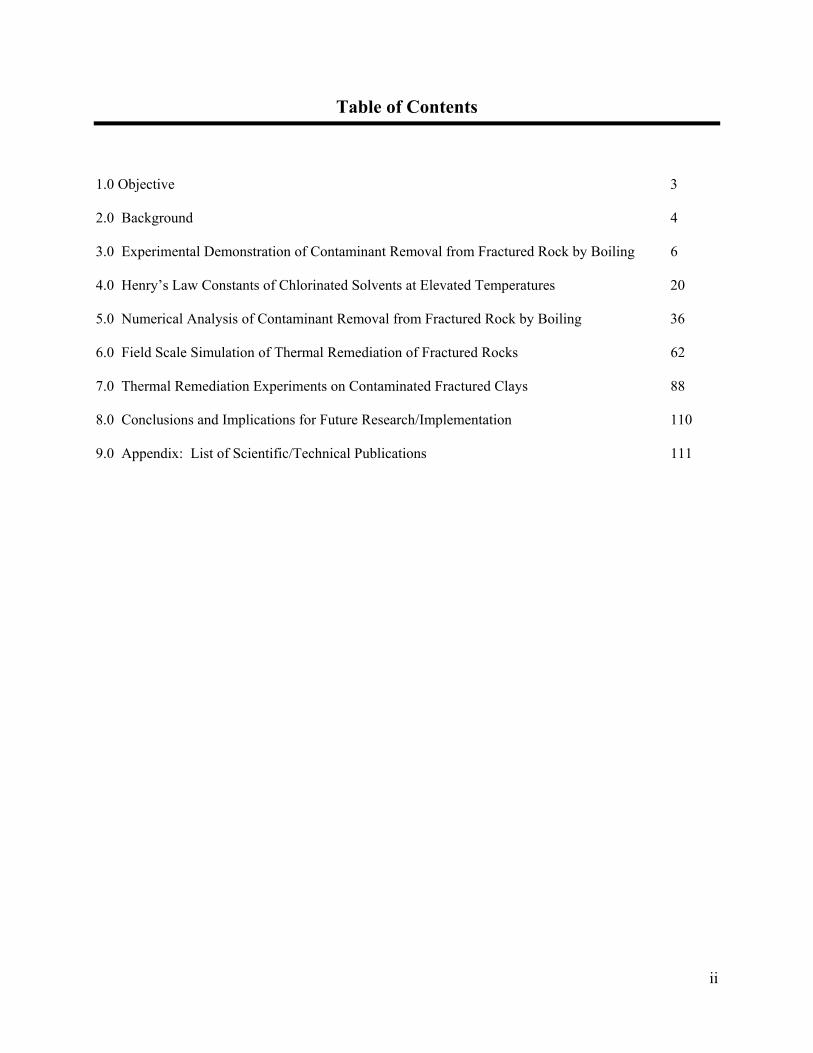
Table of Contents

1.0 Objective 3 2.0 Background 4 3.0 Experimental Demonstration of Contaminant Removal from Fractured Rock by Boiling 6 4.0 Henry’s Law Constants of Chlorinated Solvents at Elevated Temperatures 20 5.0 Numerical Analysis of Contaminant Removal from Fractured Rock by Boiling 36 6.0 Field Scale Simulation of Thermal Remediation of Fractured Rocks 62 7.0 Thermal Remediation Experiments on Contaminated Fractured Clays 88 8.0 Conclusions and Implications for Future Research/Implementation 110 9.0 Appendix: List of Scientific/Technical Publications 111

ii

List of Tables

Table 4.1 Measured Henry’s Law Constants at Various Temperatures 24

Table 4.2 Temperature Regressions of Henry’s Law Constants 26

Table 4.3 Aqueous Solubilities of Chlorinated Volatile Compounds 29

Table 4.4 Temperature Regression of Aqueous Solubility 33

Table 5.1 Values of material properties used in the simulation 39

Table 6.1 Capillary pressure and relative permeability 65

Table 7.1 Properties of clay 90

Table 7.2 Summary of three tests of heating clay matrix 93

Table 7.3 Summary of Test 3 103

iii

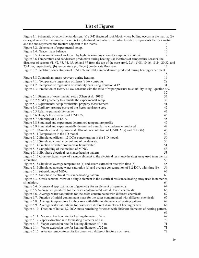
List of Figures Figure 3.1 Schematic of experimental design: (a) a 3-D fractured rock block where boiling occurs in the matrix; (b) enlarged view of a fracture-matrix set; (c) a cylindrical core where the unfractured core represents the rock matrix and the end represents the fracture adjacent to the matrix. 6 Figure 3.2. Schematic of experimental setup. 7 Figure 3.4. Tracer mass balance 10 Figure 3.5. Contamination of rock core by high pressure injection of an aqueous solution. 12 Figure 3.6 Temperature and condensate production during heating: (a) locations of temperature sensors, the distances of sensors #1, #2, #3, #4, #5, #6, and #7 from the top of the core are 0, 2.54, 5.08, 10.16, 15.24, 20.32, and 25.4 cm, respectively; (b) temperature profile; (c) condensate flow rate 13 Figure 3.7. Relative concentration of 1,2-DCA and NaBr in condensate produced during heating experiment. 15 Figure 3.8 Contaminant mass recovery during heating. 16 Figure 4.1. Temperature regression of Henry’s law constants. 28 Figure 4.2. Temperature regression of solubility data using Equation 4.12. 31 Figure 4.3. Prediction of Henry’s Law constant with the ratio of vapor pressure to solubility using Equation 4.9. 32 Figure 5.1 Diagram of experimental setup (Chen et al. 2010) 37 Figure 5.2 Model geometry to simulate the experimental setup. 38 Figure 5.3 Experimental setup for thermal property measurement. 41 Figure 5.4 Capillary pressure curve of the Berea sandstone core 42 Figure 5.5 Relative permeability curve 43 Figure 5.6 Henry’s law constants of 1,2-DCA. 45 Figure 5.7 Solubility of 1,2-DCA. 45 Figure 5.8 Simulated and experiment determined temperature profile 47 Figure 5.9 Simulated and experimentally determined cumulative condensate produced 48 Figure 5.10 Simulated and experimental effluent concentration of 1,2-DCA (a) and NaBr (b) 48 Figure 5.11 Temperature in the 1D model. 50 Figure 5.12 Simulated effluent 1,2-DCA concentration in the 1-D model. 50 Figure 5.13 Simulated cumulative volume of condensate. 50 Figure 5.14 Fraction of water produced as liquid water. 51 Figure 5.15 Subgridding of the method of MINC. 53 Figure 5.16 Six-phase electrical resistance heating pattern. 53 Figure 5.17 Cross-sectional view of a single element in the electrical resistance heating array used in numerical simulation. 53 Figure 5.18 Simulated average temperature (a) and steam extraction rate with time (b). 55 Figure 5.19 Simulated average water saturation (a) and average concentration of 1,2-DCA with time (b). 56 Figure 6.1. Subgridding of MINC. 63 Figure 6.2. Six-phase electrical resistance heating pattern. 63 Figure 6.3. Cross-sectional view of a single element in the electrical resistance heating array used in numerical simulation. 64 Figure 6.4. Numerical approximation of geometry for an element of symmetry. 64 Figure 6.5 Average temperatures for the cases contaminated with different chemicals 66 Figure 6.6. Average water saturations for the cases contaminated with different chemicals 67 Figure 6.7. Fraction of initial contaminant mass for the cases contaminated with different chemicals 67 Figure 6.8. Average temperatures for the cases with different diameters of heating pattern. 68 Figure 6.9. Average water saturations for cases with different diameters of heating pattern. 68 Figure 6.10. Fraction of initial 1,2-DCA mass remaining for cases with different diameters of heating pattern. 69 Figure 6.11. Vapor extraction rate for heating diameter of 4 m. 69 Figure 6.12 Vapor extraction rate for heating diameter of 8 m. 70 Figure 6.13. Vapor extraction rate for heating diameter of 16 m. 71 Figure 6.14. Vapor extraction rate for heating diameter of 32 m. 71 Figure 6.15. Average temperatures for the cases with different fracture apertures. 72

iv

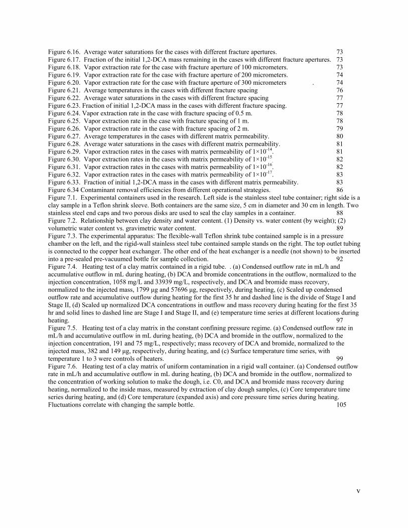
Figure 6.16. Average water saturations for the cases with different fracture apertures. 73 Figure 6.17. Fraction of the initial 1,2-DCA mass remaining in the cases with different fracture apertures. 73 Figure 6.18. Vapor extraction rate for the case with fracture aperture of 100 micrometers. 73 Figure 6.19. Vapor extraction rate for the case with fracture aperture of 200 micrometers. 74 Figure 6.20. Vapor extraction rate for the case with fracture aperture of 300 micrometers . 74 Figure 6.21. Average temperatures in the cases with different fracture spacing 76 Figure 6.22. Average water saturations in the cases with different fracture spacing 77 Figure 6.23. Fraction of initial 1,2-DCA mass in the cases with different fracture spacing. 77 Figure 6.24. Vapor extraction rate in the case with fracture spacing of 0.5 m. 78 Figure 6.25. Vapor extraction rate in the case with fracture spacing of 1 m. 78 Figure 6.26. Vapor extraction rate in the case with fracture spacing of 2 m. 79 Figure 6.27. Average temperatures in the cases with different matrix permeability. 80 Figure 6.28. Average water saturations in the cases with different matrix permeability. 81 Figure 6.29. Vapor extraction rates in the cases with matrix permeability of 1×10-14. 81 Figure 6.30. Vapor extraction rates in the cases with matrix permeability of 1×10-15

. 82 Figure 6.31. Vapor extraction rates in the cases with matrix permeability of 1×10-16. 82 Figure 6.32. Vapor extraction rates in the cases with matrix permeability of 1×10-17. 83 Figure 6.33. Fraction of initial 1,2-DCA mass in the cases with different matrix permeability. 83 Figure 6.34 Contaminant removal efficiencies from different operational strategies. 86 Figure 7.1. Experimental containers used in the research. Left side is the stainless steel tube container; right side is a clay sample in a Teflon shrink sleeve. Both containers are the same size, 5 cm in diameter and 30 cm in length. Two stainless steel end caps and two porous disks are used to seal the clay samples in a container. 88 Figure 7.2. Relationship between clay density and water content. (1) Density vs. water content (by weight); (2) volumetric water content vs. gravimetric water content. 89 Figure 7.3. The experimental apparatus: The flexible-wall Teflon shrink tube contained sample is in a pressure chamber on the left, and the rigid-wall stainless steel tube contained sample stands on the right. The top outlet tubing is connected to the copper heat exchanger. The other end of the heat exchanger is a needle (not shown) to be inserted into a pre-sealed pre-vacuumed bottle for sample collection. 92 Figure 7.4. Heating test of a clay matrix contained in a rigid tube. . (a) Condensed outflow rate in mL/h and accumulative outflow in mL during heating, (b) DCA and bromide concentrations in the outflow, normalized to the injection concentration, 1058 mg/L and 33939 mg/L, respectively, and DCA and bromide mass recovery, normalized to the injected mass, 1799 μg and 57696 μg, respectively, during heating, (c) Scaled up condensed outflow rate and accumulative outflow during heating for the first 35 hr and dashed line is the divide of Stage I and Stage II, (d) Scaled up normalized DCA concentrations in outflow and mass recovery during heating for the first 35 hr and solid lines to dashed line are Stage I and Stage II, and (e) temperature time series at different locations during heating. 97 Figure 7.5. Heating test of a clay matrix in the constant confining pressure regime. (a) Condensed outflow rate in mL/h and accumulative outflow in mL during heating, (b) DCA and bromide in the outflow, normalized to the injection concentration, 191 and 75 mg/L, respectively; mass recovery of DCA and bromide, normalized to the injected mass, 382 and 149 μg, respectively, during heating, and (c) Surface temperature time series, with temperature 1 to 3 were controls of heaters. 99 Figure 7.6. Heating test of a clay matrix of uniform contamination in a rigid wall container. (a) Condensed outflow rate in mL/h and accumulative outflow in mL during heating, (b) DCA and bromide in the outflow, normalized to the concentration of working solution to make the dough, i.e. C0, and DCA and bromide mass recovery during heating, normalized to the inside mass, measured by extraction of clay dough samples, (c) Core temperature time series during heating, and (d) Core temperature (expanded axis) and core pressure time series during heating. Fluctuations correlate with changing the sample bottle. 105

v

Acronyms CF Chloroform CT Carbon Tetrachloroethylene CVOC Chlorinated Volatile Organic Compounds DCA Dichloroethane DDI Distilled Deionized DNAPL Dense Nonaqueous Phase Liquid ECD Electron Capture Detector EDB Dibromethane EPICS Equilibrium Partitioning In Closed Systems FID Flame Ionized Detector GC Gas Chromatography IC Ion Chromatography MCL Maximum Contaminant Levels MINC Multiple Interacting Continua NAPL NonAqueous Phase Liquid PCE Tetrachloroethylene RTD Resistive Thermal Detectors TCE Trichloroethylene USEPA U.S. Environmental Protection Agency VOC Volatile Organic Compounds

vi

vii

Acknowledgements The research upon which this report is based was a joint effort between the Clemson University Department of Environmental Engineering and Earth Sciences and the Strategic Environmental Research and Development Program (SERDP, project ER-1553). The research team would like to extend appreciation to the Executive Director of SERDP, Dr. Jeff Marqusee, and the SERDP Environmental Restoration Program Manager, Dr. Andrea Leeson, for their support.

Abstract

The DoD is responsible for cleanup of groundwater that is contaminated with chlorinated volatile organic compounds (CVOC) at thousands of sites. Many of these sites are underlain by fractured rocks or soils with significant matrix porosity. As dissolved CVOC and dense nonaqueous phase liquids (DNAPL) move through fracture networks, the CVOC diffuse into the lower permeability matrix materials, where they can remain for hundreds of years. Remediation options for treating fractured geologic media are extremely limited because the low matrix permeability, and unknown fracture locations make any type of fluid or chemical delivery difficult or impossible.

Thermal methods hold promise for remediation of fractured media, because heat can be efficiently transferred without any fluid flow by the mechanisms of thermal conduction and electrical resistance heating. Once a fractured rock or soil is heated above the water boiling point, subsequent depressurization of the fracture network by vacuum extraction may induce boiling in the matrix, leading to large gas phase pressure gradients, and a steam stripping effect that can remove the contaminants from the matrix.

Objectives. The objectives of this work were to 1) experimentally and theoretically evaluate the contaminant mass removal process from heated low permeability matrix materials that are bounded by a depressurized fracture network; 2) assess the feasibility of field scale implementation of thermal remediation techniques at fractured sites, and 3) develop design and operational strategies for maximizing the effectiveness of field scale applications of thermal remediation methods at fracture sites.

Technical Approach. The research used an integrated bench scale experimental and numerical modeling approach. The primary fluid, heat, and contaminant transport processes during matrix boiling and fracture depressurization occur at the scale of a single matrix block. The laboratory tests consisted of heating contaminated low permeability rocks and soil cores to temperatures above the normal boiling point, and depressurizing a fracture at one end of a sealed column. Temperature, steam discharge, and contaminant recovery data from the cores during boiling were collected, and used to assess the phenomena. A multiphase heat and mass transfer numerical model was used to analyze the experiments, and to evaluate the boiling and contaminant mass transfer over a wider range of fractured porous media characteristics

Results. Key findings of this work are that CVOC are readily removed from low to moderate permeability fractured materials through the boiling mechanism, and it is not necessary to boil all of the pore water to get complete contaminant removal by this mechanism. Simulation results show that remediation efficiency is sensitive to the amount of heat added to the system; in some case the addition of a relatively small additional amount of heat can greatly improve the remediation efficiency. The contaminant recovery from fractured rock masses in simulations was relatively insensitive to the fracture properties, assuming that the fractures are continuous and well-connected. The simulations were sensitive to the unfractured matrix permeability, with lower permeability corresponding to somewhat lower removal efficiencies for a given thermal

1

input. However, at higher thermal input, even the low permeability matrix simulations showed effective remediation.

Benefits. This project confirms the ability of thermal remediation to remove volatile contaminants from the matrix in fractured geologic media. The experimental and numerical methods developed here should be helpful in the future design and analysis of thermal remediation projects at fractured sites.

2

1.0 Objective

The purpose of this research was to better understand the coupled multiphase heat and mass transfer processes that occur in contaminated low permeability matrix materials when they are heated and then depressurized by an adjacent fracture. The work consisted of a series of laboratory column matrix boiling experiments, in which a fracture at the end of a sealed column was depressurized. The experimental work was integrated with numerical analyses of the multiphase heat and mass transfer phenomena that take place during the fracture-matrix boiling process. The specific objectives were to:

• Experimentally demonstrate the contaminant mass removal process from heated low

permeability matrix materials that are adjacent to depressurized fractures • Understand the local-scale controlling mechanisms for matrix boiling and

contaminant mass transfer using both laboratory experiments and numerical simulations with a variety of soil and rock matrix materials

• Assess the feasibility of field scale implementation of thermal remediation techniques at fractured sites, identifying key site characteristics that can help or limit the process

• Develop design and operational strategies for maximizing the effectiveness of field scale applications of thermal remediation methods at fractured sites.

3

2.0 Background

CVOC that diffuse into the low permeability rock matrix in a fractured rock site may cause long-term groundwater pollution and difficulties in cleanup. When CVOC are released, and the dissolved CVOC and DNAPL move through fractures, the sharp concentration distinction between fracture and matrix will result in rapid diffusion of CVOCs into the low permeability rock matrix [Parker et al., 1994; Parker et al., 1997; Ross and Lu, 1999; Slough et al., 1999; Esposito and Thomson, 1999; O’Hara et al., 2000; Reyonlds and Kueper, 2001; Falta, 2005; Reynolds and Kueper, 2002] . A significant amount of dissolved and adsorbed contaminant mass will be stored in the matrix over time, serving as a reservoir of contaminants. When the contaminants in fractures are removed by engineered or natural processes, contaminants in the matrix continuously diffuse back into the water flowing through the fractures. This may result in aqueous contaminant concentrations several orders of magnitude higher than the maximum contaminant levels (MCL). Without treatment, this process could last for hundreds of years[Parker et al., 1997; Slough et al., 1999; Falta, 2005; Reynolds and Kueper, 2002] serving as a long-term source for groundwater contamination. Remediation of fractured sites is challenging using isothermal methods such as air sparging, pump and treat, and chemical oxidation. Due to the low matrix permeability, it is difficult to flush the system with any type of fluid [Falta, 2005; Baston, 2008]. The uncertainty of fracture networks makes it even more difficult to reliably deliver remediation agents into the matrix [NRC, 1994; Goldstein et al., 2004; Mundle et al., 2007].

Thermal methods hold promise for remediating fractured geologic media. Heat can be successfully transferred to the rock matrix by thermal conduction [Ochs et al., 2003; Gudbjerg et al., 2004; heron et al., 2009], electrical resistive heating [Gauglitz et al., 1994; Heron et al., 2005] or radio-frequency heating [Roland et al., 2008; Kawala and Atamanczuk, 1998]. As fractured rock or soil is heated above the water boiling point, subsequent depressurization will induce boiling in the matrix. When boiling occurs, one volume of liquid water turns into about 1600 volumes of steam vapor at atmospheric pressure, resulting in high pressure gradients and steam volumetric flux. The portion of contaminant dissolved in water in the matrix will preferentially partition into the steam due to the increased Henry’s law constant at steam temperature [Heron et al., 1998], which is approximately 10 times higher than at ground water temperature for CVOC. This in-situ boiling may be an extremely effective mechanism for CVOC removal. Assuming batch conditions, Udell et al. (1998), Udell, (1996) and Heron et al. (1998) calculated that boiling away one percent of the water mass could theoretically lead to decrease of dissolved trichloroethylene (TCE) concentration by tens of orders of magnitude.

Contaminant mass transfer in fractured media due to in-situ boiling is not well understood. Some previous field studies showed some good removal rate when heating to above the water boiling temperature [Gauglitz et al., 1994]. Heron et al. (1998) examined TCE removal from a partially saturated (water saturation of 0.90) unfractured low permeability silt in the laboratory. When the temperature in the tank reached 99°C, boiling started, and the TCE removal rate was about 20 times higher than the initial removal rate. At the termination of the experiment, about 99.8% of the initial TCE mass was removed from the silt [Heron et al., 1998]. However, it is not clear where the boiling occurred in this study, though the removal of contaminant was linked to the in-situ boiling that was induced.

4

The contaminant mass transfer in fractured media due to boiling is anticipated to be a complex phenomenon. When boiling occurs in fractured media, there are strong couplings between convective and conductive heat transfer, multiphase flow and thermodynamics. Recently, Baston et al., (2011) found that fracture and rock matrix properties have significant influence on the heating time to remove all liquid water in the treatment zone. The detail of boiling phase change is important for contaminant mass transfer during this process because it is this phase change that strips the volatile contaminant from the liquid phase. Depending on conditions, the majority of boiling phase change could occur near fractures, or in the matrix. Some early studies on geothermal reservoirs showed that boiling could be induced in the matrix provided that matrix permeability is larger than about 1×10-17 m2 [Pruess, 1983]. When this is the case, the vapor phase moves from boiling locations in the matrix to the fracture. When the permeability less than about 1×10-17 m2, the liquid phase moves from the matrix to the fracture and boiling occurs mainly in the fracture [Pruess, 1983]. The efficiency of contaminant removal in these two scenarios would vary greatly due to the presence or absence of steam stripping by the vapor phase in the matrix. Understanding the mechanism of mass transfer due to in-situ boiling in fractured porous media helps to evaluate the remediation feasibility, and develop design and operational strategies for maximizing the effectiveness of thermal remediation in fractured media.

5

Methods and Results

This section is based on five journal paper manuscripts related to this project that have been published, submitted for publication, or are about to be submitted for publication. We have organized this overall section to describe the methods and results for each major component of the research

3. Experimental Demonstration of Contaminant Removal from Fractured Rock by Boiling (published in Environmental Science and Technology, Vol. 44, No. 16, 6437-6442, 2010)

3.1 Introduction

The purpose of this study was to demonstrate removal of CVOC from fractured rocks by in-situ boiling. Following Figure 3.1., an unfractured cylindrical rock core was used to represent the fracture-matrix system at its most fundamental level. With this setup, the open end of the rock core represents the fracture adjacent to the rock matrix.

Figure 3.2. Schematic of experimental design: (a) a 3-D fractured rock block where boiling occurs in the matrix; (b) enlarged view of a fracture-matrix set; (c) a cylindrical core where the unfractured core represents the rock matrix and the end represents the fracture adjacent to the matrix.

6

3.2 Experimental section

3.2.1 Apparatus

The apparatus (Figure 3.2) is primarily composed of a core assembly, pressurized vessel, condenser, circulation system, temperature control and data acquisition systems.

Core preparation. The core assembly is made up of a cylindrical unfractured rock sample (5.08×30.48 cm), two aluminum endcaps, porous disks, a Teflon shrink tube, thermistors, resistive thermal detectors (RTD), heaters and an insulation layer. A Berea sandstone core with a hydraulic permeability of 2×10-13 m2 and porosity of 0.174 was obtained from Cleveland, Ohio. This rock core is used to represent the rock matrix with the top end representing the fracture adjacent to matrix (Figure 3.2). The system is designed so that the core may be contaminated by water circulation at high pressure. During heating tests, only the top end of the core is open, to simulate a depressurized fracture.

Figure 3.2. Schematic of experimental setup.

7

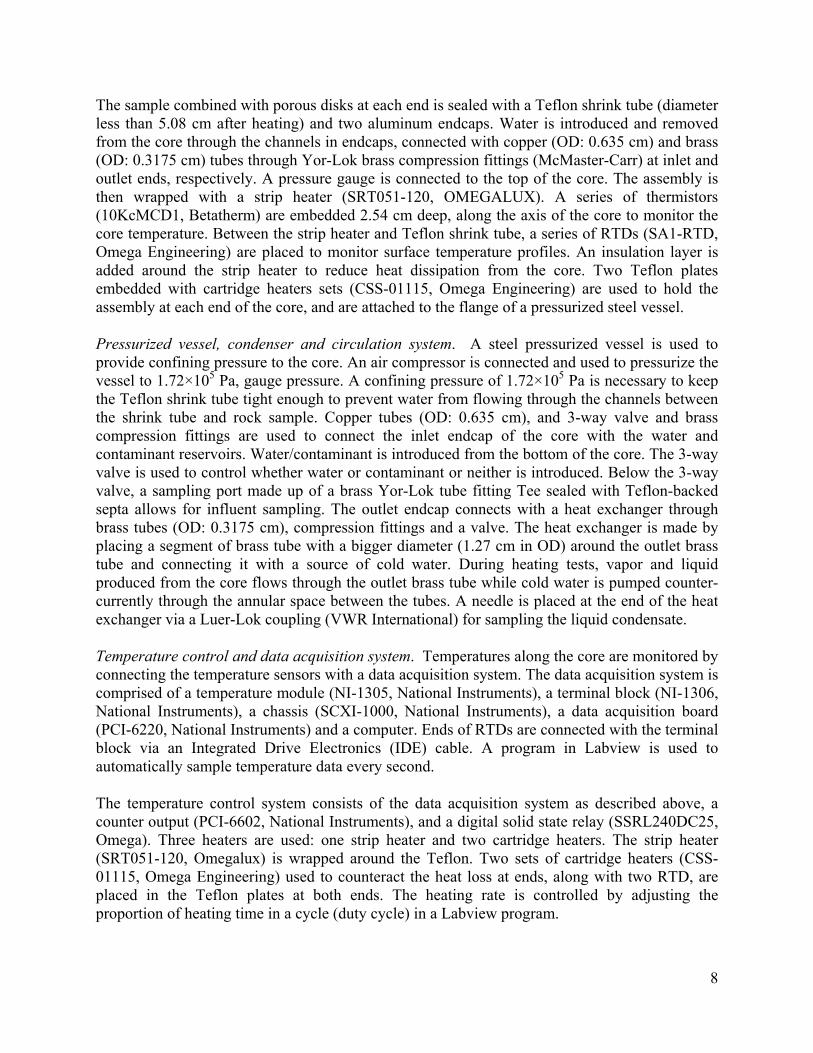
The sample combined with porous disks at each end is sealed with a Teflon shrink tube (diameter less than 5.08 cm after heating) and two aluminum endcaps. Water is introduced and removed from the core through the channels in endcaps, connected with copper (OD: 0.635 cm) and brass (OD: 0.3175 cm) tubes through Yor-Lok brass compression fittings (McMaster-Carr) at inlet and outlet ends, respectively. A pressure gauge is connected to the top of the core. The assembly is then wrapped with a strip heater (SRT051-120, OMEGALUX). A series of thermistors (10KcMCD1, Betatherm) are embedded 2.54 cm deep, along the axis of the core to monitor the core temperature. Between the strip heater and Teflon shrink tube, a series of RTDs (SA1-RTD, Omega Engineering) are placed to monitor surface temperature profiles. An insulation layer is added around the strip heater to reduce heat dissipation from the core. Two Teflon plates embedded with cartridge heaters sets (CSS-01115, Omega Engineering) are used to hold the assembly at each end of the core, and are attached to the flange of a pressurized steel vessel.

Pressurized vessel, condenser and circulation system. A steel pressurized vessel is used to provide confining pressure to the core. An air compressor is connected and used to pressurize the vessel to 1.72×105 Pa, gauge pressure. A confining pressure of 1.72×105 Pa is necessary to keep the Teflon shrink tube tight enough to prevent water from flowing through the channels between the shrink tube and rock sample. Copper tubes (OD: 0.635 cm), and 3-way valve and brass compression fittings are used to connect the inlet endcap of the core with the water and contaminant reservoirs. Water/contaminant is introduced from the bottom of the core. The 3-way valve is used to control whether water or contaminant or neither is introduced. Below the 3-way valve, a sampling port made up of a brass Yor-Lok tube fitting Tee sealed with Teflon-backed septa allows for influent sampling. The outlet endcap connects with a heat exchanger through brass tubes (OD: 0.3175 cm), compression fittings and a valve. The heat exchanger is made by placing a segment of brass tube with a bigger diameter (1.27 cm in OD) around the outlet brass tube and connecting it with a source of cold water. During heating tests, vapor and liquid produced from the core flows through the outlet brass tube while cold water is pumped counter-currently through the annular space between the tubes. A needle is placed at the end of the heat exchanger via a Luer-Lok coupling (VWR International) for sampling the liquid condensate.

Temperature control and data acquisition system. Temperatures along the core are monitored by connecting the temperature sensors with a data acquisition system. The data acquisition system is comprised of a temperature module (NI-1305, National Instruments), a terminal block (NI-1306, National Instruments), a chassis (SCXI-1000, National Instruments), a data acquisition board (PCI-6220, National Instruments) and a computer. Ends of RTDs are connected with the terminal block via an Integrated Drive Electronics (IDE) cable. A program in Labview is used to automatically sample temperature data every second.

The temperature control system consists of the data acquisition system as described above, a counter output (PCI-6602, National Instruments), and a digital solid state relay (SSRL240DC25, Omega). Three heaters are used: one strip heater and two cartridge heaters. The strip heater (SRT051-120, Omegalux) is wrapped around the Teflon. Two sets of cartridge heaters (CSS-01115, Omega Engineering) used to counteract the heat loss at ends, along with two RTD, are placed in the Teflon plates at both ends. The heating rate is controlled by adjusting the proportion of heating time in a cycle (duty cycle) in a Labview program.

8

3.2.2 Chemicals, sample collection and analytical techniques

Chemicals used in this test are 1,2-dichloroethane (1,2-DCA) (Analytical grade, Mallinckrodt), NaBr (Analytical grade, Mallinckrodt). The selection of 1,2-DCA as the model compound is because it was frequently found in contamination sites [Henderson et al., 2008]; most importantly, it has similar physical properties as other chlorinated solvents such as TCE, but relatively high solubility and less volatility, which minimize loss from evaporation during experiment. NaBr was used as a tracer because it is non-volatile and conservative.

Effluent samples were collected at the end of the heat exchanger using 10-mL glass vials sealed with Teflon-backed septa. About 2mL of air was pre-extracted from each vial using a graduated syringe to reduce pressure buildup during sampling. The weight of the sealed vial is recorded as W1. The sample is taken by plugging the sealed vial to the outlet needle and pulling out the vial after about 2mL of sample is collected. The weight of the vial with sample is recorded as W2. The mass of sample (Ws) was calculated as Ws=W2-W1. Influent samples were collected at the sampling port below the 3-way valve. About 2 mL of influent sample was collected with a graduated syringe and transferred to a partially vacuumed vial. The mass of sample was obtained by weighing the vial with and without sample.

The aqueous concentration of 1,2-DCA was quantified by head space analysis using a 5890 series II Plus Hewlett-Packard gas chromatograph (GC), equipped with a flame ionization detector (FID). Samples were filtered with 0.2-μm-pore-size PTFE syringe filters (VWR International). Bromide was measured from filtered samples with a Dionex ion chromatograph (IC) with an AS11/AG11 column. The eluant for bromide determination is carbonate (4.5mM) and bicarbonate (0.8mM).

3.2.3 Experimental procedures

Saturating the sample. The rock sample was saturated with water by first circulating CO2 gas at a low rate to remove air from the core. De-aired water was then pumped through the core from bottom to top at 6.89×104 Pa (gauge pressure), until the inlet flow rate equaled to the outlet flow rate.

Dissolved tracer test. A tracer test was conducted after the core was water saturated. A 132 mL solution containing 108 mg/L sodium bromide (NaBr), and 255 mg/L 1,2-dichloroethane (1,2-DCA) was injected. Samples were collected at the outlet, and the volume of effluent produced was recorded. Concentrations of 1,2-DCA and bromide were measured using GC and IC, respectively.

Heating Test. The water saturated rock sample was contaminated by injecting an aqueous solution containing 1,2-DCA (253 mg/L), and NaBr (144 mg/L) through the sample. Both the influent and the effluent concentrations, and the volume of water circulated were monitored. Both inlet and outlet valves were closed when the effluent 1,2-DCA and NaBr concentrations stabilized. The amounts of 1,2-DCA and NaBr mass remaining in the core are calculated by substracting the mass removed from the core from the mass injected.

9

A constant power input of 31.3 watts was applied with the strip heater. The power inputs of cartridge heaters at each end were adjusted to counteract the heat loss at the ends, ranging from 1.2 watts to 15 watts. Due to thermal expansion of fluid and possible noncondensible gas trapped in the pore, the core pressure increased during the heating process prior to boiling. It was released by quickly opening and shutting the outlet valve as the gauge pressure exceeded about 1.03×105 Pa.

The outlet valve was opened when the surface temperature exceeded 100 °C. Steam generated from boiling was condensed to liquid in the heat changer. The condensate was collected at the outlet by plugging in sealed and partially vacuumed vials. The volume of condensate produced was recorded, and concentrations of 1,2-DCA and NaBr in the condensate were measured by GC and IC analysis, respectively.

3.3 Results and discussion

3.3.1 Tracer Test

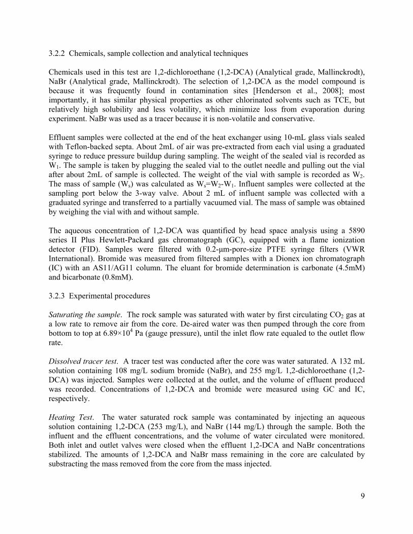
The tracer test was conducted by injecting a pulse of 132mL of water with NaBr at 108 mg/L, and 1,2-DCA at 255 mg/L followed by water. The influent and effluent concentrations of 1,2-DCA, CB and NaBr were plotted as a function of water produced from the core (Figure 3.3). Bromide was produced after circulating approximately the fluid volume of pores (104 mL) and tubes (25mL), indicating that water flows axially through the core without short circuiting. 1,2-DCA breakthrough follows the bromide, flowing out after circulating 118 mL of water, indicating only slight adsorption of the 1,2-DCA. This is consistent with its low Koc of 33. 27

Figure 3.3. Tracer breakthrough curves.

Volume of water produced (ml)

0.0

0.2

0.4

0.6

0.8

1.01,2-DCANaBr

Cou

t/Cin

0 200 400 600 800

10

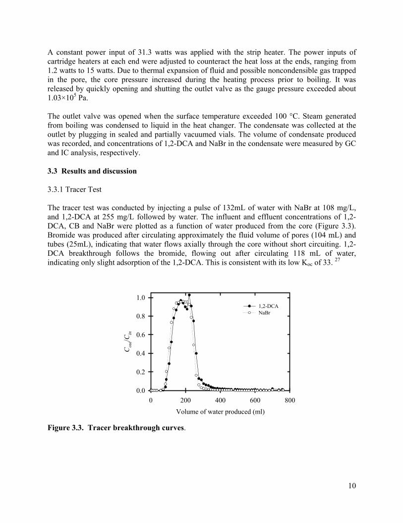
A mass balance on the tracer test was conducted by integrating the area under the curves in Figure 3.3. The ratio of cumulative effluent mass to the total mass injected is presented in Figure 3.4. The recovery of 1,2-DCA and NaBr in this tracer test were 98% and 93%, respectively. The high recovery of mass suggests that there is little leakage or other source of mass loss from the system during sampling and analysis.

0.0

0.2

0.4

0.6

0.8

1.0

Figure 3.4. Tracer mass balance.

3.3.2 Contamination of the Core

Before the heating test, the core was contaminated by injecting 1,2-DCA and NaBr dissolved in water. To uniformly contaminate the core, 350 mL of 1,2-DCA (253 mg/L), and NaBr (144 mg/L) were injected under high pressure (6.89×104 Pa, gauge). Both inlet and outlet concentrations were monitored, and the results are shown in Figure 3.5. Initially, the 1,2-DCA and NaBr concentrations in the core were nearly zero. After injecting 350 mL of solution, effluent concentrations stabilized and both inlet and outlet valves were then closed. The masses of 1,2-DCA and NaBr remaining in the core were 26.9 mg and 15.3 mg, respectively.

3.3.3 Temperature Profile and Condensate Flow during Heating

After the core was uniformly contaminated, both inlet and outlet valves were closed, and the heaters were turned on. Condensate samples were collected over time until no more condensate was produced. The heaters were shut off after the core started drying out.

Core temperatures were monitored using sensors embedded 2.54 cm deep in the core (Figure a). The distances away from the top (outlet) end the core are 0, 2.54, 5.08, 10.16, 15.24, 20.32, and 25.4 cm. From top to bottom, they are labeled as #1, #2, #3, #4, #5, #6 and #7. Before the outlet valve was opened, the core was uniformly heated and the temperature increased gradually; when

Volume of water produced (ml)

Cum

ulat

ive

mas

s out

/mas

s in

1,2-DCANaBr

0 200 400 600 800

11

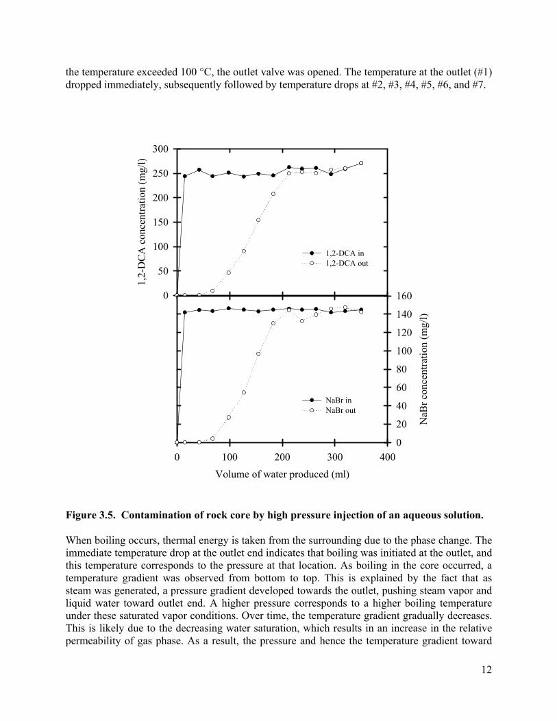
the temperature exceeded 100 °C, the outlet valve was opened. The temperature at the outlet (#1) dropped immediately, subsequently followed by temperature drops at #2, #3, #4, #5, #6, and #7.

0

50

100

150

200

250

300

1,2-

DC

A c

once

ntra

tion

(mg/

l)

1,2-DCA in

1,2-DCA out

0

20

40

60

80

100

120

140

160

Figure 3.5. Contamination of rock core by high pressure injection of an aqueous solution.

When boiling occurs, thermal energy is taken from the surrounding due to the phase change. The immediate temperature drop at the outlet end indicates that boiling was initiated at the outlet, and this temperature corresponds to the pressure at that location. As boiling in the core occurred, a temperature gradient was observed from bottom to top. This is explained by the fact that as steam was generated, a pressure gradient developed towards the outlet, pushing steam vapor and liquid water toward outlet end. A higher pressure corresponds to a higher boiling temperature under these saturated vapor conditions. Over time, the temperature gradient gradually decreases. This is likely due to the decreasing water saturation, which results in an increase in the relative permeability of gas phase. As a result, the pressure and hence the temperature gradient toward

Volume of water produced (ml)

NaB

r con

cent

ratio

n (m

g/l)

NaBr inNaBr out

0 100 200 300 400

12

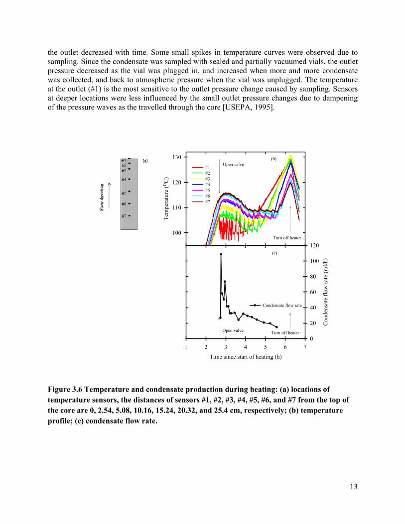
the outlet decreased with time. Some small spikes in temperature curves were observed due to sampling. Since the condensate was sampled with sealed and partially vacuumed vials, the outlet pressure decreased as the vial was plugged in, and increased when more and more condensate was collected, and back to atmospheric pressure when the vial was unplugged. The temperature at the outlet (#1) is the most sensitive to the outlet pressure change caused by sampling. Sensors at deeper locations were less influenced by the small outlet pressure changes due to dampening of the pressure waves as the travelled through the core [USEPA, 1995].

100

110

120

130

Figure 3.6 Temperature and condensate production during heating: (a) locations of temperature sensors, the distances of sensors #1, #2, #3, #4, #5, #6, and #7 from the top of the core are 0, 2.54, 5.08, 10.16, 15.24, 20.32, and 25.4 cm, respectively; (b) temperature profile; (c) condensate flow rate.

Tem

pera

ture

(oC

)#1#2#3#4#5#6#7

Time since start of heating (h)1 2 3 4 5 6 7

Con

dens

ate

flow

rate

(ml/h

)

0

20

40

60

80

100

120

Condensate flow rate

Open valve

Turn off heater

Open valve Turn off heater

(b)

(c)

13

At later times, the outlet (#1) temperature began to increase as the liquid water boiled away, and superheated vapor conditions prevailed. Subsequently the temperatures at locations #2, #3, #4, #5, #6, and #7 increased as these zones dried out. After approximately 6.3 hours, the heater was turned off and the temperature started decreasing.

Steam (a mixture of liquid and vapor) coming out of the core was condensed and the condensate flow rate with time was plotted (Figure b). A large amount of condensate was generated right after the valve was opened, but as will be explained, some of this exited the core as a liquid phase. The flow rate increased to 108.6 mL/h, and gradually dropped to about 14.79 mL/h. After about 5.56 hours of heating, the core dried out, which corresponds to the temperature increases at the bottom of the core.

3.3.4 Contaminant Removal Due to Boiling

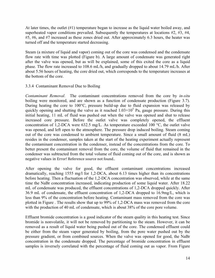
Contaminant Removal. The contaminant concentrations removed from the core by in-situ boiling were monitored, and are shown as a function of condensate production (Figure 3.7). During heating the core to 100°C, pressure build-up due to fluid expansion was released by quickly opening and shutting the valve as it reached 1.03×105 Pa, gauge pressure. During this initial heating, 11 mL of fluid was pushed out when the valve was opened and shut to release increased core pressure. Before the outlet valve was completely opened, the effluent concentration of 1,2-DCA were 632.5 mg/L. As temperature exceeded 100 °C, the outlet valve was opened, and left open to the atmosphere. The pressure drop induced boiling. Steam coming out of the core was condensed to ambient temperature. Since a small amount of fluid (8 mL) resides in the condenser, samples taken at the start of the heating experiment actually represent the contaminant concentration in the condenser, instead of the concentrations from the core. To better present the contaminant removal from the core, the volume of fluid that remained in the condenser was subtracted from the total volume of fluid coming out of the core, and is shown as negative values in Error! Reference source not found..

After opening the valve for good, the effluent contaminant concentrations increased dramatically, reaching 1555 mg/l for 1,2-DCA, about 6.13 times higher than its concentrations before heating. Then a fluctuation of the 1,2-DCA concentration was observed, while at the same time the NaBr concentration increased, indicating production of some liquid water. After 18.22 mL of condensate was produced, the effluent concentrations of 1,2-DCA dropped quickly. After 36.9 mL of condensate, the effluent concentration of 1,2-DCA dropped to 16.9mg/L, which is less than 9% of the concentration before heating. Contaminant mass removed from the core was plotted in Figure . The results show that up to 99% of 1,2-DCA mass was removed from the core with the production of 40 mL of condensate, which is about 38% of the core pore volume.

Effluent bromide concentration is a good indicator of the steam quality in this heating test. Since bromide is nonvolatile, it will not be removed by partitioning to the steam. However, it can be removed as a result of liquid water being pushed out of the core. The condensed effluent could be either from the steam vapor generated by boiling, from the pore water pushed out by the pressure gradient, or from combined sources. When the valve was opened for good, the NaBr concentration in the condensate dropped. The percentage of bromide concentration in effluent samples is inversely correlated with the percentage of fluid coming out as vapor. From Figure

14

3.7, one can see that the bromide concentration dropped greatly after the valve was opened, which as a result corresponds to a period of high contaminant removal. Then an increase of the percentage of bromide corresponds to the decrease of contaminant concentration removed from the core. Further decrease of the bromide concentration corresponds to another peak of contaminant concentration. Bromide concentration approached zero when approximately 50 mL condensate (about 48% pore volume) was produced, indicating that the condensate was 100% vapor when it left the core.

0

2

4

6 1,2-DCA

Cou

t/Cin

Figure 3.7. Relative concentration of 1,2-DCA and NaBr in condensate produced during heating experiment.

Volume of condensate produced (ml)0 20 40 60 80 100

Cou

t/Cin

0.0

0.2

0.4

0.6

0.8

1.0Open valve

NaBr

Open valve

15

0.0

0.2

0.4

0.6

0.8

1.0

Figure 3.8 Contaminant mass recovery during heating.

3.4 Summary

In summary, thermal removal of chlorinated solvents from a sandstone rock matrix was experimentally demonstrated in the laboratory. After the core was contaminated with 1,2-DCA, heating the core above 100 °C and subsequently opening one end of the core to the atmosphere induced boiling in the core. As boiling occurred in the core, a temperature gradient towards the outlet was observed, indicating that steam was generated and a pressure gradient developed towards the outlet, pushing steam vapor and liquid water out of the core. As boiling occurred, the effluent concentration of 1,2-DCA peaked up to 6.1 times higher than before being heated. The 1,2-DCA was quickly removed from the matrix due to in-situ boiling. When 38% of the pore volume of condensate was produced, nearly 100% 1,2-DCA was recovered. Non-volatile bromide concentration in condensate is a good indicator of the percentage of water coming out as liquid water. Combined with the 1,2-DCA concentrations curve, it shows that a higher percentage of condensate coming out as vapor corresponds to more concentrated 1,2-DCA removal from the core. This demonstrates that the chlorinated volatile compound is primarily removed by partitioning to vapor phase flow.

Volume of condensate produced (ml)0 20 40 60 80 100

Acc

umul

aou

tot

Mal

/T

tive

M

1,2-DCA

Open valve

16

3.5. References

Baston, D. P. Analytical and numerical modelling of thermal conductive heating in fractured rock. Queen's University, Kingston, Ontario, Canada, 2008.

Baston, D. P.; Falta, R. W.; Kueper, B. H., Numerical modeling of thermal conductive heating in fractured bedrock. Journal of Ground Water in print.

Espositio, S. J.; Thomson, N. R., Two-phase flow and transport in a single fracture-porous medium system. Journal of Contaminant Hydrology 1999, 37, 319-341.

EPA, National primary drinking water regulations. In Contaminant specific fact sheets Volatile Organic Chemicals, Technical Version ed.; USEPA, Ed. Office of Water: 1995.

Falta, R. W., Dissolved chemical discharge from fractured clay aquitards contaminated by DNAPLs. In Dyanmics of Fluids in Fractured Rocks, Faybishenko, B.; Witherspoon, P. A.; Gale, J., Eds. American Geolophysical Union: San Francisco, 2005; Vol. 162.

Gauglitz, P. A.; Roberts, J. S.; Bergsman, T. M.; Schalla, R.; Caley, S. M.; Schlender, M. H.; Heath, W. O.; Jarosch, T. R.; Miller, M. C.; Eddy-Dilek, C. A.; Moss, R. W.; Looney, B. B. Six-phase soil heating for enhanced removal of contaminants: Volatile organic compounds in non-arid soils integrated demonstration, Savannah River Site; Pacific Northwest Laboratory: Richland, Washington, 1994; pp 325-339.

Goldstein, K. J.; Vitolins, A. R.; Navon, D.; Parker, B. L.; Chapman, S.; Anderson, G. A., Characterization and pilot-scale studies for chemical oxidation remediation of fractured shale. Remediation 2004, 14, (4), 19-37.

Gudbjerg, J.; Sonnenborg, T. O.; Jensen, K. H., Remediation of NAPL below the water table by steam-induced heat conduction. Journal of Contaminant Hydrology 2004, 72, (1-4), 207-225.

Henderson, J. K.; Freedman, D. L.; Falta, R. W.; Kuder, T.; Wilson, J. T., Anaerobic biodegradation of ethylene dibromide and 1,2-dichloroethane in the presence of fuel hydrocarbons. Environmental Science & Technology 2008, 42, (3), 864-870.

Heron, G.; Christensen, T. H.; Enfield, C. G., Henry's law constant for trichloroethylene between 10 and 95 οC. Environmental Science & Technology 1998, 32, (10), 1433-1437.

Heron, G.; Parker, K.; Galligan, J.; Holmes, T. C., Thermal treatment of eight CVOC source zones to near nondetect concentrations. Ground Water Monitoring & Remediation 2009, 29, (3), 56-65.

Heron, G.; Carroll, S.; Nielsen, S. G., Full-scale removal of DNAPL constituents using steam-enhanced extraction and electrical resistance heating. Ground Water Monitoring and Remediation 2005, 25, (4), 92-107.

17

Heron, G.; Zutphen, M. V.; Christensen, T. H.; Enfield, C. G., Soil heating for enhanced remediation of chlorinated solvents: A laboratory study on resistive heating and vapor extraction in a silty, low-permeable soil contaminated with trichloroethylene. Environmental Science and Technology 1998, 32, (10), 1474-1481.

Kawala, Z.; Atamanczuk, T., Microwave-enhanced thermal decontamination of soil. Environmental Science & Technology 1998, 32, (17), 2602-2607.

Mundle, K.; Reynolds, D. A.; West, M. R.; Kueper, B. H., Concentration rebound following in situ chemical oxidation in fractured clay. Groundwater 2007, 45, (6), 692-702.

National Research Council, Alternatives for Ground Water Cleanup. National Academy Press: Washington D.C., 1994.

Ochs, S. O.; Hodges, R. A.; Falta, R. W.; Kmetz, T. F.; Kupar, J. J.; Brown, N. N.; Parkinson, D. L., Predicted heating patterns during steam flooding of coastal plain sediments at the Savannah River Site. Environmental & Engineering Geoscience 2003, 9, (1), 51-69.

O'Hara, S. K.; Parker, B. L.; Jorgensen, P. R.; Cherry, J. A., Trichloroethene DNAPL flow and mass distribution in naturally fractured clay: Evidence of aperture variability. Water Resources Research 2000, 36, (1), 135-147.

Parker, B. L.; McWhorter, D. B.; Cherry, J. A., Diffusive disappearance of immiscible-phase organic liquids in fractured geologic media. Groundwater 1994, 32, (4), 805-820.

Parker, B. L.; McWhorter, D. B.; Cherry, J. A., Diffusive loss of non-aqueous phase organic solvents from idealized fracture networks in geologic media. Groundwater 1997, 36, (6), 1077-1088.

Pruess, K., Heat transfer in fractured geothermal reservoirs with boiling. Water Resources Research 1983, 19, (1), 201-208.

Reynolds, D. A.; Kueper, B. H., Multiphase flow and transport in fractured clay/sand sequences. Journal of Contaminant Hydrology 2001, 51, 41-62.

Reynolds, D. A.; Kueper, B. H., Numerical examination of the factors controlling DNAPL migration through a single fracture. Groundwater 2002, 40, (4), 368-377.

Roland, U.; Buchenhorst, D.; Holzer, F.; Kopinke, F. D., Engineering aspects of radio-wave heating for soil remediation and compatibility with biodegradation. Environmental Science & Technology 2008, 42, (4), 1232-1237.

Ross, B.; Lu, N., Dynamics of DNAPL penetration into fractured porous media. Groundwater 1999, 37, (1), 140-147.

18

Slough, K. J.; Sudicky, E. A.; Forsyth, P. A., Numerical simulation of multiphase flow and phase partitioning in discretely fractured geological media. Journal of Contaminant Hydrology 1999, 40, 107-136.

Udell, K. S., Heat and mass transfer in clean-up of underground toxic wastes. Annual Review of Heat Transfer 1996, 7, 333-405.

19

4. Henry’s Law Constants of Chlorinated Solvents at Elevated Temperatures (submitted to Chemosphere, 2011)

4.1. Introduction

Henry’s law constant determines the tendency of a compound to partition between the aqueous phase and gaseous phase at equilibrium. Its values are required by multiphase flow contaminant transport models and they are used in design and performance models of remediation processes such as air-stripping and thermal enhanced remediation [Heron et al., 1998a; Gosset, 1987]. Many studies have been conducted to determine Henry’s law constant at ambient temperatures [Gosset, 1987; Ashworth et al., 1988], and the values are available usually at temperatures below 40°C[Staudinger and Roberts, 2001; Mackay and Shiu, 1991; Brennan et a., 1998]]. Very few Henry’s law constant data are available at higher temperatures.

Thermal methods have been used as an alternative means of removing contaminants from geologic media due to the increased contaminant mass transfer at higher temperatures. Electrical resistive heating, steam flooding, thermal conductive heating, and radio-frequency heating can increase the subsurface temperature to above the water boiling temperature. As boiling occurs, volatile compounds partition to and are removed by the moving vapor phase. This process effectively removes dissolved contaminants from soils and fractured rocks [Gudbjerg et al., 2004; Chen et al., 2010; Heron et al., 1998b; Ochs et al., 2003; Beyke and Fleming, 2005; Gauglitz et al., 1994; Heron et al., 2009; Hodges et al., 2004]. Knowing the Henry’s law constants of CVOCs that are frequently encountered at contaminated sites at higher temperatures is of importance for understanding the process of contaminant removal and for predicting the performance of thermal remediation as well.

Efforts to extrapolate the Henry’s law constant data from the available data measured at ambient temperatures are complicated by the fact that the enthalpy of dissolution is a function of temperature over wide temperature ranges [Heron et al., 1998a]. Different models have been proposed to predict the Henry’s law constants at higher temperature ranges [Mackay and Shiu, 1991; Brennan et al., 1998; Lau et al., 2010; Abraham and Jr, 2007; Plyasunov and Shock, 2003; Gorgenyi et al., 2002]. However, for most compounds, these models have not been validated due to the lack of direct measurements at high temperatures [Brennan et al., 1998]. In this study, we measured the Henry’s law constants for 12 CVOC at temperatures from 8 to 93°C. Our data are compared to previously measured and estimated values on the temperature dependency of Henry’s law constants.

4.2 Thermodynamic Background

Henry’s law constant is defined as the ratio of the gaseous and aqueous concentrations of a compound at equilibrium. Depending on the expression of abundance of contaminant in gaseous phase, two forms are typically used: if the gaseous ( ) and aqueous ( ) concentrations are expressed in molar concentration (mol/m3), a dimensionless form of Henry’s constant ( ) is obtained [Heron et al., 1998a; Reid et al., 1987; Schwarzenbach et al., 1993]:

20

4.1

If the partial pressure ( in atm) of a contaminant is used, the Henry’s constant ( ) has the unit of atm·m3/mol [Heron et al., 1998a; Reid et al., 1987; Schwarzenbach et al., 1993]:

4.2

The temperature dependence of Henry’s law constant can be described with the Van’t Hoff equation formulated for water-gas e rium eron et al., 1998a]: quilib [H

∆ 4.3

where ∆ is the enthalpy of dissolution of the gaseous contaminant into water (J/mol). If the enthalpy of dissolution is constant in a temperature interval, it yields:

∆1/ 1/ 4.4

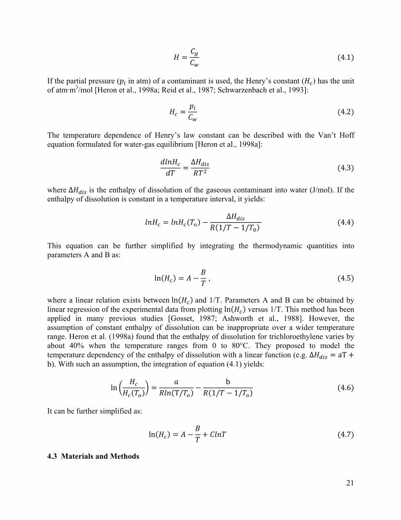
This equation can be further simplified by integrating the thermodynamic quantities into parameters A and B as:

ln , 4.5

where a linear relation exists between ln and 1/T. Parameters A and B can be obtained by linear regression of the experimental data from plotting ln versus 1/T. This method has been applied in many previous studies [Gosset, 1987; Ashworth et al., 1988]. However, the assumption of constant enthalpy of dissolution can be inappropriate over a wider temperature range. Heron et al. (1998a) found that the enthalpy of dissolution for trichloroethylene varies by about 40% when the temperature ranges from 0 to 80°C. They proposed to model the temperature dependency of the enthalpy of dissolution with a linear function (e.g. ∆ aTb). With such an assumption, the integration of equation (4.1) yields:

ln T/b

1/ 1/ 4.6

It can be further simplified as:

ln 4.7

4.3 Materials and Methods

21

Chemicals and Stock Solutions. The following chlorinated volatile organic compounds were selected for study: tetrachloroethylene (99%, ACROS ORGANICS), trichloroethylene (99.5%, Aldrich Chemical), chloroform (molecular biology certified, Shelton Scientific), 1,1,1-trichloroehane (Fisher scientific), 1,1-dichloroethane (TCI), dichloromethane (Burdick & Jackson), carbon tetrachloride (99.9%, Sigma-Aldrich), vinyl chloride (Matheson Gas Products), chloroethane (Sigma-Aldrich), chloromethane (Holox), cis-1,2-dichloroethylene (TCI), and 1,2-dichloroethane (Analytical agent, Mallinckrodt).

For analytical convenience, three mixtures of compounds were prepared. Mixture A contained methanol (0.900 g/g), tetrachloroethylene (0.0194 g/g), 1,1,1-trichloroethane (0.0156 g/g), trichloroethylene (0.0175 g/g), chloroform (0.0174 g/g), dichloromethane (0.0156, g/g), and 1,1-dichloroethane (0.0141, g/g). Mixture B contained methanol (0.963 g/g), carbon tetrachloride (0.0212 g/g) and 1,2-dichloroethane (0.0158 g/g). Mixture C contained methanol (0.982 g/g), chloromethane (3.65×10-4 g/g), vinyl chloride (3.54×10-4 g/g), chloroethane (2.86×10-4 g/g), and cis-1,2-dichloroethylene (0.0172 g/g).

EPICS Procedure. The original EPICS procedure was based on addition of equal amounts of volatile solute to two closed systems with different solvent volumes21. The gaseous concentrations of the two systems at equilibrium were measured and used to compute the dimensionless Henry’s law constant using the combined mass balance equations. However, this procedure has a low level of precision due to the constraint of delivering equal masses of solute to the systems [Lincoff and Gossett, 1984]. To improve on the precision, Gossett (1987) modified the EPICS procedure by using the mass ratio of added solute in the calculation of Henry’s law constant. This study follows the modified EPICS procedure. For each aqueous mixture at each temperature, six 160-mL serum bottles were used: three containing 100 mL distilled deionized (DDI) water, three containing 25 mL DDI water. Before the bottles were sealed with Teflon-lined red rubber septa and crimp caps, they were placed at the desired temperature for 5 minutes to equilibrate the pressure. Approximately 20 µL stock solution was then added to each sealed bottle. The exact amount of stock solution added was determined gravimetrically. For measurements at temperatures from 38°C to 93°C, the six EPICS serum bottles were submerged in a water bath at the desired temperatures for 3 hours. They were taken out and shaken every 15 minutes. For measurements at 21 °C, the bottles were placed on a shaker table overnight. For measurements at 8°C, the bottles were incubated for more than 24 hours in a water bath that was kept in a refrigerator.

Headspace Analysis of Volatile Compounds. Headspace concentrations at equilibrium were measured with a gas chromatograph (Hewlett Packard, 5890 Series II) equipped with a flame ionization detector, using the same temperature program described by Gossett (1987). The retention times of the studied chemicals ranged from 1.6 (chloromethane) to 14.5 min (tetrachloroethylene). Dimensionless Henry’s law constants were calculated with the following the equation:

/ / // / /

4.8

22

where and refer to the volumes of water and gas in serum bottles, M refers to the mass of solute added to the bottles, is the mass concentration of volatile compound in the gas phase, and subscripts 1 and 2 denote the serum bottles with different volumes of water. The calculation was repeated for every possible pair of bottles with differing volumes of water. The average and standard deviation were calculated based on the 9 values of H.

Measurement of Aqueous Solubility. Pure aqueous solubilities were measured for nine of the CVOCs using water-saturated solutions, as follows: For each chemical, a sufficient amount of neat liquid was added to a 160 mL serum bottle containing 150 mL of DDI water, such that a nonaqueous phase of the chemical was present. The serum bottles were sealed with Teflon-faced septa and incubated at the desired temperature for one week. The concentration of the CVOC in the aqueous phase was determined by removing less than 1 mL of the aqueous phase from each bottle and injecting it into a sealed serum bottle containing DDI water; the amount of DDI water was adjusted so that the total liquid volume present after adding the CVOC samples was 100 mL. Triplicate samples were taken for each compound. For analytical convenience, aqueous samples of different chemicals were mixed in the same combination used to measure Henry’s law constants (i.e., mixtures A, B, and C). These mixtures were placed on a shaker table at room temperature overnight before measuring the headspace concentrations by GC. Using externally prepared standards for each compound, the total amount of each compound present in the bottles was determined. This amount was divided by the volume of saturated water added to provide the saturation concentration.

4.4. Results and Discussion

Effect of Temperature on Henry’s Law Constant. Measured values and standard deviations for Henry’s constants at different temperatures are presented in Table 4.1. As expected, the Henry’s law constant is strongly dependent on temperature. For example, the Henry’s constant for tetrachloroethylene increases by a factor of around 24 from 8 to 91°C. Henry’s constants for trichloroethylene, chloroform, and 1,2-dichloroethane increase by 24-, 17-, and 30-fold from 8 to 93°C, respectively. Smaller variations were observed for 1,1,1-trichloroethane (8-fold), 1,1-dichloroethane (11-fold), dichloromethane (7-fold), carbon tetrachloride (9-fold), cis-1,2-dichloroethylene (13-fold), chloromethane (3-fold), chloroethane (6-fold), and vinyl chloride (10-fold).

The measured values of Henry’s law constants were compared with literature values. Generally, the measured values below 40 °C are close to the results reported by Gossett (1987) and the standard deviations of the data are of the same magnitude. The compound 1,2-dichloroethane was not included in the study by Gossett (1987). The measurement for 1,2-dichloroethane at 8°C has a high standard deviation. Values of Henry’s constant at other temperatures are close to the values reported by Ashworth et al. (1988). Görgényi et al. (2002) measured Henry’s law constants for chloroform, 1,1-dichloroethane, trichloroethylene, and several other chemicals using the EPICS-SPME technique (equilibrium partitioning in closed systems-solid phase microextraction) in the temperature range from 2 to 70°C. Our results for chloroform, 1,1-dichloroethane, and trichloroethylene in this temperature range are close to their reported values. Henry’s constants above 70°C are only available in the literature for trichloroethylene.

23

Table 4.1. Measured Henry’s Law Constants at Various Temperatures.

Compound Temperature (°C) H (dimensionless) Hc (m3·atm·mol-1) % SDa tetrachloroethylene 8.0 0.292 0.00673 3.24

24.0 0.676 0.01647 2.97 38.0 1.250 0.03190 3.26 58.0 2.293 0.06228 5.48 78.0 3.351 0.09653 18.4 90.0 3.701 0.11024 10.5 91.0 7.100 0.21207 29.1

trichloroethylene 8.0 0.165 0.00380 6.07 24.0 0.411 0.01002 3.96 38.0 0.675 0.01722 1.96 58.0 1.200 0.03260 4.20 78.0 1.705 0.04911 13.3 90.0 1.972 0.05875 7.39 91.0 2.784 0.08316 17.7 93.0 4.074 0.12235 36.1

chloroform 8.0 0.070 0.00160 47.8 24.0 0.145 0.00354 3.25 38.0 0.272 0.00694 6.34 58.0 0.466 0.01265 4.01 78.0 0.657 0.01892 10.0 90.0 0.794 0.02364 5.51 91.0 0.977 0.02920 12.1 93.0 1.192 0.03579 18.5

1,1,1-trichloroethane 8.0 0.304 0.00701 5.89 24.0 0.664 0.01619 2.38 38.0 1.093 0.02790 2.02 58.0 1.806 0.04905 5.37 78.0 2.063 0.05942 13.4 90.0 1.318 0.03925 17.9 91.0 1.203 0.03593 12.8 93.0 2.362 0.07095 30.5

1,1-dichloroethane 8.0 0.108 0.00249 17.1 24.0 0.226 0.00551 2.69 38.0 0.377 0.00962 3.69 58.0 0.603 0.01637 3.48 78.0 0.823 0.02370 10.1 90.0 0.949 0.02826 6.06 91.0 1.174 0.03507 13.1 93.0 1.506 0.04523 21.0

dichloromethane 8.0 0.081 0.00186 31.6 24.0 0.095 0.00230 23.6 38.0 0.159 0.00406 18.0 58.0 0.257 0.00697 5.49 78.0 0.350 0.01008 7.60

24

90.0 0.435 0.01296 5.96 91.0 0.504 0.01505 10.9 93.0 0.597 0.01792 13.7

carbon tetrachloride 8.0 0.493 0.01137 13.6 24.0 1.131 0.02756 2.81 38.0 2.018 0.05151 4.96 58.0 3.370 0.09154 11.9 78.0 4.972 0.14322 16.6 90.0 3.392 0.10105 20.1 93.0 4.585 0.13769 44.7

1,2-dichloroethane 8.0 0.010 0.00023 116.4 24.0 0.042 0.00103 18.8 38.0 0.097 0.00247 41.8 58.0 0.146 0.00397 6.85 78.0 0.228 0.00658 16.9 90.0 0.177 0.00529 15.1 93.0 0.299 0.00899 23.5

cis-1,2-dichloroethylene 8.0 0.077 0.00178 12.9 24.0 0.162 0.00396 4.28 38.0 0.299 0.00763 12.8 58.0 0.485 0.01318 9.69 78.0 0.694 0.01998 16.1 93.0 1.063 0.03191 23.1

chloromethane 8.0 0.315 0.00727 18.9 24.0 0.420 0.01023 4.82 38.0 0.577 0.01471 13.5 58.0 0.725 0.01969 3.80 78.0 1.133 0.03264 29.4 93.0 1.158 0.03477 15.9

chloroethane 8.0 0.253 0.00584 7.42 24.0 0.511 0.01246 7.06 38.0 0.739 0.01886 29.7 58.0 1.065 0.02892 7.76 78.0 1.178 0.03393 8.74 93.0 1.511 0.04539 25.3

vinyl chloride 8.0 0.589 0.01359 8.11 24.0 1.049 0.02557 3.60 38.0 1.404 0.03583 17.9 58.0 2.176 0.05911 4.14 78.0 2.153 0.06201 12.1 93.0 6.333 0.19019 60.6

a Percent standard deviation = 100(SD/mean).

25

Heron et al. (1998a) reported dimensionless Henry’s constants for trichloroethylene of 0.2, 0.4, 1.0, 1.2, 2.5, 3.7, and 4.6 at 10, 21, 50, 58, 81, 90, and 95°C, respectively. Similar results were obtained below 80°C in the present study. For measurements higher than 80°C, the values we obtained are about 30% lower than theirs. However, the standard deviations of measurements in this temperature range are larger than at ambient temperatures, with coefficients of variation (i.e., standard deviation/average) ranging from 7% to 36% in this study and about 30% or more in their study.

The modified EPICS method had good precision in the temperature range between 24 and 58°C. Except for a few compounds, coefficients of variation were within 10%. Increasing standard deviations were observed for measurements at temperatures higher than 78°C. Similar behavior was observed by Heron et al. (1998a). It appears that the EPICS method becomes less precise as the Henry’s law constant exceeds 3. Errors for measurements of chloroform (48%), dichloromethane (32%), and 1,2-dichloroethane (112%) were also relatively high at 8°C, perhaps due to the very low value of the Henry’s constants for these CVOCs at this temperature.

The temperature dependency of Henry’s law constants has been widely modeled with the Van’t Hoff equation [Heron et al., 1998a; Gosset, 1987; Ashworth et al., 1988]. Based on different assumptions used with respect to enthalpy of dissolution, equations (3) and (5) are used to empirically model Henry’s law constants [Heron et al., 1998a; Gosset, 1987; Ashworth et al., 1988]. The difference between equations (3) and (5) is that equation (3) assumes a constant enthalpy of dissolution [Gosset, 1987; Ashworth et al., 1988], while equation (5) assumes that the enthalpy is a linear function of temperature [Heron et al., 1998a]. Results from both linear and nonlinear regression of ln Hc versus 1/T are shown in Table 4.2 and Figure 4.1. From the r2 values and the graphs, it is apparent that equation (5) fits the data better.

Table 4.2. Temperature Regressions of Henry’s Law Constants.

Hc = exp(A-B/T + ClnT) Hc = exp(A-B/T) A B C r2 A B r2

tetrachloroethylene 152.2 10,547 -21.23 0.974 8.389 3,725 0.970trichloroethylene 98.26 7,936 -13.39 0.970 7.439 3,613 0.969chloroform 136.4 9,647 -19.23 0.990 5.920 3,438 0.9861,1,1-trichloroethane 537.7 27,579 -78.84 0.919 2.985 2,128 0.7901,1-dichloroethane 132.7 8,917 -18.96 0.980 4.091 2,795 0.975dichloromethane -114.7 -2,908 17.39 0.987 3.201 2,706 0.982carbon tetrachloride 460.6 24,398 -67.08 0.983 5.834 2,813 0.916 1,2-dichloroethane 659.0 34,827 -96.36 0.980 5.766 3,821 0.906 cis-1,2-dichloroethylene 161.6 10,739 -23.01 0.996 5.806 3,375 0.989 chloromethane 13.35 2,509 -1.661 0.990 2.103 1,977 0.989 chloroethane 252.6 14,112 -36.79 0.992 3.382 2,337 0.959 vinyl chloride -132.4 -3775 20.36 0.925 5.469 2,741 0.918

26

Tetrachloroethylene

T (K)280 300 320 340 360

lnH

c

-5

-4

-3

-2 MeasuredlnHc=A-B/T+ClnTlnHc=A-B/T

Trichloroethylene

T (K)280 300 320 340 360

lnH

c

-6

-5

-4

-3

-2MeasuredlnHc=A-B/T+ClnT lnHc=A-B/T

1,1-Dichloroethane

T (K)280 300 320 340 360

lnH

c

-6.0

-5.5

-5.0

-4.5

-4.0

-3.5MeasuredlnHc=A-B/T+ClnTlnHc=A-B/T

Chloroform

T (K)280 300 320 340 360

lnH

c

-7

-6

-5

-4

-3

MeasuredlnHc=A-B/T+ClnTlnHc=A-B/T

1,1,1-Trichloroethane

T (K)280 300 320 340 360

lnH

c

-5.0

-4.5

-4.0

-3.5

-3.0

-2.5

MeasuredlnHc=A-B/T+ClnTlnHc=A-B/T

Dichloromethane

T (K)280 300 320 340 360

lnH

c

-6.5

-6.0

-5.5

-5.0

-4.5 Measured lnHc=A-B/T+ClnTlnHc=A-B/T

27

Carbon Tetrachloride

T (K)280 300 320 340 360

lnH

c

-4.5

-4.0

-3.5

-3.0

-2.5

-2.0

MeasuredlnHc=A-B/T+ClnTlnHc=A-B/T

1,2-Dichloroethane

T (K)280 300 320 340 360

lnH

c

-8

-7

-6

-5

MeasuredlnHc=A-B/T+ClnTlnHc=A-B/T

cis-1,2-Dichloroethylene

T (K)280 300 320 340 360

lnH

c

-6.5

-6.0

-5.5

-5.0

-4.5

-4.0

-3.5Measured lnHc=A-B/T+ClnTlnHc=A-B/T

Chloromethane

T (K)280 300 320 340 360

lnH

c

-5.0-4.8-4.6-4.4-4.2-4.0-3.8-3.6-3.4-3.2

Measured lnHc=A-B/T+ClnTlnHc=A-B/T

Chloroethane

T (K)280 300 320 340 360

lnH

c

-5.0

-4.5

-4.0

-3.5

-3.0MeasuredlnHc=A-B/T+ClnTlnHc=A-B/T

Vinyl Chloride

T (K)280 300 320 340 360

lnH

c

-4.5

-4.0

-3.5

-3.0

-2.5

-2.0

-1.5

MeasuredlnHc=A-B/T+ClnTlnHc=A-B/T

Figure 4.1. Temperature regression of Henry’s law constants.

28

Table 4.3. Aqueous Solubilities of Chlorinated Volatile Compounds. Compound Temperature (°C) Solubility (mg/L) % SD tetrachloroethylene 8 209 6.51

21 197 8.64 35 236 2.34 60 256 3.40 75 320 2.37

trichloroethylene 8 1,223 5.201 21 1,338 2.68 35 1,310 0.79 60 1,384 1.88 75 1,503 0.89

1,1,1-trichloroethane 8 1,354 10.7 21 1,059 2.74 35 1,313 0.84 60 1,008 2.82 75 719 0.10

chloroform 8 8,424 3.24 21 8,416 3.13 35 7,422 1.54 60 7,454 2.78 75 7,902 2.41

1,1-dichloroethane 8 5,403 0.40 21 5,490 2.65 35 5,265 2.92 60 5,434 3.47 75 5,471 3.85

dichloromethane 8 9,760 8.14 21 - - 35 18,842 3.44 60 19,391 2.84 75 - -

carbon tetrachloride 8 871 0.90 21 559 7.08 35 765 2.00 60 839 1.10 75 849 2.29

1,2-dichloroethane 8 8,073 5.14 21 8,912 0.40 35 8,975 0.12 60 9,679 0.27 75 10,305 0.13

cis-1,2-dichloroethylene 8 6,954 3.71 21 7,026 1.99 35 7,044 3.36 60 6,937 2.19 75 7,178 0.82

29

The overall slopes obtained in this study were compared with previous findings based on measurements at low temperatures. The slopes obtained in this study using linear regression (equation 3) are about one-third to two-thirds lower than those of Gossett 2. This supports the conclusion from Heron et al. (1998a) that it is not appropriate to extrapolate the data from measurements at low temperature by assuming that the enthalpy of dissolution is constant.

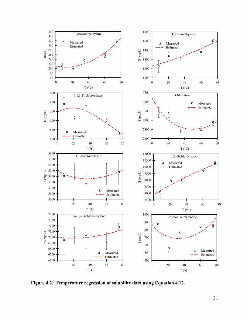
Effect of Temperature on Aqueous Solubility. The aqueous solubilities of tetrachloroethylene, trichloroethylene, chloroform, 1,1,1-trichloroethane, 1,1-dichloroethane, dichloromethane, carbon tetrachloride, 1,2-dichloroethane, and cis-1,2-dichloroethylene were measured between 8 and 75°C. The measured values are presented in Table 4.3 and Figure 4.2. Except for tetrachloroethylene at 21°C, the coefficients of error at temperatures above 20°C are within 4%. Coefficients of error at 8°C range from 0.90% to 10.7%. Different chemicals showed different patterns of temperature dependence of solubility. For trichloroethylene, solubility increased from 1223 mg/L at 8 °C to 1503 mg/L at 75°C. Similar patterns was seen for tetrachloroethylene and 1,2-dichloroethane. The solubility of 1,1,1-trichloroethane fluctuated in the range of 1008-1354 mg/L at temperatures from 8 to 60°C and decreased to 719 mg/L at 75°C. The solubility of chloroform decreased from 8424 mg/L at 8°C to 7422 mg/L at 35°C, and increased to 7902 at 75°C. The solubility of cis-1,2-dichloroethylene and 1,1-dichloroethane changed little with temperature.

Heron et al. (1998a) measured the solubility of trichloroethylene between 9 and 71°C using a column generator technique. Their measured values range between 1300 mg/L and 1500 mg/L, with a minimum value around 30°C. This is close to what we measured. Knauss et al. (2000) reported solubilities for trichloroethylene in the range of 1417 mg/L (21°C) to 1878 mg/L (75°C) and for tetrachloroethylene in the range of 200 mg/L at 21°C to around 300 mg/L at 75°C. The solubilities of trichloroethylene measured in this study are lower than their results, but the results for tetrachloroethylene are close.

Vapor Pressure-Solubility Model. One predictive method for estimating Henry’s constants at high temperature is to divide the vapor pressure by the aqueous solubility [Mackay and Shiu, 1991; Brennan et al., 1998].

where is Henry’s law constant in atm·m3/mol, is pure vapor pressure in atm, and is aqueous solubility in mol/m3.

4.9

The values of pure vapor pressure were calculated with the Frost-Kalkwarf-Thodos equation [Reid et al., 1987] for 1,1-dichloroethane

4.10

30

Tetrachloroethylene

T (°C)0 20 40 60 80

S (m

g/L)

160180200220240260280300320340360

MeasuredEstimated

Trichloroethylene

T (°C)0 20 40 60 80

S (m

g/L)

1100

1200

1300

1400

1500

1600

MeasuredEstimated

1,1,1-Trichloroethane

T (°C)0 20 40 60 80

S (m

g/L)

600

800

1000

1200

1400

1600

MeasuredEstimated

Chloroform

T (°C)0 20 40 60 80

S (m

g/L)

7000

7500

8000

8500

9000

9500

MeasuredEstimated

1,1-Dichloroethane

T (°C)0 20 40 60 80

S (m

g/L)

5000

5100

5200

5300

5400

5500

5600

5700

5800

MeasuredEstimated

1,2-Dichloroethane

T (°C)0 20 40 60 80

S (m

g/L)

7500

8000

8500

9000

9500

10000

10500

11000

MeasuredEstimated

cis-1,2-Dichloroethylene

T (°C)0 20 40 60 80

S (m

g/L)

6600

6700

6800

6900

7000

7100

7200

7300

7400

MeasuredEstimated

Carbon Tetrachloride

T (°C)0 20 40 60 80

S (m

g/L)

400

500

600

700

800

900

1000

MeasuredEstimated

31

Figure 4.2. Temperature regression of solubility data using Equation 4.12.

Figure 4.3. Prediction of Henry’s Law constant with the ratio of vapor pressure to solubility using Equation 4.9.

32

and Wagner equation [Reid et al., 1987] for the rest of compounds

ln 1 . , 4.11

where 1 / , is absolute temperature (K), is critical temperature (K), is vapor pressure (bar), is critical pressure (bar), , , , and are constants specific for each pure compound. These values were obtained from Reid et al. (1987).

Regression of the aqueous solubility data as a function of temperature was conducted with the following equation [Knauss et al., 2000]:

4.12

where the K is the solubility in mole fraction, T is absolute temperature in Kelvin, R is the universal gas constant, and D, E and F are curve fitting parameters. The values of these parameters as well as the r2 values are shown in Table 4; the model fit to the data are shown in Figure 2 (except for dichloromethane). The calculated value of solubility using this equation as a function of temperature is further used for the calculation of Henry’s law constant, as shown in Figure 3. Overall, there is good agreement between the estimated and measured Henry’s law constants. For temperatures higher than 75°C, the predicted values are sometimes higher than the measured values. A possible reason for this is the underestimation of the aqueous solubility of the compounds at these higher temperatures. Knauss et al. (2000) measured the aqueous solubilities of TCE and PCE over a wider range of temperature (21-161°C). They found that the solubility of TCE and PCE increases at a higher rate at higher temperatures.

Table 4.4. Temperature Regression of Aqueous Solubility.

D E F r2 1,2-dichloroethane -6.76571 -4,417 -5.60996 0.952 tetrachloroethylene -1313.04 52,334 184.0563 0.932 trichloroethylene -220.293 5,136 23.03885 0.862 chloroform -835.754 37,099 115.0121 0.717 1,1,1-trichloroethane 1863.286 -84,438 -289.987 0.790 carbon tetrachloride -2039.44 89,308 291.6319 0.344 cis-1,2-dichloroethylene -125.696 3,082 10.54612 0.339 1,1-dichloroethane -241.997 8,465 27.37585 0.283

33

The results of this study indicate a strong effect of temperature on Henry’s law constants, which increased from 3-fold (chloroethane) to 30-fold as temperature increased from 8 to 93°C. Because the enthalpy of dissolution is a function of temperature, it is not appropriate to extrapolate the Henry’s law constant from measurements at low temperature using a linear function. The nonlinear function proposed by Heron et al. (1998a) that incorporates a temperature dependent enthalpy provides a better fit to the experimental data. Using measured data for solubility, the vapor pressure-solubility model gives a reasonable prediction of the Henry’s law constants. With improved data on Henry’s law constants at high temperatures for 12 common CVOC measured in this study, it will be possible to more accurately model subsurface remediation processes that operate near the boiling point of water.

4.5. References

Abraham, M. H.; Jr., W. E. A., Prediction of gas to water partition coefficients from 273 to 373 K using predicted enthalpies and heat capacities of hydration. Fluid Phase Equilibria 2007, 262, 97-110.

Ashworth, R. A.; Howe, G. B.; Mullins, M. E.; Rogers, T. N., Air-water partitioning coefficients of organics in dilute aqueous solutions. Journal of Hazardous Materials 1988, 18, 25-36.

Beyke, G.; Fleming, D., In situ thermal remediation of DNAPL and LNAPL using electrical resistance heating. Remediation 2005, 15, (3), 5-22.

Brennan, R. A.; Nirmalakhandan, N.; Speece, R. E., Comparison of predictive methods for Henry's law coefficients of organic chemicals. Water Research 1998, 32, (6), 1901-1911.

Chen, F.; Liu, X.; Falta, R. W.; Murdoch, L. C., Experimental demonstration of contaminant removal from fractured rock by boiling. Environmental Science & Technology 2010, 44, 6437-6442.

Heron, G.; Christensen, T. H.; Enfield, C. G., Henry's law constant for trichloroethylene between 10 and 95 °C. Environmental Science & Technology 1998a, 32, (10), 1433-1437.

Heron, G.; Parker, K.; Galligan, J.; Holmes, T. C., Thermal treatment of eight CVOC source zones to near nondetect concentrations. Ground Water Monitoring & Remediation 2009, 29, (3), 56-65.

Hodges, R. A.; Falta, R.; Stewart, L., Controlling steam flood migration using air injection wells. Environmental Geosciences 2004, 11, (4), 221-238.

Gauglitz, P.; Roberts, J.; Bergsman, T.; Schalla, R.; Caley, S.; Schlender, M.; Heath, W.; Jarosch, T.; Miller, M.; Eddy-Dilek, C.; Moss, R.; Looney, B. Six-phase soil heating for enhanced removal of contaminants: Volatile organic compounds in nonarid soils. Integrated demonstration, Savannah River Site; Richland, CA, 1994.

34

Görgényi, M.; Dewulf, J.; Langenhove, H. V., Temperature dependence of Henry's law constant in an extended temperature range. Chemosphere 2002, 48, 757-762.

Gossett, J. M., Measurement of Henry's law constants for C1 and C2 chlorinated hydrocarbons. Environmental Science and Technology 1987, 21, 202-208.

Gudbjerg, J.; Sonnenborg, T. O.; Jensen, K. H., Remediation of NAPL below the water table by steam-induced heat conduction. Journal of Contaminant Hydrology 2004, 72, 207-225.

Heron, G.; Christensen, T. H.; Zutphen, M. V.; Enfield, C. G., Soil heating for remediation of dissolved trichloroethylene in low-permeable soil. Battelle Press: Columbus, Ohio, 1998b.

Knauss, K. G.; Dibley, M. J.; Leif, R. N.; Mew, D. A.; Aines, R. D., The aqueous solubility of trichloroethene (TCE) and tetrachloroethene (PCE) as a function of temperature. Applied Geochemistry 2000, 15, 501-512.

Lau, K.; Rogers, T. N.; Zei, D. A., Modeling the temperature dependence of the Henry's law constant of organic solutes in water. Fluid Phase Equilibria 2010, 290, 166-180.

Lincoff, A. H.; Gossett, J. M., The determination of Henry's law constant for volatile organics by equilibrium partitioning in closed systems. Reidel: Boston, 1984.

Mackay, D.; Shiu, D., A critical review of Henry's law constants for chemicals of environmental interest. Journal of physical and chemical reference data 1991, 10, 1175-1202.

Ochs, S. O.; Hodges, R. A.; Falta, R. W.; Kmetz, T. F.; Kupar, J. J.; Brown, N. N.; Parkinson, D. L., Predicted heating patterns during steam flooding of coastal plain sediments at the Savannah River Site. Environmental and Engineering Geoscience 2003, 9, (1), 51-69.

Plyasunov, A. V.; Shock, E. L., Prediction of the vapor-liquid distribution constants for volatile nonelectrolytes in water up to its critical temperature. Geochimica et Cosmochimica Acta 2003, 67, (24), 4981-5009.

Reid, R. C.; Prausnitz, J. M.; Poling, B. E., The properties of gas & liquids. fourth edition ed.; McGraw-Hill Book Company: 1987.

Schwarzenbach, R. P.; Gschwend, P. M.; Imboden, D. M., Environmental organic chemistry. John Wiley & Sons, Inc: New York, 1993.

Staudinger, J.; Roberts, P. V., A critical compilation of Henry's law constant temperature dependence relations for organic compounds in dilute aqueous solutions. Chemosphere 2001, 44, 561-576.

35

5. Numerical Analysis of Contaminant Removal From Fractured Rock by Boiling (to be submitted to the Journal of Contaminant Hydrology, 2011)

5.1 Introduction

Contaminant removal from fractured rock by boiling has recently been demonstrated in a laboratory experiment (Chen et al. 2010). After boiling away about 1/3 of the pore volume of water from a contaminated sandstone core, approximately 100% recovery of 1,2-dichloroethane (1,2-DCA) was achieved (Chen et al. 2010). However, the phenomenon of contaminant mass transfer from fractured geologic media during boiling is complex due to the strong coupling among the heat transfer, multiphase flow, and thermodynamics. To investigate such a phenomenon, numerical simulation is helpful to better understand the coupled mass and heat transfer during the boiling process.

The T2VOC and TMVOC codes have been widely used for simulation of multiphase flow with single and multiple volatile organic chemical(s) (Falta et al. 1995,Pruess and Battistelli. 2003,Tse et al. 2006). They were validated with experimental results for a variety of isothermal and non-isothermal problems (Adenekan. 1992,Adenekan et al. 1993,Falta et al. 1992b,Gudbjerg et al. 2004,Ochs et al. 2003). However, contaminant mass transfer between matrix blocks and fractures due to boiling has not received much attention to date, and it is helpful to establish the reliability of the codes in predicting such experimental results.

In this paper, the TMVOC code is used to simulate a laboratory experiment for contaminant removal from fractured rock by boiling. Next, the 1-D contaminant mass removal from the fractured rock by boiling is numerically analyzed without experimental end effects. Finally, simulation of field-scale application of thermal remediation is conducted, using a special discretization that can resolve local fracture-matrix interactions.

5.2. TMVOC simulator

For a multiphase system the governing equations consist of several mass balance and an energy balance equations that sum over the fluid and rock phases. The mass components can be H2O, multiple volatile organic compounds (VOC), and noncondensible gas. In this study, the components are H2O, 1,2-DCA, NaBr, and air. The TMVOC codes are capable of modeling 3-phase flow of NAPL, liquid water, and gas using multiphase extension of Darcy’s law. Since dissolved 1,2-DCA was used in the experiment and no NAPL phase was involved, two-phase flow (gas and liquid water) is considered here in the model. The multiphase Darcy’s law includes relative permeability effects, which are calculated using standard 2-phase functions of the phase saturations (van Genuchten. 1980,Verma. 1986). The fluid flow is driven by the phase pressure gradient with capillary pressure, and a gravity term depending on the phase density. Capillary pressure is computed as a function of phase saturation using various functions (van Genuchten. 1980). The transport of mass components in each fluid phase considers advection, and diffusion including temperature and pressure dependent diffusion coefficients, and phase saturation dependent tortuosities. Linear equilibrium adsorption to the rock or soil is taken into account for the contaminant component. Heat transfer considers multiphase convection including both latent and sensible heat, and thermal conduction. The thermal conductivity is treated as a nonlinear

36

function of liquid saturation. Both thermal and flow properties of the rock or soil can be heterogeneous.

The thermodynamic properties of water were built into the codes, and the thermodynamic properties of CVOC are calculated using the corresponding states method (Falta et al. 1995, Falta et al. 1992a, Pruess and Battistelli. 2002). The treatment of the heat transfer and thermodynamics allows for rigorous consideration of boiling and condensation of multicomponent mixtures, including noncondensible gas effects. The nonlinear coupled mass and energy balance equations are linearized using an implicit residual-based Newton-Raphson iterative technique, and solved using a selection of direct and iterative matrix solvers (Pruess and Battistelli. 2002).

5.3. Simulation of the experiment

Heating Experiment. A laboratory study has been conducted on the demonstration of CVOC removal from fractured rock by boiling (Chen et al. 2010). The experimental system used in the study is as shown in Figure . An unfractured Berea sandstone core was used to represent the material while the end to represent the fracture. The core has an intrinsic permeability of 1.5×10-

13 m2 and a porosity of 0.174. It was sealed with Teflon shrink tube and Aluminum end-caps, and wrapped with a strip heater and an insulation layer. A set of cartridge heaters was placed in each Teflon plate to counteract the heat loss at ends. The core assembly was hung in a pressurized vessel to keep the Teflon tube in contact with the core. The effluent from the core was routed to a condenser, and the generated steam was condensed before it was collected in partially vacuumed sealed vials. Headspace samples were analyzed in Gas Chromatography and liquid samples were analyzed in Ion Chromatography (Chen et al. 2010).

Figure 5.1 Diagram of experimental setup (Chen et al. 2010).

37

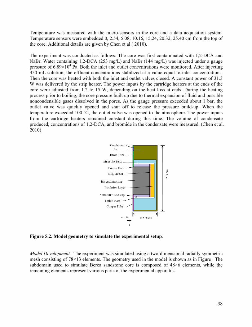
Temperature was measured with the micro-sensors in the core and a data acquisition system. Temperature sensors were embedded 0, 2.54, 5.08, 10.16, 15.24, 20.32, 25.40 cm from the top of the core. Additional details are given by Chen et al ( 2010).

The experiment was conducted as follows. The core was first contaminated with 1,2-DCA and NaBr. Water containing 1,2-DCA (253 mg/L) and NaBr (144 mg/L) was injected under a gauge pressure of 6.89×104 Pa. Both the inlet and outlet concentrations were monitored. After injecting 350 mL solution, the effluent concentrations stabilized at a value equal to inlet concentrations. Then the core was heated with both the inlet and outlet valves closed. A constant power of 31.3 W was delivered by the strip heater. The power inputs by the cartridge heaters at the ends of the core were adjusted from 1.2 to 15 W, depending on the heat loss at ends. During the heating process prior to boiling, the core pressure built up due to thermal expansion of fluid and possible noncondensible gases dissolved in the pores. As the gauge pressure exceeded about 1 bar, the outlet valve was quickly opened and shut off to release the pressure build-up. When the temperature exceeded 100 °C, the outlet valve was opened to the atmosphere. The power inputs from the cartridge heaters remained constant during this time. The volume of condensate produced, concentrations of 1,2-DCA, and bromide in the condensate were measured. (Chen et al. 2010)

Figure 5.2. Model geometry to simulate the experimental setup.

Model Development. The experiment was simulated using a two-dimensional radially symmetric mesh consisting of 78×13 elements. The geometry used in the model is shown as in Figure . The subdomain used to simulate Berea sandstone core is composed of 48×6 elements, while the remaining elements represent various parts of the experimental apparatus.

38

Table 5.1 Values of material properties used in the simulation.

Subdomain Porosity Permeability (m2)

Density (kg/m3)

Thermal conductivity (W/m°C)

Specific heat (J/kg°C)

Berea Sandstone

0.167 1.5×10-13 2491 3.57 (wet) 1.75 (dry)

1680

Heater 0.001 1.0×10-18 501.2 1.07 1029 Porous Disk 0.16 1.0×10-10 3950.0 41.22 1356.5 Aluminum End-Cap

0.001 1.0×10-18 2702 237 903

Outlet Tube 0.0559 1.46×10-10 8730 60 427 Condenser 0.0559 1.46×10-10 1.0×1010 60 10001.0 Inlet Tube 0.14 3.15×10-10 8940 400 427.8 Teflon Plate 0.001 1.0×10-18 2200 0.5 1001.0 Insulation Layer

0.01 1.0×10-18 100 0.28 844.0

Air in the vessel

0.99 1.0×10-18 1.09×105 0.2 1009.0

Air out of the vessel

0.99 1.0×10-18 1.2×1010 0.2 10001.0

The values of material properties are shown in Table 5.1. Properties for the core are assigned with the experimentally determined values. A small porosity (0.001) and an extremely low permeability (1.0×10-18 m2) are used for the heater and Aluminum cap in the model to simulate the sealed condition of the core (no fluid flow from the core through heater or aluminum cap). Typical values of the materials are used for the density, thermal conductivity, and specific heat. During the heating experiment, the air temperature increased to 36 C in the vessel. Thus, a high value (1.09×105 kg/m3) is given to the air density of the air in the vessel to simulate the temperature increase during the heating experiment. Constant temperature boundary is applied to the air out of the vessel and condenser subdomains by assigning extremely high values of density and specific heat. The density and specific heat for the air out of the vessel are assigned with 10001.0 J/kg°C and 1.2×1010 kg/m3, respectively. The condenser was assigned with a density of 1×1010 kg/m3 and a specific heat of 10001.0 J/kg°C to maintain the temperature at constant 5 °C.

Thermal Conductivity and Specific Heat. The thermal conductivity and specific heat of the rock sample were measured using the dual-probe heat-pulse method. This in-situ transient method has been used in the determination of thermal properties of soil and rock samples in many previous literatures (Bachmann et al. 2001,Bristow et al. 1994,Carslaw and Jaeger. 1959,de Vries. 1952,Kluitenberg et al. 1993,Knight et al. 2007,Kubičár et al. 2006,Lewis et al. 1993,Lu et al. 2007,Muñoz et al. 2009,Tarara and Ham. 1997,Welch et al. 1996). This in-situ transient method was developed based on the analytical solution for temperature distribution around an instantaneously heated infinite line source. It was described by Carslaw and Jaeger (1959) as:

39

, (5.1)

where is temperature (°C), is radial distance from the line source (m), is time (s), is the thermal diffusivity (m2/s) of the medium surrounding the heater, is the finite quantity of heat liberated by the line source, which is calculated with:

(5.2)

Here, is the quantity of the heat liberated per unit length of heater, is the volumetric heat capacity of the medium.

The thermal diffusivity and volumetric capacity are obtained by taking the derivative of the equation (5.1) in terms of time. At the peak of the temperature profile ( ), the first derivative of equation (5.1) is equal to zero. The thermal diffusivity and volumetric capacity are expressed as (Bristow et al. 1994,Campbell et a 91,l. 19 Jaeger. 1965,Lubimova et al. 1961):

(5.3)

and

∆ (5.4)

where e is the natural exponent, ∆ is maximum temperature change.

Considering the duration of the heat pulse ( ), thermal diffusivity can be calculated with the following modified equation (Bristow et al. 1994,Lubimova et al. 1961):

(5.5)

Knowing the thermal diffusivity and volumetric capacity, one can calculate the thermal conductivity by multiplying the thermal usivity and vo diff lumetric heat capacity:

(5.6)

The measurement was conducted as follows: a rock sample (7.62 cm long, 5.08 cm in diameter) was cut from the sandstone core used in the experiment. Two parallel holes (6mm apart, 2.54 cm deep) were drilled in the core, embedded with a microheater and a thermistor. The microheater consists of a stainless steel tube (3.575 cm, O.D.) and a 10-cm-long enameraled Evanohm wire (Pelican Wire Co., Naples, FL), twice doubly folded in the tube. The thermistor was connected to a data acquisition system for temperature measurement.

40

As shown in Figure , the microheater was connected to a 9V power supply (HQ Power, Fort Worth, TX) through a transistor board and a 10 Ω resistor. The transistor board functions as a switch, turning on and off the microheater, according to the digital signals from an I/O unit (NI-6008) that is controlled by a Labview program. A heat pulse was generated by turning on the microheater for 10 seconds and shutting off, while the temperature was monitored every second.

Figure 5.3 Experimental setup for thermal property measurement.

This dual-probe heat-pulse method was calibrated with gelled water. It was prepared as follows: 1% (w/w) agar powder (Becton, Dickinson, MD) was mixed in water at temperature close to 100 C. Cooling down to about 70 °C, the mixture was poured to a cylindrical container that has inner diameter of 5.08 cm. After aging for hours, the cylindrical gel was ready for thermal property measurement (Zhu et al. 2007). Due to the high percentage of liquid water, this immobile water has almost the same thermal conductivity of liquid water. Moreover, it eliminates the possible measurement error caused by heat transfer by convection. The thermal conductivity and specific heat of water is well known. Thus the measured values of gelled water can be used for calibration of the dual-probe method.

The measured thermal conductivities of the Berea sandstone core at both wet and dry conditions are 3.57 W/m K and 1.75 W/m K, respectively. The partially saturated porous media thermal conductivity λ is computed in the model using a nonlinear variation (Pruess and Battistelli. 2002)

(5.7)

where is the dry porous media thermal conductivity, is the water-saturated porous media thermal conductivity. The measured specific heat is 1680 J/kg°C.

Relative Permeability and Capillary Pressure. The capillary pressure and relative permeability curves used in the simulation are summarized in Table 5.2. The data of air relative permeability and capillary pressure as functions of water saturation were collected from two pieces of 3-inch core cut from the core used in the experiment. Measurements were conducted by Daniel B. Stephens & Associates, Inc.

41

The gas-water capillary pressures at different water saturation were fit with the van Genuchten equation (Parker et al. 1987,van Genuchten. 1980).

/1

/ (5.8)

where m=1-1/n, Swr is the residual water saturation, αgn, αnw,and n are curve shape parameters. They are adjusted to fit the experimental data (see Figure ), yielding αnw=αgn=2.22, n=1.56 and Swr =0.051, respectively.

The function used to model the gas relative permeability at different saturation was modified from the one used by Verma ( 98 -liquid system 1 6) for steam s:

(5.9)

with

..

(5.10)

where is water saturation, is residual water saturation, is the maximum water saturation. This equation was developed for the steam-water relative permeability and has a good fit with the experimental measurements (Verma and Pruess. 1986,Verma. 1986). Parameters A, B, C and D are adjusted to fit the data from the experiment (A=0.931, B=-2.87, C=2.59, D=-0.651). The relative permeability curves are shown in Figure .

Water saturation0.0 0.2 0.4 0.6 0.8 1.0

Pres

sure

hea

d (c

m)

1e+1

1e+2

1e+3

1e+4

1e+5

1e+6

FitMeasured

Figure 5.4 Capillary pressure curve of the Berea sandstone core

42

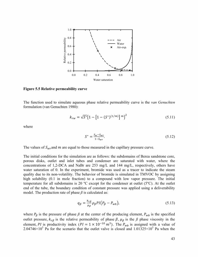
Water saturation0.0 0.2 0.4 0.6 0.8 1.0

Rel

ativ

e pe

rmea

bilit

y

0.0

0.2

0.4

0.6

0.8

1.0

AirWaterAir-exp.

Figure 5.5 Relative permeability curve

The function used to simulate aqueous phase relative permeability curve is the van Genuchten formulation (van Genuchten 1 80)9 :

√ 1 1 ⁄ (5.11)

where

. (5.12)

The values of and are equal to those measured in the capillary pressure curve.

The initial conditions for the simulation are as follows: the subdomains of Berea sandstone core, porous disks, outlet and inlet tubes and condenser are saturated with water, where the concentrations of 1,2-DCA and NaBr are 253 mg/L and 144 mg/L, respectively, others have water saturation of 0. In the experiment, bromide was used as a tracer to indicate the steam quality due to its non-volatility. The behavior of bromide is simulated in TMVOC by assigning high solubility (0.1 in mole fraction) to a compound with low vapor pressure. The initial temperature for all subdomains is 20 °C except for the condenser at outlet (5°C). At the outlet end of the tube, the boundary condition of constant pressure was applied using a deliverability model. The production rate of phase ß is calculated as:

, (5.13)

where is the pressure of phase ß at the center of the producing element, is the specified outlet pressure, is the relative permeability of phase , is the ß phase viscosity in the element, is productivity index ( 1 10 . The is assigned with a value of 2.04746×105 Pa for the scenario that the outlet valve is closed and 1.01325×105 Pa when the

43

outlet valve is open to the atmosphere. When the pressure at the center of the producing element is higher than the specified outlet pressure, the production rate is calculated as equation 13. When it is less than the specified outlet pressure, the production rate is zero. The condenser is simulated by assigning a high specific heat to maintain a constant temperature.

Henry’s Law Constant of 1,2-DCA . Henry’s law constant is important in determining the partitioning of a volatile organic compound from aqueous to gaseous phases. The values for chlorinated solvents are strongly dependent on temperature (Chen et al.,Heron et al. 1998a). To better simulate the process of CVOC partitioning at elevated temperatures, it is necessary to include the temperature dependency of Henry’s law constant in the model.

The Henry’s law constant of 1,2-DCA at temperatures from 8 to 93°C (shown in Figure ) were measured using modified Equilibrium Partitioning In Closed Systems (EPICS) procedure (Chen et al.,Gossett. 1987,Heron et al. 1998a). In this method, six 160-mL serum bottles were used at each temperature: three containing 100 mL distilled deionized (DDI) water and three containing 25 mL DDI water. These bottles were placed at the desired temperature for 5 minutes to equilibrate the pressure before they were sealed with Teflon-lined rubber septa and crimp caps. A mixture that contained methanol (0.963 g/g), carbon tetrachloride (0.0212 g/g) and 1,2-dichloroethane (0.0158 g/g) was prepared as a stock solution. Approximately 20 µL stock solution was then added to each sealed bottle and the exact amount added was determined gravimetrically. The equilibration at different temperatures was conducted as follows: for measurements at temperatures from 38°C to 93°C, the bottles were submerged in a water bath at the desired temperatures for 3 hours. They were taken out and shaken every 15 minutes. For the measurements at 21°C, the bottles were placed on a shaker table overnight. For the measurements at 8°C, the bottles were incubated for more than 24 hours in a water bath that was kept in a refrigerator.

Headspace concentration of 1,2-DCA at equilibrium was measured with a gas chromatograph (Hewlett Packard, 5890 Series II) equipped with a flame ionization detector. The temperature program used in this measurement was the same as described by Gossett ( 1987). The dimensionless Henry’s law constant of 1,2-DCA was calculated with (Gossett. 1987):

/ / // / /

(5.14)

where and denote the volumes of water and gas in serum bottles, M represent the mass of 1,2-DCA added to the bottles, is the mass concentration of 1,2-DCA in the gas phase, and subscripts 1 and 2 stand for the serum bottles with different volumes of water. The was calculated for every possible pair (9 pairs) of bottles with differing volumes of water, based on which the average and standard deviation were obtained. The results are shown in Figure .

The temperature dependence of Henry’s law constant of 1,2-DCA is simulated using

(5.15)

44

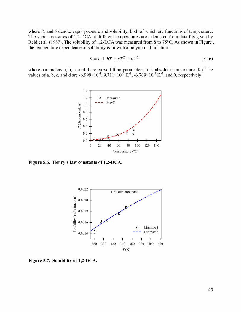
where and denote vapor pressure and solubility, both of which are functions of temperature. The vapor pressures of 1,2-DCA at different temperatures are calculated from data fits given by Reid et al. (1987). The solubility of 1,2-DCA was measured from 8 to 75°C. As shown in Figure , the temperature dependence of solubility is fit with a polynomial function:

(5.16)

where parameters a, b, c, and d are curve fitting parameters, T is absolute temperature (K). The values of a, b, c, and d are -6.999×10-4, 9.711×10-6 K-1, -6.769×10-9 K-2, and 0, respectively.

Temperature (°C)0 20 40 60 80 100 120 140

H (d

imen

sion

less

)

0.0

0.2

0.4

0.6

0.8

1.0

1.2

1.4

MeasuredPvp/S

Figure 5.6. Henry’s law constants of 1,2-DCA.

1,2-Dichloroethane

T (K)280 300 320 340 360 380 400 420

Solu

bilit

y (m

ole

frac

tion)

0.0014

0.0016

0.0018

0.0020

0.0022

Measured Estimated

Figure 5.7. Solubility of 1,2-DCA.

45

Simulation Results The simulated temperature profile is compared with the experimentally determined profile in Figure . Before boiling occurs, the simulated temperatures at all locations were in a good agreement with the experimentally determined temperatures. After the outlet valve was open to the atmosphere (2.73 hours), the simulated core temperature at the outlet (T1_Sim) was similar to the experimentally determined one (T1_Exp), dropping the temperature to close to 100°C immediately. However, the simulated temperatures (T2_Sim-T7_Sim) at deeper locations were somewhat higher than the temperatures measured in the experiment (T2_Exp-T7_Sim). Therefore, compared to the experiment, a higher temperature gradient was observed in the simulated results.

This overestimated temperature gradient is possibly due to the fact that the steam-water relative permeability curve used in the model was fit to air permeability data. It has been repeatedly noted that steam-water relative permeability is different from the air-water relative permeability (Horne et al. 2000,Li and Horne. 2004,Verma and Pruess. 1986,Verma. 1986). Verma (1986) measured the steam relative permeability and found the enhanced steam permeability due to phase transition effects (Verma and Pruess. 1986,Verma. 1986). The phase transition along the interface of a stagnant phase and the phase flowing around it results in a reduction in irreducible steam phase saturation (Verma and Pruess. 1986,Verma. 1986). A simulation (not shown) that used a higher steam relative permeability produced a better fit of the experimental temperature data.

Similar to the experiment, the simulated temperature gradient decreased as more pore water was boiled out due to the higher relative permeability. Further heating the core caused it to dry, resulting in a temperature increase. Due to the lack of phase change, the temperature increases with more heat is delivered under superheated vapor condition. The simulated temperature at the top (T1) started to increase after heating for 4 hours, followed by T2 (4.5 hours), T3 (5.2 hours), T4 (5.5 hours), T5 (5.8 hours), T6 (5.8 hours), and T7 (6.2 hours), respectively. This agrees with the experimental result quite well.

The cumulative condensate produced over time is plotted in Figure . The simulated result is in a good agreement with the experimental result. The only discrepancy occurred after 4 hours when the core started to dry. The simulated condensate production rate was a little higher than the experimental determined value. This might be because of the end effects in the experiment that has not been completely captured in the model.

Figure shows the effluent concentrations of 1,2-DCA and NaBr from both the simulation and the experiment. The 1,2-DCA concentration removed from the core increased after the core was heated (Figure a). In the simulation, the effluent 1,2-DCA concentration reached around 1000 mg/L after 10 mL of condensate was produced. It decreased to 600 mg/L and reached another peak concentration of 1200 mg/L after 35 mL of condensate was produced. However, a somewhat sharper effluent concentration of 1,2-DCA was observed in the experiment. A possible explanation for this discrepancy is that the steam relative permeability function used in the model is fit to the measurement data with air, which might cause an underestimation of the steam relative permeability.

46

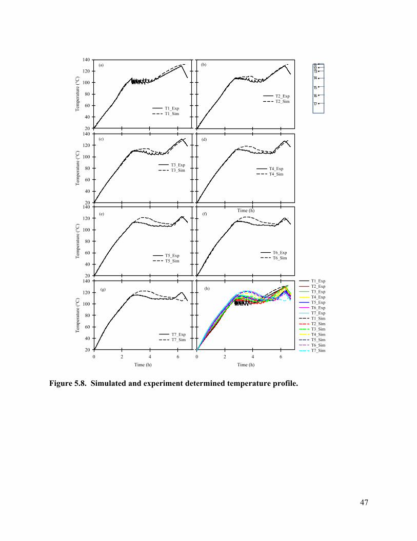
Tem

pera

ture

(°C

)

20

40

60

80

100

120

140

T1_ExpT1_Sim

T6_ExpT6_Sim

T2_ExpT2_Sim

Tem

pera

ture

(°C

)

20

40

60

80

100

120

140

T3_ExpT3_Sim

Tem

pera

ture

(°C

)

20

40

60

80

100

120

140

T5_ExpT5_Sim

Time (h)0 2 4 6

Tem

pera

ture

(°C

)

20

40

60

80

100

120

140

T7_ExpT7_Sim

Time (h)

T4_ExpT4_Sim

Time (h)0 2 4 6

T1_ExpT2_ExpT3_ExpT4_ExpT5_ExpT6_ExpT7_ExpT1_Sim T2_SimT3_Sim T4_Sim T5_SimT6_SimT7_Sim

(a) (b)

(c) (d)

(e) (f)

(g) (h)

T1

T4

T5

T3T2

T6

T7

Figure 5.8. Simulated and experiment determined temperature profile.

47

Time (h)0 1 2 3 4 5 6

Cum

ulat

ive

Con

dens

ate

Prod

uced

(mL)

0

20

40

60

80

100

SimulatedExperimental

Figure 5.9. Simulated and experimentally determined cumulative condensate produced.

Volume of condensate produced (mL)

0 10 20 30 40 50

Con

cent

ratio

n of

NaB

r (m

g/L)

0

20

40

60

80

100

120

140

160

SimulatedExperimental

Con

cent

ratio

n of

1,2

-DC

A (m

g/L)

0

200

400

600

800

1000

1200

1400

1600

1800SimulatedExperimental

(a)

(b)

Figure 5.10. Simulated and experimental effluent concentration of 1,2-DCA (a) and NaBr.

(b)

The underestimation of the steam relative permeability is supported by the results of effluent tracer concentration (Figure b). In the experiment, bromide was used as a tracer to indicate the

48

effluent steam quality, which is defined as the proportion of steam vapor in a saturated water/steam mixture. Since the bromide is nonvolatile, it can only be removed by dissolving in the liquid water, not by partitioning to the vapor phase (Chen et al. 2010). Therefore, the higher the bromide concentration in the effluent, the lower the percentage of water removed as water vapor. As shown in the Figure b, the simulated effluent bromide concentration remained at a high level until 30 mL pore water was boiled from the core. The effluent bromide concentration in the model was higher than in the experiment, suggesting a lower percentage of water removed from the core as vapor. Overall, the model and the experiment both show complete removal of the 1,2-DCA after about 45 mL of condensate has been produced from the core.

5.4 1-D Simulation without End Effects

The coupled contaminant mass and heat transfer during boiling is a very dynamic process. Small changes in boundary conditions such as heat loss at ends cause differences in temperature profile, thermodynamics, and contaminant removal. It is unavoidable to have some end effects in the experiment. To better understand the contaminant mass and heat transfer during boiling, it is helpful to conduct a simulation without experimental end effects.

The simulation without experimental end effects was conducted with a 1-D model (Figures 5.11-5.14). The Berea sandstone core was simulated with a mesh containing 48 elements and a fracture was simulated with a grid block above the subdomain of Berea sandstone. Properties such as porosity, intrinsic permeability, thermal conductivity, capillary pressure and relative permeability were identical to those used in the 2D model as described before. Heat was generated in each grid block of Berea sandstone core at a uniform rate. No flow boundary condition was applied to Berea sandstone subdomain. Deliverability model was applied to the fracture element. In the first 2.69 hours, the outlet pressure ( ) was specified as 2.047×105 Pa to simulate the state of closing the outlet valve. No fluid extraction occurs until the pressure exceeds 2.04746×105 Pa. After 2.69 hours, the outlet pressure was assigned with 1.103×105 Pa in the fracture element to simulate the state of opening the outlet valve. Both subdomains have initial water saturation of 1.0, the concentrations of 1,2-DCA and tracer were 253 mg/L and 144 mg/L (as NaBr).

Similar to the simulation before, the core was heated for 2.69 hours with both inlet and outlet valves closed. When the outlet valve was open to the atmosphere, temperature at the top of the core dropped immediately, suggesting the boiling was initiated at the top. A temperature gradient was observed while pore water in the matrix was boiled. These are larger than what we observed in the experiment. Since no heat loss was considered in this model, the duration of boiling is less than that in the experiment, and the rate of steam flow is higher. The temperature at different depths starts to increase gradually due to the drying-out of the core after heating for about 3.8 hours. The contaminant removal due to boiling in the core without end effects is shown in Figure . Before the valve was opened, contaminant was removed from the core by dissolving in the liquid water being pushed out due to the thermal expansion of fluid. After opening to the atmosphere, a high concentration of 1,2-DCA (up to 2250 mg/L) was removed, then maintained at about 700 mg/L (the concentration was 253 mg/L before heating). After boiling away 50 mL condensate, the concentration of 1,2-DCA decreases to 0.

49

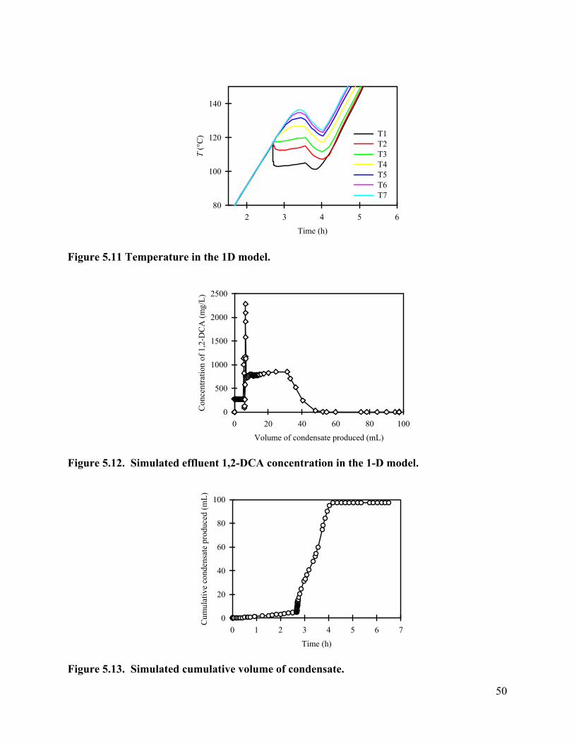
Time (h)2 3 4 5 6

T (°

C)

80

100

120

140

T1T2T3T4T5T6T7

Figure 5.11 Temperature in the 1D model.

Volume of condensate produced (mL)0 20 40 60 80 100

Con

cent

ratio

n of

1,2

-DC

A (m

g/L)

0

500

1000

1500

2000

2500

Figure 5.12. Simulated effluent 1,2-DCA concentration in the 1-D model.

Time (h)0 1 2 3 4 5 6 7

Cum

ulat

ive

cond

ensa

te p

rodu

ced

(mL)

0

20

40

60

80

100

Figure 5.13. Simulated cumulative volume of condensate.

50

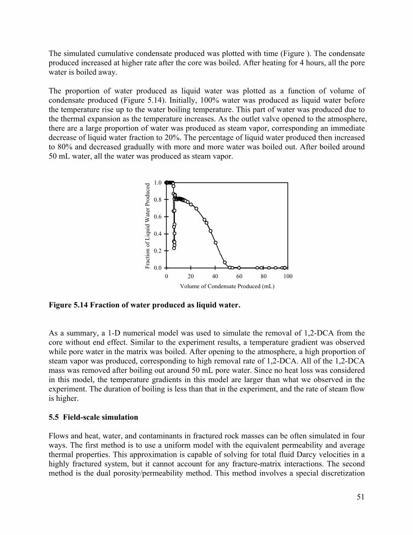
The simulated cumulative condensate produced was plotted with time (Figure ). The condensate produced increased at higher rate after the core was boiled. After heating for 4 hours, all the pore water is boiled away.

The proportion of water produced as liquid water was plotted as a function of volume of condensate produced (Figure 5.14). Initially, 100% water was produced as liquid water before the temperature rise up to the water boiling temperature. This part of water was produced due to the thermal expansion as the temperature increases. As the outlet valve opened to the atmosphere, there are a large proportion of water was produced as steam vapor, corresponding an immediate decrease of liquid water fraction to 20%. The percentage of liquid water produced then increased to 80% and decreased gradually with more and more water was boiled out. After boiled around 50 mL water, all the water was produced as steam vapor.

Volume of Condensate Produced (mL)0 20 40 60 80 100

Frac

tion

of L

iqui

d W

ater

Pro

duce

d

0.0

0.2

0.4

0.6

0.8

1.0

Figure 5.14 Fraction of water produced as liquid water.

As a summary, a 1-D numerical model was used to simulate the removal of 1,2-DCA from the core without end effect. Similar to the experiment results, a temperature gradient was observed while pore water in the matrix was boiled. After opening to the atmosphere, a high proportion of steam vapor was produced, corresponding to high removal rate of 1,2-DCA. All of the 1,2-DCA mass was removed after boiling out around 50 mL pore water. Since no heat loss was considered in this model, the temperature gradients in this model are larger than what we observed in the experiment. The duration of boiling is less than that in the experiment, and the rate of steam flow is higher.

5.5 Field-scale simulation

Flows and heat, water, and contaminants in fractured rock masses can be often simulated in four ways. The first method is to use a uniform model with the equivalent permeability and average thermal properties. This approximation is capable of solving for total fluid Darcy velocities in a highly fractured system, but it cannot account for any fracture-matrix interactions. The second method is the dual porosity/permeability method. This method involves a special discretization

51

that subdivides each normal gridblock into two volume fractions, representing the fracture and matrix, respectively. Volume fractions, permeability, capillary and relative permeability functions, porosity, and thermal properties are assigned to their domains. In the dual porosity method, the fracture volumes are globally connected in 3-D, and the matrix material is locally connected to the fracture elements. In the dual permeability method, both the fracture and matrix blocks are globally connected. The dual porosity/dual permeability methods can simulate transient multiphase fluid, heat and mass flows between the fractures and the matrix (Pruess et al. 1999), but they may not accurately resolve heat and mass fluxes between the fracture and matrix in situations where temperature, saturation, pressure and concentration gradients in the matrix are variable with time and distance into the matrix, because the state variables in the matrix block (temperature, pressure, phase saturations, concentrations) are represented by single average values over the entire matrix, and the gradients are calculated using the single average nodal distance from the matrix centroid to the fracture.

The third simulation method is the multiple interacting continua (MINC) method. This method can resolve local transient gradient of temperature, pressure, saturation, and concentration in the matrix by extending the dual porosity method to include multiple nested matrix block elements (Pruess. 1983,Pruess and Narasimhan. 1985). It subdivides a normal 3-D gridblock into a fracture element, and multiple nested matrix elements. The fracture elements are connected globally in 3-D, while the matrix elements are only locally connected to each other, and ultimately to the fracture. The individual matrix element volumes and nodal distances are based on different conceptual models of the fracture orientation and spacing. With a 3-D set of orthogonal fractures, each nested matrix element has the shape of a hollow cube, the outer matrix element is connected to the fractures, and the inner matrix elements are connected to each other in 1-D (Figure ). The nested matrix elements represent the average response of the matrix based on their distance from the nearest fracture. This method has been used to simulate energy production and mass transfer in fractured reservoirs in geothermal studies (Pruess 1983; Pruess and Narasimhan 1985; Pruess 2002). However, this method has not been applied to simulate contaminant transport in a non-isothermal process before, as far as we know.

The fourth simulation method is to model a fractured porous media with a discrete fracture-matrix model, where the fractures and matrix are fully discretized and connected in 3-D. this is the most accurate way to numerically represent a fractured porous media, however, the discretization must be limited to small domains for problems involving nonisothermal multiphase flow due to the high computational demands. Experience with these types of simulations shows that model meshes should be restricted to a few tens of thousands of gridblocks or less for reasonable run times.

In this study, we use the MINC method ( Pruess et al. 1999, Pruess and Narasimhan. 1985, Falta et al. 1995) to demonstrate the possible field scale behavior of a thermal remediation effort at a fractured site. A repeated 6-phase electrical resistance heating pattern which has an electrode array diameter of 16 m (Figure ) was considered in this field-scale simulation. From a heating and contaminant transport perspective, the hexagonal symmetry elements can be approximated as axi-symmetric cylindrical volumes bounded by insulated and no-flow boundaries. In this model, a heating depth of 20 m and a volume of about 4,020 m3 for each of these patterns were assumed (Figure ).

52

Figure 5.15. Subgridding of the method of MINC.

Figure 5.16. Six-phase electrical resistance heating pattern.

Figure 5.17. Cross-sectional view of a single element in the electrical resistance heating array used in numerical simulation.

53

The system was assumed to be composed of fractured sandstone with a 3-D set of orthogonal fractures with fracture apertures (b) of 200 µm, and a fracture spacing (D) of 1 m. The properties of the sandstone matrix were identical to the core used in the experiment, which has an intrinsic permeability of 1.5×10-13 m2 and a porosity of 0.174. Capillary and relative permeability functions used for the matrix and fracture materials were the same as those in the simulation of the laboratory experiment. The permeability of the individual fractures was estimated from the equation: /12. Overall, the equivalent continuum permeability of the rock mass would be calculated as: 2 / 1.33 10 m2. The volume fraction that these fractures occupy (calculated from 2b/D) was 0.0006 of the total volume. The initial conditions for the simulation were: a water table was 4.5 m below the ground surface, and the fractures and matrix above the water table were in gravity-capillary equilibrium with the gravity and capillary force. The initial average water saturation of the system, including the vadose zone, was 91.5%. All of the water in the matrix and fractures below the water table was initially contaminated with 253 mg/L of dissolved 1,2-DCA. An extraction well that penetrates the formation at the center of the pattern was simulated using the deliverability model as described in the equation 5.13. The productivity index (PI=6.68×10-14 m3) was calculated with

∆

(5.17)

where is the continuum permeability, ∆ is the layer thickness, is the grid block radius, is the well radius. The extraction well pump was simulated at the top of the formation, applying a vacuum of about a half atmosphere ( =5×104 Pa). Similar to the standard practice at 6-phase field sites, the ground surface was treated as a sealed and insulated boundary. To simplify the case, a no-flow boundary condition was applied to the bottom of the system, neglecting the possible heat loss from the bottom.

In the first part of the simulation, the system was uniformly heated, with the extraction well on, at 200 W/m3 for 27 days. The average temperature that is volumetrically weighted over the whole domain is plotted over time in Figure 5.18a. The average temperature increases almost linearly with time during this period, reaching 103 °C. The vacuum extraction well initially produced a mixture of air and liquid water in the first 19.6 days, during which a 1.4% of 1,2-DCA mass was removed. The well started to extract steam after heating for 19.6 days. The steam volumetric flow rate (normalizing to steam vapor density at 100 C) peaked at about 1.32×104 L/min at the end of the heating period (27 days). The peak water mass removal rate was about 8.94 kg/min. Overall, 1.5×106 kg water was removed during the heating period, accounting for 23% the initial water mass (Figure ). At the end of the heating period, 95.7% of 1,2-DCA mass was removed.

54

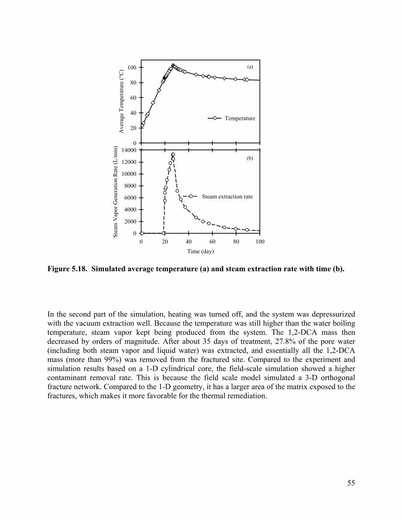
Ave

rage

Tem

pera

ture

(°C

)

0

20

40

60

80

100

Temperature

Time (day)0 20 40 60 80 100

Stea

m V

apor

Gen

erat

ion

Rat

e (L

/min

)

0

2000

4000

6000

8000

10000

12000

14000

Steam extraction rate

(a)

(b)

Figure 5.18. Simulated average temperature (a) and steam extraction rate with time (b).

In the second part of the simulation, heating was turned off, and the system was depressurized with the vacuum extraction well. Because the temperature was still higher than the water boiling temperature, steam vapor kept being produced from the system. The 1,2-DCA mass then decreased by orders of magnitude. After about 35 days of treatment, 27.8% of the pore water (including both steam vapor and liquid water) was extracted, and essentially all the 1,2-DCA mass (more than 99%) was removed from the fractured site. Compared to the experiment and simulation results based on a 1-D cylindrical core, the field-scale simulation showed a higher contaminant removal rate. This is because the field scale model simulated a 3-D orthogonal fracture network. Compared to the 1-D geometry, it has a larger area of the matrix exposed to the fractures, which makes it more favorable for the thermal remediation.

55

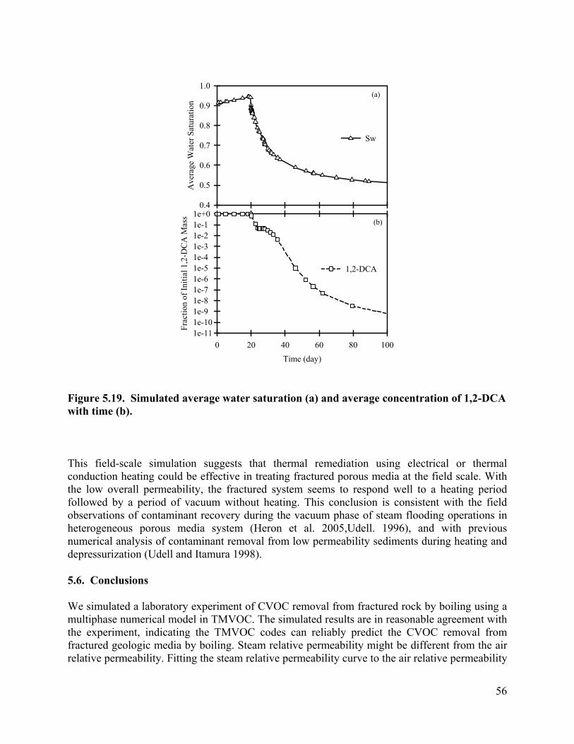
Ave

rage

Wat

er S

atur

atio

n

0.4

0.5

0.6

0.7

0.8

0.9

1.0

Sw

Time (day)0 20 40 60 80 100

Frac

tion

of In

itial

1,2

-DC

A M

ass

1e-111e-101e-91e-81e-71e-61e-51e-41e-31e-21e-11e+0

1,2-DCA

(a)

(b)

Figure 5.19. Simulated average water saturation (a) and average concentration of 1,2-DCA with time (b).

This field-scale simulation suggests that thermal remediation using electrical or thermal conduction heating could be effective in treating fractured porous media at the field scale. With the low overall permeability, the fractured system seems to respond well to a heating period followed by a period of vacuum without heating. This conclusion is consistent with the field observations of contaminant recovery during the vacuum phase of steam flooding operations in heterogeneous porous media system (Heron et al. 2005,Udell. 1996), and with previous numerical analysis of contaminant removal from low permeability sediments during heating and depressurization (Udell and Itamura 1998).

5.6. Conclusions

We simulated a laboratory experiment of CVOC removal from fractured rock by boiling using a multiphase numerical model in TMVOC. The simulated results are in reasonable agreement with the experiment, indicating the TMVOC codes can reliably predict the CVOC removal from fractured geologic media by boiling. Steam relative permeability might be different from the air relative permeability. Fitting the steam relative permeability curve to the air relative permeability

56

data might underestimate the steam relative permeability, causing higher temperature gradient, less percentage of steam vapor production, and lower rate of CVOC removal during boiling.

Further simulation of the experiment excluding the experimental end effects shows similar contaminant removal and water boiling patterns. When the temperature is above the water boiling temperature, high percentage of steam vapor is produced as the outlet open to the atmosphere, corresponding to high removal rate of CVOC. All of the 1,2-DCA is removed after boiling out half of the pore water.

MINC method has been used to simulate the contaminant removal from fractured geologic media at field scale. This method could well resolve the local transient gradient of temperature, pressure, saturation, and concentration in the matrix. The field scale simulation shows boiling is an effective mechanism for CVOC removal from fractured geologic media. After about 35 days of treatment, 27.8% of the pore water (including both steam vapor and liquid water) was extracted, and essentially all the 1,2-DCA mass (more than 99%) was removed from the fractured site.

5.7 References

A. E. Adenekan, 1992. Numerical modeling of multiphase transport of multicomponent organic contaminants and heat in the subsurfaceUniversity of California at Berkeley.

Adenekan AE, Patzek TW, Pruess K, 1993. Modeling of multiphase transport of mulitcomponent organic contaminants and heat in the subsurface: numerical model formulation. Water Resour.Res. ;29(11):3727-40.

Bachmann J, Horton R, Ren T, Ploeg RRVD, 2001. Comparison of the thermal properties of four wettable and four water-repellent soils. Soil science society of american journal ;65:1675-9.

Bristow KL, Kluitenberg GJ, Horton R, 1994. Measurement of soil properties with a dual-probe heat-pulse technique. Soil Science Society of American Journal ;58:1288-94.

Campbell GS, Calissendorff C, Williams JH, 1991. Probe for measuring soil specific heat using a heat-pulse method. Soil science society of american journal ;55:291-3.

Carslaw HS, Jaeger JC, 1959. Conduction of heat in solids. London: Oxford university press.

Chen F, Liu X, Falta RW, Murdoch LC, 2010. Experimental demonstration of contaminant removal from fractured rock by boiling. Environ.Sci.Technol. ;44:6437-42.

Chen F, Freedman DL, Falta RW, Murdoch LC. Henry's law constants of chlorinated solvents at elevated temperatures. Submitted to Environmental Science & Technology .

de Vries DA, 1952. A nonstationary method for determining thermal conductivity of soil in situ. Soil Sci. ;73:83-9.

57

Falta RW, Pruess K, Finsterle S, Battistelli A, 1995. T2VOC user's guide. ;LBL-36400.

Falta RW, Pruess K, Javandel I, Witherspoon PA, 1992a. Numerical modeling of steam injection for the removal of nonaqueous phase liquids from the subsurface 1. numerical formulation. Water Resour.Res. ;28(2):433-49.

Falta RW, Pruess K, Javandel I, Witherspoon PA, 1992b. Numerical modeling of steam injection for the removal of nonaqueous phase liquids from the subsurface 2. code validation and application. Water Resour.Res. ;28(2):451-65.

Gauglitz PA, Roberts JS, Bergsman TM, Schalla R, Caley SM, Schlender MH, et al, 1994. Six-phase soil heating for enhanced removal of contaminants: Volatile organic compounds in non-arid soils integrated demonstration, Savannah River Site.

Gossett JM, 1987. Measurement of Henry's law constants for C1 and C2 chlorinated hydrocarbons. Environmental Science and Technology ;21:202-8.

Gudbjerg J, Sonnenborg TO, Jensen KH, 2004. Remediation of NAPL below the water table by steam-induced heat conduction. J.Contam.Hydrol. ;72:207-25.

Heron G, Christensen TH, Enfield CG, 1998a. Henry's law constant for trichloroethylene between 10 and 95 °C. Environ.Sci.Technol. ;32(10):1433-7.

Heron G, Zutphen MV, Christensen TH, Enfield CG, 1998b. Soil heating for enhanced remediation of chlorinated solvents: A laboratory study on resistive heating and vapor extraction in a silty, low-permeable soil contaminated with trichloroethylene. Environ.Sci.Technol. ;32(10):1474-81.

Heron G, Carroll S, Nielsen SG, 2005. Full-scale removal of DNAPL constituents using steam-enhanced extraction and electrical resistance heating. Ground Water Monitoring & Remediation ;25(4):92-107.

Heron G, Parker K, Galligan J, Holmes TC, 2009. Thermal treatment of eight CVOC source zones to near nondetect concentrations. Ground Water Monitoring & Remediation ;29(3):56-65.

Horne RN, Satik C, Mahiya G, Li K, Ambusso W, Tovar R, et al, 2000. Steam-water relative permeability.

Smith WE, editor, 1965. Application of the theory of heat conduction to geothermal measurements. Terrestrial Heat Flow: American Geophysical Union.

Kluitenberg GJ, Ham JM, Bristow KL, 1993. Error analysis of the heat pulse method for measuring soil volumetric heat capacity. Soil Sci.Soc.Am.J. ;57:1444-51.

58

Knight JH, Jin W, Kluitenberg GJ, 2007. Sensitivity of the dual-probe heat-pulse method to spatial variations in heat capacity and water content. Vadose Zone Journal ;6(4):746-58.

Kubičár Ľ, Vretenár V, Boháč V, Tiano P, 2006. Thermophysical analysis of sandstone by pulse transient method. Int.J.Thermophys. ;27(1):220-34.

Lewis TJ, Villinger H, Davis EE, 1993. Thermal conductivity measurement of rock fragments using a pulsed needle probe. Canadian Journal of Earth Sciences ;30:480-5.

Li K, Horne RN, 2004. Steam-water and air-water capillary pressures: Measurement and comparison. J Can Pet Technol ;43(7):24-30.

Lu S, Ren T, Gong Y, Horton R, 2007. An improved model for predicting soil thermal conductivity from water content at room temperature. Soil Sci.Soc.Am.J. ;71:8-14.

Lubimova HA, Lusova LM, Firsov FV, Starkova GN, Shushpanov AP, 1961. Determination of surface heat flow in Mazesta. Annales geophysicae ;14:157-67.

Muñoz JJ, Alonso EE, Lloret A, 2009. Thermo-hydraulic characterisation of soft rock by means of heating pulse tests. Geotechnique ;59(4):293-306.

Ochs SO, Hodges RA, Falta RW, Kmetz TF, Kupar JJ, Brown NN, et al, 2003. Predicted heating patterns during steam flooding of coastal plain sediments at the Savannah River Site. Environmental and Engineering Geoscience ;9(1):51-69.

Parker BL, McWhorter DB, Cherry JA, 1997. Diffusive loss of non-aqueous phase organic solvents from idealized fracture networks in geologic media. Ground Water ;36(6):1077-88.

Parker BL, McWhorter DB, Cherry JA, 1994. Diffusive disappearance of immiscible-phase organic liquids in fractured geologic media. Ground Water ;32(4):805-20.

Parker JC, Lenhard RJ, Kuppusamy T, 1987. A parametric model for constitutive properties governing multiphase flow in porous media. Water Resour.Res. ;23(4):618-24.

TMVOC, a simulator for multiple volatile organic chemicals. 2003. TOUGH Symposium 2003 Lawrenece Berkeley National Laboratory, Berkeley, California.

Pruess K, Battistelli A, 2002. TMVOC, A numerical simulator for three-phase non-isothermal flows of multicomponent hydrocarbon mixtures in saturated-unsaturated heterogeneous media. ;LBNL-49375.

Pruess K, 2002. Numerical simulation of multiphase tracer transport in fractured geothermal reservoirs. Geothermics ;31:475-99.

Pruess K, Oldenburg C, Moridis G, 1999. TOUGH2 user's guide, version 2.0.

59

Pruess K, 1983. Heat transfer in fractured geothermal reservoirs with boiling. Water Resour.Res. ;19(1):201-8.

Pruess K, Narasimhan TN, 1985. A practical method for modeling fluid and heat flow in fractured porous media. Society of Petroleum Engineers Journal ;25(1):14-26.

Reynolds DA, Kueper BH, 2002. Numerical examination of the factors controlling DNAPL migration through a single fracture. Groundwater ;40(4):368-77.

Reynolds DA, Kueper BH, 2001. Multiphase flow and transport in fractured clay/sand sequences. J.Contam.Hydrol. ;51:41-62.

Roland U, Buchenhorst D, Holzer F, Kopinke FD, 2008. Engineering aspects of radio-wave heating for soil remediation and compatibility with biodegradation. Environ.Sci.Technol. ;42(4):1232-7.

Roland U, Bergmann S, Holzer F, Kopinke F, 2010. Influence of in situ steam formation by radio frequency heating on thermodesorption of hydrocarbons from contaminated soil. Environ.Sci.Technol. ;44:9502-8.

Ross B, Lu N, 1999. Dynamics of DNAPL penetration into fractured porous media. Groundwater ;37(1):140-7.

Tarara JM, Ham JM, 1997. Measuring soil water content in the laboratory and field with dual-probe heat-capacity sensors. Agron.J. ;89(4):535-42.

Tse KKC, Liou T, Lo S, 2006. Numerical simulation of a steam-injection pilot study for a PCP-contaminated aquifer. Environ.Sci.Technol. ;40:4292-9.

Udell KS, 1996. Heat and mass transfer in clean-up of underground toxic wastes. Annual Review of Heat Transfer ;7:333-405.

Udell KS, Itamura MT, 1998. Removal of dissolved solvents from heated heterogeneous soils during depressurization. Columbus, Ohio: Battelle Press.

van Genuchten MT, 1980. A closed-form equation for predicting the hydraulic conductivity of unsaturated soils. Soil Sci.Soc.Am.J. ;44:892-8.

Enhancement of steam phase relative permeability due to phase transformation effects in porous media. 1986. Proceedings, Eleventh Workshop Geothermal Reservoir Engineering; Jan 21-23, 1986; .

Verma AK, 1986. Effects of phase transformation on steam water relative permeability.

Welch SM, Kluitenberg GJ, Bristow KL, 1996. Rapid numerical estimation of soil thermal properties for a broad class of heat-pulse emitter geometries. Meas Sci Technol ;7:932-8.

60

Zhu S, Ramaswamy HS, Marcotte M, Chen C, Shao Y, Bail AL, 2007. Evaluation of thermal properties of food materials at high pressures using a dual-needle line-heat-source method. J.Food Sci. ;72(2):49-56.

61

6. Field Scale Simulations of Thermal Remediation of Fractured Rocks (to be submitted to the Journal of Contaminant Hydrology, 2011)

6.1. Introduction

Contaminant removal from fractured rock by boiling has recently been demonstrated in a laboratory experiment (Chen et al. 2010; Chapter 3). After boiling away about 1/3 of the pore volume of water from a contaminated sandstone core, approximately 100% recovery of 1,2-dichloroethane (1,2-DCA) was achieved (Chen et al. 2010). The T2VOC and TMVOC multiphase flow heat and mass transfer codes have been widely used for simulation of multiphase flow with single and multiple volatile organic chemical(s) (Falta et al. 1995, Pruess and Battistelli, 2003 ,Tse et al., 2006). They were validated with experimental results for a variety of isothermal and non-isothermal problems that are similar to this problem (Adenekan, 1992, Adenekan et al., 1993, Falta et al., 1992, Gudbjerg et al., 2004, and Ochs et al., 2003). The reliability of the codes in predicting the contaminant mass transfer between matrix blocks and fractures has been further established by comparing simulations with the experimental results, and they are in reasonable agreement (Chapter 5). However, there were limited studies on simulation of contaminant mass transfer from fractured geologic media with boiling at the scale of typical field applications. It is not known how the geologic and flow parameters such as matrix permeability, fracture aperture, and fracture spacing affect the performance of thermal remediation. Also, the effects of some operational and design parameters and strategies such as the diameter of heating pattern, the magnitude of the vacuum in extraction wells, and cycling of heating and extraction are not well understood.

In this section, we conduct sensitivity analysis over a series of matrix and fracture properties (matrix permeability, fracture aperture, and fracture spacing), and design and operational parameters (diameter of heating pattern, extent of vacuum, cycling heating and extraction).

6.2. Methods

6.2.1.Multiple Interacting Continua

As in the previous Chapter, MINC method, as an extension of the dual porosity concept, is used for modeling flow in fractured porous media (Pruess and Battistelli, 2002, Pruess and Narasimhan, 1985). Similar to the dual porosity method, the MINC method embeds the low-permeable matrix blocks in a network of interconnected fractures. Global flow occurs only through the fracture system, while the matrix is locally connected to the fracture, and exchanges fluid (or heat) locally with the fracture system. The fluid (heat) flow between the fracture and matrix is driven by the difference in pressures (or temperatures) between them. The MINC method is capable of resolving the gradients with a special discretization, appropriately sub-discretizing a normal matrix block into multiple subgrids (Figure ). The fluid and heat flow between the fractures and the matrix blocks can then be modeled locally (within each main grid-block) as a one-dimensional process.

62

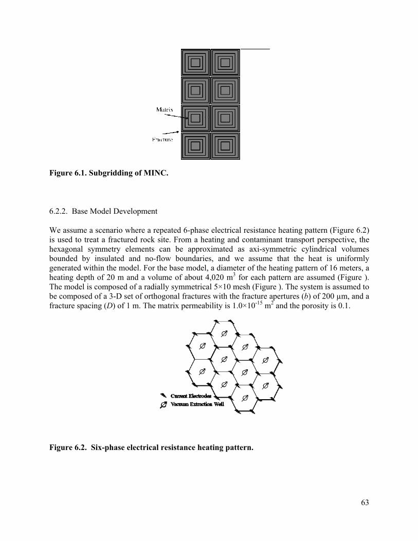
Figure 6.1. Subgridding of MINC.

6.2.2. Base Model Development

We assume a scenario where a repeated 6-phase electrical resistance heating pattern (Figure 6.2) is used to treat a fractured rock site. From a heating and contaminant transport perspective, the hexagonal symmetry elements can be approximated as axi-symmetric cylindrical volumes bounded by insulated and no-flow boundaries, and we assume that the heat is uniformly generated within the model. For the base model, a diameter of the heating pattern of 16 meters, a heating depth of 20 m and a volume of about 4,020 m3 for each pattern are assumed (Figure ). The model is composed of a radially symmetrical 5×10 mesh (Figure ). The system is assumed to be composed of a 3-D set of orthogonal fractures with the fracture apertures (b) of 200 µm, and a fracture spacing (D) of 1 m. The matrix permeability is 1.0×10-15 m2 and the porosity is 0.1.

Figure 6.2. Six-phase electrical resistance heating pattern.

63

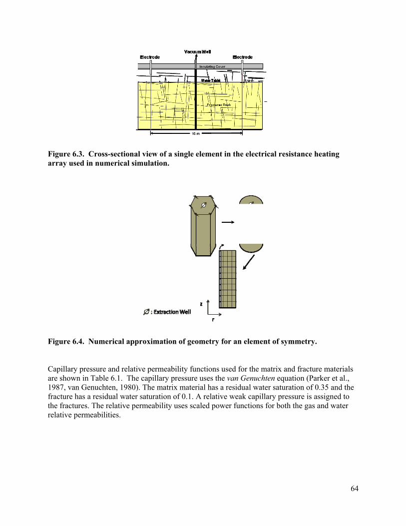
Figure 6.3. Cross-sectional view of a single element in the electrical resistance heating array used in numerical simulation.

Figure 6.4. Numerical approximation of geometry for an element of symmetry.

Capillary pressure and relative permeability functions used for the matrix and fracture materials are shown in Table 6.1. The capillary pressure uses the van Genuchten equation (Parker et al., 1987, van Genuchten, 1980). The matrix material has a residual water saturation of 0.35 and the fracture has a residual water saturation of 0.1. A relative weak capillary pressure is assigned to the fractures. The relative permeability uses scaled power functions for both the gas and water relative permeabilities.

64

Table 6.2 Capillary pressure and relative permeability

Fracture Capillary pressure 1 11

/

1/

=0.1, n= .00 ‐ =23 , m=1 1/n, = 8

Relative permeability 1 ; 1

=0.1, 0, == 2

Matrix Capillary pressure 1 11

/

1/

=0.35, n=2.00, m=1-1/n, = =0.5

Relative permeability 1 ; 1

=0.35, =0, =3

The permeability of the individual fractures is estimated from the equation: /12 . Assuming a 3D orthogonal network of fractures, the equivalent continuum permeability of the rock mass is calculated as: 2 / 1.33 10 m2. The volume fraction that the fractures occupy is assigned to be 0.01 of the total volume. Although it is a little higher than the true value calculated from 3 / , its effect to the simulated results is negligible, and it allows the model to run more smoothly (Pruess and Narasimhan, 1985).

The initial conditions for the base simulation consist of a water table 4.5 m below the ground surface, with fractures and matrix above the water table in gravity-capillary. The initial average water saturation of the system, including the vadose zone, is 97.9%. All of the water in the matrix and fractures below the water table is initially contaminated with 7.53 mg/L of dissolved 1,2-DCA. An extraction well that penetrates the formation at the center of the pattern is simulated using a well deliverability mod l ss Be (Prue and attistelli, 2002):

(6.1

The productivity index is calculated with

∆

(6.2)

65

where is effective continuum permeability, ∆ is the layer thickness, is the grid block centroid radius, and is the well radius. The extraction well pump was simulated at the top of

the formation, applying a vacuum of a half an atmosphere ( =5×104 Pa). Similar to the standard practice at 6-phase field sites, the ground surface was treated as a sealed and insulated boundary. To simplify the case, a no-flow boundary condition was applied to the bottom of the system, neglecting the possible heat loss from the bottom.

6.3. Results

For the base model, the saturated zone is heated at a uniform rate of 200 W/m2 with the extraction well on for 18 days. After that, the heater is turned off and the extraction well is left on with a vacuum of 0.5 atm. Overall, this setup is very similar to the one described at the end of Chapter 5, and the general behavior is similar.

6.3.1. Effect of Chemical Properties

Different chlorinated solvents might have a different response for thermal remediation. Chlorinated solvents such as 1,2-dichloroethane (1,2-DCA), chloroform (CF), carbon tetrachloride (CT), tetrachloroethylene (PCE), trichloroethylene (TCE) are among the most frequently detected contaminants at contaminated sites. Recently, the Henry’s law constants and aqueous solubility of these chemicals were measured as functions of temperature (Chapter 4). Here we simulate the removal of these chemical from the fractured site as described in the base model. The temperature dependency of the Henry’s law constant has been considered in the model by fitting to the measured data from Chapter 4. For different chemicals, it is not surprising that the patterns of average temperature (Figure ) and the average water saturation (Figure ) changes with time are similar because the properties of chemicals have little effects on the water boiling. However, under the same boiling conditions, the contaminant removal rates vary for different chemicals (Figure 6.7). Among these chemicals, carbon tetrachloride has the best removal rate, followed by tetrachloroethylene, trichloroethylene, chloroform, and 1,2-dichloroethane, respectively. The order is the same as the magnitude of Henry’s law constants for these chemicals. The higher the Henry’s law constant, the higher the contaminant removal rate.

Figure 6.5 Average temperatures for the cases contaminated with different chemicals

66

Figure 6.6. Average water saturations for the cases contaminated with different chemicals

Figure 6.7. Fraction of initial contaminant mass for the cases contaminated with different chemicals

6.3.2. Effect of Diameter of Heating Pattern

The size of heating pattern is important for thermal remediation. Diameters of 4, 8, 16, and 32 meters have been simulated to demonstrate the behavior of contaminant removal. The average temperature is plotted as a function of time in Figure 6.8. The average water saturation is shown in Figure , and contaminant removal efficiencies are shown in figure 6.10.

For a diameter of 4 meters, the average temperature increases to a maximum of only 85.75 ˚C after heating for 13 days due to boiling. Boiling occurs earlier, and at a lower temperature in this

67

case, because the system is more effectively depressurized by its close proximity to the extraction well. As boiling occurs and steam is extracted, the temperature decreases slightly to 82.9 ˚C by day 18, when the heater is turned off. After 18 days, the heaters are turned off but the extraction well remains on, and the temperature decreases quickly to 75 ˚C by day 23, and then stabilizes at this value.

The initial average water saturation is 0.978. Heating for 13.32 days, the water saturation increases slightly to 0.982. The increased water saturation at early times is caused by thermal expansion. Further heating and extracting causes the water boiling. The average water saturation decreases to 0.632 in day 18, and 0.546 in day 23 (Figure ). In the first 13.6 days, about 14.2% of the 1,2-DCA mass removed is due to the extraction of liquid water. From days 13.6 to 23, 73.8% 1,2-DCA mass is removed. The steam vapor extraction rate reaches 4.65×103 L/min at day 13.3, and gradually decreases to zero in day 28 (Figure 6.11).

Figure 6.8. Average temperatures for the cases with different diameters of heating pattern.

Figure 6.9. Average water saturations for cases with different diameters of heating pattern.

68

Figure 6.10. Fraction of initial 1,2-DCA mass remaining for cases with different diameters of heating pattern.

Figure 6.11. Vapor extraction rate for heating diameter of 4 m.

For a diameter of 8 meters, the average temperature increases to 85.7 ˚C after heating for 13.3 days, when boiling near the well begins. It continues to increase to 93.2 ˚C at 18 days at which point the heater is turned off. After the heater is turned off, it decreases to 79.6 in day 48, and then stabilizes at that temperature (Figure 6.8).

The initial average water saturation was 0.978. During the first 13.3 days, the average water saturation increases to 0.981 due to thermal expansion. Then it decreases to 0.754 by day 18, and 0.587 in day 48 (Figure 6.9). About 2% of 1,2-DCA mass is removed due to extraction of liquid water during the first 10 days. From day 10 to 18, 69.2% 1,2-DCA mass is removed, primarily in the vapor phase. Further extraction corresponding to another 8.8% removal of 1,2-DCA mass occurs after the heater is turned off (Figure 6.10). After 48 days, there is not much further

69

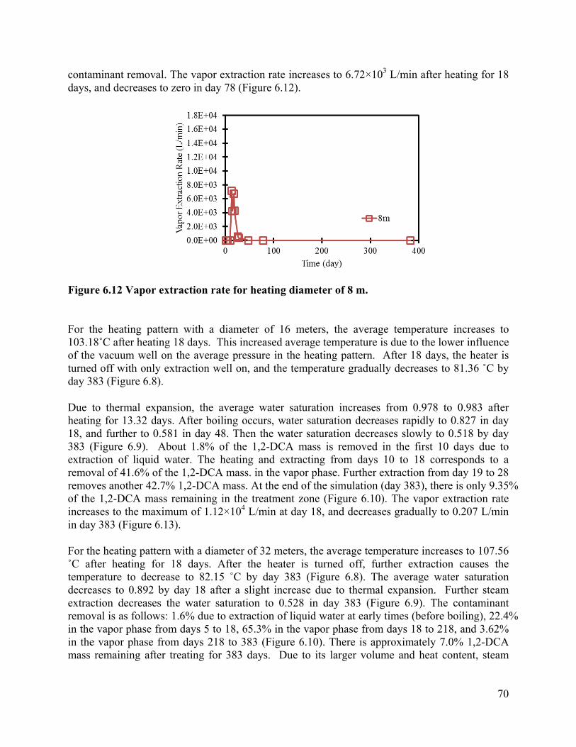
contaminant removal. The vapor extraction rate increases to 6.72×103 L/min after heating for 18 days, and decreases to zero in day 78 (Figure 6.12).

Figure 6.12 Vapor extraction rate for heating diameter of 8 m.

For the heating pattern with a diameter of 16 meters, the average temperature increases to 103.18˚C after heating 18 days. This increased average temperature is due to the lower influence of the vacuum well on the average pressure in the heating pattern. After 18 days, the heater is turned off with only extraction well on, and the temperature gradually decreases to 81.36 ˚C by day 383 (Figure 6.8).

Due to thermal expansion, the average water saturation increases from 0.978 to 0.983 after heating for 13.32 days. After boiling occurs, water saturation decreases rapidly to 0.827 in day 18, and further to 0.581 in day 48. Then the water saturation decreases slowly to 0.518 by day 383 (Figure 6.9). About 1.8% of the 1,2-DCA mass is removed in the first 10 days due to extraction of liquid water. The heating and extracting from days 10 to 18 corresponds to a removal of 41.6% of the 1,2-DCA mass. in the vapor phase. Further extraction from day 19 to 28 removes another 42.7% 1,2-DCA mass. At the end of the simulation (day 383), there is only 9.35% of the 1,2-DCA mass remaining in the treatment zone (Figure 6.10). The vapor extraction rate increases to the maximum of 1.12×104 L/min at day 18, and decreases gradually to 0.207 L/min in day 383 (Figure 6.13).

For the heating pattern with a diameter of 32 meters, the average temperature increases to 107.56 ˚C after heating for 18 days. After the heater is turned off, further extraction causes the temperature to decrease to 82.15 ˚C by day 383 (Figure 6.8). The average water saturation decreases to 0.892 by day 18 after a slight increase due to thermal expansion. Further steam extraction decreases the water saturation to 0.528 in day 383 (Figure 6.9). The contaminant removal is as follows: 1.6% due to extraction of liquid water at early times (before boiling), 22.4% in the vapor phase from days 5 to 18, 65.3% in the vapor phase from days 18 to 218, and 3.62% in the vapor phase from days 218 to 383 (Figure 6.10). There is approximately 7.0% 1,2-DCA mass remaining after treating for 383 days. Due to its larger volume and heat content, steam

70

vapor production from the well is maintained for a longer period of time in this larger pattern, and the peak steam production rate is larger than that seen in the other patterns (Figure 6.14).

Figure 6.13. Vapor extraction rate for heating diameter of 16 m.

Figure 6.14. Vapor extraction rate for heating diameter of 32 m.

The sensitivity analysis on the diameter of heating pattern shows that as long as the fracture network is well connected, that effective contaminant removal can occur at a variety of heating pattern sizes. For a smaller diameter, the extraction well has stronger influence on the treatment zone. Water boils at lower temperatures due to the decreased pressure caused by extraction. The disadvantage of this is that a higher percentage of heat is extracted out of the treatment zone at early times, causing the boiling to cease earlier after the heater is turned off. The contaminant mass from farther regions re-contaminates the zones that are close to the extraction well.

71

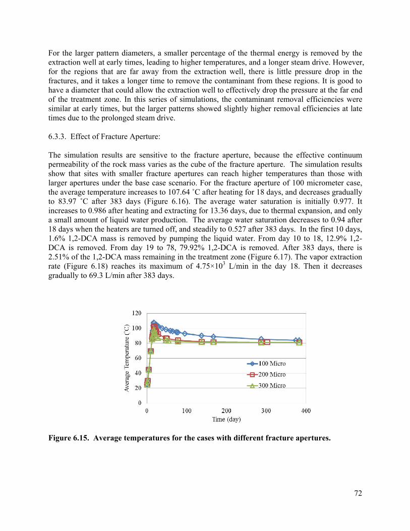
For the larger pattern diameters, a smaller percentage of the thermal energy is removed by the extraction well at early times, leading to higher temperatures, and a longer steam drive. However, for the regions that are far away from the extraction well, there is little pressure drop in the fractures, and it takes a longer time to remove the contaminant from these regions. It is good to have a diameter that could allow the extraction well to effectively drop the pressure at the far end of the treatment zone. In this series of simulations, the contaminant removal efficiencies were similar at early times, but the larger patterns showed slightly higher removal efficiencies at late times due to the prolonged steam drive.

6.3.3. Effect of Fracture Aperture:

The simulation results are sensitive to the fracture aperture, because the effective continuum permeability of the rock mass varies as the cube of the fracture aperture. The simulation results show that sites with smaller fracture apertures can reach higher temperatures than those with larger apertures under the base case scenario. For the fracture aperture of 100 micrometer case, the average temperature increases to 107.64 ˚C after heating for 18 days, and decreases gradually to 83.97 ˚C after 383 days (Figure 6.16). The average water saturation is initially 0.977. It increases to 0.986 after heating and extracting for 13.36 days, due to thermal expansion, and only a small amount of liquid water production. The average water saturation decreases to 0.94 after 18 days when the heaters are turned off, and steadily to 0.527 after 383 days. In the first 10 days, 1.6% 1,2-DCA mass is removed by pumping the liquid water. From day 10 to 18, 12.9% 1,2-DCA is removed. From day 19 to 78, 79.92% 1,2-DCA is removed. After 383 days, there is 2.51% of the 1,2-DCA mass remaining in the treatment zone (Figure 6.17). The vapor extraction rate (Figure 6.18) reaches its maximum of 4.75×103 L/min in the day 18. Then it decreases gradually to 69.3 L/min after 383 days.

Figure 6.15. Average temperatures for the cases with different fracture apertures.

72

Figure 6.16. Average water saturations for the cases with different fracture apertures.

Figure 6.17. Fraction of the initial 1,2-DCA mass remaining in the cases with different fracture apertures.

Figure 6.18. Vapor extraction rate for the case with fracture aperture of 100 micrometers.

73

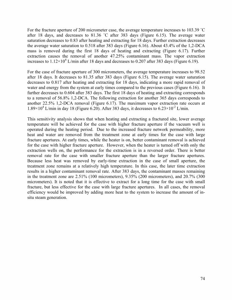
For the fracture aperture of 200 micrometer case, the average temperature increases to 103.39 ˚C after 18 days, and decreases to 81.36 ˚C after 383 days (Figure 6.15). The average water saturation decreases to 0.83 after heating and extracting for 18 days. Further extraction decreases the average water saturation to 0.518 after 383 days (Figure 6.16). About 43.4% of the 1,2-DCA mass is removed during the first 18 days of heating and extracting (Figure 6.17). Further extraction causes the removal of another 47.25% contaminant mass. The vapor extraction increases to 1.12×104 L/min after 18 days and decreases to 0.207 after 383 days (Figure 6.19).

For the case of fracture aperture of 300 micrometers, the average temperature increases to 98.52 after 18 days. It decreases to 81.35 after 383 days (Figure 6.15). The average water saturation decreases to 0.817 after heating and extracting for 18 days, indicating a more rapid removal of water and energy from the system at early times compared to the previous cases (Figure 6.16). It further decreases to 0.604 after 383 days. The first 18 days of heating and extracting corresponds to a removal of 56.8% 1,2-DCA. The following extraction for another 365 days corresponds to another 22.5% 1,2-DCA removal (Figure 6.17). The maximum vapor extraction rate occurs at 1.89×104 L/min in day 18 (Figure 6.20). After 383 days, it decreases to 6.23×10-2 L/min.

This sensitivity analysis shows that when heating and extracting a fractured site, lower average temperature will be achieved for the case with higher fracture aperture if the vacuum well is operated during the heating period. Due to the increased fracture network permeability, more heat and water are removed from the treatment zone at early times for the case with large fracture apertures. At early times, while the heater is on, better contaminant removal is achieved for the case with higher fracture aperture. However, when the heater is turned off with only the extraction wells on, the performance for the extraction is in a reversed order. There is better removal rate for the case with smaller fracture aperture than the larger fracture apertures. Because less heat was removed by early-time extraction in the case of small aperture, the treatment zone remains at a relatively high temperature. In this case, the later time extraction results in a higher contaminant removal rate. After 383 days, the contaminant masses remaining in the treatment zone are 2.51% (100 micrometers), 9.35% (200 micrometers), and 20.7% (300 micrometers). It is noted that it is effective to extract for a long time for the case with small fracture, but less effective for the case with large fracture apertures. In all cases, the removal efficiency would be improved by adding more heat to the system to increase the amount of in-situ steam generation.

74

Figure 6.19. Vapor extraction rate for the case with fracture aperture of 200 micrometers.

Figure 6.20. Vapor extraction rate for the case with fracture aperture of 300 micrometers.

6.3.4. Effect of Fracture Spacing

The base model considered a 3D orthogonal network of fractures with a uniform 1 m spacing. Here, we evaluate cases with one-half, and twice this fracture spacing. These different cases are constructed by generating new MINC grids to reflect the different fracture-matrix relationships. Changing the fracture spacing changes the effective permeability of the fracture network, and it alters the fracture-matrix geometry by affecting the average proximity of the matrix volumes to the fractures.

75

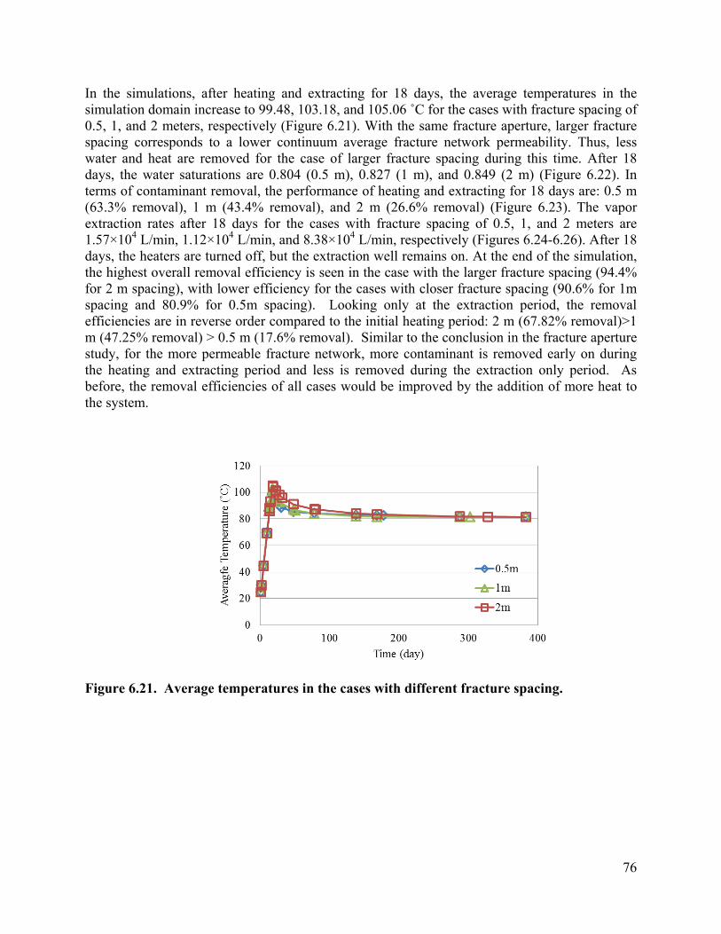
In the simulations, after heating and extracting for 18 days, the average temperatures in the simulation domain increase to 99.48, 103.18, and 105.06 ˚C for the cases with fracture spacing of 0.5, 1, and 2 meters, respectively (Figure 6.21). With the same fracture aperture, larger fracture spacing corresponds to a lower continuum average fracture network permeability. Thus, less water and heat are removed for the case of larger fracture spacing during this time. After 18 days, the water saturations are 0.804 (0.5 m), 0.827 (1 m), and 0.849 (2 m) (Figure 6.22). In terms of contaminant removal, the performance of heating and extracting for 18 days are: 0.5 m (63.3% removal), 1 m (43.4% removal), and 2 m (26.6% removal) (Figure 6.23). The vapor extraction rates after 18 days for the cases with fracture spacing of 0.5, 1, and 2 meters are 1.57×104 L/min, 1.12×104 L/min, and 8.38×104 L/min, respectively (Figures 6.24-6.26). After 18 days, the heaters are turned off, but the extraction well remains on. At the end of the simulation, the highest overall removal efficiency is seen in the case with the larger fracture spacing (94.4% for 2 m spacing), with lower efficiency for the cases with closer fracture spacing (90.6% for 1m spacing and 80.9% for 0.5m spacing). Looking only at the extraction period, the removal efficiencies are in reverse order compared to the initial heating period: 2 m (67.82% removal)>1 m (47.25% removal) > 0.5 m (17.6% removal). Similar to the conclusion in the fracture aperture study, for the more permeable fracture network, more contaminant is removed early on during the heating and extracting period and less is removed during the extraction only period. As before, the removal efficiencies of all cases would be improved by the addition of more heat to the system.

Figure 6.21. Average temperatures in the cases with different fracture spacing.

76

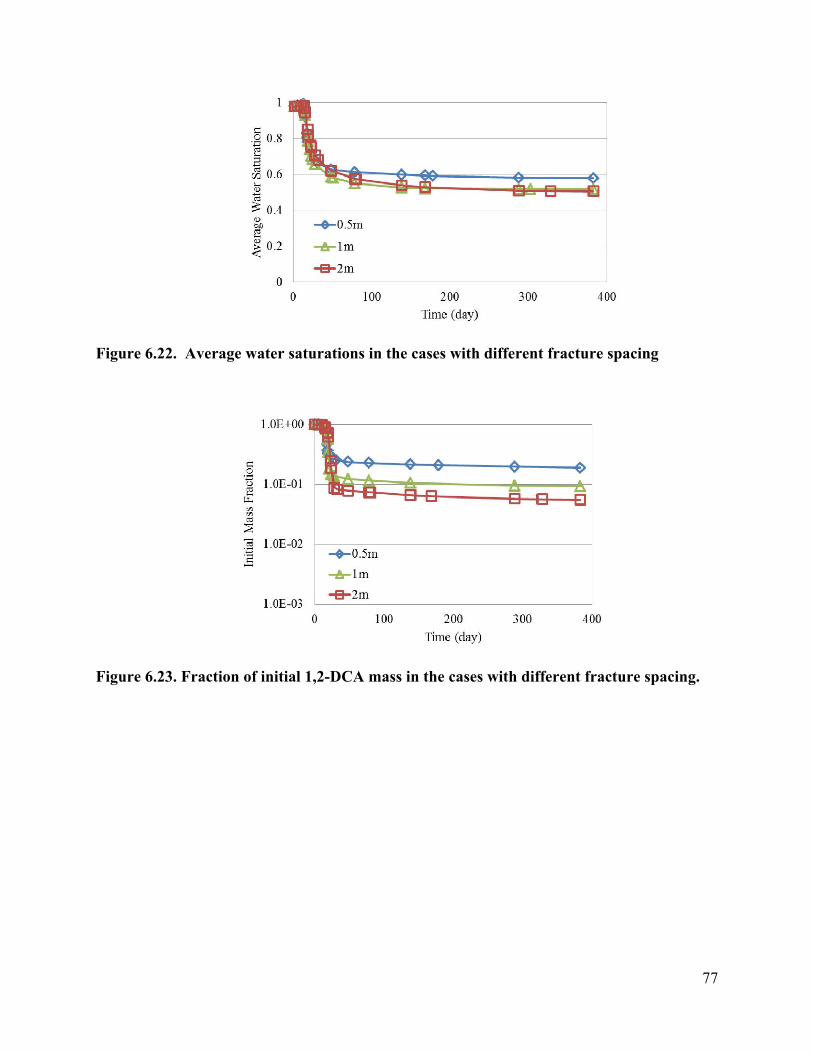
Figure 6.22. Average water saturations in the cases with different fracture spacing

Figure 6.23. Fraction of initial 1,2-DCA mass in the cases with different fracture spacing.

77

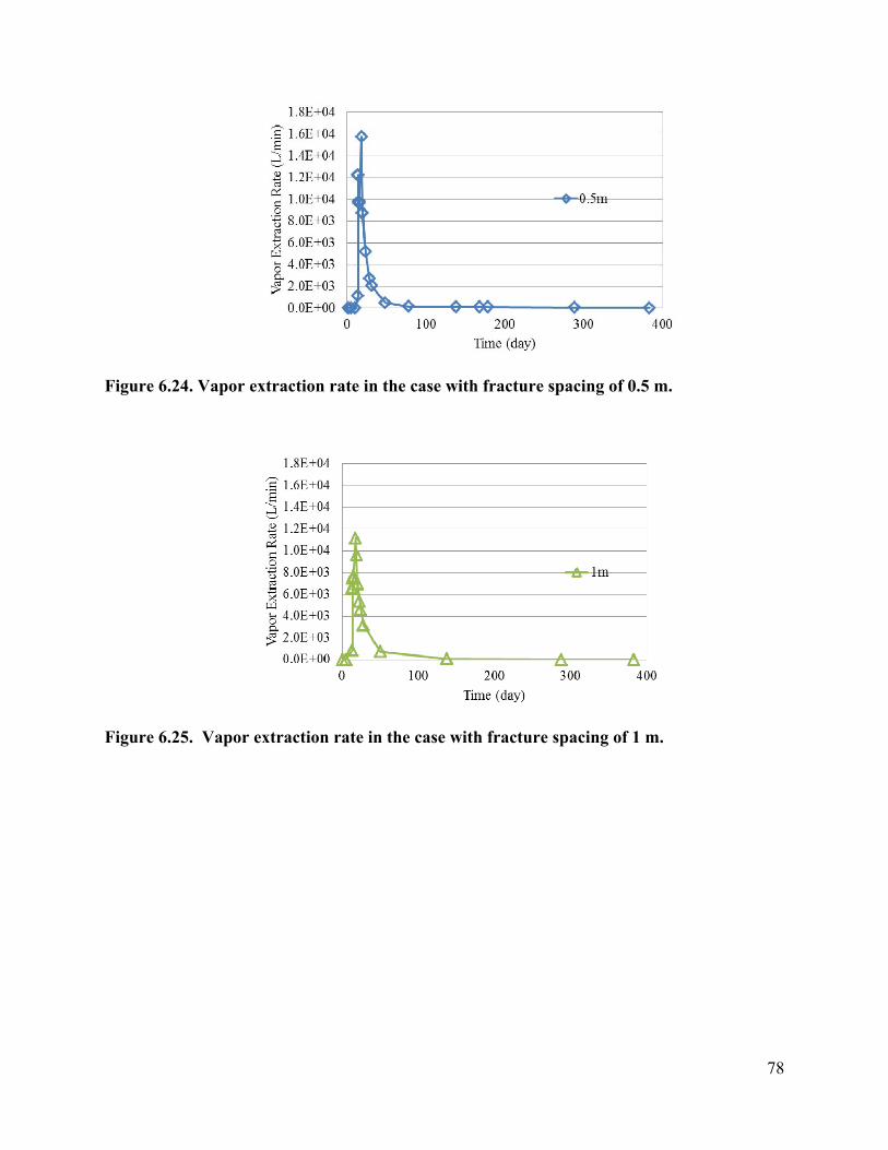
Figure 6.24. Vapor extraction rate in the case with fracture spacing of 0.5 m.

Figure 6.25. Vapor extraction rate in the case with fracture spacing of 1 m.

78

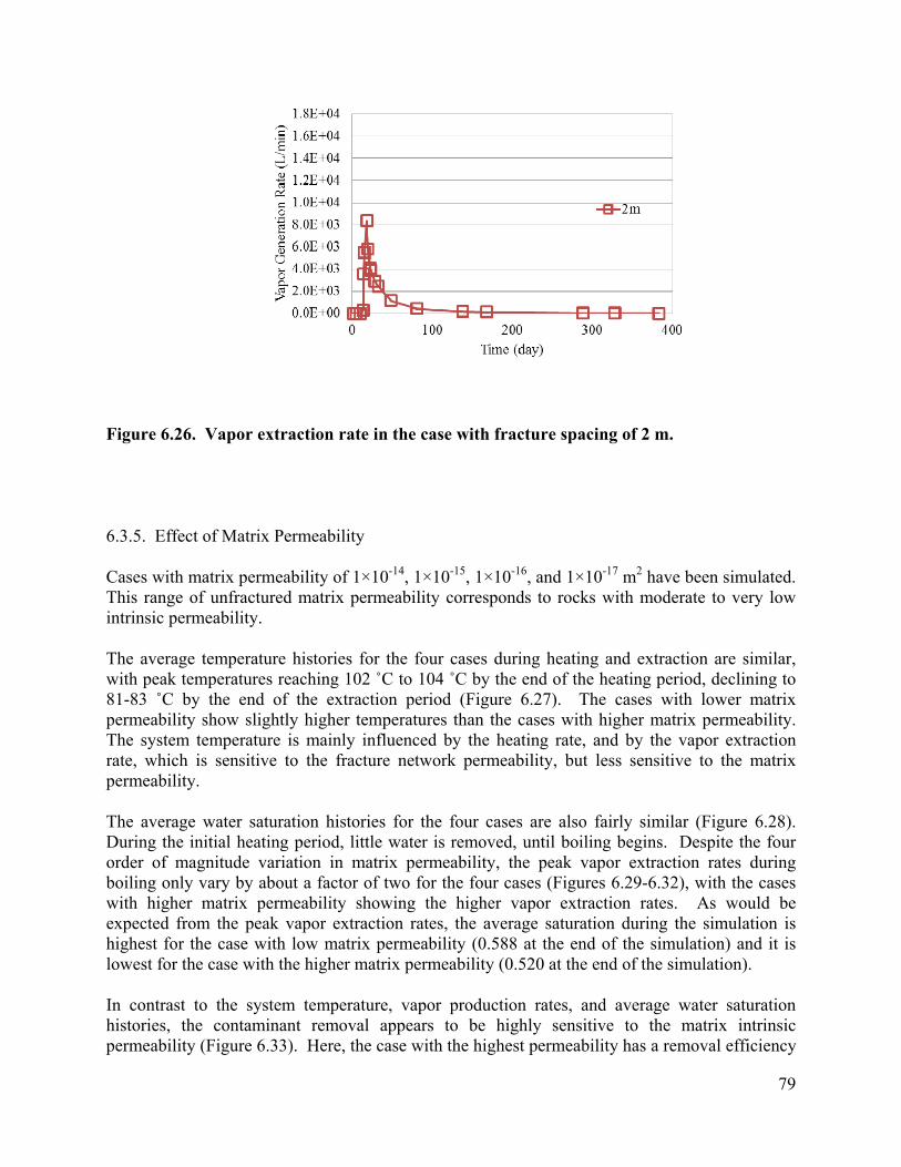
Figure 6.26. Vapor extraction rate in the case with fracture spacing of 2 m.

6.3.5. Effect of Matrix Permeability

Cases with matrix permeability of 1×10-14, 1×10-15, 1×10-16, and 1×10-17 m2 have been simulated. This range of unfractured matrix permeability corresponds to rocks with moderate to very low intrinsic permeability.

The average temperature histories for the four cases during heating and extraction are similar, with peak temperatures reaching 102 ˚C to 104 ˚C by the end of the heating period, declining to 81-83 ˚C by the end of the extraction period (Figure 6.27). The cases with lower matrix permeability show slightly higher temperatures than the cases with higher matrix permeability. The system temperature is mainly influenced by the heating rate, and by the vapor extraction rate, which is sensitive to the fracture network permeability, but less sensitive to the matrix permeability.

The average water saturation histories for the four cases are also fairly similar (Figure 6.28). During the initial heating period, little water is removed, until boiling begins. Despite the four order of magnitude variation in matrix permeability, the peak vapor extraction rates during boiling only vary by about a factor of two for the four cases (Figures 6.29-6.32), with the cases with higher matrix permeability showing the higher vapor extraction rates. As would be expected from the peak vapor extraction rates, the average saturation during the simulation is highest for the case with low matrix permeability (0.588 at the end of the simulation) and it is lowest for the case with the higher matrix permeability (0.520 at the end of the simulation).

In contrast to the system temperature, vapor production rates, and average water saturation histories, the contaminant removal appears to be highly sensitive to the matrix intrinsic permeability (Figure 6.33). Here, the case with the highest permeability has a removal efficiency

79

of 96.7%, while the cases with lower permeability show substantially lower removal efficiencies (90.65% for 1×10-15 m2; 80.40% for 1×10-16 m2; and 58.1% for 1×10-17 m2). The primary reason for the striking difference in removal efficiency is the location of boiling in the fractured rock mass. At higher permeabilities, boiling occurs both in the fractures and throughout the matrix. The phase change in the matrix leads to a strong stripping effect, which removes the contaminant from the matrix. At lower permeabilities, however, most of the boiling takes place in the fractures, and in the matrix near the fractures. This has the effect of limiting the contaminant mass transfer out of deeper parts of the unfractured matrix blocks. The lower vapor extraction rate, and higher average water saturation for the low permeability matrix case also reduce the contaminant removal efficiency.

Despite the lower removal efficiency for the low permeability matrix case, there is still substantial mass removal of the contaminant from the matrix. This removal would be increased if additional heat was added to the system. In particular, as the average water saturation in the system drops, the contaminant removal efficiency would be expected to increase as boiling moves deeper into the matrix.

Figure 6.27. Average temperatures in the cases with different matrix permeability.

80

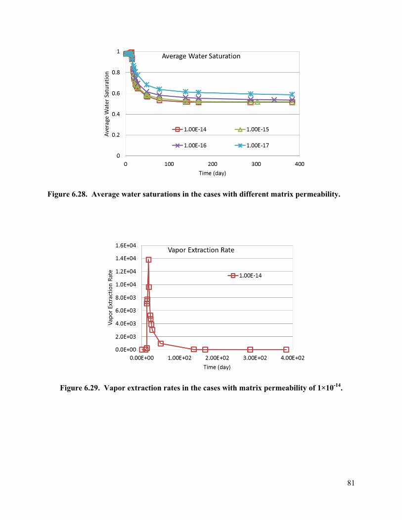
Figure 6.28. Average water saturations in the cases with different matrix permeability.

Figure 6.29. Vapor extraction rates in the cases with matrix permeability of 1×10-14.

81

Figure 6.30. Vapor extraction rates in the cases with matrix permeability of 1×10-15.

Figure 6.31. Vapor extraction rates in the cases with matrix permeability of 1×10-16.

82

Figure 6.32. Vapor extraction rates in the cases with matrix permeability of 1×10-17.

Figure 6.33. Fraction of initial 1,2-DCA mass in the cases with different matrix permeability.

83

6.3.6 Effect of Operational Strategies

Different operational strategies have been simulated to demonstrate the contaminant removal from fractured rock. Simulation results are shown in the Figure 6.34.

In the base case (case1), the model simulates treating a contaminated fractured site by heating and extracting for 18 days, followed by extracting for 365 days. There is 43.4% of 1,2-DCA mass removed after 18 days of heating and extraction. Further extraction for 365 days removes another 47.25% contaminant mass. At the end of the simulation, there is 9.35% mass that remains in the zone untreated (90.65% mass removal).

The second case (case2) simulates to heating the fractured site for a longer time- 23 days (with extraction during heating), followed by vapor extraction for 360 days. Compared to the case1, better contaminant removal is observed in this case. The heating and extraction period corresponds to the removal of 88.81% of the 1,2-DCA mass. Further extraction removes another 10.563% mass. After treatment, only 0.627% 1,2-DCA mass remains, for a removal efficiency of 99.37%.

Cycling is simulated in the third case (case3). In this case, the site is heated with extraction wells on for 18 days; then the heater is turned off leaving the extraction on for another 50 days; then heating is resumed for another 5 days (with extraction), followed by extracting for 310 days. Compared to the case2, the same amount of energy is consumed here. The first part of heating and extracting is the same as in the case2, and 43.4% 1,2-DCA is removed. The following extraction for 50 days (1st extraction) corresponds to a removal of another 44.7% of the 1,2-DCA mass. Further heating and extracting for 5 days (2nd heating & extracting) results in 2.33% 1,2-DCA removal. The last part of extracting removes another 9.39% 1,2-DCA mass. By the end of the simulation, this process removes 99.82% 1,2-DCA mass from the.

All the above strategies considered cases of heating the contaminated site with the extraction well on. However, the fourth case (case4) considers heating the site without extracting for 18 days, followed by extracting for 365 days. The same amount of energy is consumed as in the case1. Because there is no extraction during the heating period, no contaminant is removed in the first 18 days. After the heater is turned off and the extraction well is turned on, the 1,2-DCA mass is quickly removed from the fractured site. After extracting for 30 days (in day 48), 94.3% 1,2-DCA mass is removed. After 383 days, there is only 3.07% contaminant mass remaining, for an overall removal efficiency of 96.93%, which is better than in case 1.

Cycling is tested again in the fifth case (case5). The model simulates heating the site for 16 days without extraction, followed by extracting for 50 days, then heating for another 2 days without extraction, followed by extracting for 315 days. Because the extraction wells are off during heating, there is no contaminant removal in the first 16 days. Extracting for 50 days following the first heating period removes 83.1% of the 1,2-DCA mass. The second round of heating followed by extracting removes 8.18% 1,2-DCA mass. At the end of 383 days, 8.72% contaminant mass remains for a removal efficiency of 91.28%. Compared to the cases 1 and 4, the same amount of total energy for heating is consumed. In terms of contaminant removal, it is less effective than the strategy used in the case4, but slightly more effective than in the case1.

84

The previous simulations in the cases1 to 5 suggest that it is important to heat the zone to a high temperature before vapor is extracted. The sixth case (case6) models an extended heating period, where the heated site is heating for 23 days without extraction, followed by extraction for 365 days. The simulated results in the case6 show that a much improved contaminant removal is obtained when the treatment zone is heated to a higher temperature before vapor is extracted. In this case, due to no extraction during the heating, all the energy is used to increase the temperature of the subsurface. When the extraction well is turned on, a quick removal of 1,2-DCA is observed. Extraction for 30 days decreases the 1,2-DCA mass by more than 4 orders of magnitude. After 383 days, only 9.43×10-6 of the initial 1,2-DCA mass remains for a removal efficiency of 99.9991%. This is the most effective strategy that has been simulated here.

The seventh case (case7) investigates the performance of cycling heating and extraction when an increased amount of thermal energy is delivered. It simulates heating for 18 days without extraction, followed by extraction for 50 days, followed by heating for 5 days without extraction, and finally, extracting for 310 days. The total energy for heating is the same as in the cases 2, 3 and 6. From the Figure 6.34, the simulation results show that, although the same amount of thermal energy is consumed, this strategy is less effective than the case6 in terms of contaminant removal. After treatment for 383 days, it removes about 99.671% 1,2-DCA mass, leaving 0.329% of the 1,2-DCA mass untreated. It is less effective than the case3 where cycling is used and extraction wells are on while heating, but more effective than the case2 where no cycling is used. From the comparison of the cases 2, 3, and 7, with 6, we can conclude that for the same amount of thermal energy input, the best strategy appears to be to increase the formation temperature as much as possible, without extraction during heating. If the temperature cannot be allowed to increase too much, it is better to heat the formation in several cycles (e.g. cases 3 and 7 are better than the case 2). However, the comparison between the cases 3 and 7, shows that the case7 has a better removal rate than the case3 in the first round (e.g. After treatment of 68 days, 95.24% removed in the case7 while only 88.1% removed in the case3), but has a lower removal rate than the case3 in the second round (e.g. from days 69 to 383 days, 11.72% 1,2-DCA is removed in the case3 while only 4.431% is removed in the case7).

The case8 simulates treating the assumed site by heating for 18 days without extraction, followed by extraction for 50 days, then heating and extracting for 5 days, followed by extraction for 310 days. Different from the case 7, the extraction well is turned on in the second round of heating (from days 69 to 73). It seems that turning on the extraction well during the second round of heating improves the contaminant removal: 4.61% 1,2-DCA mass is removed from the days 69 to 383. At the end of treatment, only 0.15% 1,2-DCA remains, which is a little less than the remaining mass in the case3 (0.18% 1,2-DCA).

85

Figure 6.34 Contaminant removal efficiencies from different operational strategies.

As a summary, simulations of the contaminant removal with the different treatment strategies show that increased thermal energy input will increase the performance of thermal remediation. If the energy consumption is a concern, it is recommended to use as much of the energy as possible to increase the subsurface temperature, following by extraction. If for some reasons, the temperature cannot be too high, it is better to deliver the energy in several rounds. Extraction might be beneficial in the second round of heating.

86

6.4 References

Adenekan, A. E. 1992. Numerical modeling of multiphase transport of multicomponent organic contaminants and heat in the subsurfaceUniversity of California at Berkeley.

Adenekan A. E., Patzek TW, Pruess K, 1993. Modeling of multiphase transport of mulitcomponent organic contaminants and heat in the subsurface: numerical model formulation. Water Resour.Res. ;29(11):3727-40.

Chen F, Liu X, Falta RW, Murdoch LC, 2010. Experimental demonstration of contaminant removal from fractured rock by boiling. Environ.Sci.Technol. ;44:6437-42.

Falta RW, Pruess K, Finsterle S, Battistelli A, 1995. T2VOC user's guide. ;LBL-36400.

Falta RW, Pruess K, Javandel I, Witherspoon PA, 1992. Numerical modeling of steam injection for the removal of nonaqueous phase liquids from the subsurface 2. code validation and application. Water Resour.Res. ;28(2):451-65.

Gudbjerg J, Sonnenborg TO, Jensen KH, 2004. Remediation of NAPL below the water table by steam-induced heat conduction. J.Contam.Hydrol. ;72:207-25.

Ochs SO, Hodges RA, Falta RW, Kmetz TF, Kupar JJ, Brown NN, et al, 2003. Predicted heating patterns during steam flooding of coastal plain sediments at the Savannah River Site. Environmental and Engineering Geoscience ;9(1):51-69.

Pruess K, Battistelli A, 2002. TMVOC, A numerical simulator for three-phase non-isothermal flows of multicomponent hydrocarbon mixtures in saturated-unsaturated heterogeneous media. ;LBNL-49375.

Pruess K, 2002. Numerical simulation of multiphase tracer transport in fractured geothermal reservoirs. Geothermics ;31:475-99.

Pruess K, Narasimhan TN, 1985. A practical method for modeling fluid and heat flow in fractured porous media. Society of Petroleum Engineers Journal ;25(1):14-26.

Tse KKC, Liou T, Lo S, 2006. Numerical simulation of a steam-injection pilot study for a PCP-contaminated aquifer. Environ.Sci.Technol. ;40:4292-9.

van Genuchten MT, 1980. A closed-form equation for predicting the hydraulic conductivity of unsaturated soils. Soil Sci.Soc.Am.J. ;44:892-8.

87

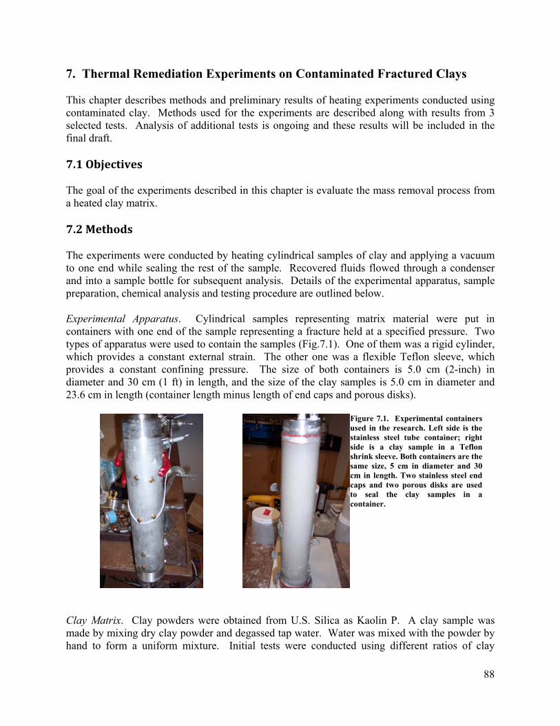
7. Thermal Remediation Experiments on Contaminated Fractured Clays

This chapter describes methods and preliminary results of heating experiments conducted using contaminated clay. Methods used for the experiments are described along with results from 3 selected tests. Analysis of additional tests is ongoing and these results will be included in the final draft.

7.1 Objectives

The goal of the experiments described in this chapter is evaluate the mass removal process from a heated clay matrix.

7.2 Methods

The experiments were conducted by heating cylindrical samples of clay and applying a vacuum to one end while sealing the rest of the sample. Recovered fluids flowed through a condenser and into a sample bottle for subsequent analysis. Details of the experimental apparatus, sample preparation, chemical analysis and testing procedure are outlined below.

Experimental Apparatus. Cylindrical samples representing matrix material were put in containers with one end of the sample representing a fracture held at a specified pressure. Two types of apparatus were used to contain the samples (Fig.7.1). One of them was a rigid cylinder, which provides a constant external strain. The other one was a flexible Teflon sleeve, which provides a constant confining pressure. The size of both containers is 5.0 cm (2-inch) in diameter and 30 cm (1 ft) in length, and the size of the clay samples is 5.0 cm in diameter and 23.6 cm in length (container length minus length of end caps and porous disks).

Figure 7.1. Experimental containers used in the research. Left side is the stainless steel tube container; right side is a clay sample in a Teflon shrink sleeve. Both containers are the same size, 5 cm in diameter and 30 cm in length. Two stainless steel end caps and two porous disks are used to seal the clay samples in a container.

Clay Matrix. Clay powders were obtained from U.S. Silica as Kaolin P. A clay sample was made by mixing dry clay powder and degassed tap water. Water was mixed with the powder by hand to form a uniform mixture. Initial tests were conducted using different ratios of clay

88

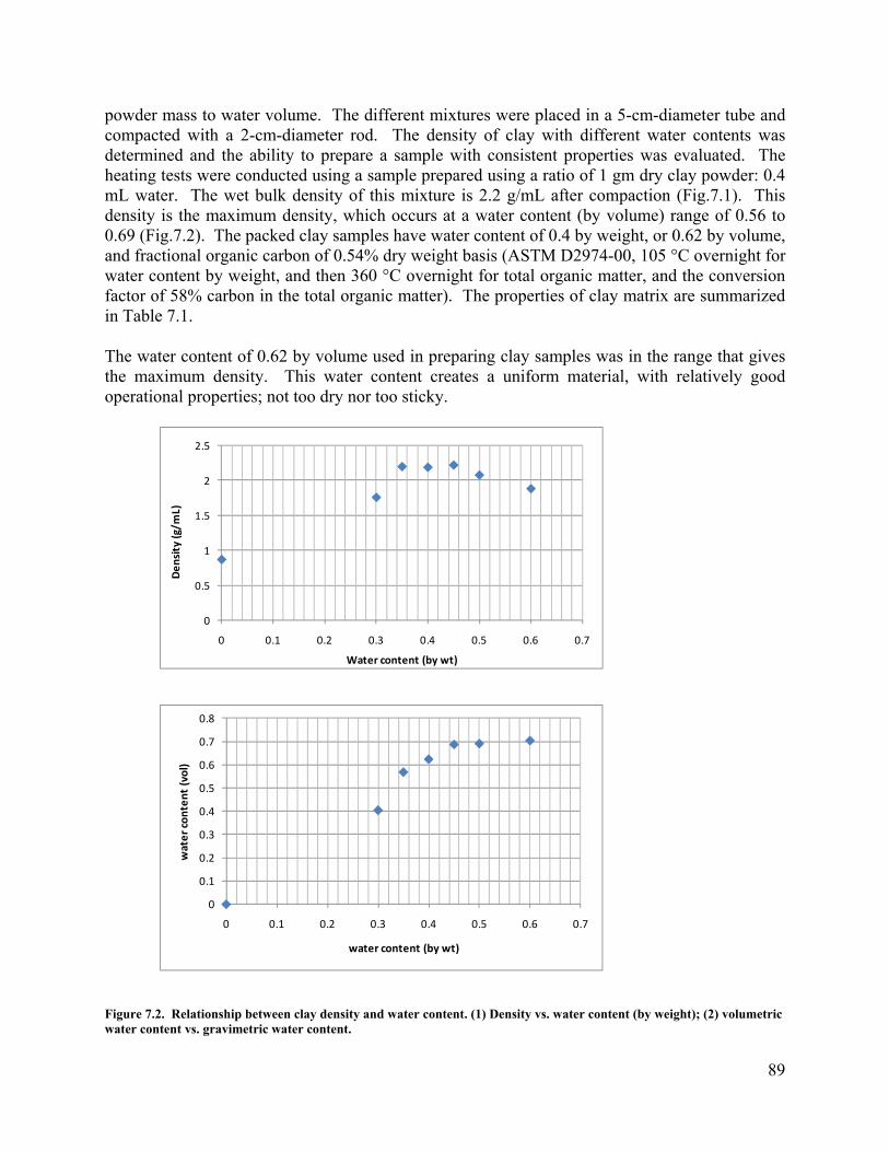
powder mass to water volume. The different mixtures were placed in a 5-cm-diameter tube and compacted with a 2-cm-diameter rod. The density of clay with different water contents was determined and the ability to prepare a sample with consistent properties was evaluated. The heating tests were conducted using a sample prepared using a ratio of 1 gm dry clay powder: 0.4 mL water. The wet bulk density of this mixture is 2.2 g/mL after compaction (Fig.7.1). This density is the maximum density, which occurs at a water content (by volume) range of 0.56 to 0.69 (Fig.7.2). The packed clay samples have water content of 0.4 by weight, or 0.62 by volume, and fractional organic carbon of 0.54% dry weight basis (ASTM D2974-00, 105 °C overnight for water content by weight, and then 360 °C overnight for total organic matter, and the conversion factor of 58% carbon in the total organic matter). The properties of clay matrix are summarized in Table 7.1.

The water content of 0.62 by volume used in preparing clay samples was in the range that gives the maximum density. This water content creates a uniform material, with relatively good operational properties; not too dry nor too sticky.

0

0.5

1

1.5

2

2.5

0 0.1 0.2 0.3 0.4 0.5 0.6 0.7

Den

sity (g/m

L)

Water content (by wt)

0

0.1

0.2

0.3

0.4

0.5

0.6

0.7

0.8

0 0.1 0.2 0.3 0.4 0.5 0.6 0.7

water co

nten

t (vol)

water content (by wt)

Figure 7.2. Relationship between clay density and water content. (1) Density vs. water content (by weight); (2) volumetric water content vs. gravimetric water content.

89

Table 7.1 Properties of clay

Bulk density (g/mL) 2.2 Sample dimensions 0.24 m long, 5 cm diameter

Water content (by volume) 0.62 Water: dry clay 0.4mL:1g Water content (by weight) 0.4 Organic carbon fraction (foc) 0.54% Water content (by volume)=water volume/sample volume Water content (by weight)=water weight/dry clay weight Water density=1 g/mL (to estimate water volume from water weight) Water loss is measured by oven dry clay sample at 105 °C for overnight

Samples were contaminated with a solution containing a dissolved volatile organic compound (VOC) and nonvolatile bromide. The solution was introduced by two methods, a.) point injection of aqueous solution into the packed sample; or b.) making the sample using water containing the VOC and bromide. For the latter method, the clay powder was measured in a glass tray and placed in an active fume hood. The well mixed solution of the VOC and bromide was added gradually to the powder. The mixture was manually kneaded into a uniform dough-like material that was divided into three parts. Each part was placed into a container (the stainless steel tube or the Teflon sleeve) that was sealed at the bottom by a stainless steel end cap. A 2.5-cm diameter metal rod was used to compact the clay as the container was filled. Another stainless steel end cap was placed at the top to seal the clay sample. This process took about 15-20 min to mix and knead the dough, another 15-20 min to pack the dough into the container and seal it. The sample weight was measured by the weight difference between the empty container and the packed container. The sample was allowed to equilibrate for >16 h (ASTM D698-07) before heating.

Clay samples were taken to measure the initial mass of the VOC in the packed clay. A plastic syringe with the end removed was used to take samples and measure their volume. The headspace extraction method was used based on USEPA method 5021A “Volatile organic compounds in various sample matrices using equilibrium headspace analysis.” Approximately 6-7 g of clay sample is placed in a screw-caped 40-mL vial with Teflon-faced septa containing 10 mL saturated sodium chloride solution (150 g NaCl in 500 mL de-ioned distilled water). The mixture was vigorously mixed using a vortex for 15 seconds and placed on an orbit shaker for more than 1 h at 115 rpm. The headspace of the samples was analyzed by gas chromatography equipped with flame ionization detector (GC-FID) to determine for VOC concentrations.

Concentrations of contaminants were measured both before and after the heating tests. The clay was quite dry and rigid after heating, so cm-sized fragments were broken loose and placed in a vial with a sodium chloride solution. The VOC concentrations after heating were lower than before heating, so headspace gases were analyzed using a GC equipped with electron capture detector (GC-ECD).

The method of extracting contaminants using the sodium chloride solution was evaluated by comparing results to those obtained using the methanol extraction method described by

90

Dincutoiu et al [2003]. The results were similar but the headspace extraction method using a sodium chloride solution takes much less time (1 h vs. 5 day).

Analytical Methods. A solution of 1,2-dichloroethane (DCA) and bromide was used to contaminate the samples. Gas chromatography (GC) was used to analyze the DCA, and ion chromatography (IC) was used to measure bromide concentration. DCA in the collected outflow condensate was analyzed by injecting headspace samples (500 µL) onto a HP 5890 Series II Plus GC equipped with an RTX 5 column (30-m x 0.53-mm x 1.5-µm film; Restek Corp.) and flame ionization detector (FID). The injector and detector temperatures were 250°C and 325°C, respectively. The oven temperature program was 50°C for 4 min, increased at 10°C/min to 80°C, and held 2 min. Helium (5 mL/min) was used as the carrier gas and nitrogen (30 mL/min) was the makeup gas [Elango, 2010]. The GC response to a headspace sample was calibrated to give the total mass of compound in that bottle and assuming the headspace and aqueous phases were in equilibrium [Gossett, 1987].

For solvent extraction method for clay samples, methanol (Burdick and Jackson) and hexane (Fisher Scientific) were HPLC grade. The methanol extract was exchanged into hexane to inject into GC-ECD [Dincutoiu et al., 2003]. Standards for methanol extraction were prepared for five levels of concentration of DCA with 1,2-dibromoethane (EDB) as the internal standard, from 0.63 to 1.24 mg/L (final concentrations of DCA in hexane). The hexane extract was analyzed by injecting 1 µL onto a Hewlett Packard 5890 Series II Plus GC equipped with an HP 7673 autosampler, ZB 624 capillary column (30 m x 0.53 mm x 3.0 µm film; Zebron) and electron capture detector (ECD). A single temperature program (40°C for 5 min, ramped at 10°C/min to 200°C, hold for 2 min) resolved DCA and EDB, with injector and detector temperatures set at 200°C and 260°C, respectively. Elution times for DCA and EDB were 13.2 and 17.0 min, respectively. Helium (3 mL/min) and nitrogen (33 mL/min) served as the carrier and make-up gases, respectively [Henderson, 2008]. For low concentration headspace extraction samples as well as low concentration aqueous samples, the same ECD program was used except the autosampling was changed to manual injection of 0.5 mL gas phase samples. For aqueous samples, standards were prepared for six to ten levels of concentration, from 0.16 to 909.0 mg/L for GC-FID and 0.0086 to 0.34 mg/L for GC-ECD for manual injection of headspace of 0.5 mL gas phase. For headspace extraction samples, standards were prepared for six levels of concentration: 2.9 to 68.6 μg DCA/g clay (wet) on GC-FID, and 0.095 to 0.96 μg DCA/g clay (dry) on GC-ECD.

Bromide was measured on a Dionex AS50 ion chromatography system equipped with a CD25 conductivity detector and a Dionex guard column (AG14, 4 mm×50 mm) followed by an IonPac® AS14 anion-exchange column (4 mm×250 mm). Eluant (4.5 mM Na2CO3 and 0.8 mM NaHCO3) was delivered at 1.0 mL/min. Six-point standards were prepared from 0.10 to 116.24 mg/L as bromide.

91

Figure 7.3. The experimental apparatus: The flexible-wall Teflon shrink tube contained sample is in a pressure chamber on the left, and the rigid-wall stainless steel tube contained sample stands on the right. The top outlet tubing is connected to the copper heat exchanger. The other end of the heat exchanger is a needle (not shown) to be inserted into a pre-sealed pre-vacuumed bottle for sample collection.

Heating Test. The packed clay column, in either a stainless steel tube or a Teflon shrink sleeve, was sealed at the two ends with stainless steel end caps with Teflon coated o-rings. The column was placed vertically with flow from bottom to top and the outlet tubing extended from the center of the upper end cap through the condenser and then to a sample bottle (Fig.3). The packed clay column was wrapped with heating tape (SRT051-120, Omega, U.S.) on the entire surface and there were also cartridge heaters embedded in the two end caps. Micro-thermistors (10K3MCD1, Measurement Specialties, US) were inserted into the center of the sample along the column length to monitor temperatures, and resistivity temperature device (RTD) probes (SA1, Omega, US) were attached on the surface of the column.

After the matrix was heated to above 100 ºC shown by all the thermistors and RTD, the outlet valve was opened. This caused flow out of the sample, through the condenser and into a 50 mL glass vial sealed with screw-cap and Teflon faced septa. Each vial was sealed and pre-vacuumed by removing 10 mL of air to accommodate 10 mL condensate. When ~10mL of condensate accumulated in the vial, the outlet valve was closed and the vial was removed and replaced with an empty one. Vials were weighed before and after collection of the condensate. The outflow

92

mass was recorded over time, and DCA in the outflow was measured by GC-FID. After GC measurement the condensate samples were filtered with a 0.45 μm syringe filter and bromide concentration was measured with an IC. The mass recovery was obtained by integration of the collected outflow volume and the concentrations of DCA and bromide.

7.3 Results

The testing program consists of approximately ten tests conducted on clay materials. Three tests were selected for presentation here to demonstrate typical behaviors (Table 7.2). The first test presented below is a clean clay matrix contaminated by point injection at the bottom side (far end from the outlet) in the rigid-wall stainless steel column. The next one is a clean clay matrix contaminated by point injection at the flexible-wall Teflon shrink tube. The third one is a clay matrix uniformly contaminated by using DCA-laden water and packed in the rigid-wall stainless steel column.

Table 7.2 Summary of three tests of heating clay matrix

Test Container type

Contamination type

Cinjection DCA/Br (mg/L); or C0 for working solution to make the dough

Max. Cout/Cinjection or Cout/C0 for DCA

Mass recovery (Mout/Min) for DCA and Bromide

Heating for tape heater (duty cycle×Power)

Total water boiled out/pore volume

Heating time to boil out the pore water (h)

1 Constant external strain (rigid-wall)

Point injection 1.7 mL (high concentration)

1058/ 33939

6% 63%/7.5% 0.1×313W 94% 84 (open outlet @ t=6.25 h)

2 Constant confining pressure (flexible-wall)

Point injection 2 mL (low concentration)

191/75 1% 38%/37% 0.13×313W 91% 119 (open outlet @ t=2.9 h)

3 Constant external strain (rigid-wall)

uniform 147/520 297% 90%/1% 0.5×313W 104% 6.6 (open outlet @ t=1.3 hr)

Test 1: Sample in rigid tube, point injection of contaminant

Set up: 1.7 mL DCA-Bromide solution was injected at a point along the sample; the concentration of DCA was measured by GC-FID to be 1058 mg/L, and bromide was measured on IC to be 33939 mg/L (a ~1/300 dilution factor was used to make the concentration to fall into the calibration range).

93

Results

The outflow is characterized by a sharp pulse of relatively rapid flow followed by a period of roughly constant flow until the sample is dry (Fig.7.4a). The initial outflow pulse starts as soon as the valve is opened (at t=6.25 h), reaching a maximum flow of 44 mL/hr (Fig.4a and 4c). After the initial pulse is over, the flow drops to between 1 and 10 mL/hr and is maintained for approximately 80 hrs, with an exception of between hr 35 and 47 when the flow was dropped to about 1 mL/hr because the heating program was shut down inadvertently. The outflow rate is nearly constant at 4.0 mL/hr before and after the period of low flow. The experiment produced a total of 255 mL of water, or 94% of the estimated pore volume of the clay matrix (270 mL).

The concentration of DCA in the outflow increased rapidly at the beginning of the test and then dropped (Fig.7.4b). It reached a maximum value of 5.6% of the concentration in the injection solution at 6.93 h (Fig.4d). This concentration was maintained for 16 minutes (6.93 h-7.2 h) (Fig.4d) and then the concentration decreased to approximately 1% of the input at t=10 h. This resulted in two distinct stages of mass recovery rate, an initial rapid stage (t=6.25 h-7.93 h) followed by a second stage of lower rate (t=7.93 h-18.3 h) (Fig.4d). The average mass recovery rate during Stage I was approximately 582 μg/hr, and it dropped to 31 μg/hr during the Stage II.

The total mass of recovered DCA increased roughly linearly during the first and second recovery stages with the two different recovery rates, reaching a maximum recovery of approximately 74% of the initial injected mass. Roughly 2/3 of the recovered mass was achieved during Stage I when the rate was highest. Stage I occurs during the initial large rate of volumetric outflow, but the total amount of water produced during this time is a relatively modest 30 mL, which is 0.1 of the total water volume. The second stage of recovery was responsible for approximately 1/3 of the recovered mass and it produced approximately 220 mL of the total water volume, but at a slower rate than during the first stage. All the mass recovered during the test was produced during the first 20 hrs when 85 mL or less than 1/3 of the water was removed from the sample.

The bromide concentration in the outflow was consistently less than 1% of the injected concentration (Fig. 7.4b). A total of 7.5% of the total mass of injected bromide was recovered.

Temperatures increased as the sample was heated at constant power input. Most of the temperatures were within a 4°C band, except the temperature of the lower end cap, which was significantly hotter (Fig. 7.4c). A separate heater provided more power to the lower end cap than the rest of the sample and that is why it heated faster. The valve was opened at t=6.25 hrs when all the temperatures reached or exceeded 100°C. In general, thermistors at the top of the sample were cooler (~100°C) than those at the bottom of the sample (~104°C) early in the test (Fig. 7.4c).

Temperatures dropped sharply when the valve was opened. This apparently occurred as a result of the decrease in pressure, which lowered the boiling temperature. Nearly all of the temperatures dropped when the valve was initially opened, but there was an exception at sensors 11 and 12, where the temperature remained unaffected when the valve was initially opened.

94

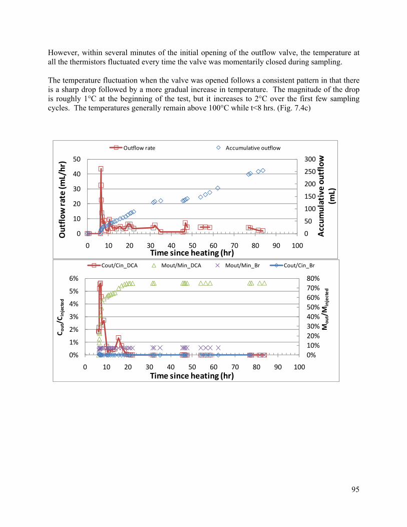
However, within several minutes of the initial opening of the outflow valve, the temperature at all the thermistors fluctuated every time the valve was momentarily closed during sampling.

The temperature fluctuation when the valve was opened follows a consistent pattern in that there is a sharp drop followed by a more gradual increase in temperature. The magnitude of the drop is roughly 1°C at the beginning of the test, but it increases to 2°C over the first few sampling cycles. The temperatures generally remain above 100°C while t<8 hrs. (Fig. 7.4c)

0

50

100

150

200

250

300

0

10

20

30

40

50

0 10 20 30 40 50 60 70 80 90 100

Accum

ulative ou

tflow

(mL)

Outflow

rate (m

L/hr)

Time since heating (hr)

Outflow rate Accumulative outflow

0%10%20%30%40%50%60%70%80%

0%

1%

2%

3%

4%

5%

6%

0 10 20 30 40 50 60 70 80 90 100

Mou

t/M

injected

C out/C

injected

Time since heating (hr)

Cout/Cin_DCA Mout/Min_DCA Mout/Min_Br Cout/Cin_Br

95

0

50

100

150

200

250

300

05101520253035404550

0 10 20 30 40

Accum

ulative ou

tflow (m

L)

Outflo

w rate (m

L/hr)

Time since heating (hr)

Outflow rate Accumulative outflow

0%

10%

20%

30%

40%

50%

60%

70%

80%

0%

1%

2%

3%

4%

5%

6%

0 10 20 30 40

DCA

_Mout/M

injected

DCA

_Cout/C injected

Time since heating (hr)

Cout/Cin Mout/Min(c)

Stage I Stage II

96

Figure 7.4. Heating test of a clay matrix contained in a rigid tube. . (a) Condensed outflow rate in mL/h and accumulative outflow in mL during heating, (b) DCA and bromide concentrations in the outflow, normalized to the injection concentration, 1058 mg/L and 33939 mg/L, respectively, and DCA and bromide mass recovery, normalized to the injected mass, 1799 μg and 57696 μg, respectively, during heating, (c) Scaled up condensed outflow rate and accumulative outflow during heating for the first 35 hr and dashed line is the divide of Stage I and Stage II, (d) Scaled up normalized DCA concentrations in outflow and mass recovery during heating for the first 35 hr and solid lines to dashed line are Stage I and Stage II, and (e) temperature time series at different locations during heating.

The power to the heaters was inadvertently turned off by the control system at t~8 hrs, and this caused all the temperatures to decrease below 100°C. The power was restored at t = 8.5 hrs, and the temperatures increased to above 100°C and then they cycled over several degrees with a mean of roughly 100°C (Fig. 7.4c).

All the temperatures cycled during each sampling event, but the magnitude and shape of the response depends on the location. In general, the magnitude of the temperature response was greatest at the top of the sample and became progressively less with distance below the top. The transitions in temperature were sharp near the top of the sample, but became progressively more gradual with distance from the top. An exception occurred at thermistor 10, which was in the middle of the sample and was consistently hotter than the others. (Fig. 4c)

The change in magnitude and shape that occurred as a function of distance from the end of the sample is evident from hours 10 to 15. The differences in temperature response gradually

97

diminished, however, and by t= 20 hours the shapes of the temperature time series are essentially identical. (Fig. 7.4c)

A temperature gradient occurs along the length of the core during each fluid sampling event. The temperature gradient reaches a maximum value when the temperatures reach a minimum, which occurs immediately before a new sample bottle is installed. The temperature gradient is approximately 0.1 oC/cm during hours 6<t<7 (the first hour after the valve was opened), it decreases to 0.05 oC/cm during hours 10<t<15, and it is essentially maintained at this value during t>20hrs. (Fig.7. 4c)

Test 2: Sample in flexible sleeve, point injection of contaminant.

Set up: 2 mL DCA-bromide solution was injected at a point 20 cm from the end cap, DCA: 191.4 mg/L; bromide: 74.8 mg/L.

Results

Condensate was produced at a flow in range of 6 to 12 mL/hr during the first 20 hrs (Fig. 5a). The outflow then dropped abruptly to 3 mL/hr at t=20 hrs, and it tapered to negligible rates over the next 80 hrs.

Both the first and second test produced about the same amount of water, and they both are characterized by a relatively large initial flow rate that decreases with time. However, compared to the first test, the flow rate from the flexible sleeve was slower at first because it lacked the large initial outflow pulse that occurred from the rigid wall container. However, the flowrate from the rigid wall dropped off quickly, and after an hour the flow rate from the flexible sleeve was greater. Later in the test, when t>20 hrs, the flowrate from both devices was in the range of a few mL/hr.

Recovery of DCA during Test 2 increased and decreased as roughly a symmetric pulse, with a peak magnitude of 2% of the injected concentration and a duration of approximately 15 hours (Figure 5b). Small DCA concentrations were detectable almost immediately after opening the valve, and they increased gradually over the first few hours until reaching a peak at t=12 hrs. DCA concentration decreased gradually and were negligible when t> 20 hrs.

The style of recovery of DCA during Test 2 is much different than Test 1. The majority of DCA was recovered in a rapid surge within a fraction of an hour after the valve was opened during the first test, and then the rate tapered off for the next 10 hours. In contrast, during the

98

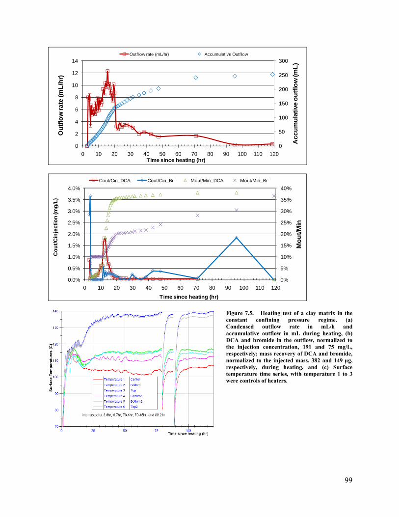
Figure 7.5. Heating test of a clay matrix in the constant confining pressure regime. (a) Condensed outflow rate in mL/h and accumulative outflow in mL during heating, (b) DCA and bromide in the outflow, normalized to the injection concentration, 191 and 75 mg/L, respectively; mass recovery of DCA and bromide, normalized to the injected mass, 382 and 149 μg, respectively, during heating, and (c) Surface temperature time series, with temperature 1 to 3 were controls of heaters.

0

50

100

150

200

250

300

0

2

4

6

8

10

12

14

0 10 20 30 40 50 60 70 80 90 100 110 120

Acc

umul

ativ

e ou

tflow

(mL)

Out

flow

rate

(mL/

hr)

Time since heating (hr)

Outf low rate (mL/hr) Accumulative Outf low

0%

5%

10%

15%

20%

25%

30%

35%

40%

0.0%

0.5%

1.0%

1.5%

2.0%

2.5%

3.0%

3.5%

4.0%

0 10 20 30 40 50 60 70 80 90 100 110 120

Mou

t/Min

Cou

t/Cin

ject

ion

(mg/

L)

Time since heating (hr)

Cout/Cin_DCA Cout/Cin_Br Mout/Min_DCA Mout/Min_Br

99

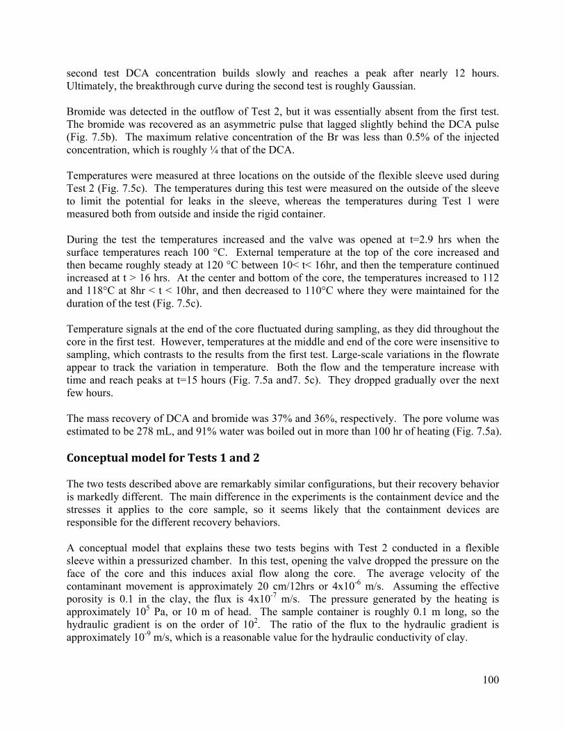
second test DCA concentration builds slowly and reaches a peak after nearly 12 hours. Ultimately, the breakthrough curve during the second test is roughly Gaussian.

Bromide was detected in the outflow of Test 2, but it was essentially absent from the first test. The bromide was recovered as an asymmetric pulse that lagged slightly behind the DCA pulse (Fig. 7.5b). The maximum relative concentration of the Br was less than 0.5% of the injected concentration, which is roughly ¼ that of the DCA.

Temperatures were measured at three locations on the outside of the flexible sleeve used during Test 2 (Fig. 7.5c). The temperatures during this test were measured on the outside of the sleeve to limit the potential for leaks in the sleeve, whereas the temperatures during Test 1 were measured both from outside and inside the rigid container.

During the test the temperatures increased and the valve was opened at t=2.9 hrs when the surface temperatures reach 100 °C. External temperature at the top of the core increased and then became roughly steady at 120 °C between 10< t< 16hr, and then the temperature continued increased at t > 16 hrs. At the center and bottom of the core, the temperatures increased to 112 and 118°C at 8hr < t < 10hr, and then decreased to 110°C where they were maintained for the duration of the test (Fig. 7.5c).

Temperature signals at the end of the core fluctuated during sampling, as they did throughout the core in the first test. However, temperatures at the middle and end of the core were insensitive to sampling, which contrasts to the results from the first test. Large-scale variations in the flowrate appear to track the variation in temperature. Both the flow and the temperature increase with time and reach peaks at t=15 hours (Fig. 7.5a and7. 5c). They dropped gradually over the next few hours.

The mass recovery of DCA and bromide was 37% and 36%, respectively. The pore volume was estimated to be 278 mL, and 91% water was boiled out in more than 100 hr of heating (Fig. 7.5a).

Conceptual model for Tests 1 and 2

The two tests described above are remarkably similar configurations, but their recovery behavior is markedly different. The main difference in the experiments is the containment device and the stresses it applies to the core sample, so it seems likely that the containment devices are responsible for the different recovery behaviors.

A conceptual model that explains these two tests begins with Test 2 conducted in a flexible sleeve within a pressurized chamber. In this test, opening the valve dropped the pressure on the face of the core and this induces axial flow along the core. The average velocity of the contaminant movement is approximately 20 cm/12hrs or 4x10-6 m/s. Assuming the effective porosity is 0.1 in the clay, the flux is 4x10-7 m/s. The pressure generated by the heating is approximately 105 Pa, or 10 m of head. The sample container is roughly 0.1 m long, so the hydraulic gradient is on the order of 102. The ratio of the flux to the hydraulic gradient is approximately 10-9 m/s, which is a reasonable value for the hydraulic conductivity of clay.

100

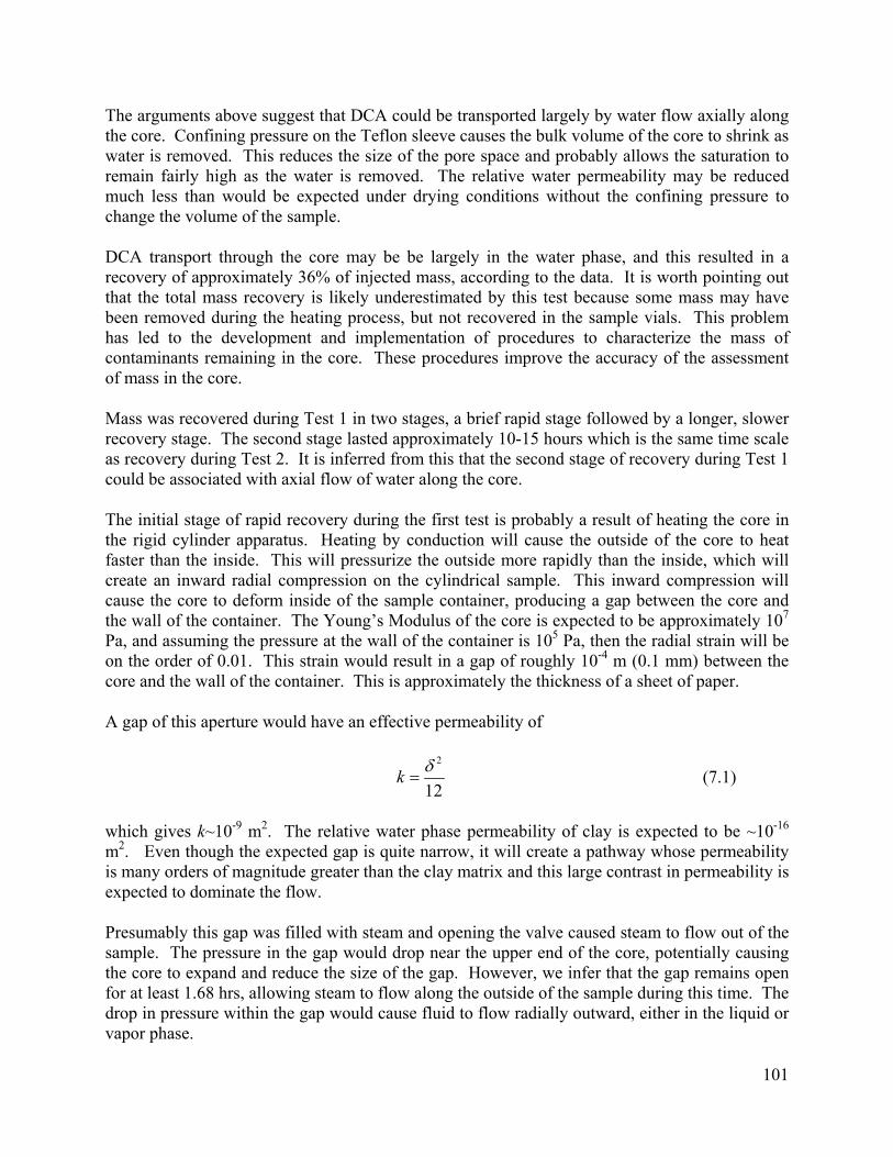
The arguments above suggest that DCA could be transported largely by water flow axially along the core. Confining pressure on the Teflon sleeve causes the bulk volume of the core to shrink as water is removed. This reduces the size of the pore space and probably allows the saturation to remain fairly high as the water is removed. The relative water permeability may be reduced much less than would be expected under drying conditions without the confining pressure to change the volume of the sample.

DCA transport through the core may be be largely in the water phase, and this resulted in a recovery of approximately 36% of injected mass, according to the data. It is worth pointing out that the total mass recovery is likely underestimated by this test because some mass may have been removed during the heating process, but not recovered in the sample vials. This problem has led to the development and implementation of procedures to characterize the mass of contaminants remaining in the core. These procedures improve the accuracy of the assessment of mass in the core.

Mass was recovered during Test 1 in two stages, a brief rapid stage followed by a longer, slower recovery stage. The second stage lasted approximately 10-15 hours which is the same time scale as recovery during Test 2. It is inferred from this that the second stage of recovery during Test 1 could be associated with axial flow of water along the core.

The initial stage of rapid recovery during the first test is probably a result of heating the core in the rigid cylinder apparatus. Heating by conduction will cause the outside of the core to heat faster than the inside. This will pressurize the outside more rapidly than the inside, which will create an inward radial compression on the cylindrical sample. This inward compression will cause the core to deform inside of the sample container, producing a gap between the core and the wall of the container. The Young’s Modulus of the core is expected to be approximately 107 Pa, and assuming the pressure at the wall of the container is 105 Pa, then the radial strain will be on the order of 0.01. This strain would result in a gap of roughly 10-4 m (0.1 mm) between the core and the wall of the container. This is approximately the thickness of a sheet of paper.

A gap of this aperture would have an effective permeability of

2

12k δ= (7.1)

which gives k~10-9 m2. The relative water phase permeability of clay is expected to be ~10-16 m2. Even though the expected gap is quite narrow, it will create a pathway whose permeability is many orders of magnitude greater than the clay matrix and this large contrast in permeability is expected to dominate the flow.

Presumably this gap was filled with steam and opening the valve caused steam to flow out of the sample. The pressure in the gap would drop near the upper end of the core, potentially causing the core to expand and reduce the size of the gap. However, we infer that the gap remains open for at least 1.68 hrs, allowing steam to flow along the outside of the sample during this time. The drop in pressure within the gap would cause fluid to flow radially outward, either in the liquid or vapor phase.

101

We infer that DCA was transported radially outward to the vapor-filled gap where it was transported axially and out of the container relatively rapidly. This process occurred during the first 16 minutes after the valve was opened and was dominated by vapor transport. This process is inferred to be responsible for the relatively rapid mass flux during the first stage of recovery of Test 1.

The process that shuts down Stage 1 is unclear, but it could be that the radial temperature gradient is diminished by conduction, which reduces the radial pressure gradient and causes the sample to expand and close the gap.

The first stage of recovery appears to be relatively brief, 1-2 h, and it is followed by axial flow that occurs on the same time scale as axial flow during Test 2. The temperature gradient during sampling progressively flattens during the test and this is inferred to be evidence for axial flow. The temperature gradient would produce a pressure gradient that would cause axial flow. If the mechanism of radial flow and then axial flow through a gap was active at this time then the core would change uniformly. The disassembled core after heating showed a roughly uniformly shrunk dry core with a gap between the container wall and the core.

This conceptual model is further supported by the record of bromide recovery, which is an indicator of the relative ratio of steam and water flowing from the core. Roughly the same fractions of bromide and DCA were recovered during Test 2, which suggests that these compounds were dissolved in water when they flowed out of the clay sample. In contrast, negligible amounts of bromide were produced with DCA during Test 1, which suggests that DCA was recovered in the vapor phase.

Test 3: Sample in rigid vessel, initial contaminant distribution uniform.

Clay mixed with water containing DCA and bromide was packed in the rigid wall container. This test differs from the other two in that all the clay was contaminated. The power used during Test 3 was approximately 5x greater than during Tests 1 and 2.

Results:

This test required more extensive sampling and analysis than the point injection tests to characterize the initial mass of contaminants. The clay was sampled to measure DCA concentration in the solids before and after the heating test using two extraction methods; the headspace extraction with sodium chloride solution, and the methanol extraction. Average DCA concentration before heating measured with headspace extraction was 10.75 ±1.40 µg DCA/g clay (n=4). A duplicate clay sample made with the same working solution was measured to be 10.29±1.60 µg DCA/g clay (n=4). These two results suggest that the headspace method is repeatable. Methanol extraction had a slightly lower mean and more variable result, 9.31±2.20 µg DCA/g clay (n=4), although the difference between the means is not statistically significant.

The mass in the clay before heating was calculated as 10.75 µg DCA/g clay times the weight of clay, 791.9 g, to get 8513.5 µg DCA. Water content of the clay sample before heating (water weight/dry clay weight) is 42.1% ±0.3% (wt) (n=5).

102

Table 7.3. Summary of Test 3 Headspace

extraction (µg DCA/g clay as is)

Methanol extraction (µg DCA/g clay)

Water content (by weight)

Headspace extraction (µg DCA/g clay_dry basis)

Before heating 10.75 ±1.40 9.31±2.20 42.1%±0.3% 15.27 After heating 0.174±0.013 0.074±0.048 1.0%±0.2% 0.176 Mass removal rate from clay (dry basis): 98.8%

The headspace extraction gave 0.174±0.013 μg DCA/g clay (dry) (n=5), whereas the methanol extraction had 0.074±0.048 μg DCA/g clay (dry) (n=5). Water content of the dry clay after heating (water weight/dry clay weight) is 1.0% ±0.2% (wt) (n=5). The remaining DCA in the clay estimated using the 0.174 μg DCA/g clay (dry) is 1.1% of the total mass inside the clay before heating, results using concentrations from the methanol extraction were less than half this value.

As in Test 1, the outflow in Test 3 is characterized by a sharp pulse of relatively rapid flow followed by a gradual decrease in flow until the sample is dry (Fig.6a). The initial pulse starts as soon as the valve is opened (at t=1.3 hr) and lasts for approximately 16 minutes, reaching a maximum flow of 326 mL/hr in less than 10 min after the valve is opened. After the initial pulse is over, the flow drops from 70 to 7 mL/hr in 5 hrs. The experiment produced a total of 244 mL of water, or 104% of the estimated pore volume of the clay matrix (234 mL).

The concentration of DCA and bromide were normalized to the working solution used to make the clay sample (147.0 mg/L for DCA and 519.5 mg/L for bromide). The total mass of recovered DCA occurred in the first 10 min and then dropped to nearly zero. The total fraction of recovered DCA is 0.9, and this occurred after 70 mL, or 0.3 of the estimated pore volume. The bromide level, in contrast, was consistently low during the entire recovery (Fig.7.6b), indicating that the outflow was from condensed water vapor.

The core temperatures along the axis of the column were nearly identical during recovery (Fig. 7.6c and 7.6d). There was a slight variation in temperature during the first few sampling events, but then all the temperatures were within the line thickness (fraction of °C) during the remainder of the test. The temperatures oscillated during sampling, from 97.5 to 102.5 °C, which is the typical response from the other tests.

The temperature rose from 100 °C to the set point of the heater, 150 °C, in a sequence from the outlet downward. The temperature increase is inferred to mean that the clay was dry and latent heat of vaporization was negligible at that location. The sequential increase in temperature indicates that the clay dried from the top down (Fig.7.6c).

The pressure along the length of the core was measured by attaching transducers to ports tapped into the side of the sample container. The pressures were approximately 69 kPa (10 psi) before

103

the valve was opened, and then they oscillated and dropped when the first few samples were taken. The average pressure was atmospheric for t>1.8 hrs. The pressure oscillated when each sample was taken, with pressures dropping below atmospheric when the pre-vacuumed sample bottle was attached, and then rising as the sample bottle filled. The pressure change during sampling followed a remarkably consistent pattern during the test at each measurement location, but it differed markedly between the locations. The magnitude of pressure change during sampling increased from the top to the bottom of the sample. The pressure at the outlet of the core only varied a small fraction of 7 kPa (a psi) when each sample was taken, but the total variation was 7-14 kPa (1-2 psi) at mid-length, and 48-62 kPa (7-9 psi) near the bottom of the core.

The clay was dried to a hard, dry cylinder cut by several large fractures and many small ones. The diameter of the cylinder was approximately 4.95 cm (from an initial diameter of 5.08 cm), indicating a volumetric strain of approximately 0.05. The annular gap present at the end of the test was more than 1 mm wide. Through-going fractures cut the cylinder normal to its axis into several pieces 5 cm to 10 cm long, but continuous axial fractures were absent.

0%10%20%30%40%50%60%70%80%90%100%

0%

50%

100%

150%

200%

250%

300%

350%

0 1 2 3 4 5 6 7

Mou

t/Min

Cou

t/Cin

Time since heating (hr)

Cout/Cin_DCA Cout/Cin_Br Mout/Min_DCA Mout/Min_Br

0

50

100

150

200

250

0

50

100

150

200

250

300

350

0 1 2 3 4 5 6 7

Accu

mul

ativ

e ou

tflow

(mL)

Out

flow

rate

(mL/

hr)

Time since heating (hr)

Outf low rate Accumulative outf low

104

(c)

(d)

Figure 7.6. Heating test of a clay matrix of uniform contamination in a rigid wall container. (a) Condensed outflow rate in mL/h and accumulative outflow in mL during heating, (b) DCA and bromide in the outflow, normalized to the concentration of working solution to make the dough, i.e. C0, and DCA and bromide mass recovery during heating, normalized to the inside mass, measured by extraction of clay dough samples, (c) Core temperature time series during heating, and (d) Core temperature (expanded axis) and core pressure time series during heating. Fluctuations correlate with changing the sample bottle.

105

Discussion

The conceptual model outlined above is consistent with the results of Test 3. We suspect that the relatively large power used during Test 3 created a radial temperature gradient, which caused a radial pressure gradient that compressed the sample. This is the same process that occurred during Test 1, but it was amplified because of the larger power used during Test 3. As a result, we suspect that an annular space existed around the sample during Test 3 and this caused a rapid flow of steam and stripping of the DCA early in the test. It also reduced the pressure gradients along the core, and this homogenized the axial temperature profile.

Mass Balance

The mass balance on Test 3 was closed to within 10% (90% recovered and 1% remaining in the sample), which is within the expected tolerance for the experiments. A lower percentage of mass was recovered during the other two tests (30%-40%), but those two tests were conducted before the technique of measuring contaminants in the clay was developed. As a result, the fate of the mass that was not recovered could not be established.

We suspect that the mass remaining in the clay during the previous tests was low and similar to that measured in Test 3. The explanation is that mass was lost from the sample vessel during testing. This could occur by a small gas leak or by diffusion through seals, for example. We tested the fittings prior to each experiment by pressurizing the sample chamber with air. A few small leaks were detected using this procedure (the vast majority of the fittings never leaked), but it was impossible to test the fittings after the testing apparatus was filled with clay so it is possible that small leaks went undetected. It is also possible that DCA diffused out through the o-ring seals in the end caps and side fittings. We used Teflon-coated Viton o-rings in the end caps and silicone o-rings for the micro temperature sensors. These seals were selected because they can withstand elevated temperatures. The Teflon-coated Viton o-rings were used because they are particularly chemically inert. Silicone is less inert than Teflon-coated Viton, so it is possible that some mass was lost by diffusion through the silicone o-rings. We recognized this possibility, but silicone was the best available material for the small o-rings required to seal the temperature sensors—these o-rings were not available in Teflon-coated Viton.

The power used during Test 3 was roughly 5x greater than the power used during Test 1 and this caused the test to be completed in roughly 1/5 the time. If mass was lost from the sample container then reducing the time of the experiment would reduce the loss due to leakage. This may be one reason why the mass recovery from Test 3 was greater than from Test 1.

The leakage hypothesis may explain the low mass recovery during Test 2, but it is less likely than during the other tests. The clay in Test 2 was contained in a flexible Teflon membrane within a pressurized vessel. The pressure in the vessel was greater than the pressure in the sample, so flow out of the sample would have been prevented by this pressure difference. It is possible that DCA diffused through the Teflon membrane used in Test 2, but this seems unlikely because other tests with a larger fraction of mass recovery were conducted using the Teflon membrane.

106

Temperature variations

The variations in temperature and pressure are apparently inconsistent. Variations in temperature during sampling are nearly independent of location along the core during Test 3. Temperature is assumed to be a function of pressure in this system, so the similarity in the temperature records implies that the pressure is uniform. However, direct pressure measurements vary markedly along the core. A potential explanation for this is because the thermistors and pressure transducers measure different regions. The thermistors are embedded at the center of the sample, whereas the pressure transducers measure at the wall of the sample container.

We expect that the pressure within the sample varied at least as much as that indicated by the pressure record from 24 cm (bottom of the sample). The pressure variations at this transducer are closely correlated with the temperature variations. The temperature at this location varied by ~ 5oC and the pressure changed by 55 kPa to 69 kPa (8 psi to 10 psi) each time a sample was taken.

We assume that the pressure in the sample container at temperature T will follow the Clausius-Clapyron relation

1 1vap

o

HR T T

oP P eΔ ⎛ ⎞

− −⎜ ⎟⎝ ⎠= (7.2)

where Po is a reference pressure at the reference temperature To, and Hvap is the heat of vaporization. It follows that the sensitivity of pressure to temperature can be estimated at the boiling point under atmospheric pressure as

2373

3.4atm vapo

P HdP kPadT T R K

Δ= ≈ (7.3)

assuming Patm=101325 Pa (14.7 psi), T373 = 373oK, ΔHvap = 40 KJ mol-1, R = 8.3 J mol-1 K-1. This result is confirmed by using (equation 2) to calculate the pressure change from 97.5 to 102.5oC as 18.6 kPa (2.7 psi).

The temperature observed during sampling in all the thermistors ranges 97.5 to 102.5oC. According to the analyses outlined above, this should produce a change in pressure of 18.6 kPa (2.7 psi). This change in pressure was observed at the transducer at 9 cm below and at 31 cm above the outlet (Fig. 6d). However, the pressure varies by roughly 69 kPa (10 psi) at the transducer 24 cm below the outlet, and this variation is 4x greater than what can be explained from the temperature variations.

107

7.4 Summary

The results of heating tests show that volatile contaminants can be strongly removed from clay using heating, but the details of the process are sensitive to the design of the experiment. Tests conducted with clay inside a flexible Teflon membrane in a pressurized vessel (Test 2) appear to be characterized by flow along the axis of the sample. This is the intended flow geometry. Travel times along the axis of the core are consistent with transport in the water phase, and the presence of bromide in the outflow is also consistent with transport in water. However, DCA was recovered much more quickly than water. In all the experiments, all the DCA that could be recovered was produced when less 1/3 to 1/2 of the water in the clay was recovered, and this is an indicator of preferential transport in the vapor phase. It seems likely that transport occurred in both liquid and vapor phases during Test 2, but numerical transport analyses will be required to more fully evaluate this experiment.

The relatively low fraction of mass recovered in Test 2 may underestimate the fraction that could be recovered in the field. This is because mass may have been removed by the heating process, but not recovered in sample bottles; for example, if it diffused through seals. The recently developed technique of characterizing mass remaining in the sample will allow tests using the flexible Teflon membrane to be more accurately evaluated (this technique was unavailable when Test 2 was conducted).

The fraction of recovered mass during the experiments was variable, and may have resulted from difficulties in sealing the apparatus against DCA transport under elevated temperature and pressure conditions. A technique for characterizing the mass remaining in the sample after a heating test will provide a more robust method for evaluating the effectiveness of mass recovery.

Experiments conducted using a rigid walled sample vessel gave particularly good results. Mass recovery in this vessel was fast and thorough. However, we suspect that this is an artifact of the experiment design. It appears that heating in the rigid wall could have produced elevated pressure around the outside of the sample that compressed the clay and produced an annular gap between the clay and the wall of the vessel. Transport of contaminants would have followed a short radial outward path before flowing along the annular gap. This would cause a more rapid recovery than would be expected if the contaminants were transported along the axis of the sample. This finding is significant because the rigid wall apparatus is much easier to construct and use than the flexible wall, but it appears that transport results from this apparatus may be enhanced by a flow geometry that differs from field conditions. The performance of the flexible wall apparatus appears to represent expected field conditions more realistically.

108

7.5 References

Chen, F., X. Liu, R. W. Falta, and L. C. Murdoch (2010), Experimental Demonstration of Contaminant Removal from Fractured Rock by Boiling, Environ. Sci. Technol., 44(16), 6437-6442, doi: 10.1021/es1015923.

Dincutoiu, I., T. Górecki, and B. L. Parker (2003), A Novel Technique for Rapid Extraction of Volatile Organohalogen Compounds from Low Permeability Media†, Environ. Sci. Technol., 37(17), 3978-3984.

Elango, V. (2010), Biodegradation and bioremediation of hexachlorocyclohexane isomers, chlorinated ethenes, chlorinated benzenes and benzene. Thesis (Ph.D.) -- Clemson University, 2010.

Gossett, J. M. (1987), Measurement of Henry's law constants for C1 and C2 chlorinated hydrocarbons, Environ. Sci. Technol., 21(2), 202-208.

Henderson, J. K. (2008), Anaerobic biodegradation of ethylene dibromide and 1,2-dichloroethane in the presence of fuel hydrocarbons. Thesis (Ph.D.) -- Clemson University, 2008.

Udell, K. S. (1998), Application of in situ thermal remediation technologies for DNAPL removal, Proceedings of the GQ'98 Conference, Tubingen, Germany, September 1998.

109

8. Conclusions and Implications for Future Research/Implementation

Key findings of this work are that CVOC are readily removed from low to moderate permeability fractured materials through the boiling mechanism, and it is not necessary to boil all of the pore water to get complete contaminant removal by this mechanism. Simulation results show that remediation efficiency is sensitive to the amount of heat added to the system; and in some case the addition of a relatively small additional amount of heat can greatly improve the remediation efficiency. When possible, it appears to be favorable to allow the system to heat up as much as possible before starting vapor extraction.

The contaminant recovery from fractured rock masses in simulations was relatively insensitive to the fracture properties, assuming that the fractures are continuous and well-connected. The simulations were sensitive to the unfractured matrix permeability, with lower permeability corresponding to somewhat lower removal efficiencies for a given thermal input. However, at higher thermal input, even the low permeability matrix simulations showed effective remediation.

This project confirms the ability of thermal remediation to remove volatile contaminants from the matrix in fractured geologic media. The experimental and numerical methods developed here should be helpful in the future design and analysis of thermal remediation projects at fractured sites.

The simulations in this project assumed uniform heating of the treatment volume. A more realistic approach would be to directly simulate the heating, especially for thermal conduction heating, where large temperature gradients are present. It is not completely clear how accurate the Multiple Interacting Continua (MINC) discretization would be for a problem that was dominated by global matrix-matrix thermal conduction, since it is designed for fracture dominated flows.

110

111

Appendix: List of Scientific/Technical Publications

Chen, F., R.W. Falta, and L.C. Murdoch, 2011, Numerical Analysis of Contaminant Removal from Fractured Rock by Boiling, Journal of Contaminant Hydrology (to be submitted).

Chen, F., D.L. Freedman, R.W. Falta, and L.C. Murdoch, 2010, Henry’s Law Constants of Chlorinated Solvents at Elevated Temperature, Chemosphere (to be submitted).

Chen, F., X. Liu, R.W. Falta, and L.C. Murdoch, 2010, Experimental Demonstration of Contaminant Removal from Fractured Rock by Boiling, Environmental Science and Technology 44, 6437-6442.

Baston, D.P., R.W. Falta, and B.H. Kueper, 2010, Numerical Modeling of Thermal Conductive Heating in Fractured Bedrock, Ground Water 48(6), 836-843.

Falta, R.W., and B.H. Kueper, 2010, Modeling Plume Response to Source Treatment, in Chlorinated Solvent Source Zone Remediation, B.H. Kueper, H.F. Stroo, and C.H. Ward eds., Springer (in Press)

Falta, R.W., L.C. Murdoch, F. Chen, and X. Liu, Contaminant Mass Transfer from Fractured Geologic Media during Boiling, poster presented at The Partners in Environmental Technology Technical Symposium & Workshop, SERDP/ESTCP, Nov. 30-Dec. 2, 2010, Washington, DC.

Falta, R.W., L.C. Murdoch, F. Chen, and X. Liu, Thermal Remediation of Fractured Rocks, presented at the Seventh International Conference on Remediation of Chlorinated and Recalcitrant Compounds, May 24-27, Monterey, CA.

Falta, R.W., L.C. Murdoch, F. Chen, and X. Liu, Contaminant Mass Transfer During Boiling in Fractured Geologic Media, poster presented at The Partners in Environmental Technology Technical Symposium & Workshop, SERDP/ESTCP, December 1-3, 2009, Washington, DC.

Falta, R.W., L. Murdoch, X. Liu, and F. Chen, Thermal Remediation of Fractured Rocks, invited presentation, REMTEC09 Remediation Technology Summit, March 2-5, 2009, Atlanta, GA

Falta, R.W., L. Murdoch, F. Chen, and X. Liu, Induced Boiling in Fractured Rocks, invited talk, The Partners in Environmental Technology Technical Symposium & Workshop, SERDP/ESTCP, December 2-4, 2008, Washington, DC.