Consumption versus Expenditure - Duke...

919

[ Journal of Political Economy, 2005, vol. 113, no. 5]� 2005 by The University of Chicago. All rights reserved. 0022-3808/2005/11305-0001$10.00

Consumption versus Expenditure

Mark AguiarFederal Reserve Bank of Boston

Erik HurstUniversity of Chicago and National Bureau of Economic Research

Previous authors have documented a dramatic decline in food ex-penditures at the time of retirement. We show that this is matchedby an equally dramatic rise in time spent shopping for and preparingmeals. Using a novel data set that collects detailed food diaries for alarge cross section of U.S. households, we show that neither the qualitynor the quantity of food intake deteriorates with retirement status.We also show that unemployed households experience a decline infood expenditure and food consumption commensurate with the im-pact of job displacement on permanent income. These results high-light how direct measures of consumption distinguish between antic-ipated and unanticipated shocks to income whereas measures ofexpenditures obscure the distinction.

We would like to thank Daron Acemoglu, Fernando Alvarez, Susanto Basu, MarianneBertrand, Mark Bils, Ricardo Caballero, Steve Davis, Lars Hansen, Jonathan Heathcote,Michael Hurd, Anil Kashyap, Helen Levy, Anna Lusardi, Chris Mayer, Amil Petrin, KarlScholz, Rob Shimer, Jon Skinner, Mel Stephens, Alwyn Young, Steve Zeldes, and twoanonymous referees, along with seminar participants at the Boston Fed, Brown, Chicago,Columbia, Fed Board of Governors, Michigan, Massachusetts Institute of Technology, theNBER program on Economic Fluctuations and Growth, New York Fed, New York University,RAND Corp., Williams, and Wisconsin for their helpful comments. We are extremelygrateful to Bin Li for her exceptional research assistance. Both Aguiar and Hurst wouldlike to acknowledge the financial support of the University of Chicago’s Graduate Schoolof Business. The views expressed in this paper are the authors’ own and do not necessarilyreflect those of the Federal Reserve Bank of Boston or the Federal Reserve System.

920 journal of political economy

I. Introduction

Standard tests of the permanent income hypothesis (PIH) using dataon nondurables typically equate consumption with expenditure.1 How-ever, as noted by Becker (1965), consumption is the output of “homeproduction,” which uses as inputs both market expenditures and time.2

To the extent possible, individuals will substitute away from market ex-penditures as the relative price of time falls. In this sense, an individual’sopportunity cost of time has a direct bearing on the total cost of con-sumption, making market expenditures a poor proxy for actualconsumption.

In this paper, we directly examine the link between food expenditures,time spent on food production, and actual food consumption. To dothis, we exploit a novel data set—the Continuing Survey of Food Intakeof Individuals (CSFII)—which tracks the dollar value, the quantity, andthe quality of food consumed within U.S. households. We find thatagents, in response to forecastable income changes, smooth consump-tion, but not necessarily expenditures, as predicted by the standard PIHmodel augmented with home production.

We use these data to revisit two major stylized facts in the householdconsumption literature: household nondurable consumption drops sig-nificantly during both retirement and unemployment.3 The majority ofresearchers documenting these stylized facts use food expenditures astheir measure of nondurable consumption. Some authors have inter-preted the decline in expenditure at the onset of retirement as beingevidence that some households do not plan sufficiently for retirement(Bernheim et al. 2001); others conclude that there is some unexpectednews about lifetime resources that occurs at the time of retirement(Banks et al. 1998). Using the CSFII data, we find that consumptionexpenditures fall by 17 percent at retirement. However, this decline isaccompanied by a 53 percent increase in time spent on food production.

Given the sharp increase in time spent shopping for and preparingfood, the pattern of expenditures may differ significantly from the pat-

1 This literature is vast. See surveys by Browning and Lusardi (1996) and Attanasio(1999). We use the terms permanent income hypothesis, life cycle model, and consumptionsmoothing to refer to the class of models in which agents seek a constant marginal utilityof consumption (up to an adjustment for differences between time preference and theinterest rate).

2 See also Ghez and Becker (1975). Becker’s insight was revived and extended by, amongothers, Benhabib, Rogerson, and Wright (1991), Greenwood and Hercowitz (1991), Rıos-Rull (1993), and Baxter and Jermann (1999). Rupert, Rogerson, and Wright (1995, 2000),McGrattan, Rogerson, and Wright (1997), and Aguiar and Hurst (2005) provide empiricalevidence documenting the importance of home production.

3 See, e.g., Banks, Blundell, and Tanner (1998), Bernheim, Skinner, and Weinberg(2001), and Haider and Stephens (2003) for retirement and Stephens (2001) forunemployment.

consumption versus expenditure 921

tern of actual consumption. To explore the response of consumptionduring retirement, we perform a comprehensive analysis of individualfood diaries of retirement-age household heads. We first document thatnutritional summary statistics of individual diets do not vary by retire-ment status. While rough aggregates, many of these measures displaystrong income elasticities across working-age employed households. Sec-ond, we identify several individual food categories that display largeincome elasticities. Again, we find that the frequency with which retireesconsume any of the individual food categories is essentially identical tothat of nonretirees with similar demographics. Third, we examine con-sumption categories for which we can identify an observable qualitycomponent. For example, while retirees are less likely to eat away fromhome, the difference comes almost exclusively from a decline in visitsto fast-food restaurants. We find, however, that the probability of diningat a restaurant with table service does not vary across retirement status.

To construct an aggregate consumption index, we project permanentincome on the household’s entire consumption basket using a sampleof middle-aged households. As one would expect, out-of-sample testsverify that consumption patterns have significant forecasting power forpermanent income. We then test whether the permanent income im-plied by observed consumption varies across retirement status for olderhouseholds. Again, the data rule out any sizable drop in consumption.

We perform the same battery of tests to determine whether unem-ployment results in a decline in consumption. Like retirees, the un-employed experience a decline in expenditures in both food at homeand food away from home, with total food expenditure falling 19 per-cent. The unemployed increase time spent in food production as well,although to a lesser extent than retirees. In sharp contrast to retirement,however, our tests indicate that unemployment results in a significantdecline in consumption. Conditional on demographics, the change inour consumption index experienced by unemployed households sug-gests a 5 percent decline in lifetime resources. Given that other re-searchers have documented that involuntary job loss results in a per-sistent decline in annual income of roughly 8–10 percent (Stevens1997), these results are consistent with the PIH in the absence of perfectsocial insurance and provide an interesting counterpoint to retirement.That is, direct observation of consumption indicates a quantifiable dif-ference between an unanticipated shock to permanent income and ananticipated shock such as retirement. This difference is obscured whenone looks solely at expenditure.

This paper breaks new ground by looking directly at food production.Food expenditure has been used extensively in the estimation of con-sumption Euler equations using micro data sets (Browning and Lusardi1996). There are two reasons for the prominent use of food consump-


tion. First, panel data sets, primarily the Panel Study of Income Dynamics(PSID), report only food expenditures out of the class of nondurablegoods. Second, food is a necessary good with a small income elasticity,making it a strong test for consumption smoothing. However, as weshow in this paper, the elasticity of substitution between time and ex-penditures may be large in the production of food intake. Given homeproduction, we conclude that certain expenditures, particularly expen-ditures on food, are poor proxies for actual household consumptionand mask the extent to which individuals smooth consumption inpractice.

II. Data

For our primary analysis, we use data from the CSFII collected by theU.S. Department of Agriculture. The survey is cross-sectional in designand is administered at the household level. We pool the two most recentcross-sectional surveys: the first interviewed households between 1989and 1991 (CSFII_89) and the second interviewed households between1994 and 1996 (CSFII_94).

The CSFII_89 and CSFII_94 were designed to be nationally repre-sentative. On the basis of sample averages, the demographic coverageof the CSFII closely tracks that of the PSID. The 1989 data also includean additional data set that oversamples low-income households. Unlesswe are specifically looking at the behavior of low-income households,we restrict all of our analysis to the main samples. When analyzingindividual-level data, we restrict our analysis to household heads. Whenmore than one person in the household identified himself or herselfas being the head, we selected the male head to maintain consistencywith alternative household data sets, such as the PSID. All together, thetwo surveys cover over 30,000 individuals in nearly 15,000 households.The response rates for both surveys were high.4

CSFII respondents are asked to report their average expenditures perweek over the previous three months for food purchased at grocery andspecialty stores for consumption at home (“food at home”) and foodpurchased and consumed at restaurants, fast-food places, and cafeterias(“food away from home”). We have converted all expenditure variablesto 1996 dollars using the June consumer price index. Also, householdmembers in the CSFII data each filled out detailed food diaries, re-cording their total food intake during a particular 24-hour period, withthe CSFII_89 collecting three days and CSFII_94 two days of diaries,

4 Approximately 80 percent (CSFII_89) to 85 percent (CSFII_94) of eligible householdscontacted participated in the survey and 67 percent (CSFII_89) to 78 percent (CSFII_94)of participants completed the full multiple-day diaries.


respectively. When computing our food intake measures, we averageover each respondent’s set of completed diaries.

The data sets track standard economic and demographic character-istics of their survey respondents including age, educational attainment,race, gender, occupation, employment status, hours worked, retirementstatus, family composition, geographic census region, whether thehousehold lives in an urban area, homeowner status, and householdincome. The survey also asks respondents detailed questions regardinghealth status, health knowledge, and preference for nutrition.5

Aside from a question regarding shopping frequency, the CSFII datado not explicitly track time spent on home production. To examine theextent to which households spend time on food production, we makeuse of an additional data set: the National Human Activity Pattern Survey(NHAPS) conducted for the U.S. Environmental Protection Agency bythe Survey Research Center at the University of Maryland and admin-istered between the fall of 1992 and the fall of 1994. The study was arandom-digit telephone survey of households in the continental UnitedStates. Only one, randomly selected, individual per household was in-cluded in the survey. The total sample included 9,386 individuals.

As part of the survey, each respondent was asked to provide a minute-by-minute time diary of the previous 24-hour day, which was aggregatedto 91 time use categories.6 We use two of these aggregate time usecategories: “minutes spent preparing food” and “minutes spent shop-ping for food.” While the NHAPS demographic information is less ex-tensive than that in the CFSII data, it does include age, gender, race,educational status, census region, current work status, whether the in-dividual is retired, whether the individual is unemployed, the size ofthe household to which the individual belongs, and whether the indi-vidual is a homeowner or renter.

III. Expenditure and Time Use among the Retired

According to the PIH, forward-looking agents will smooth their marginalutility of consumption across predictable income changes such as re-tirement. However, there is a large literature that documents that uponretirement household expenditures fall dramatically (see, e.g., Banks etal. 1998; Bernheim et al. 2001; Haider and Stephens 2003; Hurd andRohwedder 2003; Hurst 2003; Miniaci, Monfardini, and Weber 2003).

5 See the data appendix of Aguiar and Hurst (2004) for a detailed discussion of theCSFII survey methodology and a comparison of the sample demographics in the CSFIIto the sample demographics from other large household-based surveys.

6 See the Environmental Protection Agency’s report EPA/600/R-96/148 (July 1996) fora detailed description of the survey methodology and coding classifications.


The literature refers to such a finding as “the retirement consumptionpuzzle.”

Specifically, using PSID data, Bernheim et al. (2001) find that totalfood expenditure declines by 6–10 percent between the pre- and post-retirement periods for the typical household.7 Haider and Stephens(2003) find a decline in food expenditures ranging from 10 to 15 per-cent using alternative data and empirical methodologies. Bernheim etal. document that all households except those in the top income re-placement or wealth quartiles experience a decline in expenditureswithin four years of retirement, with the poorest households experi-encing the sharpest decline. Hurst (2003) finds a reduction in foodexpenditure of 11 percent for the median household. These papers finddeclines in expenditure for both food purchased at grocery stores andfood purchased away from home. Moreover, the decline in expendituresat the time of retirement is not limited to food. Banks et al. (1998) usethe British Family Expenditure Survey to document that total expen-ditures decline sharply at the incidence of retirement.

In this and the subsequent two sections, we use the CSFII and NHAPSdata sets to illustrate that the retirement consumption puzzle is nopuzzle at all once we disentangle consumption from expenditure. Toexamine food expenditure, time spent on food production, and foodconsumption at the onset of retirement, we restrict both the CSFII andNHAPS samples to include only households with heads between theages of 57 and 71 for which there is a full set of control variables (2,052household heads and 1,308 individuals for the CSFII and NHAPS sam-ples, respectively).

To begin, we document the “retirement consumption puzzle” usingexpenditure from the CSFII data sets. Figure 1 plots the average totalexpenditure on food for households with a male head aged 57–71, bythree-year age ranges.8 As retirement propensities increase with age,household expenditure declines sharply with age. Prior to peak retire-ment years (60–62) and after peak retirement years (66–68), householdexpenditure on food declines by 13 percent for male-headed households(p-value ! 0.01). Households with a retired head (male or female) spend11 percent less per month on food than their nonretired counterparts

7 As seen in Bernheim et al.’s table A1, households in the second wealth quartile andsecond income replacement quartile experience an expenditure decline of 10 percent inthe two years after retirement. Households in the third wealth and third income quartilesexperience a decline of 6 percent.

8 In fig. 1, we focus on male heads because the probability that a woman is a householdhead increases with age (given differences in mortality rates across the sexes). Given thatwomen eat less than men, we may observe consumption falling with age simply as a resultof differences in sample composition. In all our regression work below, we focus on thefull sample of household heads and include controls to account for changes in samplecomposition.

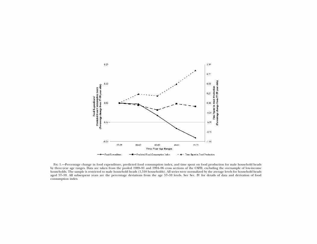
Fig 1.—Percentage change in food expenditure, predicted food consumption index, and time spent on food production for male household headsby three-year age ranges. Data are taken from the pooled 1989–91 and 1994–96 cross sections of the CSFII, excluding the oversample of low-incomehouseholds. The sample is restricted to male household heads (1,510 households). All series were normalized by the average levels for household headsaged 57–59. All subsequent years are the percentage deviations from the age 57–59 levels. See Sec. IV for details of data and derivation of foodconsumption index


TABLE 1Instrumental Variable Regression of Changes in Food Expenditure, ShoppingFrequency, and Time Spent on Food Production by Retirement Status, with

Demographic and Health Controls

Dependent VariableCoefficient on

Retirement Dummy

Expenditure:Log total food expenditure �.17

(.05)Log food expenditure at home �.15

(.05)Log food expenditure away from home �.31

(.11)Shopping frequency:

Dummy: shop for food at least once per week .17(.05)

Time spent on food production:Total time spent on food production (in minutes) 18.3

(6.9)Dummy: time spent on food production is positive .07

(.06)Log of time spent on food production, conditional on time

spent being positive.53

(.18)

Note.—Expenditure and shopping frequency data are taken from the pooled 1989–91 and 1994–96 cross sectionsof the CSFII. The sample is restricted to include only households with heads between the ages of 57 and 71 (2,052households). Log specifications are restricted to a subset of the sample that reports strictly a positive value for thedependent variable. Shopping frequency refers to the following question: “On average, how often does someone do amajor (grocery) shopping for this household?” The sample mean of the dummy variable for shopping at least onceper week is 0.66. Time use data are taken from the NHAPS. Food production (measured in minutes) is the sum oftime spent shopping for food and time spent preparing food. The sample restricts individuals in the NHAPS to bebetween the ages of 57 and 71 who had time spent on food production less than six hours (1,308 observations). Onlyeight individuals in the sample had daily food production in excess of six hours. The table reports the results from aninstrumental variable regression of the dependent variable on a dummy variable indicating whether the householdhead is retired and a vector of demographic, health, region, time, and education controls. One-year age dummies ofthe household head are used to instrument for retirement status. See the text for the full definition of demographic,health, region, time, and education controls included. Huber-White standard errors are in parentheses.

($377 vs. $423 per month; p-value of difference ! 0.01). These mag-nitudes are consistent with the evidence provided by Bernheim et al.(2001) and Haider and Stephens (2003), who use panel data.

The decline in consumption expenditures with age or at the time ofretirement is robust to the inclusion of a rich set of controls designedto capture changing demographics and health among older households.The first three rows of table 1 report the estimates of the followingregression:

ln (x ) p a � a retired � a Z � m , (1)it 0 1 it 2 it it

where is total food expenditure, expenditures on food at home, orxit

expenditures on food away from home, depending on the specification,for household i in year t; retiredit is a dummy variable equal to one ifthe household head i is retired in year t; and Zit is the vector of year,region, demographic, and health controls. Specifically, the Z vector in-cludes a series of controls for household composition including dum-


mies for time, the household’s family size and census region, and thehead’s education, race, sex, and responses to detailed health questions.9

Given that the timing of retirement can also be correlated with un-measured variables that affect the household’s expenditure decisions,we estimate (1) via an instrumental variable procedure. As is commonin the literature, we use age as our instrument for retirement. Agenaturally has strong predictive power for the household head’s retire-ment status. The adjusted of a regression of household retirement2Rstatus on age controls is 0.19 (with an associated F-statistic of 119.0).The top rows of table 1 report that when we add year, region, demo-graphic, and health controls, retired households spend 17 percent lesson total food (p-value ! 0.01), 15 percent less on food at home (p-valuep 0.01), and 31 percent less on food away from home (p-value p 0.01).10

While expenditure declines with retirement status, time spent on foodproduction dramatically increases with retirement status (we define foodproduction as shopping for food and preparing meals). Figure 1 showsthat male household heads aged 66–68 spend 21 percent more time onfood production than those aged 60–62. The pattern persists when wedirectly compare retired to nonretired households. For the NHAPS sub-sample of individuals aged 57–71, retired individuals spend 27 percentmore time on food production per day than their nonretired counter-parts (47 minutes vs. 37 minutes; p-value of difference ! .01). While wedo not report this, the data suggest that men experience a larger increasein food production time during retirement than women, although froma lower base.

To assess retirement’s impact on time use controlling for householddemographics, we estimate the following regression:

h p a � a retired � a Z � u , (2)it 0 1 it 2 it it

9 See the data appendix to Aguiar and Hurst (2004) for a full description of the healthquestion.

10 Haider and Stephens (2003) argue that self-reported retirement expectation is a betterinstrument for retirement than age. Using this instrument, they find that expendituredeclines by 8–10 percent at retirement. In the CSFII data, we observe only a cross sectionof households, and retirement expectations are not asked. Median regression (not re-ported) indicates that, in the CSFII data, the median decline in expenditure across re-tirement status is comparable to the mean decline.

As retirement has been defined according to the head’s status, it may be the case thata spouse continues to work. We find that roughly 30 percent of nonretired householdsin our age 57–71 sample have a spouse who works; that percentage falls by half for retiredhouseholds. As would be expected because of both permanent income and home pro-duction considerations, a working spouse raises expenditure by roughly 10 percent (p-value p 0.01) in nonretired households. The presence of a working spouse in retiredhouseholds raises expenditure by roughly 14 percent (p-value ! 0.01). The point estimatefrom estimating the interaction term suggests that a working spouse mitigates the fall inexpenditure due to retirement, but the scarcity of retired households with working spouseslimits the estimate’s precision.


where measures individual i’s propensity to shop for food or totalhit

daily time spent (in minutes) on food production. The CSFII asks house-holds whether they do their major shopping at least once a week. TheNHAPS, as mentioned above, records time spent shopping for food andtime spent preparing meals. For the NHAPS data, we also use as alter-native dependent variables a dummy variable indicating whether timespent on food production is positive and the log of time spent on foodproduction (if positive). The variable retired and Z are defined asabove.11 As before, we instrument for retirement status using agedummies.

The lower rows of table 1 show that retired households are 17 per-centage points (over a base probability of 66 percent) more likely todo their major food shopping on a weekly basis (p-value ! 0.01). Like-wise, retired households spend 18 more minutes per day on food pro-duction (p-value p 0.02) and spend 53 percent more time on foodproduction, conditional on food production being positive (p-value !

0.01). The breakdown between shopping and preparation (not re-ported) indicates that retirees spend 42 percent more time shoppingthan nonretirees and 54 percent more time preparing food, conditionalon demographics and positive time spent on the activity.12

Our primary analysis concerns food. However, the NHAPS also trackstime spent shopping for nongrocery household goods. During retire-ment, households increase their propensity to shop for other goods by50 percent and their total time spent shopping for other goods by 64percent. This suggests that expenditure may not be an accurate measureof actual consumption for nonfood goods.

It should be noted that 18 minutes a day is a sizable increase in timespent on food production. The 18 minutes per day translates into anadditional nine hours per month of food production. If householdsvalue their time during retirement at half the sample’s average prere-tirement wage of $18, this would translate into an additional $81 permonth of food production. During retirement, total monthly expen-diture on food, conditional on demographics, declines by about $70per month. That is, if one values the time of retired households at halftheir preretirement wage, the increase in time spent on food productionfor retired households is roughly the same as their decline in foodexpenditure.

11 Given that the demographic variables recorded in the NHAPS data are much morelimited, the Z vector for time spent on food production includes only year, region, sex,household size, education, and race controls. The NHAPS data set does not include anyhealth measures.

12 The fact that time spent on home production and shopping increases with retirementstatus is consistent with the majority of work that examines time use. See, e.g., Juster andStafford (1985), Blaylock (1989), Cronovich, Daneshvary, and Schwer (1997), Hurd andRohwedder (2003), and Aguiar and Hurst (2005).


IV. Nutrition, Consumption Categories, and Luxury Goods inRetirement

The CSFII data provide tremendously detailed accounts of an individ-ual’s dietary habits. To assess whether an individual’s food consumptionchanges in retirement, we explore the data in four ways. First, we ex-amine the nutritional composition of the individual’s diet. Second, weexamine individual categories of food consumption. In both cases, weidentify nutritional measures and consumption categories that exhibitstrong income elasticities. Third, we explore consumption goods thathave an observable quality component. Finally, we form a consumptionindex that aggregates numerous individual consumption categories andtest whether this index varies with retirement status.

The CSFII reports summary statistics for each individual’s daily diet.We start our analysis by focusing on eight nutritional measures: totalcalories, vitamin A, vitamin C, vitamin E, calcium, saturated fat, cho-lesterol, and protein. Our methodology has two components. First, weestablish that these nutritional measures vary with lifetime resources.Second, we show whether the consumption of these nutritional mea-sures changes with retirement status.

Panel A of table 2 reports the income elasticity of these nutritionalmeasures for a sample of household heads between the ages of 45 and55 who are working full-time.13 To obtain this elasticity, we estimate aninstrumental variable regression of the log of the nutrition measure onthe log of income as well as add controls for race, sex, family compo-sition, height, and health. We instrument current household incomewith occupation, education, education and occupation interactions, andsex and race interactions. Aside from the log calories regression, allother regressions in panel A include log calories as an additional control.In panel B, we regress this same dependent variable on a dummy variableequal to one if the household head is retired (instrumented with agedummies). This sample is the same used to compute the estimates intable 1 (household heads aged 57–71). As with the results in table 1,this regression also includes race, sex, year, region, household com-position, and health controls.

As perhaps should be expected, log calories vary slightly with per-manent income within a cross section of middle-aged, working house-holds, with an estimated elasticity of 0.06 (p-value p 0.02). However,other dietary components respond strongly to variation in income. Spe-

13 We computed the income elasticities reported in tables 2 and 3 for households workingfull-time on two alternative samples: (1) household heads aged 25–55 and (2) householdheads aged 57–71. The results for the former sample are discussed in Aguiar and Hurst(2004). The estimated income elasticities were nearly identical across the three differentsamples we analyzed.


TABLE 2Income Elasticity of Nutritional Measures among Working Households and

Change in Nutritional Measures across Retirement

DependentVariable

A. Estimated IncomeElasticity:

Sample: Heads Aged 45–55Working Full-Time

B. Estimated RetirementEffect:

Sample: All HouseholdHeads Aged 57–71

Coefficienton Log

PermanentIncome

(1)

Mean ofDependent

Variable(2)

Instrumental VariableCoefficient on

Retirement Status Dummy(3)

Log calories .06(.03)

7.59 �.02(.03)

Log vitamin A .54(.08)

8.48 .36(.09)

Log vitamin C .41(.08)

4.22 .33(.09)

Log vitamin E .24(.04)

2.03 .11(.04)

Log calcium .10(.04)

6.51 .13(.04)

Log cholesterol �.22(.05)

5.55 �.09(.05)

Log saturated fat �.10(.03)

3.18 �.07(.03)

Log protein .004(.02)

4.18 �.03(.02)

Note.—Data come from the pooled CSFII_89 and CSFII_94 data sets. Sample sizes are 1,101 household heads forpanel A and 2,052 household heads for panel B. All nutritional measures aside from calories, protein, and saturatedfat are measured in milligrams. Saturated fat and protein are measured in grams. Col. 1 reports the coefficient on logincome from an instrumental variable regression of the nutritional measure on log income and race, sex, height, health,year, and region controls, where indicators of permanent income are used as instruments for log income. The instrumentsinclude occupation, education, education and occupation interactions, and sex and race interactions. Huber-Whitestandard errors are in parentheses. See the text for a discussion. Panel B reports the coefficient on a dummy variableindicating whether the household head was retired from an instrumental variable regression of the nutritional variableon the retirement dummy and demographic and health controls. Retirement status was instrumented with age dummies.All regressions in both panels, except when log calories is the dependent variable, include log calories as an additionalcontrol.

cifically, the income elasticities of vitamin A and vitamin C are over 0.40(p-values ! 0.01), and the income elasticities of vitamin E and calciumare 0.24 and 0.10, respectively (p-values ! 0.01). Likewise, cholesteroland saturated fat are inferior goods (income elasticities equal to �0.22and �0.10, respectively; p-values ! 0.01). The results are robust to theinclusion of controls for whether the household head is taking specificvitamin supplements. Furthermore, nonlinear estimation (not reported)confirms that vitamins (either A, C, or E) are a strictly increasing func-tion of income over all observed income ranges. Likewise, cholesterolis a strictly declining function of income over all observed incomeranges. The results are consistent with individuals consuming inexpen-sive calories by switching their diet toward fat and cholesterol and awayfrom vitamins and calcium. The suggestion that “fat” is cheap and


“healthy diets” are expensive is consistent with a large literature onnutrition and income (see, e.g., Subramanian and Deaton 1996; Bhat-tacharya, Currie, and Haider 2003).14

The results from panel A of table 2 suggest that if an individual entersretirement with too few resources, we may observe the composition ofhis or her diet shifting away from vitamin-rich foods toward fat andcholesterol. As seen in panel B, there is no evidence that the nutritionalquality of a household’s diet deteriorates during retirement. In fact,retired households consume higher-quality diets (as measured by morevitamins and less cholesterol) than their working counterparts. If thedecline in expenditure represented a fall in actual consumption, wewould expect to observe either a decline in total calories or a deterio-ration of the quality of calories. The data support neither of thosepredictions.

Moving beyond nutritional aggregates, we also observe detailed foodintake for each individual. The CSFII data track the quantities consumed(in grams) in a given day using thousands of eight-digit food codes. Thestructure of these food codes is similar to that of Standard IndustrialClassification occupation and industry codes. As a result, we can aggre-gate these food codes up to broader classifications. For much of ouranalysis, we use three-digit food codes (e.g., natural cheeses, cottagecheeses, processed cheeses, etc.). The reason we do not always exploitthe eight-digit food code categories is that often there are only a handfulof households that consume any given specific type of food category ona given day. There are some instances below, however, in which we douse the eight-digit food codes. We have explored hundreds of the in-dividual three-digit and eight-digit consumption categories. Table 3 re-ports the results from only a few of these categories. The categories wechose were ones that had strong income elasticities among workinghouseholds or ones that were suggested to us by other researchers. Whileonly a handful of the categories are presented, it should be stressedthat we found no evidence that upon retirement individuals experienceda systematic decline in consumption among all the goods we explored.

Table 3 has essentially the same structure as table 2. Panel A measuresthe income semielasticity of the incidence of consuming a positiveamount of a given food category. The sample and controls are identical

14 One potential concern with the regression is that income may be correlated withnutritional literacy or other preferences for a healthy diet. To address this, we use CSFIImeasures of nutritional preference and nutritional literacy. Households are specificallyasked about their preference regarding a healthy diet and whether they are informedabout the dangers of unhealthy diets. We included a number of these controls in thespecifications reported in tables 2 and 3 and found little impact on the reported coeffi-cients. More to the point, the exercise is designed to highlight aspects of diet that distin-guish rich from poor households in the cross section and then to test whether retirees’lower expenditure is manifested as a “low-income” diet.


TABLE 3Income Semielasticity of Food Categories among Working Households and

Change in Propensity to Consume Food Categories in Retirement

DependentVariable

A. Estimated IncomeSemielasticity:

Sample: Heads WorkingFull-Time Aged 45–55

B. Estimated RetirementEffect:

Sample: All HouseholdHeads Aged 57–71

Coefficienton Log

PermanentIncome

(1)

Mean ofDependent

Variable(2)

Instrumental VariableCoefficient on

Retirement Status Dummy(3)

Dummy: eat fruit .23(.05)

.65 .14(.04)

Dummy: eatshellfish

.06(.02)

.06 �.02(.02)

Dummy: drink wine .15(.03)

.09 �.03(.03)

Dummy: eat yogurt .17(.03)

.10 .01(.03)

Dummy: eat oat/rye/multigrainbread

.12(.03)

.13 .06(.04)

Dummy: eat hotdogs/lunch meat

�.16(.05)

.50 �.06(.05)

Dummy: eat groundbeef

�.11(.04)

.20 �.01(.04)

Note.—Data come from the pooled CSFII_89 and CSFII_94 data sets. Sample sizes are 1,101 household heads forpanel A and 2,052 household heads for panel B. The dependent variable is a dummy variable taking the value one ifthe respondent consumed the listed item, and zero otherwise. Col. 1 reports the coefficient on log income from aninstrumental variable regression of the dummy variable on log income and race, sex, height, health, year, and regioncontrols, where indicators of permanent income are used as instruments for log income. The instruments includeoccupation, education, education and occupation interactions, and sex and race interactions. Huber-White standarderrors are in parentheses. See the text for a discussion. Panel B reports the coefficient on a dummy variable indicatingwhether the household head was retired from an instrumental variable regression of the consumption dummy on theretirement dummy and demographic and health controls. Retirement status was instrumented with age dummies.

to those of table 2. The dependent variable is a dummy variable equalto one if the individual consumed any of the consumption category. Wereport seven food categories: fresh fruit, shellfish, wine, yogurt, oat/rye/multigrain bread, hot dogs/lunch meat, and ground beef. As seenfrom panel A of table 3, the first five categories all exhibit strong positiveincome semielasticities. For example, a doubling of income increasesthe probability that a household eats fresh fruit by 23 percentage points(p-value ! 0.01), with 65 percent of the sample consuming fresh fruit.Conversely, hot dogs/lunch meat and ground beef have negative semi-elasticities. As seen in panel B of table 3, there is no evidence thatindividuals switch away from goods with high income elasticities at thetime of retirement. For these categories, the consumption patterns ofretirees look very similar to those of their nonretired counterparts. Theonly statistically significant change suggests that retirees eat better.

The analysis so far may be subject to the criticism that we are missing


quality differences within categories. For example, it may be that house-hold consumption of ground beef does not change at the time of re-tirement. Instead, retired households consume cheaper, low-qualityground beef, whereas preretired households consume more expensive,higher-quality ground beef. In table 4, we examine goods with an ob-servable measure of quality.

First, the CSFII data set tracks where each meal is consumed. Spe-cifically, if a meal is consumed away from home, we know whether it isat a fast-food restaurant, a cafeteria, a bar, or a restaurant with tableservice. A restaurant with table service provides more ambiance andhigher-quality food than a fast-food establishment. As seen in table 4,the “luxury good” quality of restaurants is clear in the data: within across section of household heads aged 45–55 who are working full-time,a doubling of income increases the incidence of eating at a restaurantwith table service by 16 percent (p-value ! 0.01). The income elasticityfor fast food is lower, although still positive. The positive income elas-ticity on fast food and cafeteria food may reflect in part how the natureof the work environment and the opportunity cost of time vary withincome. Restaurant meals may also capture work-related activity as wellas pure consumption. Nevertheless, it seems safe to conclude that thehigher income elasticity for restaurants with table service versus fast-food restaurants to a large extent reflects quality differences.

However, there is no evidence that individuals decrease their pro-pensity to eat at restaurants with table service upon retirement. Table4 reports that retired households are 18 percentage points less likely toeat out, consistent with the 31 percent difference in expenditure onfood away from home. However, the decline in eating away from homeoccurs because individuals cease to eat at fast-food restaurants and caf-eterias. In fact, the propensity to eat at a restaurant with table serviceis 29 percent for both individuals aged 60–62 (before peak retirementyears) and individuals aged 66–68 (after peak retirement years).15

One question that arises is how much of the observed drop in ex-penditure on meals away from home is accounted for by the decline infast-food and cafeteria meals. The lack of direct measures of expenditureacross the different types of establishments necessitates an indirect cal-culation. All else equal, a retired household spends 31 percent less on

15 As mentioned in n. 10, there are some elderly households in which the spouse works(including those in which the head is retired). We find that having a working spouse raisesexpenditure by roughly 11 percent among (all) elderly households, all else equal. However,the evidence suggests that the nonworking spouse mitigates the effect of this decline inexpenditure on consumption. That is, in a regression of our consumption measures ona ‘‘working spouse” dummy variable plus our usual controls, the coefficient on the workingspouse dummy variable is typically close to zero. The prominent exception is that house-holds in which the wife works are significantly more likely to eat out at restaurants withtable service.

TABLE 4Income Semielasticity of Restaurants with Table Service and High-Quality Food among Working Households and Change in

Propensity to Consume in Retirement

Dependent Variable

A. Estimated Income Semielasticity:Sample: Heads Aged 45–55 Working

Full-Time

B. Estimated Retirement Effect:Sample: All Household Heads Aged

57–71

Coefficienton Log

PermanentIncome

(1)

Mean ofDependent

Variable(2)

Instrumental Variable Coefficient onRetirement Status Dummy

(3)

Propensity to eat away from home:Dummy: individual eats away from home (all

establishments).16

(.04).72 �.18

(.05)Dummy: individual eats at a cafeteria .12

(.03).13 �.07

(.03)Dummy: individual eats at a fast-food

establishment.10

(.05).42 �.16

(.04)Dummy: individual eats at a restaurant with

table service.16

(.05).41 �.03

(.05)Propensity to switch away from high quality:

Dummy: individual eats “lean” ground beef* .44(.12)

.53 .13(.13)

Note.—Data come from the pooled CSFII_89 and CSFII_94 data sets. Sample sizes are 1,101 household heads for panel A and 2,052 household heads for panel B. The dependent variable is adummy variable taking the value one if the respondent consumed the listed item, and zero otherwise. Eating away from home is defined as eating any meal at a cafeteria, bar, fast-food establishment,or restaurant with table service. The eight-digit food codes categorize whether the beef consumed by individuals was lean or not. Col. 1 reports the coefficient on log income from an instrumentalvariable regression of the dummy variable on log income and race, sex, height, health, year, and region controls; indicators of permanent income are used as instruments for log income. Theinstruments include occupation, education, education and occupation interactions, and sex and race interactions. Huber-White standard errors are in parentheses. See the text for a discussion.Panel B reports the coefficient on a dummy variable indicating whether the household head was retired from an instrumental variable regression of the consumption dummy on the retirementdummy and demographic and health controls. Retirement status was instrumented with age dummies.

* The sample was additionally restricted to include only those household heads who reported eating ground beef (159 for panel A and 270 for panel B).


food away from home than a nonretired household (table 1). For non-retired household heads aged 57–71, the average monthly expenditureon food away from home is $85, implying a difference in levels of roughly$26 per month. Table 4 indicates that retired households are 0.20 per-centage points less likely to frequent fast-food restaurants or cafeterias,or roughly six fewer trips per month. In order for fast-food and cafeteriameals to account for the entire decline, households must spend, onaverage, $4.33 per trip. The fact that this number is not particularlylarge is consistent with the hypothesis that much of the decline in ex-penditure on food away from home can be accounted for by less fre-quent visits to fast-food and cafeteria establishments.

Another quality characteristic for which we have data is the leannessof meat. Specifically, the eight-digit food codes distinguish betweenwhether the household consumed regular or lean ground beef. Whileground beef is an inferior good, table 3 documented that the propensityto eat ground beef does not increase with retirement status. Amongworking households, conditional on eating ground beef, the choice oflean ground beef is positively related to income, with a semielasticity of0.44. However, retirees are just as likely as their nonretired counterpartsto consume high-quality ground beef. The results are also shown intable 4.

Additionally, we can directly test whether individuals switch towardlower-quality goods, within a given food category, upon retirement. Formost food items, information on the brand of that good is unavailable.However, we do have brand information for cereal. We find that amonghousehold heads aged 57–71 who eat cereal, 13 percent of retirees eat“store brand” cereal, roughly identical to the 14 percent rate amongnonretirees (p-value of difference p 0.67).

The categories highlighted in the analysis thus far represent only asmall fraction of the CSFII data available. The difficulty with exploitingthe full range of data is how to aggregate the various components. Ourapproach is to derive the weights for the individual food categorieswithin our consumption index by projecting the permanent income ofprime-aged working households on the quantities consumed of varioustypes of foods. As we have shown above, there is a relationship betweena household’s permanent income and the composition of its diet. Toexplore this relationship formally, we estimate our consumption indexas follows:

perm,i i i i i i…ln (y ) p b � a c � � a c � b ln (x ) � b v � b age0 1 1,t J J,t X t v t age t

i 2 i� b (age ) � e , (3)2age t t

where is an estimate of the household’s permanent income;permy c ,1

represent the quantity consumed of food ; v is a vector… , c j p 1, … , JJ


of taste controls; age is the age of the individual; and x is the totalmonthly expenditure for the individual’s household. As shown in Aguiarand Hurst (2004), the inclusion of expenditures along with quantitiescontrols for differences in prices paid across households.16

We estimate (3) on a sample of household heads from our CSFII datawho are between the ages of 25 and 55 and who report working full-time (2,966 individuals). The permanent income for each employedhousehold head is estimated as above using race, sex, industry, andoccupation controls.17 For our consumption measures, we selected 79three-digit food categories (listed in Appendix table A1) plus our eightnutritional measures displayed in table 2. The vector of taste controls(v) includes the household head’s race, sex, family composition, mul-tiple health status controls, and region of residence.

To explore how well food consumption predicts income, we split thesample into two. We estimated (3) for full-time employed individualsaged 25–55 in the odd years of our survey. The of this regression was2R0.53. Food consumption items on their own explain 21 percent of thevariation in permanent income, whereas the incremental of the ad-2Rdition of the food variables to the expenditure, age, and taste controlswas 12 percent. Using the regression coefficients, we predicted per-manent income out of sample for full-time employed individuals aged25–55 in the even years of the sample. The from the out-of-sample2Rregression of actual income on predicted income was 0.42 (omittingdemographics and expenditure and using food alone produced an out-of-sample of 0.09). This out-of-sample forecasting power indicates2Rthat diet is fairly informative regarding a household’s permanentincome.

There are two things to note with respect to the estimation of (3).First, we do not have the actual permanent income for retired house-holds. However, the goal of this paper is to ask whether retired house-holds act as though their lifetime resources have unexpectedly declinedonce they entered retirement. Using (3), we can predict a household’simplied permanent income on the basis of what its members eat. Spe-cifically, we obtain the parameters of the aggregation function from theestimates of (3) and form for each in-ˆˆ …ˆ ˆln C { a c � � a c � b ln X1 1 1 1 X

dividual (including retired households), where again expenditure isincluded to control for price heterogeneity. Given the specification, theunits of our consumption index are in log permanent income dollars.

16 Also, as shown in Aguiar and Hurst (2004), aside from simply being interpreted asan estimate of a consumption index, this expression can be used to derive an approxi-mation to the Lagrange multiplier on lifetime resources in a canonical life cycle modelaugmented to include home production.

17 We bootstrap standard errors in (3) to adjust for the fact that permanent income ispredicted for each household.


TABLE 5Instrumental Variable Regression of Changes in

Consumption Index and Predicted Expenditure byRetirement Status, with Demographic and

Health Controls

Dependent Variable Coefficient

1. Log of food consumptionindex

�.006(.02)

2. Log of predicted foodexpenditure

�.004(.014)

Note.—The dependent variable for regression 1 is the predicted logfood consumption index using reported food consumption measures andtotal monthly food expenditures (from eq. [3]). The reported coefficientfor row 1 is g1 from (4). The dependent variable for regression 2 is predictedexpenditure using reported food consumption measures. Data for rows 1and 2 are taken from the pooled 1989–91 and 1994–96 cross sections ofthe CSFII. The sample is restricted to include only households with headsbetween the ages of 57 and 71 (2,052 households). See the text for ad-ditional details and the list of additional regressors. Bootstrap standarderrors from 500 repetitions are reported in parentheses.

A 1 percent decline in our consumption index implies that householdsare consuming as though their permanent income had fallen by 1 per-cent. Figure 1 plots for male household heads in the CSFII dataˆln Cbetween the ages of 57 and 71, by three-year age ranges. While expen-diture falls dramatically for households in the peak retirement age, theconsumption index remains essentially constant. Indeed, the pure“quantity” component of the index, obtained by subtracting fromb ln XX

, increases slightly in retirement. This is the optimal response to theˆln Clower cost of consumption in retirement, with the small size of theincrease being consistent with a low intertemporal elasticity of substi-tution for food.

Using the same procedure we followed with expenditure, we regressthe consumption index on retirement status and taste controls. Formally,we estimate

ˆln C p g � g retired � g Z � n , (4)0 1 it 2 it it

where retired and Z are defined in (1) and (2). As before, we instrumentretirement status with age controls. The results are reported in the firstrow of table 5. We find no evidence that our consumption index variesacross retirement status. The coefficient on g1 is �0.006. We have per-formed a number of robustness checks and found that the impact ofretirement remains negligible across numerous alternative specifications(see Aguiar and Hurst [2004, app. 2] for details).

In the preceding analysis, we formed our consumption index by pro-jecting permanent income on consumption patterns. An alternativemethodology projects expenditure on consumption patterns. The es-timated index weights under this approach will be the implied prices


for the benchmark group of working households. With these prices, wethen can compare the implied cost (at “benchmark prices”) of theconsumption of retirees with that of nonretirees.

To perform this analysis, we reestimate (3), but with log expenditureas our dependent variable rather than income (removing expenditureas a control). Note that the fit of this regression is hampered by thefact that our quantities represent food intake by an individual over afew days, whereas expenditure represents household purchases over theentire month. Nevertheless, we find that food diaries have substantialpredictive power. The adjusted of the first stage is 0.28, and the2Rincremental adjusted associated with the inclusion of food controls2Ris 0.05. Moreover, the correlation between a household’s predicted ex-penditure and that household’s predicted permanent income is 0.6.

We then predict the implied expenditure for each retired householdusing its consumption bundle and the estimated coefficients: ˆln x pi

. Then we regress this measure using the samei i ˆ…ˆ ˆa c � � a c � b v1 1 J J v

controls as (4). The coefficient on retirement status is shown in row 2of table 5. Like our predicted consumption index, predicted expendi-ture does not vary with retirement status (coefficient p �0.005; p-valuep 0.67). Even though actual expenditure is falling sharply with retire-ment status, predicted expenditure based on the household’s con-sumption bundle remains constant. This further suggests that pricespaid by retired households are falling sharply during retirement.18

One interesting result documented by Bernheim et al. (2001) con-cerns the heterogeneity of declines in expenditure at retirement acrossincome and wealth groups. In particular, they find that the lowest quar-tile of the wealth distribution experiences a disproportionate declinein expenditures. Our analysis so far has focused on the average behaviorof households. Unfortunately, our data set does not contain detailedwealth or pension data. With respect to wealth, individuals in the CSFIIare asked the amount of liquid wealth they have only if it is below $5,000.Additionally, we know whether the household owns its own home. Withthese data in hand, we identify a subset of “low-wealth” householdsdefined as those with less than $1,000 in liquid assets and that do notown their home. This subset contains 369 individuals, or roughly 10percent of our sample.19

Compared with the full sample of households and consistent with

18 The fact that households pay lower prices for a given consumption good (as measuredby universal product code) has been documented by Aguiar and Hurst (2005). They findthat, on average, households over the age of 65 pay approximately 5 percent lower pricesfor a given universal product coded good than middle-aged households.

19 For this analysis, we included the oversample of low-income households to increaseour sample size. The low-income households were included only if they met our definitionof low wealth.


Bernheim et al. (2001), low-wealth individuals experience a larger de-cline in expenditures at retirement (25 percent [p-value p 0.04] vs. 17percent [p-value p 0.01]). However, given the small sample, power isan issue. In particular, we cannot precisely estimate the effect of retire-ment on consumption of low-wealth households for many of our con-sumption measures. One pattern we can identify concerns restaurantmeals: compared with nonretired low-wealth households, low-wealth re-tirees are less likely to dine at restaurants with table service (�12-per-centage-point decline; p-value p 0.10). We also find that low-wealthretirees consume roughly the same amount of fruit as low-wealth non-retirees (4 percent increase; p-value p 0.71) and are much less likelyto consume calories (19 percent decline; p-value p 0.04). The com-parable numbers for the full sample were, respectively, �3 percentagepoints, 23 percent, and 6 percent. Overall, we conclude that averagehouseholds are modeled well by the PIH in the sense that they smoothconsumption across predictable income shocks such as retirement. How-ever, there may be a segment of the population with very low wealththat experiences a measured consumption decline upon retirement.

One final piece of corroborating evidence comes from a questionposed in the 1968 PSID. Specifically, households were asked, “Are thereany special ways you try to keep the food bill down?” If the respondentsanswered yes, the PSID asked them to list which (perhaps more thanone) methods were used. In the sample of 816 household heads aged57–71, retirees were slightly more likely than nonretirees to answer yesto this question (57 and 51 percent, respectively). However, conditionalon their answering yes and with controls added for sex, education, andmarital status, retirees were 9.5 percentage points less likely than non-retirees to respond that they reduced their food expenditures by “eatingcheaper or lower-quality foods” (p-value p 0.07). Moreover, the re-sponse “eating less” was as common among nonretirees as among re-tirees. However, retirees were seven percentage points more likely tolist shopping for bargains, making own meals, or growing own food asmethods to reduce food costs (p-value p 0.38).20

In this section, we have marshaled evidence indicating that house-holds do not suffer declines in consumption (as opposed to expendi-ture) at retirement. A typical concern with finding that a variable hasno effect is the power of the test. That is, are we confident that ourprocedure would detect a significant effect if one indeed existed? Thefact that our forecasts based on consumption predict both permanentincome and expenditure out of sample is one argument to mitigate this

20 Of nonretirees who reported taking action to reduce their food bill, 15 percent listed“eating cheaper or lower-quality foods,” and 42 percent reported “shopping for bargains,”“making own meals,” or “growing own food.”


concern. Second, as we discuss in the next section, our consumption-based measure of income responds to unemployment status.

V. Consumption Changes during Unemployment

In this section, we use the data and methodology developed in theprevious section to analyze the changes in consumption when workersbecome unemployed. To the extent that unemployment represents anunanticipated shock to lifetime resources, the PIH does not predict thatconsumption will remain constant across unemployment status. How-ever, theory does suggest that unemployed agents should spend moretime in home production to reduce the price paid for a unit ofconsumption.

For our analysis, we use the sample of household heads between theages of 25 and 55 who are either full-time employed or unemployed.We do not exclude the oversample of the poor from the 1989–91 CSFIIsurvey, which provides more unemployed and comparable employedindividuals. We also reestimate each specification restricting the sampleto heads with 12 years or less of schooling. This “low-education” sub-sample contains a set of employed individuals who are perhaps morecomparable to the unemployed, partially mitigating the concern thatwe are comparing inherently different employed and unemployedhouseholds in the cross section. Our full sample consists of 3,874 house-hold heads, 7 percent of whom are unemployed. Our low-educationsample consists of 1,927 household heads, with 10 percent being un-employed. Likewise, we create similar samples within the NHAPS dataset, with 3,364 (4.6 percent unemployed) and 1,258 (7.0 percent un-employed) individuals, respectively.

As with retirement, we first document that unemployed householdsspend less on food than their employed counterparts. To control forother observables, we estimate

ln (x ) p b � b unemployed � b Z � v , (5)it 0 1 it 2 it it

where is total food expenditure, expenditures on food at home, orxit

expenditures on food away from home, depending on the specification,for household i in year t; unemployedit is a dummy variable equal toone if household head i is unemployed in year t. As before, the Z vectorincludes the same series of health and demographic controls includedwhen estimating (1)

The results of estimating (5) are reported in columns 1 (full sample)and 2 (low-education sample) of table 6. For the full sample, total ex-penditure on food falls by roughly 19 percent in unemployment (p-value ! 0.01), with food at home falling by 9 percent (p-value p 0.02)and food away from home falling by 42 percent (p-value ! 0.01). For


TABLE 6Regression of Changes in Food Expenditure, Shopping Frequency, and Time

Spent on Food Production by Unemployment Status, with Demographic andHealth Controls

Dependent Variable

Full Sample:Coefficient on

Unemployment Dummy(1)

Low-Education Sample:Coefficient on

Unemployment Dummy(2)

Expenditure:Log total food expenditure �.19

(.03)�.21(.04)

Log food expenditure athome

�.09(.03)

�.15(.04)

Log food expenditure awayfrom home

�.42(.07)

�.38(.09)

Time spent on food produc-tion:

Total time spent on foodproduction (in minutes)

11.6(4.1)

11.6(5.4)

Dummy variable: spend posi-tive time on foodproduction

.08(.04)

.07(.05)

Log of time spent on foodproduction, conditional ontime spent being positive

.28(.09)

.26(.12)

Consumption:Log of food consumption

index�.05(.01)

�.04(.02)

Note.—Expenditure and consumption data are taken from the CSFII data sets. For both cols. 1 and 2, the samplewas restricted to include households with heads between the ages of 25 and 55 who either were working full-time orwere unemployed. The additional sample of low-income households from the 1989–91 survey is also included. Thesample size for col. 1 is 3,874 household heads. In col. 2, we imposed the additional restriction that the householdhead had accumulated 12 years or less of schooling. The sample size for col. 2 is 1,927 household heads. Log specificationsinclude only those households with a strictly positive dependent variable. See the text for additional details. The dataon time use come from the NHAPS data (3,364 observations for the full sample and 1,258 for the low-education sample).This sample was restricted to include individuals between the ages of 25 and 55 who either were working full-time orwere unemployed. Food production refers to shopping for food or preparing meals. Coefficients come from an ordinaryleast squares regression of the dependent variable on an unemployment dummy and a series of demographic, year,region, health, and education controls. See the text for a full description of the variables included. See Sec. IV fordetails of data and derivation for food consumption index. Huber-White standard errors are in parentheses. The standarderrors for the consumption index are bootstrapped (500 repetitions).

the low-education sample, the comparable numbers are �21 percent,�15 percent, and �38 percent (p-values for all ! 0.01). These numbersare comparable in magnitude to those reported by other researchers.21

The fact that our cross-sectional declines in expenditure are of a mag-nitude similar to those found using panel data is reassuring regardingthe ability of our demographic variables to control for inherent differ-ences between employed and unemployed households.

21 Using the PSID, Stephens (2001) finds that household food expenditure declines byroughly 10 percent following involuntary job loss of the household head. Using the BritishFamily Expenditure survey, Banks et al. (1998) find that unemployed households expe-rience a 7.6 percent decline in food at home and domestic energy and a 52 percentdecline in work-related expenses that include restaurant meals, transport, and adultclothing.


As predicted by theory, unemployed households spend more timeshopping and preparing food. Columns 1 and 2 of table 6 report re-gressions of time use on unemployment status, controlling for demo-graphics. Unemployed individuals spend, on average, 12 minutes morethan employed individuals in food production or 28 percent more timeconditional on reporting a positive amount of time (p-values ! 0.01).The numbers are similar when we restrict analysis to the low-educationsample.

The last row of table 6 indicates that unemployed households ex-perience a significant change in actual consumption. As discussed inSection IV, we use observed food consumption and food expendituremeasures for each household to fit a consumption index for each in-dividual in the unemployment sample. With all employed householdsused as a comparison group, column 1 of table 6 reports that unem-ployed household heads experience a 5 percent drop in consumption(p-value ! 0.01). For the comparison group of low-educated employedhouseholds, column 2 of table 6 reports that unemployed householdheads experience a 4 percent drop in consumption (p-value ! 0.01).We have performed a number of robustness checks and found that overthe alternative specifications, the estimated drop in implied lifetimeresources for the unemployed ranged from 4 percent to 8 percent. Ineach case, we were able to reject a zero change in our consumptionindex or predicted expenditure at standard confidence levels (seeAguiar and Hurst [2004] for details).

Finally, we look more closely at the effect of unemployment on foodaway from home. As noted above, expenditure in this category dropsroughly 40 percent, 10 points more than the 30 percent decline observedin retirement. Recall that a retiree’s decline in the propensity to eataway from home was largely confined to the reduced frequency of fast-food and cafeteria meals. Table 7 breaks down the propensity to eatfood away from home by type of establishment for the unemployed,controlling for the full set of demographics and health variables. PanelA of table 7 focuses the analysis on the full unemployment sample, andpanel B focuses the analysis on the low-education unemployment sam-ple. The first row reports that the probability of eating out declines byroughly 25 percentage points in unemployment, compared to a samplemean of 70 percent. As with retirees, the probability of eating fast-foodor cafeteria meals shows dramatic declines in unemployment, with fastfood declining 20 percentage points (vs. a sample mean of 43 percent)and cafeteria meals declining eight points (vs. a sample mean of 8percent). Both declines are statistically significant at the 1 percent level.However, unemployed household heads also experience a large declinein visits to restaurants with table service. For the low-education sample,the incidence of dining out at such establishments declines 15 per-


TABLE 7Propensity to Eat Away from Home among Working-Age Households, by

Unemployment Status

Dependent Variable

A. Full Sample B. Low-Education Sample

Coefficient onUnemployment

Dummy(1)

Mean ofDependent

Variable(2)

Coefficient onUnemployment

Dummy(3)

Mean ofDependent

Variable(4)

Dummy: household eatsaway from home (allestablishments)

�.25(.03)

.70 �.27(.04)

.65

Dummy: household eatsat restaurant with ta-ble service

�.18(.02)

.34 �.15(.03)

.28

Dummy: household eatsat a cafeteria

�.10(.01)

.12 �.08(.01)

.09

Dummy: household eatsat a fast-foodestablishment

�.17(.03)

.45 �.20(.03)

.43

Note.—Data are taken from the pooled 1989–91 and 1994–96 cross sections of the CSFII, collected by the Departmentof Agriculture. The sample is restricted to include households with heads between the ages of 25 and 55 who eitherwere working full-time or were unemployed. The additional sample of poorer households from the 1989–91 survey isincluded. Data refer to the consumption patterns of only the household head. The sample size for panel A is 3,874household heads. In panel B, we imposed the additional restriction that the household head had accumulated 12 yearsor less of schooling. The sample size for panel B is 1,927 household heads. Eating away from home is defined as eatingany meal at a cafeteria, bar, fast-food establishment, or restaurant with table service. Cols. 1 and 3 report the resultsfrom an ordinary least squares regression of a dummy variable indicating whether the household ate a meal away fromhome on a dummy variable indicating whether the household head was unemployed and a vector of demographic,health, region, time, and education controls. See the text for the full definition of demographic, health, region, time,and education controls included. Huber-White standard errors are in parentheses.

centage points (p-value ! 0.01) in unemployment, with a sample meanfrequency of 28 percent. In contrast to the retirees, the unemployedtherefore experience a significant loss in terms of the quality of theirconsumption of meals away from home.

Consistent with the decline in the consumption index and the pro-pensity to eat at restaurants with table service, unemployed householdsexperience declines in quality of food consumption along other di-mensions. Specifically, relative to their employed counterparts, unem-ployed households consumed 16 percent less vitamin C, 12 percent lessvitamin A, and 14 percent less vitamin E. Additionally, unemployedhouseholds were five percentage points more likely to consume hotdogs, three percentage points less likely to consume shellfish, and ninepercentage points less likely to consume fresh fruit.

The data on the quality and quantity of food consumed indicate thatunemployed households experience a measurable drop in utility. Thedecline in lifetime resources implied by the pattern of consumption andexpenditure is roughly 5 percent. This number is similar to the estimatesof the shock to permanent income due to job loss. For example, Stevens(1997) estimates that job displacement reduces earnings (relative tobefore unemployment) by roughly 9 percent six or more years after the


onset of unemployment. The change in consumption during unem-ployment provides an interesting counterpoint to the notable absenceof such a decline during retirement. This further suggests that if therewere a meaningful decline in consumption associated with retirement,our tests have enough power to detect it.

VI. Discussion and Conclusion

The data on food consumption analyzed in this paper indicate thatconsumption is much more stable across individuals with similar per-manent income but different current income than expenditures are.The evidence suggests that agents are able to smooth consumption bysubstituting time for expenditures. One concern with our study is thatwe analyze a cross section of individuals when the PIH concerns anindividual over time. We have a fairly rich set of demographic and healthvariables that help control for individual heterogeneity. More important,we find fluctuations across individuals in expenditures that are not pres-ent in consumption. In particular, we quantitatively match the behaviorof expenditures during retirement and unemployment that have beendocumented by other researchers with panel data sets, while at the sametime documenting that consumption behaves much differently thanexpenditures.

The key issue is whether our measures of food intake capture theutility of food consumption. Throughout the paper, we measure foodquantity and quality along a number of dimensions. All the measurestell a consistent story. The individual income elasticities, the out-of-sample checks, and the fact that the unemployed show a decline inconsumption confirm that our measures are able to detect a decline inpermanent income when present. Our analysis indicates that consump-tion is stable, both absolutely and relative to expenditures, during an-ticipated shocks to income such as retirement. If there is a margin ofsubstitution through which utility from the consumption of food de-clines during retirement, it is not apparent from extremely detailedfood diaries.

While food consumption represents only a portion of the household’stotal consumption bundle, the ability to shop for bargains and utilizeother means of home production applies to much broader classes ofgoods. Although we do not have direct data on consumption of othergoods, the analysis in this paper suggests that expenditure may be amisleading measure of consumption more generally. What we can con-clude directly from the evidence in this paper is that any decline in totalconsumption due to temporary or anticipated fluctuations in incomeoccurs along dimensions other than food. This is perhaps expected giventhe fact that food is a necessary good and is amenable to home pro-


duction. However, it provides an important contrast to conclusionsdrawn from studies using food expenditures.

Appendix

TABLE A1Three-Digit Food Categories Included in the Consumption Index

Three-DigitCode Food Category

111 Milk, fluid (regular, filled, buttermilk, and dry reconstituted)114 Yogurt121 Sweet dairy cream122 Cream substitutes123 Sour cream131 Milk desserts, frozen132 Puddings, custards, and other milk desserts141 Natural cheeses142 Cottage cheeses143 Cream cheeses144 Processed cheeses and cheese spreads211 Beefsteak214 Beef roasts, stew meat, corned beef, beef brisket, sandwich steaks215 Ground beef, beef patties, beef meatballs216 Other beef items (beef bacon, dried beef, pastrami)223 Ham224 Pork roasts226 Bacon, salt pork227 Other pork items (spareribs, cracklings, skin, miscellaneous parts)241 Chicken (breast, leg, drumstick, wing, back, neck or ribs,

miscellaneous)242 Turkey243 Duck251 Organ meats and mixtures (livers, hearts, sweetbreads, brains, tongue)252 Frankfurters, sausages, lunch meats, meat spreads261 Finfish262 Other seafood263 Shellfish275 Sandwiches with meat, poultry, fish281 Frozen or shelf-stable plate meals with meat, poultry, fish as major

ingredient311 Chicken eggs421 Nuts422 Nut butters423 Nut butter sandwiches511 White breads, rolls512 Whole wheat breads, rolls513 Wheat, cracked wheat breads, rolls514 Rye breads, rolls515 Oat breads516 Multigrain breads, rolls521 Biscuits522 Corn bread, corn muffins, tortillas


TABLE A1(Continued)

Three-DigitCode Food Category

531 Cakes532 Cookies533 Pies (fruit pies; pie tarts; cream, custard, chiffon pies; miscellaneous

pies)534 Cobblers, eclairs, turnovers, other pastries535 Danish, breakfast pastries, doughnuts, granola bars551 Pancakes552 Waffles553 French toast554 Crepes561 Pastas562 Cooked cereals, rice571 Ready-to-eat cereals576 Cereal grains, not cooked611 Citrus fruits621 Dried fruits631 Fruits, excluding berries632 Berries633 Mixtures of two or more fruits711 White potatoes, baked and boiled712 White potatoes, chips and sticks713 White potatoes, creamed, scalloped, au gratin714 White potatoes, fried715 White potatoes, mashed, stuffed, puffs721 Dark-green leafy vegetables722 Dark-green nonleafy vegetables744 Tomato sauces751 Other vegetables, raw752 Other vegetables, cooked811 Table fats812 Cooking fats813 Other fats831 Regular salad dressings832 Low-calorie and reduced-calorie salad dressings931 Beers and ales932 Cordials and liqueurs933 Cocktails934 Wines935 Distilled liquors

Note.—Food categories used as regressors in estimating eq. (3). See the text for full details. Nutritional measuresincluded are total calories, protein, cholesterol, vitamin A, calcium, vitamin C, vitamin E, and saturated fat.

References

Aguiar, Mark, and Erik Hurst. 2004. “Consumption vs. Expenditure.” WorkingPaper no. 10307 (February), NBER, Cambridge, MA.

———. 2005. “Lifecycle Prices and Production.” Working paper, Univ. Chicago.Attanasio, Orazio P. 1999. “Consumption.” In Handbook of Macroeconomics, vol.

1B, edited by John B. Taylor and Michael Woodford. Amsterdam: Elsevier Sci.


Banks, James, Richard Blundell, and Sarah Tanner. 1998. “Is There a Retirement-Savings Puzzle?” A.E.R. 88 (September): 769–88.

Baxter, Marianne, and Urban J. Jermann. 1999. “Household Production and theExcess Sensitivity of Consumption to Current Income.” A.E.R. 89 (September):902–20.

Becker, Gary S. 1965. “A Theory of the Allocation of Time.” Econ. J. 75 (Sep-tember): 493–517.

Benhabib, Jess, Richard Rogerson, and Randall Wright. 1991. “Homework inMacroeconomics: Household Production and Aggregate Fluctuations.” J.P.E.99 (December): 1166–87.

Bernheim, B. Douglas, Jonathan Skinner, and Steven Weinberg. 2001. “WhatAccounts for the Variation in Retirement Wealth among U.S. Households?”A.E.R. 91 (September): 832–57.

Bhattacharya, Jayanta, Janet Currie, and Steven Haider. 2003. “Evaluating theImpact of School Nutrition Programs.” Final report, U.S. Dept. Agriculture,Washington, DC. http://www.ers.usda.gov/publications/efan04008/.

Blaylock, James R. 1989. “An Economic Model of Grocery Shopping Frequency.”Appl. Econ. 21 (June): 843–52.

Browning, Martin, and Annamaria Lusardi. 1996. “Household Saving: MicroTheories and Micro Facts.” J. Econ. Literature 34 (December): 1797–1855.

Cronovich, Ron, Rennae Daneshvary, and R. Keith Schwer. 1997. “The Deter-minants of Coupon Usage.” Appl. Econ. 29 (December): 1631–41.

Ghez, Gilbert R., and Gary S. Becker. 1975. The Allocation of Time and Goods overthe Life Cycle. New York: Columbia Univ. Press (for NBER).

Greenwood, Jeremy, and Zvi Hercowitz. 1991. “The Allocation of Capital andTime over the Business Cycle.” J.P.E. 99 (December): 1188–1214.

Haider, Steven, and Melvin Stephens Jr. 2003. “Can Unexpected RetirementExpectations Explain the Retirement Consumption Puzzle? Evidence fromSubjective Retirement Expectations.” Working paper, Carnegie Mellon Univ.

Hurd, Michael, and Susann Rohwedder. 2003. “The Retirement-ConsumptionPuzzle: Anticipated and Actual Declines in Spending at Retirement.” WorkingPaper no. 9586 (March), NBER, Cambridge, MA.

Hurst, Erik. 2003. “Grasshoppers, Ants, and Pre-retirement Wealth: A Test ofPermanent Income.” Working Paper no. 10098 (November), NBER, Cam-bridge, MA.

Juster, F. Thomas, and Frank P. Stafford, eds. 1985. Time, Goods, and Well-Being.Ann Arbor: Univ. Michigan, Survey Res. Center, Inst. Soc. Res.

McGrattan, Ellen R., Richard Rogerson, and Randall Wright. 1997. “An Equi-librium Model of the Business Cycle with Household Production and FiscalPolicy.” Internat. Econ. Rev. 38 (May): 267–90.

Miniaci, Raffaele, Chiara Monfardini, and Guglielmo Weber. 2003. “Is There aRetirement Consumption Puzzle in Italy?” Working Paper no. 03/14, Inst.Fiscal Studies, London.

Rıos-Rull, Jose-Vıctor. 1993. “Working in the Market, Working at Home, and theAcquisition of Skills: A General-Equilibrium Approach.” A.E.R. 83 (Septem-ber): 893–907.

Rupert, Peter, Richard Rogerson, and Randall Wright. 1995. “Estimating Sub-stitution Elasticities in Household Production Models.” Econ. Theory 6 (June):179–93.

———. 2000. “Homework in Labor Economics: Household Production and In-tertemporal Substitution.” J. Monetary Econ. 46 (December): 557–79.


Stephens, Melvin, Jr. 2001. “The Long-Run Consumption Effects of EarningsShocks.” Rev. Econ. and Statis. 83 (February): 28–36.

Stevens, Ann Huff. 1997. “Persistent Effects of Job Displacement: The Impor-tance of Multiple Job Losses.” J. Labor Econ. 15, no. 1, pt. 1 (January): 165–88.

Subramanian, Shankar, and Angus Deaton. 1996. “The Demand for Food andCalories.” J.P.E. 104 (February): 133–62.

Consumption versus Expenditure - Duke...

Documents

Transcript of Consumption versus Expenditure - Duke...